Deconstruction of tropospheric chemical reactivity using aircraft measurements: the Atmospheric Tomography Mission (ATom) data

The NASA Atmospheric Tomography Mission (ATom) completed four seasonal deployments (August 2016, February 2017, October 2017, May 2018), each with regular 0.2–12 km profiling by transecting the remote Pacific Ocean and Atlantic Ocean basins. Additional data were also acquired for the Southern Ocean, the Arctic basin, and two flights over Antarctica. ATom in situ measurements provide a near-complete chemical characterization of the ∼ 140 000 10 s (80 m by 2 km) air parcels measured along the flight path. This paper presents the Modeling Data Stream (MDS), a continuous gap-filled record of the 10 s parcels containing the chemical species needed to initialize a gas-phase chemistry model for the budgets of tropospheric ozone and methane. Global 3D models have been used to calculate the Reactivity Data Stream (RDS), which is comprised of the chemical reactivities (production and loss) for methane, ozone, and carbon monoxide, through 24 h integration of the 10 s parcels. These parcels accurately sample tropospheric heterogeneity and allow us to partially deconstruct the spatial scales and variability that define tropospheric chemistry from composition to reactions. This paper provides a first look at and analysis of the up-to-date MDS and RDS data including all four deployments (Prather et al., 2023, https://doi.org/10.7280/D1B12H).

ATom's regular profiling of the ocean basins allows for weighted averages to build probability densities for the key species and reactivities presented here. These statistics provide climatological metrics for global chemistry models, e.g., the large-scale pattern of ozone and methane loss in the lower troposphere and the more sporadic hotspots of ozone production in the upper troposphere. The profiling curtains of reactivity also identify meteorologically variable and hence deployment-specific hotspots of photochemical activity. Added calculations of the sensitivities of the production and loss terms relative to each species emphasize the few dominant species that control the ozone and methane budgets and whose statistical patterns should be key model–measurement metrics. From the sensitivities, we also derive linearized lifetimes of ozone and methane on a parcel-by-parcel basis and average over the basins, providing an observational basis for these previously model-only diagnostics. We had found that most model differences in the ozone and methane budgets are caused by the models calculating different climatologies for the key species such as O₃, CO, H₂O, NO_x, CH₄, and T, and thus these ATom measurements make a substantial contribution to the understanding of model differences and even identifying model errors in global tropospheric chemistry.

1 Introduction

The environmental damage caused by chemically reactive greenhouse gases and most air pollutants is controlled by a balance between their sources and sinks, with atmospheric photochemistry as the major sink. The net chemical loss is comprised of a highly heterogeneous mixture of air parcels, each with its own mixture of species and each with its own chemical production and/or loss rates that are designated here as reactivities: P-O3, L-O3, L-CH4, and L-CO (see Prather et al., 2017, 2018, and hence P2017 and P2018). A reactivity is calculated as the 24 h integration of a reaction rate or the sum of several reaction rates that describe budgets of species in units of parts per billion (10⁻⁹ mole fraction) per day. In this paper we continue our efforts to deconstruct global tropospheric chemistry, examining its finest scales and reconstructing and parsing the O₃ and CH₄ budgets over the remote ocean basins as sampled by the NASA Atmospheric Tomography Mission (ATom).

ATom provided intensive, chemically comprehensive measurement of air parcels (typically 10 s averages, equivalent to 2 km along flight by 80 m in the vertical) and extensive four-season semi-global 0–12 km profiling through the remote troposphere (Wofsy et al., 2021; Thompson et al., 2022). Recent publications identified new scientific opportunities coming from the ATom observation, with topics including scales of variability (Schill et al., 2020; Allen et al., 2022), global CO forecasting (Strode et al., 2018), and OH oxidative capacity (Wolfe et al., 2019; Brune et al., 2020; Travis et al., 2020; Anderson et al., 2021) as well as aerosol distribution, formation, and precursors (Brock et al., 2021; Williamson et al., 2021; Veres et al., 2020). Guo et al. (2023, henceforth G2023) calculated the reactivities for all 10 s air parcels from the first deployment ATom-1 (29 July–23 August 2016) and compared their statistics with six global chemistry models' sample days in mid-August. Note that the first published version (Guo et al., 2021) was withdrawn due to some errors in the reactivities and is corrected with G2023.

Here we report reactivities for all four seasonal deployments (ATom-1234; see Fig. 1) and examine how their statistical patterns change with the season. We extend the analysis of Pacific and Atlantic basins (Fig. 2) to the Southern Ocean and polar regions, with a first look at Antarctic tropospheric chemistry. We present sensitivity analyses to identify which of the ATom-measured species drive the reactivities and are thus critical for the chemistry-climate models (CCMs) to simulate accurately. We show how the sensitivity analyses of each parcel can be used to estimate the true lifetime of tropospheric O₃ and the CH₄ chemical feedback. Overall, we hope to use the 10 s parcel statistics (> 140 000 parcels in ATom) to build performance metrics for CCMs.

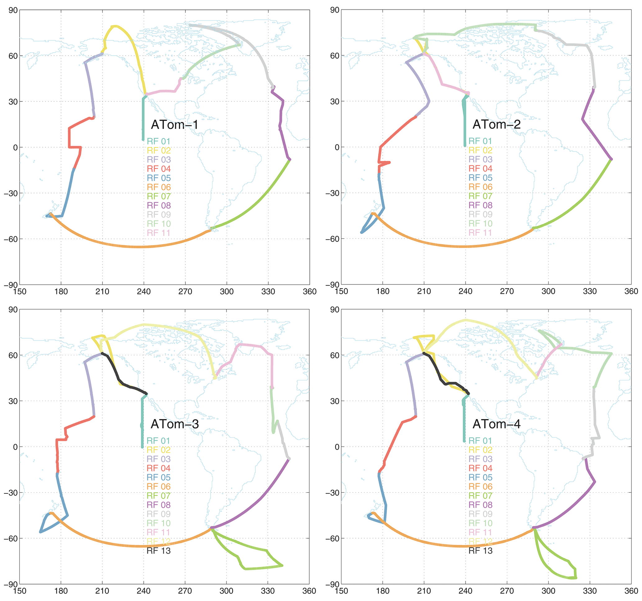
Figure 1 Map of ATom-1234 flights noting the research flight number for each deployment. The flight sequence is counterclockwise, starting at Palmdale, CA. The first research flight of each deployment is the transect from CA nearly to the Equator along 121^∘ W. The dates of each deployment are ATom-1, 29 July–23 August 2016; ATom-2, 26 January–21 February 2017; ATom-3, 28 September–27 October 2017; and ATom-4, 24 April–21 May 2018.

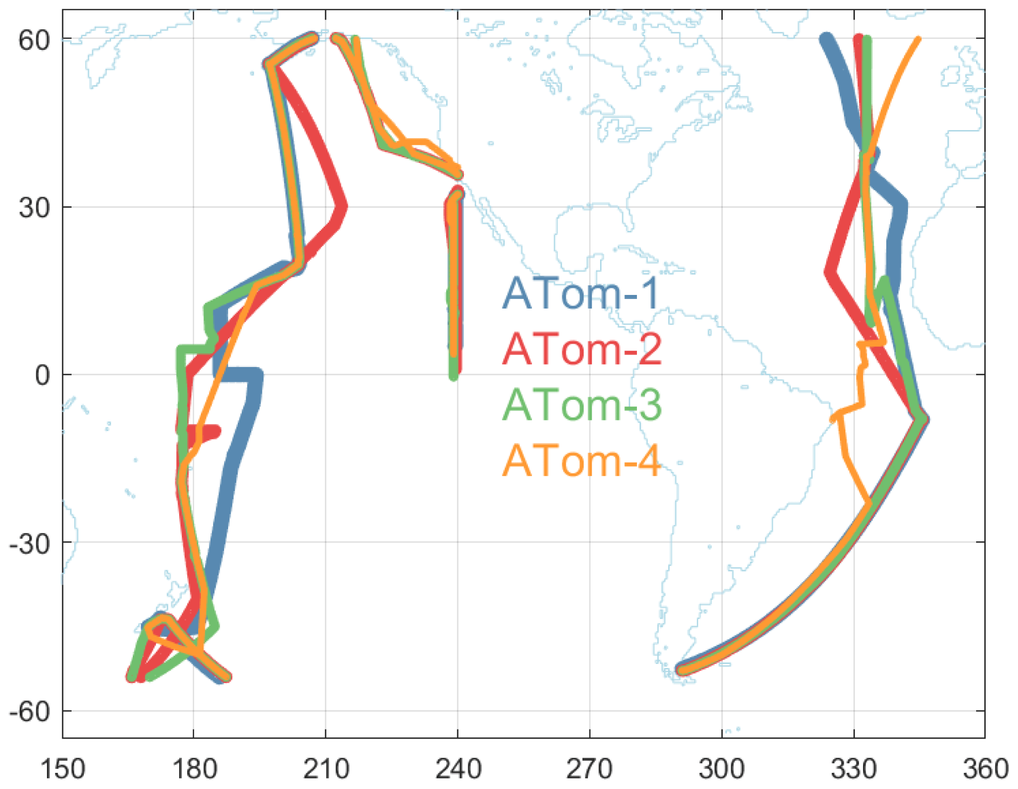
Figure 2 Map of the portion of ATom-1234 flights included in the Pacific and Atlantic basin analysis. Flight tracks are plotted in successively thinner lines to see the overlap. These flights comprise 91 912 parcels out of the total of 146 494.

2 Methods, measurements, and outline

2.1 Reactivities

Our interests in the reactivity of air parcels or model grid cells began with P2017 and continued with P2018 and G2023. We focused on the budgets of O₃ and CH₄ and now add CO. Reactivities are defined by a few key reaction rates.

Loss of CH₄ (L-CH4):

$$\begin{array}{}\text{(R1)}& {\mathrm{CH}}_{\mathrm{4}}+\mathrm{OH}\to {\mathrm{CH}}_{\mathrm{3}}+{\mathrm{H}}_{\mathrm{2}}\mathrm{O}.\end{array}$$

Production of O₃ (P-O3):

$$\begin{array}{}\text{(R2a)}& {\displaystyle }{\mathrm{HO}}_{\mathrm{2}}+\mathrm{NO}\to {\mathrm{NO}}_{\mathrm{2}}+\mathrm{OH},\text{(R2b)}& {\displaystyle }{\mathrm{RO}}_{\mathrm{2}}+\mathrm{NO}\to {\mathrm{NO}}_{\mathrm{2}}+\mathrm{RO},\text{(R2c)}& {\displaystyle }{\mathrm{O}}_{\mathrm{2}}+hv\to \mathrm{O}+\mathrm{O}\left(x\mathrm{2}\right).\end{array}$$

Loss of O₃ (L-O3):

$$\begin{array}{}\text{(R3a)}& {\displaystyle }{\mathrm{O}}_{\mathrm{3}}+\mathrm{OH}\to {\mathrm{O}}_{\mathrm{2}}+{\mathrm{HO}}_{\mathrm{2}},\text{(R3b)}& {\displaystyle }{\mathrm{O}}_{\mathrm{3}}+{\mathrm{HO}}_{\mathrm{2}}\to \mathrm{OH}+{\mathrm{O}}_{\mathrm{2}}+{\mathrm{O}}_{\mathrm{2}},\text{(R3c)}& {\displaystyle }\mathrm{O}{(}^{\mathrm{1}}\mathrm{D})+{\mathrm{H}}_{\mathrm{2}}\mathrm{O}\to \mathrm{OH}+\mathrm{OH}.\end{array}$$

Loss of CO (L-CO):

$$\begin{array}{}\text{(R4)}& \mathrm{CO}+\mathrm{OH}\to {\mathrm{CO}}_{\mathrm{2}}+\mathrm{H}.\end{array}$$

In addition, we include statistics on two key photolysis rates that drive the chemistry.

Photolysis of O₃ yielding O(¹D) (J-O1D):

$$\begin{array}{}\text{(R5)}& {\mathrm{O}}_{\mathrm{3}}+hv\to \mathrm{O}{(}^{\mathrm{1}}\mathrm{D})+{\mathrm{O}}_{\mathrm{2}}.\end{array}$$

Photolysis of NO₂ (J-NO2):

$$\begin{array}{}\text{(R6)}& {\mathrm{NO}}_{\mathrm{2}}+hv\to \mathrm{NO}+\mathrm{O}.\end{array}$$

These rates are readily diagnosed in most CCMs. We found that the net P-O3 minus L-O3 describes the 24 h O₃ tendencies over the ocean basins but not exactly as expected, and particularly not in highly polluted regions (G2023). Reaction (2c) is important in the tropospheric budget of O₃ only above ATom flight levels (12 km, Prather, 2009). In terms of the overall CO budget, we lack the chemical production of CO from CH₄ and other volatile organic compounds.

We focus on the Pacific and Atlantic oceanic flights of ATom, which we constrain to be 53^∘ S to 60^∘ N (see the map of included flights in Fig. 2), because these two ocean basins dominate the loss of CH₄ and O₃ and are a large part of the production of O₃ in most CCMs (P2017). The tropics clearly dominate the chemical budgets, and we single out the three ATom-measured regions: the central Pacific (30^∘ S–30^∘ N, about the dateline), eastern Pacific (0–30^∘ N, ∼ 121^∘ W, the first flight of each deployment to and from Palmdale), and tropical Atlantic (30^∘ S–30^∘ N). The Southern Ocean (66–55^∘ S, the Christchurch to Punta Arenas flight) and two polar regions (Arctic, > 66^∘ N; Antarctic, < 66^∘ S) are also examined separately. Only over-ocean data are analyzed here, except for the two polar regions.

2.2 Protocols

The ATom observations used for the reactivity calculations here are taken from the Modeling Data Stream (MDS-2b) described in G2023 and available at Prather et al. (2023). When completing this analysis, it was found that the method of gap-filling for NO_x did not take advantage of all the observations (i.e., flight segments where NO was measured but NO₂ was not). Thus, the updated NO_x gap-filling MDS-3 was developed.

The Reactivity Data Stream (RDS) reports the reactivities listed above plus the net 24 h change in O₃ for all 145 388 parcels, land or ocean. (Research flight number 11 of ATom-4 was a ferry flight from Greenland to Maine without profiling for which many instruments were shut down, and thus the 1106 parcels have NaN values for the MDS and RDS.) Reactivity calculations here use the UC Irvine Zhu (UCIZ) model and the RDS* protocol described in G2023. UCIZ is the updated UCI chemistry-transport model (CTM version q7.4) by Xin Zhu that is adapted to calculating ATom air parcels. The RDS^* protocol allows the peroxyacetyl nitrate (PAN) and HNO₄ species to thermally decay for 24 h before use. The overall ATom protocol for the CTM and CCMs averages 5 d, separated by 5 d centered on each deployment's central month (ATom-1, August; ATom-2, February; ATom-3, October; ATom-4, May) to average over the cloud fields (see P2017 and P2018).

The ATom RDS protocol for the CTM and CCMs is to locate the nearest model grid cell, place the ATom air parcel in that cell (along with all the other parcels in their own cells), and then integrate for 24 h (usually starting at 00:00 UTC). The problem is that many 10 s parcels may lie in the same grid cell. We use the following nested search algorithm to locate an unoccupied cell nearby: (first) search E–W from −8 to +8 longitude-shifted cells; (second) search up–down in pressure by −2 to +2 levels; and (third) search N–S from −2 to +2 latitude-shifted cells. With our 1.1^∘ CTM, we are always able to find an empty cell; however, the latitude, longitude, and pressure of the grid cell may differ from the ATom-measured value. Figure 3 shows the ATom value (MDS, x axis) vs. the CTM grid-cell value (RDS, y axis) for the 32 383 parcels of ATom-1. The mean errors in placement are very small, and even the root-mean-square error (RMSE) is modest (±1.7^∘ latitude, ±5.7^∘ longitude, ±15.3 hPa).

The CTM or CCM is run for 24 h without advection, convection, or other mixing and without wet scavenging or dry deposition or emissions. These requirements are critical because otherwise the air parcel's evolution would depend on the composition of neighboring cells, which are unknown from the ATom measurements. The key model-dependent quantities that control the reactivities are the photolysis rates, which depend on clouds and the overhead column ozone. Figure 4 compares the J values and reactivities for the ATom-1 parcels calculated for day numbers 213 (1 August) and 223 (11 August). The J values have the largest scatter, and this drives a reduced level of scatter in reactivities. The J-NO2 value is not much affected by the overhead ozone column, and so we conclude that the scatter in J values and reactivities is driven primarily by the time-varying cloud fields. (The UCI CTM uses 3 h averaged cloud fields.) The O₃ tendency (dO${}_{\mathrm{3}}/$dt) has less scatter than any of the four reactivities (P-O3, L-O3, L-CH4, L-CO) because the production and loss co-vary with clouds and their net difference has less scatter.

We expect the abundance of the reactive species to evolve over the 24 h period of the reactivity calculation, and this is documented in Fig. 5. Species with no sources because emissions are shut off decrease over the 24 h (CO, C₂H₆, alkane, alkene). NO_x systematically decreases because there are no direct emissions and HNO₃ is a major sink. HOOH systematically increases because wet scavenging is turned off. O₃ and PAN show plus–minus scatter. HNO₃ increases at values less than 2 ppb but decreases at the highest values (∼ 3 ppb). In terms of the calculation of ATom reactivities, the scatter is not worrisome, but the systematic shifts in HOOH and NO_x are a concern. The P2017 experiments showed that, averaged over an ocean basin, the reactivities with all processes running for 24 h vs. the ATom protocol were similar. A protocol that slowly removed HOOH and added NO_x is tempting but would require some arbitrary parameterizations.

2.3 Outline

Latitude-by-altitude curtain plots of the reactivities along flight tracks are presented in Sect. 3 along with reactivity statistics of the means and extremes, altitude mean profiles, and probability densities. In Sect. 4, we analyze the sensitivities of the reactivities to each of the observed species for ATom-1. These sensitivities identify those critical species where a model bias will introduce large errors into the O₃ and CH₄ budgets. In Sect. 5, we examine the impacts of MDS-3 on these analyses, and we introduce probability densities for some critical species as a possible model metric. In Sect. 6, we show how the ATom parcel reactivities and sensitivities can be used to derive chemical feedbacks, such as the lifetime for O₃ perturbations and the CH₄ lifetime feedback factor. Section 7 concludes this analysis.

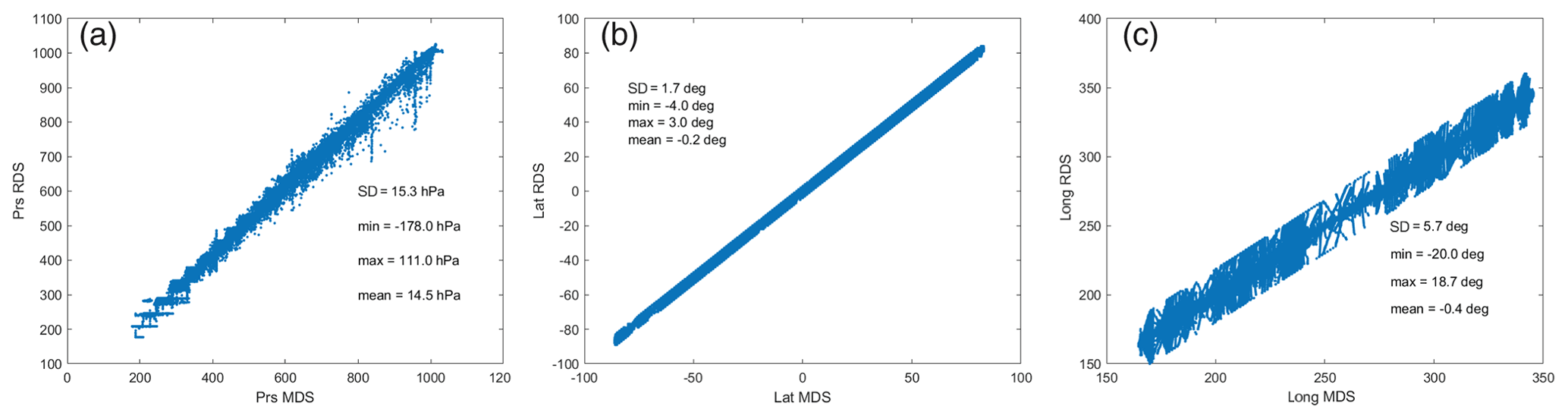
Figure 3 Comparison of the model grid-cell value for pressure, latitude, and longitude used in the RDS calculation with those from the 32 383 10 s ATom-1 parcels (MDS). In each figure the standard deviation, minimum error, maximum error, and mean error are shown. Values are specific to the UCI CTM with a T159L57 grid. These displacement errors occur because several 10 s parcels often occur within one CTM cell and must be shifted to nearby vacant cells.

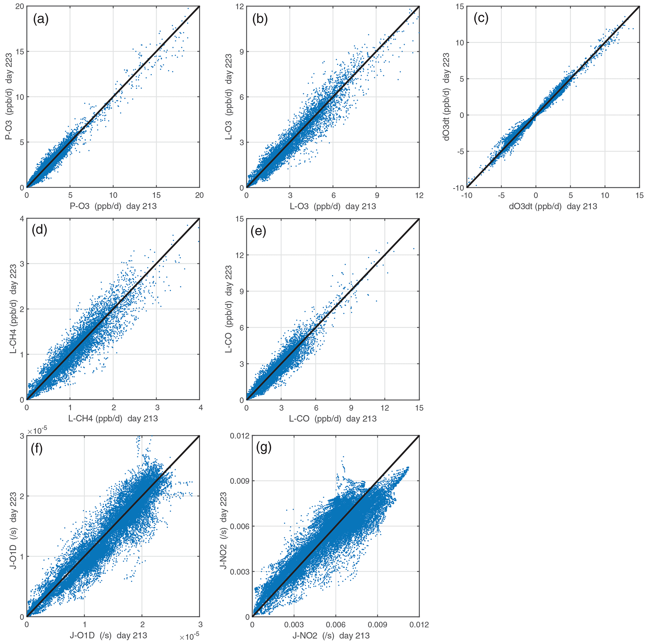
Figure 4 Reactivities (ppb d⁻¹) and J values (s⁻¹) calculated for all 32 383 ATom-1 10 s parcels using 2 different days with different cloud fields and ozone columns. The net integrated ozone change over the day, dO${}_{\mathrm{3}}/$dt (ppb d⁻¹), is also shown. Day 213 is 1 August, and day 223 is 11 August. Mean reactivity statistics here are calculated as the mean of five days (1, 6, 11, 16, and 21 August), while sensitivity analyses used only day 223.

Figure 5 The input–output values of reactive species showing the 24 h change from the ATom-1 MDS input value (x axis) to the final value (y axis) calculated following the ATom protocol in the UCI CTM. First row: O₃, NO_x, PAN. Second row: HONO₂, CO, C₂H₆. Third row: alkane (C₃₊), alkene (C₂H₄), H₂O₂. Fourth row: CH₃OOH (MeOOH), CH₃CHO (MeCHO), HCHO.

3 Variation of photochemical reactivities across the four ATom deployments

3.1 Reactivity statistics – means and extremes

We developed statistics that identify extremes (i.e., photochemical hotspots) and characterize the heterogeneous mixture of air parcels. Table 1 presents the means and medians of each of the four reactivities (P-O3, L-O3, L-CH4, L-CO) and two J values (J-O1D, J-NO2) for each of the eight regions (Pacific, Atlantic, central tropical Pacific, eastern tropical Pacific, tropical Atlantic, Southern Ocean, Arctic, Antarctic) and four deployments (ATom-1234 in August, February, October, and May, respectively). Each 10 s parcel is weighted to give equal sampling by mass from 0 to 12 km for each 10^∘ latitude bin or a single latitude bin for polar latitudes. The extreme statistics look at the top 50 %, 10 %, and 3 % of the weighted parcels, giving the mean reactivity in those ranges and the fraction of the total weighted reactivity in those upper ranges.

Table 1 Statistics on reactivities R and J values by basin and deployment.

The primary ocean basins (Pacific and Atlantic) use the over-ocean flight data from 53^∘ S to 60^∘ N (see Fig. 2). The tropical ocean sections are the central Pacific (30^∘ S–30^∘ N, near the dateline), eastern Pacific (0–30^∘ N, ∼ 121^∘ W), and tropical Atlantic (30^∘ S–30^∘ N). All 10 s data are weighted inversely by frequency of occurrence at 10^∘ latitude by 100 hPa bins and by cosine (latitude). For the high-latitude sections – Arctic (66^∘ N–90^∘ N), Southern Ocean (66–55^∘ S), and Antarctica (90–66^∘ S) – parcels are weighted only by frequency of occurrence in 100 hPa bins.

Starting with the Pacific and Atlantic basins, we see that the average photolysis rates (J-O1D, J-NO2, Table 1) have little seasonality (variation across deployments) and further have a flat distribution with the median greater than the mean. For P-O3 (Table 1) the Atlantic mean is slightly larger (10 %–20 %) than the Pacific mean except for ATom-2. The medians are always smaller than the mean. The reactivity of the top 10 % is about 2.5 times that of the mean, indicating that a distribution peaked in photochemical hotspots. For L-O3 (Table 1) the Atlantic mean is much larger (30 %–50 %) than the Pacific mean, and the extreme statistics are similar. What is unusual is that ATom-1 has the lowest mean P-O3 in both the Pacific and Atlantic, while it has a high L-O3 or the highest L-O3. Thus, ATom-1 has a distinctly different mixture of species than ATom-234. A clear seasonality is seen for L-O3, with ATom-2 (February) having the lowest reactivities, presumably due to the reduced activity of northern mid-latitude continental pollution in winter. L-CO (Table 1) shows similar patterns to L-O3 (lowest in ATom-2 Pacific, highest in ATom-1 Atlantic), while that of L-CH4 (Table 1) is more uniform across deployments. This feature can be seen in the curtain and mean profile plots, where L-CH4 is restricted to the lower troposphere due to the high temperature sensitivity of the rate coefficient for Reaction (R1).

The Arctic region is highly seasonal, and photochemistry mostly shuts down in ATom-2 and ATom-3 (February and October), but it is quite reactive in ATom-1 and ATom-4 (August and May). This is seen clearly in the J values (Table 1), particularly J-O1D, which is the primary source of OH. The Arctic reactivities in ATom-1 and ATom-4 are about two-thirds of the mean Pacific and Atlantic values year round, with the exception of L-CH4, which is extremely repressed due to the colder Arctic temperatures in all seasons. The extreme statistics in the Arctic are similar to the Pacific and Atlantic except for P-O3 in ATom-234, which is dominated by hot parcels. Note that we have excluded the stratospheric parcels in these statistics (see the Supplement of G2023).

The Southern Ocean has high reactivities for ATom-2 and ATom-3 as expected for austral summer. L-O3 and L-CO are about half the reactivity of the Arctic for the complementary seasons, but P-O3 and L-CH4 are more similar to the Arctic. Clearly, the chemical mixture of these two regions is different. The extreme statistics for the Southern Ocean are similar to the Arctic.

The Antarctic flights of ATom were a target of opportunity for ATom-3 and ATom-4. ATom-4 (May) was too dark to have significant reactivity (extremely low J values, Table 1). ATom-3 Antarctica has distinctly lower reactivities than ATom-3 Southern Ocean except for P-O3, which is surprisingly comparable.

Figure 6 Two-dimensional curtain plots (altitude–latitude profiling) of P-O3 (ppb d⁻¹) in the Pacific basin (53^∘ S–60^∘ N) for ATom-1234. In all these curtain plots, ATom 10 s parcel data are weighted by cosine (latitude) and sampling frequency, and then they are averaged into 1^∘ latitude and 200 m altitude bins.

Figure 7 Curtain plots of L-O3 (ppb d⁻¹) in the Pacific basin (53^∘ S–60^∘ N) for ATom-1234. See Fig. 6.

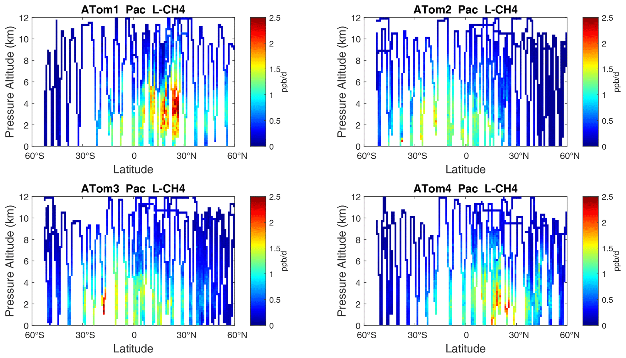
Figure 8 Curtain plots of L-CH4 (ppb d⁻¹) in the Pacific basin (53^∘ S–60^∘ N) for ATom-1234. See Fig. 6.

3.2 Curtain plots

The spatial structures and variability of P-O3 as sampled by the four ATom transects over the Pacific Ocean are presented as 2D latitude–height curtain plots in Fig. 6. The full sets of plots covering all four reactivities and also the Atlantic Ocean are shown sequentially in Figs. 6–13. For these curtain plots, the 10 s reactivities (2 km-by-80 m thick parcels) are averaged and plotted at 1^∘ latitude by 200 m thick cells. For both the Atlantic and Pacific basins, the reactivities (L-O3, L-CH4, and L-CO) generally follow the Sun, with more southerly hot parcels in ATom-23 (February, October) and northerly hot parcels in ATom-14 (August, May). The P-O3 hotspots have no simple seasonality, being dominated by middle- to upper-tropospheric regions with high NO_x presumably from the outflow of deep convection from the nearby continents.

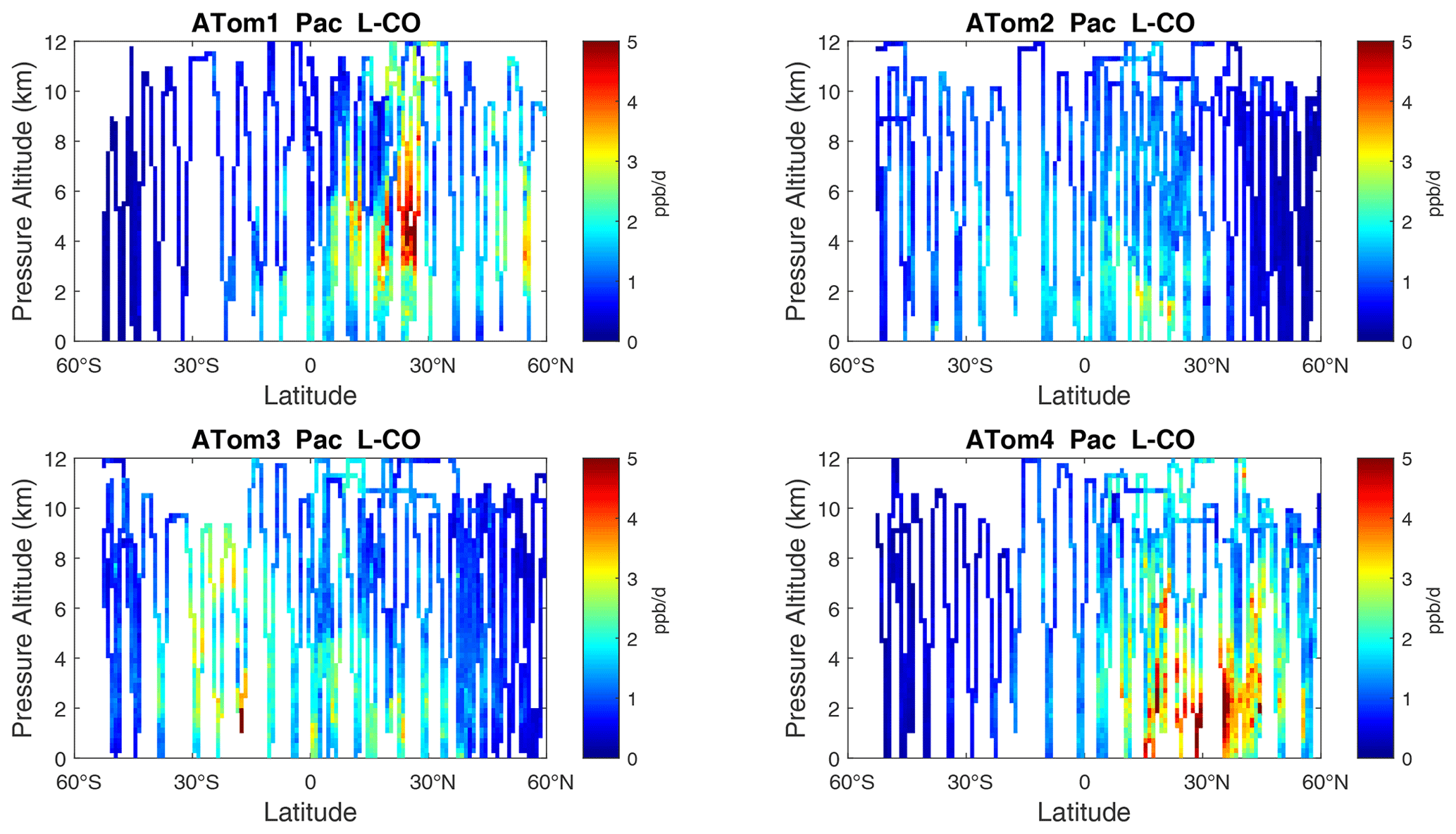
Figure 9 Curtain plots of L-CO (ppb d⁻¹) in the Pacific basin (53^∘ S–60^∘ N) for ATom-1234. See Fig. 6.

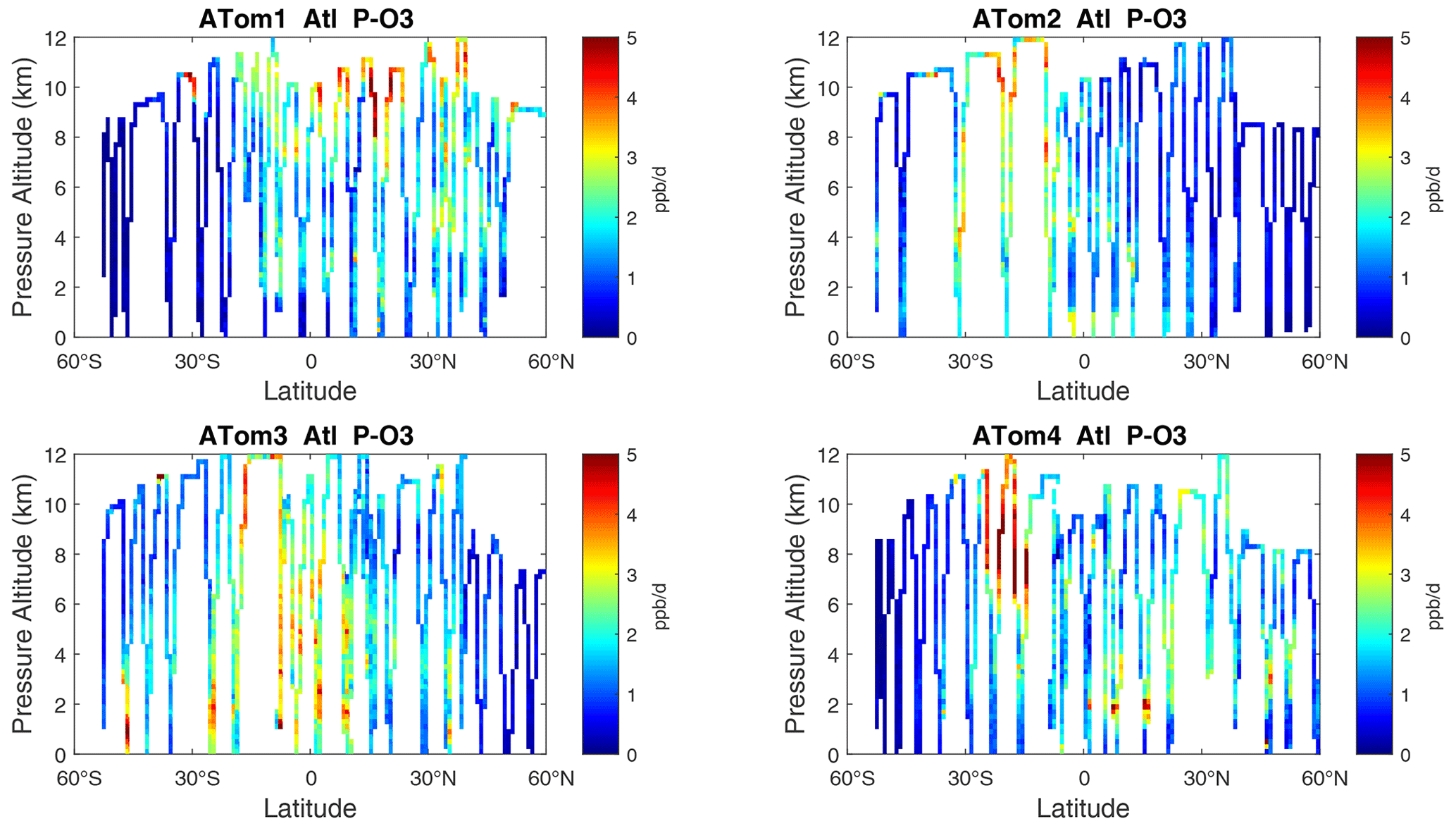
Figure 10 Curtain plots of P-O3 (ppb d⁻¹) in the Atlantic basin (53^∘ S–60^∘ N) for ATom-1234. See Fig. 6.

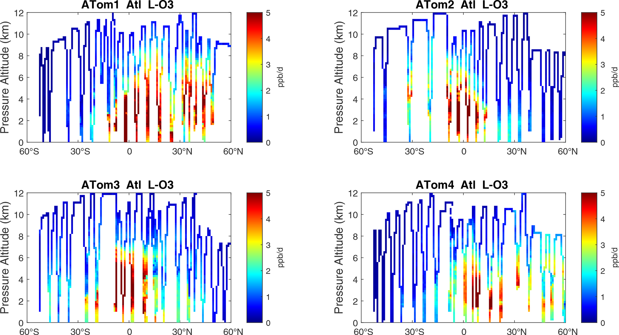
Figure 11 Curtain plots of L-O3 (ppb d⁻¹) in the Atlantic basin (53^∘ S–60^∘ N) for ATom-1234. See Fig. 6.

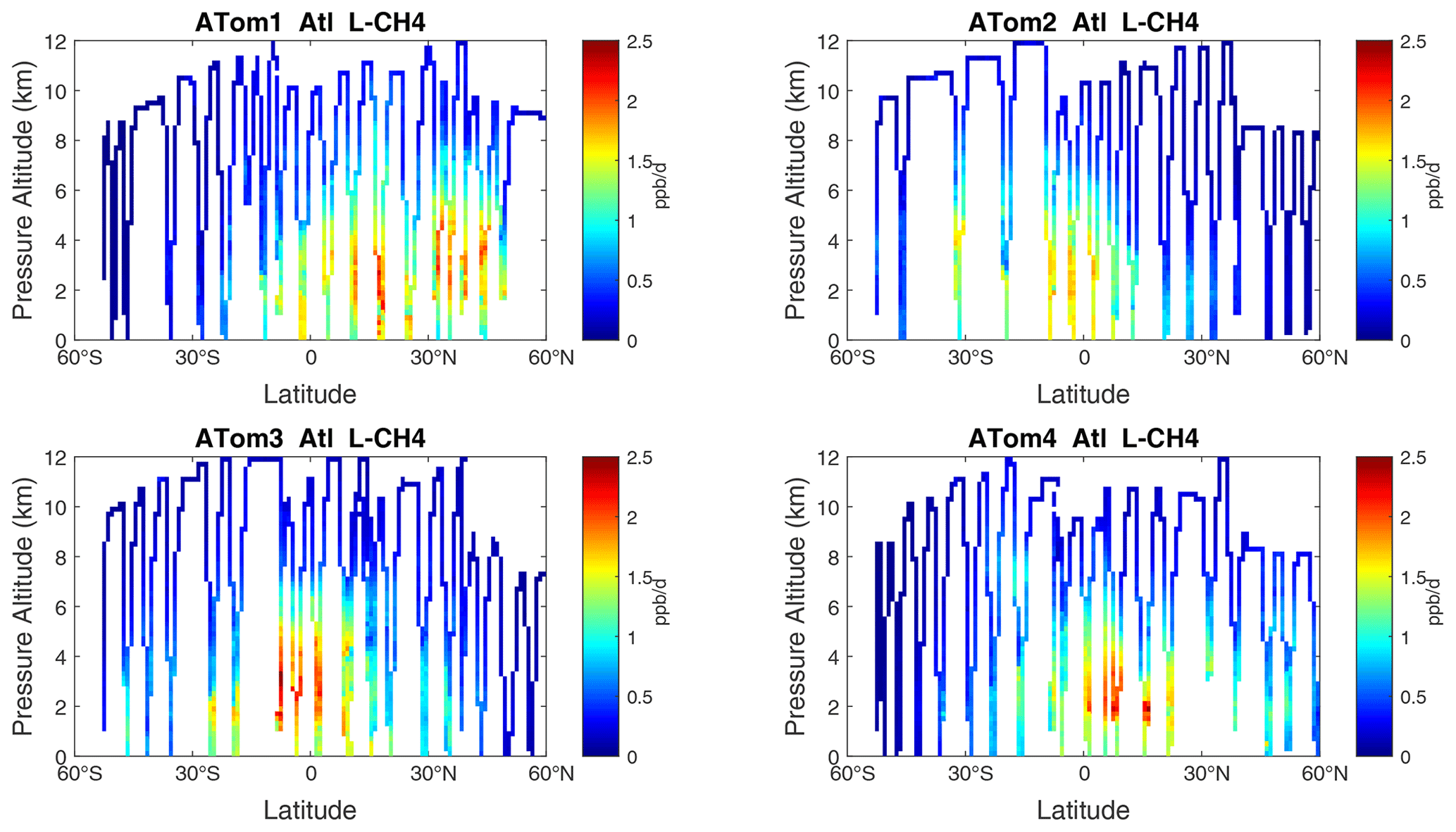
Figure 12 Curtain plots of L-CH4 (ppb d⁻¹) in the Atlantic basin (53^∘ S–60^∘ N) for ATom-1234. See Fig. 6.

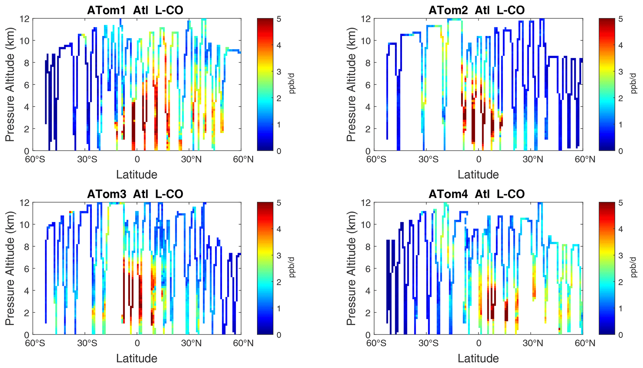
Figure 13 Curtain plots of L-CO (ppb d⁻¹) in the Atlantic basin (53^∘ S–60^∘ N) for ATom-1234. See Fig. 6.

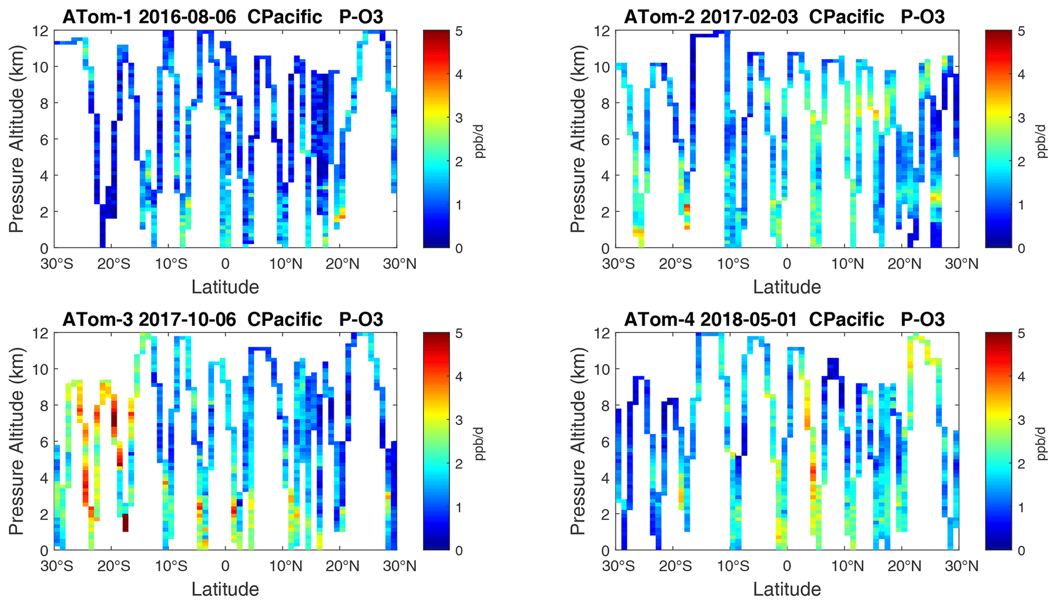
Figure 14 Curtain plots of P-O3 (ppb d⁻¹) in the tropical central Pacific (30^∘ S–30^∘ N) for ATom-1234. See Fig. 6. The dates of the flight crossing the equatorial Pacific for each deployment are given.

Because the eastern Pacific flights (∼ 121^∘ W) are clearly influenced by continental outflow from North and Central America, we separate them from the central Pacific in our examination of the tropical oceans (see Fig. 2). Curtain plots of the four reactivities for ATom-1234 in the central Pacific are shown in Figs. 14–17, in the eastern Pacific in Figs. 18–21, and in the tropical Atlantic in Figs. 22–25. In terms of P-O3, the central Pacific shows a few hotspots but generally no large regions > 3 ppb d⁻¹. The tropical Atlantic shows extensive regions in the middle to upper troposphere with P-O3 > 3 ppb d⁻¹, and these look like continental outflow with both NO_x and HO_x sources. The eastern Pacific shows extensive 1–2 km thick, 10^∘ latitude layers of mostly above 8 km. In the eastern Pacific these P-O3 layers are clearly separated from the moderately high (ATom-23) to extremely high (ATom-14) L-O3 > 5 ppb d⁻¹ layers below 8 km. The large L-O3 (and also L-CH4 and L-CO) layers contain highly reactive HO_x–VOC chemistry but little NO_x, and these are associated with continental outflow (see the discussion in G2023). The tropical Atlantic, in contrast to the central Pacific, shows large 20–30^∘ wide tropical regions below 8 km with L-O3 > 4 ppb d⁻¹, L-CH4 > 1.5 ppb d⁻¹, and L-CO > 4 ppb d⁻¹. These regions follow the sun, northward in ATom-14 and southward in ATom-23. For L-O3 and L-CO, the tropical Atlantic has 50 % greater loss than the central Pacific.

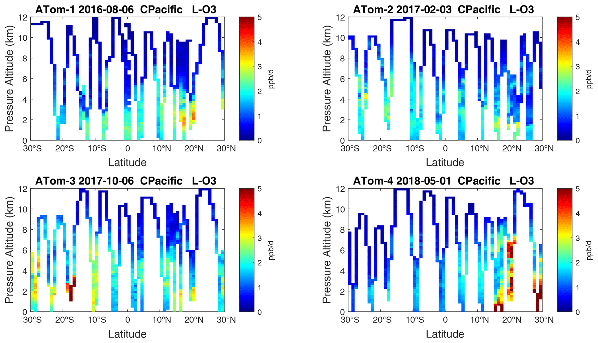
Figure 15 Curtain plots of L-O3 (ppb d⁻¹) in the tropical central Pacific (30^∘ S–30^∘ N) for ATom-1234. See Fig. 6.

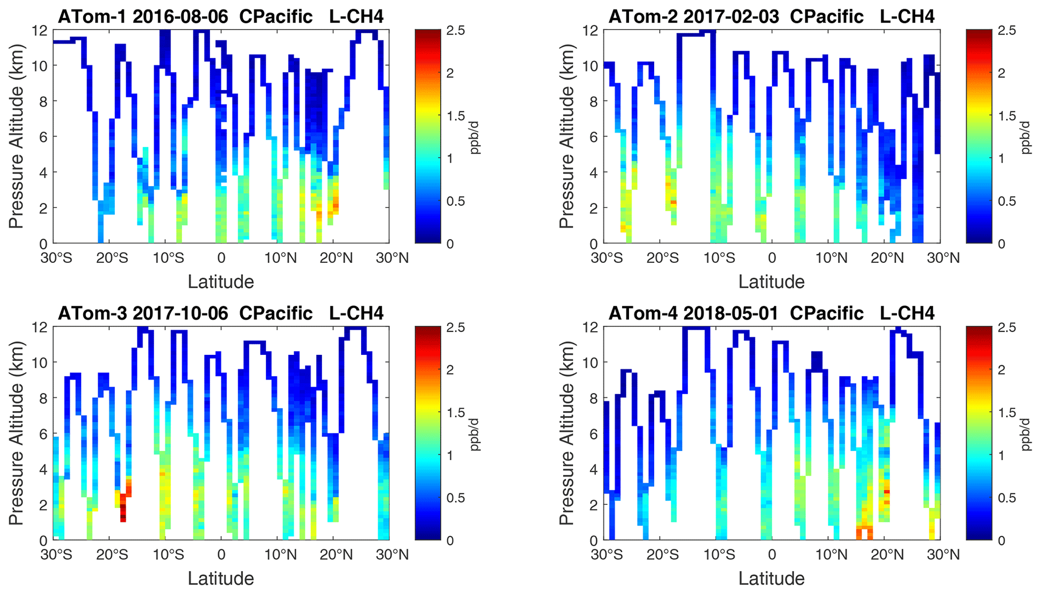
Figure 16 Curtain plots of L-CH4 (ppb d⁻¹) in the tropical central Pacific (30^∘ S–30^∘ N) for ATom-1234. See Fig. 6.

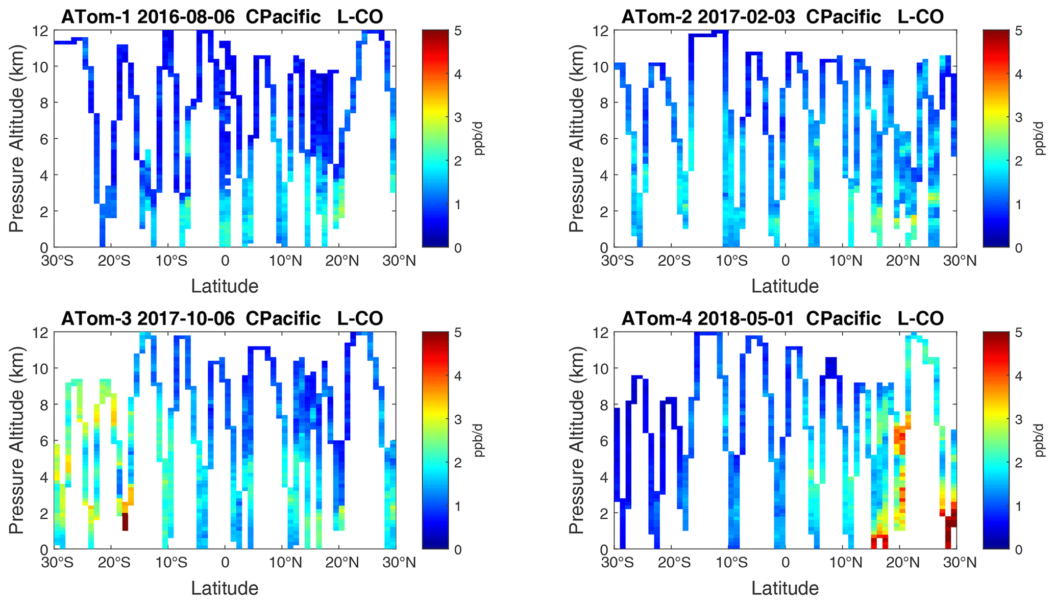
Figure 17 Curtain plots of L-CO (ppb d⁻¹) in the tropical central Pacific (30^∘ S–30^∘ N) for ATom-1234. See Fig. 6.

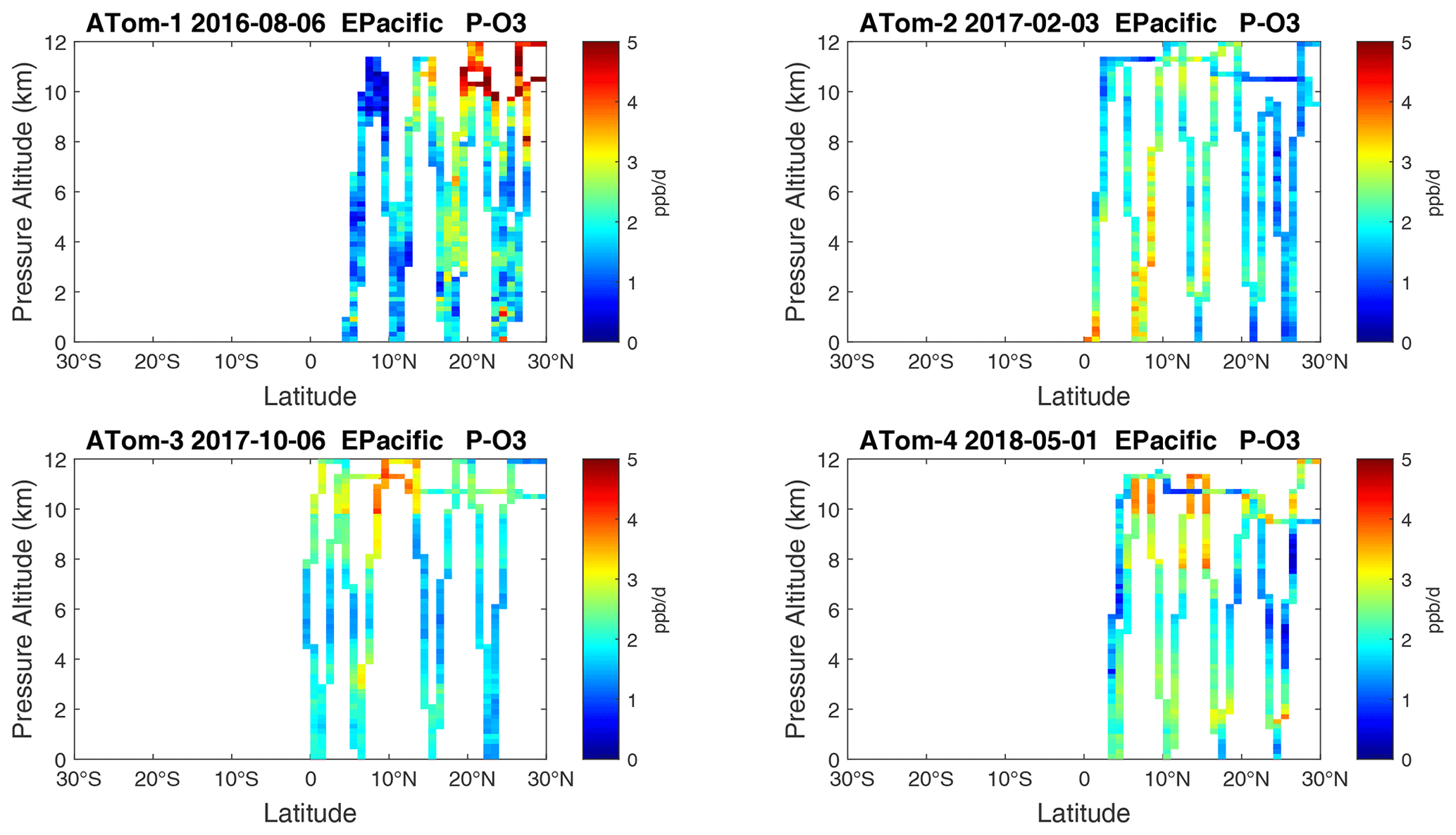
Figure 18 Curtain plots of P-O3 (ppb d⁻¹) in the tropical eastern Pacific (0–30^∘ N) for ATom-1234. See Fig. 6.

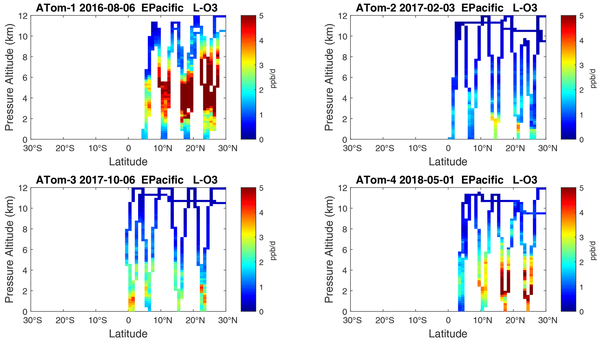
Figure 19 Curtain plots of L-O3 (ppb d⁻¹) in the tropical eastern Pacific (0–30^∘ N) for ATom-1234. See Fig. 6.

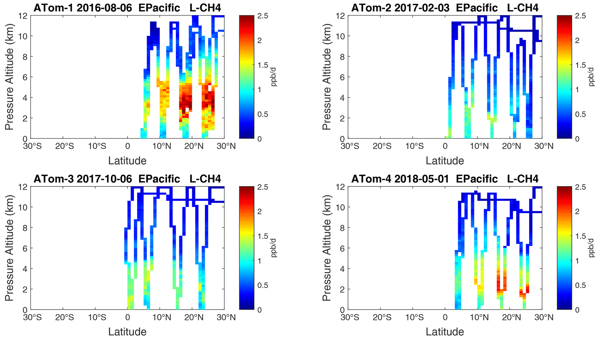
Figure 20 Curtain plots of L-CH4 (ppb d⁻¹) in the tropical eastern Pacific (0–30^∘ N) for ATom-1234. See Fig. 6.

Overall, these figures (Figs. 6–25) show the dominance of the tropics (30^∘ S–30^∘ N) for photochemical reactivity over the oceans. Only the northern mid-latitudes (30–60^∘ N) almost contribute a fifth tropic-like reactive region in summer (ATom-14), especially in the Atlantic.

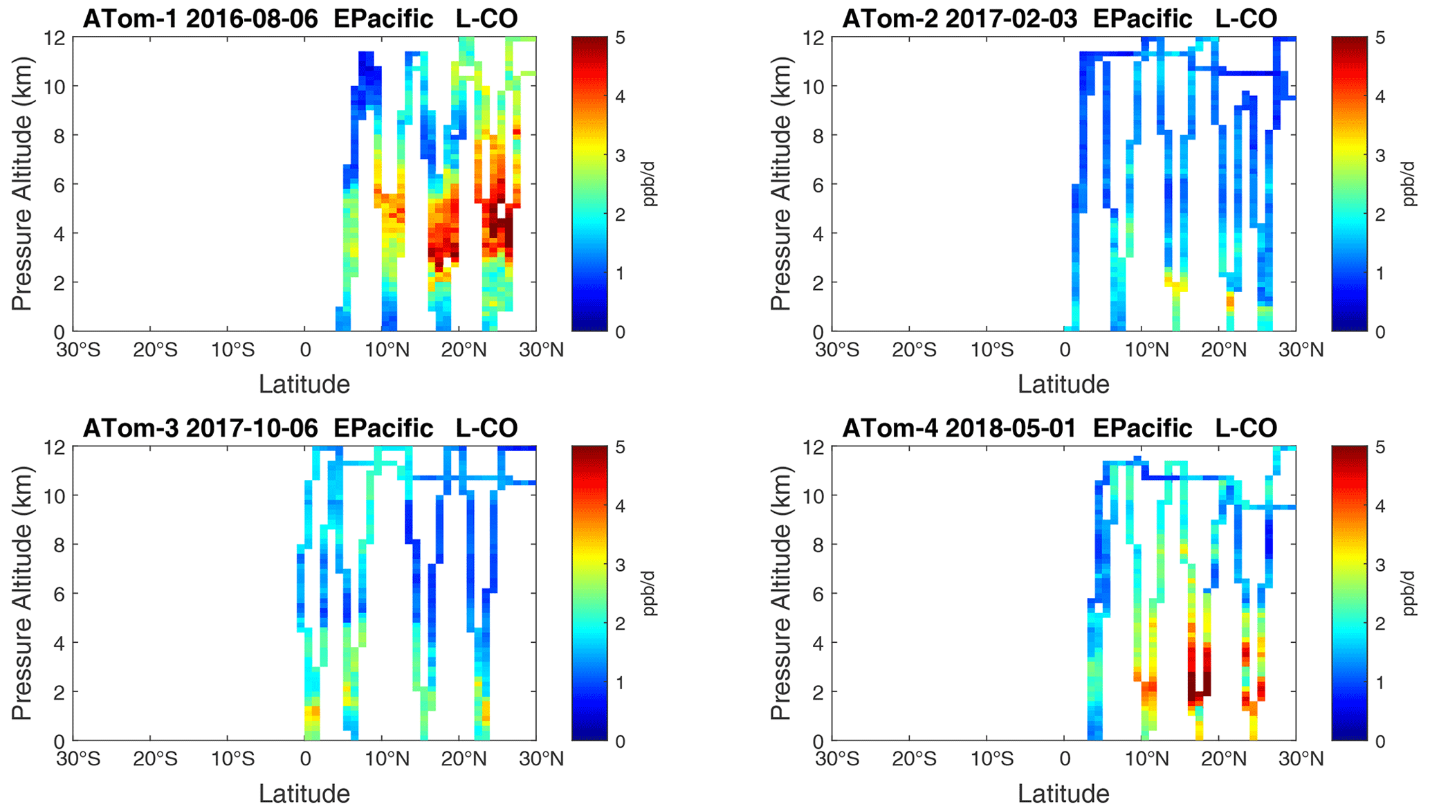
Figure 21 Curtain plots of L-CO (ppb d⁻¹) in the tropical eastern Pacific (0–30^∘ N) for ATom-1234. See Fig. 6.

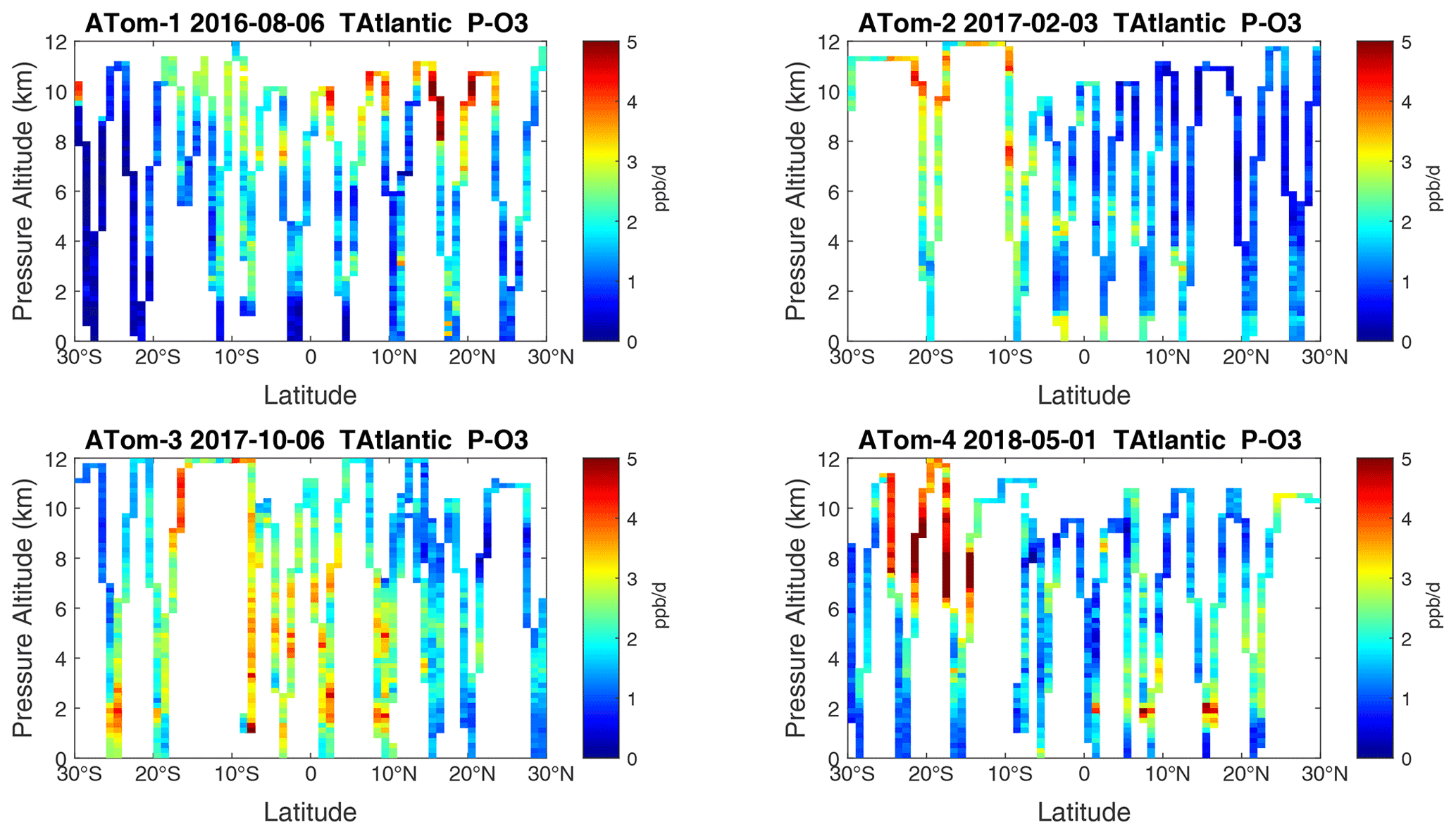
Figure 22 Curtain plots of P-O3 (ppb d⁻¹) in the tropical Atlantic (30^∘ S–30^∘ N) for ATom-1234. See Fig. 6.

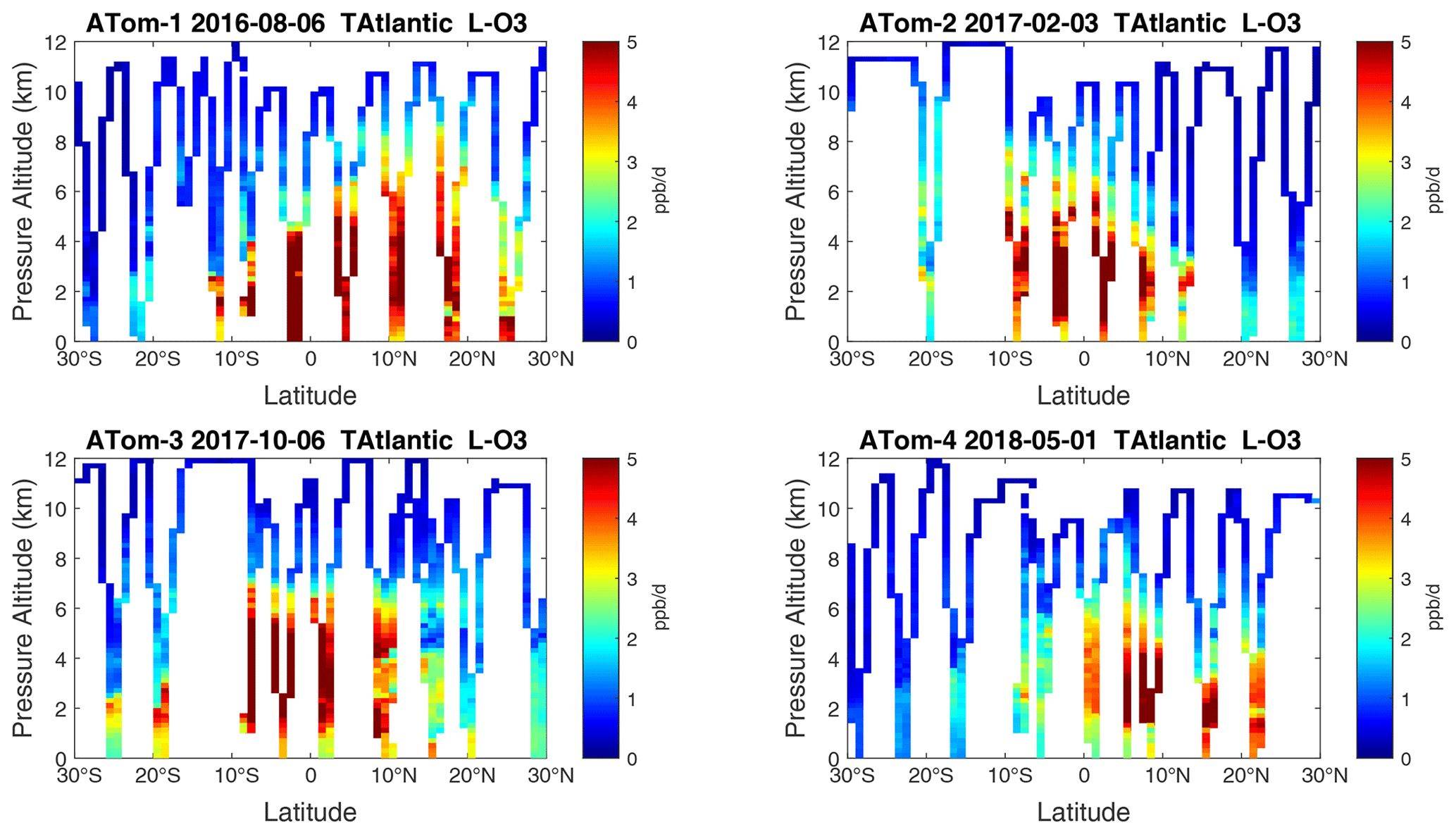
Figure 23 Curtain plots of L-O3 (ppb d⁻¹) in the tropical Atlantic (30^∘ S–30^∘ N) for ATom-1234. See Fig. 6.

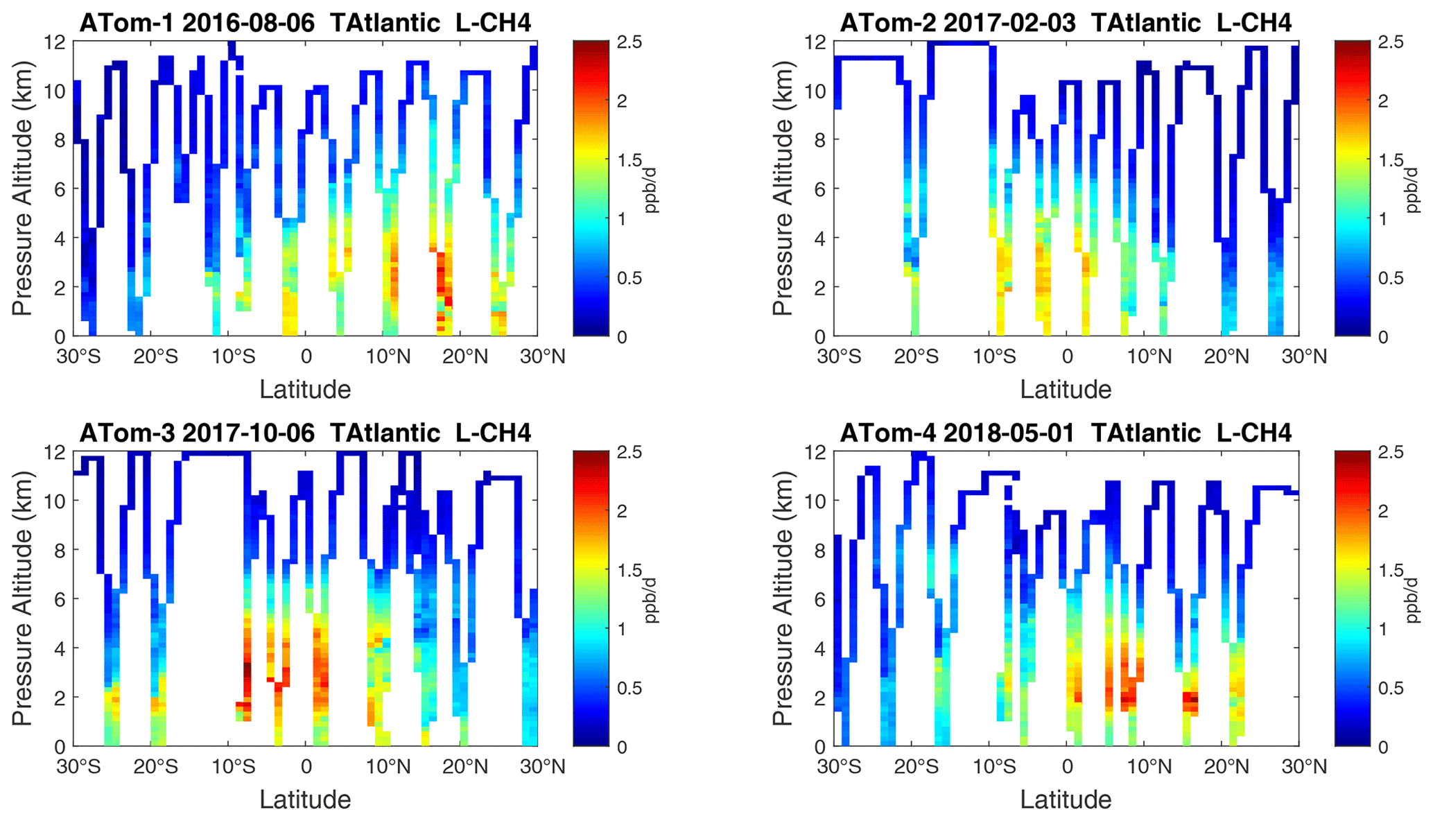
Figure 24 Curtain plots of L-CH4 (ppb d⁻¹) in the tropical Atlantic (30^∘ S–30^∘ N) for ATom-1234. See Fig. 6.

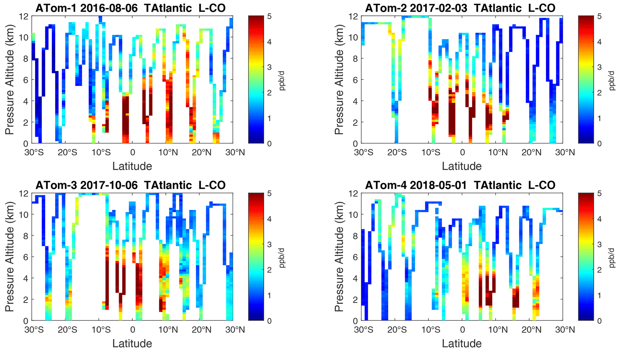
Figure 25 Curtain plots of L-CO (ppb d⁻¹) in the tropical Atlantic (30^∘ S–30^∘ N) for ATom-1234. See Fig. 6.

Curtain profiles for the Arctic are presented only for ATom-1 (Fig. 26) and ATom-4 (Fig. 27) when there was enough sunlight to generate non-negligible reactivities. The very low-reactivity statistics for ATom-23 Arctic are seen in Table 1. Stratospheric air parcels are excluded in these Arctic statistics. Reactivities appear to be moderately high, but the color scale is 3 times smaller than in Figs. 6–25. Similarly to the ocean basins, in the Arctic much of the P-O3 occurs above 8 km, and losses (L-O3, L-CH4, L-CO) occur between 1 and 6 km. Curiously, there is a region of high L-CO above 10 km in the region of high P-O3. Notably, that rate (R4) is not sensitive to cold temperatures. Only one of the two Antarctic flights had enough sunlight to produce much reactivity (ATom-3, Fig. 28). Like the Arctic, P-O3 is concentrated in the upper troposphere, while L-O3 and L-CH4 are in the lower troposphere. Note that the color scale is 6 to 12 times smaller than in Figs. 6–25.

3.3 Mean altitude profiles

Given the inherent synoptic variability plus the large seasonal shifts in chemical reactivity across the Pacific and Atlantic basins seen in the individual profiles (Figs. 6–13), one might ask how useful or representative the four ATom transects are for testing model statistics. Because the 53^∘ S–60^∘ N Pacific and Atlantic transects contain the north–south seasonal shifts and most of the reactivity (see the Southern Ocean, Arctic, and Antarctic reactivities above), a mean profile should average over some of the synoptic variability and give us a seasonal variation in the basin-mean reactivity that could test chemistry-climate models. Seasonal variability in the mean reactivity profiles is clearly due to shifts in the chemical composition caused, for example, in the Atlantic by the cycle of African biomass burning and convection. A similar reasoning applies to basin-wide probability densities (see Sect. 3.4 below).

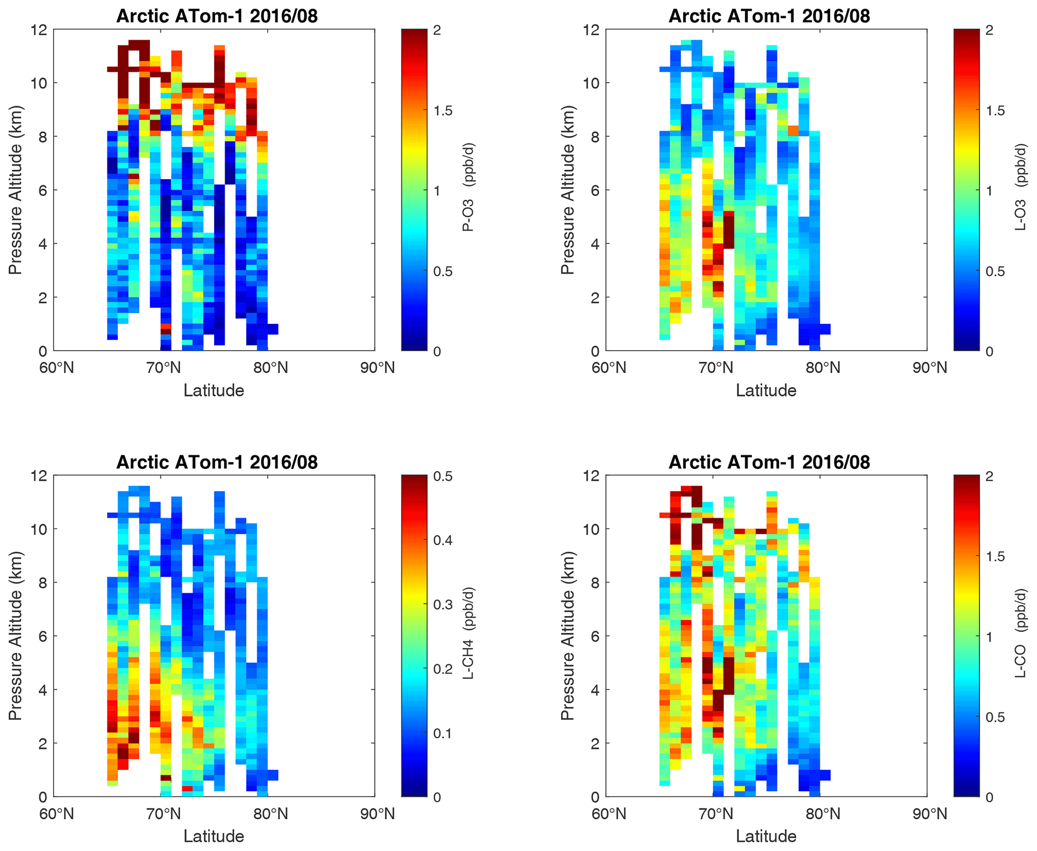
Figure 26 Curtain plots of the four reactivities (P-O3, L-O3, L-CH4, L-CO ppb d⁻¹) over the Arctic for ATom-1. Note that the color bars have a much smaller range than in the Pacific and Atlantic basin plots. Troposphere-only parcels are shown, with the stratosphere defined as H₂O < 30 ppm, O₃ > 80 ppb, and CO < 120 ppb. See Fig. 6.

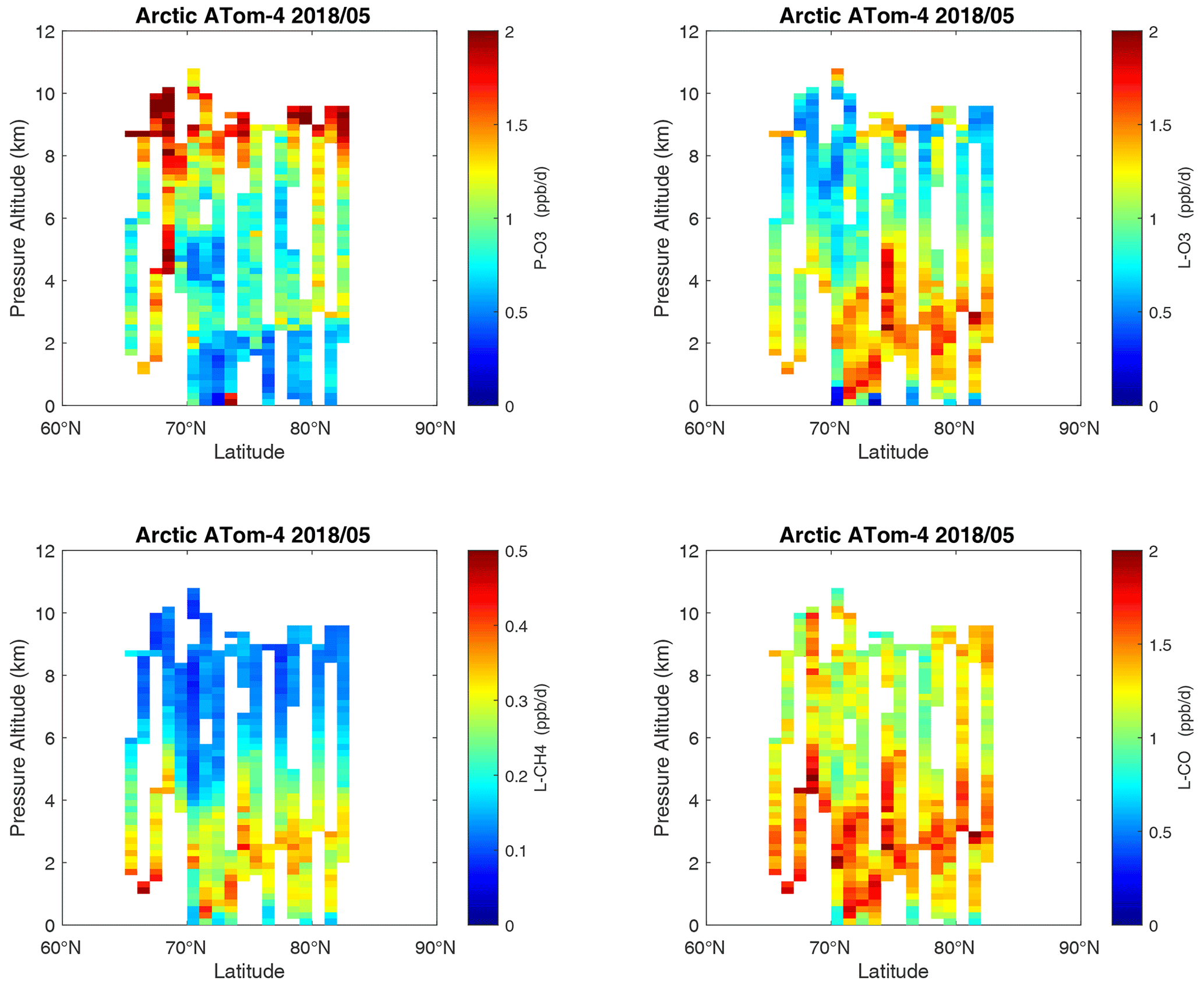
Figure 27 Curtain plots of the four reactivities (P-O3, L-O3, L-CH4, L-CO ppb d⁻¹) over the Arctic on ATom-4. Troposphere-only parcels. See Figs. 6 and 26.

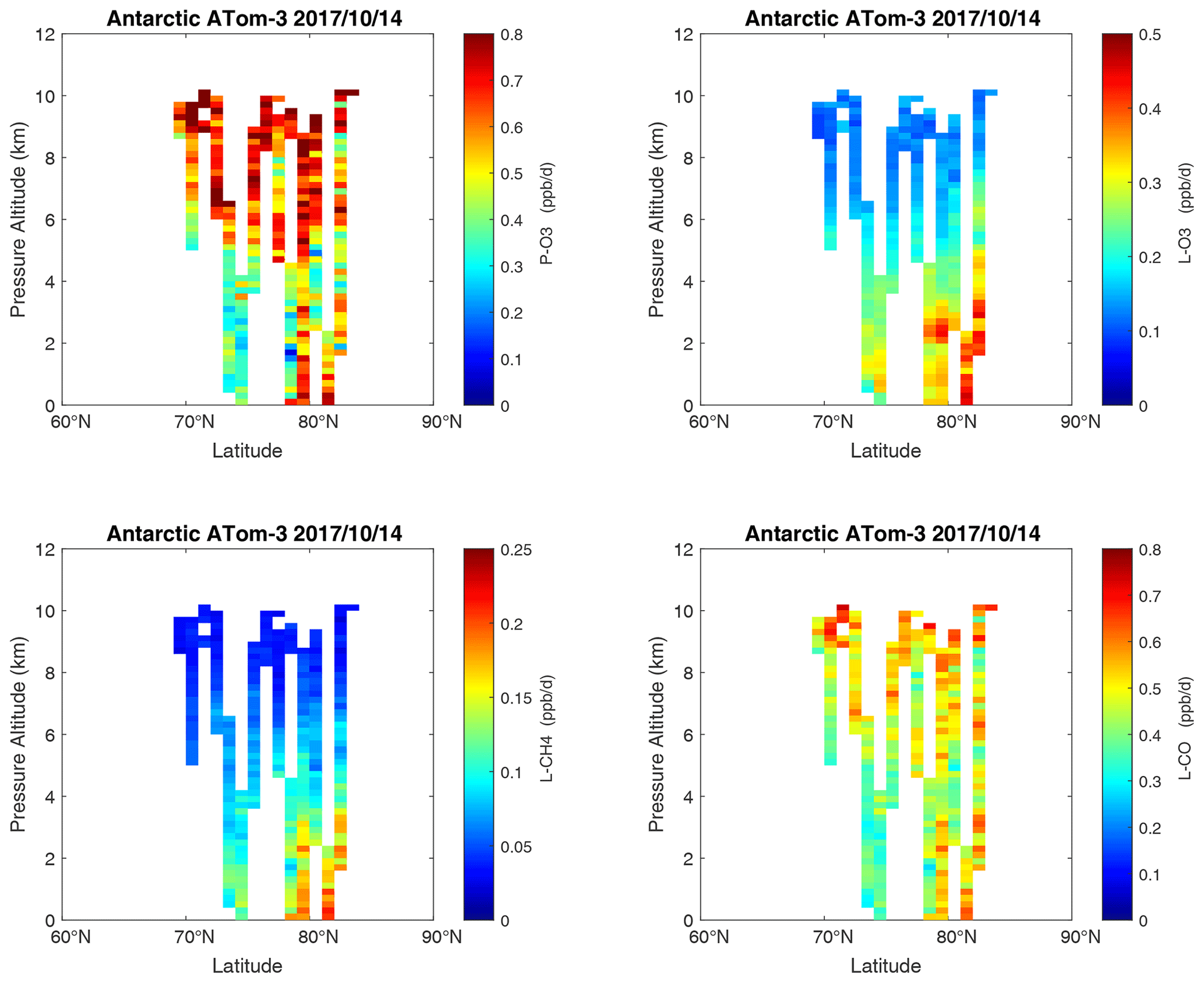
Figure 28 Curtain plots of the four reactivities (P-O3, L-O3, L-CH4, L-CO, ppb d⁻¹) over Antarctica on ATom-3. Note that the color bars have a smaller range than in the Pacific, Atlantic, and Arctic basin plots. Troposphere-only parcels. See Figs. 6 and 26.

Altitude profiles of the weighted mean P-O3 for the three tropical basins and four deployments are compared in Fig. 29. For other reactivities, see Figs. 30–32. These profiles highlight the consistency in basin averages across the four ATom deployments, with some exceptions. In the Pacific, the P-O3 profiles are similar, but ATom-1 is systematically less below 6 km. Although the hotspots of P-O3 are dominated by the higher altitudes, the mean profile shows only a modest increase above 10 km. In the Atlantic, ATom-3 has a much greater P-O3 below 6 km, but above 8 km, all the deployments show a wide range of mean values, with ATom-1 exceeding 2.5 ppb d⁻¹ above 10 km. For L-O3 and L-CH4, the spread is much larger, with ATom-1 largest in both the Pacific and Atlantic. For L-CO, the variation is different still, with a relatively large spread: e.g., in the Pacific, ATom-4 is 50 %–100 % larger than ATom-2.

Mean reactivity profiles for the three tropical basins are shown in Figs. 33–36. Here the central Pacific shows low variability across the deployments (except for the P-O3 minimum in ATom-1), while the eastern Pacific shows little range in P-O3 but very large L-O3, L-CH4, and L-CO below 8 km for ATom-14. The end of the biomass burning season in Central America (15–20^∘ N) is probably the cause of the peak L-O3 below 6 km in ATom-4 (May), while the start of the North American monsoon season is probably the cause of the extensive highly reactive deep-convection layer (2–10 km) in ATom-1 (August). With this high level of variability, it will be important to re-examine the time period of the ATom flights with a chemistry-transport model to assess the spatiotemporal scales and origins of these events.

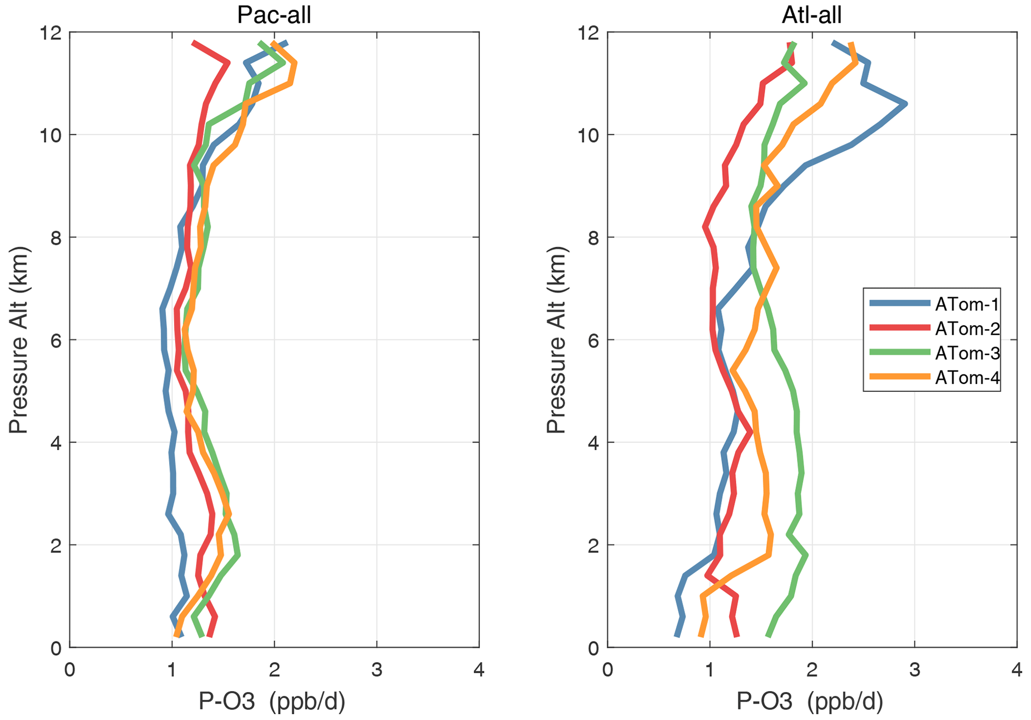
Figure 29 Mean altitude profile of P-O3 (ppb d⁻¹) over the Pacific and Atlantic basins (53^∘ S–60^∘ N) for ATom-1234.

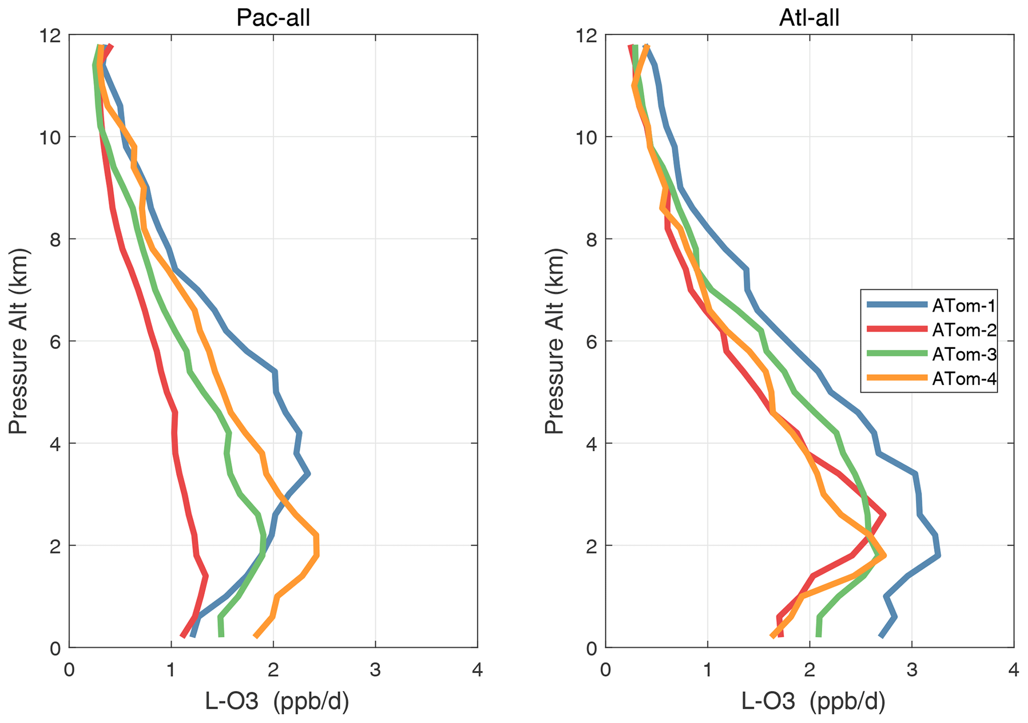
Figure 30 Mean altitude profile of L-O3 (ppb d⁻¹) over the Pacific and Atlantic basins (53^∘ S–60^∘ N) for ATom-1234.

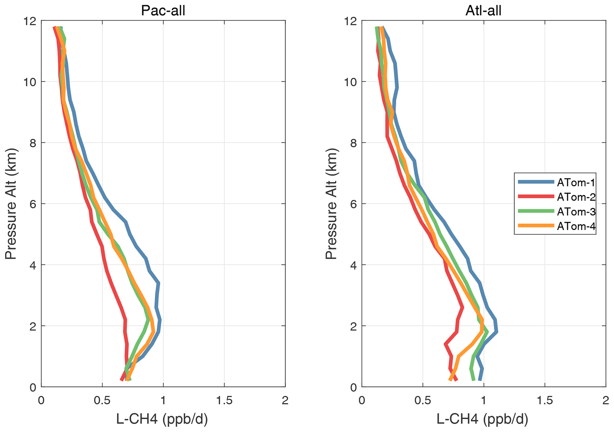
Figure 31 Mean altitude profile of L-CH4 (ppb d⁻¹) over the Pacific and Atlantic basins (53^∘ S–60^∘ N) for ATom-1234.

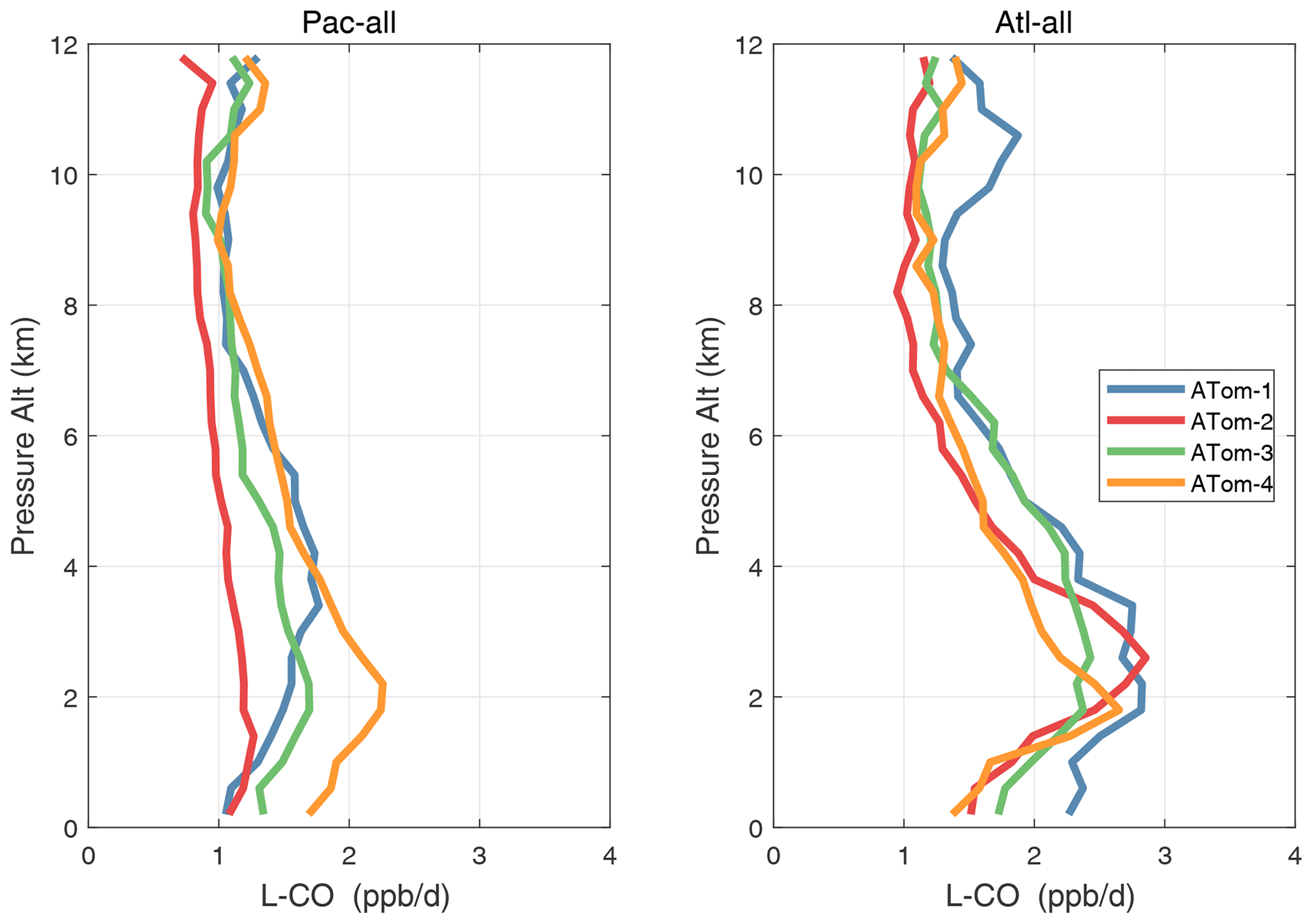
Figure 32 Mean altitude profile of L-CO (ppb d⁻¹) over the Pacific and Atlantic basins (53^∘ S–60^∘ N) for ATom-1234.

In the Arctic (Fig. 37), ATom-14 shows similar profiles but with different shapes for each reactivity, while ATom-23 has negligible reactivities, as expected from the limited sunlight. P-O3 peaks at 8–12 km with values from 1–2 ppb d⁻¹, while L-O3 and L-CH4 peak around 2–4 km. As in the curtain plots, L-CO peaks with L-O3 in the lower troposphere and also with P-O3 in the upper troposphere. The reactivities in the Arctic, even in summer, are less than the average over the Pacific and Atlantic oceans and thus have little impact on the global O₃ or CH₄ budgets.

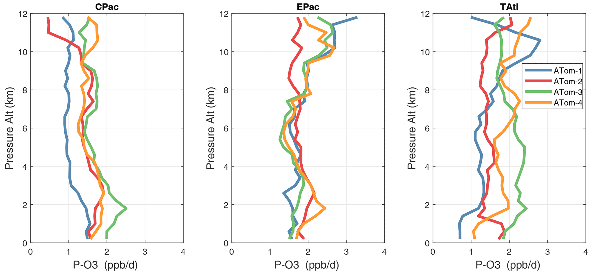
Figure 33 Mean altitude profile of P-O3 (ppb d⁻¹) over the three tropical basins for ATom-1234.

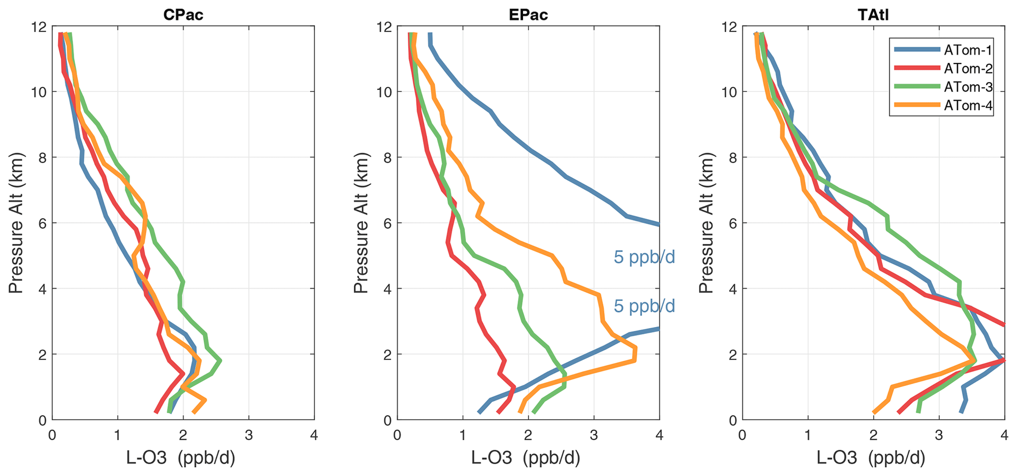
Figure 34 Mean altitude profile of L-O3 (ppb d⁻¹) over the three tropical basins for ATom-1234.

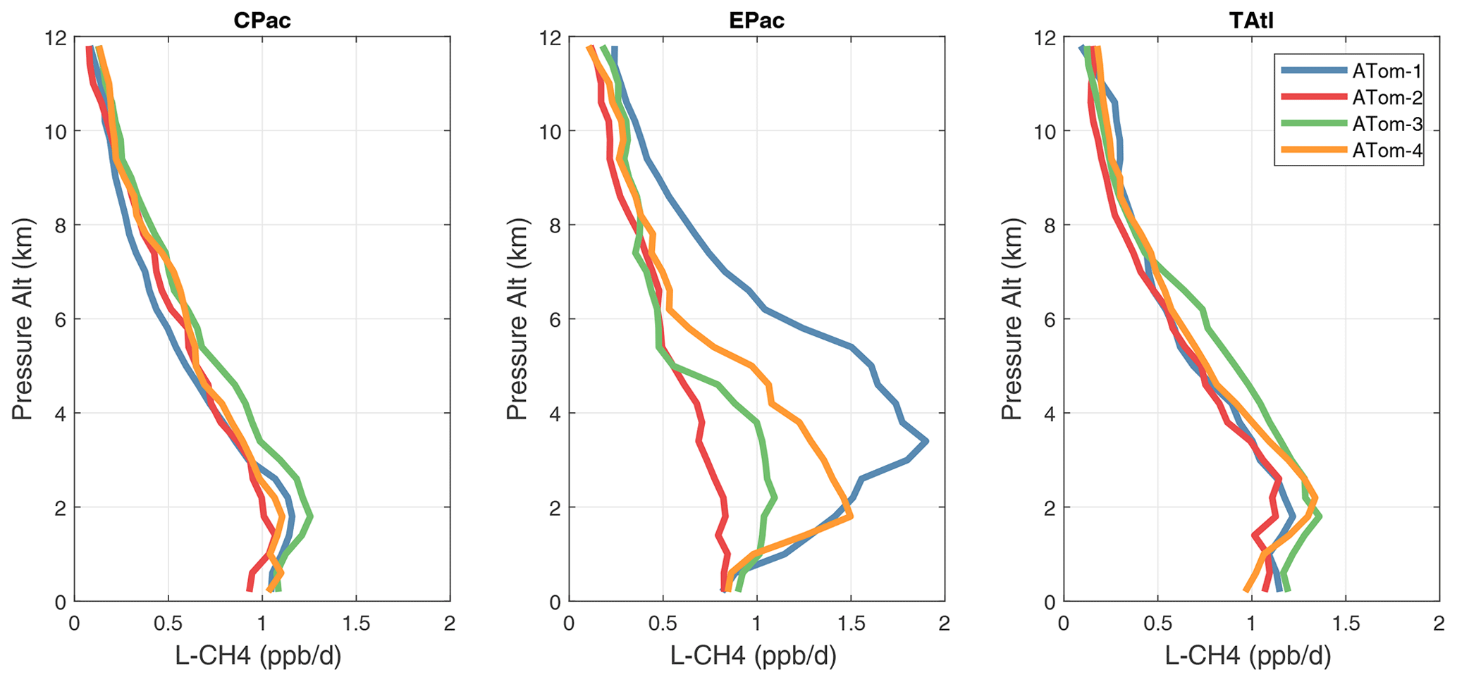
Figure 35 Mean altitude profile of L-CH4 (ppb d⁻¹) over the three tropical basins for ATom-1234.

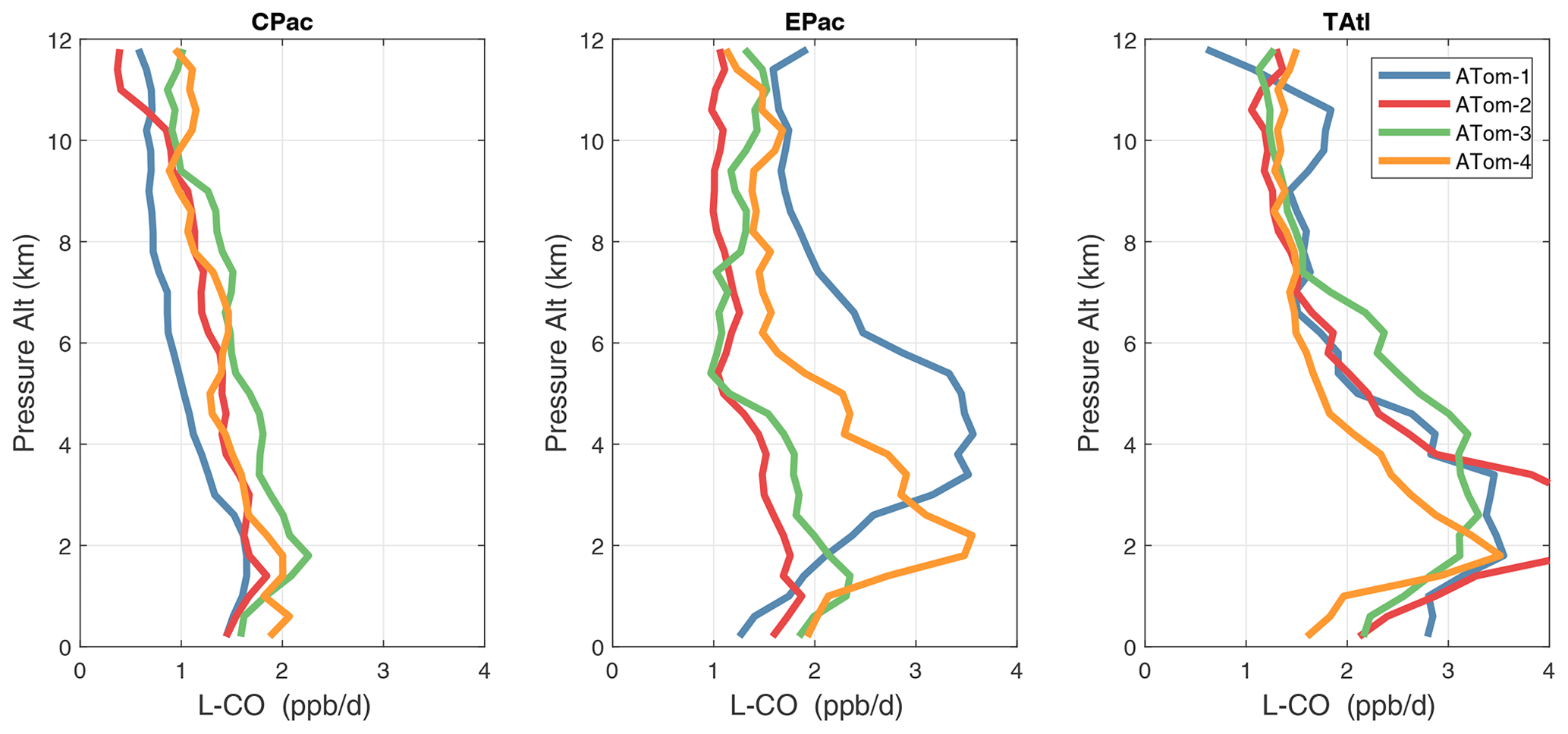
Figure 36 Mean altitude profile of L-CO (ppb d⁻¹) over the three tropical basins for ATom-1234.

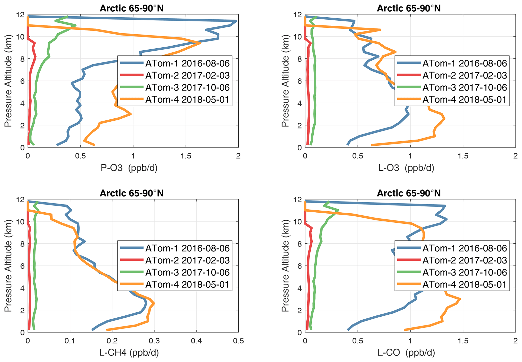
Figure 37 Mean altitude profile of the four reactivities (P-O3, L-O3, L-CH4, L-CO, ppb d⁻¹) over the Arctic (66–90^∘ N) for ATom-1234. All ATom 10 s parcels are weighted by the frequency of pressure sampling only. Troposphere-only parcels. Dates in the legend are the day of crossing the Equator in the Pacific for each deployment.

In the Antarctic (Fig. 38), reactivities are much lower than in the Arctic and are only reported for ATom-3; however, due to the limited sampling of the Antarctic, this may underestimate its role in the global or even regional budgets. The Southern Ocean reactivity profiles (Fig. 39) can be directly compared with the Arctic (Fig. 37) since both use the same axis scale. For L-CH4, they are almost identical (Southern Ocean ATom-23 and Arctic ATom-14), and the differences in L-CO are simply attributable to the smaller CO abundance in the Southern Hemisphere. The O₃ reactivities are much less in the Southern Ocean, however, and there is no peak in P-O3 (1–2 ppb d⁻¹) above 8 km as found in the Arctic. The Arctic clearly has much greater pollution in the upper troposphere, including possible aviation NO_x sources.

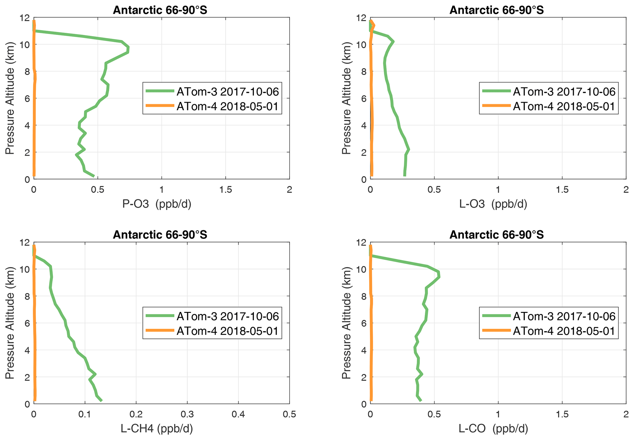
Figure 38 Mean altitude profile of the four reactivities (P-O3, L-O3, L-CH4, L-CO, ppb d⁻¹) over Antarctica on ATom-34. All ATom 10 s parcels are weighted by the frequency of pressure sampling only. Troposphere-only parcels. See Fig. 37.

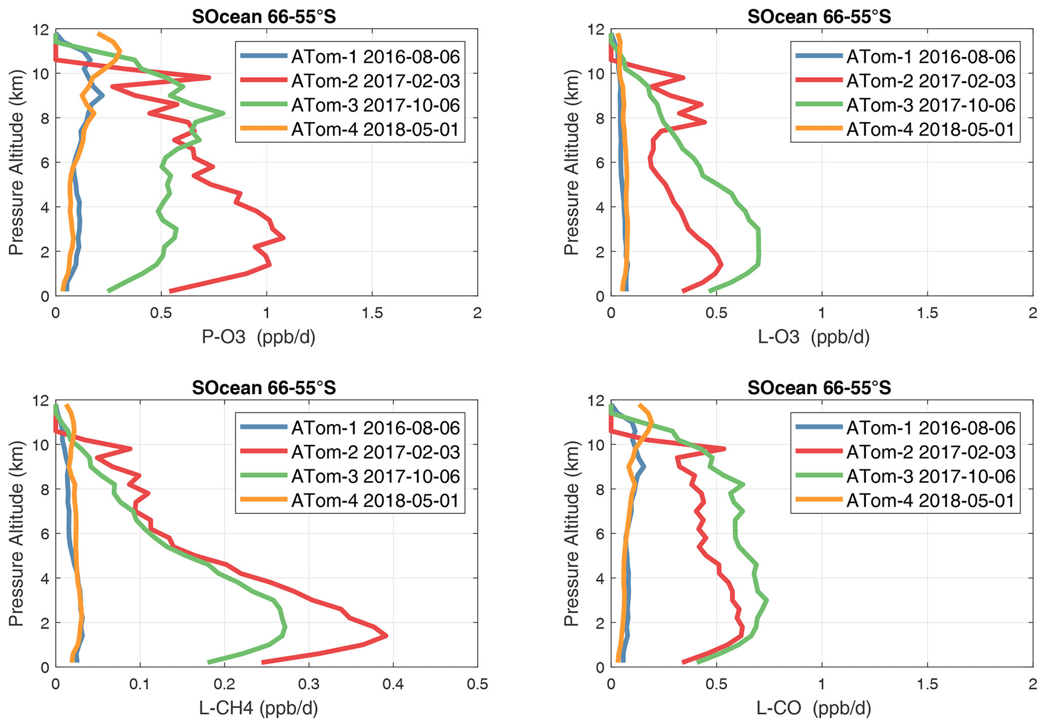
Figure 39 Mean altitude profile of the four reactivities (P-O3, L-O3, L-CH4, L-CO, ppb d⁻¹) over the Southern Ocean (66–55^∘ S) on ATom-1234. All ATom 10 s parcels are weighted by the frequency of pressure sampling only. Troposphere-only parcels. See Fig. 34.

3.4 Probability densities of photochemical reactivities

The probability densities (PDs) of the ATom reactivities have proven useful in testing model climatologies (see G2023) and are shown for the Pacific and Atlantic basins and the four reactivities in Figs. 40–43. All four deployments are shown in each panel. The relatively low P-O3 PD stands out for both the Pacific and Atlantic. The L-CH4 PD peaks at the lowest value, with a secondary peak above 1 ppb d⁻¹. The very low values of L-CH4 simply reflect the sampling of the upper troposphere, where the OH + CH₄ rate coefficient proportional to exp($-\mathrm{1775}/T$) is very small. Thus, the L-CO PD, which is also proportional to OH, peaks at higher values. Restricting our PDs to the three tropical regions (Figs. 44–47), we find some distinct deployments (e.g., low P-O3 in the central Pacific for ATom-1, high P-O3 in the tropical Atlantic for ATom-3, and high L-CH4 in the eastern Pacific for ATom-1), but for the most part the reactivity PDs present similar patterns for each reactivity in each tropical basin. Thus, the ATom PDs provide a useful climatology for model comparisons.

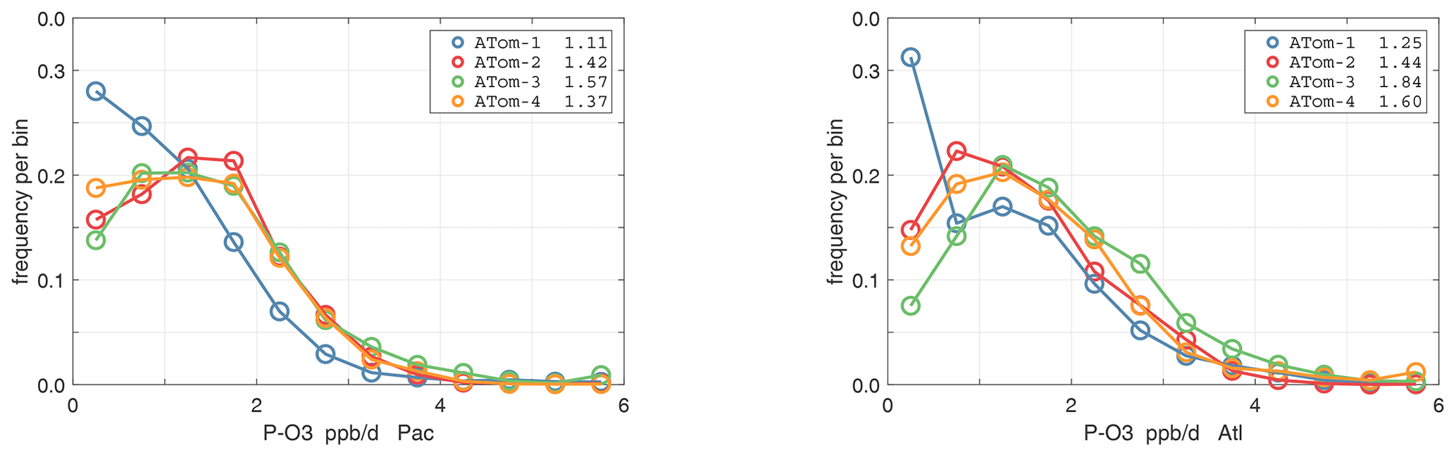
Figure 40 Probability density of P-O3 (ppb d⁻¹) in the Pacific and Atlantic basins (53^∘ S–60^∘ N) for ATom-1234. Values in the legend are the basin-wide weighted averages for each deployment. The frequency of parcels with reactivities greater than the maximum shown are added to the last point.

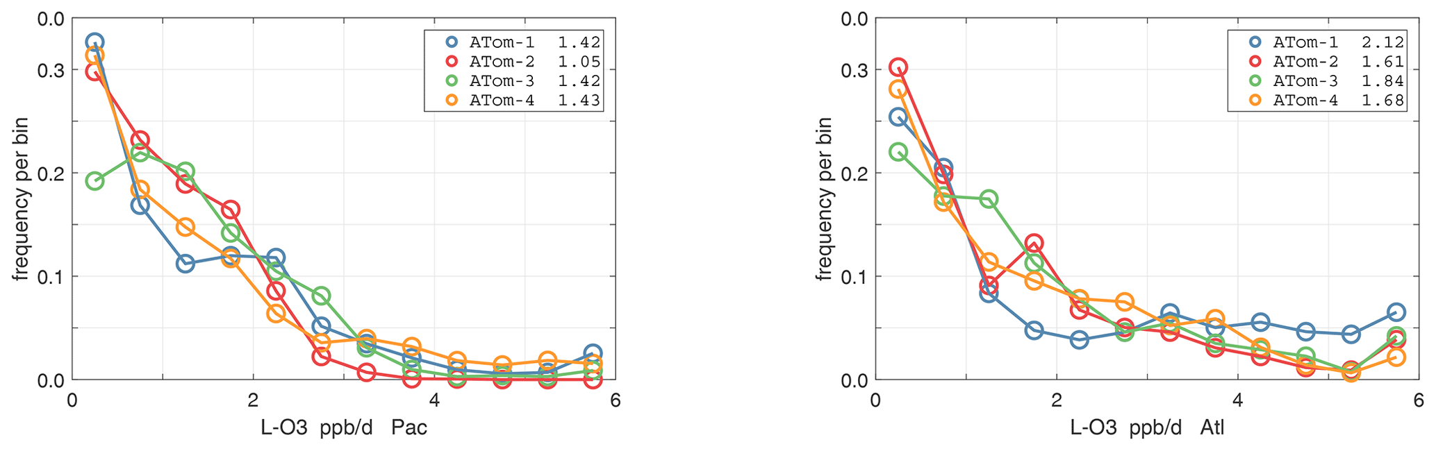
Figure 41 Probability density of L-O3 (ppb d⁻¹) in the Pacific and Atlantic basins for ATom-1234. See Fig. 40.

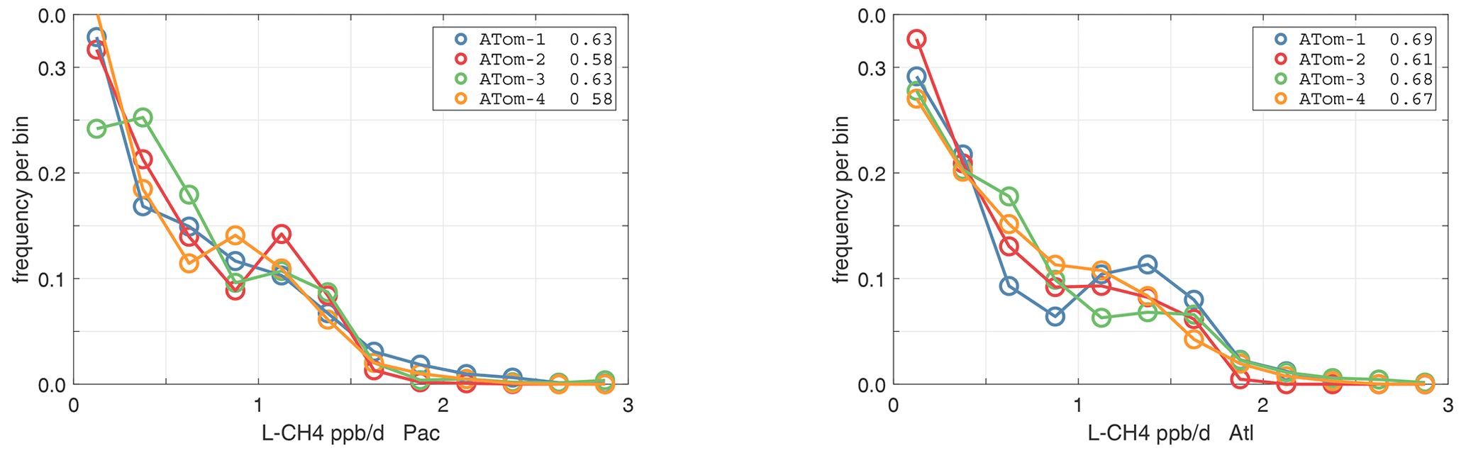
Figure 42 Probability density of L-CH4 (ppb d⁻¹) in the Pacific and Atlantic basins for ATom-1234. See Fig. 40.

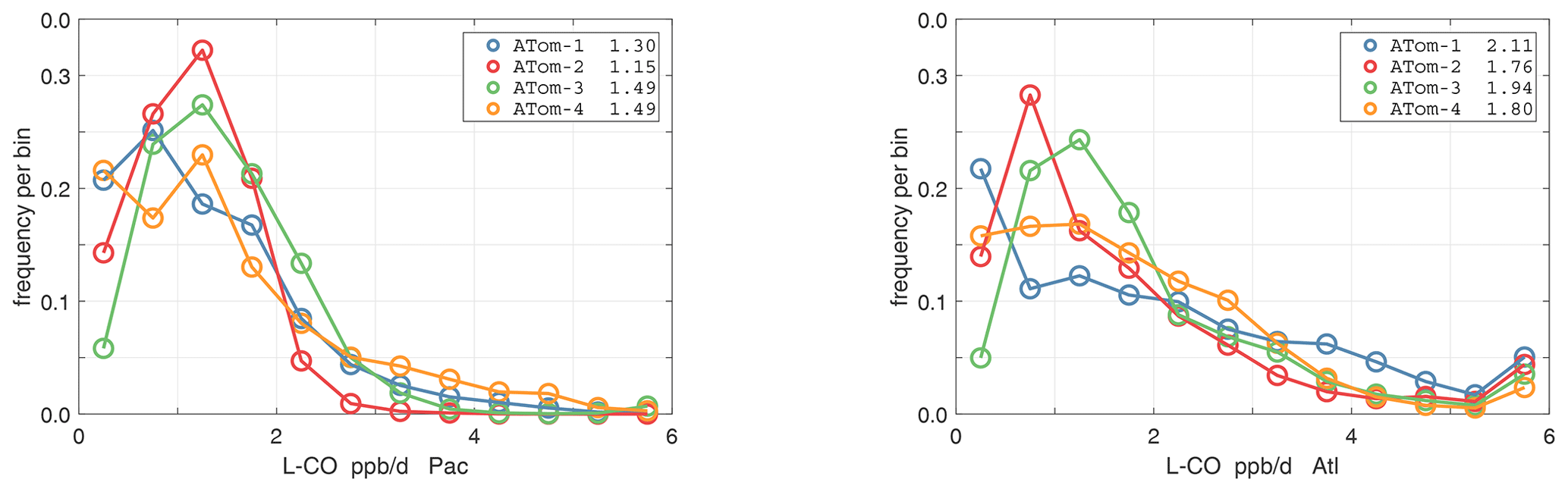
Figure 43 Probability density of L-CO (ppb d⁻¹) in the Pacific and Atlantic basins for ATom-1234. See Fig. 40.

4 Chemical sensitivity analysis

4.1 First-order sensitivities

To identify the critical species controlling the tropospheric budgets of O₃ and CH₄, we calculate the sensitivity of the weighted mean reactivity for the Pacific or Atlantic oceanic flights of ATom-1 (53^∘ S to 60^∘ N) with respect to the species measured by ATom. Sensitivity analyses are often calculated with CCMs to assess the factors controlling the trends and variability in CH₄ lifetime (Holmes et al., 2013). With CCMs, the calculation includes emissions, scavenging, transport, and chemistry, but here using ATom observations we are limited to a 24 h snapshot with only the chemical evolution of the parcels. We believe that this limitation does not affect our goal of estimating the errors in the modeled budgets caused by errors in the modeled values of the critical species.

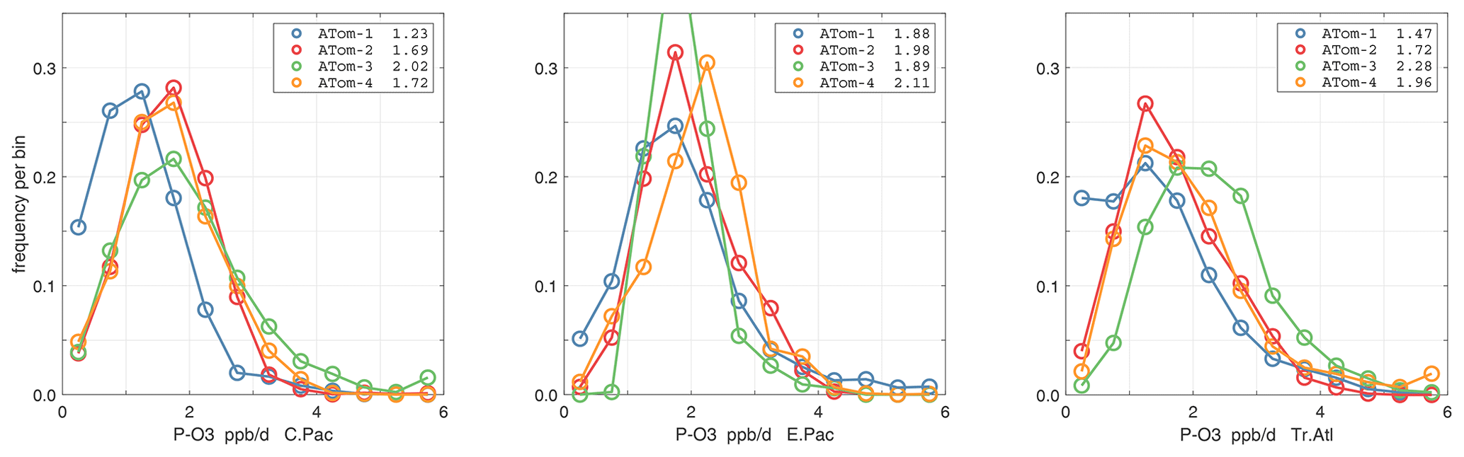
Figure 44 Probability density of P-O3 (ppb d⁻¹) in the three tropical basins (30^∘ S–30^∘ N) for ATom-1234. See Fig. 40.

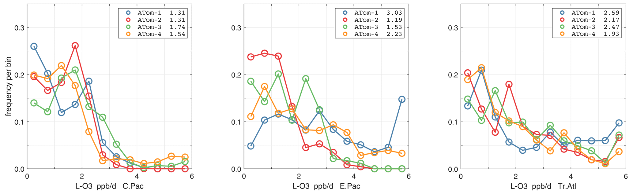
Figure 45 Probability density of L-O3 (ppb d⁻¹) in the three tropical basins for ATom-1234. See Fig. 40.

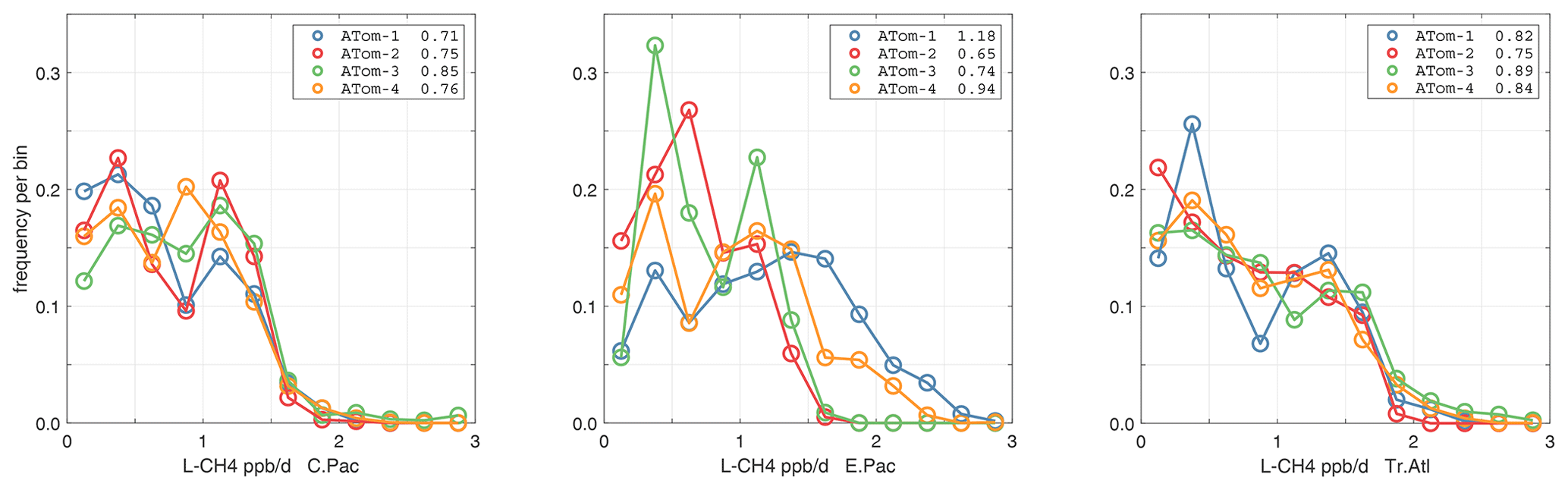
Figure 46 Probability density of L-CH4 (ppb d⁻¹) in the three tropical basins for ATom-1234. See Fig. 40.

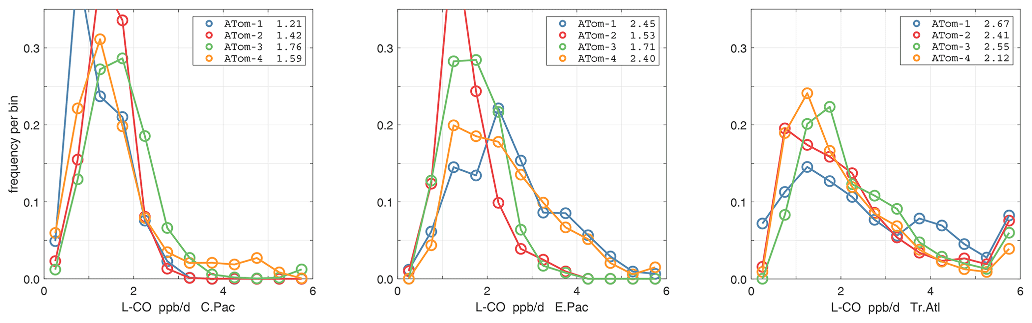
Figure 47 Probability density of L-CO (ppb d⁻¹) in the three tropical basins for ATom-1234. See Fig. 40.

The sensitivity S of reactivity R to species X is calculated from the fractional change in R per fractional change in X (dimensionless, e.g., percentage per percentage). We use Δ=10 %.

$$\begin{array}{}\text{(1)}& S\equiv {\displaystyle \frac{\mathrm{d}\left\{\ln \left(R\right)\right\}}{\mathrm{d}\left\{\ln \left(X\right)\right\}}}={\displaystyle \frac{\ln (R\left[X\cdot \left(\mathrm{1}+\mathrm{\Delta }\right)\right]/R[X\left]\right)}{\ln (\mathrm{1}+\mathrm{\Delta })}}\end{array}$$

Results from 20 variables (19 chemical species plus T) for the four reactivities over the Pacific and Atlantic basins for ATom-1 are given in Table 2. The mean sensitivities are calculated using basin-wide averages and have only been calculated using one day's cloud fields (day 223) instead of the five days of different cloud fields (e.g., days 213, 218, 223, 228, or 233) used for the reactivities in Sect. 3. Basin-mean differences between two separated days (days 213 and 223) due to cloud fields and ozone columns are evaluated and found to be small: < 1 % of the value of S or smaller than 0.002 in absolute value. Thus, evaluating S with one day is adequate.

Individual parcels show highly variable individual S values (see the examples in Fig. 48). The scatter is particularly large because we have included all the ATom-1 parcels, including continental data and very low sun angles. For comparison, the basin-mean values (large blue and red dots) are also plotted. Differences across basins and deployments are modest (not shown), and the Pacific–Atlantic comparison for ATom-1 covers this range, remembering that ATom-1 Pacific has unusually low P-O3 values. Surprisingly, the initial values of many species have a negligible or small impact on the reactivities. Species like alkanes and alkenes are unimportant because their average abundances are low over the oceans, and species like HCHO and HNO₄ are unimportant because their abundances are reset by the chemistry during the 24 h integration.

The lessons from Table 2 are quite interesting. (i) T, H₂O (Q), and O₃ are absolutely critical for all the chemical budgets. (ii) NO_x is critical for P-O3 but less so for L-CH4 and L-CO and even less so for L-O3. (iii) CO as expected controls OH and L-CH4. (iv) CH₄ is like CO but plays a bigger role in P-O3 through HO_x production via HCHO. (v) HOOH plays a modest role (S∼ 0.06) in OH and thus L-CH4 and L-CO. (vi) CH₃OOH plays a surprisingly large role in P-O3 because of the additional HO_x release through HCHO. However, (vii) the initial HCHO plays a small role in P-O3 because it is reset quickly by the chemistry in response to the other species listed here. PAN and HNO₃ contribute noticeably to P-O3 through their slow decomposition to NO_x. Acetaldehyde (CH₃CHO) stands out in reducing P-O3, L-CH4, and L-CO, presumably from NO_x to PAN conversion, with S ranging from −0.05 to −0.09.

One of the most interesting features of Table 2 is the impact of O₃ on its net P-O3 minus L-O3. With O₃ increases, the sum of reactions going into L-O3 increases almost linearly, while the P-O3 reactions decrease. Thus, the net sum decreases more quickly than linearly. The implications of this for the lifetime of O₃ perturbations is discussed with chemical feedbacks in Sect. 6.

Table 2 Sensitivities ($S=\mathrm{dln}\left[R\right]/\mathrm{dln}\left[X\right]$, dimensionless) for ATom-1.

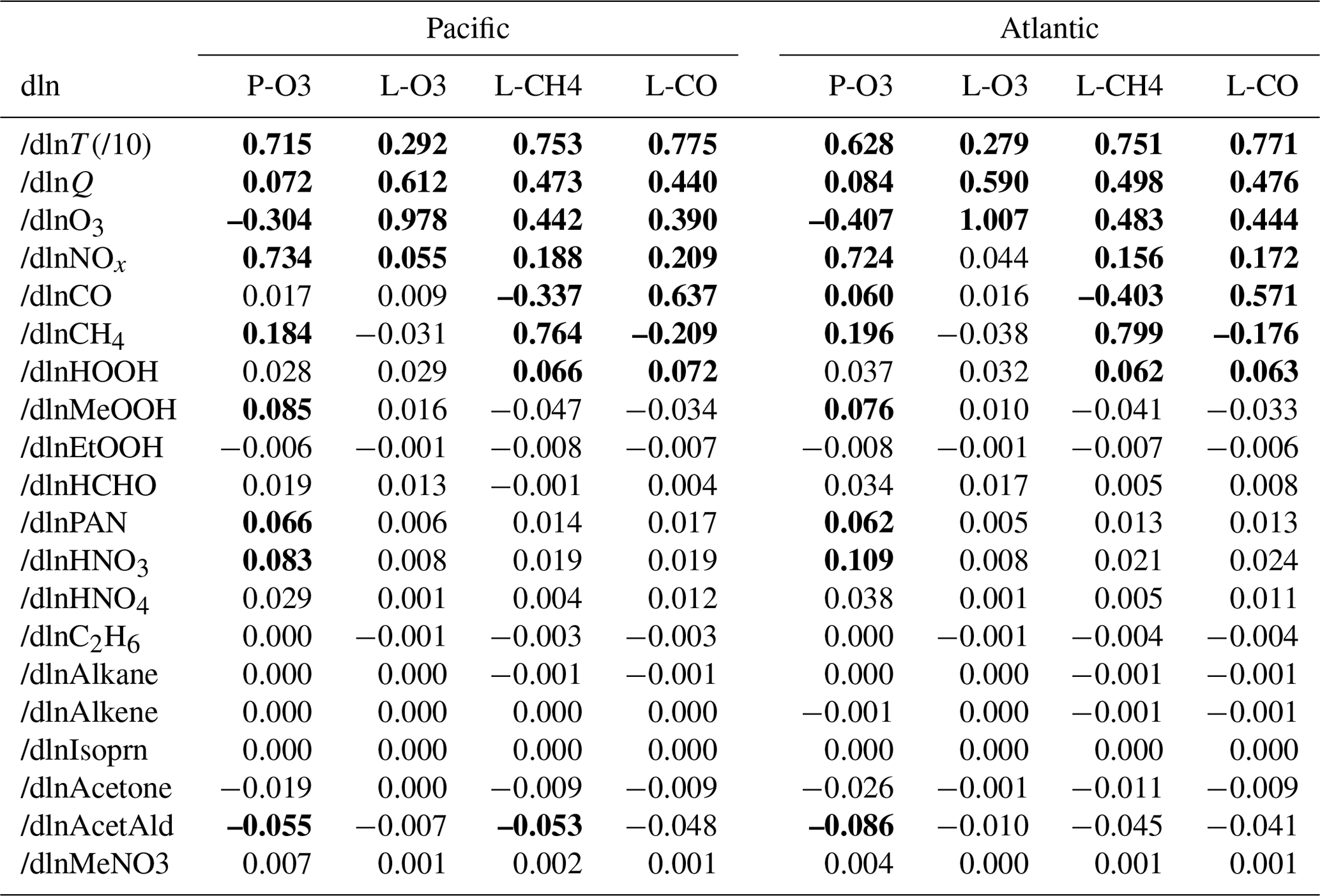
Sensitivities are calculated as $S=\mathrm{dln}\left[R\right]/\mathrm{dln}\left[X\right]$ (percentage per percentage) with a 10 % perturbation being applied to all 10 s parcels. Q is H₂O and was perturbed 10 % like all the chemical species. T is an exception, with a 1 % perturbation being used, and thus $\mathrm{dln}\left[R\right]/\mathrm{dln}\left[T\right]$ should be multiplied by 10 to get the percentage per percentage. Sensitivities that would round to $\left|S\right|$ > 0.1 are shown in bold. The average sensitivity over the basin is calculated here from (a) the single basin-wide average of R. Alternative but less desirable methods would average the individual parcel S values weighted by (b) frequency of occurrence and the R value or (c) just frequency of occurrence. Methods (a) and (b) are very close but are not identical, while method (c) is clearly different. For any of the large S values ($\left|S\right|>\mathrm{0.1}$), the differences between (a) and (b) are < 1 %, except for dln[P-O3]/dln[T]. As an example, the (a), (b), and (c) values in the Pacific are 0.715, 0.694, and 0.811 for dln[P-O3]$/$dln[T]$(/\mathrm{10})$, 0.764, 0.764, and 0.796 for dln[L-CH4]$/$dln[CH₄], and −0.304, −0.305, and −0.311 for dln[P-O3]$/$dln[O₃].

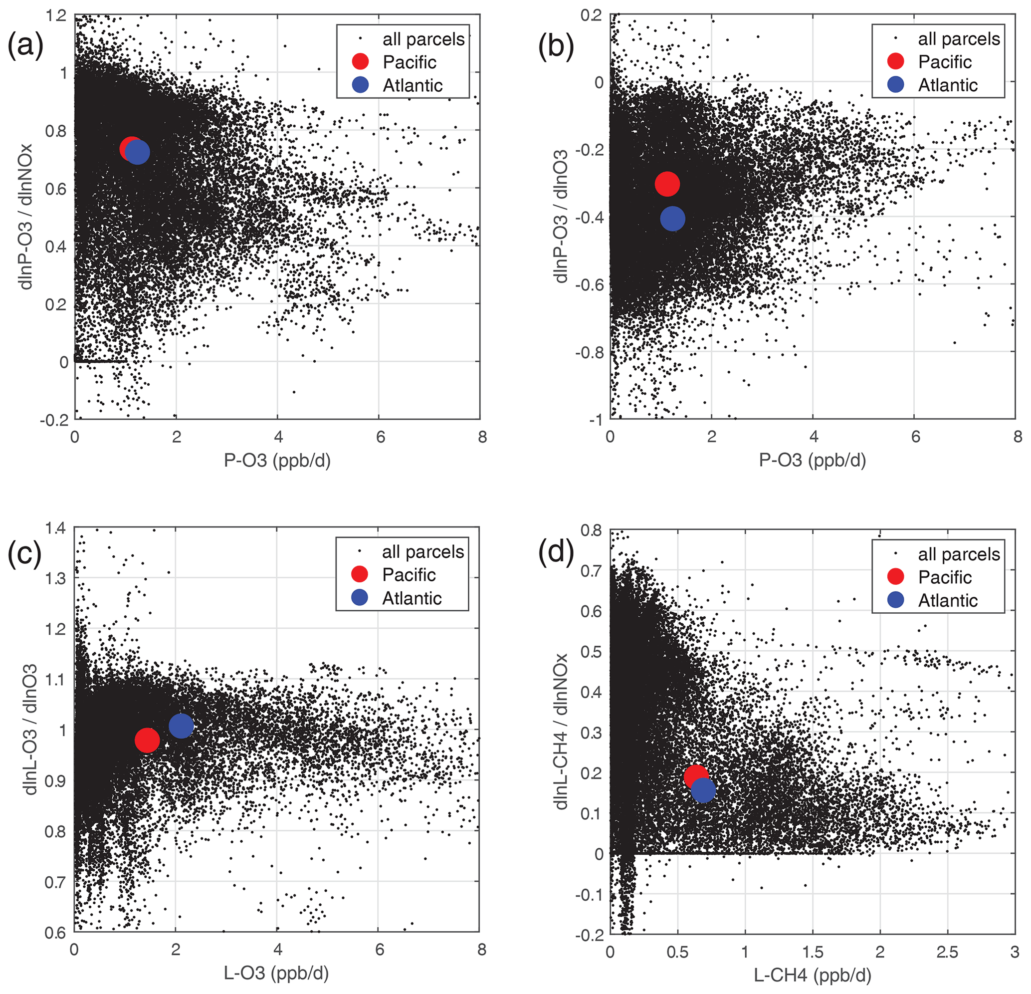
Figure 48 Sensitivity (percentage per percentage) plotted against reactivity (ppb d⁻¹) for ATom-1: (a) dln[P-O3]$/$dln[NO_x], (b) dln[P-O3]$/$dln[O₃], (c) dln[L-O3]$/$dln[O₃], and (d) dln[L-CH4]$/$dln[NO_x]. All ATom-1 parcels, including continental data, are plotted as small black dots; the basin-mean values for the Pacific as large red dots; and the Atlantic as large blue dots.

4.2 Second-order terms

Considering that most chemical reactions are of the forms R=k(T)XY or k(T)X², we should evaluate the second-order terms in the Taylor expansion. We first tested the quadratic nature of our S values by recalculating with Δ=20 %, but the results hardly changed, and so we are in a linear regime. The second-order cross-species terms are potentially more interesting. We calculate these from a coupled 10 % perturbation of two different variables.

$$\begin{array}{}\text{(2)}& \begin{array}{rl}{S}_{XY}& \equiv S\left(X+\mathrm{10}\mathit{\%},Y+\mathrm{10}\mathit{\%}\right)-S\left(X+\mathrm{10}\mathit{\%},Y\right)\\ & -S\left(X,Y+\mathrm{10}\mathit{\%}\right)\end{array}\end{array}$$

We calculated these cross terms only for X= O₃, NO_x, CO, CH₄, Q, and T, using ATom-1 only as in Table 2. Table 3 shows the deviations from linearity (S_XY) for each of the 15 XY pair combinations, listing the Pacific basin in the upper triangular part of the matrix and the Atlantic basin in the lower triangular part. The diagonals simply give the mean first-order S_X values for the Pacific plus the Atlantic. These off-diagonal S_XY terms are clearly second order in importance for the chemistry: e.g., the importance of the S_XY term in d²ln(L-CO)$/$dln(O₃) dln(Q) for the Pacific is given as +0.017, which is a small fraction of the first-order terms of +0.42 for dln(L-CO)$/$dln(O₃) and +0.46 for dln(L-CO)$/$dln(Q). The near symmetry of the four matrices in Table 3 indicates that average S_XY sensitivities are similar for both basins. Hence we find no evidence that coupled perturbations must be considered when modelers explore the factors driving changes in the lifetime of CH₄ (e.g., Holmes et al., 2013).

Although we have long known that H₂O and T are important factors (e.g., Table 2 of Holmes et al., 2013), these quantities have often been relegated to the physical climate system and are not often thought of a major source of model error in the chemical system. Thus, when we diagnose the future tropospheric O₃ or CH₄ from the multi-model comparisons (Stevenson et al., 2013; Voulgarakis et al., 2013; Young et al., 2018; Griffiths et al., 2021), we need to document biases in T and H₂O. For example, from Thornhill et al. (2021a), we estimate an increase in the CH₄ loss frequency of about 4.5 % K⁻¹ for the two consistent models. (The other two models in the Thornhill study each seem aberrant in their own way.) From Table 4, a +1 K change increases L-CH4 by 2.5 %, and the Clausius–Clapeyron-inferred 7 % increase in Q adds 3.4 % for a total of 5.9 % K⁻¹, a reasonable first-order result considering that other climate-driven changes, such as O₃, are not included. For model evaluation, comparing T with mean profiles is straightforward, but H₂O is more difficult, even with profiles, because of the 3 orders of magnitude change over the troposphere. Thus, we recommend that relative humidity over liquid water (RH_w, %) be used to detect bias. See the statistics on critical species and RH_w in the next section.

Table 3 Second-order cross-term sensitivities S_XY calculated as S(+dX+dY) − S(+dX) − S(+dY) for the Pacific (upper-triangular) and Atlantic (lower-triangular) basins in ATom-1.

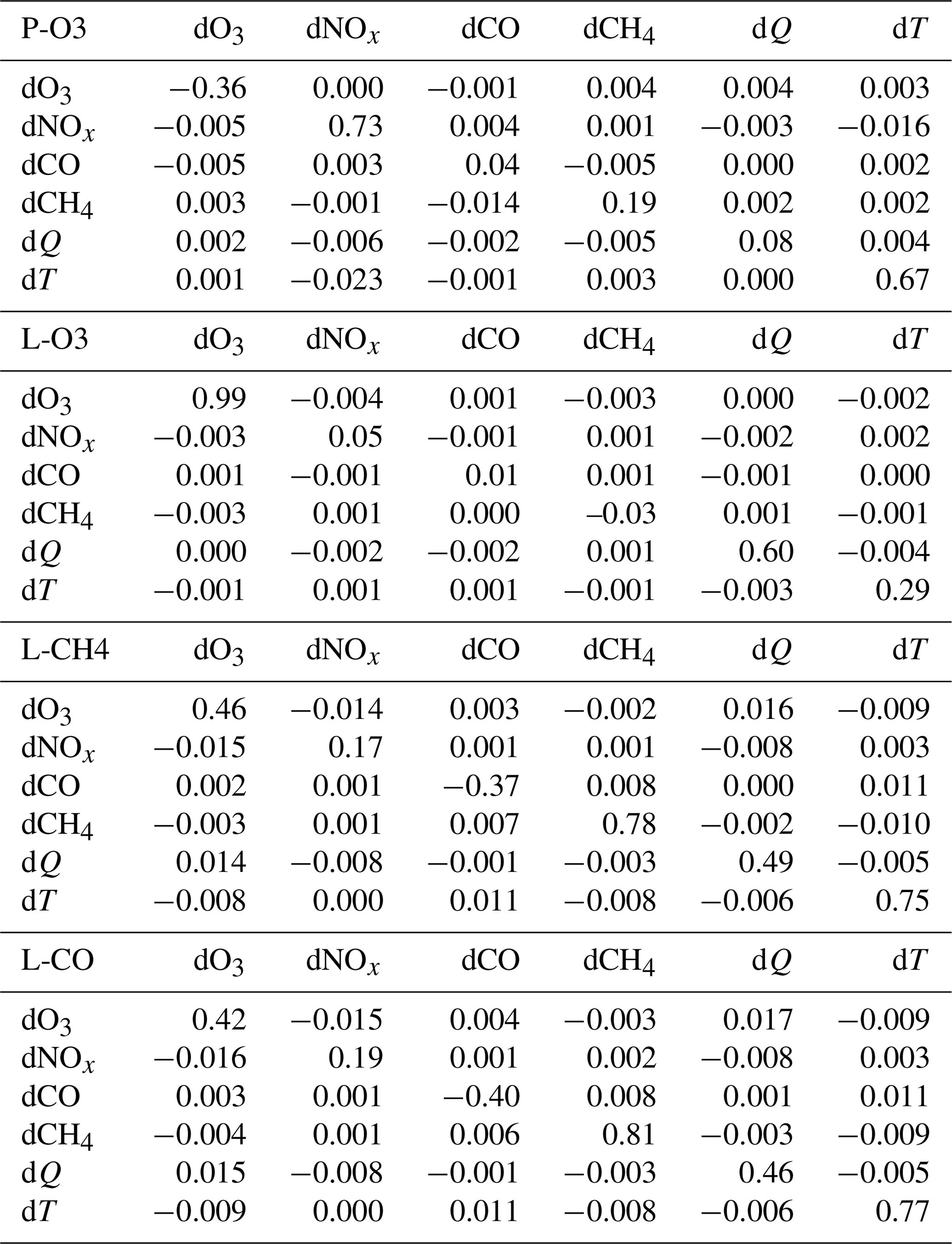
T is temperature and was perturbed only 1 %. Q is H₂O and was perturbed 10 % like all the chemical species. The diagonal elements are the average (Pacific and Atlantic) first-order sensitivities S(+dX) (see Table 2). The upper-triangular (Pacific) and lower-triangular (Atlantic) matrices show the second-order sensitivities S_XY=S(+dX+dY) − S(+dX) − S(+dY).

5 Key ATom species and NO_x version 3

5.1 NO_x version 3 and MDS flags

When completing this paper's analysis of the reactivities (Sect. 3) and re-examining the problems with NO_x (NO₂+ NO) profiling that led to MDS version 2b (described in G2023), we re-examined the NO_x long-gap interpolation. There were long stretches of these gaps (flag = 4) and missing flight data (flag = 5) that resulted in critical flight segments being filled with mean profile data. These gaps are caused by the lack of NO₂ rather than NO measurements as shown in Fig. 49 (four ATom deployments multiplied by two ocean basins). The number of profiles with NO data but no NO₂ data (red dots) is extensive and covers some key regions (e.g., the lower troposphere in the Atlantic in ATom-2 or the eastern Pacific in ATom-34). Thus, we developed a secondary measurement of NO_x (flag = 2) based on the measured value of NO.

We look for a linear relationship between NO_x and NO, i.e., [NOx^fit] = A [NO], and use the Pacific Ocean and Atlantic Ocean basins to avoid continental pollution. Adding a multiplier of [O₃], the right-hand side did not improve the fit. The ratio A does not depend noticeably on altitude. A linear fit of A minimizing the errors, NOx^fit - NO_x, for oceanic NO_x values < 250 ppt gives A=2.055. The unweighted mean value of NO_x is 50 ppt, the 1 sigma range of errors (16th–84th percentiles) is ±22 ppt, and the RMSE is 31 ppt. Figure 50 shows the oceanic NOx^fit points (red) and all others (blue) plotted against NO_x. The new 8400 NOx^fit parcels are labeled with flag = 2 and eliminate most of the long-gap parcels and all of the missing flight parcels. The G2023 Table S4 percentage of flags = 0-1-2-3-4-5 for NO_x changes from 0.8 %-80.8 %-0.0 %-8.3 %-7.6 %-2.5 % to 0.8 %-80.8 %-5.7 %-8.7 %-4.0 %-0.0 %. This new NOx^fit is named “NOxadd” in version 3 of the MDS (ATom_MDS3.nc). In this paper the figures with the new version-3 NOx^fit are labeled NOxx.

Caution should be taken when using the MDS data for observational statistics because of the gap-filling needed to calculate the RDS. MDS data flagged with 1 or 2 are reliable because they are based on primary or secondary instrument observations. Short-gap interpolation (flag = 3) has been tested (G2023) and found to be reasonably accurate. Further, adding a short-gap, linearly interpolated flight segment (< 1 km in altitude) will have little effect on species statistics here because of the parcel weighting that is used to achieve equal sampling with altitude and latitude. Flags 4, 5, and 6 are more worrisome as these long-gap or missing-flight methods cannot be evaluated for accuracy. In MDS v3, the chemical species with > 10 % of parcels with flags 4, 5, and6 are HNO₄, CH₃OOH, C₂H₆, alkanes, C₂H₄, alkenes, C₂H₂, all alkyl nitrates, and SF₆. Fortunately, the only one of these species that has a significant impact on the RDS ($\left|S\right|\sim$ 0.1) is CH₃OOH.

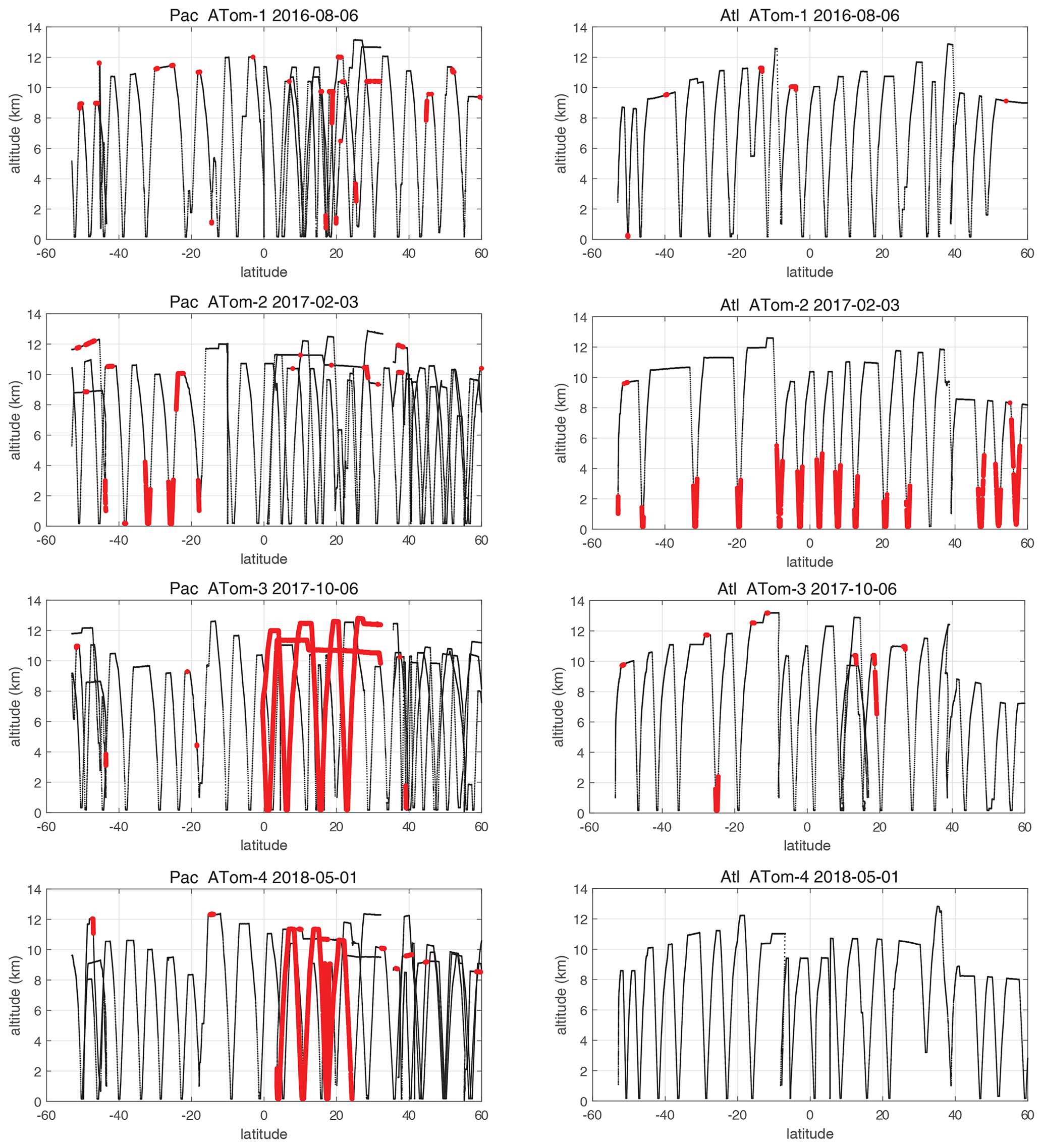
Figure 49 ATom-1234 profiling in the Pacific and Atlantic basins showing parcels (large red dots) where NO₂ observations are missing, where long-gap interpolation was used in MDS version 2b, and where shifting to NOx^fit based on NO observations in MDS version 3 results in a change in NO_x of > 1 ppt.

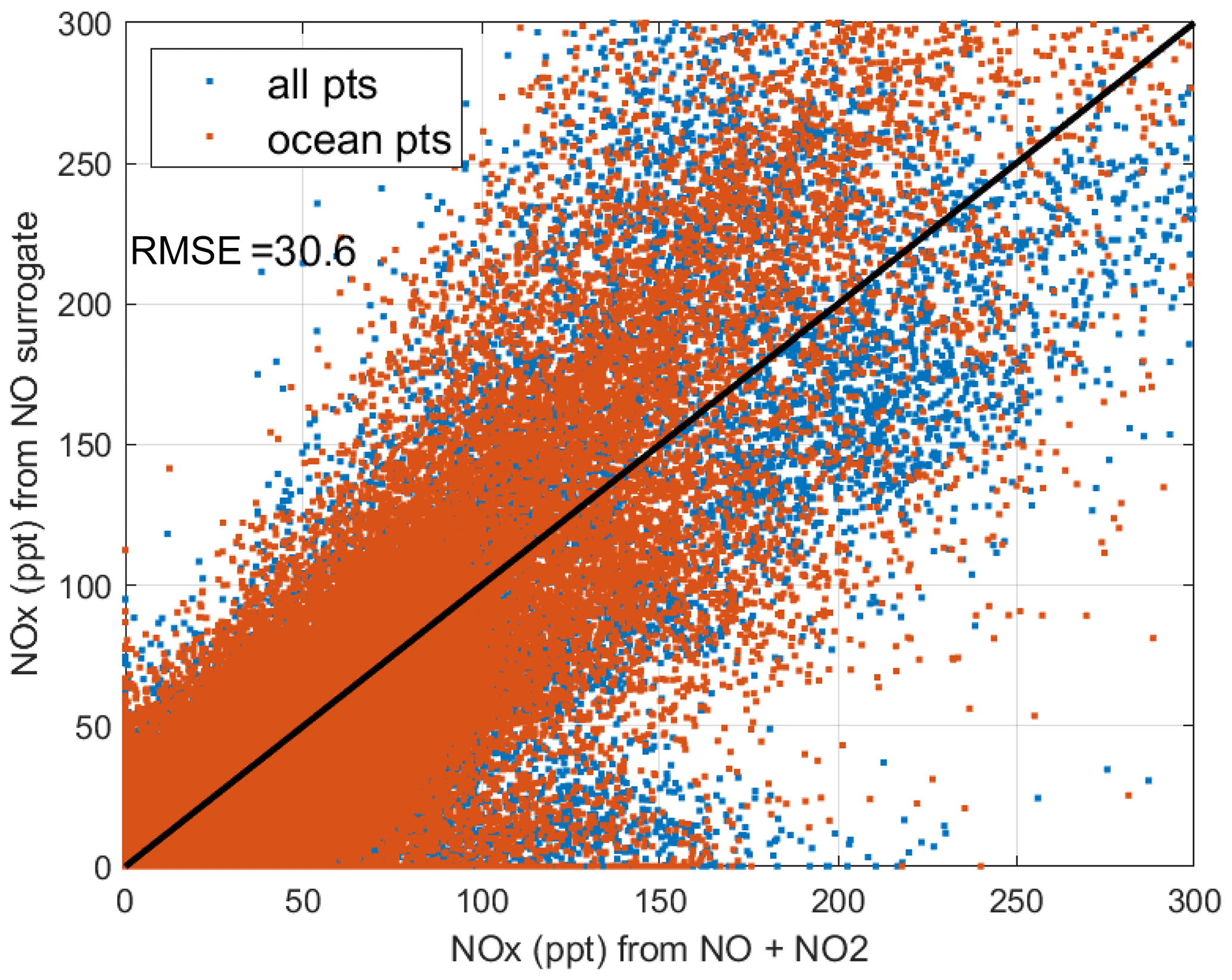
Figure 50 Scatter plot of NO_x using NO as a surrogate (NO${}_x=\mathrm{2.055}\times$ NO, y axis) and directly measured NO_x (x axis) for all ATom parcels where NO₂ is measured. The red points are all the ocean basin parcels, and the blue points are all the others. The 1:1 black line is for reference.

5.2 Updated version-3 reactivities

We did not have the resources to repeat all the calculations (5 d averages, sensitivities) with version-3 NO_x and so choose to redo all reactivity calculations with just the first day in each deployment (i.e., days 32, 121, 213, and 274). Comparisons of reactivities must then be done with the same single-day calculation with version 2b. Given the range in reactivities for ATom-1 Pacific and Atlantic, we also did not redo the sensitivities for MDS-3. Table 4 provides a summary of the changes in Pacific and Atlantic basin-mean and median reactivities for ATom-1234 calculated using only the first day. Almost all the changes from v2b to v3 are negative. P-O3 has, as expected, the largest changes for ATom-3 Pacific and ATom-2 Atlantic. Here the median decrease (−13 % and −16 %, respectively) is twice as large as the mean, implying a large shift in the mid-level values of P-O3. The remaining changes in the mean reactivities are small, 0 % to −3 %.

Vertical profiles of the four mean reactivities are shown in Figs. 51–54, with separate panels for the Pacific and Atlantic basins and ATom-1234 shown in each panel. The solid colored lines are calculated for one day with v3 NOx^fit, and the dashed colored lines are calculated for v2b NO_x. For P-O3, the difference is visible at different altitudes for ATom-234, but the profile shape is clearly changed for ATom-3 Pacific 10–12 km and ATom-2 Atlantic 0–2 km. Remembering that only NO_x changes here with v3 and that P-O3 has the highest sensitivity to NO_x, we expect the other reactivities (L-O3, L-CH4, L-CO) to change little. This is the case except for L-CH4 and L-CO for ATom-2 Atlantic 0–2 km.

Table 4 Reactivity change (%) from MDS v2b to v3.

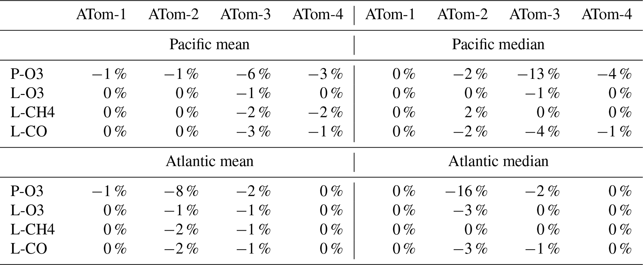
Unweighted mean of all the parcels, calculated for day 1 only and not averaged over 5 separate days.

The PDs for the reactivities in each ocean base are shown in the eight panels of Fig. 55. The weighted mean reactivities (ppb d⁻¹) in each basin are given for ATom-1234 in the figure legend, with the v2b value followed by the v3 value. The PDs and mean values here are for 1 d only and thus differ slightly from the 5 d averages analyzed in Sect. 3. Similarly to the profiles, the PDs show detectable but insignificant changes from v2b to v3 and remain robust (i.e., compared with Figs. 40–43). For the most part, the mean reactivities change by < 0.01 ppb d⁻¹, with major exceptions for P-O3 in Pacific ATom-34 and Atlantic ATom-23, where the v3 value is 0.03 to 0.10 ppb d⁻¹ smaller than the v2b value. The L-CO also shows some decreases with v3 of about 0.03 ppb d⁻¹ (Pacific ATom-3, Atlantic ATom-2), and in a relative sense (∼ 2 %) this might be true for L-CH4, but this is not apparent with the precision shown given that L-CH4 is 2–3 times smaller than L-CO.

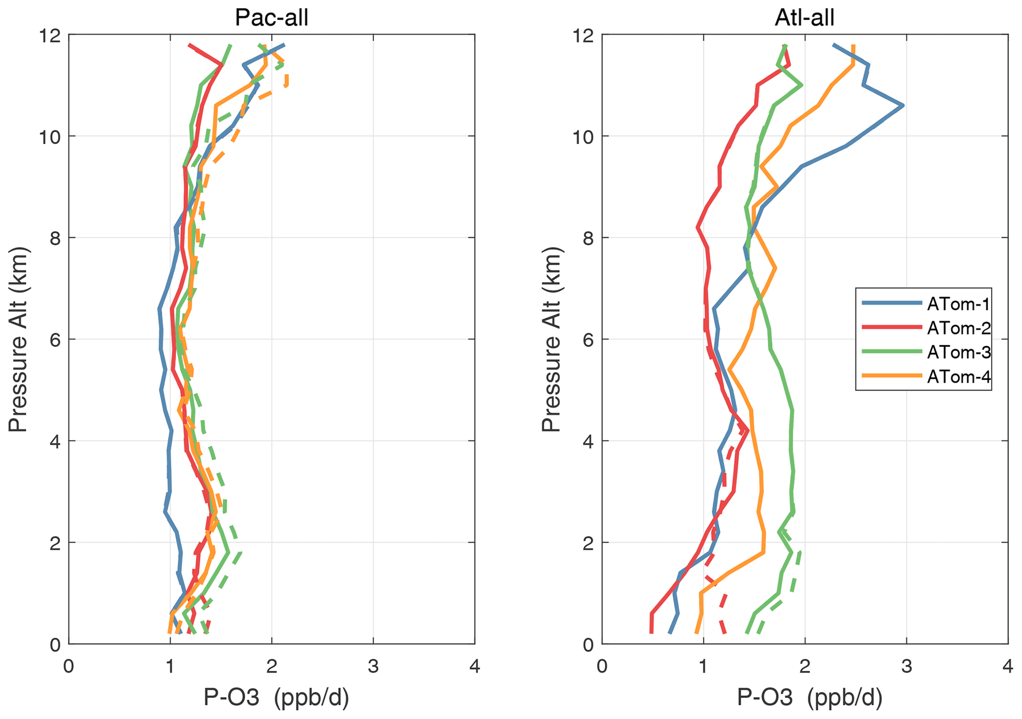
Figure 51 Altitude profiles of mean P-O3 (ppb d⁻¹) over the Pacific and Atlantic basins for ATom-1234. Results are for 1 d only in each deployment (days 32, 121, 213, and 274). Compare with Fig. 29. The solid lines are for version-3 NO_x, and the dashed lines are for version 2b.

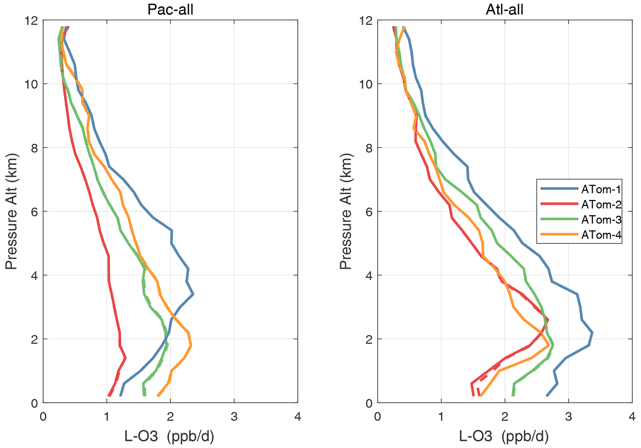
Figure 52 Altitude profiles of the mean L-O3 (ppb d⁻¹) over the Pacific and Atlantic basins for ATom-1234. See Fig. 51. Compare with Fig. 30. Solid lines are MDS-3, and dashed lines are MDS-2b.

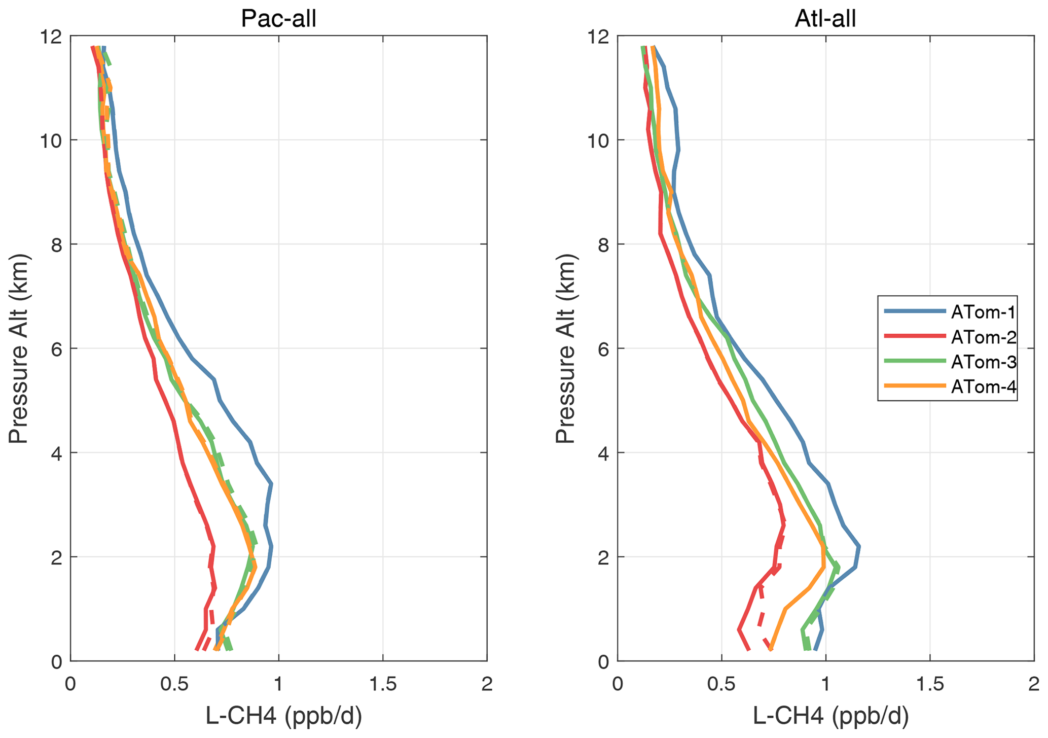
Figure 53 Altitude profiles of the mean L-CH4 (ppb d⁻¹) over the Pacific and Atlantic basins for ATom-1234. See Fig. 51. Compare with Fig. 31. Solid lines are MDS-3, and dashed lines are MDS-2b.

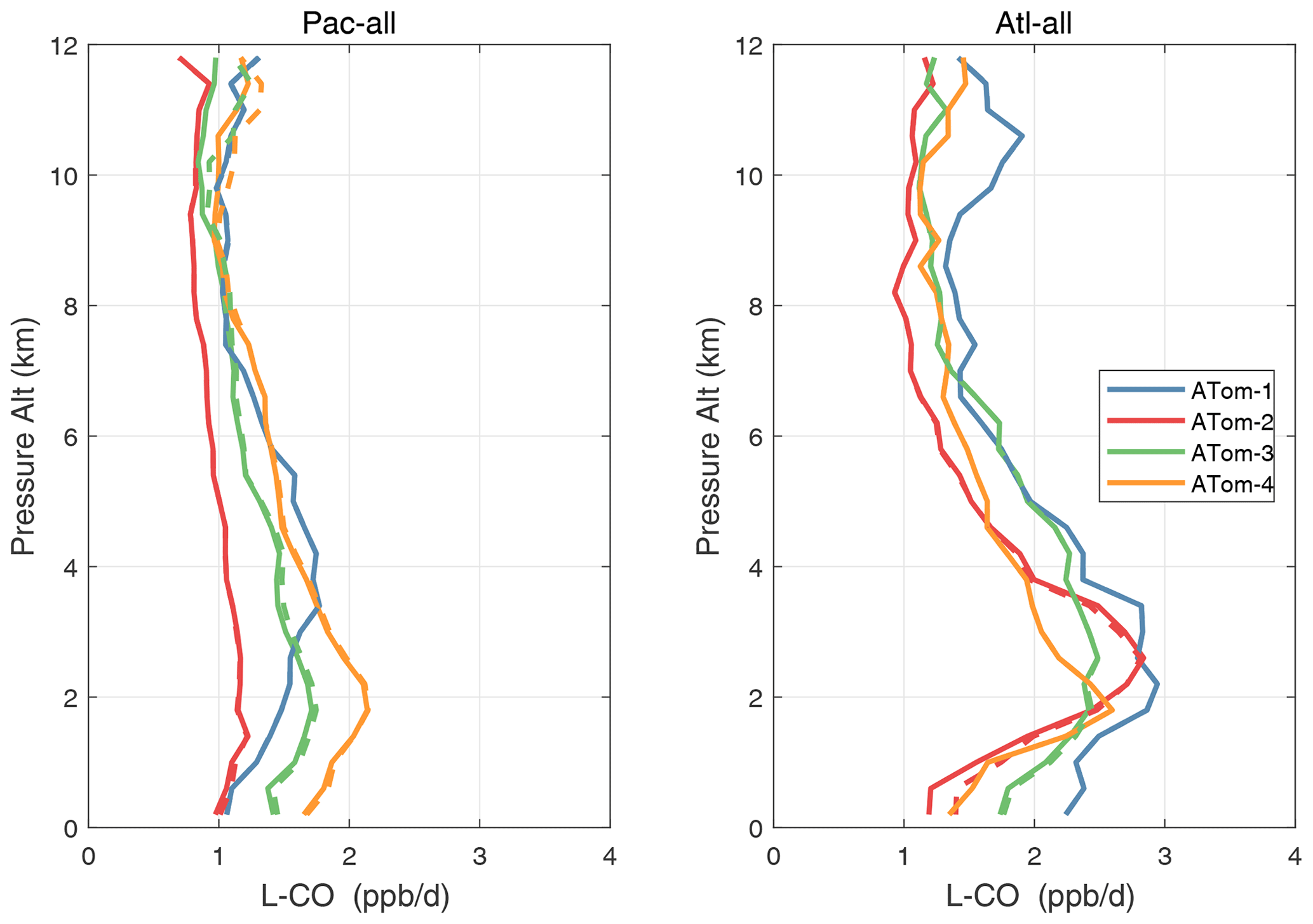
Figure 54 Altitude profiles of the mean L-CO (ppb d⁻¹) over the Pacific and Atlantic basins for ATom-1234. See Fig. 51. Compare with Fig. 32. Solid lines are MDS-3, and dashed lines are MDS-2b.

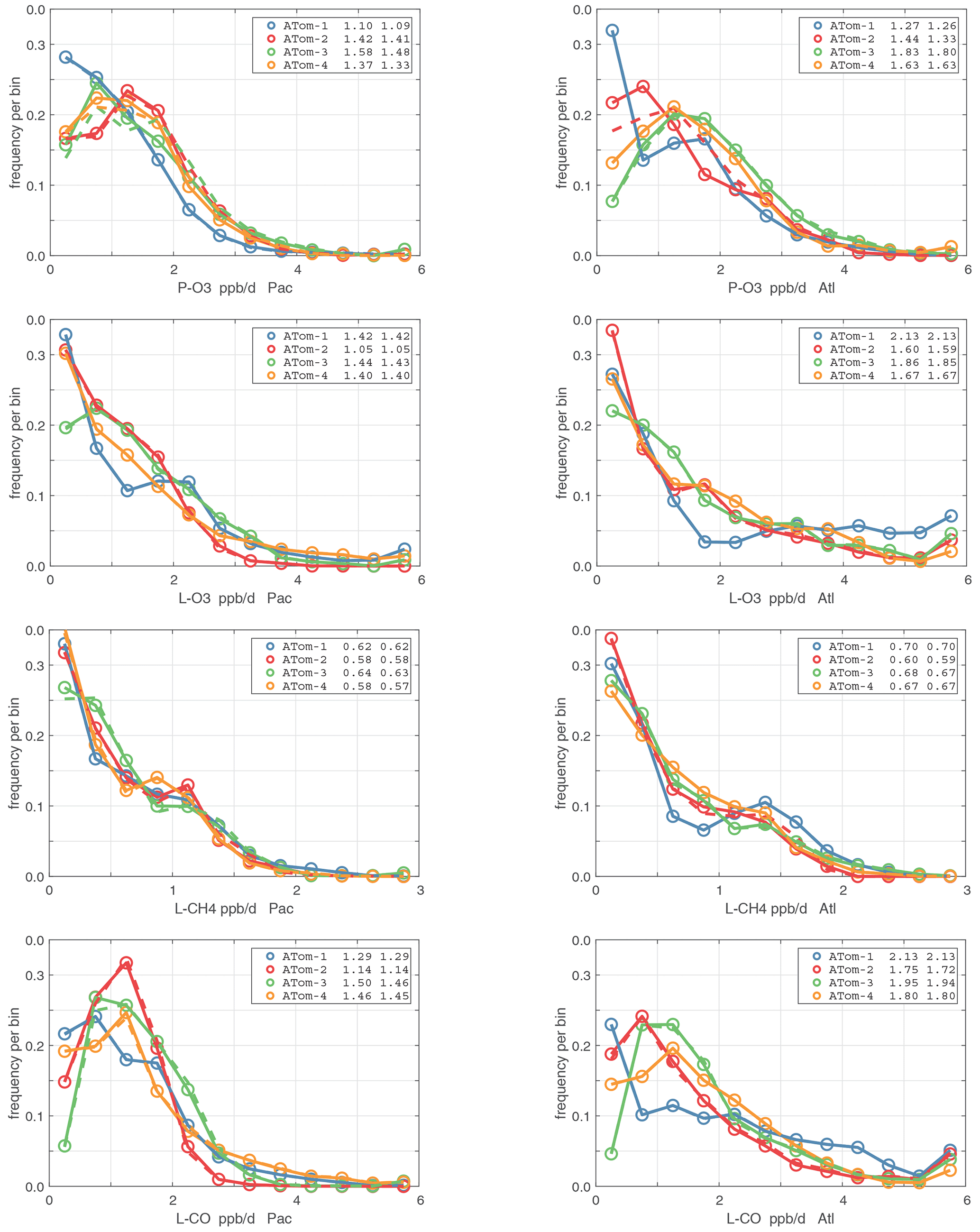
Figure 55 Probability density of the four reactivities (P-O3, L-O3, L-CH4, L-CO; ppb d⁻¹) in (left) Pacific and (right) Atlantic basins.

For the Atlantic basins (53^∘ S–60^∘ N), all four ATom deployments are shown in each panel. Only the first day of each deployment is shown (and hence these are not identical to Figs. 40–43). Values in the legend are the basin-wide averages for each deployment, given as v2b (dashed lines) and then v3 (solid lines). See Fig. 40.

5.3 Distribution of the key ATom species

We examine the distribution of key species over the Pacific Ocean and Atlantic Ocean basins with mean profiles of NO_x (v2b), NOx^fit (v3), and HOOH in Fig. 56. In the Pacific, the impact of v3 NO_x (labeled NOxx) is to reduce some high values in ATom-34 and make ATom-234 almost identical in the Pacific. ATom-1 NO_x remains much smaller than the other deployments. In the Atlantic, the v2b–v3 changes are not obvious, except for reducing the ATom-2 values below 3 km to look more like ATom-1. HOOH profiles often show a peak (500–1000 ppt) in the lower troposphere, 1–5 km, with the Atlantic usually being larger. For Pacific ATom-1, NO_x (and P-O3) is particularly low, but HOOH (and L-O3) is particularly high.

Given the importance of the tropics, we replot these profiles of NO_x(v2b), NOx^fit(v3), and HOOH for the three tropical regions in Fig. 57. The central Pacific is not much affected by the v2b–v3 update, but the eastern Pacific and tropical Atlantic noticeably change. For Pacific HOOH, we find that the 1–5 km peak is mostly in the eastern Pacific and thus relate high levels of HOOH and related HO_x activity to outflow from continents.

The 2D curtain files for the Pacific and Atlantic basins show the level of heterogeneity in NO_x for ATom-1234 in Figs. 58–59. These two figures compare NO_x (v2b) with NO_x (v3) in the Pacific and Atlantic, respectively. The biggest changes from v2b to v3 in the Pacific occur for ATom-34 and are due to the eastern Pacific flights as noted earlier. In these plots the eastern Pacific profiles overlap with the central Pacific profiles, and so some heterogeneity in this region is caused by longitudinally distant, not-along-flight parcels. Similarly, for ATom-234, the North Pacific curtain plots here include two separate flights: one in the eastern Pacific from Palmdale to Anchorage and, a few days later, one in the central Pacific from Anchorage to Kona. Overall, the NO_x shows that high values (> 100 ppt) consistently but sporadically occur at the uppermost flight levels. These high-NO_x parcels are probably due to lightning from deep convection, predominantly over continents, and they are the cause of high P-O3 values in the 10–12 km region of most ATom flights.

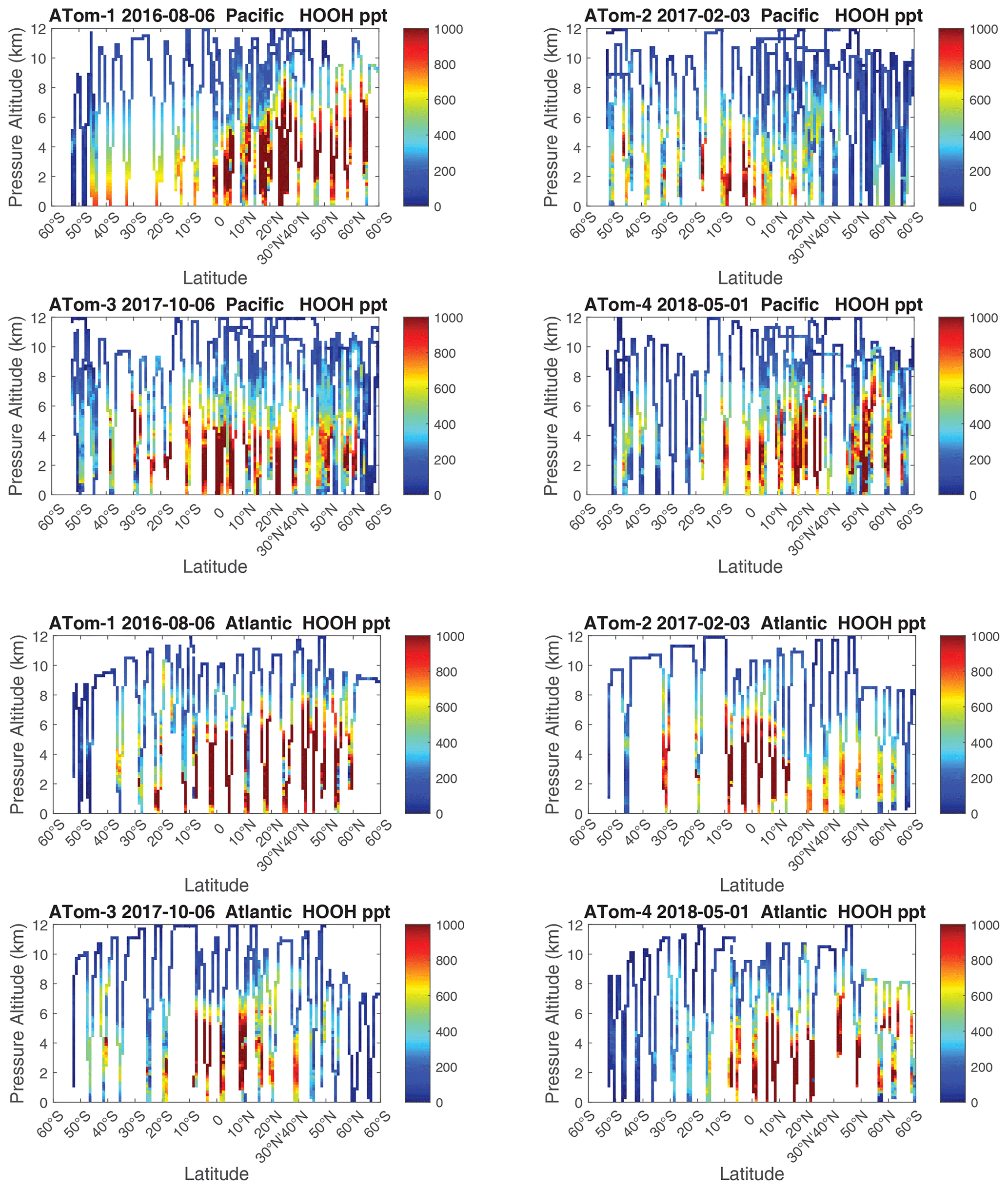
Figure 60 shows HOOH for both basins (eight panels). Unlike NO_x, the HOOH patterns show extensive regions, 30^∘ in latitude or wider, mostly tropical, with abundances > 1000 ppt between 1 and 6 km. This pattern is expected with a large, somewhat homogeneous chemical source of HOOH that partly follows the sun with each ATom deployment. We often find that the high-NO_x regions are separated from the high-HOOH ones. An unusual block of mid-tropospheric air was sampled in the South Pacific (30–15^∘ S) during ATom-3 (Fig. 58). This air mass had uniformly high NO_x values (60–100+ ppt) not typical of convective high-altitude NO_x. These NO_x values were directly measured and are not affected by the v2b–v3 shift. The anticorrelation with HOOH (Fig. 60) is surprising: high levels of HOOH surround the separate high-NO_x air mass. Given the overall importance of high-NO_x and (separately) high-HOOH regions to the chemical budgets, it would be valuable to check the CTM and CCM modeling of this feature to understand its cause.

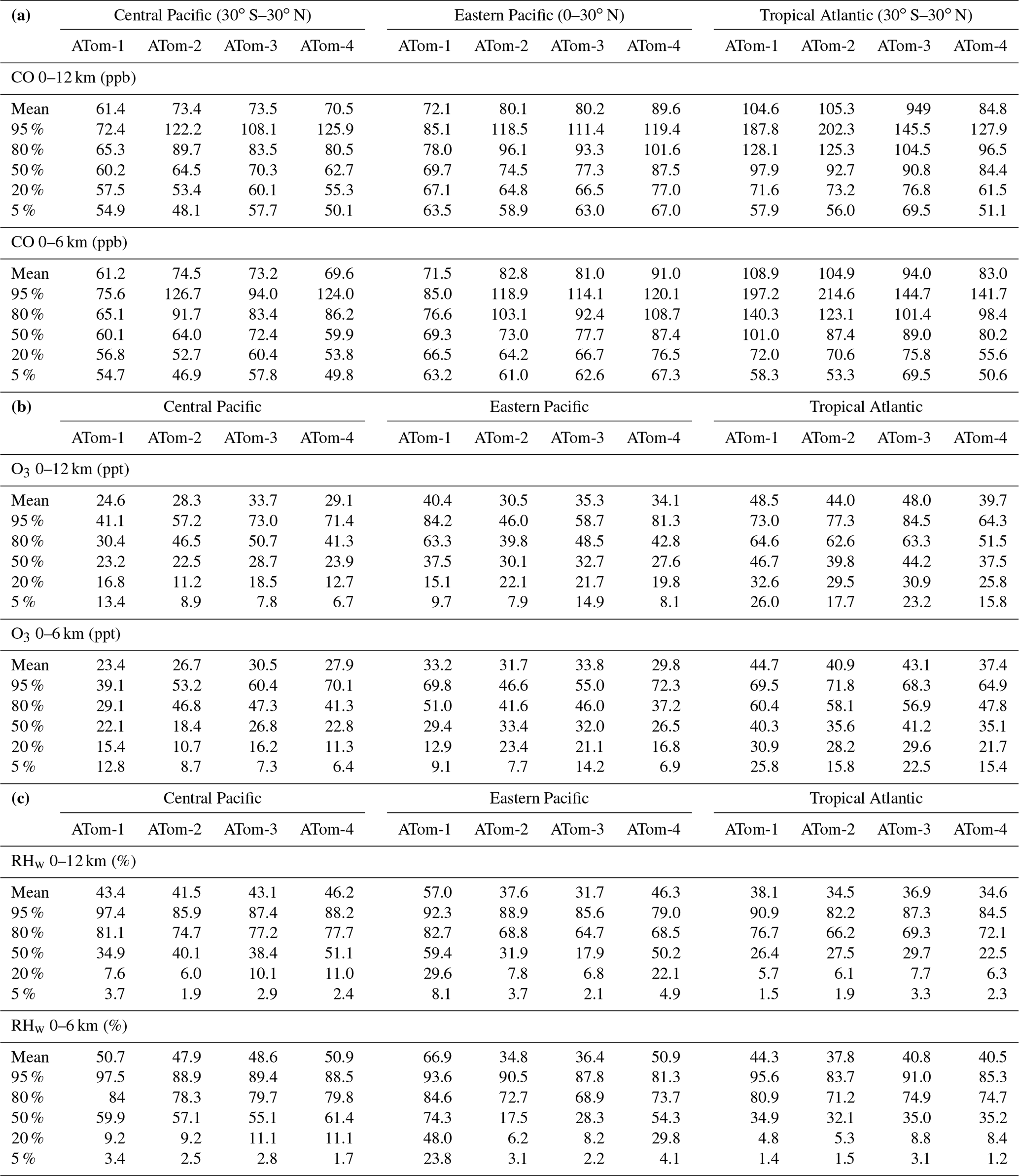
Figures 61–64 show the PDs of CO (ppb), O₃ (ppb), relative humidity over water (RH_w, %), and NO_x (log(ppt)) for the tropical ocean regions (central Pacific, eastern Pacific, tropical Atlantic). The PDs are calculated for the lower troposphere (0–6 km) and the full ATom-sampled troposphere (0–12 km). For the first three quantities, the legend for each deployment lists the mean value, standard deviation, and skewness, while for NO_x, whose PD uses log([NO_x]), the legend lists just the mean value (ppt) and the mean log value (converted back to parts per trillion).

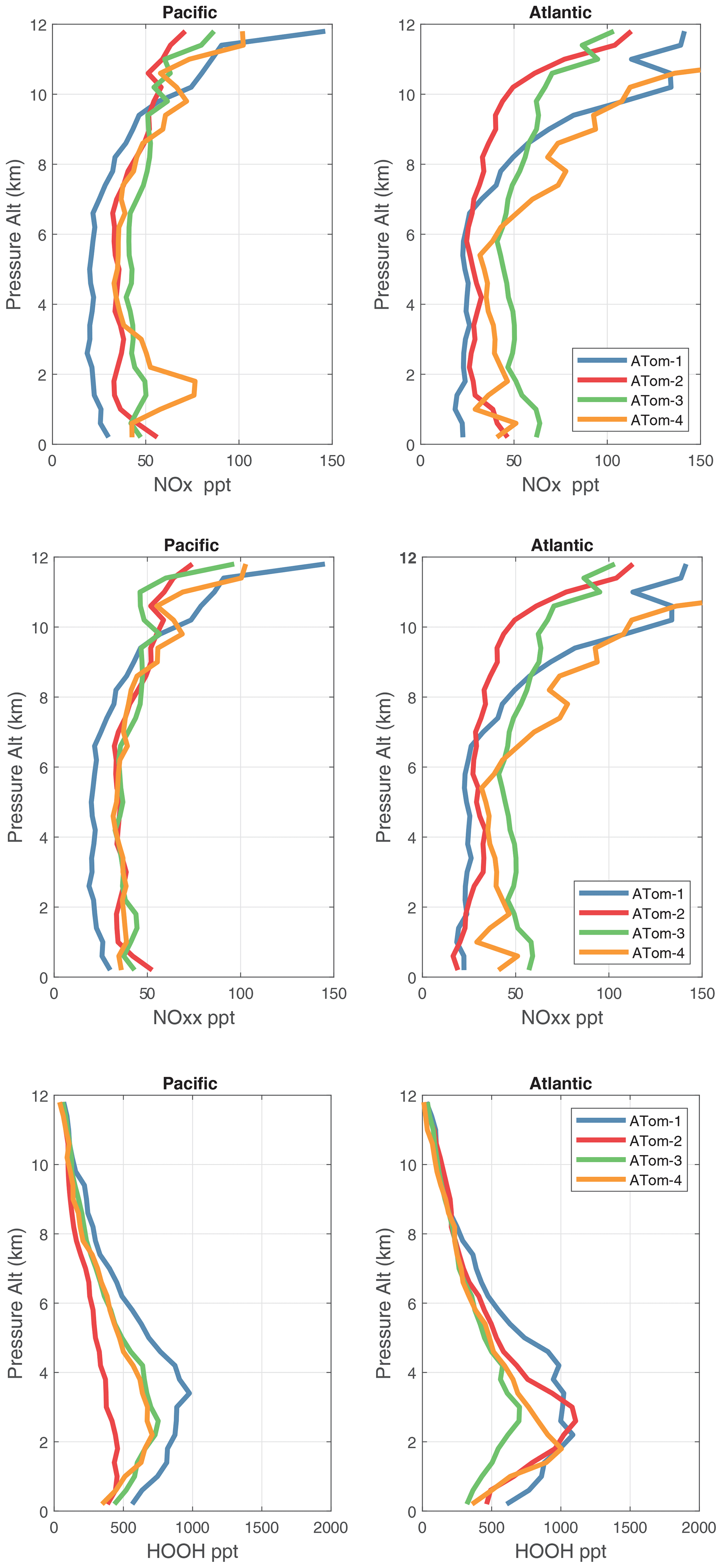
Figure 56 Vertical mean profiles (parts per trillion vs. pressure altitude) of NO_x (v2b), NOxx (NO_x v3), and HOOH over the Pacific and Atlantic basins. Standard weighting (see text).

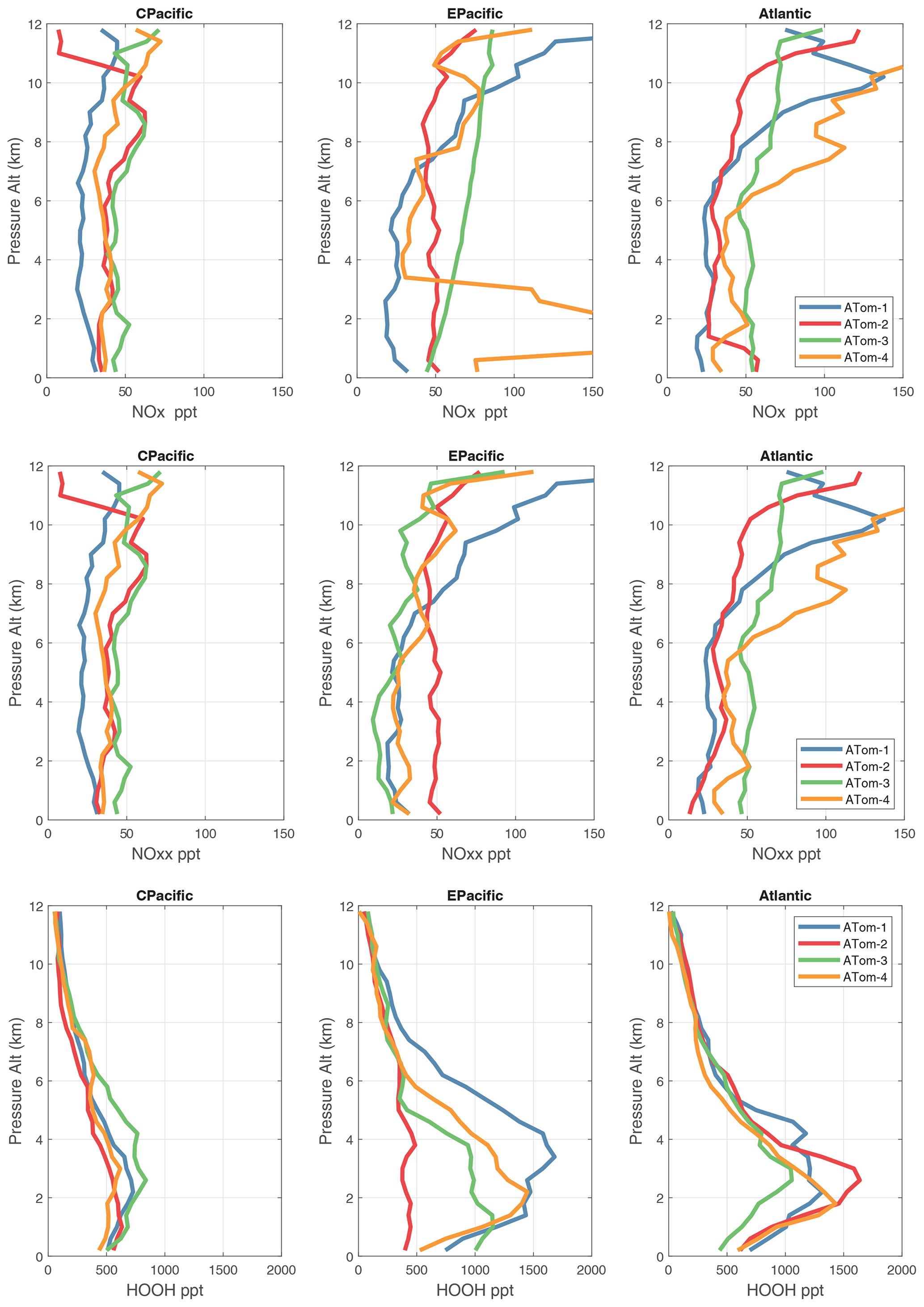
Figure 57 Vertical mean profiles (parts per trillion vs. pressure altitude) of NO_x (v2b), NOxx (NO_x v3), and HOOH (v2b) over the three tropical ocean regions (central Pacific, eastern Pacific, and Atlantic). See Fig. 56.

G2023 in their Fig. 4 compared the ATom-1 PDs for NO_x, HCHO, and HOOH with six CTM and CCM climatologies for August and showed some clearly divergent model results. We believe that these ATom PDs provide a valuable model metric and can be used to track down model errors. Here we compare the ATom-1234 PDs for CO, O₃, RH_w, and NO_x because these are critical species based on the sensitivities (Table 2). The NO_x PDs are paired with v3 vs. v2b panels: they show large shifts in the eastern Pacific, as expected from earlier comparisons. The tropical Atlantic NO_x PDs also show large shifts with the versions. Thus, the NO_x PDs should be used with caution, although the central Pacific PDs look similar across the four deployments and should provide a robust statistic on the NO_x distributions in the 0–12 km altitude range. For CO, O₃, and RH_w, we find that the central Pacific and tropical Atlantic PDs are stable across deployments and should present an excellent observational climatology metric for the models. The eastern Pacific PDs vary greatly with deployment and do not represent a stable climatology.

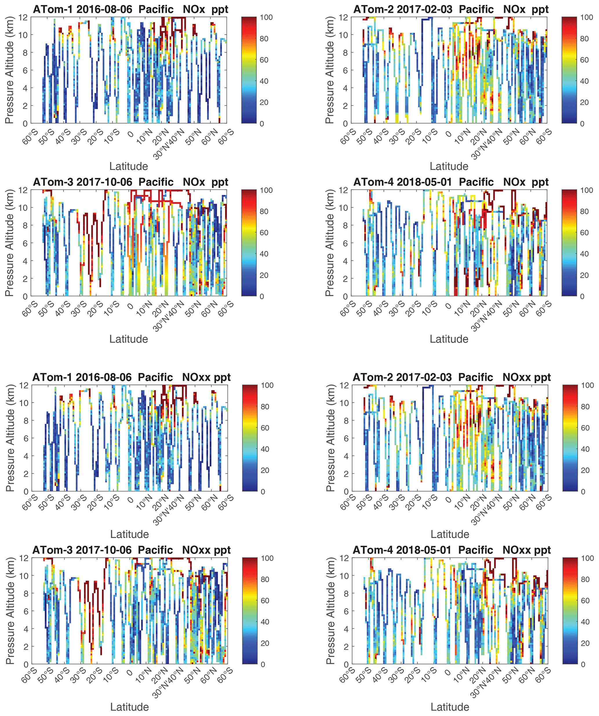
Figure 58 Two-dimensional Pacific curtain profiles for ATom-1234 of NO_x (v2b) and NOxx (NO_x v3).

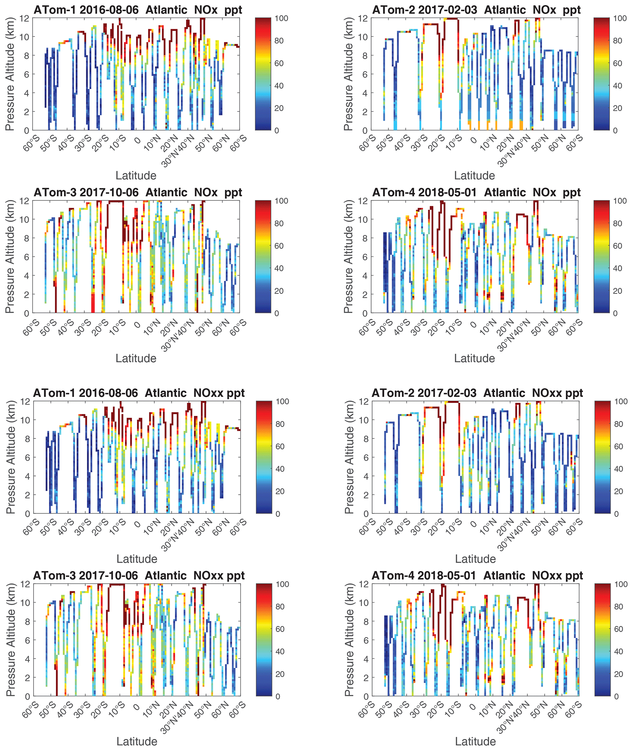
Figure 59 Two-dimensional Atlantic curtain profiles for ATom-1234 of NO_x (v2b) and NOxx (NO_x v3).

Figure 60 Two-dimensional Pacific and Atlantic curtain profiles for ATom-1234 of HOOH.

The RH_w PDs are quite different from the chemical species. RH_w has a bimodal distribution for the tropical regions with a narrow peak probability below 10 % RH_w and a broad maximum of about 80 % RH_w. Thus, RH_w clearly distinguishes between two types of tropical air masses reflecting the Hadley cell: a humid, generally upwelling tropical air mass and a dry descending subtropical air mass. As for other species and reactivities, the eastern Pacific RH_w is highly variable with deployment, showing that ATom-14 (the more reactive periods) lacks dry air with RH_w < 20 %, consistent with the sensitivity to H₂O and the high reactivities noted above. For convenience in model comparisons, a tabulated version of the CO, O₃, and RH_w PDs, giving values for the 5th, 20th, 50th, 80th, and 95th percentiles for each basin and deployment, is provided in Table 5.

The use of two-dimensional PDs for species as a way of comparing models and measurements was investigated previously (P2017, P2018, and Fig. 7 of G2023). We do not pursue examples here but recommend that these 2D PDs of critical species defined from the sensitivity analyses, including the fitted ellipses, be tested as model metrics.

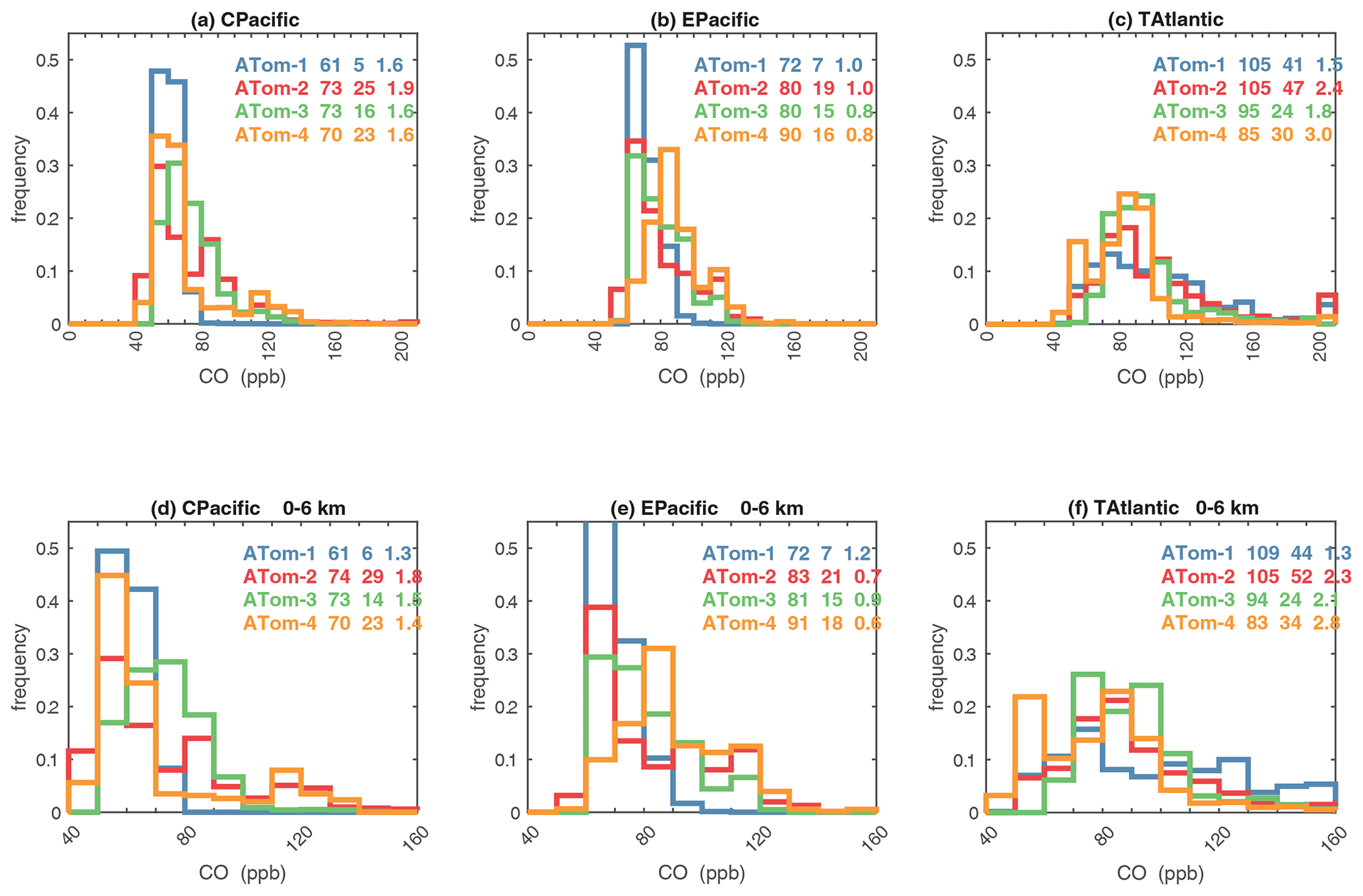
Figure 61 Probability density of CO (ppb) in the three tropical basins (30^∘ S–30^∘ N) for ATom-1234. The standard weighting of ATom 10 s air parcels is used. The lower panel shows the 0–6 km pressure altitude where most of the chemical reactivity is located, while the upper panel shows the full troposphere, approximately 0–12 km. The color coding in the legend identifies the four ATom deployments. The numbers in the legend are, successively, the mean value, standard deviation, and skewness in parts per billion.

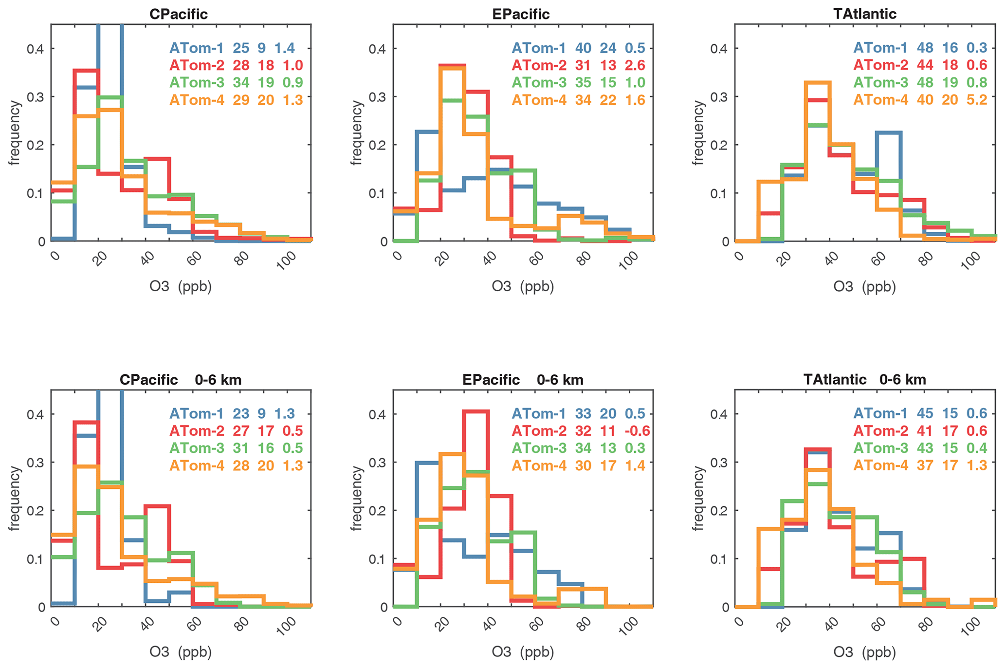
Figure 62 Probability density of O₃ (ppb) in the three tropical basins (30^∘ S–30^∘ N) for ATom-1234. See Fig. 61. The numbers in the legend are, successively, the mean value, standard deviation, and skewness in parts per billion.

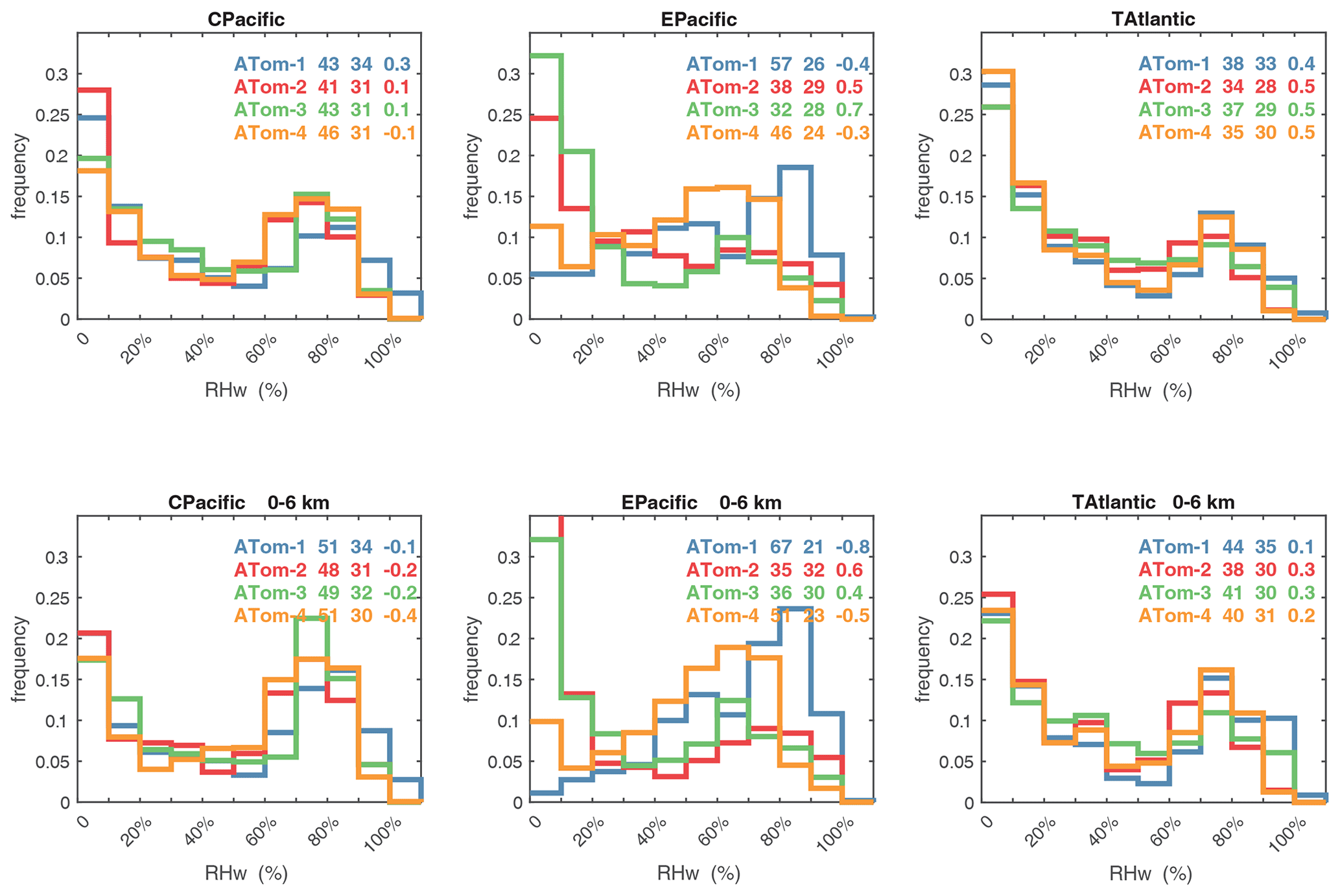
Figure 63 Probability density of the relative humidity over liquid water (RH_w, %) in the three tropical basins (30^∘ S–30^∘ N) for ATom-1234. See Fig. 61. The numbers in the legend are, successively, the mean value, standard deviation, and skewness in percentage.

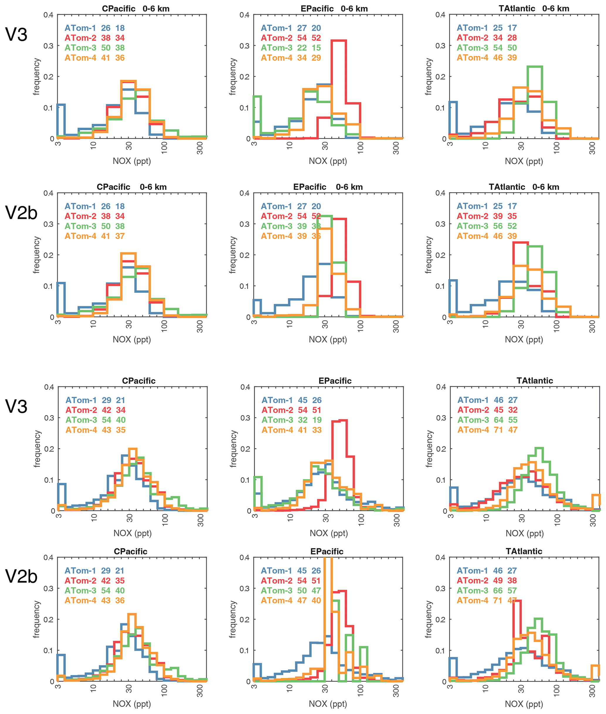
Figure 64 Probability density of log₁₀(NO_x, ppt) in the three tropical basins (30^∘ S–30^∘ N) for ATom-1234, comparing MDS versions 3 and 2b. See Fig. 61. The numbers in the legend are, successively, the mean value of NO_x and the mean value of log₁₀(NO_x), both in parts per trillion. The four successive rows are 0–6 km for MDS V3 and V2b and 0–12 km for MDS V3 and V2b.

Table 5 Probability densities of three key quantities for the tropical oceans: (a) CO (ppb), (b) O₃ (ppb), and (c) RHw (%).

5.4 Heterogeneous chemistry

The potential role of heterogeneous (gas–aerosol) chemical reactions – which are not included in this study – is illustrated with the profiles of aerosol surface area density (SAD) (µm² cm⁻³) in Fig. 65. We calculate SAD as the sum of the four reported modes (nucleation, Aitken, accumulation, and coarse), with most of the area coming from the accumulation and coarse modes. In the Pacific, above the marine boundary layer, SAD is usually < 20 µm² cm⁻³), while in the Atlantic SAD is much larger, 20–80 µm² cm⁻³, everywhere below 4 km. This difference is extensive in all seasons and is clearly due to low-altitude continental convection from, e.g., biomass burning. There is one example in these profiles where such convection delivers high aerosol loading near 6 km in the eastern Pacific (ATom-4). We calculate the frequency distribution of reactions for all the parcels in ATom-1 Pacific and Atlantic assuming a high-reactivity coefficient gamma = 0.10 in Fig. 66. If we are looking for heterogeneous reactions to compete with radical chemistry rates (e.g., ROO, HO₂), then we need a high gamma and reaction frequency > 2 h⁻¹. For ATom-1 Pacific, this occurs in only 3 % of the parcels, while for ATom-1 Atlantic, it is 17 % of the parcels (as seen by the large SAD below 4 km). This evidence indicates that heterogeneous chemical reactions are likely not important in the reactivity statistics here, but a more thorough analysis considering the aerosol composition and realistic gammas is needed.

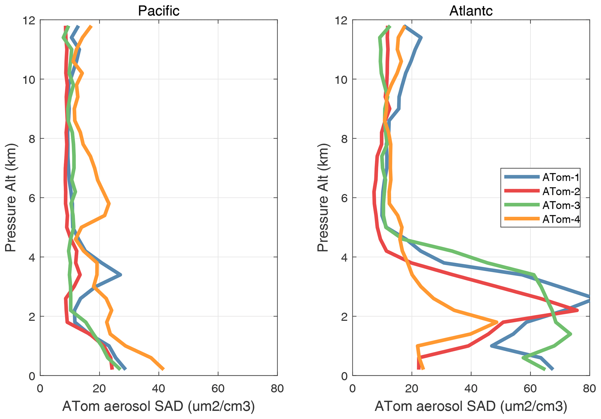
Figure 65 Vertical mean profiles of aerosol surface area density (SAD, µm² cm⁻³) over the Pacific and Atlantic basins. Standard weighting (see text). SAD is the sum of the four reported modes (nucleation, Aitken, accumulation, and coarse), with most of the area from the accumulation and coarse modes.

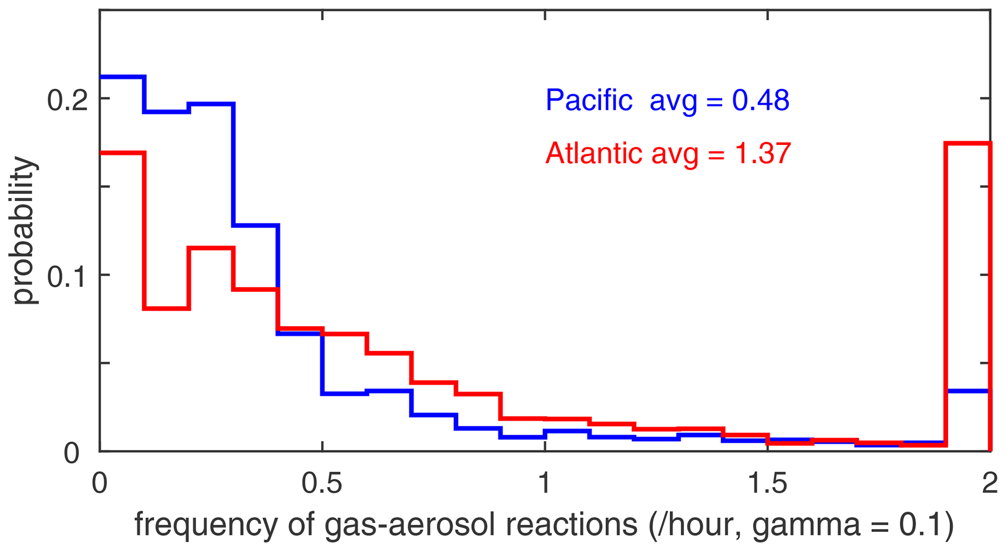
Figure 66 Frequency distribution of gas–aerosol reactions (per hour) for ATom-1 Pacific (blue) and Atom-1 Atlantic (red) assuming a high-reactivity coefficient gamma equal to 0.10.

6 Chemical feedbacks

6.1 Timescale for O₃ perturbations

The sensitivities calculated for the parcels in ATom-1 allow us to estimate the timescale for an O₃ perturbation. Most modeling studies make the simplistic assumption that the P-O3 and L-O3 derived from the rates defined above are the key terms in the continuity equation and, further, that P-O3 is constant, while L-O3 is linear in [O₃].

$$\begin{array}{}\text{(3)}& \begin{array}{rl}{\displaystyle \frac{\mathrm{d}\left[{\mathrm{O}}_{\mathrm{3}}\right]}{\mathrm{d}t}}& =\mathrm{PO}\mathrm{3}-\mathrm{LO}\mathrm{3}=P^{\text{constant}}\\ & -\left[{\mathrm{O}}_{\mathrm{3}}\right]\left\{{\displaystyle \frac{\text{L-O3}}{\left[{\mathrm{O}}_{\mathrm{3}}\right]}}\right\}=P^{\mathrm{constant}}-{\displaystyle \frac{\left[{\mathrm{O}}_{\mathrm{3}}\right]}{T^{\mathrm{A}}}}\end{array}\end{array}$$

The approximate timescale, T^A= [O₃]$/$L-O3, is often called the O₃ lifetime because the steady-state concentration is proportional to it: [O₃]^steady-state=P^constantT^A. This approximation is valid only if

$$\begin{array}{}\text{(4)}& {\displaystyle \frac{\mathrm{dln}\left[\text{L-O3}\right]}{\mathrm{dln}\left[{\mathrm{O}}_{\mathrm{3}}\right]}}\equiv \mathrm{1}\mathrm{and}{\displaystyle \frac{\mathrm{dln}\left[\text{P-O3}\right]}{\mathrm{dln}\left[{\mathrm{O}}_{\mathrm{3}}\right]}}\equiv \mathrm{0},\end{array}$$

but instead, from Table 4, for ATom-1 Atlantic we have

$$\begin{array}{}\text{(5)}& {\displaystyle \frac{\text{dln}\left[\text{L-O3}\right]}{\mathrm{dln}\left[{\mathrm{O}}_{\mathrm{3}}\right]}}\equiv \mathrm{1.01}\mathrm{and}{\displaystyle \frac{\mathrm{dln}\left[\text{P-O3}\right]}{\mathrm{dln}\left[{\mathrm{O}}_{\mathrm{3}}\right]}}\equiv -\mathrm{0.41}.\end{array}$$

So, L-O3 is very close to linear in [O₃], but P-O3 decreases as [O₃] increases, and thus the net P minus L (Eq. 3) decreases more quickly, and an [O₃] increase decays more quickly than given by T^A. The true timescale T^T is given by the linearized O₃ loss frequency.

$$\begin{array}{}\text{(6)}& {\displaystyle \frac{\mathrm{1}}{T^{\mathrm{T}}}}={\displaystyle \frac{\mathrm{d}\left[-\frac{{\mathrm{dO}}_{\mathrm{3}}}{\mathrm{d}t}\right]}{\mathrm{d}\left[{\mathrm{O}}_{\mathrm{3}}\right]}}\approx {\displaystyle \frac{\mathrm{d}\left[\text{L-O3}-\text{P-O3}\right]}{\mathrm{d}\left[{\mathrm{O}}_{\mathrm{3}}\right]}}\end{array}$$

Figure 67 shows this linearized O₃ loss frequency ($\mathrm{1}/T^{\mathrm{T}}$, units of per day) for the Pacific and Atlantic flight profiles of ATom-1. High values > 0.15 d⁻¹ occur throughout the northern tropics below 5 km. In the upper troposphere, the timescale for O₃ is slow, 20 d or longer. Basin-mean loss frequency is similar in both the Pacific (0.065 d⁻¹) and Atlantic (0.061 d⁻¹), corresponding to a mean timescale T^T ∼ 16 d.

Profiles of the mean loss frequency, both $\mathrm{1}/T^{\mathrm{T}}$ and $\mathrm{1}/T^{\mathrm{A}}$, are shown for the Pacific and Atlantic basins in Fig. 68. Both basins show almost the same profiles, increasing from 0.01 d⁻¹ at 12 km to ∼ 0.1 d⁻¹ near the surface, with near-constant differences, $\mathrm{1}/T^{\mathrm{T}}$–$\mathrm{1}/T^{\mathrm{A}}$, of about +0.01 d⁻¹. Thus, the relative error in T^A decreases from 100 % at 12 km to 10 % at 0 km. The profiles of P-O3 and L-O3 in the basins in Fig. 68 indicate the shifting importance of the d[P-O3]$/$d[O₃] term with altitude.

Our sensitivity calculations are made with 24 h integrations, and over this time the HO_x and NO_x radicals readjust to the O₃ increase, other species like HOOH partially respond, and for longer-lived key species such as CO (90 d) the adjustment is negligible. For O₃, the timescales for decay of the perturbation are 10–30 d, and thus we can ignore to first order any feedbacks on the chemistry caused by changes in CO or C₂H₆ or CH₄. Other longer-chain alkanes might readjust in 10–30 d to the new levels of O₃, but these species are not very important for the ATom oceanic flights. Thus, our 24 h sensitivity calculations should be adequate for deriving the timescale for decay of an O₃ perturbation.

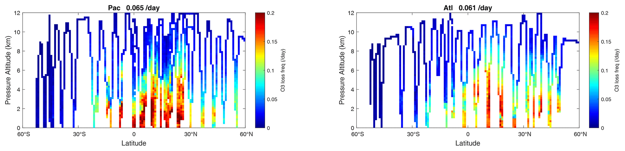
Figure 67 Two-dimensional curtain plots of the linearized loss frequency for O₃ ($\mathrm{1}/T^{\mathrm{T}}$ in units of per day) for the ATom-1 Pacific and Atlantic basins. The loss frequency is calculated from the sensitivity calculation dln(L-O3 minus P-O3)$/$dln(O₃).

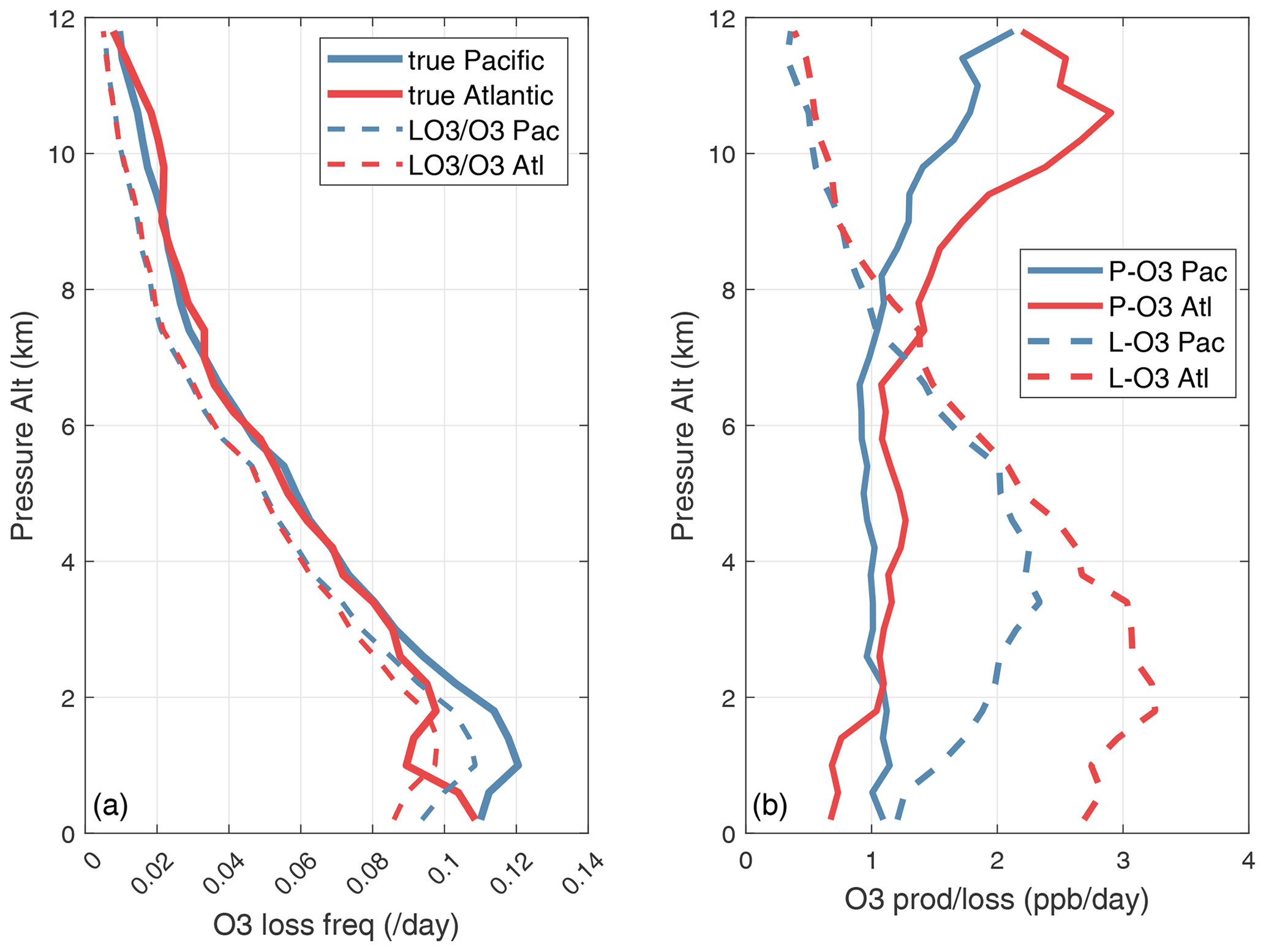
Figure 68 (a) O₃ loss frequency (d⁻¹) vs. pressure altitude (km), averaged over the Pacific (blue) and Atlantic (red) basins for ATom-1. The true linearized loss frequency ($\mathrm{1}/T^{\mathrm{T}}$, solid lines) is compared with the often-used approximation ($\mathrm{1}/T^{\mathrm{A}}=$ L-O3$/$O₃, dashed lines). (b) Altitude profiles for both ocean basins of P-O3 (solid) and L-O3 (dashed), both in parts per billion per day.

6.2 CH₄ lifetime feedback

A positive perturbation to the CH₄ abundance reduces tropospheric OH and thus increases the timescale of the perturbation relative to its steady-state lifetime (Prather, 1994, 1996). A measure of this chemical feedback is the sensitivity calculated here, dln[L-CH4]$/$dln[CH4] (percentage per percentage). These sensitivities, for all ATom-1 10 s parcels including continental data, are plotted vs. L-CH4 as small black dots in Fig. 69. The basin-mean values are shown for the Pacific (large red dot, 0.76 % per percentage) and the Atlantic (large blue dot, 0.80 % per percentage). The number we want from these calculations is the sensitivity of the OH weighted by the CH₄ loss (i.e., including the temperature factor in the rate coefficient, exp(−1775$/T$)).

$$\begin{array}{}\text{(7)}& s_{\mathrm{OH}}={\displaystyle \frac{\mathrm{dln}\left[\text{L-CH4}\right]}{\mathrm{dln}\left[{\mathrm{CH}}_{\mathrm{4}}\right]}}-\mathrm{1}\end{array}$$

The values of s_OH for the ATom-1 parcels are plotted for the Pacific and Atlantic flight profiles in Fig. 70a and b, and the mean values are −0.24 and −0.20, respectively. The value of s_OH is the most negative, about −0.3 in the lower troposphere, where CH₄ dominates the chemistry and controls much of the OH loss. The value of s_OH drops to below −0.1 in the upper troposphere, where cold temperatures make the OH + CH₄ reaction very slow compared with the OH + CO reaction. The CH₄ feedback factor describes the increase in the timescale for a CH₄ perturbation relative to the OH lifetime in steady state (i.e., the OH lifetime is the atmospheric burden divided by loss to OH reactions).

$$\begin{array}{}\text{(8)}& {\mathrm{ff}}_{{\mathrm{CH}}_{\mathrm{4}}}={\displaystyle \frac{\mathrm{1}}{\mathrm{1}+s_{\mathrm{OH}}}}\end{array}$$

The values of ff${}_{{\mathrm{CH}}_{\mathrm{4}}}$ along the flights tracks vary from about 1.2 to 1.6: see Fig. 70c and d. Averaging the two basins for s_OH, we calculate a mean ff${}_{{\mathrm{CH}}_{\mathrm{4}}}\sim$ 1.28.

This 24 h calculation, however, does not include the adjustment to other key species that will occur in response to the decadal decay of a CH₄ perturbation. The correct way to model this is to run CTM and/or CCM perturbation + control sequences for several years with different CH₄ lower-boundary conditions (e.g., Holmes, 2018). During this time other species, specifically CO, which is the other major sink of OH radicals, will adjust to the CH₄-driven changes in OH. The CO change, an increase, will then further reduce OH and amplify the ff${}_{{\mathrm{CH}}_{\mathrm{4}}}$.

We can make a simple, first-order estimate of this CO adjustment to a 10 % CH₄ increase. The s_OH directly from the CH₄ change averages −0.22 (Table 2, average of the Pacific and Atlantic) or −2.2 % in the loss frequency of CH₄. The change in L-CO from the 10 % CH₄ increase is −1.9 % (Table 2, average of the Pacific and Atlantic). If CO is in balance between the sources and L-CO, then CO will increase by 1.9 %. The two-basin average sensitivity of L-CH4 to CO is −0.37, so the CO increase will decrease L-CH4 by a further −0.7 % to −2.9 %. The updated $s_{\mathrm{OH}}^{*}$ is −0.29, a 30 % increase in magnitude, and the ff${}_{{\mathrm{CH}}_{\mathrm{4}}}^{*}$ is 1.41. This CO amplification may be an overestimate as some of the CO sources, from CH₄ specifically, will be reduced with OH. Another correction is that the feedback factor used to calculate the perturbation time for a CH₄ pulse must be derived from the total CH₄ lifetime that includes losses in the stratosphere and from soils where the loss frequencies do not respond to a CH₄ perturbation (e.g., Holmes, 2018). This full budget calculation gives a reduced s_TOTAL of −0.25 and ff = 1.34, quite in line with recent global model results (1.30 ± 0.07, Thornhill et al., 2021b). We do not support the use of ATom-like chemical climatologies as a comparable result relative to the CTM or CCMs, but they do provide a measurement check point and estimate of first-order responses of tropospheric chemistry to global change.

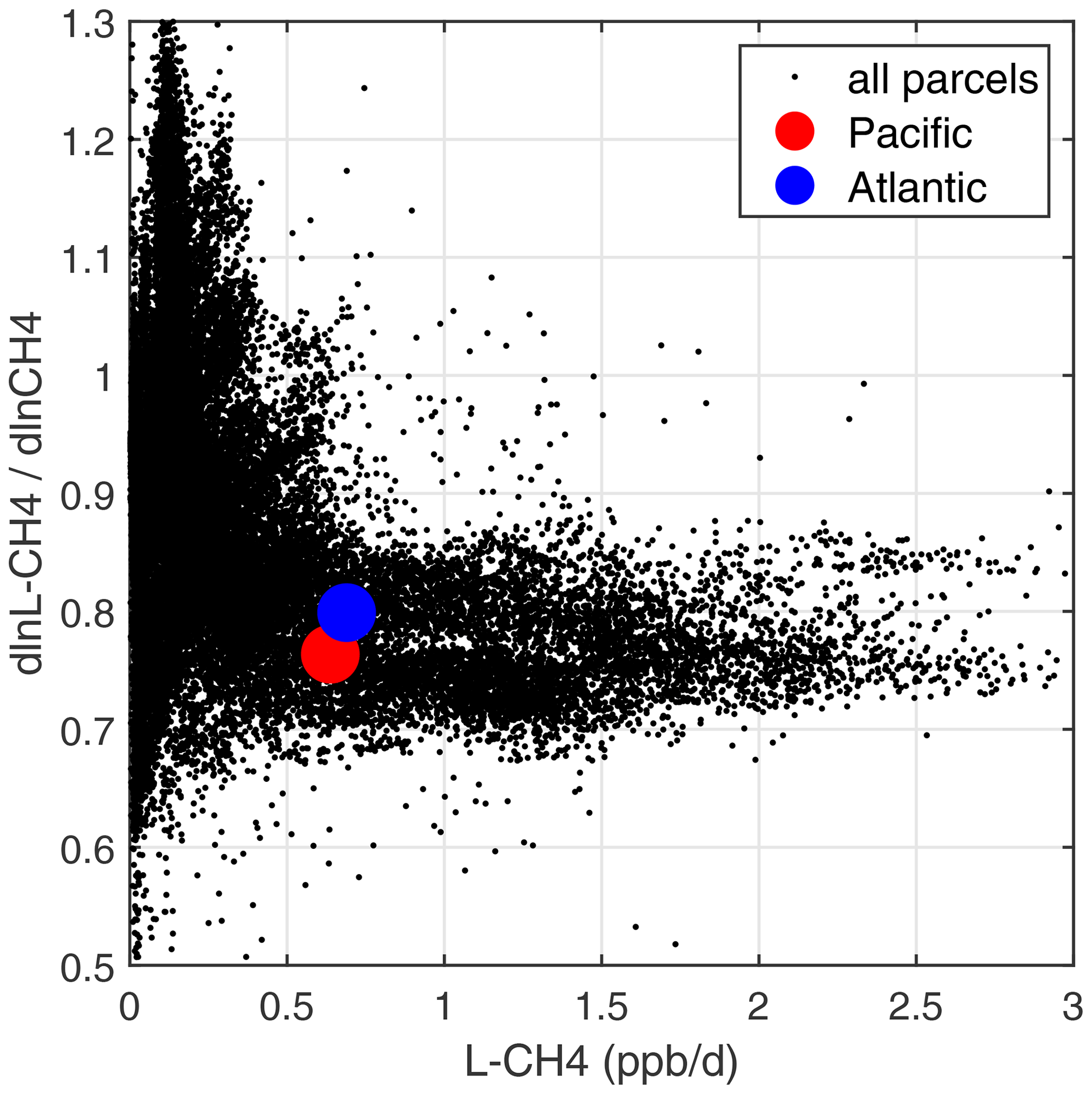
Figure 69 Sensitivity of CH₄ loss with respect to its abundance (dln[L-CH4]$/$dln[CH₄], in percentage per percentage) vs. loss rate (L-CH4, in parts per billion per day) for parcels in ATom-1. All ATom-1 10 s parcels, including continental data, are plotted (small black dots) together with the basin-mean values for the Pacific (red dot) and Atlantic (blue dot).

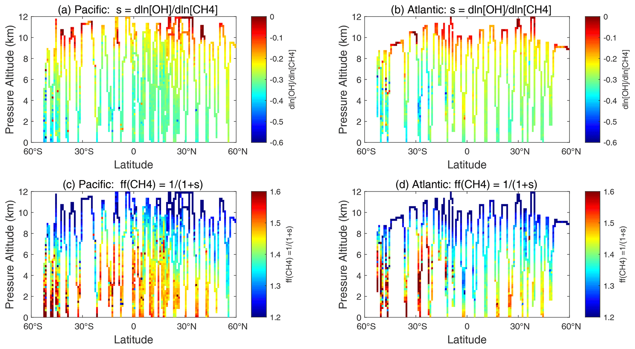
Figure 70 Two-dimensional curtain plots from ATom-1 of (a, b) the OH sensitivity to CH₄, s_OH= dln[OH]$/$dln[CH₄] = dln[L-CH4]/dln[CH₄] −1, for the Pacific and Atlantic basins, and (c, d) the CH₄ lifetime feedback factor ff${}_{{\mathrm{CH}}_{\mathrm{4}}}=\mathrm{1}/(\mathrm{1}+s_{\mathrm{OH}})$ for the same.

7 Code and data availability

The full raw ATom data set was first posted short-term on the NASA ESPO ATom website (https://espo.nasa.gov/atom/content/ATom, NASA ESPO, 2023). The final archive for the ATom data and merged data sets will be at Oak Ridge National Laboratory (ORNL) (see https://daac.ornl.gov/ATOM/guides/ATom_merge.html, Wofsy et al., 2021). The MDS and RDS data sets together with the MATLAB codes and some intermediate data used in this analysis are posted on Dryad (https://doi.org/10.7280/D1B12H; see Prather et al., 2023). Earlier versions, primarily for ATom-1 based on Guo et al. (2021, 2023), are posted on Dryad (https://doi.org/10.7280/D1Q699; see Guo, 2022a, and the link to https://doi.org/10.5281/zenodo.5905661 in Guo, 2022b).

8 Conclusions and perspective

This paper completes the presentation and analysis of the ATom observations focusing on reactive, gas-phase chemistry affecting the tropospheric budgets of CH₄ and O₃. For the four seasonal deployments of ATom-1234 (August, February, October, and May, respectively), we use the profiling curtains to identify large-scale regions of the troposphere that drive the budgets, particularly in the lower troposphere for loss of O₃ and CH₄ as well as the smaller heterogeneities, particularly in the upper troposphere for NO_x-driven hotspots of O₃ production. These results are the first near-global views of the remote troposphere, primarily the middle of the Pacific Ocean and Atlantic Ocean basins, from the perspective of their net chemical reactivities based on observations at 200 m scales. Statistics are also accumulated for the Southern Ocean and the Arctic basin but, as expected from global chemistry models, these regions contribute little to the global O₃ and CH₄ budgets.

ATom's regular profiling of the ocean basins allows for weighted averages to build probability densities for key species and reactivities. Although the individual curtain plots for each ocean transect show clear meteorological variability for each deployment, these probability densities are quite similar and provide a robust test for the modeled distribution of species and reaction rates. For example, the 30^∘ S–30^∘ N tropical distributions of O₃, CO, and relative humidity are distinct between the Pacific and Atlantic (higher values of both) but similar for each deployment in each basin. On the other hand, the eastern Pacific transect (0–30^∘ N, 121^∘ W) is very different for each deployment. The compelling statistics built up from the ATom deployments are a metric that should be used to evaluate our current global chemistry models.

The Modeling Data Stream (MDS) developed for ATom (G2023 plus this publication) relies on gap-filling for sporadic measurements or missing data and is essential if reactivities for the 10 s air parcels are to be calculated without losing most of the parcels. The MDS concept was a reasonable and necessary step for the Reactivity Data Stream (RDS); however, as we have seen with the successive MDS versions, there is a painful learning curve for what to do with missing data, and no truly optimal method has been identified yet. The MDS and RDS approach defined in the pre-ATom deployment papers (P2017 and P2018) is still the best method for calculation of diel-averaged rates. The ATom method of inserting the observed chemical composition of 10 s parcels into global chemistry models to calculate reaction rates (RDS) remains a compromise: integrating without sources or sinks means that NO_x and alkanes decrease over 24 h, while HOOH and CH₃OOH increase. We cannot identify a method of including these that does not also prejudice the results and that remains easy to implement in most global models. One improvement might be to use satellite-derived photolysis rates for the day of observation (e.g., Holmes, 2016) rather than just having the models pick 5 d from their own meteorology fields to average over.

The calculation of reactivities (R) with the RDS protocol allows us to go further and derive the sensitivity factors (S= dln(R)/dln(X)) relative to the chemical species (X). From these sensitivities, we can identify the critical species where model error in their atmospheric simulation will cause large errors in the budgets. This information is useful in directing model–measurement comparisons. From the sensitivities, we have also derived correctly linearized lifetimes and even the CH₄ chemical feedback. Admittedly these are only first-order estimates and do not include the full set of feedbacks in a flux-driven, free-running global chemistry model. Nevertheless, it does provide an independent estimate based primarily on observations.

The ATom measurements can make a substantial contribution to understanding model differences and even identifying model errors in global tropospheric chemistry. What is clear from this measurement–model analysis since P2017 is that most of the model difference is caused by models calculating different climatologies for the key species such as O₃, CO, H₂O, NO_x, CH₄, and T. When models use the same distribution of key species, they calculate nearly the same reactivities even though their chemical models have a wide range of species and complexities.

There remain uncertainties in kinetic rates and cross sections, yet models tend to use the same values (e.g., Burkholder et al., 2020). Using a fixed MDS chemical composition, the model differences are due mostly to variability in photolysis rates driven by clouds (Hall et al., 2018). For example, the model–model root-mean-square differences in reactivities adopting the same chemical composition are ∼ 10 % using the same model but different years (and hence different cloud fields): they are ∼ 20 % for different models that come close to matching one another, they reach 50 % if those models use different H₂O and T, and they exceed 100 % for some models that are known to be aberrant in other diagnostics. Thus, the most important model metric to develop from the ATom measurements would be standard probability densities of the key species in those regions where reactivities are largest: the lower tropics for loss of O₃ and CH₄, the upper tropics for production of O₃. These could include co-variation patterns (2D probability densities in G2023). Sensitivity analysis of the 24 h reactivities provides some core data that we feel should become a standard part of CCM evaluations and intercomparisons.

The other ATom information, which is important to understand for tropospheric chemistry but is not readily a metric, is the unusual large-scale air masses (20^∘ in latitude) of high reactivity that are clearly transient events most likely of continental origin: ATom-3 southern tropical Atlantic large masses of high NO_x and high P-O3 surrounded by high L-O3; ATom-14 eastern Pacific huge air masses of very high L-O3. Overall, the ATom data set based on 10 s (2 km) air parcels has allowed us to partially deconstruct the spatial scales and variability that define tropospheric chemistry from composition to reactivity.