TCOM-CFC11 and TCOM-CFC12: a gap-free, observationally constrained global dataset of stratospheric CFC-11 and CFC-12 profiles (v2.0)

Understanding the long-term trends of ozone-depleting substances (ODSs), particularly CFC-11 (CFCl₃) and CFC-12 (CF₂Cl₂), is essential for evaluating the effectiveness of the Montreal Protocol. However, reliably estimating these trends is complicated by the inherent sparse spatial and temporal coverage of high-quality stratospheric observations, such as those from the Atmospheric Chemistry Experiment–Fourier Transform Spectrometer (ACE-FTS). To address this limitation, we have developed an innovative machine learning methodology to combine the strengths of sparse ACE-FTS observations with the continuous output of the TOMCAT global chemical transport model (CTM).

We use XGBoost regression to constrain the TOMCAT tracers against co-located ACE-FTS measurements, thereby creating the TCOM (TOMCAT CTM and Occultation-Measurement-based) stratospheric profile datasets for CFC-11 and CFC-12. The resulting TCOM datasets described here (version 2.0) provide continuous, gap-free, global, daily vertical profiles from 2000 to 2024. A comprehensive evaluation confirms the method's effectiveness, showing the corrected TCOM data clustering significantly closer to the observations than the CTM and successfully rectifying systematic biases in the raw TOMCAT output, particularly the prominent high biases in the mid-to-high latitudes and low biases in the lower stratosphere. Furthermore, interpretable machine learning analysis reveals that the XGBoost model primarily functions here as a “transport corrector”, with dynamical features (like age-of-air, temperature, long-lived-tracers) being highly influential. This suggests that the dominant source of bias in the baseline TOMCAT simulation for the long-lived source gases considered here relates to its simulation of stratospheric circulation from meteorological reanalyses. These TCOM datasets are publicly available at https://doi.org/10.5281/zenodo.18145730 (Dhomse, 2026a) and https://doi.org/10.5281/zenodo.18147392 (Dhomse, 2026b), providing a valuable, observationally-constrained benchmark for refining chemical models, informing trace gas retrievals, constraining flux inversions and reducing uncertainties in ODS trend analyses

1 Introduction

Stratospheric ozone depletion remains a critical environmental concern, as the ozone layer provides a vital shield against harmful ultraviolet (UV) radiation, protecting life on Earth. In response to the threat posed by anthropogenic gases, the 1987 Montreal Protocol on Substances that Deplete the Ozone Layer stands as a landmark international environmental agreement, widely recognised for its effectiveness in addressing this global challenge (WMO, 2011, 2014, 2018, 2022). Among the ODSs controlled by the Protocol, trichlorofluoromethane (CFCl₃ or CFC-11) and dichlorodifluoromethane (CF₂Cl₂ or CFC-12) are historically the major contributors to the stratospheric chlorine budget, collectively accounting for over 50 % of peak anthropogenic loading. Continuous, high-precision monitoring of the atmospheric concentrations and stratospheric distribution of these gases is essential to assess the Protocol's long-term effectiveness and track the ozone layer's projected recovery to pre-1980 levels (e.g. Eyring et al., 2007, 2010; Dhomse et al., 2018; Chipperfield and Bekki, 2024).

In addition to their role as ODSs, these halogenated substances are also extremely potent greenhouse gases with high Global Warming Potentials (GWPs) and have contributed significantly to positive radiative forcing of the climate system (Ramanathan et al., 1985). The successful phase-out of these compounds, mandated by the Montreal Protocol, has therefore provided a substantial co-benefit by avoiding further climate warming, underscoring the Protocol's powerful dual impact on ozone recovery and climate change mitigation (Velders et al., 2007). Furthermore, modelling studies such as Chipperfield et al. (2015) have quantified the benefits already achieved, demonstrating that without the Protocol, the Antarctic ozone hole would have been around 40 % larger by 2013, and a deep Arctic ozone hole would have already occurred during exceptionally cold winters like 2010/11.

Following the initial success of the Montreal Protocol, observations confirmed a decline in atmospheric ODS concentrations (e.g. Montzka et al., 1999). However, recent studies revealed that the atmospheric concentration of CFC-11 was not decreasing as rapidly as anticipated, suggesting potential emissions from renewed or unreported global production (e.g., Montzka et al., 2018). Subsequent research linked these emissions primarily to undocumented production in Asia (e.g., Rigby et al., 2019). Modelling studies indicate that such unexpected emissions could delay the expected recovery of the stratospheric ozone layer (i.e. return to 1980 levels) (e.g. Dhomse et al., 2018) by approximately 5 to 6 years (Dhomse et al., 2019).

Additionally, there remain important uncertainties in the lifetimes of these CFC species, primarily caused by uncertainties in both emission estimates and loss rates. For example, using ACE-FTS measurements and assuming a CFC-11 lifetime of 45 years, Brown et al. (2013) estimated a CFC-12 lifetime of ∼ 113 years. Using various chemistry model simulations and steady-state conditions, these were revised to about ∼ 56 and ∼ 96 years, respectively, in Chipperfield et al. (2014). Recent modelling studies have revised these numbers even further (∼ 66 and ∼ 96 years in Lickley et al., 2021; ∼ 50 and ∼ 86 years in Bourguet et al., 2025). Hence, accurate and continuous long-term data records of stratospheric CFC profiles are extremely important for refining ODS lifetime estimates, evaluating the Protocol's success, and identifying emerging threats.

For the past couple of decades, satellite instruments, such as the ACE-FTS, the Michelson Interferometer for Passive Atmospheric Sounding (MIPAS), and the High Resolution Dynamics Limb Sounder (HIRDLS) have provided valuable vertical profile measurements of CFC gases. However, their coverage is often limited in space and time due to observational constraints. For example, the longest time series (late February 2004 to present) is available from ACE-FTS (Bernath, 2002; Bernath et al., 2005). However, ACE-FTS uses the solar occultation technique; hence, it only provides ∼30 profiles per day. In contrast, as a limb sounder, MIPAS provided about 1000 profiles per day (Fischer et al., 2008) but data are available only from March 2002 to April 2012. HIRDLS provided more than 5000 profiles per day (Gille et al., 2008; Khosravi et al., 2009), but data are available only from February 2002 to March 2005. Such sparsity, along with inter-instrument biases and differences in measurement techniques complicate trend analysis and model evaluation (e.g. Tegtmeier et al., 2016; Millán et al., 2018; Hegglin et al., 2021). Looking toward future observational capabilities, the Advanced Limb Infrared Chemistry Experiment (ALICE) instrument on NASA’s STRIVE (Stratosphere Troposphere Response using Infrared Vertically-resolved light Explorer) satellite mission is designed to provide critical continuity for these measurements. STRIVE will measure high-resolution vertical profiles of O₃ and other important trace gases, including CFC-11 and CFC-12 but will not be launched until the early 2030s. These observations will be vital for ongoing efforts to monitor and understand the recovery of the ozone layer and track the effectiveness of the Montreal Protocol.

Until now, the only readily available profile data for the evaluation of CFC chemistry in chemical models has been from the SPARC (Stratosphere–troposphere Processes and their Role in Climate) Data Initiative (e.g. Tegtmeier et al., 2013; Hegglin et al., 2021). These multi-instrument efforts were designed to establish a reference dataset for stratospheric composition. They provided the first comprehensive assessment and compilation of measurements from a suite of space-based limb sounders, to construct profile data from the upper troposphere to the lower mesosphere (∼300–0.1 hPa). These compilations consolidate the original satellite data into standardised, vertically resolved, zonal monthly mean time series for various atmospheric constituents. Within the SPARC framework, CFC-11 and CFC-12 data files are created by compiling the output from multiple satellite missions, such as ACE-FTS (v3.6, Boone et al., 2013), MIPAS (v20 and v22, Eckert et al., 2016), and HIRDLS (v7, Khosravi et al., 2009), onto a common latitude–pressure grid and a monthly time resolution. However, the SPARC initiative provided separate data files for each instrument covering different time periods, with some of these datasets having large gaps for certain latitude bins, making it difficult to use for evaluation of output from global chemistry models. Since then, no attempt has been made to harmonise these time series to construct long-term records. To address this gap, we have developed the TCOM data set (TOMCAT CTM and Occultation-Measurement-based), which provides vertical profiles without gaps. It offers daily, global, and observationally constrained CFC-11 (TCOM-CFC11) and CFC-12 (TCOM-CFC12) over a 25-year period (2000–2024).

This manuscript describes the construction of the TCOM-CFC11 and TCOM-CFC12 v2.0 datasets. We present the details of the input data, including the satellite measurements (ACE-FTS) and the model setup (TOMCAT CTM), in Sect. 2. The TCOM methodology, which follows the v1.0 approach presented in Dhomse and Chipperfield (2023) but with several important updates, is detailed in Sect. 3. This is followed by a description of the data preprocessing steps in Sect. 4. Section 5 provides the evaluation of the newly constructed dataset, along with an analysis of the effect of various key input variables on the results. Finally, we provide our summary and conclusions in Sect. 6.

2 Data

The generation of the TCOM dataset relies on the synergistic integration of two core, publicly available input sources: stratospheric profile observations from the ACE-FTS satellite instrument and global output from the TOMCAT chemical transport model (CTM).

2.1 ACE-FTS Satellite Data

As noted in Sect. 1, the ACE-FTS instrument, aboard the SCISAT satellite, utilises the solar occultation technique to measure infrared solar absorption spectra. The instrument has been operational since late February 2004 and provides high-quality vertical profiles globally (Bernath et al., 2005). However, due to its viewing geometry (limited to sunrise and sunset events), the measurements are spatially and temporally sparse, yielding approximately 30 profiles per day. The instrument operates with a high spectral resolution of 0.02 cm⁻¹ across a broad spectral range spanning 750 to 4400 cm⁻¹. Vertically, the profiles possess a high native resolution, with a sampling interval of approximately 2 to 6 km and a vertical field-of-view (FOV) of 3–4 km.

The ACE-FTS retrieval algorithm is described in detail by Boone et al. (2005, 2013, 2020, 2023). Briefly, the retrieval uses a global-fit nonlinear least-squares approach, meaning it simultaneously fits calculated atmospheric spectra to the observed spectra across a range of altitudes and in selected narrow spectral regions (microwindows). This process involves an iterative procedure where a forward model calculates the expected atmospheric transmission spectra, and is adjusted until it optimally matches the actual measurements. A key characteristic of the ACE-FTS retrieval approach is that it does not employ optimal estimation or apply significant smoothing constraints, hence, it does not rely heavily on a priori information. This methodology results in a high vertical resolution, and prior information has a negligible influence on the retrieved profiles except at the very top of the retrieval range where the atmosphere becomes optically thin.

For CFC-11, the retrieval uses 12 spectral windows starting from 829.03 to 2979.50 cm⁻¹ with the broadest microwindow centred around 845.50 cm⁻¹ (with a 5.50 cm⁻¹ width), covering the vertical range of 5–28 km. This retrieval requires careful correction for interfering gases, including HNO₃, H₂O, C₂H₆, and CO₂. For CFC-12, 15 spectral windows are used, and two broadest ones are centred at 921.50 cm⁻¹ (covering 5–28 km) and at 1161.07 cm⁻¹ (covering 15–35 km). The primary interfering species for CFC-12 retrievals include H₂O, CO₂, CH₄, N₂O, and O₃. The first version of the TCOM dataset (v1.0) utilised ACE-FTS v5.2 data. Here we detail the methodology of the updated product, TCOM v2.0, which incorporates the latest ACE-FTS v5.3 data product, which was released in February 2025. All ACE-FTS data are accessed via the ACE-FTS Data archive: https://databace.scisat.ca (last access: 14 March 2025).

2.2 TOMCAT CTM

The TOMCAT model output serves as the background field, providing the spatial and temporal continuity required for the data gap-filling process. TOMCAT is an offline, global 3D CTM that incorporates a detailed stratospheric chemistry scheme (Chipperfield, 1999, 2006). The model's dynamics are driven here by the ERA5 reanalysis data (Hersbach et al., 2020), ensuring that the model includes our most updated knowledge about the dynamical state of the past atmosphere. TOMCAT has the capability of variable vertical and horizontal resolution. Simulations used here are performed at horizontal resolution (spatial grid) of approximately 2.8°×2.8°, corresponding to 64 latitude and 128 longitude grid-points, with 32 vertical sigma-pressure levels, extending from the surface up to approximately 60 km. The model simulations are performed for a 25-year time period (following earlier spin-up), from 2000 to 2024, with daily global output fields saved at 13:30 local time.

Surface boundary conditions used in TOMCAT are based on the WMO (2022) scenario A1 for long-lived source gases, including CFCs, HFCs, CH₄, and N₂O (WMO, 2022). Other critical time-varying inputs include solar spectral irradiances (SSI) and stratospheric aerosol surface area density (SAD) until December 2024, as described in Dhomse et al. (2015, 2016, 2022). Details of the construction of SSI (NRL 22) data are described in Coddington et al. (2016). After January 2018, the model uses SAD from Knepp et al. (2024).

3 Methodology

Following the approach outlined in Dhomse et al. (2021) (to construct a monthly mean zonal mean ozone profile dataset using Random Forest) and Dhomse and Chipperfield (2023) (which extended the methodology to daily datasets for CH₄ and N₂O), we employ supervised machine learning (ML) techniques to generate continuous, high-resolution vertical profiles of CFC-11 and CFC-12 volume mixing ratios (VMRs). The novel data–model methodology is specifically tailored for the generation of a long-term gap-free profile dataset for various stratospheric species. The core principle is to systematically constrain the simulated output of the CTM with co-located satellite observations. This integration is achieved through XGBoost regression (Chen and Guestrin, 2016), a powerful machine learning technique trained to correct the inherent biases in the CTM simulations, which are assumed to be a consequence of the parameters used in the chemical scheme (e.g., reaction rates, photolysis rates) as well as the model setup (e.g., horizontal/vertical resolution, chemical/dynamical time steps, forcing meteorology, as well as parameterisations used for various computationally expensive processes).

The construction of the TCOM data required a regression model that offered the optimal balance of predictive accuracy and robustness at different altitudes and latitude bands. A rigorous comparative analysis was performed across seven regression models, including traditional, regularised, and ensemble techniques. This systematic approach ensures the final selection is the optimal algorithm for the task (see Supplement Figs. S1 and S2).

Initially, we tested a simple linear regression (OLS), which served as a baseline. Following this, three regularised regression models were tested: Lasso (ℓ₁ regularisation, Tibshirani, 1996), Ridge (ℓ₂ regularisation, Hoerl and Kennard, 1970), and ElasticNet (Zou and Hastie, 2005). These models are particularly valuable in attribution-related studies (e.g., Li et al., 2022, 2023) because their penalty terms help to mitigate issues like multicollinearity and perform implicit feature selection. For instance, Lasso's strength lies in forcing some coefficients to exactly zero, simplifying the model, while Ridge's strength is stabilising estimates by shrinking all coefficients toward zero, which is effective when predictors are highly correlated. ElasticNet combines the strengths of both.

Finally, the performance of three ensemble models based on decision trees were analysed: Random Forest (RF) (Breiman, 2001), AdaBoost (Freund and Schapire, 1997), and XGBoost (eXtreme Gradient Boosting, Chen and Guestrin, 2016). These models, used in our previous studies (e.g. Dhomse et al., 2021; Dhomse and Chipperfield, 2023), are known for their ability to capture complex, non-linear relationships. While Random Forest reduces variance via averaging, AdaBoost sequentially corrects errors. XGBoost, however, provides an optimised and highly scalable gradient boosting framework with built-in regularisation, often yielding superior predictive accuracy.

Model performance was assessed using two complementary metrics: the RMSE and the coefficient of determination (R²). The combined use of these metrics is important for a comprehensive evaluation. The RMSE measures the average magnitude of the error in the model's predictions, expressed in the same units as the target variable:

$$\begin{array}{}\text{(1)}& \mathrm{RMSE}=\sqrt{{\displaystyle \frac{\mathrm{1}}{N}}\sum _{i=\mathrm{1}}^N(y_i-{\widehat{y}}_i{)}^{\mathrm{2}}}\end{array}$$

Here, y_i represents the individual co-located ACE-FTS observed VMR values, which serve as the target variable for the regression, and ${\widehat{y}}_i$ denotes the corresponding VMR values predicted by the XGBoost. N is the total number of observations in the test data set (30 % of available data points; 70 % are used for training).

A lower RMSE signifies higher accuracy. The metric is particularly important because, due to the squaring of residuals, it penalises large errors or outliers, which are often significant in environmental data such as trace gas concentrations.

The R² quantifies the proportion of the variance in the dependent variable that is predictable from the independent variables:

$$\begin{array}{}\text{(2)}& R^{\mathrm{2}}=\mathrm{1}-{\displaystyle \frac{{\sum }_{i=\mathrm{1}}^N(y_i-{\widehat{y}}_i{)}^{\mathrm{2}}}{{\sum }_{i=\mathrm{1}}^N(y_i-\overline{y}{)}^{\mathrm{2}}}}\end{array}$$

where $\overline{y}$ is the arithmetic mean of the ACE-FTS observations.

A significant update in the v2.0 framework is that y now represents absolute mixing ratios rather than the model–observation differences used in version 1.0; we have found that this transition improves regression performance and allows for more straightforward uncertainty quantification. The R² provides a standardised measure of the model's coefficient of determination, with values closer to 1 indicating that the model explains most of the data's variability. While a high R² confirms a good overall fit, a low RMSE confirms that the actual prediction errors are small in magnitude, ensuring both explanatory power and practical prediction utility.

After testing these parameters, XGBoost regression was ultimately selected for the TCOM data construction. TCOM v1.0 (Dhomse and Chipperfield, 2023) primarily focussed on CH₄ and N₂O that was later extended for more species like HCl, HF, O₃, H₂O. Here we present results from updated methodology (e.g. improved pre-processing, larger feature matrix) and supplementary figures (Figs. S1 and S2) are updated versions of the analysis used for the previous TCOM v1.0. These figures clearly demonstrate that, in terms of both performance metrics (R² and RMSE), the XGBoost model consistently shows the most effective performance for both CFCs. Similar superior performance patterns are observed for all the remaining latitude bands (not shown). This superior performance can be attributed to its advanced sequential boosting framework and effective built-in ℓ₁ and ℓ₂ regularisation, which together minimise the bias–variance trade-off. This selection ensures the use of the optimum algorithm for the TCOM data construction, helping to ensure maximum accuracy and robustness.

4 Data Preprocessing

Data preprocessing is a crucial and often time-consuming step in the machine learning workflow, as the quality of the input data directly dictates the performance and reliability of the final model output. This preprocessing involves a series of transformations aimed at cleaning the raw data, handling missing values, managing outliers, and normalising or standardising features. By aligning, filtering, and structuring data into a suitable format, preprocessing helps to mitigate issues like noise, bias and inconsistency. Furthermore, techniques such as feature engineering allow the model to better capture the underlying complexity and non-linear relationships within the dataset.

4.1 Data Filtering and Vertical Alignment

The initial preprocessing step involves ACE-FTS data filtering, specifically removing the measurements where the reported retrieval error exceeded a threshold of 200 % including observations with negative mixing ratios. For optimised statistical analysis, the co-located TOMCAT profiles were interpolated to a uniform 1 km vertical resolution to align with the ACE-FTS retrieval grid.

To account for the distinct chemical and dynamical regimes across the globe, the training data were grouped into five distinct latitude bins:

1. Southern Hemisphere Polar (SHpol, 90 to 50° S)

2. Southern Hemisphere Mid-latitudes (SHmid, 70 to 20° S)

3. Tropics (Trop, 40° S to 40° N)

4. Northern Hemisphere Mid-latitudes (NHmid, 20 to 70° N)

5. Northern Hemisphere Polar (NHpol, 50 to 90° N)

This binning strategy ensures that the machine learning model is trained on local atmospheric characteristics. To maintain spatial continuity and to eliminate inhomogeneities, the corrected fields from overlapping latitude regions were averaged. Note that regression analysis was only performed when more than 2000 valid observations (with retrieval errors less than 200 %) were available for a given altitude level. Generally, for tropospheric altitudes (below about 10 km at the poles and about 18 km in the tropics), the number of filtered data points available for XGBoost training is often limited (nearly 50 % fewer than stratospheric levels). Expanding error filters (200 % vs 100 % used in Dhomse and Chipperfield, 2023) ensures that data construction includes enough data points in the radiatively sensitive upper tropospheric levels.

4.2 Feature Engineering

The machine learning model's objective is to predict the observed ACE-FTS VMR (the target variable) by utilising information contained within the co-located TOMCAT output (the feature matrix). A key difference relative to TCOM v1.0 (and methodology used in Dhomse and Chipperfield, 2023) is that here we use the absolute VMR values from ACE-FTS measurements as a target variable. Previously v1.0 used the differences between the ACE-FTS satellite measurement and the related TOMCAT output variable.

In the previous version of this dataset, the feature matrix consisted of 32 variables, all of which were used during training. This included 12 terms to represent the seasonal cycle (monthly constants) and 20 tracers from the TOMCAT CTM, which encompassed key chemical species and dynamical variables: O₃, CH₄, N₂O, NO₂, HNO₃, HCl, HF, H₂O, the target CFCs themselves (CFC-11 and CFC-12), related species (CFC-113, HCFC-141b, HCFC-142b, HFC-134a, COFCl, COF₂, CO), temperature (temp), age-of-air (AoA), and potential vorticity (PV). Three measurement-specific variables were also included: the measurement date (mea_date), latitude (lat), and the ACE-FTS retrieval error (err).

For this v2.0 dataset, a systematic feature reduction process was applied. An in-depth analysis indicated that the 12 seasonal cycle terms and the NO₂ term had a negligible impact on model performance, leading to their removal. Consequently, the initial feature matrix was reduced to 22 variables. To further mitigate multicollinearity and improve model efficiency for individual altitude levels, a refinement process was conducted. Highly correlated variables in the feature matrix (Pearson correlation coefficient r>0.9) were analysed, and the variable exhibiting a lower correlation with the target VMR was excluded. Furthermore, features showing negligible correlation (r<0.05) to the target were also removed, while ensuring a minimum of 10 features remained in the final matrix to maintain model robustness.

4.3 Dataset Construction and Uncertainty Quantification

The XGBoost regression model is trained independently for each 1 km altitude level and within each of the five latitude bins. The model's primary task is to identify the optimal combination of features that can most accurately predict the ACE-FTS observations. At each level and each latitude bin, 70 % of the data points are used for the training and 30 % are used for the testing. Once trained for a particular level and zonal bin, the resulting TCOM CFC VMR (D_TCOM) is constructed by predicting CFC VMRs on TOMCAT horizontal grid points (64 latitudes × 128 longitudes).

A critical component of this data product is the robust uncertainty estimate (σ_TCOM), calculated using an ensemble approach. The XGBoost model is retrained two additional times, using only the ACE-FTS observations corresponding to values below the 25th or above the 75th percentiles of the measured VMRs:

1. Upper Bound: Using only ACE-FTS observations larger than the 75th percentile of the observations, creating D_TCOM,75.

2. Lower Bound: Using only ACE-FTS observations smaller than the 25th percentile of the observations, creating D_TCOM,25.

The uncertainty estimate, σ_TCOM, is calculated as half the absolute difference between the upper and lower quantile predictions as:

$$\begin{array}{}\text{(3)}& \begin{array}{rl}{\mathit{\sigma }}_{\text{TCOM}}(t,\mathit{\lambda },\mathit{\varphi },z)& ={\displaystyle \frac{\mathrm{1}}{\mathrm{2}}}\left|D_{\text{TCOM},\mathrm{75}}(t,\mathit{\lambda },\mathit{\varphi },z)\right.\\ & \left.-D_{\text{TCOM},\mathrm{25}}(t,\mathit{\lambda },\mathit{\varphi },z)\right|\end{array}\end{array}$$

where t is time, λ is longitude, ϕ is latitude, and z represents the vertical altitude level. The terms D_TCOM,75 and D_TCOM,25 denote the XGBoost model outputs retrained using only the ACE-FTS observations above the 75th and below the 25th percentiles, respectively.

Finally, the XGBoost model is trained independently for each 1 km altitude and latitude bin and is then used to construct data for all 128 longitudes for the given altitude and all the latitudes in a latitude bin for each day. The resulting 3D gap-free fields are generated by merging these reconstructed data to the global TOMCAT grid (64 latitudes × 128 longitudes). For overlapping latitudes, simple averaging is used. These updates have improved the regression model performance, and the calculation of uncertainty estimates now becomes straightforward.

5 Results and Discussion

Here we present analysis of two performance metrics, to demonstrate how and to explain why the model's predictive skill varies across different geographical and altitude regimes, with specific focus on the specific challenges presented by the tropical (Trop) latitude band.

5.1 Analysis of Performance Metrics

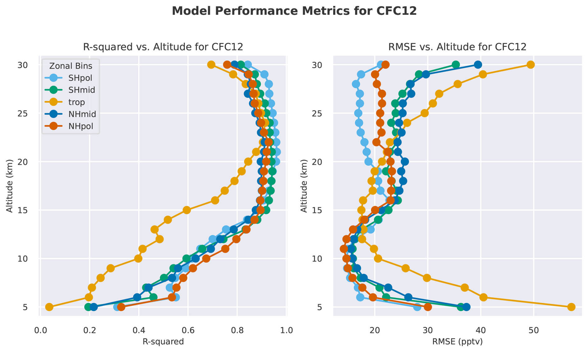
Figures 1 and 2 present the R² and RMSE values for all five latitude bands for CFC-11 and CFC-12, respectively, using the XGBoost regression model. For most latitude bands, the lowest possible altitude is about 5 km, and the top altitude ranges from 25 km (for CFC-11) to about 30 km (for CFC-12). Overall, the R² values are generally better for the polar and mid-latitude bins (SHpol, SHmid, NHmid, NHpol) compared to the tropical latitude bin (Trop). The Trop bin exhibits the lowest R² values, however, the tropical band also shows the smallest RMSE values for tropospheric levels (below 18 km). This seemingly contradictory result can be attributed to three main factors affecting the prediction model's performance in the tropics:

1. Limited data availability: The SCISAT-1 satellite, which carries the ACE-FTS instrument, is in a high-inclination (74°) orbit. This orbital path naturally concentrates measurements at high and middle latitudes. Consequently, the tropical stratosphere has significantly fewer measurements (∼ 21 000 measurements) compared to the polar/mid-latitude regions (∼ 45 000). For tropospheric levels, the number of valid measurements for the tropical bands is even lower (∼ 4000), most likely due to the presence of thin layers of cirrus clouds near the tropical upper troposphere – lower stratosphere (UTLS) region, which impacts data retrieval quality.

2. High dynamical variability: The large dynamical variability associated with the younger AoA in the tropical stratosphere increases prediction complexity. This challenge is particularly pronounced in the troposphere and, to some extent, in the lower and middle stratosphere, making the relationship between the input features and the target variable less predictable.

3. Influence of chemical loss: The mid-to-high latitude distributions are controlled by a strong seasonal cycle in both horizontal transport from the tropics to high latitudes (e.g. Holton et al., 1995; Butchart and Scaife, 2001) and the downward transport of air that is CFC-poor (i.e., air that has experienced significant photolysis exposure) to lower levels. This dominant, annual transport mechanism in the mid-to-high latitudes results in a more robust fit for the XGBoost model, leading to higher R² values compared to the more complex tropical region.

Overall, the small RMSE values demonstrate that the absolute prediction errors remain low because the fundamental dynamical processes driving CFC VMRs are reasonably well-represented in TOMCAT. Conversely, the lower R² values are a result of the high dynamical variability and limited data availability in the tropics. In particular, at lower altitudes (below 17 km) ACE measures upper tropospheric VMRs, which makes it statistically more difficult for the model to explain a high proportion of the observed variance even when the absolute predictions are accurate.

5.1.1 CFC-11 Performance

For CFC-11, the performance of XGBoost in SHpol shows R² values exceeding 0.8 from approximately 12 to 21 km, with the best performance observed near 17 km (Fig. 1). Above 21 km, R² values decrease rapidly. This is likely because CFC-11 VMRs are much smaller at these higher altitudes, leading to fewer observations and potentially larger retrieval errors. In the tropical latitude bin, the best performance (R²∼0.9) is observed near 22 km, and R² values remain greater than 0.7 for nearly all altitudes above 10 km. As mentioned in Sect. 5.1, despite the lower R² values in the tropics, the RMSE errors remain below 15 pptv, suggesting that for this latitude band, the dynamical processes driving CFC-11 VMRs are reasonably well-represented in the TOMCAT model, which provides key features to the regression. The lowest RMSE values for all five latitude bands are observed near the UTLS region, indicating the ability of XGBoost to partially constrain dynamical variability in this region with large spatial and temporal variability that is caused by numerous competing transport, chemical, and mixing processes around the tropopause (e.g. Millán et al., 2023).

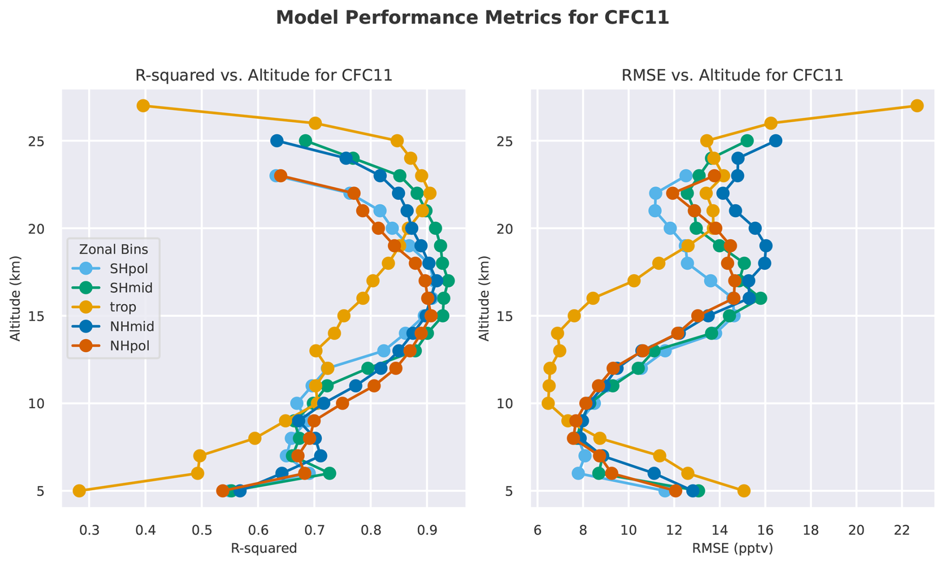
Figure 1 Coefficient of determination (R², left panel) and root mean squared error values (RMSE, right panel, in parts per trillion by volume (pptv)) for all 5-latitude bands from the XGBoost regression model.

5.1.2 CFC-12 Performance

The performance metrics for CFC-12 (Fig. 2) are generally better than those for CFC-11, with the tropical band being the exception. R² values for CFC-12 are close to 0.9 for altitudes ranging from 15 to 25 km and remain above 0.8 for most stratospheric levels. The differences in R² values between CFC-11 and CFC-12 (particularly in the tropical band) are noteworthy. Since both species have long atmospheric lifetimes (∼ 56 years for CFC-11 and ∼ 96 years for CFC-12, Chipperfield et al., 2014), they are co-emitted, and utilis e nearly identical feature matrices in XGBoost, so the discrepancies may be linked to differences in their loss processes. CFC-12 has a longer atmospheric lifetime and nearly double the concentration of CFC-11 (Hoffmann et al., 2014). Consequently, CFC-12 VMRs remain stable throughout most of the lower stratospheric levels. Furthermore, the CFC-12 model maintains high R² values over a more extended altitude range (up to 24 km) compared to CFC-11. This is most likely attributable to its photolytic loss occurring at higher altitudes, resulting in a more substantial and robust data set for training the regression model at mid-stratospheric levels (see Fig. 2).

Figure 2 Same as Fig. 1, but for CFC-12.

Additionally, vertical profiles of the retrieved CFC-11/CFC-12 mixing ratios (from ACE-FTS and the XGBoost model or TCOM) are compared with the original TOMCAT profiles in Supplement Figs. S3 and S4. The comparison, restricted to the 30 % test data points, clearly shows that the TCOM profiles show very good agreement with the ACE-FTS observations across all zonal latitude bins and valid vertical levels. However, at mid-stratospheric levels (the top levels where ACE-FTS retrieval of individual species is possible), the XGBoost-derived profiles appear to shift towards the original TOMCAT profiles. This behaviour suggests a limitation in the XGBoost model's predictive ability at these altitudes, which is likely driven by the rapid decrease in CFC VMRs. This decrease leads to very noisy CFC measurements (due to a poor signal-to-noise ratio in the satellite observations), resulting in a weakly trained and less constrained XGBoost model in the mid-stratosphere.

5.1.3 Feature Importance Across Altitudes

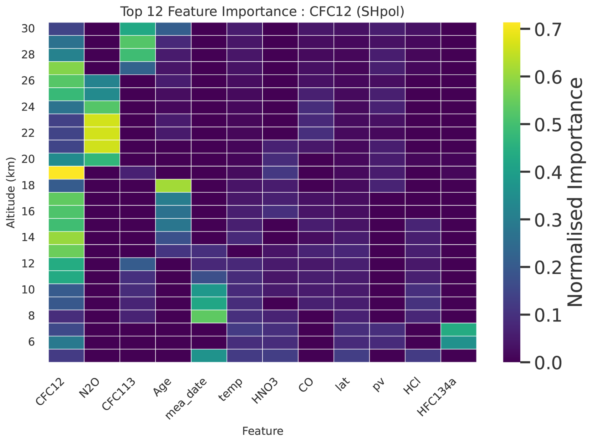
The feature importance analysis, shown as heatmaps for the SHpol band (Figs. 3 and 4), quantifies the overall influence of various variables or features on the XGBoost-predicted CFC-11 and CFC-12 VMRs. Feature importances for other latitude bands are shown in Supplement Figs. S5 to S12. Overall, for both CFC-11 and CFC-12 XGBoost selects nearly similar features for predicting the ACE-FTS measurements. The most important feature across all altitude and latitude bands is consistently the corresponding tracer from the TOMCAT CTM. This finding strongly suggests that the fundamental controlling processes for CFC VMRs, such as transport and chemical loss, are well-represented within the TOMCAT CTM. Beyond the primary TOMCAT tracer feature, the remaining features show subtle, altitude-dependent differences:

• For CFC-11, the second and third most important features are the AoA (a proxy for transport) in the 14–18 km range, and the measurement date in the 6–9 km range, which reflects both dynamical and chemical controls on tropospheric VMRs .

• For CFC-12, two transport tracers, N₂O and AoA, are selected within the 14–26 km altitude range, while the measurement date becomes more important below 10 km.

This general pattern remains consistent for low- to mid-latitude bands (e.g., SHmid, Trop, NHmid), where long-lived tracers (N₂O, CFC-113, HF, CFC-11, CFC-12) frequently appear as key secondary or tertiary features, particularly within the middle stratosphere. A notable exception is observed at higher latitudes (SHpol and NHpol), where the measurement date emerges as a somewhat important major feature, especially at lower (tropospheric) altitudes, compared to mid-low latitudes. The increased reliance on the measurement date at high latitudes suggests a deficiency in the TOMCAT simulation’s ability to fully capture variations driven by crucial dynamical processes, especially stratosphere-troposphere exchange (STE). At high latitudes, the primary transport process is the strong seasonal downward transport, resulting in the influx of CFC-poor air (due to stratospheric photolysis) from higher levels into the lower atmosphere, especially within the wintertime well-isolated polar vortex. This influx of older, CFC-depleted air likely requires the machine learning model to use the measurement date as an explicit correction term, indicating a need for TOMCAT to better resolve downward descent from high altitudes as well as horizontal mixing.

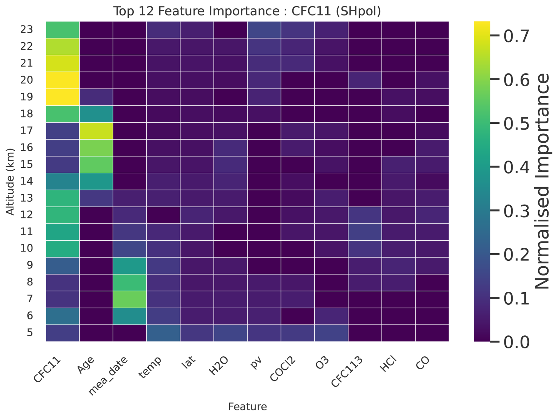
Figure 3 Normalised feature importance heatmap for CFC-11 in the Southern Hemisphere polar (SHpol) latitude bin, derived from the XGBoost regression model. The y-axis represents altitude (in km), and the x-axis lists the 12 most important input features. The colour intensity indicates the normalised relative importance of each feature at a specific altitude level for predicting the ACE-FTS CFC-11 VMR.

Figure 4 Same as Fig. 3 but for CFC-12 and different y-axis range, showing the altitude-dependent normalised relative importance of 12 most important features for the CFC-12 prediction.

5.2 Bias Correction Performance and SHAP Value Analysis

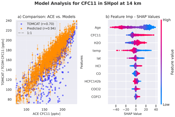
Scatterplots comparing the XGBoost-predicted (TCOM) and TOMCAT-simulated CFC-11 and CFC-12 performances with respect to ACE-FTS observations at 14 km for the SHpol latitude bin are shown in Figs. 5 and 6, respectively. Similar analyses for SHmid (16 km), Trop (18 km), NHmid (16 km), and NHpol (14 km) are shown in Supplement Figs. S13 to S20. These figures clearly demonstrate the effectiveness of the developed bias-correction methodology. The corrected TCOM data points (orange circles) are visibly clustered much closer to the 1:1 line compared to the TOMCAT data (blue circles), signifying a substantial reduction in systematic discrepancies. Pearson correlation coefficients, shown in the legend, also exhibit significant improvements. For example, in Fig. 5 r increases from 0.70 for TOMCAT to r=0.94 for TCOM, whereas in Fig. 6 it improves from r=0.61 to r=0.92. The TCOM data points also include estimated uncertainties derived using quantile regression (the 25th and 75th percentiles).

Figures 5 and 6 also show the SHAP (SHapley Additive exPlanations) values for the XGBoost model at 14 km. SHAP analysis is a crucial component of interpretable machine learning, providing a local, additive explanation for each prediction. Unlike the overall feature importance metric, SHAP values quantify the contribution of each input feature to a single, specific prediction, including the direction (positive or negative) of the influence.

The analysis of the SHAP values in Fig. 5b for CFC-11 at 14 km in the SHpol region provides a detailed look at how XGBoost functions as a transport corrector by applying specific adjustments based on the chemical and dynamical characteristics of different air masses. The results indicate that XGBoost is able to identify distinct regimes to rectify biases in the underlying TOMCAT fields. Age-of-Air is identified as the most influential dynamical feature, where high values representing photochemically aged air that has descended from the mid-to-upper stratosphere are associated with negative SHAP values reaching −50 pptv. Conversely, younger air masses receive positive adjustments of up to +40 pptv. The simulated TOMCAT CFC-11 tracer concentration itself also plays a major role; air masses where TOMCAT-simulated VMRs are relatively high, typically representing air transported from lower latitudes, receive positive corrections of approximately +40 pptv, while very little adjustment occurs at lower concentration levels. Other features also help to characterise these regimes. For example, air masses with high water vapour and warmer temperatures receive negative adjustments, whereas corresponding air with low water vapour (a sign of dehydrated vortex air), and colder conditions receive positive adjustments. These patterns suggest that the largest downward adjustments occur when the air is older and drier, indicating that TOMCAT tends to overestimate residual small CFC VMRs in heavily photochemically aged air descended during winter. This typically occurs near the polar vortex edge or after breakup where simulated vertical descent and horizontal mixing are not fully captured in the raw TOMCAT fields.

Similar distinct adjustment patterns are observed for CFC-12 as shown in Fig. 6b, where the tracer concentration, Age-of-Air, and temperature are the most influential features. Air masses with a high Age-of-Air and low simulated TOMCAT VMRs are strongly associated with negative SHAP values, reaching approximately −50 and −40 pptv, respectively. This confirms a downward adjustment to the XGBoost predicted mixing ratios, suggesting that TOMCAT also tends to overestimate residual CFC-12 in aged air that has descended within the polar vortex. In contrast, low temperatures, which are a defining characteristic of the cold polar stratosphere, drive large positive corrections of up to +60 pptv. This highlights how the model utilises thermodynamic signatures to rectify deficiencies in the simulated stratospheric circulation and its representation in meteorological reanalyses.

The scatterplots and SHAP analyses for the remaining latitude bands, provided in Supplement Figs. S13 to S20, confirm the global robustness and consistency of the TCOM framework. Across all latitude bins – SHmid (16 km), Trop (18 km), NHmid (16 km), and NHpol (14 km) – the corrected TCOM data points consistently exhibit a tighter clustering around the 1:1 line, with significant improvements in Pearson correlation coefficients relative to the baseline TOMCAT simulations. Consistent with the SHpol analysis, the SHAP results for these regions identify the corresponding TOMCAT tracer as a major predictor, though in the tropical upper troposphere (Fig. S15), other features such as CFC-113 and temperature exhibit higher relative importance. Additionally, the high relative influence of dynamical features such as Age-of-Air, temperature, and potential vorticity across all latitude bins underscores the model's role in rectifying circulation-driven biases. In the Trop region (Figs. S15 and S16), where dynamical variability is large and observational constraints are relatively sparse, TCOM effectively resolves notable TOMCAT offsets, with correlation coefficients improving from 0.82 to 0.93 for CFC-11 and 0.76 to 0.89 for CFC-12. In the NHmid and NHpol regions (Figs. S17 to S20), the bias-correction patterns mirror those observed in the SH, reinforcing the conclusion that the TCOM methodology successfully harmonises sparse satellite observations with continuous model background fields across range of atmospheric regimes.

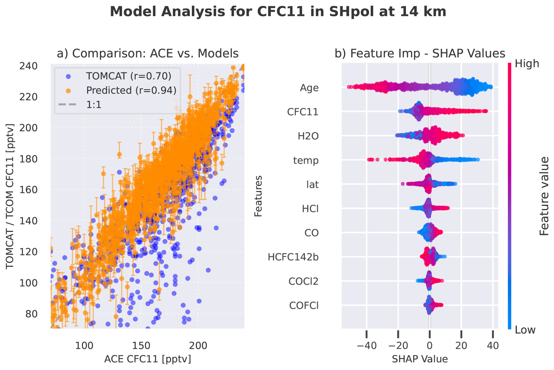
Figure 5 (a) Comparison of CFC-11 VMRs (in parts per trillion by volume or pptv) at 14 km altitude in the Southern Hemisphere polar (SHpol) latitude band. The scatter plot compares ACE-FTS observations (horizontal axis) against the model output: TOMCAT CTM (blue circles) and XGBoost regression model estimated VMRs (TCOM, orange circles). The vertical lines on the TCOM data represent the estimated uncertainties derived using quantile regression (25th and 75th percentiles). The dashed grey line indicates the 1:1 line to illustrate deviations with respect to ACE-FTS data. The legend also includes the Pearson correlation between ACE-FTS and the TOMCAT or TCOM data. (b) SHAP (SHapley Additive exPlanations) values for the XGBoost model at the same level (14 km). The SHAP values indicate the relative importance of each input feature and the direction (positive or negative) of their influence on the XGBoost model's prediction (corrected as TCOM).

Figure 6 Same as Fig. 5, but for CFC-12.

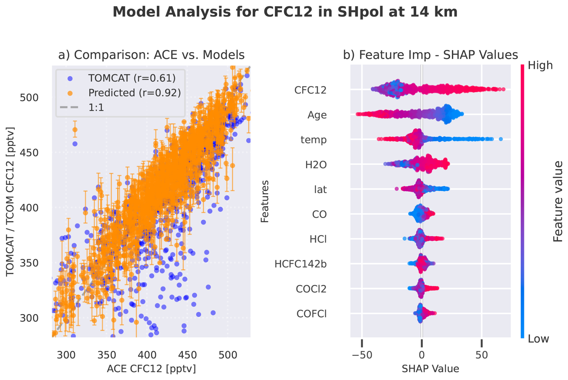
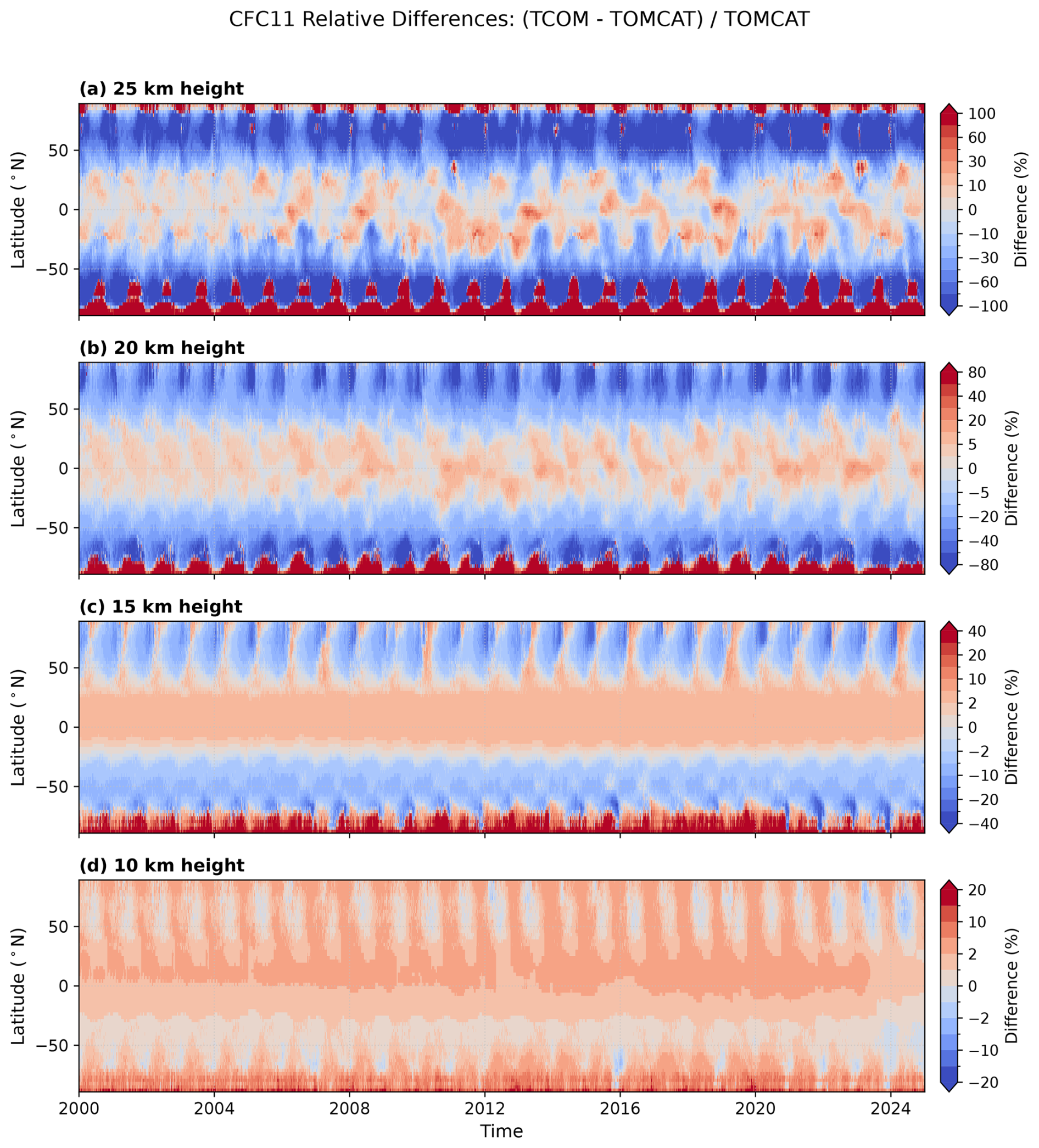
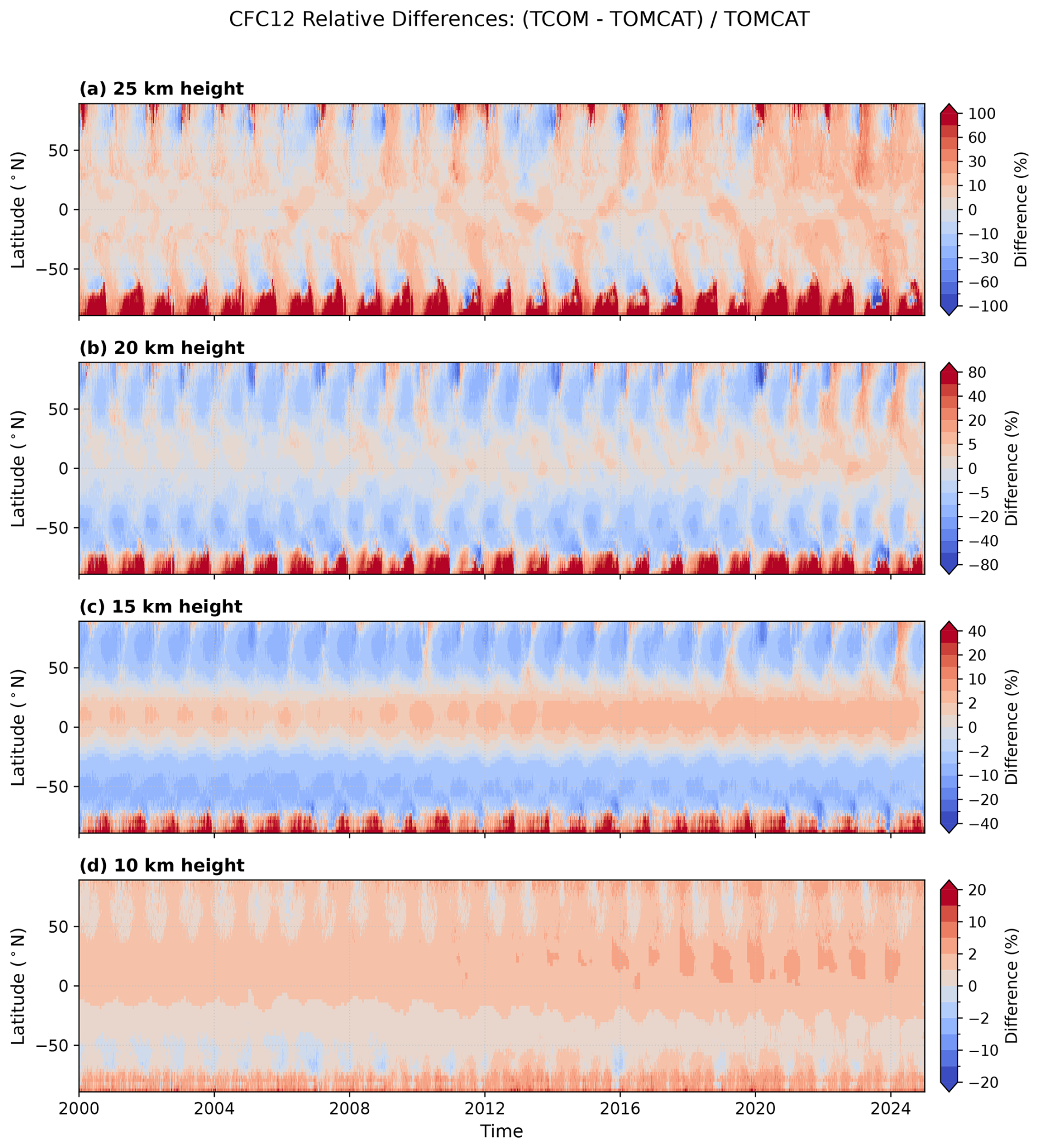
Figure 7 Percentage differences between the TCOM and TOMCAT VMRs of CFC-11 as a function of time (2000–2024) and latitude (85° S to 85° N). Differences are presented for four altitude levels: 25 km (top panel), 20, 15, and 10 km (bottom panel). The differences are calculated as $\mathrm{100}\times (\mathrm{TCOM}-\mathrm{TOMCAT})/\mathrm{TOMCAT}$. The colour-bar scales for the percentage difference are irregular and optimised for each individual altitude panel.

Figure 8 Same as Fig. 7, but for CFC-12, comparing TOMCAT and TCOM data.

5.3 Analysis of TCOM vs TOMCAT Differences

We now analyse percentage differences between TCOM and TOMCAT VMRs for CFC-11 and CFC-12. Figures 7 and 8 reveal distinct patterns in the corrections estimated by the XGBoost model across different altitudes, latitudes, and time. A common feature for both CFC-11 and CFC-12 is the presence of large positive and negative percentage differences at different levels, particularly in the high-latitude regions (south of 60° S and north of 60° N); where XGBoost seems to adjust TCOM profiles upwards at upper levels (above 10–15 km). Also, at mid-high latitudes (≥  40°), XGBoost seems to remove positive biases in TOMCAT at lower levels. Overall, largest corrections are applied at higher altitudes (25 and 20 km) in the tropics and for all levels at extreme high latitudes (≥ 70°). This indicates that the XGBoost correction, as captured in the TCOM dataset, introduces relatively large adjustments compared to the TOMCAT baseline, especially in areas characterised by polar vortex dynamics and seasonal transport coinciding with extreme polar events, such as the anomalous Antarctic winter of 2002 (e.g. Weber et al., 2003) or the severe Arctic winters in 2020 (e.g. Feng et al., 2021) and 2024 (e.g. Newman et al., 2024). The extreme correction, sometimes exceeding ±80 % or even ±100 % in the 25 km panel for CFC-12, underscores the magnitude of the correction needed in these chemically and dynamically active lower-middle stratospheric levels.

At lower altitudes, specifically 15 and 10 km, the scale of the percentage differences for both CFC-11 and CFC-12 decreases substantially at low-mid latitudes as CFCs are more abundant in this region. For these latitudes (≤ 60°) maximum differences are generally constrained to ±40 % and ±20 % at 15 and 10 km, respectively. This suggests that TOMCAT's performance, when compared to the TCOM product, is more consistent in the lower stratosphere, implying that the fundamental chemical and transport processes for these CFCs are reasonably well simulated by the CTM in this region. However, distinct geographical and temporal patterns persist. At 10 km, a band of sustained positive difference is visible across the tropical and mid-latitude regions (50° S to 50° N) throughout the entire 2000–2024 period for both CFCs. This implies a consistent, relatively small but persistent underestimation of CFC VMRs by TOMCAT in the tropical lower stratosphere, which XGBoost effectively rectifies. This persistent difference may stem from TOMCAT’s photolysis loss occurring mainly at tropical middle -lower stratosphere, whereas observations suggest that similar losses should occur at higher altitudes as well. Also, an interesting feature at lower altitudes is the inter-hemispheric asymmetry at low-mid latitudes. Persistent positive bands of difference are observed from the tropics to the NH mid-latitudes, particularly between 10 and 15 km (see Figs. 7 and 8). This appears to be consistent with the results of Schmidt et al. (2024), who analysed ACE-FTS data sets for various long-lived species and identified a distinct hemispheric asymmetry. They found that SH VMRs in the lower stratosphere exhibit a 2.25-year lag compared to those in the NH. They noted similar lags in NOAA surface observations and suggested that these differences may be linked to the concentration of industrial emissions in the NH, the time required for these changes to mix thoroughly into the measured atmospheric regions, or a combination of complex vertical and horizontal transport pathways. Furthermore, the strong gradient in differences near the edge of the polar vortex (especially in the SHpol region) indicates that horizontal transport is likely too constrained in the TOMCAT simulation across almost all levels.

Additionally, there are noticeable differences in the correction pattern between the two compounds. For CFC-12, the regions of very large percentage differences at 25 km appear more concentrated and tightly coupled with the seasonal cycle in the polar regions, suggesting a stronger influence of the polar vortex and associated transport processes. In contrast, the CFC-11 plots show a broader, albeit still high-magnitude, correction pattern at 25 km, with notable positive differences extending into the mid-latitudes across the entire time series. This may reflect differences in the photochemical lifetimes (e.g. Chipperfield et al., 2014; Hoffmann et al., 2014) and vertical distribution of the two CFCs, leading to distinct sensitivities in the XGBoost corrections.

On a long-term basis (2000 to 2024), there is minor but systematic divergence in the correction patterns for both species. For the top three levels, differences seem to grow larger with time, with the largest corrections estimated for recent years, which coincide with record minimum or maximum springtime ozone observations. The exact causes of these diverging patterns are not fully understood. However, unusual changes in stratospheric composition (e.g., the Australian New Year (ANY) fires in 2020 or the Hunga eruption in 2022) might have caused changes in stratospheric circulation that were not accurately captured by the ERA5 reanalysis data used to drive TOMCAT. We aim to analyse these patterns in future studies.

5.4 Comparison with SPARC Data

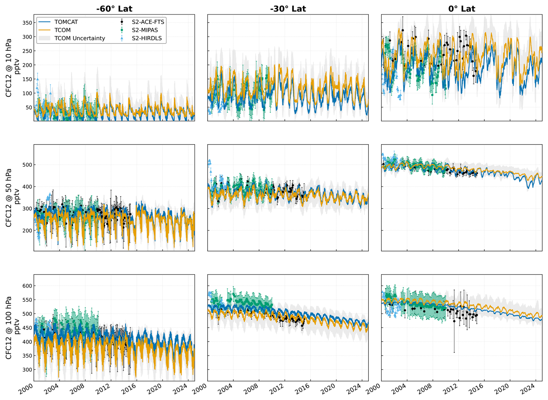
A critical evaluation of the TCOM dataset is provided through comparisons with independent observation-based products from the SPARC v2 compilation (Hegglin et al., 2021), and is presented in Fig. 9 for CFC-11 and Fig. 10 for CFC-12. To ensure clarity in the figures and to analyse different dynamical regimes in detail, we focus on the three representative latitude bins: high-latitude (SHpol, 60° S), subtropical (30° S), and tropical (0°), across three stratospheric pressure levels (100, 50, and 10 hPa).

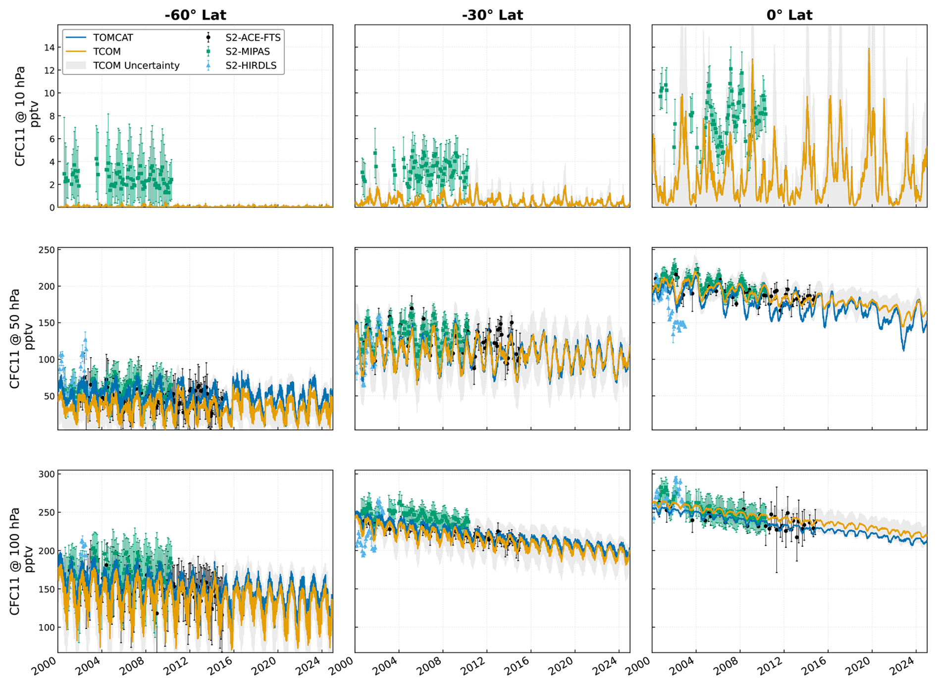
Figure 9 Temporal comparison of daily-mean CFC-11 VMRs (in pptv) from 2000 to 2024 across three distinct latitudes (60° S, 30° S and 0°) at three stratospheric pressure levels: 10 hPa (≈ 30 km), 50 hPa (≈ 20 km), and 100 hPa (≈ 16 km). Data sources shown include: the TOMCAT CTM output (solid blue lines), the XGBoost-predicted TCOM dataset (solid orange lines), and TCOM uncertainty (±1σ derived from quantile regression, light orange shading). Monthly mean data points from observation-based data from the SPARC v2 (Hegglin et al., 2021) are also shown. Data points and related standard deviations from ACE-FTS, MIPAS and HIRDLS are shown with black, green and aqua coloured dots, respectively.

Figure 10 Same as Fig. 9, but for CFC-12.

In the middle stratosphere at 50 hPa, a systematic low bias in raw TOMCAT output is most evident, particularly in the tropical and subtropical panels. This consistent offset suggests that while TOMCAT accurately represents the large-scale declining trend, it does not fully capture the vertical gradient of these long-lived species, possibly due to weaker photolysis in the tropics and model deficiencies in representing the horizontal mixing of CFC-rich air from the tropical pipe into mid-latitudes. The TCOM correction successfully resolves this bias, aligning the mixing ratios with the satellite-observations-based SPARC v2 monthly mean data points.

5.4.1 CFC-11 Comparison Analysis

The CFC-11 comparison in Fig. 9 highlights the efficacy of the machine learning approach across varying dynamical regimes:

• Tropics (0°): At 100 and 50 hPa, TOMCAT exhibits a significant negative bias relative to the high-density cluster of ACE-FTS, MIPAS, and HIRDLS measurements. TCOM effectively bridges this gap, while at the highly variable 10 hPa level, it tracks the sparse satellite scatter and captures the long-term decline indicated by MIPAS.

• Subtropics (30° S): The 100 hPa panel shows very good agreement across all datasets, confirming that model-simulated stratosphere-troposphere exchange (STE) is broadly correct in this region. At 100 and 50 hPa, TCOM applies minor downward and upward adjustments, respectively, and it matches the key features in SPARC ACE-FTS data points, and also identifies a persistent high bias in the MIPAS data points relative to the ACE-FTS.

• Mid-high latitudes (60° S): Strong seasonal oscillations are visible at 100 hPa, where TCOM adjusts downwards to match observational constraints. At the 50 hPa level, the XGBoost correction is vital for rectifying the overestimation of TOMCAT values during winter correcting either weaker polar descent or horizontal mixing near the edge of the vortex, ensuring the final product accurately reflects the chemically processed air within the high-latitude vortex.

5.4.2 CFC-12 Comparison Analysis

Similar robust improvements are observed for CFC-12 in Fig. 10, which benefits from better retrievals at higher altitudes:

• Tropics (0°): The 100 hPa tropical panel shows the most prominent deficiencies in TOMCAT data, which is systematically removed in TCOM to match the SPARC data points. At 50 hPa, the adjustment is minor. At 10 hPa, where natural variability is highest, TCOM introduces daily fluctuations that successfully mirrors the dynamic cycle captured by MIPAS and ACE-FTS.

• Subtropics (30° S): At 100 hPa all the data sets confirm declining trends and TCOM shows downward adjustment to match SPARC data points. The 50 hPa level reveals that TCOM remains centred within the ACE-FTS scatter (black dots), consistently staying within uncertainty estimates while TOMCAT data suggests very little adjustment is needed.

• Mid-high latitudes (60° S): The polar panels also show that TCOM data points remain close to the SPARC ACE-FTS data points. At 100 and 50 hPa, the downward correction accounts for the TOMCAT's inability to fully simulate the descent of older air (or horizontal mixing), bringing TCOM into better alignment with both MIPAS and ACE-FTS monthly means. On the other hand, at 10 hPa upward adjustment is needed to match SPARC data points.

Overall, this intercomparison confirms that while different satellite measurements are generally consistent in the lower stratosphere, the TCOM dataset provides unique added value by statistically harmonising continuous model output with these rigorous observational constraints, resulting in a consistent and high-fidelity global record

6 Data availability

The TCOM version 2.0 datasets are publicly available on Zenodo. While the initial methodology for version 1.0 was detailed in Dhomse and Chipperfield (2023) focusing on CH₄ and N₂O, the current v2.0 products described in this study have been expanded to include a range of stratospheric species. Specifically, the datasets for CFC-11 and CFC-12 can be accessed at https://doi.org/10.5281/zenodo.18145730 (Dhomse, 2026a) and https://doi.org/10.5281/zenodo.18147392 (Dhomse, 2026b), respectively. Using the same methodology, v2.0 profile datasets are also publicly available for O₃ (https://doi.org/10.5281/zenodo.18199586, Dhomse, 2026c), H₂O (https://doi.org/10.5281/zenodo.18199962, Dhomse, 2026d), CH₄ (https://doi.org/10.5281/zenodo.18197333, Dhomse, 2026e), N₂O (https://doi.org/10.5281/zenodo.18197444, Dhomse, 2026f), HF (https://doi.org/10.5281/zenodo.18184779, Dhomse, 2026g), HCl (https://doi.org/10.5281/zenodo.18184430, Dhomse, 2026h), HNO₃ (https://doi.org/10.5281/zenodo.18199002, Dhomse, 2026i), and COF₂ (https://doi.org/10.5281/zenodo.18201786, Dhomse, 2026j). These links are all listed and maintained on the overview TCOM page (https://tomcat.leeds.ac.uk/tomcat/tcom, last access: July 2026).

The ACE-FTS v5.3 data utilised for these TCOM constraints are available at the official archive: https://databace.scisat.ca (last access: 14 March 2025). Additional daily 3D profile fields, for both TOMCAT and TCOM are available from the corresponding author upon request.

7 Summary and Conclusions

We present the TCOM-CFC11 and TCOM-CFC12 (v2.0) datasets, which provide continuous, gap-free, global daily vertical profiles of CFC VMRs from 2000 to 2024. This was achieved using an innovative methodology that employs XGBoost regression to constrain the continuous output of the TOMCAT CTM against high-quality ACE-FTS satellite observations, thereby addressing the limitations of sparse satellite coverage. The comparative analysis demonstrated the method's effectiveness, as the corrected TCOM data clustered significantly closer to the observations, effectively removing the systematic low bias present in TOMCAT in the middle stratosphere (e.g., at 50 hPa) when validated against independent observation-based products such as the SPARC v2 data set.

The analysis of model diagnostics, particularly the SHAP values, provided crucial insight into the physical origin of the deficiencies of the TOMCAT simulation. The feature importance investigation strongly suggests that the XGBoost regression model functions primarily as a “transport corrector”. This is evidenced by the high influence of dynamical features, such as age-of-air (AoA) and potential vorticity (PV), indicating that the main source of model bias relates to how TOMCAT simulates stratospheric circulation, rather than its chemical schemes. This transport correction is most notable in the polar regions, where TCOM rectifies a systematic underestimation in TOMCAT. The most probable reason is likely to be errors in transport-related parameters in TOMCAT or biases in the representation of the stratospheric circulation in the ERA5 reanalysis fields that are used to drive the model.

In conclusion, the TCOM datasets successfully harmonise the TOMCAT CTM output with rigorous observational constraints, yielding a consistent, high-fidelity resource for the stratospheric research community. Version 2.0 incorporates the latest ACE-FTS v5.3 data and provides robust uncertainty estimates derived from ensemble retraining using the 25th and 75th percentiles of observations. The final TCOM-CFC11 and TCOM-CFC12 datasets are (since January 2026) publicly released and will serve as a valuable, observationally-constrained benchmark for evaluating and refining CTMs and CCMs, helping to reduce uncertainties in long-term trend analyses of ozone-depleting substances, and aiding in the assessment of the Montreal Protocol's effectiveness.

Finally, while the current version of the TCOM dataset relies on the high-quality constraints provided by ACE-FTS, the methodology is designed to be adaptable to future observational streams. The upcoming ALICE instrument on NASA STRIVE mission (to be launched in early 2030s), with its ability to measure vertical profiles for a wide range of trace gases, including both CFCs and other species currently included in the TCOM datasets (e.g. O₃, CH₄, N₂O, HNO₃, H₂O), will offer a critical opportunity to maintain and extend these gap-free data records well into the next decade. Within the current framework, we have shown that even with a data gap (e.g. 2000 to 2003 in this study) profile data sets can be constructed for most of the long-lived species based on the chemical-dynamical information derived during the observed period. Extrapolations based on gradually varying source gas loadings, e.g. obtainable from ground-based observations, can be accommodated. The most problematic issue would be sudden atmospheric perturbations such as the changes in the stratospheric aerosol properties due to volcanic eruptions or wildfires for which direct aerosol observations are needed. Nonetheless, future trace observations from missions such as STRIVE are essential to provide reference anchor points for the end of a gap-filled period.