Global Carbon Budget 2024

Accurate assessment of anthropogenic carbon dioxide (CO₂) emissions and their redistribution among the atmosphere, ocean, and terrestrial biosphere in a changing climate is critical to better understand the global carbon cycle, support the development of climate policies, and project future climate change. Here we describe and synthesize datasets and methodologies to quantify the five major components of the global carbon budget and their uncertainties. Fossil CO₂ emissions (E_FOS) are based on energy statistics and cement production data, while emissions from land-use change (E_LUC) are based on land-use and land-use change data and bookkeeping models. Atmospheric CO₂ concentration is measured directly, and its growth rate (G_ATM) is computed from the annual changes in concentration. The global net uptake of CO₂ by the ocean (S_OCEAN, called the ocean sink) is estimated with global ocean biogeochemistry models and observation-based fCO₂ products (fCO₂ is the fugacity of CO₂). The global net uptake of CO₂ by the land (S_LAND, called the land sink) is estimated with dynamic global vegetation models. Additional lines of evidence on land and ocean sinks are provided by atmospheric inversions, atmospheric oxygen measurements, and Earth system models. The sum of all sources and sinks results in the carbon budget imbalance (B_IM), a measure of imperfect data and incomplete understanding of the contemporary carbon cycle. All uncertainties are reported as ±1σ.

For the year 2023, E_FOS increased by 1.3 % relative to 2022, with fossil emissions at 10.1 ± 0.5 GtC yr⁻¹ (10.3 ± 0.5 GtC yr⁻¹ when the cement carbonation sink is not included), and E_LUC was 1.0 ± 0.7 GtC yr⁻¹, for a total anthropogenic CO₂ emission (including the cement carbonation sink) of 11.1 ± 0.9 GtC yr⁻¹ (40.6 ± 3.2 GtCO₂ yr⁻¹). Also, for 2023, G_ATM was 5.9 ± 0.2 GtC yr⁻¹ (2.79 ± 0.1 ppm yr⁻¹; ppm denotes parts per million), S_OCEAN was 2.9 ± 0.4 GtC yr⁻¹, and S_LAND was 2.3 ± 1.0 GtC yr⁻¹, with a near-zero B_IM (−0.02 GtC yr⁻¹). The global atmospheric CO₂ concentration averaged over 2023 reached 419.31 ± 0.1 ppm. Preliminary data for 2024 suggest an increase in E_FOS relative to 2023 of +0.8 % (−0.2 % to 1.7 %) globally and an atmospheric CO₂ concentration increase by 2.87 ppm, reaching 422.45 ppm, 52 % above the pre-industrial level (around 278 ppm in 1750). Overall, the mean of and trend in the components of the global carbon budget are consistently estimated over the period 1959–2023, with a near-zero overall budget imbalance, although discrepancies of up to around 1 GtC yr⁻¹ persist for the representation of annual to semi-decadal variability in CO₂ fluxes. Comparison of estimates from multiple approaches and observations shows the following: (1) a persistent large uncertainty in the estimate of land-use change emissions, (2) low agreement between the different methods on the magnitude of the land CO₂ flux in the northern extra-tropics, and (3) a discrepancy between the different methods on the mean ocean sink.

This living-data update documents changes in methods and datasets applied to this most recent global carbon budget as well as evolving community understanding of the global carbon cycle. The data presented in this work are available at https://doi.org/10.18160/GCP-2024 (Friedlingstein et al., 2024).

1 Introduction

The concentration of carbon dioxide (CO₂) in the atmosphere has increased from approximately 278 parts per million (ppm) in 1750 (Gulev et al., 2021), the beginning of the industrial era, to 419.3 ± 0.1 ppm in 2023 (Lan et al., 2024; Fig. 1). The atmospheric CO₂ increase above pre-industrial levels was, initially, primarily caused by the release of carbon to the atmosphere from deforestation and other land-use change activities (Canadell et al., 2021). While emissions from fossil fuels started before the industrial era, they became the dominant source of anthropogenic emissions to the atmosphere from around 1950, and their relative share has continued to increase until the present. Anthropogenic emissions occur on top of an active natural carbon cycle that circulates carbon between the reservoirs of the atmosphere, ocean, and terrestrial biosphere on timescales from sub-daily to millennial, while exchanges with geologic reservoirs occur on longer timescales (Archer et al., 2009).

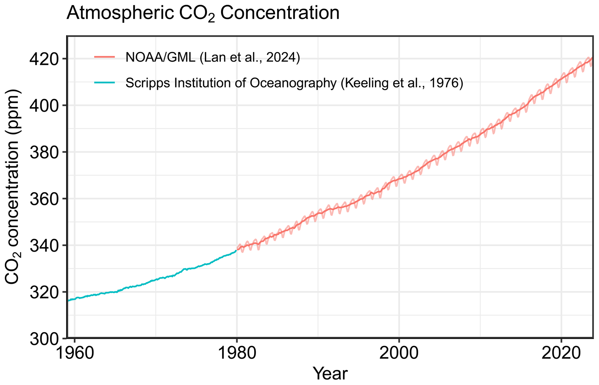
Figure 1 Surface average atmospheric CO₂ concentration (ppm). From 1980, monthly data are from NOAA/GML (Lan et al., 2024) and are based on an average of direct atmospheric CO₂ measurements from multiple stations in the marine boundary layer (Masarie and Tans, 1995). The 1958–1979 monthly data are from Scripps Institution of Oceanography, based on an average of direct atmospheric CO₂ measurements from the Mauna Loa and South Pole stations (Keeling et al., 1976). To account for the difference in mean CO₂ and seasonality between the NOAA/GML and the Scripps station networks used here, the Scripps surface average (from two stations) was de-seasonalized and adjusted to match the NOAA/GML surface average (from multiple stations) by adding the mean difference of 0.667 ppm, calculated here from overlapping data during 1980–2012.

The global carbon budget (GCB) presented here refers to the mean of, variations in, and trends in the perturbation of CO₂ in the environment, referenced to the beginning of the industrial era (defined here as 1750). This paper describes the components of the global carbon cycle over the historical period, with a stronger focus on the recent period (since 1958, onset of robust atmospheric CO₂ measurements), the last decade (2014–2023), the last year (2023), and the current year (2024) at the time of writing. Finally, it provides cumulative emissions from fossil fuels and land-use change since the year 1750 and since the year 1850 (the reference year for historical simulations in the Intergovernmental Panel on Climate Change Sixth Assessment Report, IPCC AR6) (Eyring et al., 2016).

We quantify the input of CO₂ to the atmosphere by emissions from human activities; the growth rate of atmospheric CO₂ concentration; and the resulting changes in the storage of carbon in the land and ocean reservoirs in response to increasing atmospheric CO₂ levels, climate change, and variability and other anthropogenic and natural changes (Fig. 2). An understanding of this perturbation budget over time and the underlying variability in and trends of the natural carbon cycle is necessary to understand the response of natural sinks to changes in climate, CO₂, and land-use change drivers and to quantify emissions compatible with a given climate stabilization target.

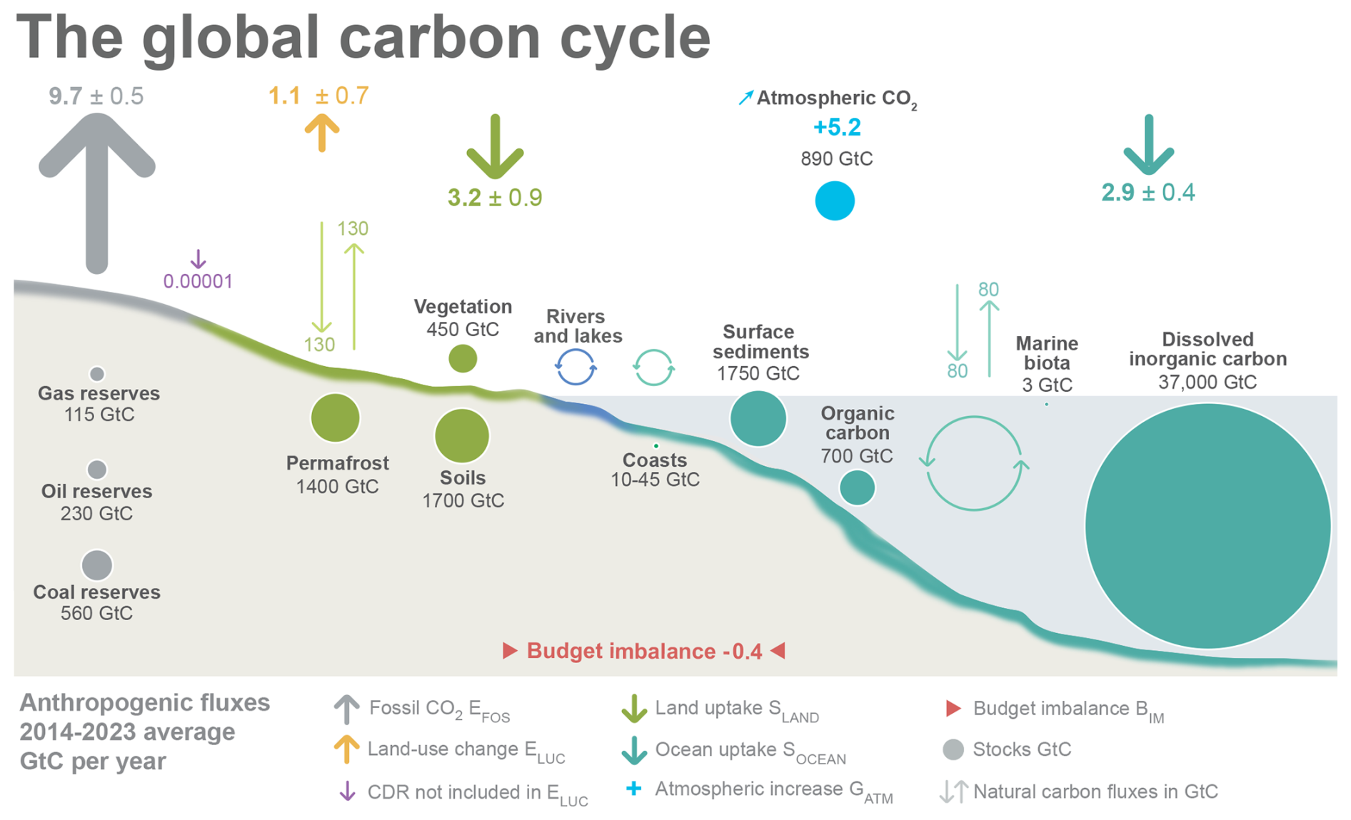
Figure 2 Schematic representation of the overall perturbation of the global carbon cycle caused by anthropogenic activities, averaged globally for the decade 2014–2023. See legend for the corresponding arrows. Flux estimates and their 1 standard deviation uncertainty are as reported in Table 7. The CDR estimate is for the year 2023 only. The uncertainty in the atmospheric CO₂ growth rate is very small (±0.02 GtC yr⁻¹) and is neglected for the figure. The anthropogenic perturbation occurs on top of an active carbon cycle, with fluxes and stocks represented in the background and taken from Canadell et al. (2021) for all numbers, except for the carbon stocks in coasts, which is from a literature review of coastal marine sediments (Price and Warren, 2016). Fluxes are in gigatonnes of carbon per year (GtC yr⁻¹) and reservoirs in gigatonnes of carbon (GtC). This figure was produced by Nigel Hawtin.

The components of the CO₂ budget that are reported annually in this paper include separate and independent estimates for the CO₂ emissions from (1) fossil fuel combustion and oxidation from all energy and industrial processes, also including cement production and carbonation (E_FOS; GtC yr⁻¹), and (2) deliberate human activities on land, including those leading to land-use change (E_LUC; GtC yr⁻¹), and their partitioning among (3) the growth rate of atmospheric CO₂ concentration (G_ATM; GtC yr⁻¹) and the uptake of CO₂ (the “CO₂ sinks”) in (4) the ocean (S_OCEAN; GtC yr⁻¹) and (5) on land (S_LAND; GtC yr⁻¹). The CO₂ sinks as defined here conceptually include the response of the land (including inland waters and estuaries) and ocean (including coastal and marginal seas) to elevated CO₂ and changes in climate and other environmental conditions, although in practice not all processes are fully accounted for (see Sect. 2.10). Note that the term sink means that the net transfer of carbon is from the atmosphere to land or the ocean, but it does not imply any permanence of that sink in the future. Global emissions and their partitioning among the atmosphere, ocean, and land are in balance in the real world. Due to the combination of imperfect spatial and/or temporal data coverage, errors in each estimate, and smaller terms not included in our budget estimate (discussed in Sect. 2.10), the independent estimates (1) to (5) above do not necessarily add up to zero. We hence estimate a budget imbalance (B_IM), which is a measure of the mismatch between the estimated emissions and the estimated changes in the atmosphere, land, and ocean, as follows:

$$\begin{array}{}\text{(1)}& B_{\mathrm{IM}}=E_{\mathrm{FOS}}+E_{\mathrm{LUC}}-(G_{\mathrm{ATM}}+S_{\mathrm{OCEAN}}+S_{\mathrm{LAND}}).\end{array}$$

G_ATM is usually reported in ppm yr⁻¹, which we convert to units of carbon mass per year, GtC yr⁻¹, using 1 ppm = 2.124 GtC (Ballantyne et al., 2012; Table 1). Units of gigatonnes of CO₂ (or billion tonnes of CO₂) used in policy are equal to 3.664 multiplied by the value in units of gigatonnes of carbon (GtC).

Table 1 Factors used to convert carbon in various units (by convention, unit 1 = unit 2 × conversion).

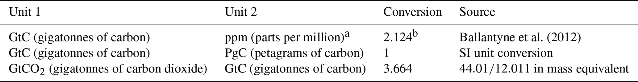
^a Measurements of atmospheric CO₂ concentration have units of dry-air mole fraction; “ppm” is an abbreviation for micromoles per mole, dry air. ^b The use of a factor of 2.124 assumes that all the atmosphere is well mixed within 1 year. In reality, only the troposphere is well mixed and the growth rate of CO₂ concentration in the less well mixed stratosphere is not measured by sites from the NOAA network. Using a factor of 2.124 gives an approximation that the growth rate of CO₂ concentration in the stratosphere equals that of the troposphere on a yearly basis.

We also assess a set of additional lines of evidence derived from global atmospheric inversion system results (Sect. 2.7), observed changes in oxygen concentration (Sect. 2.8), and Earth system model (ESM) simulations (Sect. 2.9), with all of these methods closing the global carbon balance (zero B_IM).

We further quantify E_FOS and E_LUC by country, including both territorial and consumption-based accounting for E_FOS (see Sect. 2), and discuss missing terms from sources other than the combustion of fossil fuels (see Sects. 2.10 and S1 and S2 in the Supplement). We also assess carbon dioxide removal (CDR) (see Sect. 2.2 and 2.3). Land-based CDR is significant but already accounted for in E_LUC in Eq. (1) (Sect. 3.2.2). Other CDR methods, not based on vegetation, are currently several orders of magnitude smaller than the other components of the budget (Sect. 3.3); hence these are not included in Eq. (1) or in the global carbon budget tables or figures (with the exception of Fig. 2, where CDR is shown primarily for illustrative purposes).

The global CO₂ budget has been assessed by the Intergovernmental Panel on Climate Change (IPCC) in all assessment reports (Prentice et al., 2001; Schimel et al., 1995; Watson et al., 1990; Denman et al., 2007; Ciais et al., 2013; Canadell et al., 2021) and by others (e.g. Ballantyne et al., 2012). The Global Carbon Project (GCP; https://www.globalcarbonproject.org/, last access: 21 January 2025) has coordinated this cooperative community effort for the annual publication of global carbon budgets for the year 2005 (Raupach et al., 2007; including fossil emissions only), year 2006 (Canadell et al., 2007), year 2007 (GCP, 2007), year 2008 (Le Quéré et al., 2009), year 2009 (Friedlingstein et al., 2010), year 2010 (Peters et al., 2012), year 2012 (Le Quéré et al., 2013; Peters et al., 2013), year 2013 (Le Quéré et al., 2014), year 2014 (Le Quéré et al., 2015a; Friedlingstein et al., 2014), year 2015 (Jackson et al., 2016; Le Quéré et al., 2015b), year 2016 (Le Quéré et al., 2016), year 2017 (Le Quéré et al., 2018a; Peters et al., 2017a), year 2018 (Le Quéré et al., 2018b; Jackson et al., 2018), year 2019 (Friedlingstein et al., 2019; Jackson et al., 2019; Peters et al., 2020), year 2020 (Friedlingstein et al., 2020; Le Quéré et al., 2021), year 2021 (Friedlingstein et al., 2022a; Jackson et al., 2022), year 2022 (Friedlingstein et al., 2022b), and most recently year 2023 (Friedlingstein et al., 2023). Each of these papers updated previous estimates with the latest available information for the entire time series.

We adopt a range of ±1 standard deviation (σ) to report the uncertainties in our global estimates, representing a likelihood of 68 % that the true value will be within the provided range if the errors have a Gaussian distribution, and no bias is assumed. This choice reflects the difficulty of characterizing the uncertainty in the CO₂ fluxes between the atmosphere and the ocean and land reservoirs individually, particularly on an annual basis, as well as the difficulty of updating the CO₂ emissions from land-use change. A likelihood of 68 % provides an indication of our current capability to quantify each term and its uncertainty given the available information. The uncertainties reported here combine statistical analysis of the underlying data, assessments of uncertainties in the generation of the datasets, and expert judgement of the likelihood of results lying outside this range. The limitations of current information are discussed in the paper and have been examined in detail elsewhere (Ballantyne et al., 2015; Zscheischler et al., 2017). We also use a qualitative assessment of the confidence level to characterize the annual estimates from each term based on the type, quantity, quality, and consistency of the different lines of evidence as defined by the IPCC (Stocker et al., 2013).

This paper provides a detailed description of the datasets and methodology used to compute the global carbon budget estimates for the industrial period, from 1750 to 2024, and goes into more detail for the period since 1959. This paper is updated every year using the format of “living data” to keep a record of budget versions and the changes in new data, revision of data, and changes in methodology that lead to changes in estimates of the carbon budget. Additional materials associated with the release of each new version will be posted at the Global Carbon Project (GCP) website (https://www.globalcarbonproject.org/carbonbudget, last access: 21 January 2025), with fossil fuel emissions also available through the Global Carbon Atlas (https://www.globalcarbonatlas.org, last access: 21 January 2025). All underlying data used to produce the budget can also be found at https://globalcarbonbudget.org/ (last access: 21 January 2025). With this approach, we aim to provide the highest transparency and traceability in the reporting of CO₂, the key driver of climate change.

2 Methods

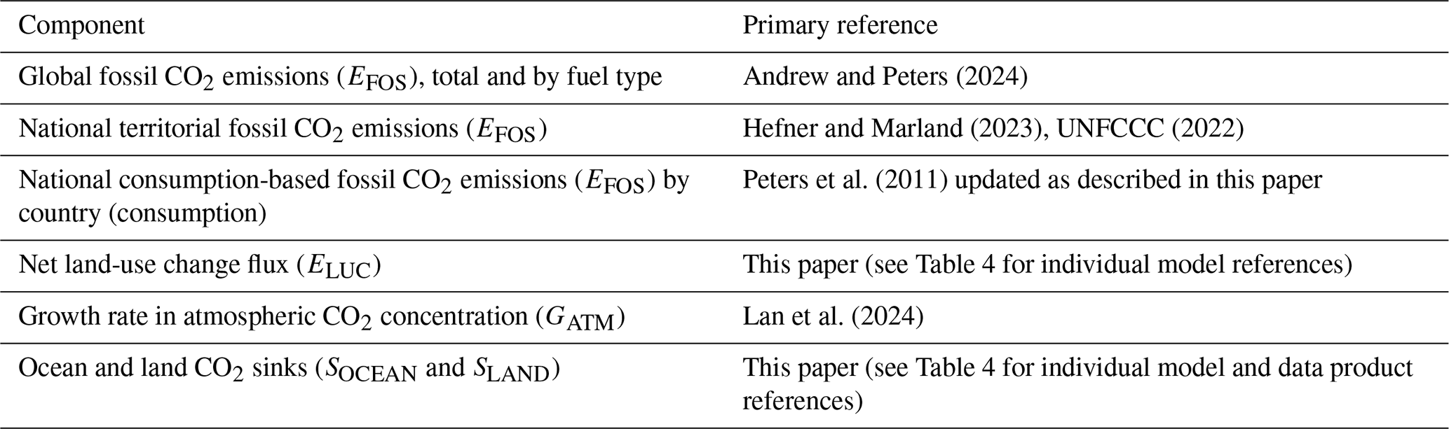
Multiple organizations and research groups around the world have generated the original measurements and data used to complete the global carbon budget. The effort presented here is thus mainly one of synthesis, where results from individual groups are collated, analysed, and evaluated for consistency. We facilitate access to original data with the understanding that primary datasets will be referenced in future work (see Table 2 for how to cite the datasets and the “Data availability” section). Descriptions of the measurements, models, and methodologies follow below, with more detailed descriptions of each component provided in the Supplement (Sects. S1 to S5).

Table 2 How to cite the individual components of the global carbon budget presented here.

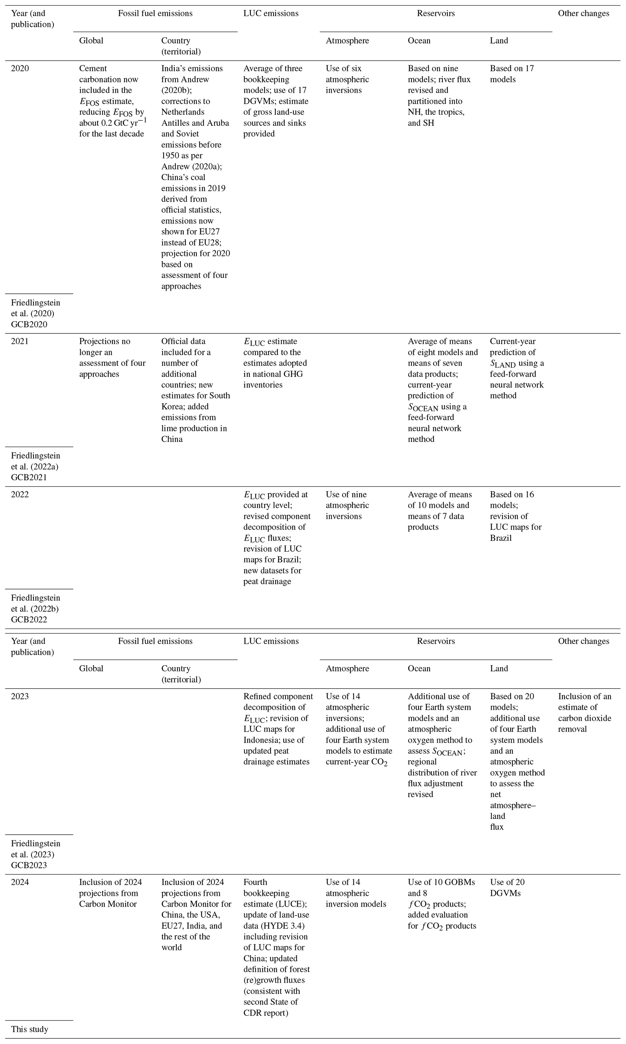
This is the 19th version of the global carbon budget and the 13th revised version in the format of a living-data update in Earth System Science Data. It builds on the latest published global carbon budget of Friedlingstein et al. (2023). The main changes this year are the inclusion of (1) data to the year 2023 and a projection for the global carbon budget for the year 2024 and (2) an estimate of the 2024 projection of fossil emissions from Carbon Monitor. Other methodological differences between recent annual carbon budgets (2020 to 2024) are summarized in Table 3, and previous changes since 2006 are provided in Table S9.

Table 3 The main methodological changes in the global carbon budget since 2020. Methodological changes introduced in one year are kept for the following years unless noted. Empty cells mean there were no methodological changes introduced that year. LUC denotes land-use change; DGVM denotes dynamic global vegetation model; GHG denotes greenhouse gas; NH and SH denote the Northern Hemisphere and Southern Hemisphere, respectively; GOBM denotes global ocean biogeochemistry model. Table S9 lists methodological changes from the first global carbon budget publication up to 2019.

2.1 Fossil CO₂ emissions (E_FOS)

2.1.1 Historical period 1850–2023

The estimates of global and national fossil CO₂ emissions (E_FOS) include the oxidation of fossil fuels through both combustion (e.g. transport, heating) and chemical oxidation (e.g. carbon anode decomposition in aluminium refining) activities and the decomposition of carbonates in industrial processes (e.g. the production of cement). We also include CO₂ uptake from the cement carbonation process. Several emissions sources are not estimated or not fully covered: coverage of emissions from lime production are not global, and decomposition of carbonates in glass and ceramic production is included only for the “Annex I” countries of the United Nations Framework Convention on Climate Change (UNFCCC) for lack of activity data. These omissions are considered to be minor. Short-cycle carbon emissions – for example from combustion of biomass – are not included here but are accounted for in the CO₂ emissions from land use (see Sect. 2.2).

Our estimates of fossil CO₂ emissions rely on data collection by many other parties. Our goal is to produce the best estimate of this flux, and we therefore use a prioritization framework to combine data from different sources that have used different methods while being careful to avoid double counting and undercounting of emissions sources. The CDIAC-FF emissions dataset, derived largely from UN energy data, forms the foundation, and we extend emissions to 2023 using energy growth rates reported by the Energy Institute (a dataset formerly produced by BP). We then proceed to replace estimates using data from what we consider to be superior sources, for example Annex I countries' official submissions to the UNFCCC. All data points, not just those of the latest year, are potentially subject to revision. For full details see Andrew and Peters (2024).

Other estimates of global fossil CO₂ emissions exist, and these are compared by Andrew (2020a). The most common reason for differences in estimates of global fossil CO₂ emissions is a difference in which emissions sources are included in the datasets. Datasets such as those published by the Energy Institute, the US Energy Information Administration, and the International Energy Agency's “CO₂ emissions from fuel combustion” are all generally limited to emissions from combustion of fossil fuels. In contrast, datasets such as PRIMAP-hist, CEDS, EDGAR, and that of GCP aim to include all sources of fossil CO₂ emissions. See Andrew (2020a) for detailed comparisons and discussion.

Cement absorbs CO₂ from the atmosphere over its lifetime, a process known as “cement carbonation”. We estimate this CO₂ sink, from 1931 onwards, as the average of two studies in the literature (Cao et al., 2020; Guo et al., 2021). Both studies use the same model, developed by Xi et al. (2016), with different parameterizations and input data, with the estimate of Guo and colleagues being a revision of that of Xi et al. (2016). The trends of the two studies are very similar. Since carbonation is a function of both current and previous cement production, we extend these estimates to 2023 using the growth rate derived from the smoothed cement emissions (10-year smoothing) fitted to the carbonation data. In the present budget, we always include the cement carbonation carbon sink in the fossil CO₂ emission component (E_FOS).

We use the Kaya identity for a simple decomposition of CO₂ emissions into the key drivers (Raupach et al., 2007). While there are variations (Peters et al., 2017a), we focus here on a decomposition of CO₂ emissions into population, GDP per person, energy use per GDP, and CO₂ emissions per energy unit. Multiplying these individual components together returns the CO₂ emissions. Using the decomposition, it is possible to attribute the change in CO₂ emissions to the change in each of the drivers. This method gives a first-order understanding of what causes CO₂ emissions to change each year.

2.1.2 Year 2024 projection

We provide a projection of global fossil CO₂ emissions in 2024 by combining separate projections for China, the USA, the European Union (EU), India, and all other countries combined. The methods are different for each of these. For China we combine monthly fossil fuel production data from the National Bureau of Statistics and trade data from the customs administration, giving us partial data for the growth rates to date of natural gas, petroleum, and cement and of the apparent consumption itself for raw coal. We then use a regression model to project full-year emissions based on historical observations. For the USA our projection is taken directly from the Energy Information Administration (EIA) Short-Term Energy Outlook (EIA, 2024), combined with the year-to-date growth rate of cement clinker production. For the EU we use monthly energy data from Eurostat to derive estimates of monthly CO₂ emissions, with coal emissions extended using a statistical relationship with reported electricity generation from coal and other factors. For natural gas, preliminary observations are available through December. EU emissions from oil are derived using the EIA's projection of oil consumption for Europe. EU cement emissions are based on available year-to-date data from three of the largest producers, Germany, Poland, and Spain. India's projected emissions are derived from monthly estimates using the methods of Andrew (2020b) and are extrapolated through December assuming seasonal patterns from before 2019. Emissions from international transportation (bunkers) are estimated separately for aviation and shipping. Changes in aviation emissions are derived primarily from Organisation for Economic Co-operation and Development (OECD) monthly estimates, extrapolated using the growth rates of global flight miles from Airportia, and then the final months are projected assuming normal patterns from previous years. Changes in shipping emissions are derived from OECD monthly estimates for global shipping. Emissions for the rest of the world are derived for coal and cement using projected growth in economic production from the IMF (2024) combined with extrapolated changes in emissions intensity of economic production, for oil using a global constraint from the EIA, and for natural gas using a global constraint from the International Energy Agency (IEA). More details on the E_FOS methodology and its 2024 projection can be found in the Supplement, Sect. S1.

For the first time this year, we cross-check our 2024 projection with a 2024 projection from Carbon Monitor. Carbon Monitor is an open-access dataset (https://carbonmonitor.org/, last access: 21 January 2025) of daily emissions constructed using hourly to daily proxy data (e.g. electricity consumption, travel patterns) instead of energy use data. Available Carbon Monitor estimated emissions from January to November are combined into a new projection for December to give a full-year 2024 estimate. The December projections are estimated by leveraging seasonal patterns from 2019–2023 daily CO₂ emissions data from Carbon Monitor. A regression model is applied separately for individual countries to obtain their respective forecast. First, the seasonality component for each month is assessed based on daily average emissions from 2019 to 2023, excluding 2020 due to the COVID-19 pandemic. Then a linear regression model is constructed using the calculated seasonal components and the daily average emissions for the months from January to November 2024. The resulting model is used to project carbon emissions for December 2024. The uncertainty range is calculated using historical monthly variance of seasonal components.

2.2 CO₂ emissions from land-use, land-use change, and forestry (E_LUC)

2.2.1 Historical period 1850–2023

The net CO₂ flux from land-use, land-use change, and forestry (E_LUC, called land-use change emissions in the rest of the text) includes CO₂ fluxes from deforestation, afforestation, logging and forest degradation (including harvest activity), shifting cultivation (cycle of cutting forest for agriculture and then abandoning), regrowth of forests (following wood harvest or agriculture abandonment), peat burning, and peat drainage. Four bookkeeping approaches were used to quantify gross emissions and gross removals and the resulting net E_LUC: the updated estimates for each of BLUE (Hansis et al., 2015), OSCAR (Gasser et al., 2020), and H&C2023 (Houghton and Castanho, 2023) and the new estimates of LUCE (Qin et al., 2024). Emissions from peat burning and peat drainage are added from external datasets (see the Supplement, Sect. S2.1): peat fire emissions from the Global Fire Emissions Database (GFED4.1s; van der Werf et al., 2017) and peat drainage emissions averaged from estimates of the Food and Agriculture Organization (Conchedda and Tubiello, 2020; FAO, 2023a, b) and from simulations with the dynamic global vegetation model (DGVM) ORCHIDEE-PEAT (Qiu et al., 2021) and the DGVM LPX-Bern (Lienert and Joos, 2018; Müller and Joos, 2021). Uncertainty estimates were derived from the DGVM ensemble for the time period prior to 1960, and for the recent decades an uncertainty range of ±0.7 GtC yr⁻¹ was used, which is a semi-quantitative measure for annual and decadal emissions and reflects our best value judgement that there is at least a 68 % chance (±1σ) that the true land-use change emission lies within the given range for the range of processes considered here.

The GCB E_LUC estimates follow the CO₂ flux definition of global carbon cycle models and differ from IPCC definitions adopted in national greenhouse gas inventories (NGHGIs) for reporting under the UNFCCC. The latter typically include terrestrial fluxes occurring on all land that countries define as managed, following the IPCC managed-land proxy approach (Grassi et al., 2018). This partly includes fluxes due to environmental change (e.g. atmospheric CO₂ increase), which are part of S_LAND in our definition. As a result, global emissions estimates are smaller for NGHGIs than for the global carbon budget definition (Grassi et al., 2023). The same is the case for the FAO estimates of carbon fluxes on forest land, which include both anthropogenic and natural fluxes on managed land (Tubiello et al., 2021). We map the GCB and NGHGI definitions onto each other to provide a comparison of the anthropogenic carbon budget as reported in the GCB to the official country reporting to the UNFCCC convention. We further compare these estimates with the net atmosphere-to-land flux from atmospheric inversion systems (see Sect. 2.7), averaged over managed land only.

E_LUC contains a range of fluxes that are related to carbon dioxide removal (CDR). CDR is defined as the set of anthropogenic activities that remove CO₂ from the atmosphere, in addition to the Earth's natural processes (such as carbon uptake in response to atmospheric CO₂ increase), and store it in durable form, such as in forest biomass, soils, long-lived products, the ocean, or geological reservoirs. Here, we quantify vegetation-based CDR that is implicitly or explicitly captured by land-use fluxes (CDR not based on vegetation is discussed in Sect. 2.3). We quantify re-/afforestation from the four bookkeeping estimates by separating forest regrowth into shifting cultivation cycles from permanent increases in forest cover (see the Supplement, Sect. S2.1). The latter count as CDR, but it should be noted that the permanence of the storage under climate risks such as fire is increasingly questioned. Other CDR activities related to land use but not fully accounted for in our E_LUC estimate include the transfer of carbon to harvested wood products (HWPs), bioenergy with carbon capture and storage (BECCS), and biochar production (Babiker et al., 2022; Smith et al., 2024). The different bookkeeping models all represent HWPs but with varying details concerning product usage and their lifetimes. BECCS and biochar are currently only represented in bookkeeping and TRENDY models with regard to the CO₂ removal through photosynthesis, without accounting for the durable storage. HWPs, BECCS, and biochar are typically counted as CDR once the transfer to the durable storage site occurs and not when the CO₂ is removed from the atmosphere, which complicates a direct comparison to the GCB approach to quantify annual fluxes to and from the atmosphere. We provide estimates for CDR through HWPs, BECCS, and biochar based on independent studies in Sect. 3.2.2, but we do not add them to our E_LUC estimate to avoid potential double counting that arises from the partial consideration of HWPs, BECCS, and biochar in the bookkeeping and TRENDY models and to avoid inconsistencies from the temporal discrepancy between transfer to storage and removal from the atmosphere.

2.2.2 Year 2024 projection

We project the 2024 land-use emissions for BLUE, H&C2023, OSCAR, and LUCE based on their E_LUC estimates for 2023 and on adding the change in carbon emissions from peat fires and tropical deforestation and degradation fires (2024 emissions relative to 2023 emissions) estimated using active fire data (MCD14ML; Giglio et al., 2016). Peat drainage is assumed to be unaltered as it has low interannual variability. More details on the E_LUC methodology can be found in the Supplement, Sect. S2.

2.3 Carbon dioxide removal (CDR) not based on vegetation

While some CDR involves CO₂ fluxes via land use and is included in our estimate of E_LUC (re-/afforestation) or provided from other data sources (biochar, HWPs, and BECCS), other CDR occurs through fluxes of CO₂ directly from the air to the geosphere. The majority of this derives from enhanced weathering through the application of crushed rock to soils, with a smaller contribution from direct air carbon capture and storage (DACCS). We use data from the State of CDR report (Smith et al., 2024), which compiles and harmonizes reported removal rates from a combination of existing databases, surveys, and novel research. Currently there are no internationally agreed methods for reporting these CDR types, meaning estimates are based on self-disclosure by projects following their own protocols. As such, the fractional uncertainty in these numbers should be viewed as substantial, and they are liable to change in future years as protocols are harmonized and improved.

2.4 Growth rate in atmospheric CO₂ concentration (G_ATM)

2.4.1 Historical period 1850–2023

The rate of growth of the atmospheric CO₂ concentration is provided for the years 1959–2023 by the US National Oceanic and Atmospheric Administration Global Monitoring Laboratory (NOAA/GML; Lan et al., 2024), which includes recent revisions to the calibration scale of atmospheric CO₂ measurements (WMO CO₂ X2019; Hall et al., 2021). For the 1959–1979 period, the global growth rate is based on measurements of atmospheric CO₂ concentration averaged from the Mauna Loa and South Pole stations, as observed by the CO₂ Program at Scripps Institution of Oceanography (Keeling et al., 1976). For the 1980–2021 time period, the global growth rate is based on the average of multiple stations selected from the marine boundary layer sites with well-mixed background air (Lan et al., 2023) after fitting a smooth curve through the data for each station as a function of time and averaging by latitude band (Masarie and Tans, 1995). The annual growth rate is estimated by Lan et al. (2024) from atmospheric CO₂ concentration by taking the average of the most recent December–January months corrected for the average seasonal cycle and subtracting this same average 1 year earlier. The growth rate in units of ppm yr⁻¹ is converted to units of GtC yr⁻¹ by multiplying by a factor of 2.124 GtC ppm⁻¹, assuming instantaneous mixing of CO₂ throughout the atmosphere (Ballantyne et al., 2012; Table 1).

The uncertainty around the atmospheric growth rate is due to three main factors. The first uncertainty is related to the network composition of the marine boundary layer sites with some sites coming or going, gaps in the time series at each site, etc. This uncertainty was estimated with a bootstrap method by constructing 100 “alternative” networks (Steele et al., 1992; Masarie and Tans, 1995; Lan et al., 2024). The second uncertainty is the analytical uncertainty that describes the short- and long-term uncertainties associated with the CO₂ analysers. A Monte Carlo method was used to estimate the total analytical uncertainty by randomly selecting errors to add to each observation from a normal distribution of combined short- and long-term uncertainties. Prior to the 1980s when analysers were less precise and the CO₂ measurement scale was slightly less well defined, larger analytical errors were assigned to account for these factors. However, the network uncertainty remains the larger term of uncertainty. The first and second uncertainties are reported as 1σ standard deviations (i.e. 68 % confidence interval) and are summed in quadrature to determine the global surface growth rate uncertainty, which averaged to 0.085 ppm. The third uncertainty is the uncertainty associated with using the average CO₂ concentration from a surface network to approximate the true atmospheric average CO₂ concentration (mass-weighted, in three dimensions) as needed to assess the total atmospheric CO₂ burden. In reality, CO₂ variations measured at the stations will not exactly track the changes in total atmospheric burden, with offsets in magnitude and phasing due to vertical and horizontal mixing. This effect must be very small on decadal and longer timescales, when the atmosphere can be considered well mixed. The long-term CO₂ increase in the stratosphere lags the increase (meaning lower concentrations) that we observe in the marine boundary layer, while the continental boundary layer (where most of the emissions take place) leads the marine boundary layer with higher concentrations. These effects nearly cancel each other out. In addition, the growth rate is nearly the same everywhere (Ballantyne et al., 2012). We therefore maintain an uncertainty around the annual growth rate based on the multiple-station dataset ranges between 0.11 and 0.72 GtC yr⁻¹, with a mean of 0.61 GtC yr⁻¹ for 1959–1979 and 0.17 GtC yr⁻¹ for 1980–2023, when more measurement sites were available (Lan et al., 2024). We estimate the uncertainty in the decadally averaged growth rate after 1980 at 0.02 GtC yr⁻¹ based on the annual growth rate uncertainty but stretched over a 10-year interval. For years prior to 1980, we estimate the decadally averaged uncertainty to be 0.07 GtC yr⁻¹ based on a factor proportional to the annual uncertainty prior to and after 1980 ($\mathrm{0.02}\times (\mathrm{0.61}/\mathrm{0.17})$ GtC yr⁻¹).

We assign a high confidence to the annual estimates of G_ATM because they are based on direct measurements from stations distributed around the world (Lan et al., 2023) with all CO₂ measurements consistently measured against the same CO₂ standard scale (WMO CO₂ X2019) defined by a suite of gas standards (Hall et al., 2021).

To estimate the total carbon accumulated in the atmosphere since 1750 and 1850, we use an atmospheric CO₂ concentration of 278.3 ± 3 ppm and 285.1 ± 3 ppm, respectively (Gulev et al., 2021). For the construction of the cumulative budget shown in Fig. 3, we use the fitted estimates of CO₂ concentration from Joos and Spahni (2008) and the conversion factors shown in Table 1 to estimate the annual atmospheric growth rate. The uncertainty of ±3 ppm (converted into ±1σ) is taken directly from the IPCC's AR5 (Ciais et al., 2013). Typical uncertainties in the growth rate in atmospheric CO₂ concentration from ice core data are equivalent to ±0.1–0.15 GtC yr⁻¹, as evaluated from the Law Dome data (Etheridge et al., 1996) for individual 20-year intervals over the period from 1850 to 1960 (Bruno and Joos, 1997).

2.4.2 Year 2024 projection

We provide an assessment of G_ATM for 2024 as the average of two methods. The GCB regression method models monthly global-average atmospheric CO₂ concentrations and derives the increment and annual average from these. The model uses lagged observations of concentration (Lan et al., 2024): both a 12-month lag and the lowest lag that will allow the model prediction to produce an estimate for the following January, recalling that the G_ATM increment is derived from December–January pairs. The largest driver of interannual changes is the El Niño–Southern Oscillation (ENSO) signal (Betts et al., 2016), so the monthly Niño 3.4 index (Huang et al., 2017) is included in the model. Given the natural lag between sea-surface temperatures and effects on the biosphere and in turn effects on globally mixed atmospheric CO₂ concentration, a lagged ENSO index is used, and we use both a 5-month and a 6-month lag. The combination of the two lagged ENSO values helps reduce possible effects of noise in a single month. To help characterize the seasonal variation, we add “month” as a categorical variable. Finally, we flag the period affected by the Pinatubo eruption (August 1991–November 1993) as a categorical variable. Note that while emissions of CO₂ are the largest driver of the trend in atmospheric CO₂ concentration, our goal here is to predict divergence from that trend. Because changes in emissions from year to year are relatively minor in comparison to total emissions, this has little effect on the variation in concentration from the trend line. Even the relatively large drop in emissions in 2020 due to the COVID-19 pandemic does not cause any problems for the model.

We also use the multi-model mean and uncertainty in the 2024 G_ATM estimated by the ESM prediction system (see Sect. 2.9). We then take the average of the GCB regression and ESM G_ATM estimates, with their respective uncertainty combined quadratically.

Similarly, the projection of the 2024 global-average CO₂ concentration (in ppm) is calculated as the average of the estimates from the two methods. For the GCB regression method, it is the annual average of global concentration over the 12 months of 2024; for the ESMs, it is the observed global-average CO₂ concentration for 2023 and the annual increase in 2024 of the global-average CO₂ concentration predicted by the ESM multi-model mean.

2.5 Ocean CO₂ sink

2.5.1 Historical period 1850–2023

The reported estimate of the global ocean anthropogenic CO₂ sink S_OCEAN is derived as the average of two estimates. The first estimate is derived as the mean over an ensemble of 10 global ocean biogeochemistry models (GOBMs; Tables 4 and S2). The second estimate is obtained as the mean over an ensemble of eight surface ocean fCO₂ observation-based data products (fCO₂ is the fugacity of CO₂; Tables 4 and S3). A ninth fCO₂ product (UExP-FFN-U) is shown but is not included in the ensemble average as it differs from the other products by adjusting the flux to a cool, salty ocean surface skin. In previous editions of the GCB, this product was obtained following the Watson et al. (2020) method, but it has been updated following the method of Dong et al. (2022; see the Supplement, Sect. S3.1, for a discussion). The GOBMs simulate both the natural and the anthropogenic CO₂ cycles in the ocean. They constrain the anthropogenic air–sea CO₂ flux (the dominant component of S_OCEAN) by the transport of carbon into the ocean interior, which is also the controlling factor of present-day ocean carbon uptake in the real world. They cover the full globe and all seasons and were evaluated against surface ocean carbon observations, suggesting they are suitable for estimating the annual ocean carbon sink (Hauck et al., 2020). The fCO₂ products are tightly linked to observations of fCO₂ (fugacity of CO₂, which equals pCO₂ corrected for the non-ideal behaviour of the gas; Pfeil et al., 2013), which carry imprints of temporal and spatial variability but are also sensitive to uncertainties in gas-exchange parameterizations and data sparsity (Fay et al., 2021; Gloege et al., 2021; Hauck et al., 2023a). Their advantage is the assessment of the mean spatial pattern of variability and its seasonality (Hauck et al., 2020; Gloege et al., 2021; Hauck et al., 2023a). To benchmark trends derived from the fCO₂ products, we additionally performed a model subsampling exercise following Hauck et al. (2023a; see Sect. S3). In addition, two diagnostic ocean models are used to estimate S_OCEAN over the industrial era (1781–1958).

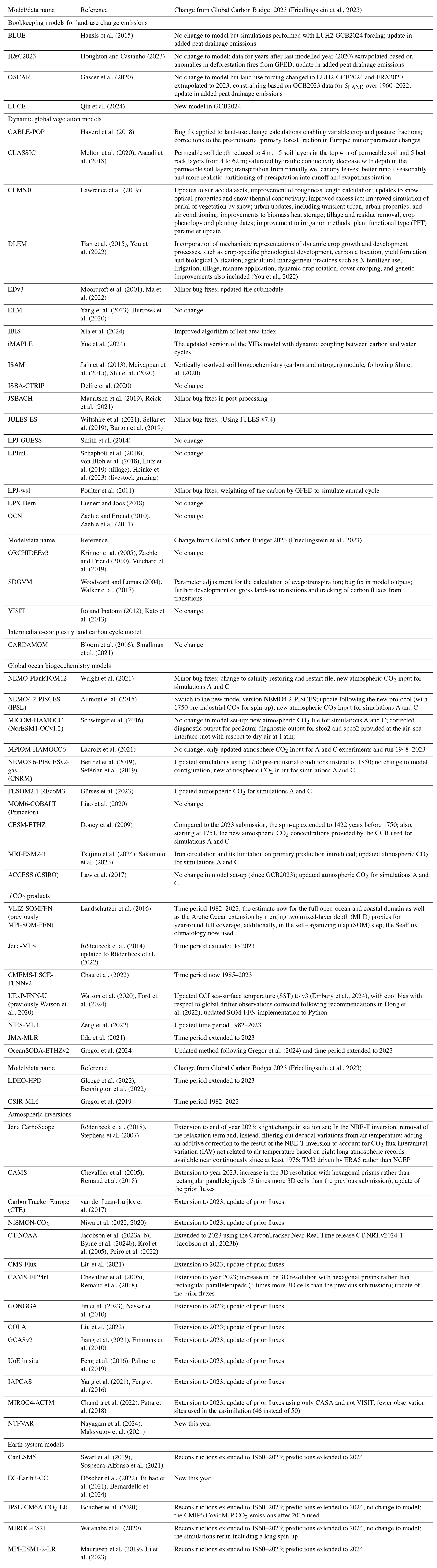
Table 4 References for the process models, bookkeeping models, ocean data products, and atmospheric inversions. All models and products are updated with new data to the end of the year 2023.

The global fCO₂-based flux estimates were adjusted to remove the pre-industrial ocean source of CO₂ to the atmosphere of 0.65 ± 0.3 GtC yr⁻¹ from river input to the ocean (Regnier et al., 2022) in order to satisfy our definition of S_OCEAN (Hauck et al., 2020). The river flux adjustment was distributed over the latitudinal bands using the regional distribution of Lacroix et al. (2020; north: 0.14 GtC yr⁻¹; tropics: 0.42 GtC yr⁻¹; south: 0.09 GtC yr⁻¹). Acknowledging that this distribution is based on only one model, the advantage is that a gridded field is available, and the river flux adjustment can be calculated for the three latitudinal bands and the RECCAP (REgional Carbon Cycle Assessment and Processes) regions (RECCAP-2; Ciais et al., 2022; Poulter et al., 2022; DeVries et al., 2023). This dataset suggests that more of the riverine outgassing is located in the tropics than in the Southern Ocean and is thus opposed to the previously used dataset of Aumont et al. (2001). Accordingly, the regional distribution is associated with a major uncertainty in addition to the large uncertainty around the global estimate (Crisp et al., 2022; Gruber et al., 2023). Anthropogenic perturbations of river carbon and nutrient transport to the ocean are not considered (see Sects. 2.10 and S6.3).

We derive S_OCEAN from GOBMs using a simulation (sim A) with historical forcing of climate and atmospheric CO₂ from the GCB (Sect. 2.4), accounting for model biases and drift from a control simulation (sim B) with constant atmospheric CO₂ and normal-year climate forcing. A third simulation (sim C) with historical atmospheric CO₂ increase and normal-year climate forcing is used to attribute the ocean sink to CO₂ (sim C minus sim B) and climate (sim A minus sim C) effects. A fourth simulation (sim D; historical climate forcing and constant atmospheric CO₂) is used to compare the change in the anthropogenic carbon inventory in the interior ocean (sim A minus sim D) to the observational estimate of Gruber et al. (2019) with the same flux components (steady-state and non-steady-state anthropogenic carbon flux). The fCO₂ products are adjusted with respect to their original publications to represent the full ice-free ocean area, including coastal zones and marginal seas, when the area coverage is below 99 %. This is done by either area filling following Fay et al. (2021) or a simple scaling approach. GOBMs and fCO₂ products fall within the observational constraints over the 1990s (2.2 ± 0.7 GtC yr⁻¹; Ciais et al., 2013) before and after applying adjustments.

S_OCEAN is calculated as the average of the GOBM ensemble mean and the fCO₂-product ensemble mean from 1990 onwards. Prior to 1990, it is calculated as the GOBM ensemble mean and half of the offset between GOBM and fCO₂-product ensemble means over 1990–2001.

We assign an uncertainty of ±0.4 GtC yr⁻¹ to the ocean sink based on a combination of random (ensemble standard deviation) and systematic uncertainties (GOBM bias in anthropogenic carbon accumulation, previously reported uncertainties in fCO₂ products; see the Supplement, Sect. S3.4). While this approach is consistent within the GCB, an independent uncertainty assessment of the fCO₂ products alone suggests a somewhat larger uncertainty of up to 0.7 GtC yr⁻¹ (Ford et al., 2024). We assign a medium confidence level to the annual ocean CO₂ sink and its uncertainty because it is based on multiple lines of evidence, it is consistent with ocean interior carbon estimates (Gruber et al., 2019; see Sect. 3.6.5), and the interannual variability in the GOBMs and data-based estimates is largely consistent and can be explained by climate variability. We refrain from assigning a high confidence level because of the deviation between the GOBM and fCO₂-product trends between around 2002 and 2020. More details on the S_OCEAN methodology can be found in the Supplement, Sect. S3.

2.5.2 Year 2024 projection

The ocean CO₂ sink forecast for the year 2024 is based on (a) the historical (Lan et al., 2024) and our 2024 estimate of atmospheric CO₂ concentration, (b) the historical and our 2024 estimate of global fossil fuel emissions, and (c) the boreal spring (March, April, May) Oceanic Niño Index (ONI) (NCEP, 2024). Using a non-linear regression approach, i.e. a feed-forward neural network, atmospheric CO₂, ONI, and the fossil fuel emissions are used as training data to best match the annual ocean CO₂ sink (i.e. combined S_OCEAN estimate from GOBMs and data products) from 1959 through 2023 from this year's carbon budget. Using this relationship, the 2024 S_OCEAN can then be estimated from the projected 2024 input data using the non-linear relationship established during the network training. To avoid overfitting, the neural network training was done using a Monte Carlo approach, with a variable number of artificial neurons (varying between two and five), and 20 % of the randomly selected training data were withheld for independent internal testing.

Based on the best output performance (tested using the 20 % withheld input data), the best-performing number of neurons was selected. In a second step, we trained the network 10 times using the best number of neurons identified in step 1 and different sets of randomly selected training data. The mean of the 10 training runs is considered our best forecast, whereas the standard deviation of the 10 ensembles provides a first-order estimate of the forecast uncertainty. This uncertainty is then combined with the S_OCEAN uncertainty (0.4 GtC yr⁻¹) to estimate the overall uncertainty in the 2024 projection. As an additional line of evidence, we also assess the 2024 atmosphere–ocean carbon flux from the ESM prediction system (see Sect. 2.9).

2.6 Land CO₂ sink

2.6.1 Historical period 1850–2023

The terrestrial land sink (S_LAND) is thought to be due to the combined effects of rising atmospheric CO₂, increasing N inputs, and climate change on plant growth and terrestrial carbon storage. S_LAND does not include land sinks directly resulting from land-use and land-use change (e.g. regrowth of vegetation) as these are part of the land-use flux (E_LUC), although system boundaries make it difficult to exactly attribute CO₂ fluxes on land to S_LAND and E_LUC (Erb et al., 2013).

S_LAND is estimated from the multi-model mean of 20 DGVMs (Tables 4 and S1). DGVM simulations include all climate variability and CO₂ effects over land. In addition to the carbon cycle represented in all DGVMs, 14 models also account for the nitrogen cycle and hence can include the effect of N inputs on S_LAND. The DGVM estimate of S_LAND does not include the export of carbon to aquatic systems or its historical perturbation, which is discussed in the Supplement, Sect. S6.3. DGVMs need to meet several criteria to be included in this assessment. In addition, we use the International Land Model Benchmarking (ILAMB) system (Collier et al., 2018) for the DGVM evaluation (see the Supplement, Sect. S4.2), with an additional comparison of DGVMs with a data-informed Bayesian model–data fusion framework (CARDAMOM) (Bloom and Williams, 2015; Bloom et al., 2016). The uncertainty in S_LAND is taken from the DGVM standard deviation. More details on the S_LAND methodology can be found in the Supplement, Sect. S4.

2.6.2 Year 2024 projection

Like for the ocean forecast, the land CO₂ sink forecast for the year 2024 is based on (a) the historical (Lan et al., 2024) and our 2024 estimate of atmospheric CO₂ concentration, (b) the historical and our 2024 estimate of global fossil fuel emissions, and (c) the boreal summer (June, July, August) Oceanic Niño Index (ONI) (NCEP, 2024). All training data are again used to best match S_LAND from 1959 through 2023 from this year's carbon budget using a feed-forward neural network. To avoid overfitting, the neural network was trained with a variable number of artificial neurons (varying between 2–15), larger than for S_OCEAN prediction due to the stronger land carbon interannual variability. As done for S_OCEAN, Monte Carlo-type pre-training selects the optimal number of artificial neurons based on 20 % withheld input data, and in a second step, an ensemble of 10 forecasts is produced to provide the mean forecast and uncertainty. This uncertainty is then combined with the S_LAND uncertainty for 2023 (1.0 GtC yr⁻¹) to estimate the overall uncertainty in the 2024 projection.

2.7 Atmospheric inversion estimate

The worldwide network of in situ atmospheric measurements and satellite-derived atmospheric CO₂ column (XCO₂) observations put a strong constraint on changes in the atmospheric abundance of CO₂. This is true not only globally (hence our large confidence in G_ATM), but also in regions with sufficient observational density, found mostly in the extra-tropics. This allows atmospheric inversion methods to constrain the magnitude and location of the combined total surface CO₂ fluxes from all sources, including fossil and land-use change emissions and land and ocean CO₂ fluxes. The inversions assume E_FOS to be well known, and they solve for the spatial and temporal distribution of land and ocean fluxes from the residual gradients of CO₂ between stations that are not explained by fossil fuel emissions. By design, such systems thus close the carbon balance (B_IM=0) and provide an additional perspective on the independent estimates of the ocean and land fluxes.

This year's release includes 14 inversion systems that are described in Table S4. Each system is rooted in Bayesian inversion principles but uses different methodologies. These differences concern the selection of atmospheric CO₂ data or XCO₂ and the choice of a priori fluxes to refine. They also differ in spatial and temporal resolution, assumed correlation structures, and the mathematical approach of their models (see references in Table S4 for details). Importantly, the systems use a variety of transport models, which was demonstrated to be a driving factor behind differences in atmospheric-inversion-based flux estimates and specifically their distribution across latitudinal bands (Gaubert et al., 2019; Schuh et al., 2019). Eight inversion systems used surface observations from the global measurement network (Schuldt et al., 2023, 2024). Six inversion systems (CAMS-FT24r1, CMS-Flux, GONGGA, COLA, GCASv2, NTFVAR) used satellite XCO₂ retrievals from GOSAT and/or OCO-2, scaled to the WMO CO₂ X2019 calibration scale, and this year three of these inversion systems (CMS-Flux, COLA, NTFVAR) used these XCO₂ datasets in addition to the in situ observational CO₂ mole fraction records.

The original products delivered by the inverse modellers were modified to facilitate comparison to the other elements of the budget, specifically on two accounts: (1) global total fossil fuel emissions including cement carbonation CO₂ uptake and (2) riverine CO₂ transport. We note that with these adjustments, the inverse results no longer represent the net atmosphere–surface exchange over land and ocean areas as sensed by atmospheric observations. Instead, for land, they become the net uptake of CO₂ by vegetation and soils that is not exported by fluvial systems, which is similar to the DGVM estimates. For oceans, they become the net uptake of anthropogenic CO₂, which similar to the GOBM estimates.

The inversion systems prescribe global fossil fuel emissions based on, for example, the GCP's Gridded Fossil Emissions Dataset version 2024.0 (GCP-GridFED; Jones et al., 2024a), which is an update to GCP-GridFEDv2021 presented by Jones et al. (2021b). GCP-GridFEDv2024.0 scales gridded estimates of CO₂ emissions from EDGAR v4.3.2 (Janssens-Maenhout et al., 2019) within national territories to match national emissions estimates provided by the GCB for the years 1959–2023, which were compiled following the methodology described in Sect. 2.1. Small differences between the systems due to, for instance, regridding to the transport model resolution or use of fossil fuel emissions that are different to those of GCP-GridFEDv2024.0 are adjusted in the latitudinal partitioning we present to ensure agreement with the estimate of E_FOS in this budget. We also note that the ocean fluxes used as prior by 8 out of 14 inversions are part of the suite of the ocean process model or fCO₂ products listed in Sect. 2.5. Although these fluxes are further adjusted by the atmospheric inversions (except for Jena CarboScope), it means the inversion estimates of the ocean fluxes are not completely independent of S_OCEAN assessed here.

To facilitate comparisons to the independent S_OCEAN and S_LAND values, we used the same adjustments for transport and outgassing of carbon transported from land to ocean, as done for the observation-based estimates of S_OCEAN (see the Supplement, Sect. S3).

The atmospheric inversions are evaluated using vertical profiles of atmospheric CO₂ concentrations (Fig. S5). More than 30 aircraft programmes over the globe, either regular programmes or repeated surveys over at least 9 months (except for SH programmes), have been used to assess system performance (with space–time observational coverage sparse in the SH and tropics and denser in NH mid-latitudes; Table S8). The 14 systems are compared to the independent aircraft CO₂ measurements between 2 and 7 km above sea level between 2001 and 2023. Results are shown in Fig. S5 and discussed in the Supplement, Sect. S5.2.

With a relatively small ensemble of systems that cover at least 1 full decade (N=10) and which moreover share some a priori fluxes used with one another or with the process-based models, it is difficult to justify using their mean and standard deviation as metrics for uncertainty across the ensemble. We therefore report their full range (min–max) without their mean. More details on the atmospheric inversion methodology can be found in the Supplement, Sect. S5.

2.8 Atmospheric-oxygen-based estimate

Long-term atmospheric O₂ and CO₂ observations allow estimation of the global ocean and land carbon sinks due to the coupling of O₂ and CO₂ with distinct exchange ratios for fossil fuel emissions and land uptake and uncoupled O₂ and CO₂ ocean exchange (Keeling and Manning, 2014). The global ocean and net land carbon sinks were calculated following methods and constants used in Keeling and Manning (2014) but were modified to also include the effective O₂ source from metal refining (Battle et al., 2023). For the exchange ratio of the net land sink, a value of 1.05 is used, following Resplandy et al. (2019). For fossil fuels, the following values are used: gas, 1.95 ± 0.04; liquid, 1.44 ± 0.03; solid, 1.17 ± 0.03; cement, 0 ± 0; and gas flaring, 1.98 ± 0.07 (Keeling, 1988). Atmospheric O₂ is observed as δ(${\mathrm{O}}_{\mathrm{2}}/{\mathrm{N}}_{\mathrm{2}}$) and combined with CO₂ mole fraction observations into atmospheric potential oxygen (APO; Stephens et al., 1998). The APO observations from 1990 to 2024 were taken from a weighted average of flask records from three stations in the Scripps O₂ Program network (Alert, Canada (ALT); La Jolla, California (LJO); and Cape Grim, Australia (CGO), weighted as per Keeling and Manning (2014). Observed CO₂ was taken from the globally averaged marine surface annual mean growth rate from the NOAA/GML Global Greenhouse Gas Reference Network (Lan et al., 2024). The O₂ source from ocean warming is based on ocean heat content from updated data from NOAA/NCEI (Levitus et al., 2012). The effective O₂ source from metal refining is based on production data from Bray (2020), Flanagan (2021), and Tuck (2022). Uncertainty was determined through a Monte Carlo approach with 20 000 iterations, using uncertainties prescribed in Keeling and Manning (2014), including observational uncertainties from Keeling et al. (2007) and autoregressive errors in fossil fuel emissions (Ballantyne et al., 2015). The reported uncertainty is 1 standard deviation of the ensemble. The difference from the atmospheric O₂ estimate for GCB2023 is due to a revision to the Scripps O₂ Program CO₂ data. As with the atmospheric inversions, the O₂-based estimates also close the carbon balance (B_IM=0) by design and provide another independent estimate of the ocean and land fluxes. Note that the O₂ method requires a correction for global air–sea O₂ flux; this has the largest uncertainty at annual timescales but which is still non-negligible for decadal estimates (Nevison et al., 2008).

2.9 Earth system models' estimate

Reconstructions and predictions from decadal prediction systems based on Earth system models (ESMs) provide a novel line of evidence in assessing the atmosphere–land and atmosphere–ocean carbon fluxes in the past decades and predicting their changes for the current year. The decadal prediction systems based on ESMs used here consist of three sets of simulations: (i) uninitialized freely evolving historical simulations (1850–2014); (ii) assimilation reconstruction incorporating observational data into the model (1960–2023); and (iii) initialized prediction simulations for the 1981–2024 period, starting every year from initial states obtained from the above assimilation simulations. The assimilations are designed to reconstruct the actual evolution of the Earth system by assimilating essential fields from data products. The assimilations' states, which are expected to be close to observations, are used to start the initialized prediction simulations used for the current-year (2024) global carbon budget. Similar initialized prediction simulations starting every year (1 November or 1 January) over the 1981–2023 period (i.e. hindcasts) are also performed for predictive skill quantification and for bias correction. More details on the illustration of a decadal prediction system based on an ESM can be found in Fig. 1 of Li et al. (2023).

By assimilating physical atmospheric and oceanic data products into the ESMs, the models are able to reproduce the historical variations in the atmosphere–sea CO₂ fluxes, atmosphere–land CO₂ fluxes, and atmospheric CO₂ growth rate (Li et al., 2016, 2019; Lovenduski et al., 2019a, b; Ilyina et al., 2021; Li et al., 2023). Furthermore, the ESM-based predictions have proven their skill in predicting the air–sea CO₂ fluxes for up to 6 years and the air–land CO₂ fluxes and atmospheric CO₂ growth for 2 years (Lovenduski et al., 2019a, b; Ilyina et al., 2021; Li et al., 2023). The reconstructions from the fully coupled model simulations ensure a closed budget within the Earth system, i.e. no budget imbalance term.

Five ESMs, i.e. CanESM5 (Swart et al., 2019; Sospedra-Alfonso et al., 2021), EC-Earth3-CC (Döscher et al., 2022; Bilbao et al., 2021; Bernardello et al., 2024), IPSL-CM6A-CO₂-LR (Boucher et al., 2020), MIROC-ES2L (Watanabe et al., 2020), and MPI-ESM1-2-LR (Mauritsen et al., 2019; Li et al., 2023), have performed the set of prediction simulations. Each ESM uses a different assimilation method and combination of data products incorporated in the system; more details on the models' configuration can be found in Tables 4 and S5. The ESMs use external forcings from the Coupled Model Intercomparison Project Phase 6 (CMIP6) historical (1960–2014) and SSP2-4.5 baseline and CovidMIP 2-year blip scenarios (2015–2024) (Eyring et al., 2016; Lamboll et al., 2021). The CO₂ emissions forcing from 2015–2024 is substituted by GCB-GridFED (v2024.0, Jones et al., 2024a) to provide a consistent CO₂ forcing. Reconstructions of atmosphere–ocean CO₂ fluxes (S_OCEAN) and atmosphere–land CO₂ fluxes (S_LAND−E_LUC) for the time period from 1960–2023 are assessed here. Predictions of the atmosphere–ocean CO₂ flux, atmosphere–land CO₂ flux, and atmospheric CO₂ growth for 2024 are calculated based on the predictions at a lead time of 1 year. The predictions are bias-corrected using the 1985–2014 climatology mean of GCB2022 (Friedlingstein et al., 2022b); more details on methods can be found in Boer et al. (2016) and Li et al. (2023). The ensemble size of initialized prediction simulations is 10, and the ensemble mean for each individual model is used here. The ESMs are used here to support the assessment of S_OCEAN and net atmosphere–land CO₂ flux (S_LAND−E_LUC) over the 1960–2023 period and to provide an estimate of the 2024 projection of G_ATM.

2.10 Processes not included in the global carbon budget

The contribution of anthropogenic CO and CH₄ to the global carbon budget is not fully accounted for in Eq. (1) and is described in the Supplement, Sect. S6.1. The contributions to CO₂ emissions of the decomposition of carbonates not accounted for are described in the Supplement, Sect. S6.2. The contribution of anthropogenic changes in river fluxes is conceptually included in Eq. (1) in S_OCEAN and in S_LAND, but it is not represented in the process models used to quantify these fluxes. This effect is discussed in the Supplement, Sect. S6.3. Similarly, the loss of additional sink capacity from reduced forest cover is missing in the combination of approaches used here to estimate both land fluxes (E_LUC and S_LAND), and its potential effect is discussed and quantified in the Supplement, Sect. S6.4.

3 Results

For each component of the global carbon budget, we present results for three different time periods: the full historical period, from 1850 to 2023, the decades for which we have atmospheric concentration records from Mauna Loa (1960–2023); a specific focus on last year (2023); and the projection for the current year (2024). Subsequently, we assess the estimates of the budget components of recent decades against the top-down constraints from inverse modelling of atmospheric observations, the land–ocean partitioning derived from the atmospheric O₂ measurements, and the budget component estimates from the ESM assimilation simulations. Atmospheric inversions further allow for an assessment of the budget components with a regional breakdown of land and ocean sinks.

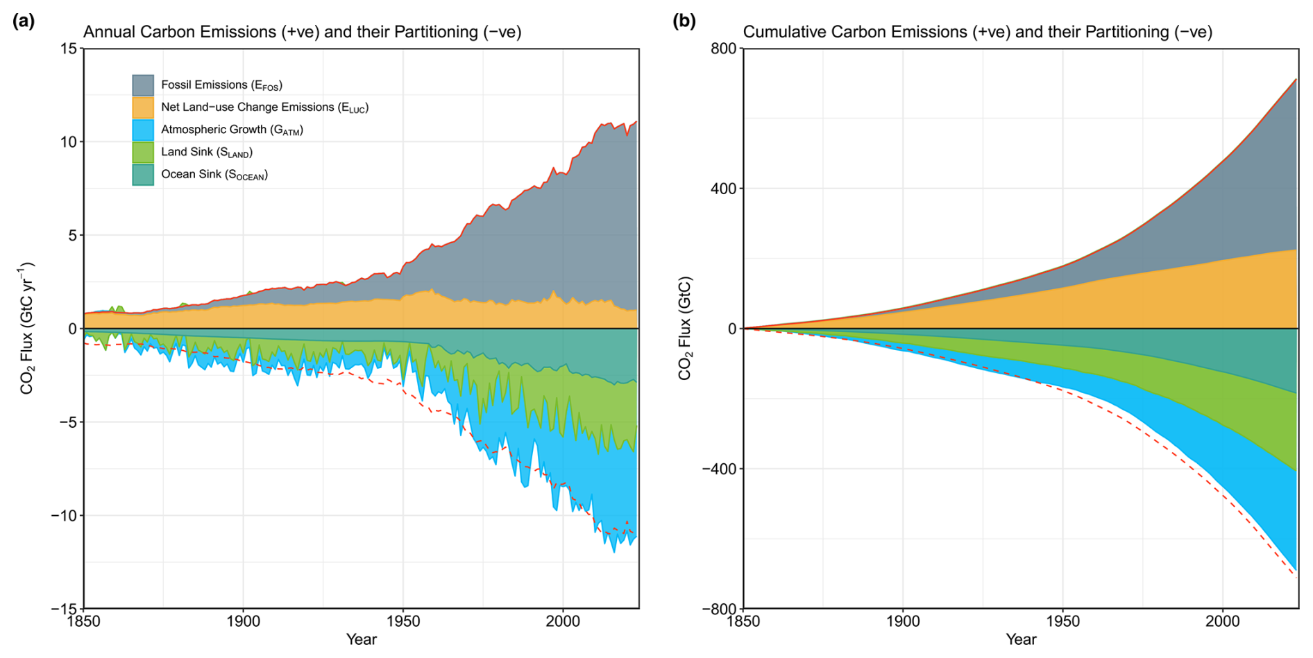
Figure 3 Combined components of the global carbon budget as a function of time, for fossil CO₂ emissions (E_FOS, including a small sink from cement carbonation; grey) and emissions from land-use change (E_LUC; yellow-brown), as well as their partitioning into the atmosphere (G_ATM; cyan), ocean (S_OCEAN; turquoise), and land (S_LAND; green). Panel (a) shows annual estimates of each flux (in GtC yr⁻¹) and panel (b) the cumulative flux (the sum of all prior annual fluxes, in GtC) since the year 1850. The partitioning is based on nearly independent estimates from observations (for G_ATM) and from process model ensembles constrained by data (for S_OCEAN and S_LAND) and does not exactly add up to the sum of the emissions, resulting in a budget imbalance (B_IM) which is represented by the difference between the bottom red line (mirroring total emissions) and the sum of carbon fluxes in the ocean, land, and atmosphere reservoirs. All data are in gigatonnes of carbon per year (GtC yr⁻¹) (a) and gigatonnes of carbon (GtC) (b). The E_FOS estimate is based on a mosaic of different datasets and has an uncertainty of ±5 % (±1σ). The E_LUC estimate is from four bookkeeping models (Table 4) with an uncertainty of ±0.7 GtC yr⁻¹. The G_ATM estimates prior to 1959 are from Joos and Spahni (2008) with uncertainties equivalent to about ±0.1–0.15 GtC yr⁻¹ and from Lan et al. (2024) since 1959 with uncertainties of about ±0.07 GtC yr⁻¹ during 1959–1979 and ±0.02 GtC yr⁻¹ since 1980. The S_OCEAN estimate is the average from Khatiwala et al. (2013) and DeVries (2014) with uncertainty of about ±30 % prior to 1959 and the average of an ensemble of models and an ensemble of fCO₂ products (Table 4) with uncertainties of about ±0.4 GtC yr⁻¹ since 1959. The S_LAND estimate is the average of an ensemble of models (Table 4) with uncertainties of about ±1 GtC yr⁻¹. See the text for more details of each component and its uncertainties.

3.1 Fossil CO₂ emissions

3.1.1 Historical period 1850–2023

Cumulative fossil CO₂ emissions for 1850–2023 were 490 ± 25 GtC, including the cement carbonation sink (Fig. 3, Table 8, with all cumulative numbers rounded to the nearest 5 GtC). In this period, 46 % of global fossil CO₂ emissions came from coal, 35 % from oil, 15 % from natural gas, 3 % from decomposition of carbonates, and 1 % from flaring. In 1850, the UK contributed 62 % of global fossil CO₂ emissions. In 1893 the combined cumulative emissions of the current members of the European Union reached and subsequently surpassed the level of the UK. Since 1917 US cumulative emissions have been the largest. Over the entire period of 1850–2023, US cumulative emissions amounted to 120 GtC (24 % of the world total), the EU's to 80 GtC (16 %), China's to 75 GtC (15 %), and India's to 15 GtC (3 %).

In addition to the estimates of fossil CO₂ emissions that we provide here (see Sect. 2.1), there are three global datasets with long time series that include all sources of fossil CO₂ emissions: CDIAC-FF (Hefner and Marland, 2023), CEDS version 2024_07_08 (Hoesly et al., 2024), and PRIMAP-hist version 2.6 (Gütschow et al., 2016, 2024), although these datasets are not entirely independent of each other (Andrew, 2020a). CEDS has cumulative emissions over 1750–2022 at 480 GtC, CDIAC-FF at 481 GtC, GCP at 484 GtC, and PRIMAP-hist at 490 GtC. CDIAC-FF excludes emissions from lime production. CEDS estimates higher emissions from international shipping in recent years, while PRIMAP-hist has higher fugitive emissions than the other datasets. However, in general these four datasets are in relative agreement as to total historical global emissions of fossil CO₂.

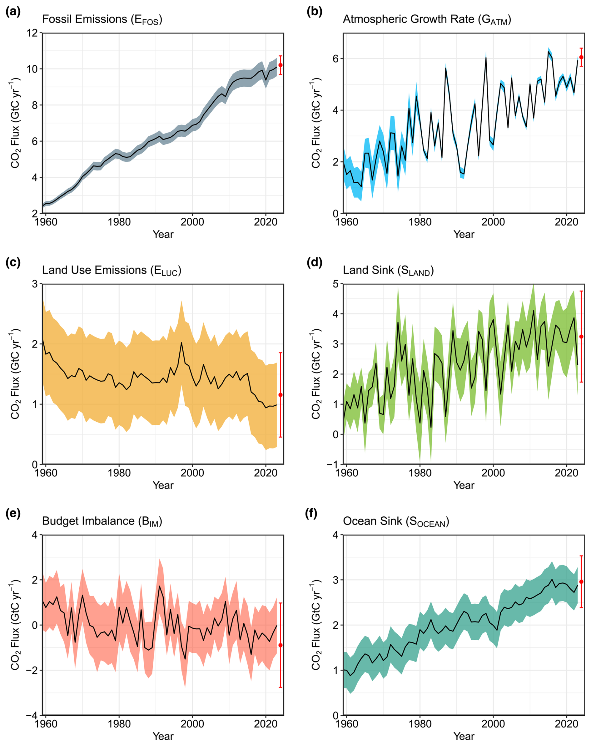
Figure 4 Components of the global carbon budget and their uncertainties as a function of time, presented individually for (a) fossil CO₂, including cement carbonation emissions (E_FOS); (b) the growth rate in atmospheric CO₂ concentration (G_ATM); (c) emissions from land-use change (E_LUC); (d) the land CO₂ sink (S_LAND); (e) the budget imbalance (B_IM) that is not accounted for by the other terms; and (f) the ocean CO₂ sink (S_OCEAN). Positive values of S_LAND and S_OCEAN represent a flux from the atmosphere to land or the ocean. All data are in GtC yr⁻¹ with the uncertainty bounds representing ±1 standard deviation in shaded colour. Data sources are as in Fig. 3. The red dots indicate our projections for the year 2024 and the red error bars the uncertainty in the 2024 projections (see Methods).

3.1.2 Recent period 1960–2023

Global fossil CO₂ emissions, E_FOS (including the cement carbonation sink), have increased every decade from an average of 3.0 ± 0.2 GtC yr⁻¹ for the decade of the 1960s to an average of 9.7 ± 0.5 GtC yr⁻¹ during 2014–2023 (Table 7, Figs. 2 and 5). The growth rate in these emissions decreased between the 1960s and the 1990s, from 4.3 % yr⁻¹ in the 1960s (1960–1969), 3.2 % yr⁻¹ in the 1970s (1970–1979), and 1.6 % yr⁻¹ in the 1980s (1980–1989) to 1.0 % yr⁻¹ in the 1990s (1990–1999). After this period, the growth rate began increasing again in the 2000s at an average growth rate of 2.8 % yr⁻¹, decreasing to 0.6 % yr⁻¹ for the last decade (2014–2023). China's emissions increased by +1.9 % yr⁻¹ on average over the last 10 years, dominating the global trend, and India's emissions increased by +3.6 % yr⁻¹, while emissions decreased in EU27 (the 27 countries of the EU) by 2.1 % yr⁻¹ and in the USA by 1.2 % yr⁻¹. Figure 6 illustrates the spatial distribution of fossil fuel emissions for the 2014–2023 period.

E_FOS reported here includes the uptake of CO₂ by cement via carbonation, which has increased with increasing stocks of cement products from an average of 20 MtC yr⁻¹ (0.02 GtC yr⁻¹) in the 1960s to an average of 200 MtC yr⁻¹ (0.2 GtC yr⁻¹) during 2014–2023 (Fig. 5).

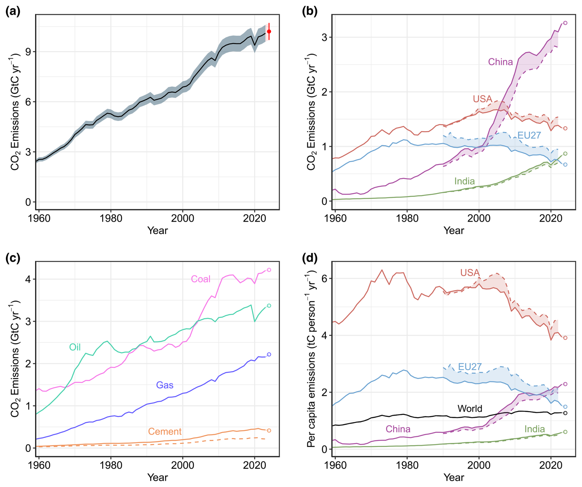
Figure 5 Fossil CO₂ emissions for (a) the globe, including an uncertainty of ±5 % (grey shading) and a projection through the year 2024 (red dot and uncertainty range); (b) territorial (solid lines) and consumption (dashed lines) emissions for the top three country emitters (USA, China, India) and for the European Union (EU27); (c) global emissions by fuel type, including coal, oil, gas, cement, and cement minus cement carbonation (dashed); and (d) per capita emissions for the world and for the large emitters as in panel (b). Territorial emissions are primarily from a draft update of Hefner and Marland (2023), except for national data for most Annex I countries for 1990–2022, which are reported to the UNFCCC as detailed in the text, as well as some improvements in individual countries, and are extrapolated forward to 2023 using data from the Energy Institute. Consumption-based emissions are updated from Peters et al. (2011). See Sects. 2.1 and S1 for details of the calculations and data sources.

3.1.3 Final year 2023

Global fossil CO₂ emissions were slightly higher, 1.4 %, in 2023 than in 2022, with an increase of 0.14 GtC to reach 10.1 ± 0.5 GtC (including the 0.21 GtC cement carbonation sink) in 2023 (Fig. 5), distributed among coal (41 %), oil (32 %), natural gas (21 %), cement (4 %), flaring (< 1 %), and others (< 1 %). Compared to 2022, the 2023 emissions from coal, oil, and gas increased by 1.4 %, 2.5 %, and 0.1 %, respectively, while emissions from cement decreased by 2 %. All annual growth rates presented are adjusted for the leap year, unless stated otherwise.

In 2023, the largest absolute contributions to global fossil CO₂ emissions were from China (31 %), the USA (13 %), India (8 %), and EU27 (7 %). These four regions account for 59 % of global fossil CO₂ emissions, while the rest of the world contributed 41 %, including international aviation and marine bunker fuels (3 % of the total). Growth rates for these countries/regions from 2022 to 2023 were 4.9 % (China), −3.3 % (USA), −8.4 % (EU27), and 8.2 % (India), with +0.7 % for the rest of the world, including international aviation and marine bunker fuels (+9.5 %). The per capita fossil CO₂ emissions in 2023 were 1.3 tC per person per year for the globe and were 3.9 (USA), 2.3 (China), 1.5 (EU27), and 0.6 (India) tC per person per year for the four highest emitters (Fig. 5).

3.1.4 Year 2024 projection

Globally, we estimate that global fossil CO₂ emissions (including cement carbonation, −0.21 GtC) will grow by 0.8 % in 2024 (−0.2 % to +1.7 %) to 10.2 GtC (37.4 GtCO₂), a historical record high.² Carbon Monitor projects a comparable 2024 increase of 0.8 % (0.5 % to 1.1 %). GCB estimates of changes in 2024 emissions per fuel type, relative to 2023, are projected to be 0.1 % (range −1.0 % to 1.2 %) for coal, +0.9 % (range 0.3 % to 1.6 %) for oil, +2.5 % (range 1.3 % to 3.8 %) for natural gas, and −3.5 % (range −5.3 % to −1.6 %) for cement.

For China, projected fossil emissions in 2024 are expected to increase slightly by 0.1 % (range −1.7 % to 1.9 %) compared with 2023 emissions, bringing 2023 emissions for China to around 3.3 GtC yr⁻¹ (11.9 GtCO₂ yr⁻¹). In contrast, the Carbon Monitor estimate projects a 2024 decrease of 0.8 % (range −1.3 % to −1.4 %). Our projected changes by fuel for China are +0.4 % for coal, −1.0 % for oil, +7.6 % for natural gas, and −9.4 % for cement.

For the USA, using the Energy Information Administration (EIA) emissions projection for 2024 combined with cement clinker data from USGS, we project a decrease of 0.9 % (range −2.1 % to 0.3 %) compared to 2023, bringing USA 2023 emissions to around 1.3 GtC yr⁻¹ (4.9 GtCO₂ yr⁻¹). Conversely, Carbon Monitor projects a 2024 increase of 1.3 % (1.0 % to 1.6 %). Our projected changes by fuel are −5.7 % for coal, −0.7 % for oil, +1.1 % for natural gas, and −7.1 % for cement.

For the European Union, our projection for 2024 is for a decrease of 2.8 % (range −5.2 % to −0.3 %) relative to 2023, with 2024 emissions around 0.7 GtC yr⁻¹ (2.4 GtCO₂ yr⁻¹). The Carbon Monitor projection for EU27 is slightly lower than that of the GCB, with a decrease of 4.5 % (−5.4 % to −3.6 %). Our projected changes by fuel are −11.3 % for coal, −0.6 % for oil, +0.4 % for natural gas, and −3.1 % for cement.

For India, our projection for 2024 is an increase of 3.7 % (range of 3.3 % to 4.0 %) over 2023, with 2024 emissions around 0.9 GtC yr⁻¹ (3.2 GtCO₂ yr⁻¹). The Carbon Monitor projection for India is an increase of 5.0 % (4.4 % to 5.5 %). Our projected changes by fuel are +3.3 % for coal, +3.3 % for oil, +11.8 % for natural gas, and +3.8 % for cement.

International aviation and shipping are projected to increase by 7.8 % in 2024, reaching 0.3 GtC yr⁻¹ (1.2 GtCO₂ yr⁻¹), with international aviation projected to be up 14 % over 2023, continuing to recover from pandemic lows, and international shipping projected to rise by 3 %. The Carbon Monitor projects international aviation and shipping to only increase by 2.6 % in 2024.

For the rest of the world, the expected change for 2024 is an increase of 1.2 % (range −0.7 % to 3.2 %), with 2024 emissions around 4.0 GtC yr⁻¹ (14.5 GtCO₂ yr⁻¹), which is similar to the Carbon Monitor projection of 1.5 % (range −1.2 % to 1.8 %). The fuel-specific projected 2024 growth rates for the rest of the world are +0.5 % for coal, +0.8 % for oil, +2.2 % for natural gas, and +2.0 % for cement.

For traceability, Table S6 provides a comparison of annual projections from the GCB since 2015 with the actual emissions assessed in the subsequent GCB annual report.

3.2 Emissions from land-use change

3.2.1 Historical period 1850–2023

Cumulative CO₂ emissions from land-use change (E_LUC) for 1850–2023 were 225 ± 65 GtC (Table 8; Figs. 3, 16). The cumulative emissions from E_LUC show a large spread among individual estimates of 150 GtC (H&C2023), 205 GtC (OSCAR), 250 GtC (LUCE), and 285 GtC (BLUE) for the four bookkeeping models and a similar wide estimate of 250 ± 85 GtC for the DGVMs (all cumulative numbers are rounded to the nearest 5 GtC). Vegetation biomass observations provide independent constraints on the E_LUC estimates (Li et al., 2017). Over the 1901–2012 period, the GCB bookkeeping models' cumulative E_LUC amounts to 165 [105, 210] GtC, which is similar to the observation-based estimate of 155 ± 50 GtC (Li et al., 2017).

3.2.2 Recent period 1960–2023

In contrast to growing fossil emissions, CO₂ emissions from land-use, land-use change, and forestry remained relatively constant (around 1.5 GtC yr⁻¹) over the 1960–1999 period. Since then, they have shown a statistically significant decrease of about 0.2 GtC per decade, reaching 1.1±0.7 GtC yr⁻¹ for the 2014–2023 period (Table 7), but with significant spread from 0.8 to 1.3 GtC yr⁻¹, across the four bookkeeping models (Table 5, Fig. 7). Differently from the bookkeeping average, the DGVM average grows slightly larger over the 1980–2010 period and shows no sign of decreasing emissions in the recent decades, apart from in the most recent decade (Table 5, Fig. 7). This is, however, expected as DGVM-based estimates include the loss of additional sink capacity, which grows with time, while the bookkeeping estimates do not (Supplement, Sect. S6.4).

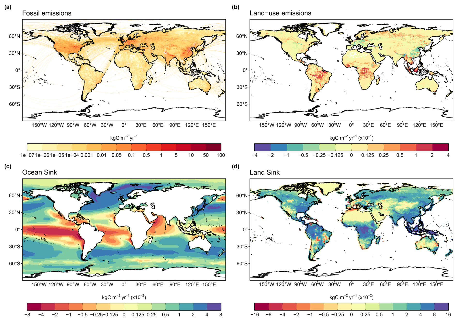
Figure 6 The 2014–2023 decadal mean components of the global carbon budget, presented for (a) fossil CO₂ emissions (E_FOS), (b) land-use change emissions (E_LUC), (c) the ocean CO₂ sink (S_OCEAN), and (d) the land CO₂ sink (S_LAND). Positive values for E_FOS and E_LUC represent a flux to the atmosphere, whereas positive values of S_OCEAN and S_LAND represent a flux from the atmosphere to the ocean or the land (carbon sink). In all panels, yellow and red colours represent a source (flux from the land and ocean to the atmosphere) and green and blue colours represent a sink (flux from the atmosphere into the land and ocean). All units are in kgC m⁻² yr⁻¹. Note the different scales in each panel. E_FOS data shown are from GCP-GridFEDv2024.0 and do not include cement carbonation. The E_LUC map shows the average E_LUC from the four bookkeeping models and emissions from peat drainage and peat fires. BLUE and LUCE provide spatially explicit estimates at 0.25° resolution. Gridded E_LUC estimates for H&C2023 and OSCAR are derived by spatially distributing their national data based on the spatial patterns of BLUE gross fluxes in each country (see Schwingshackl et al., 2022, for more details about the methodology). S_OCEAN data shown are the average of GOBM and fCO₂-product means, using GOBM simulation A, no adjustment for bias, and drift applied to the gridded fields (see Sect. 2.5). S_LAND data shown are the average of the DGVMs (see Sect. 2.6).

Table 5 Comparison of results from the bookkeeping method and budget residuals with results from the DGVMs, as well as additional estimates from atmospheric oxygen, atmospheric inversions and Earth system models (ESMs) for different periods, the last decade, and the last year available. All values are in GtC yr⁻¹. See Fig. 7 for explanation of the bookkeeping component fluxes. The DGVM uncertainties represent ±1σ of the decadal or annual (for 2023) estimates from the individual DGVMs: for the inverse systems, the mean and range of available results are given. All values are rounded to the nearest 0.1 GtC, and therefore columns do not necessarily add to zero.

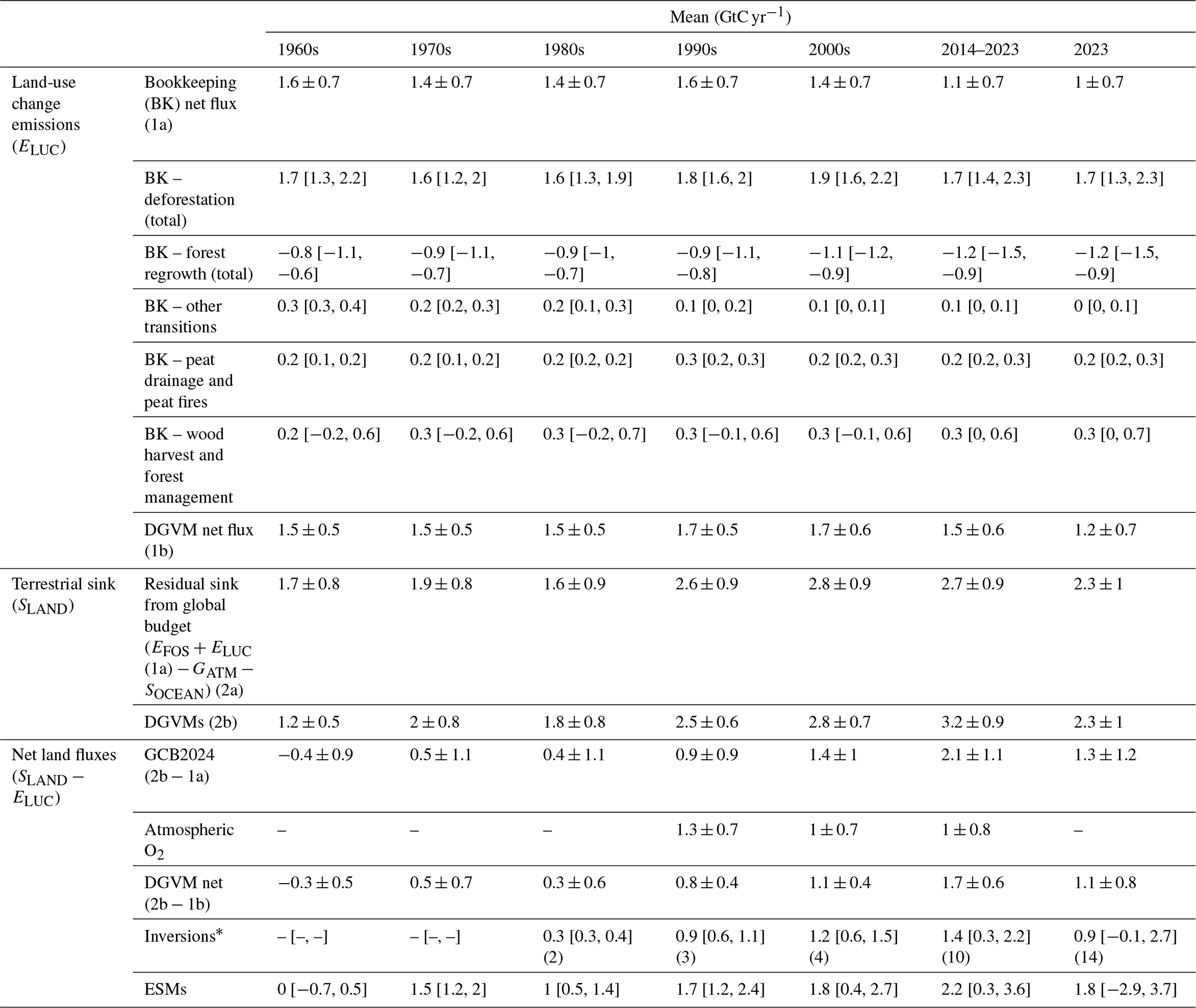
^∗ Estimates are adjusted for the pre-industrial influence of river fluxes and for the cement carbonation sink and are adjusted to a common E_FOS (Sect. 2.7). The ranges given include varying numbers (in parentheses) of inversions in each decade (Table S4).

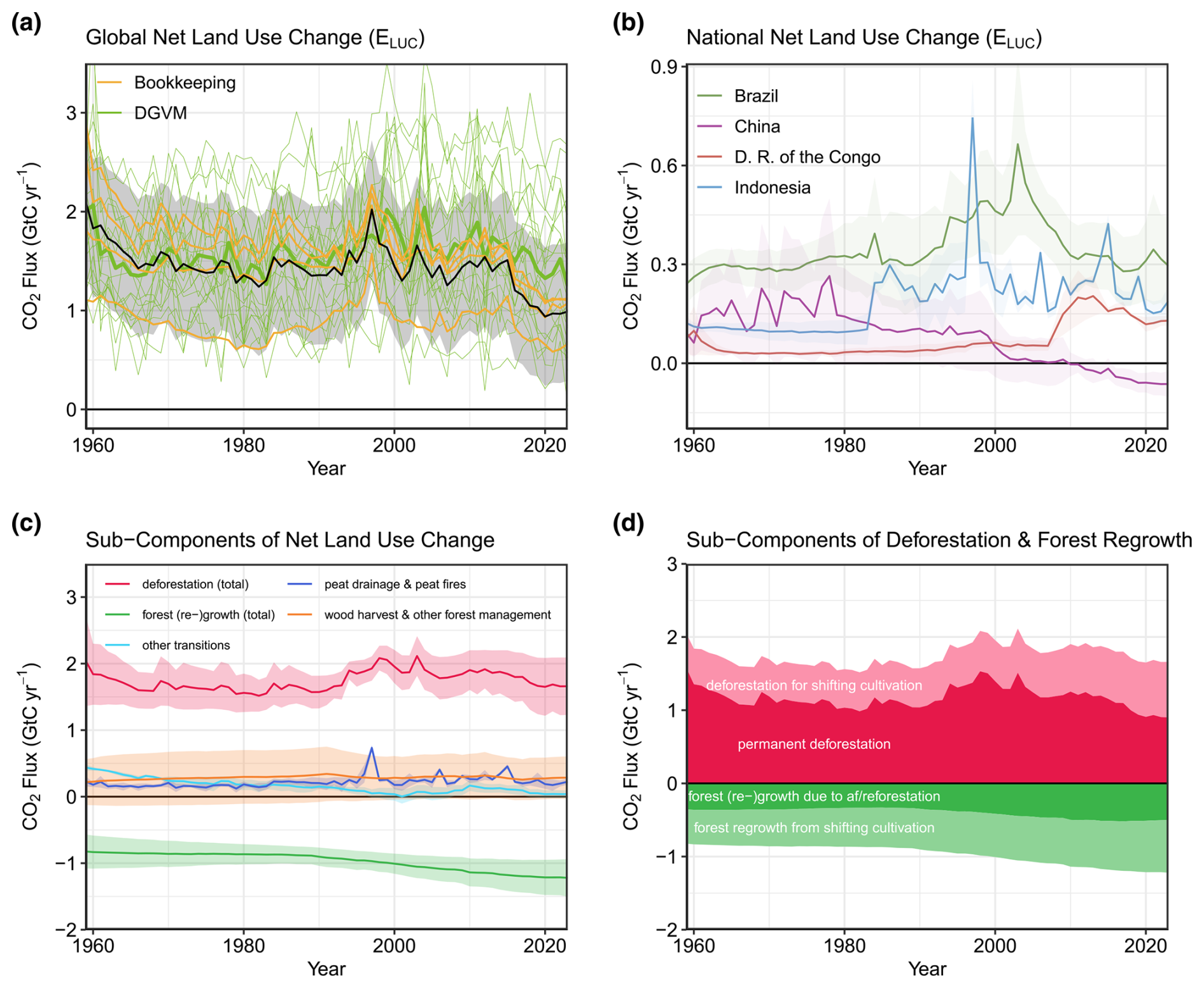
Figure 7 Net CO₂ exchanges between the atmosphere and the terrestrial biosphere related to land-use change. (a) Net CO₂ emissions from land-use change (E_LUC) with estimates from the four bookkeeping models (yellow lines) and the budget estimate (black with ±1σ uncertainty), which is the average of the four bookkeeping models. Estimates from individual DGVMs (narrow green lines) and the DGVM ensemble mean (thick green line) are also shown. (b) Net CO₂ emissions from land-use change from the four countries/regions with the largest cumulative emissions since 1959. Values shown are the average of the four bookkeeping models, with shaded regions as ±1σ uncertainty. (c) Subcomponents of E_LUC: (i) emissions from deforestation (including permanent deforestation and deforestation in shifting cultivation cycles), (ii) emissions from peat drainage and peat fires, (iii) removals from forest (re)growth (including forest (re)growth due to afforestation and reforestation and forest regrowth in shifting cultivation cycles), (iv) fluxes from wood harvest and other forest management (comprising slash and product decay following wood harvest, regrowth after wood harvest, and fire suppression), and (v) emissions and removals related to other land-use transitions. The sum of the five components is E_LUC shown in panel (a). (d) Subcomponents of “deforestation (total)” and of “forest (re)growth (total)”: (i) deforestation in shifting cultivation cycles, (ii) permanent deforestation, (iii) forest (re)growth due to afforestation and/or reforestation, and (iv) forest regrowth in shifting cultivation cycles.

We separate net E_LUC into five component fluxes to gain further insight into the drivers of net emissions: deforestation, forest (re)growth, wood harvest and other forest management, peat drainage and peat fires, and all other transitions (Fig. 7c; Supplement, Sect. S2.1). We further decompose the deforestation and the forest (re)growth term into contributions from shifting cultivation vs. permanent forest cover changes (Fig. 7d). Averaged over the 2014–2023 period and over the four bookkeeping estimates, fluxes from deforestation amount to 1.7 [1.4, 2.3] GtC yr⁻¹ (Table 5), of which 1.0 [0.8, 1.1] GtC yr⁻¹ is from permanent deforestation. Fluxes from forest (re)growth amount to −1.2 [−1.5, −0.9] GtC yr⁻¹ (Table 5), of which −0.5 [−0.7, −0.3] GtC yr⁻¹ is from re-/afforestation and the remainder is from forest regrowth in shifting cultivation cycles. Emissions from wood harvest and other forest management (0.3 [0.0, 0.6] GtC yr⁻¹) and peat drainage and peat fires (0.2 [0.2, 0.3] GtC yr⁻¹) and the net flux from other transitions (0.1 [0.0, 0.1] GtC yr⁻¹) are substantially less important globally (Table 5). However, the small net flux from wood harvest and other forest management contains substantial gross fluxes that largely compensate for each other (see Fig. S8): 1.4 [0.9, 2.0] GtC yr⁻¹ of emissions result from the decomposition of slash and the decay of wood products and −1.1 [−1.4, −0.8] GtC yr⁻¹ of removals result from regrowth after wood harvesting.

The split into component fluxes clarifies the potential for emissions reduction and carbon dioxide removal: the emissions from permanent deforestation – the largest of our component fluxes – could be halted (largely) without compromising carbon uptake by forests, contributing substantially to emissions reduction. By contrast, reducing wood harvesting would have limited potential to reduce emissions as it would be associated with less forest regrowth; removals and emissions cannot be decoupled here on long timescales. A similar conclusion applies to removals and emissions from shifting cultivation, which we have therefore separated out. Carbon dioxide removal (CDR) in forests could instead be increased by permanently increasing the forest cover through re-/afforestation. Our estimate of about −0.5 GtC yr⁻¹ removed on average each year during 2014–2023 by re-/afforestation is similar to independent estimates that were derived from NGHGIs for CDR in managed forests (through re-/afforestation and forest management) for 2013–2022 (−0.5 GtC yr⁻¹; Pongratz et al., 2024). Re-/afforestation constitutes the vast majority of all current CDR (Pongratz et al., 2024). Though transfers between non-atmospheric reservoirs cannot be compared directly to annual fluxes from the atmosphere and are thus not included in our estimate of E_LUC, CDR through these reservoirs such as in durable HWPs, biochar, or BECCS comprise much smaller amounts of carbon. A total of 218 MtC yr⁻¹ has been estimated to be transferred to HWPs, averaged over 2013–2022 (Pongratz et al., 2024). The net flux of HWPs, considering the re-release of CO₂ through their decay, amounts to 91 MtC yr⁻¹ over that period (Pongratz et al., 2024). Note that some double counting between the CDR through HWPs and the CDR through re-/afforestation exists if the HWPs are derived from newly forested areas. BECCS projects have been estimated to have stored 0.1 MtC yr⁻¹ in geological projects worldwide in 2023 and biochar projects 0.2 MtC yr⁻¹ (Pongratz et al., 2024). “Blue carbon”, i.e. coastal wetland management such as restoration of mangrove forests, salt marshes, and seagrass meadows, though at the interface of land and ocean carbon fluxes, is counted towards the land-use sector as well. Currently, bookkeeping models do not include blue carbon; however, current CDR deployment in coastal wetlands is small globally, less than 0.003 MtC yr⁻¹ (Powis et al., 2023).

The statistically significant decrease in E_LUC since the late 1990s, including the larger drop within the most recent decade, is due to the combination of decreasing emissions from deforestation (in particular permanent deforestation) and increasing removals from forest regrowth (with those from re-/afforestation stagnating globally in the last decade). Emissions in 2014–2023 are 28 % lower than in the late 1990s (1995–2004) and 20 % lower than in 2004–2013. The steep drop in E_LUC after 2015 is due to the combined effect from a peak in peat fire emissions in 2015 and a long-term decline in deforestation emissions in many countries over the 2010–2020 period, with the largest declines in the Democratic Republic of the Congo, Brazil, China, and Indonesia. Since the processes behind gross removals, foremost forest regrowth and soil recovery, are all slow, while gross emissions include a large instantaneous component, short-term changes in land-use dynamics, such as a temporary decrease in deforestation, influences gross emissions dynamics more than gross removal dynamics, which rather are a response to longer-term dynamics. Component fluxes often differ more across the four bookkeeping estimates than the net flux, which is expected due to different process representation; in particular, the treatment of shifting cultivation, which increases both gross emissions and removals, differs across models, but net and gross wood harvest fluxes also show high uncertainty. By contrast, models agree relatively well for emissions from permanent deforestation.

Overall, the highest land-use emissions occur in the tropical regions of all three continents. The top three emitters (both cumulatively 1959–2023 and on average over 2014–2023) are Brazil (in particular the Amazon arc of deforestation), Indonesia, and the Democratic Republic of the Congo, with these three countries contributing 0.7 GtC yr⁻¹ or 60 % of the global net land-use emissions (average over 2014–2023) (Figs. 6b, 7b). This is related to massive expansion of cropland, particularly in the last few decades in Latin America, Southeast Asia, and sub-Saharan Africa (Hong et al., 2021), with a substantial part for export of agricultural products (Pendrill et al., 2019). Emissions intensity is high in many tropical countries, particularly in Southeast Asia, due to high rates of land conversion in regions of carbon-dense and often still pristine, undegraded natural forests (Hong et al., 2021). Emissions are further increased by peat fires in equatorial Asia (GFED4.1s; van der Werf et al., 2017). Our estimates of high E_LUC in China have been revised down since the 1980s as compared to GCB2023, which is related to the update of the land-use forcing, now based on the cropland dataset by Yu et al. (2022) (see the Supplement, Sect. S2.2); this suggests lower cropland expansion and thus less deforestation than the previous datasets assumed. Uptake due to land-use change occurs in several regions of the world (Fig. 6b) particularly because of re-/afforestation. The highest CDR in the last decade is seen in China, where our estimates show an even larger uptake since 2010 compared to GCB2023, related to the updated land-use forcing in EU27, which is partly related to expanding forest area as a consequence of the forest transition in the 19th and 20th centuries and subsequent regrowth of forest (Mather, 2001; McGrath et al., 2015), and in the USA. Substantial uptake through re-/afforestation also exists in other regions such as Brazil, Myanmar, or Russia, where, however, emissions from deforestation and other land-use changes dominate the net flux.

While the mentioned patterns are robust and supported by independent literature, we acknowledge that model spread is substantially larger on regional than on global levels, as has been shown for bookkeeping models (Bastos et al., 2021) as well as DGVMs (Obermeier et al., 2021). Assessments for individual regions are being performed as part of REgional Carbon Cycle Assessment and Processes (RECCAP-2; Ciais et al., 2022; Poulter et al., 2022) or already exist for selected regions (e.g. for Europe by Petrescu et al., 2020; for Brazil by Rosan et al. (2021); for eight selected countries/regions in comparison to inventory data by Schwingshackl et al., 2022). The revisions since GCB2023 reflect such uncertainties: the integration of a fourth bookkeeping model alters our estimates, though only to a limited extent given that the new model LUCE lies in between the other three models for the global E_LUC estimates. Larger changes are obvious at a regional level due to the revisions of the land-use forcing, with a general update to more recent FAO input for agricultural areas and wood harvest, new MapBiomas input for Brazil and Indonesia, and the updated cropland dataset in China.

The NGHGI data under the LULUCF sector and the LULUCF estimates from FAOSTAT differ from the global models' definition of E_LUC (see Sect. 2.2.1). In the NGHGI reporting, the natural fluxes (S_LAND) are counted towards E_LUC when they occur on managed land (Grassi et al., 2018). To compare our results to the NGHGI approach, we perform a translation of our E_LUC estimates by adding S_LAND in managed forest from the DGVM simulations (following the methodology described in Grassi et al., 2023) to the bookkeeping E_LUC estimate (see the Supplement, Sect. S2.3). For the 2014–2023 period, we estimate that 1.8 GtC yr⁻¹ of S_LAND occurred in managed forests. Adding this sink to E_LUC changes E_LUC from being a source of 1.1 GtC yr⁻¹ to a sink of 0.7 GtC yr⁻¹, which is very similar to the NGHGI estimate that yields a sink of 0.8 GtC yr⁻¹ (Fig. 8, Table S10). We further apply a mask of managed land to the net atmosphere-to-land flux estimate from atmospheric inversions to obtain inverse estimates that are comparable to the NGHGI estimates and to the translated E_LUC estimates from bookkeeping models (see the Supplement, Sect. S2.3). The inversion-based net flux in managed land indicates a sink of 0.7 GtC yr⁻¹ for 2014–2023, which agrees very well with the NGHGIs and the translated E_LUC estimates (Fig. 8, Table S10). Additionally, the interannual variability in the inversion estimates and that in the translated E_LUC estimates show remarkable agreement (Pearson correlation of 0.81 in 2000–2023), which supports the suggested translation approach.

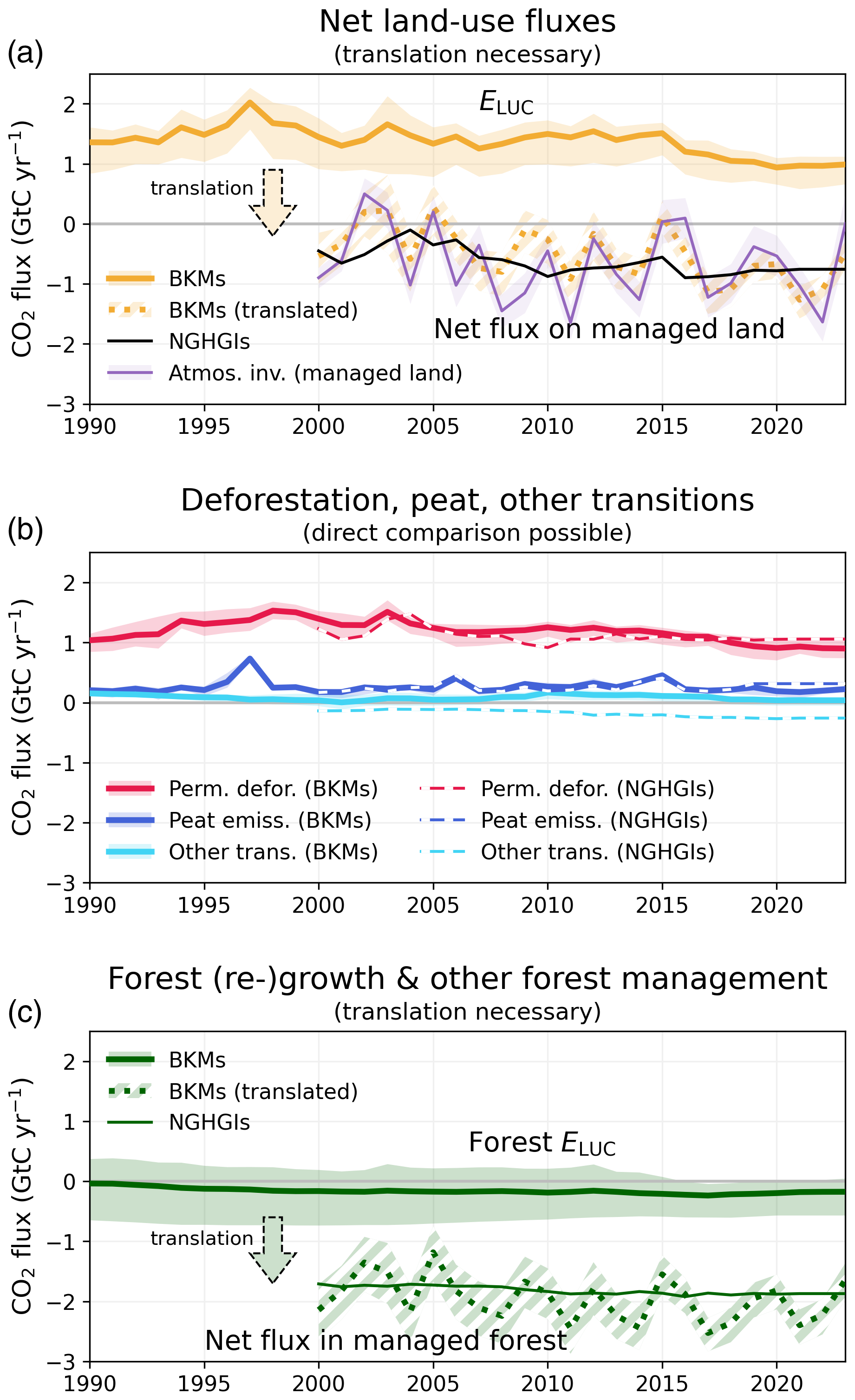
Figure 8 Comparison of land-use flux estimates from bookkeeping models (BKMs; following the GCB definition of E_LUC), national GHG inventories (NGHGIs; following IPCC guidelines and thus including all carbon fluxes on managed land), and atmospheric inversion systems (considering fluxes on managed land only). To compare BKM results with NGHGIs, a translation is necessary for some subcomponents. (a) Net land-use fluxes, for which a translation of BKMs is necessary; (b) permanent deforestation, peat drainage and peat fire, and other transition subcomponents, which can be directly compared; and (c) the forest (re)growth and other forest management subcomponent, for which a translation is necessary. The lines represent the mean of 4 BKMs and 14 atmospheric inversion estimates; shaded areas denote the full range across BKM estimates and the standard deviation for atmospheric inversions. The subcomponent forest (re)growth and other forest management includes removals from forest (re)growth (permanent), emissions and removals from wood harvest and other forest management, and emissions and removals in shifting cultivation cycles. The translation of BKM estimates to NGHGI estimates in (a) and (c) is done by adding the natural land sink in managed forests to the BKM estimates (see also Table S10). The GCB definition of E_LUC and the NGHGI definition of land-use fluxes are equally valid, each in its own context. For illustrative purposes we only show the translation of BKM estimates to the NGHGI definition.

The translation approach has been shown to also be generally applicable at the country level (Grassi et al., 2023; Schwingshackl et al., 2022). Country-level analysis suggests, for example, that the bookkeeping method estimates higher deforestation emissions than the national report in Indonesia but less CO₂ removal by afforestation than the national report in China. The fraction of the natural CO₂ sinks that the NGHGI estimates include differs substantially across countries, related to varying proportions of managed vs. total forest areas (Schwingshackl et al., 2022). By comparing E_LUC and NGHGI on the basis of the component fluxes used above, we find that our estimates very closely reproduce the NGHGI estimates for emissions from permanent deforestation, peat emissions, and other transitions (Fig. 8), although a difference in sign for the latter (small source in bookkeeping estimates, small sink in NGHGI) creates a notable difference between NGHGI and bookkeeping estimates. Fluxes due to forest (re)growth and other forest management, that is, (re)growth from re-/afforestation and the net flux from wood harvesting and other forest management and emissions and removals in shifting cultivation cycles, constitute a large sink in the NGHGI (−1.9 GtC yr⁻¹ averaged over 2014–2023), since they also include S_LAND in managed forests. Summing up the bookkeeping estimates of (re)growth from re-/afforestation, the net flux from wood harvesting and other forest management, and the emissions and removals in shifting cultivation cycles and adding S_LAND in managed forests yields a flux of −2.0 GtC yr⁻¹ (averaged over 2014–2023), which compares well with the NGHGI estimate. Though estimates between NGHGI, FAOSTAT, and the translated budget estimates still differ in value and need further analysis, the approach suggested by Grassi et al. (2023), which we adopt here, provides a feasible way to relate the global models' and NGHGI approaches to each other and thus link the anthropogenic carbon budget estimates of land CO₂ fluxes directly to the Global Stocktake as part of the UNFCCC Paris Agreement.

3.2.3 Final year 2023

The global CO₂ emissions from land-use change are estimated as 1.0±0.7 GtC in 2023, which is similar to the 2022 estimate. However, confidence in the annual change remains low. Despite El Niño conditions, which in general lead to more fires in deforestation areas, peat fire emissions in Indonesia remained below average (GFED4.1s; updated from van der Werf et al., 2017). In South America, emissions from tropical deforestation and degradation fires have been about average, as effects of the El Niño in the Amazon, such as droughts, are not expected before 2024.

3.2.4 Year 2024 projection

In Southeast Asia, peat fire emissions have further dropped (from 27 TgC in 2023 to 2 TgC in 2024 through 31 December 2024; GFED4.1s – van der Werf et al., 2017), as have tropical deforestation and degradation fires (from 33 to 8 TgC) as the El Niño conditions ceased. By contrast, emissions from tropical deforestation and degradation fires in South America have risen from 121 TgC in 2023 to 334 TgC in 2024 up until 31 December, as the impacts of the El Niño unfolded, in particular drought conditions since 2023. The 2024 South American fire emissions are among the highest values in the record, which started in 1997. Part of the increase is due to elevated fire activity in the wetlands of the Pantanal. Disentangling the degree to which interannual variability in rainfall patterns and stronger environmental protection measures in both Indonesia after their 2015 high-fire-activity season and Brazil after the change in government play a role in fire trends is an important research topic. Cumulative 2024 fire emissions estimates through 31 December 2024 are 439 TgC for global deforestation and degradation fires and 2 TgC for peatland fires in Southeast Asia.

Based on these estimates, we expect E_LUC emissions of around 1.2 GtC (4.2 GtCO₂) in 2024, 0.17 GtC above the 2023 level. Note that although our extrapolation includes tropical deforestation and degradation fires, the degradation attributable to selective logging, edge effects, or fragmentation is not captured. Further, deforestation and fires in deforestation zones may become more disconnected, partly due to changes in legislation in some regions. For example, van Wees et al. (2021) found that the contribution from fires to forest loss decreased in the Amazon and in Indonesia over the period of 2003–2018.

Table 6 Comparison of results for the ocean sink from the fCO₂ products, from global ocean biogeochemistry models (GOBMs); the best estimate for GCB2024 as calculated from fCO₂ products and GOBMs that is used in the budget (Table 7); and additional estimates from atmospheric oxygen, atmospheric inversions, and Earth system models (ESMs) for different periods, the last decade, and the last year available. All values are in GtC yr⁻¹. Uncertainties represent ±1σ of the estimates from the GOBMs (N>10), and the range of ensemble members is given for ensembles with N<10 (fCO₂ products, inversions, ESMs). The uncertainty in the GCB2024 budget estimate is based on expert judgement (Sects. 2 and S1 to S4), and for oxygen it is the standard deviation of a Monte Carlo ensemble (Sect. 2.8).

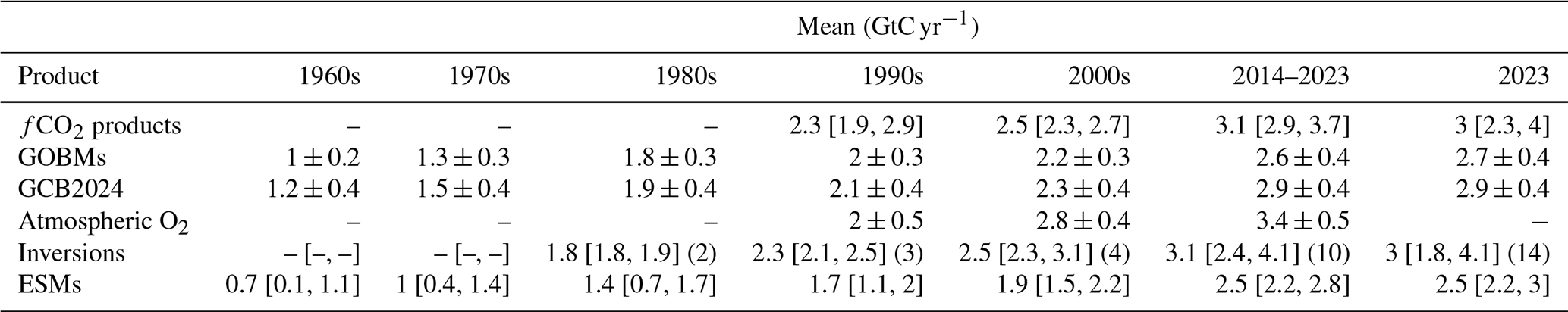
3.3 CDR not based on vegetation

Besides the CDR through land use (Sect. 3.2), the atmosphere-to-geosphere flux of carbon resulting from carbon dioxide removal (CDR) activity in 2023 is estimated at 0.011 MtC yr⁻¹. This results primarily from 0.009 MtC yr⁻¹ of enhanced-weathering projects and 0.001 MtC yr⁻¹ of DACCS. While it represents a growth of 200 % in the anthropogenic sink from the 0.0036 MtC yr⁻¹ estimate in 2022, it remains about a million times smaller than current fossil CO₂ emissions. Note that the lower estimate for DACCS is due to more accurate (lower) annual estimates now being available rather than to lower activity. Enhanced rock weathering has gone up relative to last year, as a result of both better coverage of projects and an actual increase in activity.

3.4 Total anthropogenic emissions

Cumulative anthropogenic CO₂ emissions (fossil and land use) for 1850–2023 totalled 710 ± 70 GtC (2605 ± 260 GtCO₂), of which 70 % (500 GtC) occurred since 1960 and 34 % (240 GtC) since 2000 (Tables 7 and 8). Total anthropogenic emissions more than doubled over the last 60 years, from 4.6 ± 0.7 GtC yr⁻¹ for the decade of the 1960s to an average of 10.8 ± 0.9 GtC yr⁻¹ during 2014–2023 and reaching 11.1 ± 0.9 GtC (40.6 ± 3.2 GtCO₂) in 2023. However, total anthropogenic CO₂ emissions have been stable over the last decade (zero growth rate over the 2014–2023 period), much slower than the 2.0 % growth rate over the previous decade (2004–2013).

During the historical period 1850–2023, 31 % of historical emissions were from land-use change and 69 % from fossil emissions. However, fossil emissions have grown significantly since 1960, while land-use changes have not, and consequently the contributions of land-use change to total anthropogenic emissions were smaller during recent periods, 18 % during the period 1960–2023 and down to 10 % over the last decade (2014–2023).

For 2024, we project global total anthropogenic CO₂ emissions from fossil and land-use changes to be around 11.4 GtC (41.6 GtCO₂), 2 % above the 2023 level. All values here include the cement carbonation sink (currently about 0.2 GtC yr⁻¹).

3.5 Atmospheric CO₂

3.5.1 Historical period 1850–2023

Atmospheric CO₂ concentration was approximately 278 parts per million (ppm) in 1750, reaching 300 ppm in the late 1900s, 350 ppm in the late 1980s, and 419.31 ± 0.1 ppm in 2023 (Lan et al., 2024; Fig. 1). The mass of carbon in the atmosphere increased by 51 % from 590 GtC in 1750 to 890 GtC in 2023. Current CO₂ concentrations in the atmosphere are unprecedented for the last 2 million years, and the current rate of atmospheric CO₂ increase is at least 10 times faster than at any other time during the last 800 000 years (Canadell et al., 2021).

3.5.2 Recent period 1960–2023

The growth rate in the atmospheric CO₂ level increased from 1.7 ± 0.07 GtC yr⁻¹ in the 1960s to 5.2 ± 0.02 GtC yr⁻¹ during 2014–2023, with important decadal variations (Table 7, Figs. 3 and 4). During the last decade (2014–2023), the growth rate in atmospheric CO₂ concentration continued to increase, albeit with large interannual variability (Fig. 4).

Table 7 Decadal mean in the five components of the anthropogenic CO₂ budget for different periods and the last year available. All values are in GtC yr⁻¹, and uncertainties are reported as ±1σ. Fossil CO₂ emissions include cement carbonation. The table also shows the budget imbalance (B_IM), which provides a measure of the discrepancies among the nearly independent estimates. A positive imbalance means the emissions are overestimated and/or the sinks are too small. All values are rounded to the nearest 0.1 GtC, and therefore columns do not necessarily add to zero.

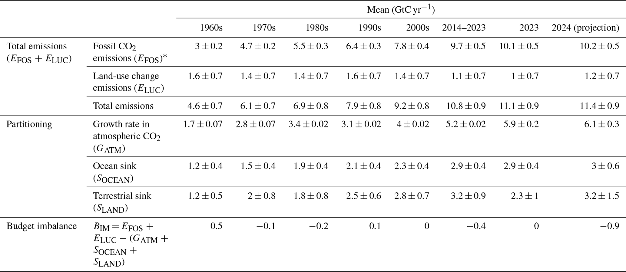
^∗ Fossil emissions excluding the cement carbonation sink amount to 3 ± 0.2, 4.7 ± 0.2, 5.5 ± 0.3, 6.4 ± 0.3, 7.9 ± 0.4, and 9.9 ± 0.5 GtC yr⁻¹ for the decades of the 1960s to 2010s, respectively, and to 10.3 ± 0.5 GtC yr⁻¹ for 2023 and 10.4 ± 0.5 GtC yr⁻¹ for 2024.

The airborne fraction (AF) is defined as the ratio of the atmospheric CO₂ growth rate to total anthropogenic emissions:

$$\begin{array}{}\text{(2)}& \mathrm{AF}=G_{\mathrm{ATM}}/(E_{\mathrm{FOS}}+E_{\mathrm{LUC}}).\end{array}$$

It provides a diagnostic of the relative strength of the land and ocean carbon sinks in removing part of the anthropogenic CO₂ perturbation. The evolution of AF over the last 60 years shows no significant trend, remaining at around 44 %, albeit showing a large interannual and decadal variability driven by the year-to-year variability in G_ATM (Fig. 10). The observed stability of the airborne fraction over the 1960–2023 period indicates that the ocean and land CO₂ sinks have been increasing in pace with the total anthropogenic emissions over that period, removing on average about 56 % of the emissions (see Sect. 3.6.2 and 3.7.2).

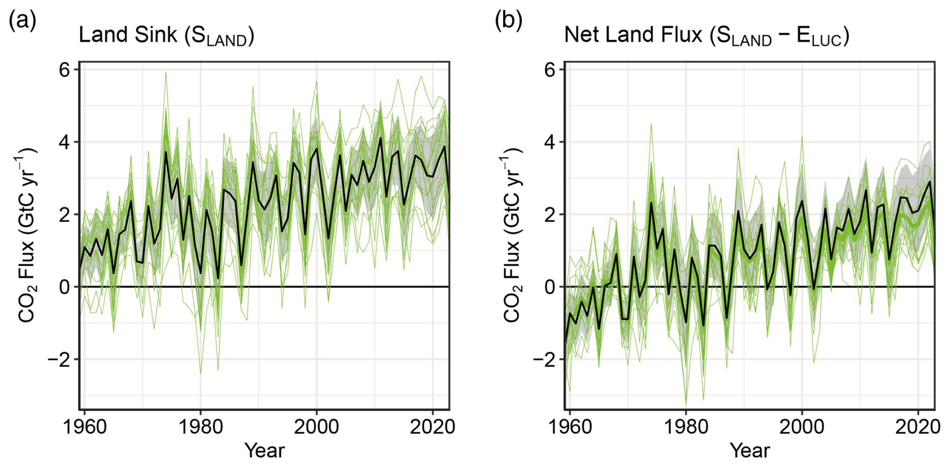
Figure 9 (a) The land CO₂ sink (S_LAND) estimated by individual DGVMs (green) as well as the budget estimate (black with ±1σ uncertainty), which is the average of all DGVMs. (b) Net atmosphere–land CO₂ fluxes (S_LAND – E_LUC). The budget estimate of the net land flux (black with ±1σ uncertainty) combines the DGVM estimate of S_LAND from panel (a) with the bookkeeping estimate of E_LUC from Fig. 7a. Uncertainties are similarly propagated in quadrature. DGVMs also provide estimates of E_LUC (see Fig. 7a), which can be combined with their own estimates of the land sink. Hence panel (b) also includes an estimate for the net land flux for individual DGVMs (thin green lines) and their multi-model mean (thick green line).

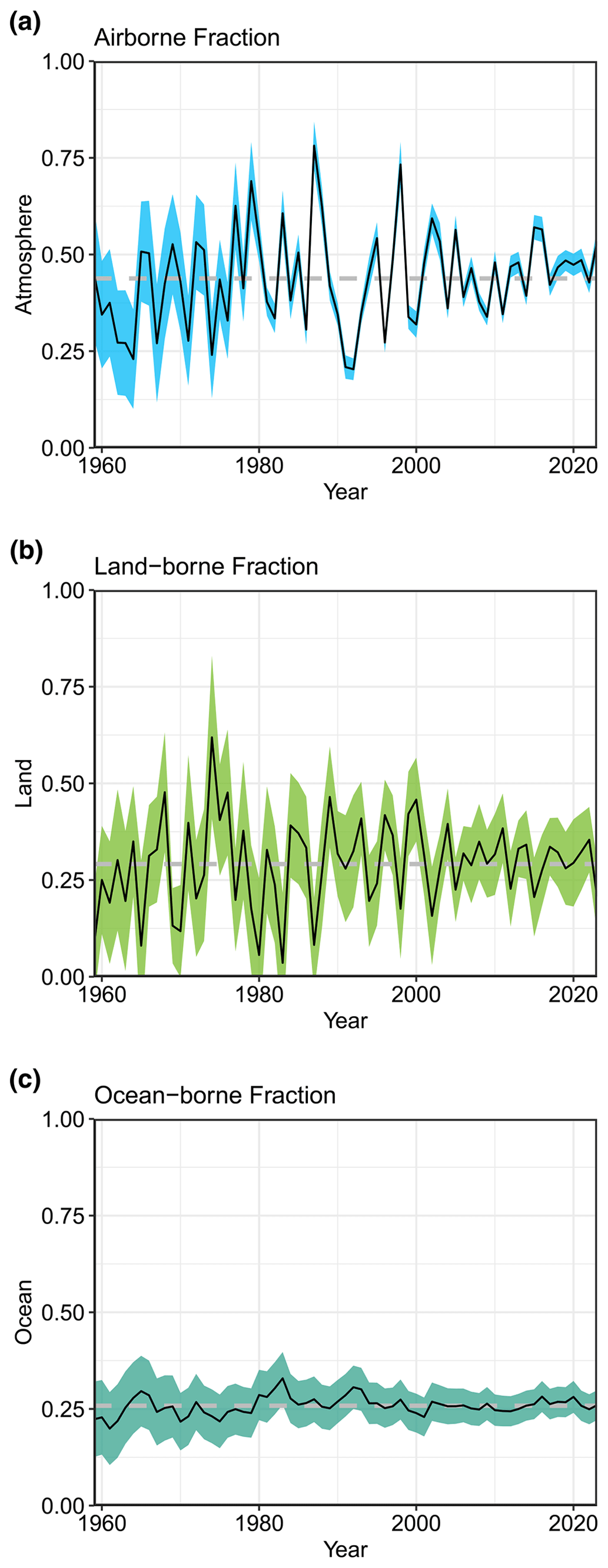
Figure 10 The partitioning of total anthropogenic CO₂ emissions (E_FOS+E_LUC) across the (a) atmosphere (airborne fraction), (b) land (land-borne fraction), and (c) ocean (ocean-borne fraction). Black lines represent the central estimate, and the coloured shading represents the uncertainty. The dashed grey lines represent the long-term average of the airborne (44 %), land-borne (30 %), and ocean-borne (25 %) fractions during 1960–2023 (with a B_IM of 1 %).

3.5.3 Final year 2023

The growth rate in atmospheric CO₂ concentration was 5.9 ± 0.2 GtC (2.79 ± 0.08 ppm) in 2023 (Fig. 4; Lan et al., 2024), well above the 2022 growth rate (4.6 ± 0.2 GtC) or the 2014–2023 average (5.2 ± 0.02 GtC), as to be expected during an El Niño year. The 2023 atmospheric CO₂ growth rate was the fourth largest over the 1959–2023 atmospheric observational record, closely following 2015, 2016, and 1998, all strong El Niño years.

3.5.4 Year 2024 projection

The 2024 growth in atmospheric CO₂ concentration (G_ATM) is projected to be about 6.1 GtC (2.87 ppm), still high, which is common for the year after a strong El Niño year. This is the average of the GCB regression method (6.1 GtC, 2.85 ppm) and the ESM multi-model mean (6.1 GtC, 2.88 ppm). The 2024 atmospheric CO₂ concentration, averaged over the year, is expected to reach the level of 422.45 ppm, 52 % above the pre-industrial level.

3.6 Ocean sink

3.6.1 Historical period 1850–2023

Cumulated since 1850, the ocean sink adds up to 185 ± 35 GtC, with more than two-thirds of this amount (130 ± 25 GtC) being taken up by the global ocean since 1960. Over the historical period, the ocean sink increased in pace with the anthropogenic emissions exponential increase (Fig. 3). Since 1850, the ocean has removed 26 % of total anthropogenic emissions.

Table 8 Cumulative CO₂ for different time periods in gigatonnes of carbon (GtC). Fossil CO₂ emissions include cement carbonation. The budget imbalance (B_IM) provides a measure of the discrepancies among the nearly independent estimates. All values are rounded to the nearest 5 GtC, and therefore columns do not necessarily add to zero. Uncertainties are reported as follows: E_FOS is 5 % of cumulative emissions, E_LUC prior to 1959 is the 1σ spread from the DGVMs, E_LUC post-1959 is 0.7 × the number of years (where 0.7 GtC yr⁻¹ is the uncertainty in the annual E_LUC flux estimate), G_ATM uncertainty is held constant at 5 GtC for all time periods, S_OCEAN uncertainty is 20 % of the cumulative sink (20 % relates to the annual uncertainty of 0.4 GtC yr⁻¹, which is ∼ 20 % of the current ocean sink), and S_LAND is the 1σ spread from the DGVM estimates.

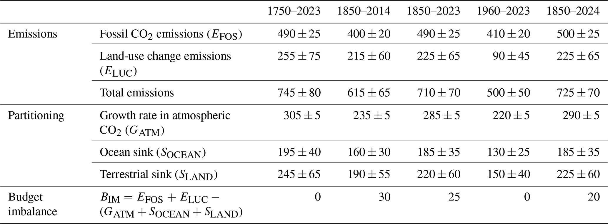
3.6.2 Recent period 1960–2023

The ocean CO₂ sink increased from 1.2 ± 0.4 GtC yr⁻¹ in the 1960s to 2.9 ± 0.4 GtC yr⁻¹ during 2014–2023 (Table 7), with interannual variations on the order of a few tenths of gigatonnes of carbon per year (Figs. 4, 11). The ocean-borne fraction ($S_{\mathrm{OCEAN}}/(E_{\mathrm{FOS}}+E_{\mathrm{LUC}}$)) has been remarkably constant at around 25 % on average (Fig. 10c), with variations around this mean illustrating the decadal variability in the ocean carbon sink. So far, there has been no indication of a decrease in the ocean-borne fraction from 1960 to 2022. The increase in the ocean sink is primarily driven by the increased atmospheric CO₂ concentration, with the strongest CO₂-induced signal in the North Atlantic and the Southern Ocean (Fig. 12a). The effect of climate change is much weaker, reducing the ocean sink globally by 0.17±0.05 GtC yr⁻¹ (−5.9 % of S_OCEAN) during 2014–2023 (all models simulate a weakening of the ocean sink by climate change, range −3.4 % to −10.7 %), and does not show clear spatial patterns across the GOBM ensemble (Fig. 12b). This is the combined effect of change and variability in all atmospheric forcing fields, previously attributed to wind and temperature changes (Le Quéré et al., 2010; Bunsen et al., 2024). The effect of warming is smaller than expected from offline calculation due to a stabilizing feedback from limited exchange between surface and deep waters (Bunsen et al., 2024).

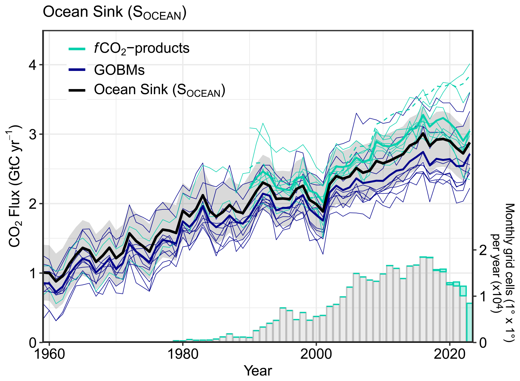
Figure 11 Comparison of the anthropogenic atmosphere–ocean CO₂ flux showing the budget values of S_OCEAN (black; with the uncertainty in grey shading), individual ocean models (royal blue), and the ocean fCO₂ products (cyan; with UExP-FFN-U, previously Watson et al. (2020), in a dashed line as it is not used for ensemble mean). Two fCO₂ products (Jena-MLS, LDEO-HPD) extend back to 1959. The fCO₂ products were adjusted for the pre-industrial ocean source of CO₂ from river input to the ocean by subtracting a source of 0.65 GtC yr⁻¹ to make them comparable to S_OCEAN (see Sect. 2.5). The bar plot in the lower right illustrates the number of monthly gridded values in the SOCAT v2024 database (Bakker et al., 2024). Grey bars indicate the number of grid cells in SOCAT v2023, and coloured bars indicate the newly added grid cells in v2024.

The global net air–sea CO₂ flux is a residual of large natural and anthropogenic CO₂ fluxes into and out of the ocean, with distinct regional and seasonal variations (Figs. 6 and S1). Natural fluxes dominate on regional scales but are largely cancelled out when integrated globally (Gruber et al., 2009). Mid-latitudes in all basins and the high-latitude North Atlantic dominate the ocean CO₂ uptake where low temperatures and high wind speeds facilitate CO₂ uptake at the surface (Takahashi et al., 2009). In these regions, formation of mode, intermediate, and deep water masses transports anthropogenic carbon into the ocean interior, thus allowing for continued CO₂ uptake at the surface. Outgassing of natural CO₂ occurs mostly in the tropics, especially in the equatorial upwelling region and to a lesser extent in the North Pacific and polar Southern Ocean, mirroring a well-established understanding of regional patterns of air–sea CO₂ exchange (e.g. Takahashi et al., 2009; Gruber et al., 2009). These patterns are also noticeable in the Surface Ocean CO₂ Atlas (SOCAT) dataset, where an ocean fCO₂ value above the atmospheric level indicates outgassing (Fig. S1). This map further illustrates the data sparsity in the Indian Ocean and the Southern Hemisphere in general.

The largest variability in the ocean sink occurs on decadal timescales (Fig. 11). The ensemble means of GOBMs and fCO₂ products show the same patterns of decadal variability, although with a larger amplitude of variability in the fCO₂ products than in the GOBMs. The ocean sink stagnated in the 1990s and strengthened between the early 2000s and the mid-2010s (Fig. 11; Le Quéré et al., 2007; Landschützer et al., 2015, 2016; DeVries et al., 2017; Hauck et al., 2020; McKinley et al., 2020; Gruber et al., 2023). More recently, the sink seems to have entered a phase of stagnation since 2016, largely in response to large interannual climate variability. Different explanations have been proposed for the decadal variability in the 1990s and 2000s, ranging from the ocean's response to changes in atmospheric wind systems (e.g. Le Quéré et al., 2007; Keppler and Landschützer, 2019), including variations in upper-ocean overturning circulation (DeVries et al., 2017), to the eruption of Mount Pinatubo in the 1990s (McKinley et al., 2020). The main origin of the decadal variability is a matter of debate, with a number of studies initially pointing to the Southern Ocean (see review in Canadell et al., 2021), but contributions from the North Atlantic and North Pacific (Landschützer et al., 2016; DeVries et al., 2019) or from a global signal (McKinley et al., 2020) have also been proposed.

On top of the decadal variability, interannual variability in the ocean carbon sink is driven by climate variability, with a first-order effect from a stronger ocean sink during large El Niño events (e.g. 1997–1998) (Fig. 11; Rödenbeck et al., 2014; Hauck et al., 2020; McKinley et al., 2017) leading to a reduction in CO₂ outgassing from the tropical Pacific. During 2010–2016, the ocean CO₂ sink appears to have intensified in line with the expected increase from atmospheric CO₂ (McKinley et al., 2020). This effect is similar in the fCO₂ products (Fig. 11, ocean sink 2016 minus 2010; GOBMs: +0.42 ± 0.11 GtC yr⁻¹; fCO₂ products: +0.44 GtC yr⁻¹, range 0.18 to 0.72 GtC yr⁻¹). The reduction of −0.18 GtC yr⁻¹ (range −0.41 to −0.03 GtC yr⁻¹) in the ocean CO₂ sink in 2017 is consistent with the return to normal conditions after the El Niño in 2015/16, which caused an enhanced sink in previous years. After an increasing S_OCEAN in 2018 and 2019, the GOBM and fCO₂-product ensemble means suggest a decrease in S_OCEAN, related to the triple La Niña event 2020–2022, followed by a rebound in 2023, linked to the onset of an El Niño event.

Although all individual GOBMs and fCO₂ products fall within the observational constraint, the ensemble means of GOBMs and fCO₂ products (adjusted for the riverine flux) show a mean offset increasing from 0.31 GtC yr⁻¹ in the 1990s to 0.49 GtC yr⁻¹ in the decade 2014–2023 and a slightly lower offset of 0.3 GtC yr⁻¹ in 2023. In this version of the GCB, the S_OCEAN positive trend has diverged over time by a factor of 1.4 since 2002 (GOBMs: 0.25 ± 0.04 GtC yr⁻¹ per decade; fCO₂ products: 0.35 GtC yr⁻¹ per decade (0.17 to 0.79 GtC yr⁻¹ per decade); S_OCEAN: 0.30 GtC yr⁻¹ per decade), but the uncertainty ranges overlap. This divergence is smaller than reported in previous GCB versions because of the updated lower sink estimates by the fCO₂ products for recent years. This also leads to agreement on the trend since 2010 (GOBMs: 0.18 ± 0.06 GtC yr⁻¹ per decade; fCO₂ products: 0.18 GtC yr⁻¹ per decade (−0.36 to 0.73 GtC yr⁻¹ per decade); S_OCEAN: 0.18 GtC yr⁻¹ per decade). A hybrid approach recently constrained the trend of 2000–2022 to 0.42 ± 0.06 GtC yr⁻¹ per decade (Mayot et al., 2024), which aligns with the updated trends of S_OCEAN (0.39 GtC yr⁻¹ per decade) and of the fCO₂ products (0.45 [0.28, 0.84] GtC yr⁻¹ per decade), while the GOBMs result in a lower trend (0.32 ± 0.04 GtC yr⁻¹ per decade) over the same period.

In the current dataset, the discrepancy between the two types of estimates stems from a persistently larger S_OCEAN in the fCO₂ products in the northern extra-tropics that has been the case since around 2002 and an intermittently larger S_OCEAN in the southern extra-tropics in the period 2008–2020 (Fig. 14). Note that the discrepancy in the mean flux, which was located in the Southern Ocean in GCB2022 and earlier, was reduced due to the choice of the regional river flux adjustment (Lacroix et al., 2020, instead of Aumont et al., 2001). This comes at the expense of a discrepancy in the mean S_OCEAN of about 0.2 GtC yr⁻¹ in the tropics. Likely explanations for the discrepancy in the trends and decadal variability in the high latitudes are data sparsity and uneven data distribution (Bushinsky et al., 2019; Gloege et al., 2021; Hauck et al., 2023a; Mayot et al., 2024). In particular, two fCO₂ products were shown to overestimate the Southern Ocean CO₂ flux trend by 50 % and 130 % based on current sampling in a model subsampling experiment (Hauck et al., 2023a), and the largest trends in the fCO₂ products occurred in a data-void region in the North Pacific (Mayot et al., 2024). In this respect it is highly worrisome that the coverage of fCO₂ observations continues to decline (Dong et al., 2024b) and is now down to that of the early 2000s (Fig. 11). Another likely contributor to the discrepancy between GOBMs and fCO₂ products constitutes model biases (as indicated by the comparison with Mayot et al. (2024); by the large model spread in the south, Fig. 14; and the larger model–data fCO₂ mismatch, Fig. S2).

The reported S_OCEAN estimate from GOBMs and fCO₂ products is 2.2 ± 0.4 GtC yr⁻¹ over the period 1994 to 2007, which is in agreement with the ocean interior estimate of 2.2 ± 0.4 GtC yr⁻¹, which in turn accounts for the climate effect on the natural CO₂ flux of −0.4 ± 0.24 GtC yr⁻¹ (Gruber et al., 2019) to match the definition of S_OCEAN used here (Hauck et al., 2020). This comparison depends critically on the estimate of the climate effect on the natural CO₂ flux, which is smaller from the GOBMs (−0.1 GtC yr⁻¹) than in Gruber et al. (2019). Uncertainties in these two estimates would also overlap when using the GOBM estimate of the climate effect on the natural CO₂ flux. Similarly, the S_OCEAN estimates integrated over the decades 1994–2004 (21.5 GtC yr⁻¹) and 2004–2014 (25.6 GtC yr⁻¹) agree with the interior-ocean-based estimates of Müller et al. (2023; 21.4 ± 2.8 and 26.5 ± 1.3 GtC yr⁻¹) but depend critically on assumptions of the climate effect on natural carbon, which, in turn, are based on the fCO₂ products in Müller et al. (2023).

3.6.3 Final year 2023

The estimated ocean CO₂ sink is 2.9 ± 0.4 GtC for 2023. This is a small increase of 0.16 GtC compared to 2022, in line with the expected sink strengthening from the 2023 El Niño conditions. GOBM and fCO₂-product ensemble mean estimates consistently result in an S_OCEAN increase in 2023 (GOBMs: 0.17 ± 0.15 GtC; fCO₂ products: 0.14 [−0.04, 0.30] GtC). Eight GOBMs and six fCO₂ products show an increase in S_OCEAN, while only two GOBMs and two fCO₂ products show a minor decrease in S_OCEAN of less than 0.05 GtC (Fig. 11). The fCO₂ products have a larger uncertainty at the end of the reconstructed time series, potentially linked to uncertainties related to fewer available observations in the final year and the shift from La Niña to El Niño (see, for example, Watson et al., 2020; Pérez et al., 2024). Specifically, the fCO₂ products' estimate of the last year is regularly adjusted in the following release owing to the tail effect and incrementally increasing data availability. While the monthly grid cells covered may have a lag of only about a year (Fig. 11, lower right), the values within grid cells may change with a 1–5-year lag (see absolute number of observations plotted in previous GCB releases), potentially resulting in annual changes in the flux magnitude from fCO₂ products.

3.6.4 Year 2024 projection

Using a feed-forward neural network method (see Sect. 2.5.2), we project an ocean sink of 3.0 GtC for 2024, only 0.1 GtC higher than for the year 2023 and consistent with El Niño to neutral conditions in 2024. The set of ESM predictions supports this estimate with a 2024 ocean sink of around 3.0 [2.9, 3.1] GtC.

3.6.5 Evaluation of ocean models and fCO₂ products

The process-based model evaluation draws a generally positive picture, with GOBMs scattered around the observational values for Southern Ocean sea-surface salinity, the Southern Ocean stratification index, and the surface ocean Revelle factor (Sect. S3.3 and Table S11). However, the Atlantic Meridional Overturning Circulation at 26° N is underestimated by 8 out of 10 GOBMs and overestimated by 1 GOBM. It is planned to derive skill scores for the GOBMs in future releases based on these metrics.

The model simulations allow us to separate the anthropogenic carbon component (steady-state and non-steady-state, sim D − sim A) and to compare the model flux and dissolved inorganic carbon (DIC) inventory change directly to the interior-ocean estimate of Gruber et al. (2019) without further assumptions (Table S11). The GOBM ensemble average of anthropogenic carbon inventory changes in 1994–2007 amounts to 2.4 GtC yr⁻¹ and is thus lower than the 2.6 ± 0.3 GtC yr⁻¹ estimated by Gruber et al. (2019) although within the uncertainty. Only three models fall within the range reported by Gruber et al. (2019). This suggests that the majority of the GOBMs may underestimate anthropogenic carbon uptake by 10 %–20 % and some models even more. Comparison to the decadal estimates of anthropogenic carbon accumulation (Müller et al., 2023) are close to the estimate based on interior-ocean data for the decade 2004–2014 (GOBMs, sim D minus sim A, 24.7 ± 3.6 GtC yr⁻¹; Müller et al. (2023), 27.3 ± 2.5 GtC yr⁻¹), but they do not reproduce the supposedly higher anthropogenic carbon accumulation in the earlier period 1994–2004 (GOBMs, sim D minus sim A, 21.1 ± 3.0 GtC yr⁻¹; Müller et al. (2023), 29.3 ± 2.5 GtC yr⁻¹). Analysis of Earth system models indicates that an underestimation by about 10 % may be due to biases in ocean carbon transport and mixing from the surface mixed layer to the ocean interior (Goris et al., 2018; Terhaar et al., 2021; Bourgeois et al., 2022; Terhaar et al., 2022), biases in the chemical buffer capacity (Revelle factor) of the ocean (Vaittinada Ayar et al., 2022; Terhaar et al., 2022), and partly a late starting date of the simulations (mirrored in atmospheric CO₂ chosen for the pre-industrial control simulation, Table S2; Bronselaer et al., 2017; Terhaar et al., 2022, 2024). Interestingly, and in contrast to the uncertainties in the surface CO₂ flux, we find the largest mismatch in interior-ocean carbon accumulation in the tropics, with smaller contributions from the north and the south. The large discrepancy in accumulation in the tropics highlights the role of interior-ocean carbon redistribution for those inventories (Khatiwala et al., 2009; DeVries et al., 2023).

The evaluation of the ocean estimates with the fCO₂ observations from the SOCAT v2024 dataset for the period 1990–2023 shows an RMSE from annually detrended data of 0.2 to 2.4 µatm for the eight fCO₂ products over the globe (Fig. S2). The GOBM RMSEs are larger and range from 2.7 to 4.9 µatm. The RMSEs are generally larger at high latitudes compared to the tropics for both the fCO₂ products and the GOBMs. The fCO₂ products have RMSEs of 0.3 to 2.9 µatm in the tropics, 0.6 to 2.4 µatm in the north, and 0.8 to 2.4 µatm in the south. Note that the fCO₂ products are based on the SOCAT v2024 database; hence SOCAT is not an independent dataset for the evaluation of the fCO₂ products. The GOBM RMSEs are more spread across regions, ranging from 2.4 to 3.9 µatm in the tropics, 2.8 to 5.9 µatm in the north, and 2.7 to 6.0 µatm in the south. The higher RMSEs occur in regions with stronger climate variability, such as the northern and southern high latitudes (polewards of the subtropical gyres). Additionally, this year we evaluate the trends derived from a subset of fCO₂ products by subsampling four GOBMs used in Friedlingstein et al. (2023; covering the period up to the year 2022) following the approach of Hauck et al. (2023a) and evaluating the air–sea CO₂ flux trend for the 2001–2021 period, i.e. the period of strong divergence in the air–sea CO₂ exchange excluding the final year to remove the tail effect, against trend biases identified by the GOBM reconstruction. The results indicate a relationship between reconstruction bias and the strength of the decadal trends (see Fig. S3), indicating a tendency of the fCO₂-product ensemble to overestimate the air–sea CO₂ flux trends, in agreement with a recent study by Mayot et al. (2024).

3.7 Land sink

3.7.1 Historical period 1850–2023

Cumulated since 1850, the terrestrial carbon sink amounts to 220 ± 60 GtC, 31 % of total anthropogenic emissions, with more than two-thirds of this amount (150 ± 40 GtC) being taken up by the terrestrial ecosystems since 1960. Over the historical period, the land sink increased in pace with the anthropogenic emissions exponential increase (Fig. 3).

3.7.2 Recent period 1960–2023

The terrestrial CO₂ sink S_LAND increased from 1.2 ± 0.5 GtC yr⁻¹ in the 1960s to 3.2 ± 0.9 GtC yr⁻¹ during 2014–2023, with important interannual variations of up to 2 GtC yr⁻¹ generally showing a decreased land sink during El Niño events (Fig. 9) that is responsible for the corresponding enhanced growth rate in atmospheric CO₂ concentration. The larger land CO₂ sink during 2014–2023 compared to the 1960s is reproduced by all the DGVMs in response to the increase in both atmospheric CO₂ and nitrogen deposition and the changes in climate, and it is consistent with the residual estimated from the other budget terms ($E_{\mathrm{FOS}}+E_{\mathrm{LUC}}-G_{\mathrm{ATM}}-S_{\mathrm{OCEAN}}$, Table 5).

Over the period of 1960 to the present, the increase in the global terrestrial CO₂ sink is largely attributed to the CO₂ fertilization effect (Prentice et al., 2001; Piao et al., 2009; Schimel et al., 2015) and increased nitrogen deposition (Huntzinger et al., 2017; O'Sullivan et al., 2019), directly stimulating plant photosynthesis and increased plant water use in water-limited systems with a small negative contribution of climate change (Fig. 12). There is a range of evidence to support a positive terrestrial carbon sink in response to increasing atmospheric CO₂, albeit with uncertain magnitude (Walker et al., 2021). As expected from theory, the greatest CO₂ effect is simulated in the tropical forest regions, associated with warm temperatures and long growing seasons (Hickler et al., 2008) (Fig. 12a). However, evidence from tropical intact forest plots indicates an overall decline in the land sink across Amazonia (1985–2011), attributed to enhanced mortality offsetting productivity gains (Brienen et al., 2015; Hubau et al., 2020). During 2014–2023 the land sink is positive in all regions (Fig. 6) with the exception of eastern Brazil, Bolivia, northern Venezuela, the southwestern USA, central Europe and Central Asia, northern and southern Africa, and eastern Australia, where the negative effects of climate variability and change (i.e. reduced rainfall and/or increased temperature) counterbalance CO₂ effects. This is clearly visible in Fig. 12, where the effects of CO₂ (Fig. 12a) and climate (Fig. 12b) as simulated by the DGVMs are isolated. The negative effect of climate can be seen across the globe and is particularly strong in most of South America, Central America, the southwestern USA, central Europe, the western Sahel, southern Africa, Southeast Asia and southern China, and eastern Australia (Fig. 12b). Globally, over the 2014–2023 period, climate change reduces the land sink by 0.87 ± 0.56 GtC yr⁻¹ (27 % of S_LAND).

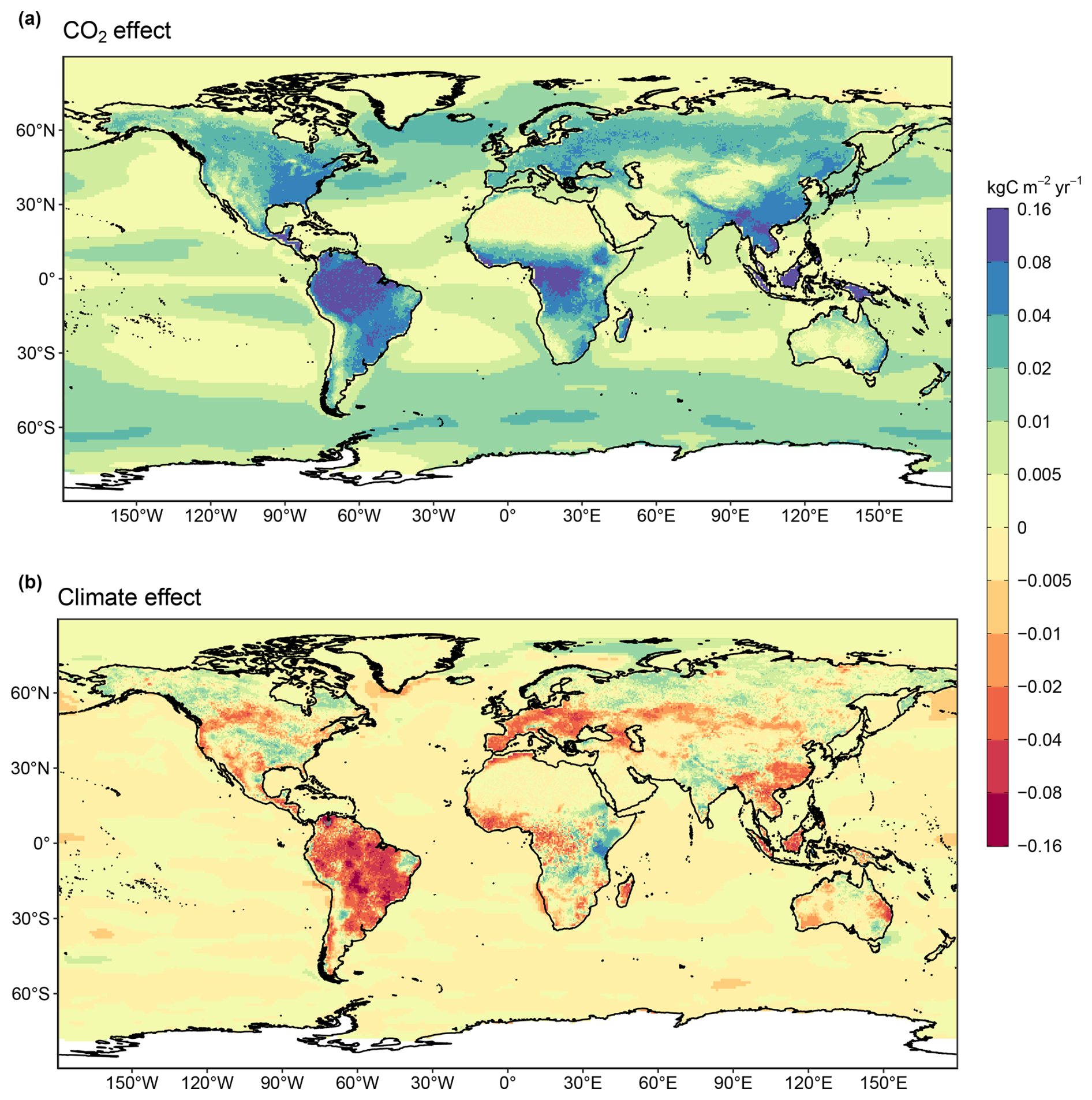
Figure 12 Attribution of the atmosphere–ocean (S_OCEAN) and atmosphere–land (S_LAND) CO₂ fluxes to (a) increasing atmospheric CO₂ concentrations and (b) changes in climate, averaged over the previous decade 2014–2023. All data shown are from the processed-based GOBMs and DGVMs. Note that the sum of ocean CO₂ and climate effects shown here will not equal the ocean sink shown in Fig. 6, which includes the fCO₂ products. See the Supplement, Sects. S3.2 and S4.1, for the attribution methodology. Units are in kgC m⁻² yr⁻¹ (note the non-linear colour scale). Positive values (blue) are CO₂ sinks; negative values (red) are CO₂ sources.

Most DGVMs have similar S_LAND values averaged over 2014–2023: 14 out of 20 models fall within the 1σ range of the residual land sink (1.8–3.7 GtC yr⁻¹) (see Table 5), and all models but 1 are within the 2σ range (0.8–4.6 GtC yr⁻¹). The ED model is an outlier, with a land sink estimate of 5.1 GtC yr⁻¹ for the 2014–2023 period, driven by a strong CO₂ fertilization effect (6.3 GtC yr⁻¹ in the CO₂-only (S1) simulation). There are no direct global observations of the land sink (S_LAND) or the CO₂ fertilization effect, and so we are not yet in a position to rule out models based on component fluxes if their net land sink (S_LAND−E_LUC) is within the observational uncertainty provided by atmospheric inversions or O₂ measurements (Table 5). Furthermore, DGVMs were compared against an analysis based on model–data fusion of the land carbon cycle (CARDAMOM) (Bloom and Williams, 2015; Bloom et al., 2016). Results suggest good correspondence between approaches at interannual timescales but divergence in the recent trend in S_LAND, with CARDAMOM simulating a stronger trend than the DGVM multi-model mean (Fig. 9).

Since 2020 the globe has experienced La Niña conditions, which would be expected to lead to an increased land carbon sink. This 3-year-long period of La Niña conditions came to an end by the second half of 2023 and transitioned to an El Niño that lasted until mid-2024. A clear transition from a maximum to a minimum in the global land sink is evident in S_LAND from 2022 to 2023, and we find that an El Niño-driven decrease in the tropical land sink is offset by a smaller increase in the high-latitude land sink. In the past years, several regions have experienced record-setting fire events (see also Sect. 3.8.3). While the global burned area has declined over the past decades mostly due to declining fire activity in savannas (Andela et al., 2017), forest fire emissions are rising and have the potential to counter the negative fire trend in savannas (Zheng et al., 2021). Noteworthy extreme fire events include the 2019–2020 Black Summer event in Australia (emissions of roughly 0.2 GtC; van der Velde et al., 2021); fires in Siberia in 2021, where emissions approached 0.4 GtC or 3 times the 1997–2020 average according to GFED4.1s; and fires in Canada in 2023 (Byrne et al., 2024a). While other regions, including the western USA and Mediterranean Europe, also experienced intense fire seasons in 2021, their emissions are substantially lower.

Despite these regional negative effects of climate change on S_LAND, the efficiency of land to remove anthropogenic CO₂ emissions has remained broadly constant over the last 6 decades, with a land-borne fraction ($S_{\mathrm{LAND}}/(E_{\mathrm{FOS}}+E_{\mathrm{LUC}}$)) of around 30 % (Fig. 10b).

3.7.3 Final year 2023

The terrestrial CO₂ sink from the DGVM ensemble S_LAND was 2.3 ± 1.0 GtC in 2023, 41 % below the 2022 La Niña-induced strong sink of 3.9 ± 1.0 GtC and also below the 2014–2023 average of 3.2 ± 0.9 GtC yr⁻¹ (Fig. 4, Table 7). We estimate that the 2023 land sink was the lowest since 2015. The severe reduction in the land sink in 2023 is likely driven by the El Niño conditions, leading to a 58 % reduction in S_LAND in the tropics (30° N–30° S) from 2.8 GtC in 2022 to 1.2 GtC in 2023. This is combined with intense wildfires in Canada that led to a significant CO₂ source (see also Sect. 3.8.3). We note that the S_LAND DGVM estimate for 2023 of 2.3 ± 1.0 GtC is very similar to the 2.2 ± 1.0 GtC yr⁻¹ estimate from the residual sink from the global budget ($E_{\mathrm{FOS}}+E_{\mathrm{LUC}}-G_{\mathrm{ATM}}-S_{\mathrm{OCEAN}}$, Table 5).

3.7.4 Year 2024 projection

Using a feed-forward neural network method, we project a land sink of 3.2 GtC for 2024, 0.9 GtC larger than the 2023 estimate. As for the ocean sink, we attribute this to the transition from the El Niño conditions in 2023 to a neutral state. The ESMs do not provide an additional estimate of S_LAND as they only simulate the net atmosphere–land carbon flux (S_LAND−E_LUC).

3.7.5 Evaluation of land models

The evaluation of the DGVMs shows generally higher agreement across models for runoff and to a lesser extent for gross primary production (GPP) and ecosystem respiration. These conclusions are supported by a more comprehensive analysis of DGVM performance in comparison with benchmark data (Sitch et al., 2024). A relative comparison of DGVM performance (Fig. S4) suggests several DGVMs (CABLE-POP, CLASSIC, OCN, ORCHIDEE) may outperform others in terms of multiple carbon and water cycle benchmarks. However, results from Seiler et al. (2022) also show how DGVM differences are often of similar magnitude compared with the range across observational datasets. All models score high enough over the metrics tests to support their use here. There are a few anomalously low scores for individual metrics from a single model, and these can direct the effort to improve models for use in future budgets.

3.8 Partitioning the carbon sinks

3.8.1 Global sinks and spread of estimates

In the period 2014–2023, the bottom-up view of global net ocean and land carbon sinks provided by the GCB, S_OCEAN for the ocean and S_LAND−E_LUC for the land, agrees closely with the top-down global carbon sinks delivered by the atmospheric inversions. This is shown in Fig. 13, which visualizes the individual decadal mean atmosphere–land and atmosphere–ocean fluxes from each, along with the constraints on their sum offered by the global fossil CO₂ emissions flux minus the atmospheric growth rate (E_FOS−G_ATM, 4.4 ± 0.5 GtC yr⁻¹, Table 7, shown as diagonal line in Fig. 13). The GCB estimate for net atmosphere-to-surface flux ($S_{\mathrm{OCEAN}}+S_{\mathrm{LAND}}-E_{\mathrm{LUC}}$) during 2014–2023 is 4.9 ± 1.2 GtC yr⁻¹ (Table 7), with the difference from the diagonal representing the budget imbalance (B_IM) of 0.4 GtC yr⁻¹, discussed in Sect. 3.9. By virtue of the inversion methodology, the atmospheric inversion estimate of the net atmosphere-to-surface flux during 2014–2023 is 4.5 GtC yr⁻¹, with a < 0.1 GtC yr⁻¹ imbalance and thus scatter across the diagonal, with inverse models trading land for ocean fluxes in their solution. The independent constraint on the net atmosphere-to-surface flux based on atmospheric O₂ by design also closes the balance and is 4.5 ± 0.9 GtC yr⁻¹ over the 2014–2023 period (orange symbol in Fig. 13), while the ESM estimate for the net atmosphere-to-surface flux over that period averages to 4.7 [3.0, 5.8] GtC yr⁻¹ (Tables 5 and 6).

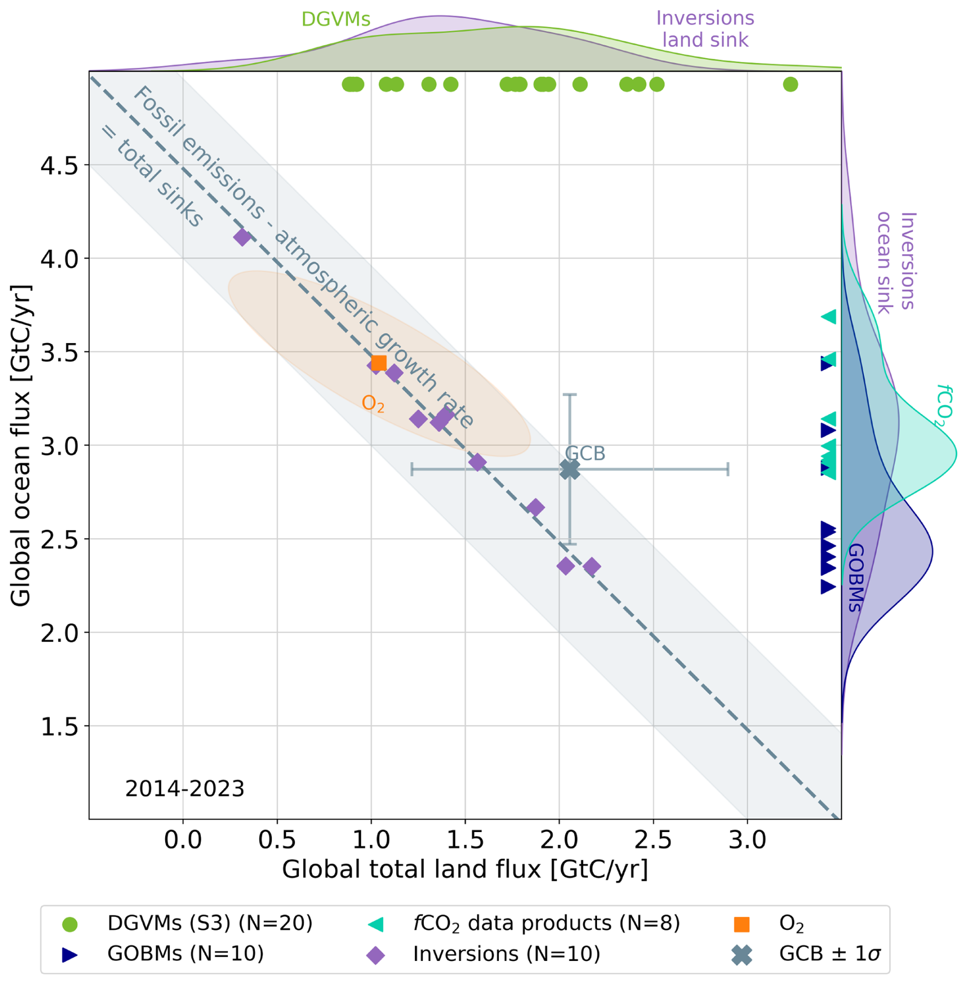
Figure 13 The 2014–2023 decadal mean global net atmosphere–ocean and atmosphere–land fluxes derived from the ocean models and fCO₂ products (y axis, right- and left-pointing blue triangles, respectively) and from the DGVMs (x axis, green symbols), and the same fluxes estimated from the atmospheric inversions (purple symbols). The shaded distributions show the densities of the ensembles of individual estimates. The grey central cross is the mean (±1σ) of S_OCEAN and S_LAND − E_LUC as assessed in this budget. The diagonal grey line represents the constraint on the global land + ocean net flux, i.e. global fossil fuel emissions minus the atmospheric growth rate from this budget (E_FOS − G_ATM). The orange square represents the same global net atmosphere–ocean and atmosphere–land fluxes as estimated from the atmospheric O₂ constraint (the ellipse drawn around the central atmospheric O₂ estimate is a contour representing the 1σ uncertainty in the land and ocean fluxes as a joint probability distribution). Positive values are CO₂ sinks. Note that the inverse estimates have been scaled for a minor difference between E_FOS and GridFEDv2024.0 (Jones et al., 2024a).

The distributions based on the individual models and fCO₂ products reveal substantial spread but converge near the decadal means quoted in Tables 5 to 7. Sink estimates for S_OCEAN and from inverse systems are mostly non-Gaussian, while the ensemble of DGVMs appears more normally distributed, justifying the use of a multi-model mean and standard deviation for their errors in the budget. Noteworthy is that the tails of the distributions provided by the land and ocean bottom-up estimates would not agree with the global constraint provided by the fossil fuel emissions and the observed atmospheric CO₂ growth rate. This illustrates the power of the atmospheric joint constraint from G_ATM and the global CO₂ observation network it is derived from.

Net atmosphere-to-land flux

The GCB estimate of the net atmosphere-to-land flux (S_LAND−E_LUC), calculated as the difference between S_LAND from the DGVMs and E_LUC from the bookkeeping models, amounts to a 2.1 ± 1.1 GtC yr⁻¹ sink during 2014–2023 (Table 5). Estimates of net atmosphere-to-land flux (S_LAND−E_LUC) from the DGVMs alone (1.7 ± 0.6 GtC yr⁻¹, Table 5, green symbols in Fig. 13) are slightly lower, although within the uncertainty in the GCB estimate and also within uncertainty in the global carbon budget constraint ($E_{\mathrm{FOS}}-G_{\mathrm{ATM}}-S_{\mathrm{OCEAN}}$, 1.6 ± 0.6 GtC yr⁻¹, Table 7). Also, for 2014–2023, the inversions estimate that the net atmosphere-to-land flux is a 1.4 [0.3, 2.2] GtC yr⁻¹ sink, slightly lower than the mean of the DGVM estimates (purple versus green symbols in Fig. 13). The independent constraint based on atmospheric O₂ is even lower, 1.0 ± 0.8 GtC yr⁻¹ (orange symbol in Fig. 13), although its large uncertainty overlaps with the uncertainty range from other approaches. Lastly, the ESM estimate for the net atmosphere-to-land flux during 2014–2023 is a 2.2 [0.3, 3.6] GtC yr⁻¹ sink, more consistent with the GCB estimates of S_LAND−E_LUC (Fig. 14, top row).

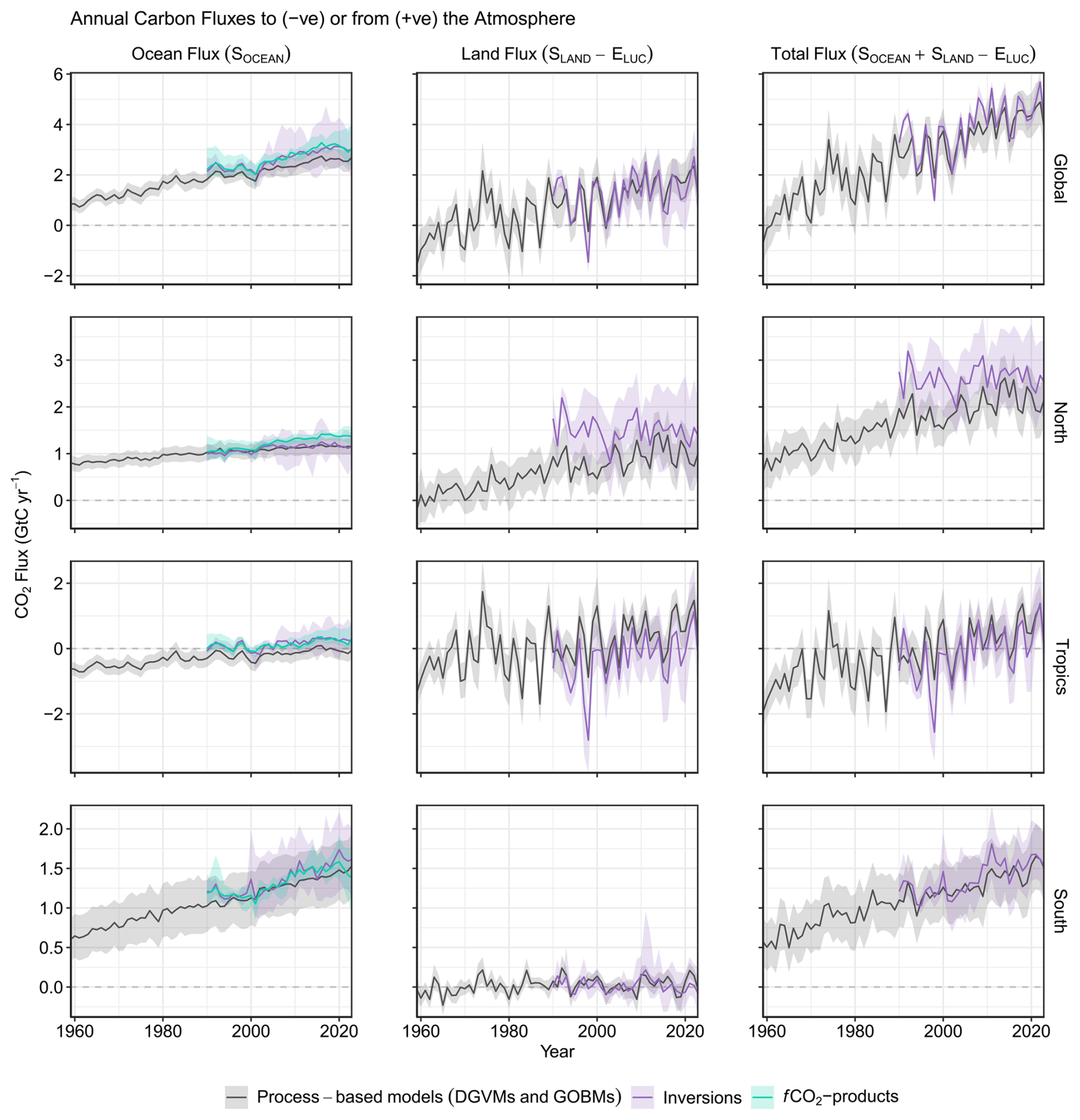
Figure 14 CO₂ fluxes between the atmosphere and the Earth's surface separated between land and oceans, globally and in three latitude bands. The ocean flux is S_OCEAN, and the land flux is the net atmosphere–land fluxes from the DGVMs. The latitude bands are (top row) global, (second row) north (> 30° N), (third row) tropics (30° S–30° N), and (bottom row) south (< 30° S), and the surface categories are over ocean (left column), over land (middle column), and total (right column). Estimates are shown for process-based models (DGVMs for land, GOBMs for oceans), inversion systems (land and ocean), and fCO₂ products (ocean only). Positive values are CO₂ sinks. Mean estimates from the combination of the process models for the land and oceans are shown (black line) with ±1σ of the model ensemble (grey shading). For the total uncertainty in the process-based estimate of the total sink, uncertainties are summed in quadrature. Mean estimates from the atmospheric inversions are shown (purple lines) with their full spread (purple shading). Mean estimates from the fCO₂ products are shown for the ocean domain (light-blue lines) with full model spread (light-blue shading). The global S_OCEAN (upper left) and the sum of S_OCEAN in all three regions represent the anthropogenic atmosphere-to-ocean flux based on the assumption that the pre-industrial ocean sink was 0 GtC yr⁻¹ when riverine fluxes are not considered. This assumption does not hold at the regional level, where pre-industrial fluxes can be significantly different from zero. Hence, the regional panels for S_OCEAN represent a combination of natural and anthropogenic fluxes. Bias correction and area weighting were only applied to global S_OCEAN; hence the sum of the regions is slightly different from the global estimate (< 0.07 GtC yr⁻¹).

As discussed in Sect. 3.5.3, the atmospheric growth rate of CO₂ was very high in 2023, 5.9 GtC (2.79 ppm) the fourth largest on record. Both DGVMs and inversions assign this large CO₂ growth rate to a severe decrease in the net atmosphere-to-land flux, in particular in the tropics (Fig. 14). DGVMs simulate a 2023 global net atmosphere-to-land flux of 1.1 GtC yr⁻¹, a 55 % decline relative to the 2.4 GtC yr⁻¹ sink in 2022, primarily driven by the severe reduction in S_LAND (−41 %; see Sect. 3.7.3). The tropics (30° N–30° S) are recording a dramatic decrease in the net atmosphere-to-land flux from 1.5 GtC yr⁻¹ in 2022 to 0.1 GtC yr⁻¹ in 2023. The atmospheric inversion shows a similar story, with the global net atmosphere-to-land flux declining from 2.6 GtC yr⁻¹ in 2022 to 0.9 GtC yr⁻¹ in 2023 (−64 %) and the tropics turning from a 1.0 GtC yr⁻¹ sink in 2022 to a 0.4 GtC yr⁻¹ source in 2023. Our results are broadly consistent with the Ke et al. (2024) study, which reported a global atmosphere-to-land flux of 0.4 ± 0.2 GtC yr⁻¹ in 2023.

In addition to the large decline in the tropical land uptake, the northern extra-tropics experienced warmer-than-average conditions, in particular in the summer over North America and northern Eurasia. In Canada alone, 2023 led to enhanced CO₂ release due to fires of 0.5–0.8 GtC yr⁻¹ (see Sect. 3.8.3). The atmospheric inversions do simulate a slight reduction in the atmosphere-to-land flux in the northern extra-tropics (north of 30° N), from 1.6 GtC yr⁻¹ in 2022 to 1.4 GtC yr⁻¹ in 2023, while the DGVMs fail to capture this pattern, with a simulated northern extra-tropics net atmosphere-to-land flux larger in 2023 than in 2022 (1.0 vs. 0.7 GtC yr⁻¹).

Net atmosphere-to-ocean flux

For the 2014–2023 period, the GOBMs (2.6 ± 0.4 GtC yr⁻¹) produce a lower estimate for S_OCEAN than the fCO₂ products, with 3.1 [2.9, 3.7] GtC yr⁻¹, which shows up in Fig. 13 as separate peaks in the distribution from the GOBMs (dark-blue symbols) and from the fCO₂ products (light-blue symbols). Atmospheric inversions (3.1 [2.4, 4.1] GtC yr⁻¹) suggest an ocean uptake more in line with the fCO₂ products for the recent decade (Table 7), although the inversions' range includes both the GOBM and the fCO₂-product estimates (Fig. 14, top row) and the inversions are not fully independent as 6 out of 10 inversions covering the last decade use fCO₂ products as ocean priors and one uses a GOBM (Table S4). The independent constraint based on atmospheric O₂ (3.4 ± 0.5 GtC yr⁻¹) is at the high end of the distribution of the other methods. However, as mentioned in Sect. 2.8, the O₂ method requires a correction for global air–sea O₂ flux, which induces a non-negligible uncertainty in the decadal estimates (about 0.5 GtC yr⁻¹). The large growth in the ocean carbon sink from O₂ is compatible with the GOBM and fCO₂-product estimates when accounting for their uncertainty ranges. Lastly, the ESM estimate, 2.5 [2.2, 2.8] GtC yr⁻¹, suggests a moderate ocean carbon sink, comparable to the GOBM estimate with regard to mean and spread. We caution that the riverine transport of carbon taken up on land and outgassing from the ocean, accounted for here, is a substantial (0.65 ± 0.3 GtC yr⁻¹) and uncertain term (Crisp et al., 2022; Gruber et al., 2023; DeVries et al., 2023) that separates the GOBM, ESM, and oxygen-based estimates on the one hand from the fCO₂ products and atmospheric inversions on the other hand.

3.8.2 Regional partitioning

Figure 14 shows the latitudinal partitioning of the global atmosphere-to-ocean flux (S_OCEAN) and atmosphere-to-land flux (S_LAND−E_LUC) and their sum ($S_{\mathrm{OCEAN}}+S_{\mathrm{LAND}}-E_{\mathrm{LUC}}$) according to the estimates from GOBMs and ocean fCO₂ products (S_OCEAN), DGVMs (S_LAND−E_LUC), and atmospheric inversions (S_OCEAN and S_LAND−E_LUC).

North

Despite being one of the most densely observed and studied regions of our globe, annual mean carbon sink estimates in the northern extra-tropics (north of 30° N) continue to differ. The atmospheric inversions suggest an atmosphere-to-surface sink ($S_{\mathrm{OCEAN}}+S_{\mathrm{LAND}}-E_{\mathrm{LUC}}$) for 2014–2023 of 2.6 [2.0, 3.4] GtC yr⁻¹, which is slightly higher than the process models' estimate of 2.2 ± 0.4 GtC yr⁻¹ (Fig. 14). The GOBMs (1.2 ± 0.2 GtC yr⁻¹), fCO₂ products (1.4 [1.3, 1.5] GtC yr⁻¹), and inversion systems (1.2 [0.9, 1.4] GtC yr⁻¹) produce largely consistent estimates of the ocean sink. However, the larger flux in the fCO₂ products may be related to data sparsity (Mayot et al., 2024). Thus, the difference mainly arises from the net land flux (S_LAND−E_LUC) estimate, which is 1.0±0.4 GtC yr⁻¹ in the DGVMs compared to 1.5 [0.6, 2.3] GtC yr⁻¹ in the atmospheric inversions (Fig. 14, second row).

Discrepancies in the northern land fluxes conform with persistent issues surrounding the quantification of the drivers of the global net land CO₂ flux (Arneth et al., 2017; Huntzinger et al., 2017; O'Sullivan et al., 2022) and the distribution of atmosphere-to-land fluxes between the tropics and high northern latitudes (Baccini et al., 2017; Schimel et al., 2015; Stephens et al., 2007; Ciais et al., 2019; Gaubert et al., 2019).

In the northern extra-tropics, the process models, inversions, and fCO₂ products consistently suggest that most of the interannual variability stems from the land (Fig. 14). Inversions generally agree on the magnitude of interannual variations (IAVs) over land, more so than DGVMs (0.29–0.32 vs. 0.14–0.63 GtC yr⁻¹, averaged over 1990–2023).

Tropics

In the tropics (30° S–30° N), both the atmospheric inversions and the process models estimate a net carbon balance ($S_{\mathrm{OCEAN}}+S_{\mathrm{LAND}}-E_{\mathrm{LUC}}$) that has been relatively close to neutral over the past decade (inversions: 0.3 [−0.4, 0.9] GtC yr⁻¹; process models: 0.6±0.6 GtC yr⁻¹). The GOBMs (−0.03 ± 0.3 GtC yr⁻¹), fCO₂ products (0.3 [0.1, 0.6] GtC yr⁻¹), and inversion systems (0.3 [−0.1, 0.8] GtC yr⁻¹) indicate a neutral to positive tropical ocean flux (see Fig. S1 for spatial patterns). DGVMs indicate a net land sink (S_LAND−E_LUC) of 0.6 ± 0.4 GtC yr⁻¹, whereas the inversion systems indicate a neutral net land flux although with large model spread (−0.0 [−0.9, 0.8] GtC yr⁻¹, Fig. 14, third row).

The tropical lands are the origin of most of the atmospheric CO₂ interannual variability (Ahlström et al., 2015) consistently among the process models and inversions (Fig. 14). The interannual variability in the tropics is similar among the ocean fCO₂ products (0.06–0.16 GtC yr⁻¹) and the GOBMs (0.07–0.16 GtC yr⁻¹, Fig. S2). The DGVMs and inversions indicate that atmosphere-to-land CO₂ fluxes are more variable than atmosphere-to-ocean CO₂ fluxes in the tropics, with interannual variability of 0.37–1.33 and 0.86–0.96 GtC yr⁻¹ for DGVMs and inversions, respectively.

South

In the southern extra-tropics (south of 30° S), the atmospheric inversions suggest a net atmosphere-to-surface sink ($S_{\mathrm{OCEAN}}+S_{\mathrm{LAND}}-E_{\mathrm{LUC}}$) for 2014–2023 of 1.5 [1.2, 1.9] GtC yr⁻¹, identical to the process models' estimate of 1.5 ± 0.4 GtC yr⁻¹ (Fig. 14). An approximately neutral net land flux (S_LAND−E_LUC) for the southern extra-tropics is estimated by both the DGVMs (0.05 ± 0.1 GtC yr⁻¹) and the inversion systems (−0.03 [−0.11, 0.08] GtC yr⁻¹). This means nearly all carbon uptake is due to oceanic sinks south of 30° S. The Southern Ocean flux in the fCO₂ products (1.5 [1.3, 1.7] GtC yr⁻¹) and inversion estimates (1.6 [1.2, 1.9] GtC yr⁻¹) is marginally higher than in the GOBMs (1.4 ± 0.4 GtC yr⁻¹) (Fig. 14, bottom row). This agreement is subject to the choice of the river flux adjustment (Lacroix et al., 2020; Hauck et al., 2023b). Nevertheless, the time series of atmospheric inversions and fCO₂ products diverge from those of the GOBMs. A substantial overestimation of the trends in the fCO₂ products could be explained by sparse and unevenly distributed observations, especially in wintertime (Fig. S1; Hauck et al., 2023a; Gloege et al., 2021). Model biases may contribute as well, with biases in mode water formation, stratification, and the chemical buffer capacity known to play a role in Earth system models (Terhaar et al., 2021; Bourgeois et al., 2022; Terhaar et al., 2022).

The interannual variability in the southern extra-tropics is low because of the dominance of ocean areas with low variability compared to land areas. The split between land (S_LAND−E_LUC) and ocean (S_OCEAN) shows a substantial contribution to variability in the south coming from the land, with no consistency between the DGVMs and the inversions or among inversions. This is expected due to the difficulty of precisely separating the land and oceanic fluxes when viewed from the perspective of atmospheric observations alone. The S_OCEAN interannual variability was found to be higher in the fCO₂ products (0.04–0.20 GtC yr⁻¹) compared to GOBMs (0.04–0.06 GtC yr⁻¹) in 1990–2023 (Fig. S2). Inversions give an interannual variability of 0.10 to 0.13 GtC yr⁻¹. Model subsampling experiments recently illustrated that fCO₂ products may overestimate decadal variability in the Southern Ocean carbon sink by 30 % and the trend since 2000 by 50 %–130 % due to data sparsity, based on fCO₂ products with strong variability (Gloege et al., 2021; Hauck et al., 2023a). The trend benchmark test using the method of Hauck et al. (2023a) and a subset of six fCO₂ products confirms the sensitivity of the decadal trends in fCO₂ products to reconstruction biases, particularly in the Southern Ocean, indicating an overestimation of the ensemble mean trend. However, we also find compensatory positive biases in the ensemble, so the ensemble mean bias is smaller than the bias from some individual fCO₂ products.

RECCAP-2 regions

Aligning with the RECCAP-2 initiative (Ciais et al., 2022; Poulter et al., 2022; DeVries et al., 2023), we provide a breakdown of this GCB paper estimate of the E_LUC, S_LAND, net land (S_LAND−E_LUC), and S_OCEAN fluxes over the 10 land and 5 ocean RECCAP-2 regions, averaged over the period 2014–2023 (Fig. 15). The DGVMs and inversions suggest a positive net land sink in all regions, except for South America and Africa, where the inversions indicate a small net source of −0.1 [−0.8, 0.3] GtC yr⁻¹ and −0.3 [−0.7, −0.1] GtC yr⁻¹, respectively, compared to a small sink of 0.1 ± 0.3 GtC yr⁻¹ and 0.3 ± 0.1 GtC yr⁻¹ for the DGVMs. However, for South America, there is substantial uncertainty in both products (ensembles span zero). For the DGVMs, this is driven by uncertainty in both S_LAND (0.5 ± 0.4 GtC yr⁻¹) and E_LUC (0.4 ± 0.2 GtC yr⁻¹). The bookkeeping models also suggest an E_LUC source of around 0.4 GtC yr⁻¹ in South America and Africa, in line with the DGVM estimates. Bookkeeping models and DGVMs similarly estimate a source of 0.3–0.4 GtC yr⁻¹ in Southeast Asia, with DGVMs suggesting a small net land sink (0.1 ± 0.1 GtC yr⁻¹). This is similar to the inversion mean estimate of a 0.1 [−0.3, 0.8] GtC yr⁻¹ sink, although the inversion spread is substantial. The inversions suggest the largest net land sinks are located in North America (0.5 [−0.1, 1.0] GtC yr⁻¹), Russia (0.6 [0.1, 0.9] GtC yr⁻¹), and East Asia (0.4 [−0.2, 1.3] GtC yr⁻¹). This agrees well with the DGVMs in North America (0.4 ± 0.1 GtC yr⁻¹), which indicate a large natural land sink (S_LAND) of 0.6 ± 0.2 GtC yr⁻¹, being slightly reduced by land-use-related carbon losses (0.2 ± 0.1 GtC yr⁻¹). The DGVMs suggest a smaller net land sink in Russia compared to inversions (0.3 ± 0.2 GtC yr⁻¹) and a similar net sink in East Asia (0.2 ± 0.1 GtC yr⁻¹).

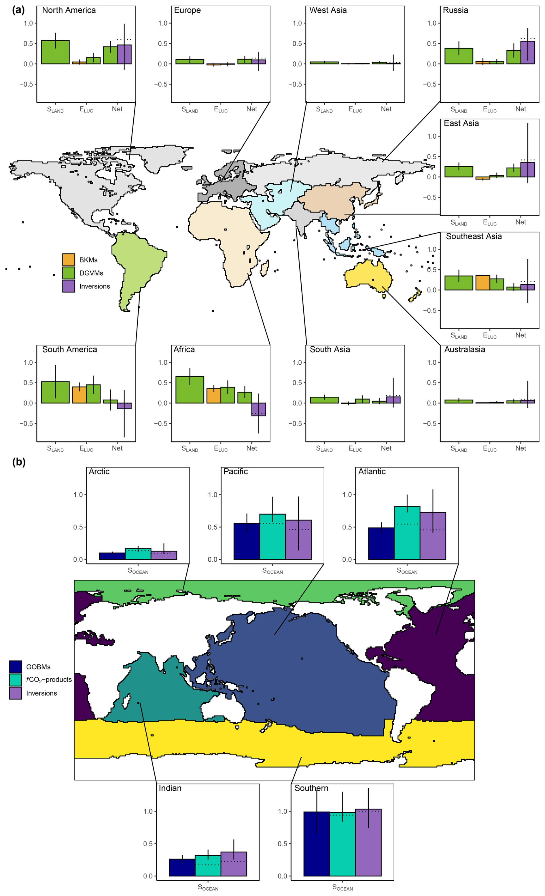
Figure 15 Decadal mean (a) land and (b) ocean fluxes for RECCAP-2 regions over 2014–2023. For land fluxes, S_LAND is estimated by the DGVMs (green bars), with the error bar as ±1σ spread among models. A positive S_LAND is a net transfer of carbon from the atmosphere to the land. E_LUC fluxes are shown for both DGVMs (green) and bookkeeping models (orange), again with the uncertainty calculated as the ±1σ spread. Note that a positive E_LUC flux indicates a loss of carbon from the land. The net land flux is shown for both DGVMs (green) and atmospheric inversions (purple), including the full model spread for inversions. The net ocean sink (S_OCEAN) is estimated by GOBMs (royal blue), fCO₂ products (cyan), and atmospheric inversions (purple). Uncertainty is estimated as the ±1σ spread for GOBMs and as the full model spread for the other two datasets. The dotted lines show the fCO₂ products and inversion results without river flux adjustment. Positive values are CO₂ sinks.

There is generally a higher level of agreement in the estimates of regional S_OCEAN between the different data streams (GOBMs, fCO₂ products, and atmospheric inversions) on a decadal scale compared to the agreement between the different land flux estimates. All data streams agree that the largest contribution to S_OCEAN stems from the Southern Ocean due to a combination of high flux density and large surface area, but with important contributions also from the Atlantic (high flux density) and Pacific (large area) basins. In the Southern Ocean, GOBMs suggest a sink of 1.0 ± 0.3 GtC yr⁻¹, in line with the fCO₂ products (1.0 [0.8, 1.3] GtC yr⁻¹) and atmospheric inversions (1.0 [0.7, 1.4] GtC yr⁻¹). There is similar agreement in the Pacific Ocean, with GOBMs, fCO₂ products, and atmospheric inversions indicating a sink of 0.6 ± 0.2 GtC yr⁻¹, 0.7 [0.6, 1.0] GtC yr⁻¹, and 0.6 [0.1, 1.0] GtC yr⁻¹, respectively. However, in the Atlantic Ocean, GOBMs simulate a sink of 0.5 ± 0.1 GtC yr⁻¹, noticeably lower than both the fCO₂ products (0.8 [0.7, 1.0] GtC yr⁻¹) and atmospheric inversions (0.7 [0.4, 1.1] GtC yr⁻¹). It is important to note the fCO₂ products and atmospheric inversions have a substantial and uncertain river flux adjustment in the Atlantic Ocean (0.3 GtC yr⁻¹) that also leads to a mean offset between GOBMs and fCO₂ products and inversions in the latitude band of the tropics (Fig. 14). The Indian Ocean, due to its smaller size, and the Arctic Ocean, due to its size and sea-ice cover that prevents air–sea gas exchange, are responsible for smaller but non-negligible S_OCEAN fluxes (Indian Ocean: 0.3 [0.2, 0.3] GtC yr⁻¹, 0.3 [0.3, 0.4] GtC yr⁻¹, and 0.4 [0.3, 0.6] GtC yr⁻¹ for GOBMs, fCO₂ products, and atmospheric inversions, respectively; Arctic Ocean: 0.1 [0.1, 0.1] GtC yr⁻¹, 0.2 [0.1, 0.2] GtC yr⁻¹, and 0.1 [0.1, 0.2] GtC yr⁻¹ for GOBMs, fCO₂ products, and atmospheric inversions, respectively). Note that the S_OCEAN numbers presented here deviate from numbers reported in RECCAP-2 where the net air–sea CO₂ flux is reported (i.e. without river flux adjustment for fCO₂ products and inversions and with river flux adjustment subtracted from GOBMs in most chapters or comparing unadjusted datasets with discussion of uncertain regional riverine fluxes as major uncertainty, e.g. Sarma et al., 2023; DeVries et al., 2023).

Tropical vs. northern land uptake

A continuing conundrum is the partitioning of the global atmosphere–land flux between the Northern Hemisphere land and the tropical land (Stephens et al., 2007; Pan et al., 2011; Gaubert et al., 2019). It is of importance because each region has its own history of land-use change, climate drivers, and the impact of increasing atmospheric CO₂ and nitrogen deposition. Quantifying the magnitude of each sink is a prerequisite to understanding how each individual driver impacts the tropical and mid- to high-latitude carbon balance.

We define the north–south (N–S) difference as net atmosphere–land flux north of 30° N minus the net atmosphere–land flux south of 30° N. For the inversions, the N–S difference is 1.50 [0.05, 3.0] GtC yr⁻¹ across this year's inversion ensemble. An apparent clustering of six satellite-driven solutions towards a common NH land sink noted in GCB2023 is no longer clear.

In the ensemble of DGVMs the N–S difference is 0.4 ± 0.5 GtC yr⁻¹, a much narrower range than the one from atmospheric inversions. Only 3 out of 20 DGVMs have a N–S difference larger than 1.0 GtC yr⁻¹, compared to half of the inversion systems simulating a difference at least this large. The smaller spread across DGVMs compared to across inversions is to be expected as there is no correlation between northern and tropical land sinks in the DGVMs as opposed to the inversions where the sum of the two regions being well constrained by atmospheric observations leads to an anti-correlation between these two regions. This atmospheric N–S gradient could be used as an additional way to evaluate tropical and NH uptake in DGVMs if their fluxes were combined with multiple transport models. Vice versa, the much smaller spread in the N–S difference between the DGVMs could help in scrutinizing the inverse systems further. For example, a large northern land sink and a tropical land source in an inversion would suggest large sensitivity to CO₂ fertilization (the dominant factor driving the land sinks) for northern ecosystems, which would not be mirrored by tropical ecosystems. Such a combination could be hard to reconcile with the process understanding gained from the DGVM ensembles and independent measurements (e.g. free-air CO₂ enrichment (FACE) experiments).

3.8.3 Fire emissions in 2024

Fire emissions so far in 2024 have been above the average of recent decades, chiefly due to synchronous large emissions fluxes from North America and South America. Figure S9 shows global and regional emissions estimates for the period of 1 January–30 September in each year 2003–2024. Estimates are derived from two global fire emissions products: the Global Fire Emissions Database (GFED, version 4.1s; van der Werf et al., 2017) and the Global Fire Assimilation System (GFAS, operated by the Copernicus Atmosphere Monitoring Service; Kaiser et al., 2012). The two products estimate that global emissions from fires were 1.6–2.2 GtC yr⁻¹ during January–September 2024. These estimates are 11 %–32 % above the 2014–2023 average for the same months (1.5–1.7 GtC yr⁻¹). In the GFED4.1s product, the year-to-date emissions in 2024 were at their highest since 2003, exceeding even the large emissions estimate of 2023, whereas the GFAS product showed lower emissions in 2024 than in 2023 and in six other years since 2003.

The pattern of high fire emissions from Canada in 2023, which were record-breaking (Jones et al., 2024b; Byrne et al., 2024a), continued into 2024. In January–September 2024, emissions from Canada (0.2–0.3 GtC yr⁻¹) were half as great as in the same months of 2023 (0.5–0.8 GtC yr⁻¹) but still 2.1–2.3 times the average of January–September periods in 2014–2023 (and 4–6 times greater than the average of those months in 2003–2022 (excluding the record-breaking year in 2023); Fig. S9). The continued anomaly in Canada propagated to the Northern Hemisphere, where emissions of 0.5–0.6 GtC yr⁻¹ were 26 %–44 % above the average of 2014–2023.

In January–September 2024, fire emissions from South America (0.4–0.6 GtC yr⁻¹) were 94 %–164 % above the average of the January–September periods in 2014–2023, marking 2024 out as a year with synchronous high fire emissions across the Americas. Emissions from Brazil in January–September 2024 (0.2–0.3 GtC yr⁻¹) were 91 %–118 % above the average of January–September periods of 2014–2023 and were at a level not seen since the major drought year of 2010 (Fig. S9; Aragão et al., 2018; Silva Junior et al., 2019). In 2023, deforestation fire activity in the Brazilian Amazon was below the average levels recorded in national recording systems and is attributed to renewed environmental policy implementation; however the fall in Amazon deforestation fire activity was largely offset by above-average wildfires related to historic drought (Mataveli et al., 2024). According to the National Center for Monitoring and Early Warning of Natural Disasters (CEMADEN), drought conditions continued into 2024 and the current drought is the most intense and widespread that Brazil has experienced since records began in 1950 (CEMADEN, 2024), prompting large wildfire anomalies across the Amazon, Cerrado, and Pantanal regions (INPE, 2024).

Emissions anomalies in Africa strongly influence global totals because the continent typically contributed 41 %–47 % of global fire emissions during 2014–2023 (average of January–September periods). GFAS suggests that fire emissions in Africa through September 2024 (0.6 GtC yr⁻¹) were slightly below the average of 2014–2023, whereas GFED4.1s suggests that fire emissions through September 2024 were slightly above the average of 2014–2023 (0.8 GtC yr⁻¹).

Tropical fire emissions through September 2024 (1.1–1.6 GtC yr⁻¹) accounted for 69 %–74 % of the global total emissions, which is close to the average of the 2014–2023 period (1.1–1.2 GtC yr⁻¹; 72 %–75 %). This marks a return to a more typical distribution of fire emissions between the tropics and extra-tropics after the tropical contribution fell to just 55 %–59 % during January–September 2023 (Fig. S9).

We caution that the fire emissions fluxes presented here should not be compared directly with other fluxes of the budget (e.g. S_LAND or E_LUC) due to incompatibilities between the observable fire emissions fluxes and what is quantified in the S_LAND and E_LUC components of the budget. The fire emissions estimates from global fire products relate to all fire types that can be observed in Earth observations (Giglio et al., 2018; Randerson et al., 2012; Kaiser et al., 2012), including (i) fires occurring as part of natural disturbance–recovery cycles that would also have occurred in the pre-industrial period (Yue et al., 2016; Keeley and Pausas, 2019; Zou et al., 2019); (ii) fires occurring above and beyond natural disturbance–recovery cycle due to changes in climate, CO₂, and N fertilization and to an increased frequency of extreme drought and heatwave events (Abatzoglou et al., 2019; Jones et al., 2022; Zheng et al., 2021; Burton et al., 2024); and (iii) fires occurring in relation to land use and land-use change, such as deforestation fires and agricultural fires (van der Werf et al., 2010; Magi et al., 2012). In the context of the global carbon budget, only the portion of fire emissions associated with (ii) should be included in the S_LAND component, and fire emissions associated with (iii) should already be accounted for in the E_LUC component. Emissions associated with (i) should not be included in the global carbon budget. It is not currently possible to derive specific estimates for fluxes (i), (ii), and (iii) using global fire emissions products such as GFED or GFAS. In addition, the fire emissions estimates from global fire emissions products represent a gross flux of carbon to the atmosphere, whereas the S_LAND component of the budget is a net flux that should also include post-fire recovery fluxes. Even if emissions from fires of type (ii) could be separated from those of type (i), these fluxes may be partially or wholly offset in subsequent years by post-fire fluxes as vegetation recovers, sequestering carbon from the atmosphere to the terrestrial biosphere (Yue et al., 2016; Jones et al., 2024c). Increases in forest fire emissions and severity (emissions per unit area) globally during the past 2 decades have highlighted the increasing potential for fire emissions fluxes to outweigh post-fire recovery fluxes, though long-term monitoring of vegetation recovery is required to quantify the net effect on terrestrial C storage (Jones et al., 2024c).

3.9 Closing the global carbon cycle

3.9.1 Partitioning of cumulative emissions and sink fluxes

Emissions during the period 1850–2023 amounted to 710 ± 70 GtC and were partitioned among the atmosphere (285 ± 5 GtC; 40 %), ocean (185 ± 35 GtC; 26 %), and land (220 ± 60 GtC; 32 %). The cumulative land sink is almost equal to the cumulative land-use emissions (225 ± 65 GtC), making the global land nearly neutral over the whole 1850–2023 period (Fig. 3).

The use of nearly independent estimates for the individual terms of the global carbon budget shows a cumulative budget imbalance of 25 GtC (3 % of total emissions) during 1850–2023 (Fig. 3, Table 8), which, if correct, suggests that emissions could be slightly too high by the same proportion or that the combined land and ocean sinks are slightly underestimated (by about 6 %), although these are well within the uncertainty range of each component of the budget. Nevertheless, part of the imbalance could originate from the estimation of significant increase in E_FOS and E_LUC between the mid-1920s and the mid-1960s which is unmatched by a similar growth in atmospheric CO₂ concentration as recorded in ice cores (Fig. 3). However, the known loss of additional sink capacity of 30–40 GtC (over the 1850–2020 period) due to reduced forest cover has not been accounted for in our method and would exacerbate the budget imbalance (see Sects. 2.10 and S6.4).

For the more recent 1960–2023 period where direct atmospheric CO₂ measurements are available, total emissions (E_FOS+E_LUC) amounted to 500 ± 50 GtC, of which 410 ± 20 GtC (82 %) was caused by fossil CO₂ emissions and 90 ± 45 GtC (18 %) by land-use change (Table 8). The total emissions were partitioned among the atmosphere (220 ± 5 GtC; 45 %), ocean (130 ± 26 GtC; 25 %), and land (150 ± 40 GtC; 30 %), with a near-zero (< 1 GtC) unattributed budget imbalance. All components except land-use change emissions have significantly grown since 1960, with important interannual variability in the growth rate in atmospheric CO₂ concentration and in the land CO₂ sink (Fig. 4) and some decadal variability in all terms (Table 7). Differences with previous budget releases are documented in Fig. S6.

The global carbon budget averaged over the last decade (2014–2023) is shown in Figs. 2 and 16 (right panel) and Table 7. For this period, 90 % of the total emissions (E_FOS+E_LUC) were from fossil CO₂ emissions (E_FOS) and 10 % from land-use change (E_LUC). The total emissions were partitioned among the atmosphere (48 %), ocean (26 %), and land (30 %), with a small negative budget imbalance (∼ 4 %, 0.4 GtC yr⁻¹). For single years, the budget imbalance can be larger (Fig. 4). For 2023, the combination of our estimated sources (11.1 ± 0.9 GtC yr⁻¹) and sinks (11.1 ± 0.9 GtC yr⁻¹) leads to a B_IM of −0.02 GtC, suggesting a near-perfect closure of the global carbon budget.

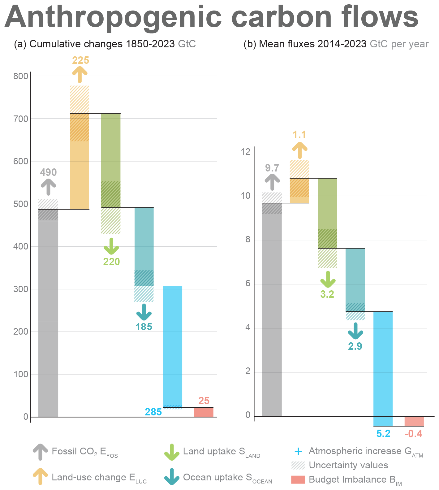
Figure 16 Cumulative changes over the 1850–2023 period (a) and average fluxes over the 2014–2023 period (b) for the anthropogenic perturbation of the global carbon cycle. See the caption of Fig. 3 for key information and the Methods section in the text for full details. This figure was produced by Nigel Hawtin.

3.9.2 Trend and variability in the carbon budget imbalance

The carbon budget imbalance (B_IM; Eq. 1, Fig. 4) quantifies the mismatch between the estimated total emissions and the estimated changes in the atmosphere, land, and ocean reservoirs. The budget imbalance from 1960 to 2023 is very small (0.5 GtC over the period, i.e. < 0.01 GtC yr⁻¹ on average) and shows no trend over the full time series (Fig. 4e). The process models (GOBMs and DGVMs) and fCO₂ products have been selected to match observational constraints in the 1990s, but no further constraints have been applied to their representation of trend and variability. Therefore, the near-zero mean of and trend in the budget imbalance are seen as evidence of a coherent community understanding of the emissions and their partitioning on those timescales (Fig. 4). However, the budget imbalance shows substantial variability on the order of ±1 GtC yr⁻¹, particularly over semi-decadal timescales, although most of the variability is within the uncertainty in the estimates. The positive carbon imbalance during the 1960s and early 1990s indicates that either the emissions were overestimated or the sinks were underestimated during these periods. The reverse is true for the 1970s and to a lesser extent for the 1980s and 2014–2023 period (Fig. 4, Table 7).

We cannot attribute the cause of the variability in the budget imbalance with our analysis; we only note that the budget imbalance is unlikely to be explained by errors or biases in the emissions alone because of its component of large semi-decadal variability, a variability that is atypical of emissions and has not changed in the past 60 years despite a near tripling in emissions (Fig. 4). Errors in S_LAND and S_OCEAN are more likely to be the main cause for the budget imbalance, especially on interannual to semi-decadal timescales. For example, underestimation of the S_LAND by DGVMs has been reported following the eruption of Mount Pinatubo in 1991, possibly due to missing responses to changes in diffuse radiation (Mercado et al., 2009). Although since GCB2021 we have accounted for aerosol effects on solar radiation quantity and quality (diffuse vs. direct), most DGVMs only used the former as input (i.e. total solar radiation) (Table S1). Thus, the ensemble mean may not capture the full effects of volcanic eruptions, i.e. those associated with high-light-scattering sulfate aerosols, on the land carbon sink (O'Sullivan et al., 2021). DGVMs are suspected to overestimate the land sink in response to the wet decade of the 1970s (Sitch et al., 2008). Quasi-decadal variability in the ocean sink has also been reported, with all methods agreeing on a smaller-than-expected ocean CO₂ sink in the 1990s and a larger-than-expected sink in the 2000s (Fig. 11; Landschützer et al., 2016; DeVries et al., 2019; Hauck et al., 2020; McKinley et al., 2020; Gruber et al., 2023), and the climate-driven variability could be substantial but is not well constrained (DeVries et al., 2023; Müller et al., 2023). Errors in sink estimates could also be driven by errors in the climatic forcing data, particularly precipitation for S_LAND and wind for S_OCEAN. Also, the B_IM shows substantial departure from zero on yearly timescales (Fig. 4e), highlighting unresolved variability in the carbon cycle, likely in the land sink (S_LAND), given its large year-to-year variability (Figs. 4d and 9).

Both the budget imbalance (B_IM, Table 7) and the residual land sink from the global budget ($E_{\mathrm{FOS}}+E_{\mathrm{LUC}}-G_{\mathrm{ATM}}-S_{\mathrm{OCEAN}}$, Table 5) include an error term due to the inconsistencies that arise from combining E_LUC from bookkeeping models with S_LAND from DGVMs, most notably the loss of additional sink capacity (see Sects. 2.10 and S6.4). Other differences include better accounting of land-use change practices and processes in bookkeeping models than in DGVMs and of the bookkeeping model error of having present-day observed carbon densities fixed in the past. That the budget imbalance shows no clear trend towards larger values over time is an indication that these inconsistencies probably play a minor role compared to other errors in S_LAND or S_OCEAN.

Although the budget imbalance is near zero for recent decades, this could be due to a compensation of errors. We cannot exclude the possibility of an overestimation of CO₂ emissions, particularly from land-use change, given their large uncertainty, as has been suggested elsewhere (Piao et al., 2018), and/or an underestimate of the sinks. A larger DGVM estimate of the atmosphere–land CO₂ flux (S_LAND−E_LUC) over the extra-tropics would reconcile model results with inversion estimates for fluxes in the total land during the past decade (Fig. 14, Table 5). Likewise, a larger S_OCEAN is also possible given the higher estimates from the fCO₂ products, inversions, and oxygen-based estimates (see Sect. 3.6.2, Figs. 11 and 14); the underestimation of interior-ocean anthropogenic carbon accumulation in the GOBMs (Sect. 3.6.5; Müller et al., 2023); known biases of ocean models (e.g. Terhaar et al., 2022, 2024); the role of potential temperature bias and skin effects in fCO₂ products (Watson et al., 2020; Dong et al., 2022; Bellenger et al., 2023; Fig. 11); and regionally larger estimates based, for example, on eddy covariance measurements and aircraft data (Dong et al., 2024a; Long et al., 2021; Jin et al., 2024). More integrated use of observations in the global carbon budget, either on their own or for further constraining model results, should help resolve some of the budget imbalance (Peters et al., 2017a).

4 Tracking progress towards mitigation targets

The average growth in global fossil CO₂ emissions peaked at nearly +3 % yr⁻¹ during the 2000s, driven by the rapid growth in emissions in China. In the last decade, however, the global growth rate has slowly declined, reaching a low of +0.6 % yr⁻¹ over 2014–2023. While this slowdown in global fossil CO₂ emissions growth is welcome, global fossil CO₂ emissions continue to grow, and we are far from the rapid emission decreases needed to be consistent with the temperature goals of the Paris Agreement.

Since the 1990s, the average growth rate of fossil CO₂ emissions has continuously declined across the group of developed countries of the Organisation for Economic Co-operation and Development (OECD), with emissions peaking in around 2005 and declining at 1.4 % yr⁻¹ in the decade 2014–2023, compared to a decline of 0.9 % yr⁻¹ during the 2004–2013 period (Table 9). In the decade 2014–2023, territorial fossil CO₂ emissions decreased significantly (at the 95 % confidence level) in 23 countries/economies whose economies grew significantly (also at the 95 % confidence level): Belgium, Czechia, Denmark, Estonia, Finland, France, Gabon, Germany, Jordan, Luxembourg, the Netherlands, Aotearoa / New Zealand, Norway, Portugal, South Korea, Romania, Slovenia, Somalia, Spain, Sweden, Switzerland, the United Kingdom, and the USA (updated from Le Quéré et al., 2019). Altogether, these 23 countries emitted 2.2 GtC yr⁻¹ (8.2 GtCO₂ yr⁻¹) on average over the last decade, about 23 % of world CO₂ fossil emissions. For comparison, 17 countries showed a significant decrease in territorial fossil CO₂ emissions over the previous decade (2004–2013).

Table 9 Average annual growth rate in fossil CO₂ emissions over the most recent decade (2014–2023) and the previous decade (2004–2013). The data for the world include the cement carbonation sink. IAS denotes emissions from international aviation and shipping. The rest of the world is the world minus China, the USA, EU27, India, and IAS.

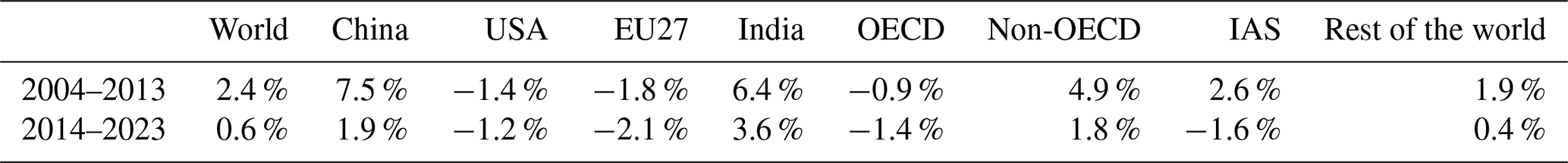
Decomposing emission changes into the components of growth, a Kaya decomposition, helps give an initial understanding of the drivers of the changes (Peters et al., 2017b). The reduction in growth in global fossil CO₂ emissions in the last decade is due to slightly weaker economic growth, accelerating declines in CO₂ emissions per unit energy, and sustained declines in energy per unit GDP (Fig. 17). These trends are a supposition of the trends at the national level. Fossil CO₂ emission declines in the USA and EU27 are primarily driven by slightly weaker economic growth since the global financial crisis (GFC) in 2008–2009, sustained declines in energy per GDP, and sustained declines in CO₂ emissions per unit energy with a slight acceleration in the USA in the last decade. In contrast, fossil CO₂ emissions continue to grow in non-OECD countries, although the growth rate has slowed from 4.9 % yr⁻¹ during the 2004–2013 decade to 1.8 % yr⁻¹ in the last decade (Table 9). Representing 47 % of non-OECD emissions in 2023, a large part of this slowdown is due to China, which has seen emissions growth decline from 7.5 % yr⁻¹ in the 2004–2013 decade to 1.9 % yr⁻¹ in the last decade. Excluding China, non-OECD emissions grew at 3 % yr⁻¹ in the 2004–2013 decade compared to 1.7 % yr⁻¹ in the last decade. China had weaker economic growth in the 2000s compared to the 2010s, and the rate of reduction in the energy intensity of economic production has weakened significantly since 2015, with accelerating declines in CO₂ emissions per unit energy (Fig. 17). India has had strong economic growth that has not been offset by declines in energy per GDP or declines in CO₂ emissions per unit energy, driving up fossil CO₂ emissions. Despite the high deployment of renewables in some countries (e.g. China, India), fossil energy sources continue to grow to meet growing energy demand (Le Quéré et al., 2019). In the rest of the world, economic growth has slowed considerably in the last decade but has only been partly offset by declines in energy or carbon intensity, leading to growing emissions.

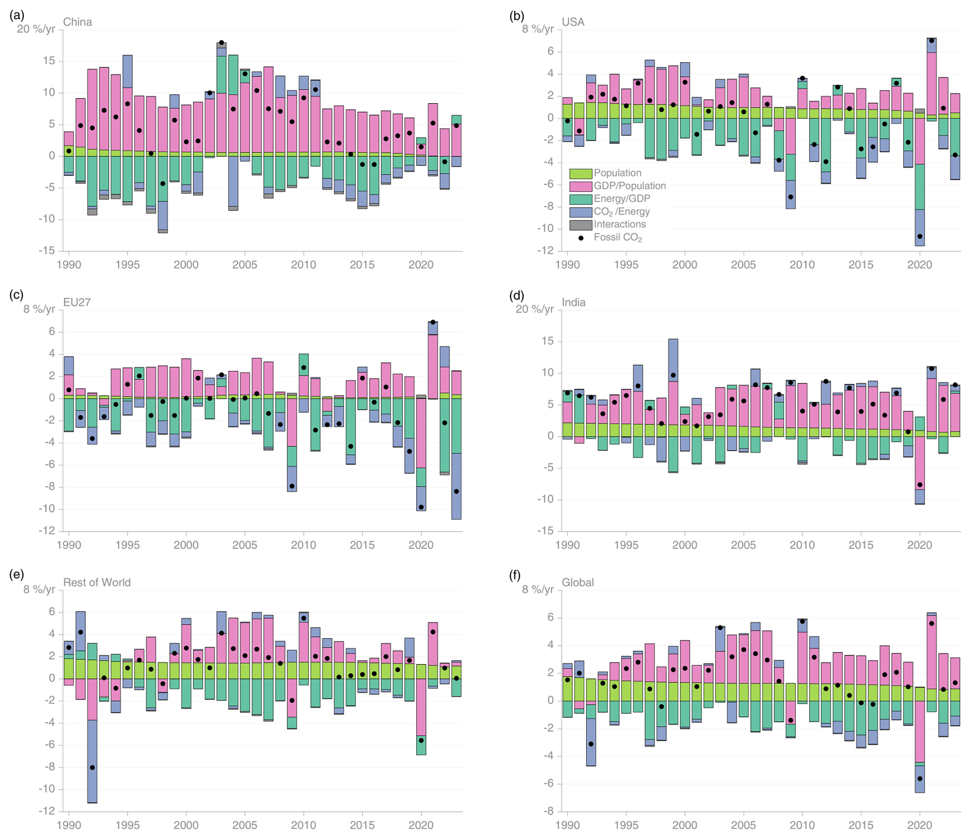
Figure 17 Kaya decomposition of the main drivers of fossil CO₂ emissions, considering population, GDP per person, energy per GDP, and CO₂ emissions per energy unit, for China (a), the USA (b), EU27 (c), India (d), the rest of the world (e), and world (f). Black dots are the annual fossil CO₂ emissions growth rate; coloured bars are the contributions from the different drivers to this growth rate. A general trend is that population and GDP growth put upward pressure on emissions (positive values), while energy per GDP and, more recently, CO₂ emissions per energy unit put downward pressure on emissions (negative values). Both the COVID-19-induced drop during 2020 and the recovery in 2021 led to a stark contrast to previous years, with different drivers in each region.

Globally, fossil CO₂ emissions growth is slowing, and this is due in part to the emergence of climate policy (Eskander and Fankhauser, 2020; Le Quéré et al., 2019) and technological change, which are leading to a shift from coal to gas and growth in renewable energies and reduced expansion of coal capacity. At the aggregated global level, decarbonization has shown a strong and growing signal in the last decade, with smaller contributions from lower economic growth and declines in energy per GDP (Fig. 17). Altogether, global fossil CO₂ emissions are still growing (average of 0.6 % yr⁻¹ over the 2014–2023 decade), and they are far from the reductions needed to meet the ambitious climate goals of the UNFCCC Paris Agreement.

Lastly, we update the remaining carbon budget (RCB) based on two studies, the IPCC AR6 (Canadell et al., 2021) and the revision of the IPCC AR6 estimates (Forster et al., 2024; Lamboll et al., 2023). We update the RCB assessed by the IPCC AR6 (Canadell et al., 2021), accounting for the 2020–2024 estimated emissions from fossil fuel combustion (E_FOS) and land-use changes (E_LUC). From January 2025, the IPCC AR6 RCB (50 % likelihood) for limiting global warming to 1.5, 1.7, and 2 °C is estimated to amount to 85, 180, and 315 GtC (305, 655, 1155 GtCO₂). The Forster et al. (2024) study proposed a significantly lower RCB than IPCC AR6, with the largest reduction being due to an update of the climate emulator (MAGICC) used to estimate the warming contribution of non-CO₂ agents and due to the warming (i.e. emissions) that occurred over the 2020–2023 period. We update the Forster et al. (2024) budget, accounting for the 2024 estimated emissions from fossil fuel combustion (E_FOS) and land-use changes (E_LUC). From January 2025, the Forster et al. (2024) RCB (50 % likelihood) for limiting global warming to 1.5, 1.7, and 2 °C is estimated to amount to 45, 140, and 290 GtC (160, 510, 1060 GtCO₂), significantly smaller than the updated IPCC AR6 estimate. Both the original IPCC AR6 and the Forster et al. (2024) estimates include the Earth system uncertainty in the climate response to cumulative CO₂ emissions, which is reflected through the percent likelihood of exceeding the given temperature threshold, an additional uncertainty of ±220 GtCO₂ due to alternative non-CO₂ emission scenarios, and other sources of uncertainties (see Canadell et al., 2021). The two sets of estimates overlap when considering all uncertainties.

Here, we take the average of our 2024 update of both the IPCC AR6 and the Forster et al. (2024) estimates, giving a remaining carbon budget (50 % likelihood) for limiting global warming to 1.5, 1.7, and 2 °C of 65, 160, and 305 GtC (235, 585, 1110 GtCO₂), respectively, starting from January 2025. We emphasize the large uncertainties, particularly when close to the global warming limit of 1.5 °C. These 1.5, 1.7, and 2 °C remaining carbon budgets correspond to about 6, 14, and 27 years, respectively, from the beginning of 2025, at the 2024 level of total anthropogenic CO₂ emissions. Reaching net-zero CO₂ emissions by 2050 entails cutting total anthropogenic CO₂ emissions by about 0.4 GtC (1.6 GtCO₂), 3.9 % of 2024 emissions, each year on average, comparable to the decrease in E_FOS observed in 2020 during the COVID-19 pandemic. However, this would lead to cumulative emissions over 2025–2050 of 145 GtC (530 GtCO₂), well above the remaining carbon budget of 65 GtC to limit global warming to 1.5 °C but still within the remaining budget of 160 GtC to limit warming to 1.7 °C (in phase with the “well below 2 °C” ambition of the Paris Agreement). Even reaching net-zero CO₂ globally by 2040, which would require annual emissions cuts of 0.7 GtC (2.5 GtCO₂) on average, would still exceed the remaining carbon budget for 1.5 °C, with 90 GtC (325 GtCO₂) of cumulative emissions over 2025–2040, unless the global emissions trajectory becomes net negative (i.e. more anthropogenic CO₂ sinks than emissions) after 2040.

5 Discussion

Each year when the global carbon budget is published, each flux component is updated for all previous years to consider corrections that are the result of further scrutiny and verification of the underlying data in the primary input datasets. Annual estimates may be updated with improvements in data quality and timeliness (e.g. to eliminate the need for extrapolation of forcing data such as land-use data). Of all terms in the global budget, only the fossil CO₂ emissions and the growth rate in atmospheric CO₂ concentration are based primarily on empirical inputs supporting annual estimates in this carbon budget. The carbon budget imbalance, still an imperfect measure, provides a strong indication of the limitations in observations, in understanding and representing processes in models, and/or in the integration of the carbon budget components.

The persistent unexplained variability in the carbon budget imbalance limits our ability to verify reported emissions (Peters et al., 2017a) and suggests we do not yet have a complete understanding of the underlying carbon cycle dynamics on annual to decadal timescales. Resolving most of this unexplained variability should be possible through different and complementary approaches. First, as intended with our annual updates, the imbalance as an error term should be reduced by improvements of individual components of the global carbon budget that follow from improving the underlying data and statistics and by improving the models through the resolution of some of the key uncertainties detailed in Table 10. Second, additional clues to the origin and processes responsible for the variability in the budget imbalance could be obtained through closer scrutiny of carbon variability in light of other Earth system data (e.g. heat balance, water balance) and the use of a wider range of biogeochemical observations to better understand the land–ocean partitioning of the carbon imbalance, such as the constraint from atmospheric oxygen included this year. Finally, additional information could also be obtained through better inclusion of process knowledge at the regional level and through the introduction of inferred fluxes such as those based on satellite XCO₂ retrievals. The limit of the resolution of the carbon budget imbalance is still unclear but most certainly has not yet been reached given the possibilities for improvements that lie ahead.

Table 10 Major known sources of uncertainties in each component of the global carbon budget, defined as input data or processes that have a demonstrated effect of at least ±0.3 GtC yr⁻¹.

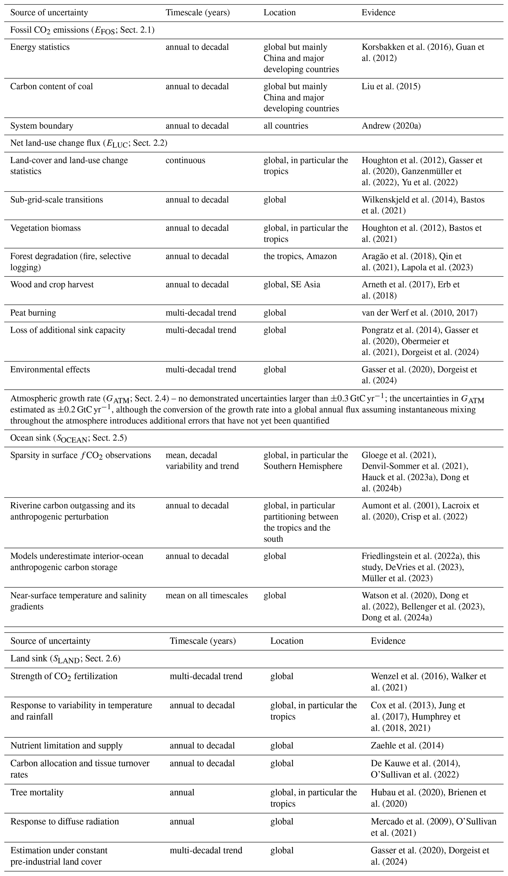
Estimates of global fossil CO₂ emissions from different datasets are in relatively good agreement when the different system boundaries of these datasets are considered (Andrew, 2020a). But while estimates of E_FOS are derived from reported activity data requiring much fewer complex transformations than some other components of the budget, uncertainties remain, and one reason for the apparently low variation between datasets is precisely the reliance on the same underlying reported energy data. The budget excludes some sources of fossil CO₂ emissions, which available evidence suggests are relatively small (< 1 %). We have added emissions from lime production in China and the USA, but these are still absent in most other non-Annex I countries and before 1990 in other Annex I countries.

Estimates of E_LUC suffer from a range of intertwined issues, including the poor quality of historical land-cover and land-use change maps, the rudimentary representation of management processes in most models, and the confusion in methodologies and boundary conditions used across methods (e.g. Arneth et al., 2017; Pongratz et al., 2014; see also the Supplement, Sect. S6.4, on the loss of sink capacity; Bastos et al., 2021). Uncertainties in current and historical carbon stocks in soils and vegetation also add uncertainty to the E_LUC estimates. Unless a major effort to resolve these issues is made, little progress is expected in the resolution of E_LUC. This is particularly concerning given the growing importance of E_LUC for climate mitigation strategies and the large issues in the quantification of the cumulative emissions over the historical period that arise from large uncertainties in E_LUC.

By adding the DGVM estimates of CO₂ fluxes due to environmental change from countries' managed forest areas (part of S_LAND in this budget) to the budget E_LUC estimate, we successfully reconciled the large gap between our E_LUC estimate and the land-use flux from NGHGIs using the approach described in Grassi et al. (2021) for future scenarios and in Grassi et al. (2023) using data from the Global Carbon Budget 2021. The updated data presented here can be used for potential adjustments in the policy context, e.g. to help assess the collective countries' progress towards the goal of the Paris Agreement and to avoid double accounting for the sink in managed forests. In the absence of this adjustment, collective progress would hence appear better than it is (Grassi et al., 2021). The application of this adjustment is also recommended in the UNFCCC Synthesis Report for the first Global Stocktake (UNFCCC, 2022) whenever a comparison between LULUCF fluxes reported by countries and the global emissions estimates of the IPCC is conducted. However, this adjustment should be seen as a short-term and pragmatic fix based on existing data rather than as a definitive solution to bridge the differences between global models and national inventories. Additional steps are needed to understand and reconcile the remaining differences, some of which are relevant at the country level (Grassi et al., 2023; Schwingshackl et al., 2022).

The comparison of GOBMs, fCO₂ products, and inversions highlights a substantial discrepancy in the temporal evolution of S_OCEAN in the Southern Ocean and northern high latitudes (Fig. 14; Hauck et al., 2023a) and in the mean S_OCEAN in the tropics. A large part of the uncertainty in the mean fluxes stems from the regional distribution of the river flux adjustment term. The current distribution simulates the largest share of the outgassing occurring in the tropics (Lacroix et al., 2020). The long-standing sparse data coverage of fCO₂ observations in the Southern Hemisphere compared to the Northern Hemisphere (e.g. Takahashi et al., 2009) continues to exist (Bakker et al., 2016, 2024; Fig. S1) and to lead to substantially higher uncertainty in the S_OCEAN estimate for the Southern Hemisphere (Watson et al., 2020; Gloege et al., 2021; Hauck et al., 2023a). This discrepancy, which also hampers model improvement, points to the need for increased high-quality fCO₂ observations especially in the Southern Ocean. At the same time, model uncertainty is illustrated by the large spread of individual GOBM estimates (indicated by shading in Fig. 14) and highlights the need for model improvement. The issue of diverging trends in S_OCEAN from different methods is smaller this year because the trend in the fCO₂ products was revised downwards with the data available in this GCB release, but it remains a matter of concern. Recent and ongoing work suggests that the fCO₂ products may overestimate the trend (Hauck et al., 2023a; see the Supplement, Sect. S3.4), though the full fCO₂-product ensemble remains to be tested. A data-constrained model approach suggests that the GOBMs underestimate the amplitude of decadal variability but that the fCO₂ products overestimate the trend (Mayot et al., 2024). At the same time, evidence is accumulating that GOBMs likely underestimate the mean flux (Sect. 3.6.2; Terhaar et al., 2022; DeVries et al., 2023; Müller et al., 2023; Dong et al., 2024a). The independent constraint from atmospheric oxygen measurements gives a larger sink for the past decade and a steeper trend. However, the estimate is consistent within uncertainties with S_OCEAN, with the relatively large ocean sink in the fCO₂ products and some of the GOBMs. The assessment of the net land–atmosphere exchange from DGVMs and atmospheric inversions also shows substantial discrepancy, particularly for the estimate of the net land flux over the northern extra-tropics. This discrepancy highlights the difficulty of quantifying complex processes (CO₂ fertilization, nitrogen deposition and fertilizers, climate change and variability, land management, etc.) that collectively determine the net land CO₂ flux. Resolving the differences in the Northern Hemisphere land sink will require the consideration and inclusion of larger quantities of observations.

We provide metrics for the evaluation of the ocean and land models and the atmospheric inversions (Figs. S2 to S4, Table S11). These metrics expand the use of observations in the global carbon budget, helping (1) to support improvements in the ocean and land carbon models that produce the sink estimates and (2) to constrain the representation of key underlying processes in the models and to allocate the regional partitioning of the CO₂ fluxes. The introduction of process-based metrics targeted to evaluate the simulation of S_OCEAN in the ocean biogeochemistry models is an important addition to the evaluation based on ocean carbon observations. This is an initial step towards the introduction of a broader range of observations and more stringent model evaluation that we hope will support continued improvements in the annual estimates of the global carbon budget.

We have previously established that a sustained decrease of −1 % in global emissions could be detected at the 66 % likelihood level after a decade only (Peters et al., 2017a). Similarly, a change in behaviour of the land and/or ocean carbon sink would take as long to detect and much longer if it emerges more slowly. To continue reducing the carbon imbalance on annual to decadal timescales, regionalizing the carbon budget and integrating multiple variables are powerful ways to shorten the detection limit and ensure the research community can rapidly identify issues of concern in the evolution of the global carbon cycle under the current rapid and unprecedented changing environmental conditions.

6 Conclusions

The estimation of global CO₂ emissions and sinks is a major effort by the carbon cycle research community that requires a careful compilation and synthesis of measurements, statistical estimates, and model results. The delivery of an annual carbon budget serves two purposes. First, there is a large demand for up-to-date information on the state of the anthropogenic perturbation of the climate system and its underpinning causes. A broad stakeholder community relies on the datasets associated with the annual carbon budget including scientists, policymakers, businesses, journalists, and non-governmental organizations engaged in adapting to and mitigating human-driven climate change. Second, over recent decades we have seen unprecedented changes in human and biophysical environments (e.g. changes in the growth of fossil fuel emissions, impact of COVID-19 pandemic, Earth's warming, and strength of the carbon sinks), which call for frequent assessments of the state of the planet, a better quantification of the causes of changes in the contemporary global carbon cycle, and an improved capacity to anticipate the evolution of the global carbon cycle in the future. Building this scientific understanding to meet the extraordinary climate mitigation challenge requires frequent, robust, transparent, and traceable datasets and methods that can be scrutinized and replicated. Via living data, this paper helps to keep track of new budget updates.

7 Data availability

The data presented here are made available in the belief that their wide dissemination will lead to greater understanding and new scientific insights of how the carbon cycle works, how humans are altering it, and how we can mitigate the resulting human-driven climate change. Full contact details and information on how to cite the data shown here are given at the top of each page in the accompanying database and are summarized in Table 2.

The accompanying database includes three Excel files organized in the following spreadsheets.

The file Global_Carbon_Budget_2024v1.0.xlsx includes the following:

1. a summary,

2. the global carbon budget (1959–2023),

3. the historical global carbon budget (1750–2023),

4. global CO₂ emissions from fossil fuels and cement production by fuel type and the per capita emissions (1850–2023),

5. CO₂ emissions from land-use change from the individual bookkeeping models (1959–2023),

6. the ocean CO₂ sink from the individual global ocean biogeochemistry models and fCO₂ products (1959–2023),

7. the terrestrial CO₂ sink from the individual DGVMs (1959–2023),

8. the cement carbonation CO₂ sink (1959–2023).

The file National_Fossil_Carbon_Emissions_2024v1.0.xlsx includes the following:

1. summary,

2. territorial country CO₂ emissions from fossil fuels and cement production (1850–2023),

3. consumption country CO₂ emissions from fossil fuels and cement production and emissions transfer from the international trade of goods and services (1990–2020) using CDIAC/UNFCCC data as reference,

4. emissions transfers (consumption minus territorial emissions, 1990–2020),

5. country definitions.

The file National_LandUseChange_Carbon_Emissions_2024v1.0.xlsx includes the following:

1. a summary,

2. territorial country CO₂ emissions from land-use change (1850–2023) from three bookkeeping models.

All three spreadsheets are published by the Integrated Carbon Observation System (ICOS) Carbon Portal and are available at https://doi.org/10.18160/GCP-2024 (Friedlingstein et al., 2024). National emissions data are also available at https://doi.org/10.5281/zenodo.13981696 (Andrew and Peters, 2024), from the Global Carbon Atlas (http://www.globalcarbonatlas.org/, Global Carbon Project, 2024) and from Our World in Data (2024, https://ourworldindata.org/co2-emissions).