the Creative Commons Attribution 4.0 License.
the Creative Commons Attribution 4.0 License.
 | 11 Nov 2022
Global Carbon Budget 2022
Pierre Friedlingstein
Michael O'Sullivan
Matthew W. Jones
Robbie M. Andrew
Luke Gregor
Judith Hauck
Corinne Le Quéré
Ingrid T. Luijkx
Are Olsen
Glen P. Peters
Wouter Peters
Julia Pongratz
Clemens Schwingshackl
Stephen Sitch
Josep G. Canadell
Philippe Ciais
Robert B. Jackson
Simone R. Alin
Ramdane Alkama
Almut Arneth
Vivek K. Arora
Nicholas R. Bates
Meike Becker
Nicolas Bellouin
Henry C. Bittig
Laurent Bopp
Frédéric Chevallier
Louise P. Chini
Margot Cronin
Wiley Evans
Stefanie Falk
Richard A. Feely
Thomas Gasser
Marion Gehlen
Thanos Gkritzalis
Lucas Gloege
Giacomo Grassi
Nicolas Gruber
Özgür Gürses
Ian Harris
Matthew Hefner
Richard A. Houghton
George C. Hurtt
Yosuke Iida
Tatiana Ilyina
Atul K. Jain
Annika Jersild
Koji Kadono
Etsushi Kato
Daniel Kennedy
Kees Klein Goldewijk
Jürgen Knauer
Jan Ivar Korsbakken
Peter Landschützer
Nathalie Lefèvre
Keith Lindsay
Junjie Liu
Gregg Marland
Nicolas Mayot
Matthew J. McGrath
Nicolas Metzl
Natalie M. Monacci
David R. Munro
Shin-Ichiro Nakaoka
Yosuke Niwa
Kevin O'Brien
Tsuneo Ono
Paul I. Palmer
Naiqing Pan
Denis Pierrot
Katie Pocock
Benjamin Poulter
Laure Resplandy
Eddy Robertson
Christian Rödenbeck
Carmen Rodriguez
Thais M. Rosan
Jörg Schwinger
Roland Séférian
Jamie D. Shutler
Ingunn Skjelvan
Tobias Steinhoff
Adrienne J. Sutton
Colm Sweeney
Shintaro Takao
Toste Tanhua
Pieter P. Tans
Xiangjun Tian
Hanqin Tian
Bronte Tilbrook
Hiroyuki Tsujino
Francesco Tubiello
Guido R. van der Werf
Anthony P. Walker
Rik Wanninkhof
Chris Whitehead
Anna Willstrand Wranne
Rebecca Wright
Wenping Yuan
Sönke Zaehle
Jiye Zeng
Land CO2 sinkand ending with the section
Processes not included in the global carbon budget. We corrected the article accordingly. Nothing else has changed.
Accurate assessment of anthropogenic carbon dioxide (CO2) emissions and their redistribution among the atmosphere, ocean, and terrestrial biosphere in a changing climate is critical to better understand the global carbon cycle, support the development of climate policies, and project future climate change. Here we describe and synthesize data sets and methodologies to quantify the five major components of the global carbon budget and their uncertainties. Fossil CO2 emissions (EFOS) are based on energy statistics and cement production data, while emissions from land-use change (ELUC), mainly deforestation, are based on land use and land-use change data and bookkeeping models. Atmospheric CO2 concentration is measured directly, and its growth rate (GATM) is computed from the annual changes in concentration. The ocean CO2 sink (SOCEAN) is estimated with global ocean biogeochemistry models and observation-based data products. The terrestrial CO2 sink (SLAND) is estimated with dynamic global vegetation models. The resulting carbon budget imbalance (BIM), the difference between the estimated total emissions and the estimated changes in the atmosphere, ocean, and terrestrial biosphere, is a measure of imperfect data and understanding of the contemporary carbon cycle. All uncertainties are reported as ±1σ.
For the year 2021, EFOS increased by 5.1 % relative to 2020, with fossil emissions at 10.1 ± 0.5 GtC yr−1 (9.9 ± 0.5 GtC yr−1 when the cement carbonation sink is included), and ELUC was 1.1 ± 0.7 GtC yr−1, for a total anthropogenic CO2 emission (including the cement carbonation sink) of 10.9 ± 0.8 GtC yr−1 (40.0 ± 2.9 GtCO2). Also, for 2021, GATM was 5.2 ± 0.2 GtC yr−1 (2.5 ± 0.1 ppm yr−1), SOCEAN was 2.9 ± 0.4 GtC yr−1, and SLAND was 3.5 ± 0.9 GtC yr−1, with a BIM of −0.6 GtC yr−1 (i.e. the total estimated sources were too low or sinks were too high). The global atmospheric CO2 concentration averaged over 2021 reached 414.71 ± 0.1 ppm. Preliminary data for 2022 suggest an increase in EFOS relative to 2021 of +1.0 % (0.1 % to 1.9 %) globally and atmospheric CO2 concentration reaching 417.2 ppm, more than 50 % above pre-industrial levels (around 278 ppm). Overall, the mean and trend in the components of the global carbon budget are consistently estimated over the period 1959–2021, but discrepancies of up to 1 GtC yr−1 persist for the representation of annual to semi-decadal variability in CO2 fluxes. Comparison of estimates from multiple approaches and observations shows (1) a persistent large uncertainty in the estimate of land-use change emissions, (2) a low agreement between the different methods on the magnitude of the land CO2 flux in the northern extratropics, and (3) a discrepancy between the different methods on the strength of the ocean sink over the last decade. This living data update documents changes in the methods and data sets used in this new global carbon budget and the progress in understanding of the global carbon cycle compared with previous publications of this data set. The data presented in this work are available at https://doi.org/10.18160/GCP-2022 (Friedlingstein et al., 2022b).
-
Please read the editorial note first before accessing the article.
-
Article
(15731 KB)
-
Please read the editorial note first before accessing the article.


Global fossil CO2 emissions (including cement carbonation) further increased in 2022, being now slightly above their pre-COVID-19 pandemic 2019 level. The 2021 emission increase was 0.46 GtC yr−1 (1.7 GtCO2 yr−1), bringing 2021 emissions to 9.9 ± 0.5 GtC yr−1 (36.3 ± 1.8 GtCO2 yr−1), same as the 2019 emissions level. Preliminary estimates based on data available suggest fossil CO2 emissions continued to increase by 1.0 % in 2022 relative to 2021 (0.1 % to 1.9 %), bringing emissions of 10.0 GtC yr−1 (36.6 GtCO2 yr−1), slightly above the 2019 level.
Emissions from coal, oil, and gas in 2022 are expected to be above their 2021 levels (by 1.0 %, 2.2 % and −0.2 % respectively). Regionally, emissions in 2022 are expected to have decreased by 0.9 % in China (3.1 GtC, 11.4 GtCO2) and 0.8 % in the European Union (0.8 GtC, 2.8 GtCO2) but increased by 1.5 % in the United States (1.4 GtC, 5.1 GtCO2), 6 % in India (0.8 GtC, 2.9 GtCO2), and 1.7 % in the rest of the world (4.2 GtC, 15.4 GtCO2).
Fossil CO2 emissions decreased in 24 countries during the decade 2012–2021. Altogether, these 24 countries contributed about 2.4 GtC yr−1 (8.8 GtCO2) fossil fuel CO2 emissions over the last decade, about a quarter of global CO2 fossil emissions.
Global CO2 emissions from land use, land-use change, and forestry (LUC) averaged at 1.2 ± 0.7 GtC yr−1 (4.5 ± 2.6 GtCO2 yr−1) for the 2012–2021 period with a preliminary projection for 2022 of 1.1 ± 0.7 GtC yr−1 (3.9 ± 2.6 GtCO2 yr−1). A small decrease over the past 2 decades is not robust given the large model uncertainty. Emissions from deforestation, the main driver of global gross sources, remain high at 1.8 ± 0.4 GtC yr−1 over the 2012–2021 period, highlighting the strong potential for emissions reductions when halting deforestation. Sequestration of 0.9 ± 0.3 GtC yr−1 through afforestation or reafforestation and forestry offsets half of the deforestation emissions. Emissions from other land-use transitions and from peat drainage and peat fire add further small contributions. The highest emitters during 2012–2021 in descending order were Brazil, Indonesia, and the Democratic Republic of the Congo, with these three countries contributing more than half of the global total land-use emissions.
The remaining carbon budget for a 50 % likelihood to limit global warming to 1.5, 1.7, and 2 ∘C has, respectively, reduced to 105 GtC (380 GtCO2), 200 GtC (730 GtCO2), and 335 GtC (1230 GtCO2) from the beginning of 2023, equivalent to 9, 18, and 30 years, assuming 2022 emissions levels. Total anthropogenic emissions were 11.0 GtC yr−1 (40.2 GtCO2 yr−1) in 2021, with a preliminary estimate of 11.1 GtC yr−1 (40.5 GtCO2 yr−1) for 2022. The remaining carbon budget to keep global temperatures below these climate targets has shrunk by 32 GtC (121 GtCO2) since the IPCC AR6 Working Group 1 assessment based on data up to 2019. Reaching zero CO2 emissions by 2050 entails a total anthropogenic CO2 emissions linear decrease by about 0.4 GtC (1.4 GtCO2) each year, comparable to the decrease during 2020, highlighting the scale of the action needed.
The concentration of CO2 in the atmosphere is set to reach 417.2 ppm in 2022, 51 % above pre-industrial levels. The atmospheric CO2 growth was 5.2 ± 0.02 GtC yr−1 during the decade 2012–2021 (48 % of total CO2 emissions) with a preliminary 2022 growth rate estimate of around 5.3 GtC yr−1 (2.5 ppm).
The ocean CO2 sink resumed a more rapid growth in the past 2 decades after low or no growth during the 1991–2002 period. However, the growth of the ocean CO2 sink in the past decade has an uncertainty of a factor of 3, with estimates based on data products and estimates based on models showing an ocean sink trend of +0.7 GtC yr−1 per decade and +0.2 GtC yr−1 per decade since 2010, respectively. The discrepancy in the trend originates from all latitudes but is largest in the Southern Ocean. The ocean CO2 sink was 2.9 ± 0.4 GtC yr−1 during the decade 2012–2021 (26 % of total CO2 emissions), with a similar preliminary estimate of 2.9 GtC yr−1 for 2022.
The land CO2 sink continued to increase during the 2012–2021 period primarily in response to increased atmospheric CO2, albeit with large interannual variability. The land CO2 sink was 3.1 ± 0.6 GtC yr−1 during the decade 2012–2021 (29 % of total CO2 emissions), 0.4 GtC yr−1 larger than during the previous decade (2000–2009), with a preliminary 2022 estimate of around 3.4 GtC yr−1. Year-to-year variability in the land sink is about 1 GtC yr−1 and dominates the year-to-year changes in the global atmospheric CO2 concentration, implying that small annual changes in anthropogenic emissions (such as the fossil fuel emission decrease in 2020) are hard to detect in the atmospheric CO2 observations.
The concentration of carbon dioxide (CO2) in the atmosphere has increased from approximately 278 parts per million (ppm) in 1750 (Gulev et al., 2021), the beginning of the Industrial Era, to 414.7 ± 0.1 ppm in 2021 (Dlugokencky and Tans, 2022; Fig. 1). The atmospheric CO2 increase above pre-industrial levels was, initially, primarily caused by the release of carbon to the atmosphere from deforestation and other land-use change activities (Canadell et al., 2021). While emissions from fossil fuels started before the Industrial Era, they became the dominant source of anthropogenic emissions to the atmosphere from around 1950, and their relative share has continued to increase until present. Anthropogenic emissions occur on top of an active natural carbon cycle that circulates carbon between the reservoirs of the atmosphere, ocean, and terrestrial biosphere on timescales from sub-daily to millennia, while exchanges with geologic reservoirs occur at longer timescales (Archer et al., 2009).
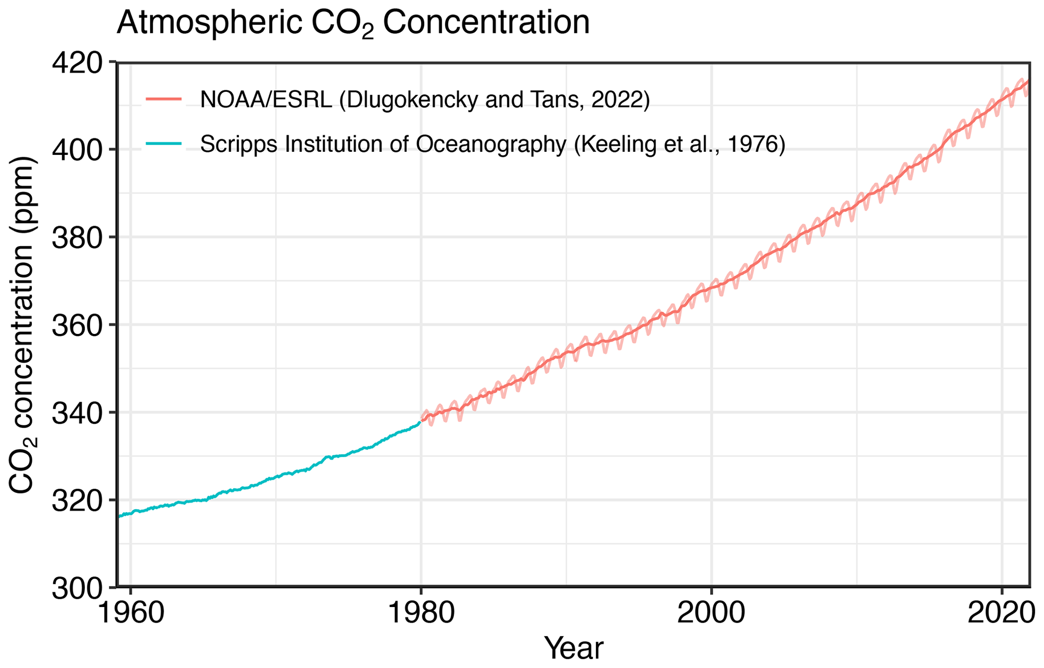
Figure 1Surface average atmospheric CO2 concentration (ppm). Since 1980, monthly data are from NOAA/GML (Dlugokencky and Tans, 2022) and are based on an average of direct atmospheric CO2 measurements from multiple stations in the marine boundary layer (Masarie and Tans, 1995). The 1958–1979 monthly data are from the Scripps Institution of Oceanography, based on an average of direct atmospheric CO2 measurements from the Mauna Loa and South Pole stations (Keeling et al., 1976). To account for the difference in mean CO2 and seasonality between the NOAA/GML and the Scripps station networks used here, the Scripps surface average (from two stations) was de-seasonalized and adjusted to match the NOAA/GML surface average (from multiple stations) by adding the mean difference of 0.667 ppm, calculated here from overlapping data during 1980–2012.
The global carbon budget (GCB) presented here refers to the mean, variations, and trends in the perturbation of CO2 in the environment, referenced to the beginning of the Industrial Era (defined here as 1750). This paper describes the components of the global carbon cycle over the historical period with a stronger focus on the recent period (since 1958, the onset of atmospheric CO2 measurements), the last decade (2012–2021), the last year (2021), and the current year (2022). Finally, it provides cumulative emissions from fossil fuels and land-use change since the year 1750 (the pre-industrial period) and since the year 1850 (the reference year for historical simulations in IPCC AR6) (Eyring et al., 2016).
We quantify the input of CO2 to the atmosphere by emissions from human activities; the growth rate of atmospheric CO2 concentration; and the resulting changes in the storage of carbon in the land and ocean reservoirs in response to increasing atmospheric CO2 levels, climate change and variability, and other anthropogenic and natural changes (Fig. 2). An understanding of this perturbation budget over time and the underlying variability and trends of the natural carbon cycle is necessary to understand the response of natural sinks to changes in climate, CO2, and land-use change drivers and to quantify emissions compatible with a given climate stabilization target.
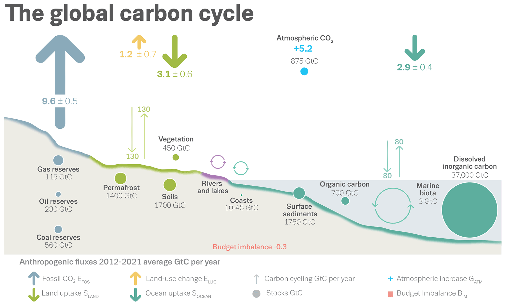
Figure 2Schematic representation of the overall perturbation of the global carbon cycle caused by anthropogenic activities averaged globally for the decade 2012–2021. See legends for the corresponding arrows and units. The uncertainty in the atmospheric CO2 growth rate is very small (±0.02 GtC yr−1) and is neglected for the figure. The anthropogenic perturbation occurs on top of an active carbon cycle, with fluxes and stocks represented in the background and taken from Canadell et al. (2021) for all numbers, except for the carbon stocks in coasts, which are from a literature review of coastal marine sediments (Price and Warren, 2016).
The components of the CO2 budget that are reported annually in this paper include separate and independent estimates for the CO2 emissions from (1) fossil fuel combustion and oxidation from all energy and industrial processes, including cement production and carbonation (EFOS; GtC yr−1), and (2) the emissions resulting from deliberate human activities on land, including those leading to land-use change (ELUC; GtC yr−1) and their partitioning among (3) the growth rate of atmospheric CO2 concentration (GATM; GtC yr−1) and the uptake of CO2 (the “CO2 sinks”) in (4) the ocean (SOCEAN; GtC yr−1) and (5) on land (SLAND; GtC yr−1). The CO2 sinks as defined here conceptually include the response of the land (including inland waters and estuaries) and ocean (including coastal and marginal seas) to elevated CO2 and changes in climate and other environmental conditions, although in practice not all processes are fully accounted for (see Sect. 2.7). Global emissions and their partitioning among the atmosphere, ocean, and land are in balance in the real world. Due to the combination of imperfect spatial and/or temporal data coverage, errors in each estimate, and smaller terms not included in our budget estimate (discussed in Sect. 2.7), the independent estimates (1) to (5) above do not necessarily add up to zero. We therefore (i) additionally assess a set of global atmospheric inversion system results that by design close the global carbon balance (see Sect. 2.6) and (i) estimate a budget imbalance (BIM), which is a measure of the mismatch between the estimated emissions and the estimated changes in the atmosphere, land, and ocean, as follows:
GATM is usually reported in ppm yr−1, which we convert to units of carbon mass per year, GtC yr−1, using 1 ppm = 2.124 GtC (Ballantyne et al., 2012; Table 1). All quantities are presented in units of gigatonnes of carbon (GtC, 1015 gC), which is the same as petagrams of carbon (PgC; Table 1). Units of gigatonnes of CO2 (or billion tonnes of CO2) used in policy are equal to 3.664 multiplied by the value in units of GtC.
Table 1Factors used to convert carbon in various units (by convention, Unit 1 = Unit 2 × conversion).
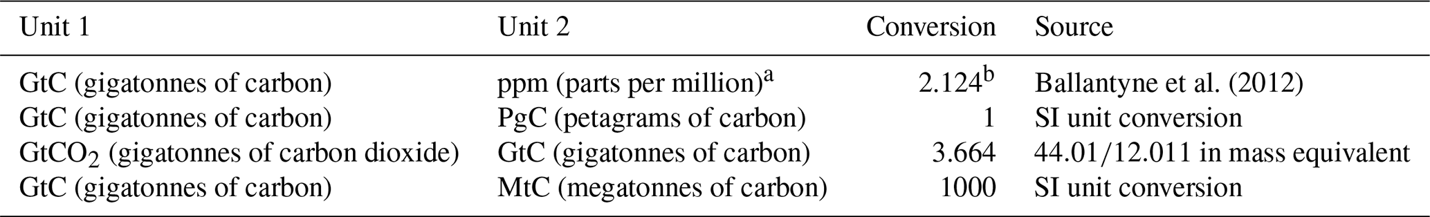
a Measurements of atmospheric CO2 concentration have units of dry-air mole fraction. “ppm” is an abbreviation for µmol mol−1 dry air. bThe use of a factor of 2.124 assumes that all of the atmosphere is well mixed within 1 year. In reality, only the troposphere is well mixed, and the growth rate of CO2 concentration in the less well-mixed stratosphere is not measured by sites from the NOAA network. Using a factor of 2.124 makes the approximation that the growth rate of CO2 concentration in the stratosphere equals that of the troposphere on a yearly basis.
We also quantify EFOS and ELUC by country, including both territorial and consumption-based accounting for EFOS (see Sect. 2), and discuss missing terms from sources other than the combustion of fossil fuels (see Sect. 2.7 and Appendix D1 and D2).
The global CO2 budget has been assessed by the Intergovernmental Panel on Climate Change (IPCC) in all assessment reports (Prentice et al., 2001; Schimel et al., 1995; Watson et al., 1990; Denman et al., 2007; Ciais et al., 2013; Canadell et al., 2021) and by others (e.g. Ballantyne et al., 2012). The Global Carbon Project (GCP, https://www.globalcarbonproject.org, last access: 25 September 2022) has coordinated this cooperative community effort for the annual publication of global carbon budgets for the year 2005 (Raupach et al., 2007; including fossil emissions only), year 2006 (Canadell et al., 2007), year 2007 (GCP, 2007), year 2008 (Le Quéré et al., 2009), year 2009 (Friedlingstein et al., 2010), year 2010 (Peters et al., 2012b), year 2012 (Le Quéré et al., 2013; Peters et al., 2013), year 2013 (Le Quéré et al., 2014), year 2014 (Le Quéré et al., 2015a; Friedlingstein et al., 2014), year 2015 (Jackson et al., 2016; Le Quéré et al., 2015b), year 2016 (Le Quéré et al., 2016), year 2017 (Le Quéré et al., 2018a; Peters et al., 2017), year 2018 (Le Quéré et al., 2018b; Jackson et al., 2018), year 2019 (Friedlingstein et al., 2019; Jackson et al., 2019; Peters et al., 2020), year 2020 (Friedlingstein et al., 2020; Le Quéré et al., 2021), and more recently the year 2021 (Friedlingstein et al., 2022a; Jackson et al., 2022). Each of these papers updated previous estimates with the latest available information for the entire time series.
We adopt a range of ±1 standard deviation (σ) to report the uncertainties in our estimates, representing a likelihood of 68 % that the true value will be within the provided range if the errors have a Gaussian distribution and no bias is assumed. This choice reflects the difficulty of characterizing the uncertainty in the CO2 fluxes between the atmosphere and the ocean and land reservoirs individually, particularly on an annual basis, as well as the difficulty of updating the CO2 emissions from land-use change. A likelihood of 68 % provides an indication of our current capability to quantify each term and its uncertainty given the available information. The uncertainties reported here combine statistical analysis of the underlying data, assessments of uncertainties in the generation of the data sets, and expert judgement of the likelihood of results lying outside this range. The limitations of current information are discussed in the paper and have been examined in detail elsewhere (Ballantyne et al., 2015; Zscheischler et al., 2017). We also use a qualitative assessment of confidence level to characterize the annual estimates from each term based on the type, amount, quality, and consistency of the evidence as defined by the IPCC (Stocker et al., 2013).
This paper provides a detailed description of the data sets and methodology used to compute the global carbon budget estimates for the industrial period (from 1750 to 2022) and in more detail for the period since 1959. This paper is updated every year using the format of “living data” to keep a record of budget versions and the changes in new data, revisions of data, and changes in methodology that lead to changes in estimates of the carbon budget. Additional materials associated with the release of each new version will be posted at the Global Carbon Project (GCP) website (http://www.globalcarbonproject.org/carbonbudget, last access: 25 September 2022), with fossil fuel emissions also available through the Global Carbon Atlas (http://www.globalcarbonatlas.org, last access: 25 September 2022). All underlying data used to produce the budget can also be found at https://globalcarbonbudget.org/ (last access: 25 September 2022). With this approach, we aim to provide the highest transparency and traceability in the reporting of CO2, the key driver of climate change.
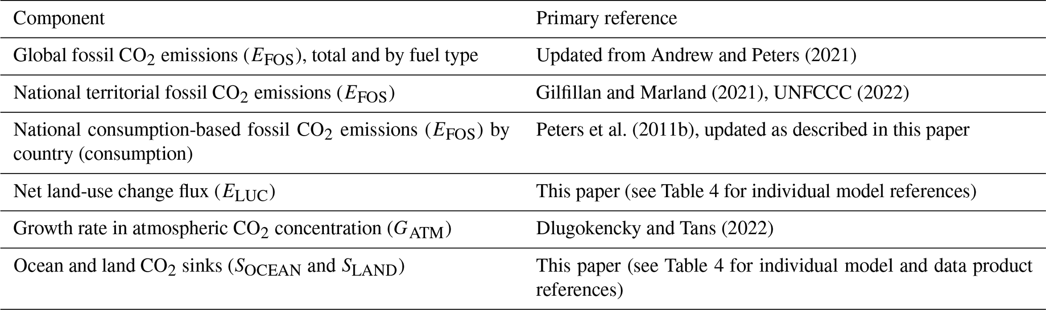
Multiple organizations and research groups around the world generated the original measurements and data used to complete the global carbon budget. The effort presented here is thus mainly one of synthesis, where results from individual groups are collated, analysed, and evaluated for consistency. We facilitate access to original data with the understanding that primary data sets will be referenced in future work (see Table 2 for how to cite the data sets). Descriptions of the measurements, models, and methodologies follow below, and detailed descriptions of each component are provided elsewhere.
Table 2How to cite the individual components of the global carbon budget presented here.
This is the 17th version of the global carbon budget and the 11th revised version in the format of a living data update in Earth System Science Data. It builds on the latest published global carbon budget of Friedlingstein et al. (2022a). The main changes are the inclusion of (1) data to year 2021 and a projection for the global carbon budget for the year 2022, (2) the inclusion of country-level estimates of ELUC, and(3) a process-based decomposition of ELUC into its main components (deforestation; afforestation, reafforestation, and wood harvest; emissions from organic soils; and net flux from other transitions).
The main methodological differences between recent annual carbon budgets (2018–2022) are summarized in Table 3, and previous changes since 2006 are provided in Table A7.
Table 3The main methodological changes in the global carbon budget since 2018. Methodological changes introduced in any given year are kept for the following years unless otherwise noted. Empty cells mean there were no methodological changes introduced that year. Table A7 lists methodological changes from the first global carbon budget publication up to 2017.
2.1 Fossil CO2 emissions (EFOS)
2.1.1 Historical period 1850–2021
The estimates of global and national fossil CO2 emissions (EFOS) include the oxidation of fossil fuels through both combustion (e.g. transport, heating) and chemical oxidation (e.g. carbon anode decomposition in aluminium refining) activities, and the decomposition of carbonates in industrial processes (e.g. the production of cement). We also include CO2 uptake from the cement carbonation process. Several emission sources are not estimated or not fully covered: coverage of emissions from lime production is not global, and decomposition of carbonates in glass and ceramic production are included only for the “Annex 1” countries of the United Nations Framework Convention on Climate Change (UNFCCC) for lack of activity data. These omissions are considered to be minor. Short-cycle carbon emissions – for example from combustion of biomass – are not included here but are accounted for in the CO2 emissions from land use (see Sect. 2.2).
Our estimates of fossil CO2 emissions are derived using the standard approach of activity data and emission factors, relying on data collection by many other parties. Our goal is to produce the best estimate of this flux, and we therefore use a prioritization framework to combine data from different sources that have used different methods, while being careful to avoid double counting and undercounting of emissions sources. The CDIAC-FF emissions data set, derived largely from UN energy data, forms the foundation, and we extend emissions to year Y-1 using energy growth rates reported by the BP energy company. We then proceed to replace estimates using data from what we consider to be superior sources, for example Annex 1 countries' official submissions to the UNFCCC. All data points are potentially subject to revision, not just the latest year. For the full details, see Andrew and Peters (2021).
Other estimates of global fossil CO2 emissions exist, and these are compared by Andrew (2020a). The most common reason for differences in estimates of global fossil CO2 emissions is a difference in which emissions sources are included in the data sets. Data sets such as those published by the energy company BP, the US Energy Information Administration, and the International Energy Agency's “CO2 emissions from fuel combustion” are all generally limited to emissions from combustion of fossil fuels. In contrast, data sets such as PRIMAP-hist, CEDS, EDGAR, and GCP's data set aim to include all sources of fossil CO2 emissions. See Andrew (2020a) for detailed comparisons and discussion.
Cement absorbs CO2 from the atmosphere over its lifetime, a process known as “cement carbonation”. We estimate this CO2 sink from 1931 onwards as the average of two studies in the literature (Cao et al., 2020; Guo et al., 2021). Both studies use the same model, developed by Xi et al. (2016), with different parameterizations and input data, with the estimate of Guo and colleagues being a revision of Xi et al. (2016). The trends of the two studies are very similar. Since carbonation is a function of both current and previous cement production, we extend these estimates to 2022 by using the growth rate derived from the smoothed cement emissions (10-year smoothing) fitted to the carbonation data. In the present budget, we always include the cement carbonation carbon sink in the fossil CO2 emission component (EFOS).
We use the Kaya Identity for a simple decomposition of CO2 emissions into the key drivers (Raupach et al., 2007). While there are variations (Peters et al., 2017), we focus here on a decomposition of CO2 emissions into population, GDP per person, energy use per GDP, and CO2 emissions per energy. Multiplying these individual components together returns the CO2 emissions. Using the decomposition, it is possible to attribute the change in CO2 emissions to the change in each of the drivers. This method gives a first-order understanding of what causes CO2 emissions to change each year.
2.1.2 The 2022 projection
We provide a projection of global CO2 emissions in 2022 by combining separate projections for China, USA, EU, India, and for all other countries combined. The methods are different for each of these. For China we combine monthly fossil fuel production data from the National Bureau of Statistics, import and export data from the Customs Administration, and monthly coal consumption estimates from SX Coal (2022), giving us partial data for the growth rates to date of natural gas, petroleum, and cement, and of the consumption itself for raw coal. We then use a regression model to project full-year emissions based on historical observations. For the USA our projection is taken directly from the Energy Information Administration's (EIA) Short-Term Energy Outlook (EIA, 2022), combined with the year-to-date growth rate of cement clinker production. For the EU we use monthly energy data from Eurostat to derive estimates of monthly CO2 emissions through July, with coal emissions extended through August using a statistical relationship with reported electricity generation from coal and other factors. Given the very high uncertainty in European energy markets in 2022, we forego our usual history-based projection techniques and instead use the year-to-date growth rate as the full-year growth rate for both coal and natural gas. EU emissions from oil are derived using the EIA's projection of oil consumption for Europe. EU cement emissions are based on available year-to-date data from three of the largest producers, Germany, Poland, and Spain. India's projected emissions are derived from estimates through July (August for oil) using the methods of Andrew (2020b) and extrapolated assuming normal seasonal patterns. Emissions for the rest of the world are derived using projected growth in economic production from the IMF (2022) combined with extrapolated changes in emissions intensity of economic production. More details on the EFOS methodology and its 2022 projection can be found in Appendix C1.
2.2 CO2 emissions from land use, land-use change, and forestry (ELUC)
2.2.1 Historical period 1850–2021
The net CO2 flux from land use, land-use change, and forestry (ELUC, called land-use change emissions in the rest of the text) includes CO2 fluxes from deforestation, afforestation, logging and forest degradation (including harvest activity), shifting cultivation (cycle of cutting forest for agriculture, then abandoning), and regrowth of forests (following wood harvest or agriculture abandonment). Emissions from peat burning and drainage are added from external data sets, with peat drainage being averaged from three spatially explicit independent data sets (see Appendix C2.1).
Three bookkeeping approaches, updated estimates each of BLUE (Hansis et al., 2015), OSCAR (Gasser et al., 2020), and H&N2017 (Houghton and Nassikas, 2017), were used to quantify gross sources and sinks and the resulting net ELUC. Uncertainty estimates were derived from the dynamic global vegetation models (DGVMs) ensemble for the time period prior to 1960, using for the recent decades an uncertainty range of ±0.7 GtC yr−1, which is a semi-quantitative measure for annual and decadal emissions and reflects our best value judgement that there is at least 68 % chance (±1σ) that the true land-use change emission lies within the given range for the range of processes considered here. This uncertainty range had been increased from 0.5 GtC yr−1 after new bookkeeping models were included that indicated a larger spread than assumed before (Le Quéré et al., 2018a). Projections for 2021 are based on fire activity from tropical deforestation and degradation and emissions from peat fires and drainage.
Our ELUC estimates follow the definition of global carbon cycle models of CO2 fluxes related to land-use and land management and differ from IPCC definitions adopted in national greenhouse gas (GHG) inventories (NGHGI) for reporting under the UNFCCC, which additionally generally include, through adoption of the IPCC so-called managed land proxy approach, the terrestrial fluxes occurring on land defined by countries as managed. This partly includes fluxes due to environmental change (e.g. atmospheric CO2 increase), which are part of SLAND in our definition. This causes the global emission estimates to be smaller for NGHGI than for the global carbon budget definition (Grassi et al., 2018). The same is the case for the Food Agriculture Organization (FAO) estimates of carbon fluxes on forest land, which include both anthropogenic and natural sources on managed land (Tubiello et al., 2021). We map the two definitions to each other, to provide a comparison of the anthropogenic carbon budget to the official country reporting to the climate convention.
2.2.2 The 2022 projection
We project the 2022 land-use emissions for BLUE, the updated H&N2017, and OSCAR, starting from their estimates for 2021 assuming unaltered peat drainage, which has low interannual variability but adjusting the highly variable emissions from peat fires, tropical deforestation, and degradation as estimated using active fire data (MCD14ML; Giglio et al., 2016). More details on the ELUC methodology can be found in Appendix C2.
2.3 Growth rate in atmospheric CO2 concentration (GATM)
2.3.1 Historical period 1850–2021
The rate of growth of the atmospheric CO2 concentration is provided for years 1959–2021 by the US National Oceanic and Atmospheric Administration Global Monitoring Laboratory (NOAA/GML; Dlugokencky and Tans, 2022), which is updated from Ballantyne et al. (2012) and includes recent revisions to the calibration scale of atmospheric CO2 measurements (Hall et al., 2021). For the 1959–1979 period, the global growth rate is based on measurements of atmospheric CO2 concentration averaged from the Mauna Loa and South Pole stations, as observed by the CO2 Program at Scripps Institution of Oceanography (Keeling et al., 1976). For the 1980–2020 time period, the global growth rate is based on the average of multiple stations selected from the marine boundary layer sites with well-mixed background air (Ballantyne et al., 2012), after fitting a smooth curve through the data for each station as a function of time and averaging by latitude band (Masarie and Tans, 1995). The annual growth rate is estimated by Dlugokencky and Tans (2022) from atmospheric CO2 concentration by taking the average of the most recent December–January months corrected for the average seasonal cycle and subtracting this same average one year earlier. The growth rate (in units of ppm yr−1) is converted to units of GtC yr−1 by multiplying by a factor of 2.124 GtC ppm−1, assuming instantaneous mixing of CO2 throughout the atmosphere (Ballantyne et al., 2012; Table 1).
Since 2020, NOAA/GML provides estimates of atmospheric CO2 concentrations with respect to a new calibration scale, referred to as WMO-CO2-X2019, in line with the recommendation of the World Meteorological Organization (WMO) Global Atmosphere Watch (GAW) community (Hall et al., 2021). The “X” in the scale name indicates that it is a mole fraction scale, how many micro-moles of CO2 in a single mole of (dry) air. The word “concentration” only loosely reflects this. The WMO-CO2-X2019 scale improves upon the earlier WMO-CO2-X2007 scale by including a broader set of standards, which contain CO2 in a wider range of concentrations that span the range 250–800 ppm (vs. 250–520 ppm for WMO-CO2-X2007). In addition, NOAA/GML made two minor corrections to the analytical procedure used to quantify CO2 concentrations, fixing an error in the second virial coefficient of CO2 and accounting for loss of a small amount of CO2 to materials in the manometer during the measurement process. The difference in concentrations measured using WMO-CO2-X2019 vs. WMO-CO2-X2007 is ∼ +0.18 ppm at 400 ppm and the observational record of atmospheric CO2 concentrations have been revised accordingly. The revisions have been applied retrospectively in all cases where the calibrations were performed by NOAA/GML, thus affecting measurements made by members of the WMO-GAW programme and other regionally coordinated programmes (e.g. Integrated Carbon Observing System, ICOS). Changes to the CO2 concentrations measured across these networks propagate to the global mean CO2 concentrations. The recalibrated data were first used to estimate GATM in the 2021 edition of the global carbon budget (Friedlingstein et al., 2022a). Friedlingstein et al. (2022a) verified that the change of scales from WMO-CO2-X2007 to WMO-CO2-X2019 made a negligible difference to the value of GATM (−0.06 GtC yr−1 during 2010–2019 and −0.01 GtC yr−1 during 1959–2019, well within the uncertainty range reported below).
The uncertainty around the atmospheric growth rate is due to four main factors. First, the long-term reproducibility of reference gas standards (around 0.03 ppm for 1σ from the 1980s; Dlugokencky and Tans, 2022). Second, small unexplained systematic analytical errors that may have a duration of several months to 2 years come and go. They have been simulated by randomizing both the duration and the magnitude (determined from the existing evidence) in a Monte Carlo procedure. Third, the network composition of the marine boundary layer with some sites coming or going, gaps in the time series at each site, and so on (Dlugokencky and Tans, 2022). The latter uncertainty was estimated by NOAA/GML with a Monte Carlo method by constructing 100 “alternative” networks (Masarie and Tans, 1995; NOAA/GML, 2019). The second and third uncertainties, summed in quadrature, add up to 0.085 ppm on average (Dlugokencky and Tans, 2022). Fourth, the uncertainty associated with using the average CO2 concentration from a surface network to approximate the true atmospheric average CO2 concentration (mass-weighted, in three dimensions) as needed to assess the total atmospheric CO2 burden. In reality, CO2 variations measured at the stations will not exactly track changes in total atmospheric burden, with offsets in magnitude and phasing due to vertical and horizontal mixing. This effect must be very small on decadal and longer timescales, when the atmosphere can be considered well mixed. The CO2 increase in the stratosphere lags the increase (meaning lower concentrations) that we observe in the marine boundary layer, while the continental boundary layer (where most of the emissions take place) leads the marine boundary layer with higher concentrations. These effects nearly cancel each other. In addition, the growth rate is nearly the same everywhere (Ballantyne et al., 2012). We therefore maintain an uncertainty around the annual growth rate based on the multiple stations dataset ranges between 0.11 and 0.72 GtC yr−1, with a mean of 0.61 GtC yr−1 for 1959–1979 and 0.17 GtC yr−1 for 1980–2020, when a larger set of stations were available as provided by Dlugokencky and Tans (2022). We estimate the uncertainty of the decadal averaged growth rate after 1980 at 0.02 GtC yr−1 based on the calibration and the annual growth rate uncertainty but stretched over a 10-year interval. For years prior to 1980, we estimate the decadal averaged uncertainty to be 0.07 GtC yr−1 based on a factor proportional to the annual uncertainty prior and after 1980 (0.02 × [] GtC yr−1).
We assign a high confidence to the annual estimates of GATM because they are based on direct measurements from multiple and consistent instruments and stations distributed around the world (Ballantyne et al., 2012; Hall et al., 2021).
To estimate the total carbon accumulated in the atmosphere since 1750 or 1850, we use an atmospheric CO2 concentration of 278.3 ± 3 ppm or 285.1 ± 3 ppm, respectively (Gulev et al., 2021). For the construction of the cumulative budget shown in Fig. 3, we use the fitted estimates of CO2 concentration from Joos and Spahni (2008) to estimate the annual atmospheric growth rate using the conversion factors shown in Table 1. The uncertainty of ±3 ppm (converted to ±1σ) is taken directly from the IPCC's AR5 assessment (Ciais et al., 2013). Typical uncertainties in the growth rate in atmospheric CO2 concentration from ice core data are equivalent to ±0.1–0.15 GtC yr−1 as evaluated from the Law Dome data (Etheridge et al., 1996) for individual 20-year intervals over the period from 1850 to 1960 (Bruno and Joos, 1997).
Table 4References for the process models, bookkeeping models, ocean data products, and atmospheric inversions. All models and products are updated with new data to the end of year 2021, and the atmospheric forcing for the DGVMs has been updated as described in Appendix C2.2.
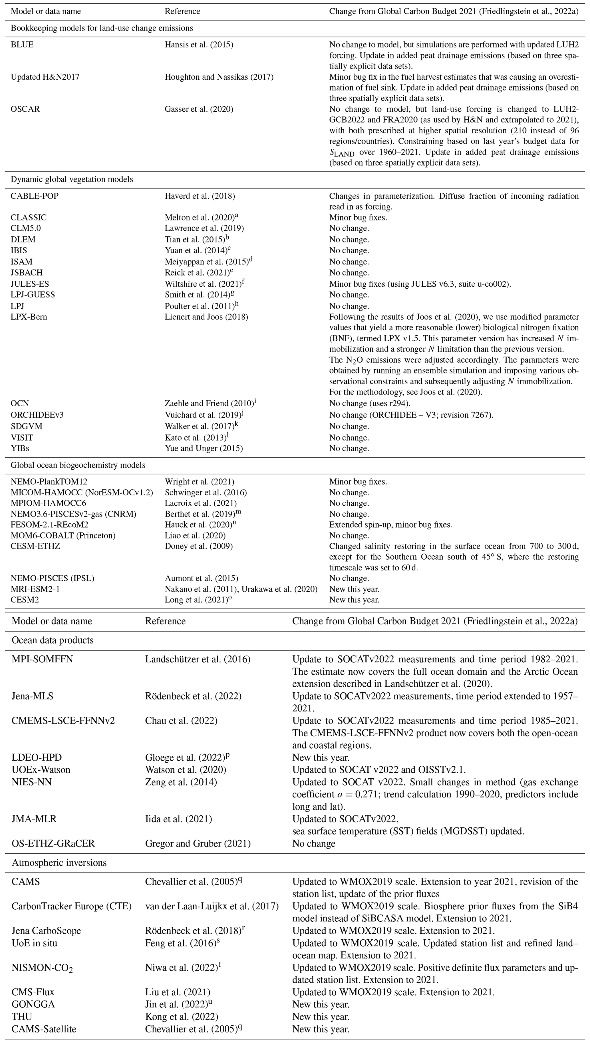
a See also Asaadi et al. (2018). b See also Tian et al. (2011). c The dynamic carbon allocation scheme was presented by Xia et al. (2015). d See also Jain et al. (2013). Soil biogeochemistry is updated based on Shu et al. (2020). e See also Mauritsen et al. (2019). f See also Sellar et al. (2019) and Burton et al. (2019). JULES-ES is the Earth System configuration of the Joint UK Land Environment Simulator as used in the UK Earth System Model (UKESM). g To account for the differences between the derivation of short-wave radiation from CRU cloudiness and DSWRF from CRUJRA, the photosynthesis scaling parameter α was modified (−15 %) to yield similar results. h Compared to published version, decreased LPJ wood harvest efficiency so that 50 % of biomass was removed off-site compared to 85 % used in the 2012 budget. Residue management of managed grasslands increased so that 100 % of harvested grass enters the litter pool. i See also Zaehle et al. (2011). j See also Zaehle and Friend (2010) and Krinner et al. (2005) k See also Woodward and Lomas (2004). l See also Ito and Inatomi (2012). m See also Séférian et al. (2019). n See also Schourup-Kristensen et al. (2014). o See also Yeager et al. (2022). p See also Bennington et al. (2022). q See also Remaud (2018). r See also Rödenbeck et al. (2003). s See also Feng et al. (2009) and Palmer et al. (2019)t See also Niwa et al. (2020)u See also Tian et al. (2014).
2.3.2 The 2022 projection
We provide an assessment of GATM for 2022 based on the monthly calculated global atmospheric CO2 concentration (GLO) through August (Dlugokencky and Tans, 2022), and bias-adjusted Holt–Winters exponential smoothing with additive seasonality (Chatfield, 1978) to project to January 2023. Additional analysis suggests that the first half of the year (the boreal winter–spring–summer transition) shows more interannual variability than the second half of the year (the boreal summer–autumn–winter transition), so that the exact projection method applied to the second half of the year has a relatively smaller impact on the projection of the full year. Uncertainty is estimated from past variability using the standard deviation of the last 5 years of monthly growth rates.
2.4 Ocean CO2 sink
2.4.1 Historical period 1850–2021
The reported estimate of the global ocean anthropogenic CO2 sink SOCEAN is derived as the average of two estimates. The first estimate is derived as the mean over an ensemble of 10 global ocean biogeochemistry models (GOBMs, Tables 4 and A2). The second estimate is obtained as the mean over an ensemble of seven observation-based data products (Tables 4 and A3). An eighth product (Watson et al., 2020) is shown but is not included in the ensemble average as it differs from the other products by adjusting the flux to a cool, salty ocean surface skin (see Appendix C3.1 for a discussion of the Watson product). The GOBMs simulate both the natural and anthropogenic CO2 cycles in the ocean. They constrain the anthropogenic air–sea CO2 flux (the dominant component of SOCEAN) by the transport of carbon into the ocean interior, which is also the controlling factor of present-day ocean carbon uptake in the real world. They cover the full globe and all seasons and were recently evaluated against surface ocean carbon observations, suggesting they are suitable to estimate the annual ocean carbon sink (Hauck et al., 2020). The data products are tightly linked to observations of fCO2 (fugacity of CO2, which equals pCO2 corrected for the non-ideal behaviour of the gas; Pfeil et al., 2013), which carry imprints of temporal and spatial variability, but are also sensitive to uncertainties in gas exchange parameterizations and data sparsity. Their asset is the assessment of interannual and spatial variability (Hauck et al., 2020). We use two further diagnostic ocean models to estimate SOCEAN over the industrial era (1781–1958).
The global fCO2-based flux estimates were adjusted to remove the pre-industrial ocean source of CO2 to the atmosphere of 0.65 GtC yr−1 from river input to the ocean (Regnier et al., 2022) to satisfy our definition of SOCEAN (Hauck et al., 2020). The river flux adjustment was distributed over the latitudinal bands using the regional distribution of Aumont et al. (2001; north: 0.17 GtC yr−1; tropics: 0.16 GtC yr−1; south: 0.32 GtC yr−1), acknowledging that the boundaries of Aumont et al. (2001; namely 20∘ S and 20∘ N) are not consistent with the boundaries otherwise used in the GCB (30∘ S and 30∘ N). A recent study based on one ocean biogeochemical model (Lacroix et al., 2020) suggests that more of the riverine outgassing is located in the tropics than in the Southern Ocean, and hence this regional distribution is associated with a major uncertainty. Anthropogenic perturbations of river carbon and nutrient transport to the ocean are not considered (see Sect. 2.7 and Appendix D3).
We derive SOCEAN from GOBMs by using a simulation (sim A) with historical forcing of climate and atmospheric CO2, accounting for model biases and drift from a control simulation (sim B) with constant atmospheric CO2 and normal-year climate forcing. A third simulation (sim C) with historical atmospheric CO2 increase and normal-year climate forcing is used to attribute the ocean sink to CO2 (sim C minus sim B) and climate (sim A minus sim C) effects. A fourth simulation (sim D; historical climate forcing and constant atmospheric CO2) is used to compare the change in anthropogenic carbon inventory in the interior ocean (sim A minus sim D) to the observational estimate of Gruber et al. (2019) with the same flux components (steady state and non-steady state anthropogenic carbon flux). Data products are adjusted to represent the full ice-free ocean area by a simple scaling approach when coverage is below 99 %. GOBMs and data products fall within the observational constraints over the 1990s (2.2 ± 0.7 GtC yr−1, Ciais et al., 2013) after applying adjustments.
SOCEAN is calculated as the average of the GOBM ensemble mean and data product ensemble mean from 1990 onwards. Prior to 1990, it is calculated as the GOBM ensemble mean plus half of the offset between GOBMs and data product ensemble means over 1990–2001.
We assign an uncertainty of ± 0.4 GtC yr−1 to the ocean sink based on a combination of random (ensemble standard deviation) and systematic uncertainties (GOBM bias in anthropogenic carbon accumulation, previously reported uncertainties in fCO2-based data products; see Appendix C3.3). We assess a medium confidence level to the annual ocean CO2 sink and its uncertainty because it is based on multiple lines of evidence, it is consistent with ocean interior carbon estimates (Gruber et al., 2019, see Sect. 3.5.5) and the interannual variability in the GOBMs, and data-based estimates are largely consistent and can be explained by climate variability. We refrain from assigning a high confidence because of the systematic deviation between the GOBM and data product trends since around 2002. More details on the SOCEAN methodology can be found in Appendix C3.
2.4.2 The 2022 projection
The ocean CO2 sink forecast for the year 2022 is based on the annual historical and estimated 2022 atmospheric CO2 concentration (Dlugokencky and Tans, 2022), the historical and estimated 2022 annual global fossil fuel emissions from this year's carbon budget, and the spring (March, April, May) Oceanic Niño Index (ONI) (NCEP, 2022). Using a non-linear regression approach, i.e. a feed-forward neural network, atmospheric CO2, ONI, and fossil fuel emissions are used as training data to best match the annual ocean CO2 sink (i.e. combined SOCEAN estimate from GOBMs and data products) from 1959 through 2021 from this year's carbon budget. Using this relationship, the 2022 SOCEAN can then be estimated from the projected 2021 input data using the non-linear relationship established during the network training. To avoid overfitting, the neural network was trained with a variable number of hidden neurons (varying between 2–5), and 20 % of the randomly selected training data were withheld for independent internal testing. Based on the best output performance (tested using the 20 % withheld input data), the best performing number of neurons was selected. In a second step, we trained the network 10 times using the best number of neurons identified in step 1 and different sets of randomly selected training data. The mean of the 10 training sequences is considered our best forecast, whereas the standard deviation of the 10 ensembles provides a first-order estimate of the forecast uncertainty. This uncertainty is then combined with the SOCEAN uncertainty (0.4 GtC yr−1) to estimate the overall uncertainty of the 2022 projection.
2.5 Land CO2 sink
2.5.1 Historical period
The terrestrial land sink (SLAND) is thought to be due to the combined effects of fertilization by rising atmospheric CO2 and N inputs on plant growth, as well as the effects of climate change such as the lengthening of the growing season in northern temperate and boreal areas. SLAND does not include land sinks directly resulting from land use and land-use change (e.g. regrowth of vegetation) as these are part of the land-use flux (ELUC), although system boundaries make it difficult to exactly attribute CO2 fluxes on land between SLAND and ELUC (Erb et al., 2013).
SLAND is estimated from the multi-model mean of 16 DGVMs (Table A1). As described in Appendix C.4, DGVM simulations include all climate variability and CO2 effects over land. In addition to the carbon cycle represented in all DGVMs, 11 models also account for the nitrogen cycle and hence can include the effect of N inputs on SLAND. The DGVM estimate of SLAND does not include the export of carbon to aquatic systems or its historical perturbation, which is discussed in Appendix D3. See Appendix C4 for DGVM evaluation and uncertainty assessment for SLAND using the International Land Model Benchmarking system (ILAMB; Collier et al., 2018). More details on the SLAND methodology can be found in Appendix C4.
2.5.2 The 2022 projection
Like for the ocean forecast, the land CO2 sink (SLAND) forecast is based on the annual historical and estimated 2022 atmospheric CO2 concentration (Dlugokencky and Tans, 2021), historical and estimated 2022 annual global fossil fuel emissions from this year's carbon budget, and the summer (June, July, August) ONI (NCEP, 2022). All training data are again used to best match SLAND from 1959 through 2021 from this year's carbon budget using a feed-forward neural network. To avoid overfitting, the neural network was trained with a variable number of hidden neurons (varying between 2–15), larger than for SOCEAN prediction due to the stronger land carbon interannual variability. As done for SOCEAN, a pre-training selects the optimal number of hidden neurons based on 20 % withheld input data, and in a second step, an ensemble of 10 forecasts is produced to provide the mean forecast plus uncertainty. This uncertainty is then combined with the SLAND uncertainty for 2021 (0.9 GtC yr−1) to estimate the overall uncertainty of the 2022 projection.
2.6 The atmospheric perspective
The world-wide network of in situ atmospheric measurements and satellite-derived atmospheric CO2 column (xCO2) observations put a strong constraint on changes in the atmospheric abundance of CO2. This is true globally (hence our large confidence in GATM) but also regionally in regions with sufficient observational density found mostly in the extratropics. This allows atmospheric inversion methods to constrain the magnitude and location of the combined total surface CO2 fluxes from all sources, including fossil and land-use change emissions and land and ocean CO2 fluxes. The inversions assume EFOS to be well known, and they solve for the spatial and temporal distribution of land and ocean fluxes from the residual gradients of CO2 between stations that are not explained by fossil fuel emissions. By design, such systems thus close the carbon balance (BIM=0) and thus provide an additional perspective on the independent estimates of the ocean and land fluxes.
This year's release includes nine inversion systems that are described in Table A4. Each system is rooted in Bayesian inversion principles but uses different methodologies. These differences concern the selection of atmospheric CO2 data or xCO2, and the choice of a priori fluxes to refine. They also differ in spatial and temporal resolution, assumed correlation structures, and mathematical approach of the models (see references in Table A4 for details). Importantly, the systems use a variety of transport models, which was demonstrated to be a driving factor behind differences in atmospheric inversion-based flux estimates and specifically their distribution across latitudinal bands (Gaubert et al., 2019; Schuh et al., 2019). Four inversion systems (CAMS-FT21r2, CMS-flux, GONGGA, THU) used satellite xCO2 retrievals from GOSAT and/or OCO-2, scaled to the WMO 2019 calibration scale. One inversion this year (CMS-Flux) used these xCO2 data sets in addition to the in situ observational CO2 mole fraction records.
The original products delivered by the inverse modellers were modified to facilitate the comparison to the other elements of the budget, specifically on two accounts: (1) global total fossil fuel emissions, including cement carbonation CO2 uptake, and (2) riverine CO2 transport. Details are given below. We note that with these adjustments the inverse results no longer represent the net atmosphere–surface exchange over land and ocean areas as sensed by atmospheric observations. Instead, for land, they become the net uptake of CO2 by vegetation and soils that is not exported by fluvial systems, similar to the DGVM estimates. For oceans, they become the net uptake of anthropogenic CO2, similar to the GOBM estimates.
The inversion systems prescribe global fossil fuel emissions based on the GCP's Gridded Fossil Emissions Dataset versions 2022.1 or 2022.2 (GCP-GridFED; Jones et al., 2022), which are updates to GCP-GridFEDv2021 presented by Jones et al. (2021). GCP-GridFEDv2022 scales gridded estimates of CO2 emissions from EDGARv4.3.2 (Janssens-Maenhout et al., 2019) within national territories to match national emissions estimates provided by the GCB for the years 1959–2021, which were compiled following the methodology described in Sect. 2.1. Small differences between the systems due to, for instance, regridding to the transport model resolution or use of different GridFED versions with different cement carbonation sinks (which were only present starting with GridFEDv2022.1) are adjusted in the latitudinal partitioning we present to ensure agreement with the estimate of EFOS in this budget. We also note that the ocean fluxes used as prior by six out of the nine inversions are part of the suite of the ocean process models or fCO2 data products listed in Sect. 2.4. Although these fluxes are further adjusted by the atmospheric inversions, it makes the inversion estimates of the ocean fluxes not completely independent of SOCEAN assessed here.
To facilitate comparisons to the independent SOCEAN and SLAND, we used the same corrections for transport and outgassing of carbon transported from land to ocean, as has been done for the observation-based estimates of SOCEAN (see Appendix C3).
The atmospheric inversions are evaluated using vertical profiles of atmospheric CO2 concentrations (Fig. B4). More than 30 aircraft programmes over the globe, either regular programmes or repeated surveys over at least 9 months (except for Southern Hemisphere, SH, programmes), have been used to assess system performance (with space–time observational coverage sparse in the SH and tropics, and denser in Northern Hemisphere, NH, mid-latitudes; Table A6). The nine systems are compared to the independent aircraft CO2 measurements between 2 and 7 km above sea level between 2001 and 2021. Results are shown in Fig. B4 and discussed in Appendix C5.2
With a relatively small ensemble (N=9) of systems that moreover share some a priori fluxes used with one another, or with the process-based models, it is difficult to justify using their mean and standard deviation as a metric for uncertainty across the ensemble. We therefore report their full range (min–max) without their mean. More details on the atmospheric inversions methodology can be found in Appendix C5.
2.7 Processes not included in the global carbon budget
The contribution of anthropogenic CO and CH4 to the global carbon budget is not fully accounted for in Eq. (1) and is described in Appendix D1. The contributions to CO2 emissions of decomposition of carbonates not accounted for is described in Appendix D2. The contribution of anthropogenic changes in river fluxes is conceptually included in Eq. (1) in SOCEAN and in SLAND, but it is not represented in the process models used to quantify these fluxes. This effect is discussed in Appendix D3. Similarly, the loss of additional sink capacity from reduced forest cover is missing in the combination of approaches used here to estimate both land fluxes (ELUC and SLAND) and its potential effect is discussed and quantified in Appendix D4.
For each component of the global carbon budget, we present results for three different time periods: the full historical period, from 1850 to 2021, the 6 decades in which we have atmospheric concentration records from Mauna Loa (1960–2021); a specific focus on the last year (2021); and the projection for the current year (2022). Subsequently, we assess the combined constraints from the budget components (often referred to as a bottom-up budget) against the top-down constraints from inverse modelling of atmospheric observations. We do this for the global balance of the last decade, as well as for a regional breakdown of land and ocean sinks by broad latitude bands.
3.1 Fossil CO2 emissions
3.1.1 Historical period 1850–2021
Cumulative fossil CO2 emissions for 1850–2021 were 465 ± 25 GtC, including the cement carbonation sink (Fig. 3, Table 8, all cumulative numbers are rounded to the nearest 5 GtC).
In this period, 46 % of fossil CO2 emissions came from coal, 35 % from oil, 15 % from natural gas, 3 % from decomposition of carbonates, and 1 % from flaring.
In 1850, the UK contributed 62 % of global fossil CO2 emissions. In 1891 the combined cumulative emissions of the current members of the European Union reached and subsequently surpassed the level of the UK. Since 1917, US cumulative emissions have been the largest. Over the entire period 1850–2021, US cumulative emissions amounted to 115 GtC (24 % of world total), the EU's to 80 GtC (17 %), and China's to 70 GtC (14 %).
In addition to the estimates of fossil CO2 emissions that we provide here (see Sect. 2), there are three additional global data sets with long time series that include all sources of fossil CO2 emissions: CDIAC-FF (Gilfillan and Marland, 2021), CEDS version v_2021_04_21 (Hoesly et al., 2018; O'Rourke et al., 2021), and PRIMAP-hist version 2.3.1 (Gütschow et al., 2016, 2021), although these data sets are not entirely independent of each other (Andrew, 2020a). CDIAC-FF has the lowest cumulative emissions over 1750–2018 at 437 GtC, GCP has 443 GtC, CEDS 445 GtC, PRIMAP-hist TP 453 GtC, and PRIMAP-hist CR 455 GtC. CDIAC-FF excludes emissions from lime production, while neither CDIAC-FF nor GCP explicitly include emissions from international bunker fuels prior to 1950. CEDS has higher emissions from international shipping in recent years, while PRIMAP-hist has higher fugitive emissions than the other data sets. However, in general these four data sets are in relative agreement as to total historical global emissions of fossil CO2.
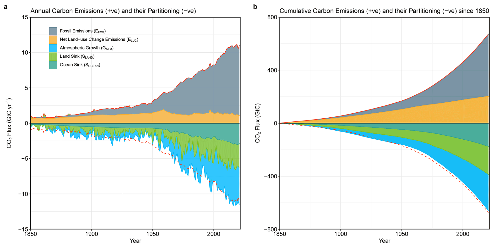
Figure 3Combined components of the global carbon budget illustrated in Fig. 2 as a function of time for fossil CO2 emissions (EFOS, including a small sink from cement carbonation; grey) and emissions from land-use change (ELUC; brown), as well as their partitioning among the atmosphere (GATM; cyan), ocean (SOCEAN; blue), and land (SLAND; green). Panel (a) shows annual estimates of each flux, and panel (b) shows the cumulative flux (the sum of all prior annual fluxes) since the year 1850. The partitioning is based on nearly independent estimates from observations (for GATM) and from process model ensembles constrained by data (for SOCEAN and SLAND) and does not exactly add up to the sum of the emissions, resulting in a budget imbalance (BIM), which is represented by the difference between the bottom red line (mirroring total emissions) and the sum of carbon fluxes in the ocean, land, and atmosphere reservoirs. All data are in GtC yr−1 (a) and GtC (b). The EFOS estimate is based on a mosaic of different data sets, and has an uncertainty of ±5 % (±1σ). The ELUC estimate is from three bookkeeping models (Table 4) with uncertainty of ±0.7 GtC yr−1. The GATM estimates prior to 1959 are from Joos and Spahni (2008) with uncertainties equivalent to about ±0.1–0.15 GtC yr−1 and from Dlugokencky and Tans (2022) since 1959 with uncertainties of about +-0.07 GtC yr−1 during 1959–1979 and ± 0.02 GtC yr−1 since 1980. The SOCEAN estimate is the average from Khatiwala et al. (2013) and DeVries (2014) with uncertainty of about ±30 % prior to 1959, and the average of an ensemble of models and an ensemble of fCO2 data products (Table 4) with uncertainties of about ±0.4 GtC yr−1 since 1959. The SLAND estimate is the average of an ensemble of models (Table 4) with uncertainties of about ±1 GtC yr−1. See the text for more details of each component and their uncertainties.
3.1.2 Recent period 1960–2021
Global fossil CO2 emissions, EFOS (including the cement carbonation sink), have increased every decade from an average of 3.0 ± 0.2 GtC yr−1 for the decade of the 1960s to an average of 9.6 ± 0.5 GtC yr−1 during 2012–2021 (Table 6, Figs. 2 and 5). The growth rate in these emissions decreased between the 1960s and the 1990s, from 4.3 % per year in the 1960s (1960–1969), 3.2 % per year in the 1970s (1970–1979), 1.6 % per year in the 1980s (1980–1989), and 0.9 % per year in the 1990s (1990–1999). After this period, the growth rate began increasing again in the 2000s at an average growth rate of 3.0 % per year, decreasing to 0.5 % per year for the last decade (2012–2021). China's emissions increased by +1.5 % per year on average over the last 10 years, dominating the global trend, and India's emissions increased by +3.8 % per year, while emissions decreased in EU27 by −1.8 % per year and in the USA by −1.1 % per year. Figure 6 illustrates the spatial distribution of fossil fuel emissions for the 2012–2021 period.
EFOS includes the uptake of CO2 by cement via carbonation, which has increased with increasing stocks of cement products from an average of 20 MtC yr−1 (0.02 GtC yr−1) in the 1960s to an average of 200 MtC yr−1 (0.2 GtC yr−1) during 2012–2021 (Fig. 5).
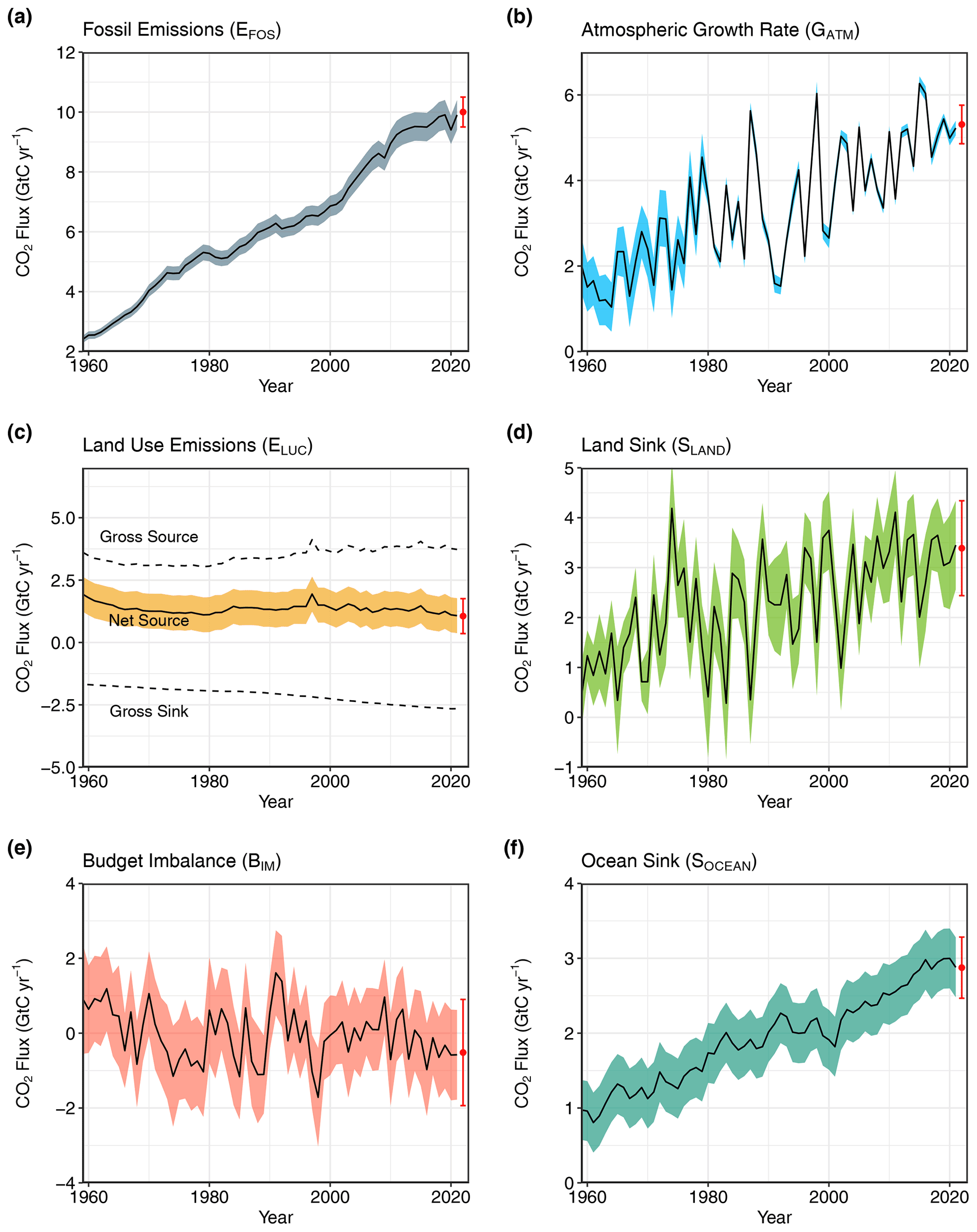
Figure 4Components of the global carbon budget and their uncertainties as a function of time, presented individually for (a) fossil CO2 and cement carbonation emissions (EFOS), (b) growth rate in atmospheric CO2 concentration (GATM), (c) emissions from land-use change (ELUC), (d) the land CO2 sink (SLAND), (e) the ocean CO2 sink (SOCEAN), and (f) the budget imbalance that is not accounted for by the other terms. Positive values of SLAND and SOCEAN represent a flux from the atmosphere to land or the ocean. All data are in GtC yr−1 with the uncertainty bounds representing ±1 standard deviation in shaded colour. Data sources are as in Fig. 3. The red dots indicate our projections for the year 2022, and the red error bars the uncertainty in the projections (see Sect. 2).
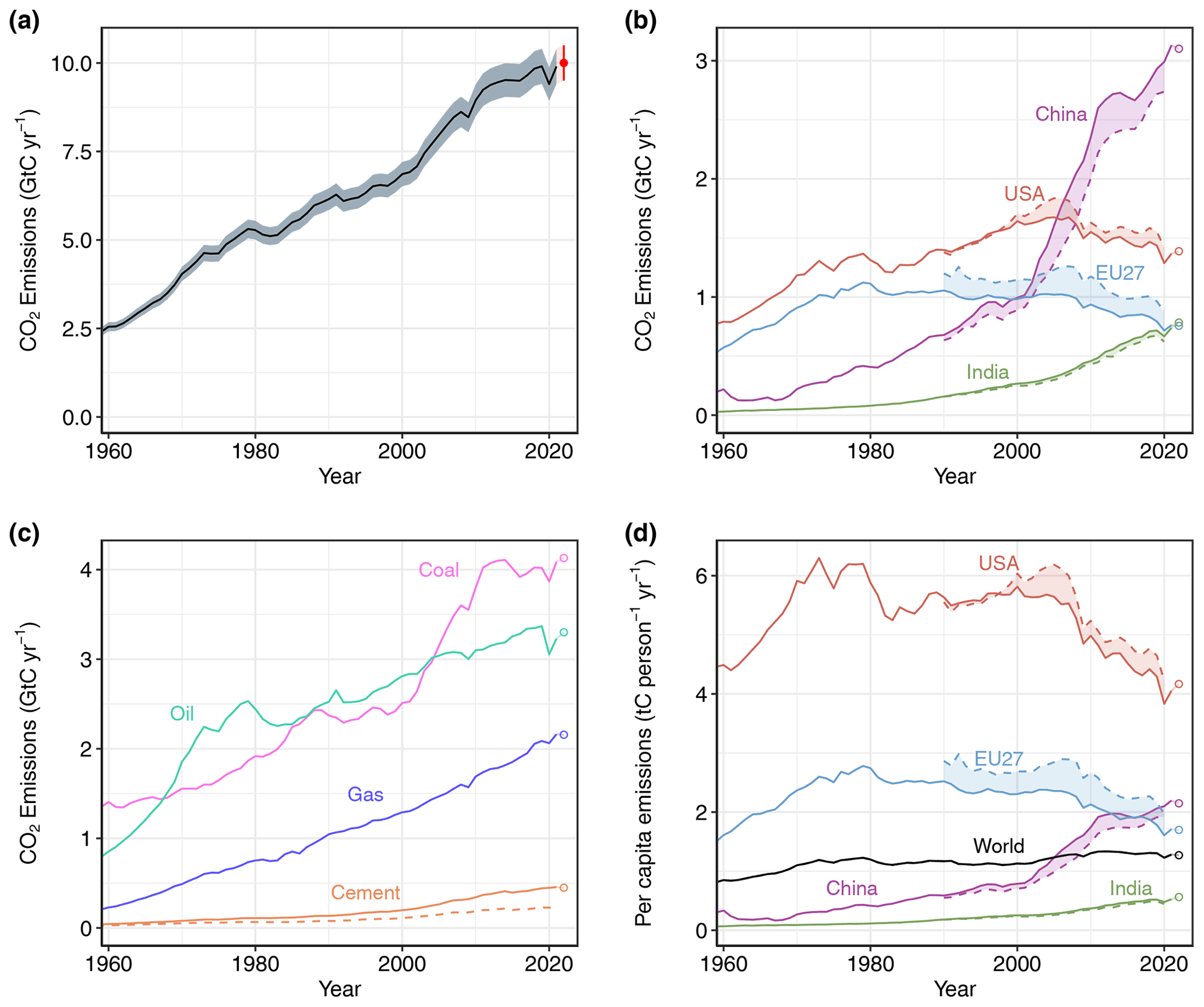
Figure 5Fossil CO2 emissions for (a) the globe, including an uncertainty of ± 5 % (grey shading) and a projection through the year 2022 (red dot and uncertainty range); (b) territorial (solid lines) and consumption (dashed lines) emissions for the top three country emitters (USA, China, India) and for the European Union (EU27); (c) global emissions by fuel type, including coal, oil, gas, cement, and cement minus cement carbonation (dashed); and (d) per capita emissions for the world and for the large emitters, as in panel (b). Territorial emissions are primarily from a draft update of Gilfillan and Marland (2021), with the exception of the national data for Annex I countries for 1990–2020, which are reported to the UNFCCC as detailed in the text, as well as some improvements in individual countries, and are extrapolated forward to 2021 using BP Energy Statistics. Consumption-based emissions are updated from Peters et al. (2011b). See Sect. 2.1 and Appendix C1 for details about the calculations and data sources.
3.1.3 Final year 2021
Global fossil CO2 emissions were 5.1 % higher in 2021 than in 2020 because of the global rebound from the worst of the COVID-19 pandemic, with an increase of 0.5 GtC to reach 9.9 ± 0.5 GtC (including the cement carbonation sink) in 2021 (Fig. 5), distributed among coal (41 %), oil (32 %), natural gas (22 %), cement (5 %), and others (1 %). Compared to the previous year, 2021 emissions from coal, oil, and gas increased by 5.7 %, 5.8 %, and 4.8 %, respectively, while emissions from cement increased by 2.1 %. All growth rates presented are adjusted for the leap year unless stated otherwise.
In 2021, the largest absolute contributions to global fossil CO2 emissions were from China (31 %), the USA (14 %), the EU27 (8 %), and India (7 %). These four regions account for 59 % of global CO2 emissions, while the rest of the world contributed 41 %, including international aviation and marine bunker fuels (2.8 % of the total). Growth rates for these countries from 2020 to 2021 were 3.5 % (China), 6.2 % (USA), 6.8 % (EU27), and 11.1 % (India), with +4.5 % for the rest of the world. The per capita fossil CO2 emissions in 2021 were 1.3 tC per person per year for the globe and were 4.0 (USA), 2.2 (China), 1.7 (EU27), and 0.5 (India) tC per person per year for the four highest-emitting countries (Fig. 5).
The post-COVID-19 rebound in emissions of 5.1 % in 2021 is close to the projected increase of 4.8 % published in Friedlingstein et al. (2022a) (Table 7). Of the regions, the projection for the “rest of world” region was least accurate (off by −1.3 %), largely because of poorly projected emissions from international transport (bunker fuels), which were subject to very large changes during this period.
3.1.4 Year 2022 projection
Globally, we estimate that global fossil CO2 emissions (including cement carbonation) will grow by 1.0 % in 2022 (0.1 % to 1.9 %) to 10.0 GtC (36.6 GtCO2), exceeding their 2019 emission levels of 9.9 GtC (36.3 GtCO2). Global increase in 2022 emissions per fuel types are projected to be +1 % (range 0.2 % to 1.8 %) for coal, +2.2 % (range 1.1 % to 3.3 %) for oil, −0.2 % (range −1.1 % to 0.7 %) for natural gas, and −1.6 % (range −3.7 % to −0.5 %) for cement.
For China, projected fossil emissions in 2022 are expected to decline by 0.9 % (range −2.3 % to +0.4 %) compared with 2021 emissions, bringing 2022 emissions for China to around 3.1 GtC yr−1 (11.4 GtCO2 yr−1). Changes in fuel-specific projections for China are +0.1 % for coal, −2.8 % for oil, −1.1 % for natural gas, and −7.0 % for cement.
For the USA, the Energy Information Administration (EIA) emissions projection for 2022 combined with cement clinker data from USGS gives an increase of 1.5 % (range −1 % to +4 %) compared to 2021, bringing 2022 USA emissions to around 1.4 GtC yr−1 (5.1 GtCO2 yr−1). This is based on separate projections for coal of −4.6 %, oil of +2 %, natural gas of +4.7 %, and cement of +1.2 %.
For the European Union, our projection for 2022 is for a decline of 0.8 % (range −2.8 % to +1.2 %) over 2021, with 2022 emissions around 0.8 GtC yr−1 (2.8 GtCO2 yr−1). This is based on separate projections for coal of +6.7 %, oil of +0.9 %, and natural gas of −10.0 %, while cement remains unchanged.
For India, our projection for 2022 is an increase of 6 % (range of 3.9 % to 8 %) over 2021, with 2022 emissions around 0.8 GtC yr−1 (2.9 GtCO2 yr−1). This is based on separate projections for coal of +5.0 %, oil of +10.0 %, natural gas of −4.0 %, and cement of +10.0 %.
For the rest of the world, the expected growth rate for 2022 is 1.7 % (range 0.1 % to 3.3 %). The fuel-specific projected 2022 growth rates for the rest of the world are: +1.6 % for coal, +3.1 % for oil, −0.1 % for natural gas, +3 % for cement.
3.2 Emissions from land-use changes
3.2.1 Historical period 1850–2021
Cumulative CO2 emissions from land-use changes (ELUC) for 1850–2021 were 205 ± 60 GtC (Table 8; Fig. 3; Fig. 14). The cumulative emissions from ELUC show a large spread among individual estimates of 140 GtC (updated H&N2017), 280 GtC (BLUE), and 190 GtC (OSCAR) for the three bookkeeping models and a similar wide estimate of 185 ± 60 GtC for the DGVMs (all cumulative numbers are rounded to the nearest 5 GtC). These estimates are broadly consistent with indirect constraints from vegetation biomass observations, giving a cumulative source of 155 ± 50 GtC over the 1901–2012 period (Li et al., 2017). However, given the large spread, a best estimate is difficult to ascertain.
3.2.2 Recent period 1960–2021
In contrast to growing fossil emissions, CO2 emissions from land use, land-use change, and forestry have remained relatively constant over the 1960–1999 period but show a slight decrease of about 0.1 GtC per decade since the 1990s, reaching 1.2 ± 0.7 GtC yr−1 for the 2012–2021 period (Table 6) but with large spread across estimates (Table 5, Fig. 7). Different from the bookkeeping average, the DGVM model average grows slightly larger over the 1970–2021 period and shows no sign of decreasing emissions in the recent decades (Table 5, Fig. 7). This is, however, expected as DGVM-based estimates include the loss of additional sink capacity, which grows with time, while the bookkeeping estimates do not (Appendix D4).
Table 5Comparison of results from the bookkeeping method and budget residuals with results from the DGVMs and inverse estimates for different periods, the last decade, and the last year available. All values are in GtC yr−1. See Fig. 7 for an explanation of the bookkeeping component fluxes. The DGVM uncertainties represent ±1σ of the decadal or annual (for 2021) estimates from the individual DGVMs; for the inverse systems the range of available results is given. All values are rounded to the nearest 0.1 GtC and therefore columns do not necessarily add to zero.

∗ Estimates are adjusted for the pre-industrial influence of river fluxes and the cement carbonation sink and are also adjusted to common EFOS (Sect. 2.6). The ranges given include varying numbers (in parentheses) of inversions in each decade (Table A4).
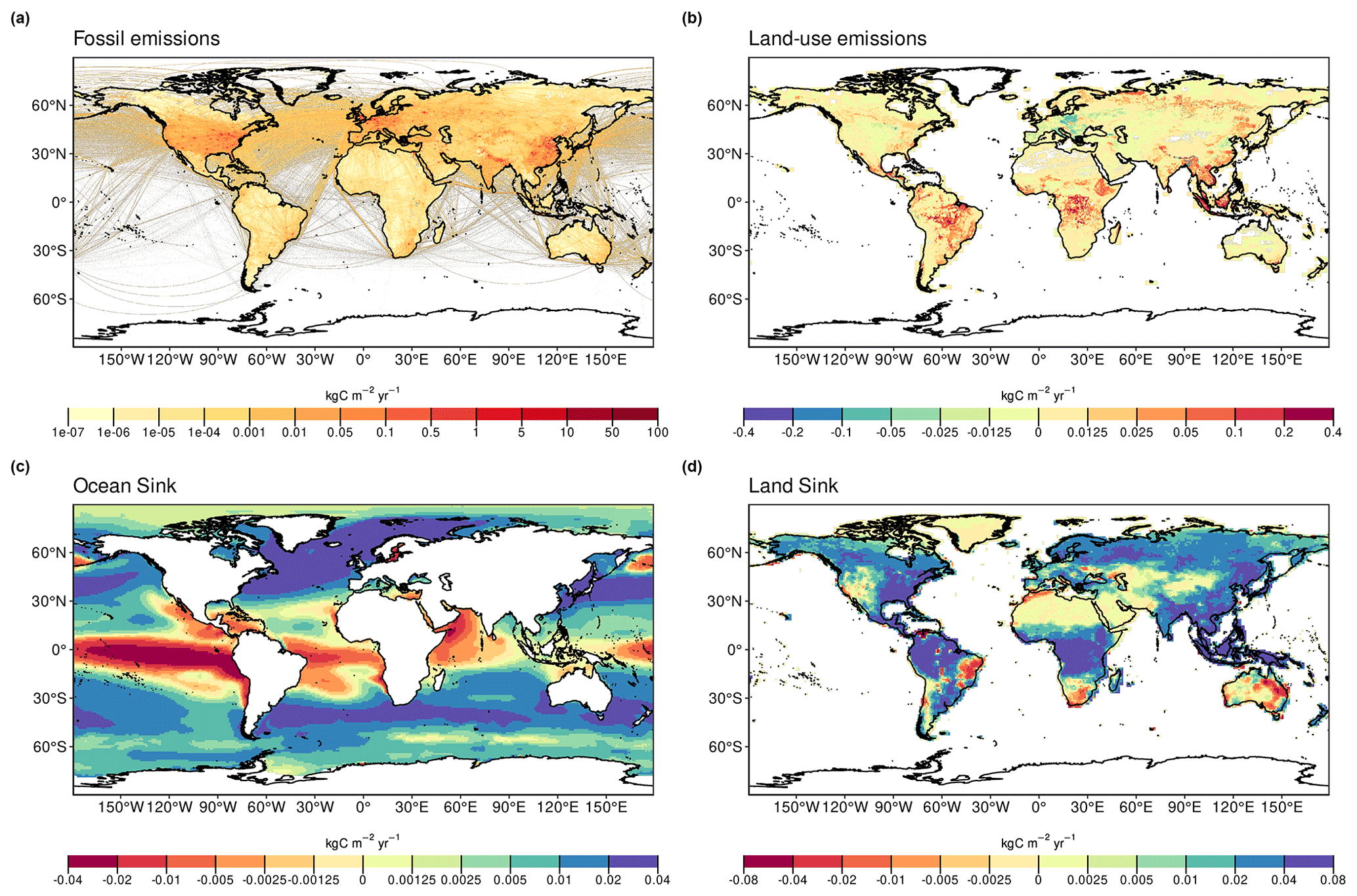
Figure 6The 2012–2021 decadal mean components of the global carbon budget, presented for (a) fossil CO2 emissions (EFOS), (b) land-use change emissions (ELUC), (c) the ocean CO2 sink (SOCEAN), and (d) the land CO2 sink (SLAND). Positive values for EFOS and ELUC represent a flux to the atmosphere, whereas positive values of SOCEAN and SLAND represent a flux from the atmosphere to the ocean or the land. In all panels, yellow and red (green and blue) colours represent a flux from (into) the land and ocean to (from) the atmosphere. All units are in kgC m−2 yr−1. Note the different scales in each panel. EFOS data shown is from GCP-GridFEDv2022.2. ELUC data shown are only from BLUE as the updated H&N2017 and OSCAR do not resolve gridded fluxes. SOCEAN data shown are the average of GOBMs and data product means using GOBM simulation A with no adjustment for bias or drift applied to the gridded fields (see Sect. 2.4). SLAND data shown are the average of DGVMs for simulation S2 (see Sect. 2.5).
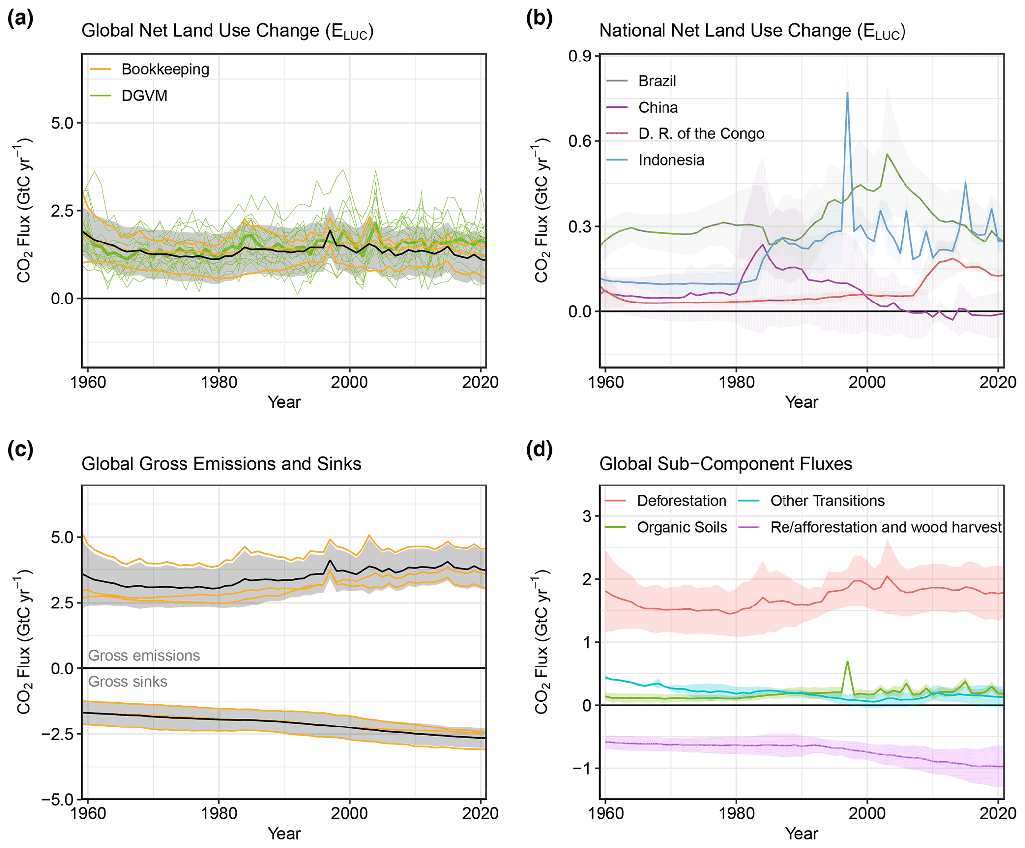
Figure 7Net CO2 exchanges between the atmosphere and the terrestrial biosphere related to land-use change. (a) Net CO2 emissions from land-use change (ELUC) with estimates from the three bookkeeping models (yellow lines) and the budget estimate (black with ±1σ uncertainty), which is the average of the three bookkeeping models. Estimates from individual DGVMs (narrow green lines) and the DGVM ensemble mean (thick green line) are also shown. (b) Net CO2 emissions from land-use change from the four countries with largest cumulative emissions since 1959. Values shown are the average of the three bookkeeping models, with shaded regions as ±1σ uncertainty. (c) CO2 gross sinks (negative, from regrowth after agricultural abandonment and wood harvesting) and gross sources (positive, from decaying material left dead on site, products after clearing of natural vegetation for agricultural purposes, wood harvesting, and, for BLUE, degradation from primary to secondary land through usage of natural vegetation as rangeland and from emissions from peat drainage and peat burning). Values are shown for the three bookkeeping models (yellow lines) and for their average (black with ±1σ uncertainty). The sum of the gross sinks and sources is ELUC shown in panel (a). (d) Sources and sinks aggregated into four components that contribute to the net fluxes of CO2, including (i) gross sources from deforestation; (ii) afforestation, reafforestation, and wood harvest (i.e. the net flux on forest lands comprising slash and product decay following wood harvest and sinks due to regrowth after wood harvest or after abandonment, including reforestation and abandonment as parts of shifting cultivation cycles); (iii) emissions from organic soils (peat drainage and peat fire); and (iv) sources and sinks related to other land-use transitions. The scale of the fluxes shown is smaller than in panel (c) because the substantial gross sources and sinks from wood harvesting are accounted for as net flux under (ii). The sum of the component fluxes is ELUC shown in panel (a).
ELUC is a net term of various gross fluxes, which comprise emissions and removals. Gross emissions on average over the 1850–2021 period are 2 (BLUE, OSCAR) to 3 (updated H&N2017) times larger than the net ELUC emissions. Gross emissions show a moderate increase from an average of 3.2 ± 0.9 GtC yr−1 for the decade of the 1960s to an average of 3.8 ± 0.7 GtC yr−1 during 2012–2021 (Fig. 7). Increases in gross removals, from 1.8 ± 0.4 GtC yr−1 for the 1960s to 2.6 ± 0.4 GtC yr−1 for 2012–2021, were slightly larger than the increase in gross emissions. Since the processes behind gross removals, foremost forest regrowth and soil recovery, are all slow, while gross emissions include a large instantaneous component, short-term changes in land-use dynamics, such as a temporary decrease in deforestation, influences gross emissions dynamics more than gross removal dynamics. It is these relative changes to each other that explain the small decrease in net ELUC emissions over the last 2 decades and the last few years. Gross fluxes often differ more across the three bookkeeping estimates than net fluxes, which is expected due to different process representation; in particular, treatment of shifting cultivation, which increases both gross emissions and removals, differs across models.
There is a smaller decrease in net CO2 emissions from land-use change in the last few years (Fig. 7) than in last year's estimate (Friedlingstein et al., 2021), which places our updated estimates between last year's estimate and the estimate from the GCB2020 (Friedlingstein et al., 2020). This change is principally attributable to changes in ELUC estimates from BLUE and OSCAR, which relate to improvements in the underlying land-use forcing (see Appendix C2.2 for details). These changes address issues identified with last year's land-use forcing (see Friedlingstein et al., 2022a) and remove or attenuate several emission peaks in Brazil and the Democratic Republic of the Congo and lead to higher net emissions in Brazil in the last decades compared to last year's global carbon budget (the emissions averaged over the three bookkeeping models for Brazil for the 2011–2020 period were 168 MtC yr−1 in GCB2021 as compared to 289 MtC yr−1 in GCB2022). A remaining caveat is that global land-use change data for model input does not capture forest degradation, which often occurs on small scale or without forest cover changes easily detectable from remote sensing and poses a growing threat to forest area and carbon stocks that may surpass deforestation effects (e.g. Matricardi et al., 2020; Qin et al., 2021). While independent pan-tropical or global estimates of vegetation cover dynamics or carbon stock changes based on satellite remote sensing have become available in recent years, a direct comparison to our estimates is not possible, most importantly because satellite-based estimates usually do not distinguish between anthropogenic drivers and natural forest cover losses (e.g. from drought or natural wildfires) (Pongratz et al., 2021).
We additionally separate the net ELUC into four component fluxes to gain further insight into the drivers of emissions: deforestation, afforestation, reafforestation, and wood harvest (i.e. all fluxes on forest lands); emissions from organic soils (i.e. peat drainage and peat fires); and fluxes associated with all other transitions (Fig. 7; Sect. C2.1). On average over the 2012–2021 period and over the three bookkeeping estimates, fluxes from deforestation amount to 1.8 ± 0.4 GtC yr−1, and from afforestation, reafforestation, and wood harvest fluxes amount to −0.9 ± 0.3 GtC yr−1 (Table 5). Emissions from organic soils (0.2 ± 0.1 GtC yr−1) and the net flux from other transitions (0.2 ± 0.1 GtC yr−1) are substantially less important globally. Deforestation is thus the main driver of global gross sources. The relatively small deforestation flux (1.8 ± 0.4 GtC yr−1) in comparison to the gross emission estimate above (3.8 ± 0.7 GtC yr−1) is explained by the fact that emissions associated with wood harvesting do not count as deforestation as they do not change the land cover. This split into component fluxes clarifies the potential for emission reduction and carbon dioxide removal: the emissions from deforestation could be halted (largely) without compromising carbon uptake by forests and would contribute to emissions reduction. By contrast, reducing wood harvesting would have limited potential to reduce emissions as it would be associated with less forest regrowth; sinks and sources cannot be decoupled here. Carbon dioxide removal in forests could instead be increased by afforestation and reafforestation.
Overall, the highest land-use emissions occur in the tropical regions of all three continents. The top three emitters (both cumulatively 1959–2021 and on average over 2012–2021) are Brazil (in particular the Amazon Arc of Deforestation), Indonesia, and the Democratic Republic of the Congo, with these three countries contributing 0.7 GtC yr−1 or 58 % of the global total land-use emissions (average over 2012–2021) (Fig. 6b). This is related to massive expansion of cropland, particularly in the last few decades in Latin America, Southeast Asia, and sub-Saharan Africa (Hong et al., 2021), a substantial part of which has been for export of agricultural products (Pendrill et al., 2019). Emission intensity is high in many tropical countries, particularly in Southeast Asia, due to high rates of land conversion in regions of carbon-dense and often still pristine undegraded natural forests (Hong et al., 2021). Emissions are further increased by peat fires in equatorial Asia (GFED4s, van der Werf et al., 2017). Uptake due to land-use change occurs partly due to expanding forest area as a consequence of the forest transition in the 19th and 20th centuries and the subsequent regrowth of forest, particularly in Europe (Fig. 6b) (Mather, 2001; McGrath et al., 2015).
While the mentioned patterns are supported by independent literature and robust, we acknowledge that model spread is substantially larger at regional rather than global levels, as has been shown for bookkeeping models (Bastos et al., 2021) and DGVMs (Obermeier et al., 2021). Assessments for individual regions will be performed as part of REgional Carbon Cycle Assessment and Processes (RECCAP2; Ciais et al., 2022) or already exist for selected regions (e.g. for Europe by Petrescu et al., 2020; for Brazil by Rosan et al., 2021; and for eight selected countries and regions in comparison to inventory data by Schwingshackl et al., 2022).
National GHG inventory data (NGHGI) under the LULUCF sector or data submitted by countries to FAOSTAT differ from the global models' definition of ELUC that we adopt here in that the natural fluxes (SLAND) are counted towards ELUC when they occur on managed land in the NGHGI reporting (Grassi et al., 2018). In order to compare our results to the NGHGI approach, we perform a re-mapping of our ELUC estimates by adding SLAND in managed forest from the DGVM simulations (following Grassi et al., 2021) to the bookkeeping ELUC estimate (see Appendix C2.3). For the 2012–2021 period, we estimate that 1.8 GtC yr−1 of SLAND occurred in managed forests and is then reallocated to ELUC here, as has been done in the NGHGI method. By doing so, our mean estimate of ELUC is reduced from a source of 1.2 GtC to a sink of 0.6 GtC, which is very similar to the NGHGI estimate of a 0.5 GtC sink (Table 9). The re-mapping approach has been shown to also be generally applicable for country-level data (Grassi et al., 2022b; Schwingshackl et al., 2022). Country-level analysis suggests, e.g. that the bookkeeping mean estimates higher deforestation emissions than the national report in Indonesia but estimates less CO2 removal by afforestation than the national report in China. The fraction of the natural CO2 sinks that the NGHGI estimates include differs substantially across countries, related to varying proportions of managed vs. all forest areas (Schwingshackl et al., 2022). Comparing ELUC and NGHGI on the basis of the four component fluxes (Grassi et al., 2022b), we find that NGHGI deforestation emissions are reported to be smaller than the bookkeeping estimate (1.1 GtC yr−1 averaged over 2012–2021). A reason for this lies in the fact that country reports do not (fully) capture the carbon flux consequences of shifting cultivation. Conversely, carbon uptake in forests (afforestation, reafforestation, and forestry) is substantially larger than the bookkeeping estimate (1.75 GtC yr−1 averaged over 2012–2021), owing to the inclusion of natural CO2 fluxes on managed land in the NGHGI. Emissions from organic soils and the net flux from other transitions are similar to the estimates based on the bookkeeping approach and the external peat drainage and burning data sets. Though estimates between NGHGI, FAOSTAT, individual process-based models, and the mapped budget still differ in value and need further analysis, the approach taken here provides a possibility to relate the global models' and NGHGI approach to each other routinely and thus link the anthropogenic carbon budget estimates of land CO2 fluxes directly to the Global Stocktake as part of UNFCCC Paris Agreement.
3.2.3 Final year 2021
The global CO2 emissions from land-use change are estimated as 1.1 ± 0.7 GtC in 2021, similar to the 2020 estimate. However, confidence in the annual change remains low.
Land-use change and related emissions may have been affected by the COVID-19 pandemic (e.g. Poulter et al., 2021). During the period of the pandemic, environmental protection policies and their implementation may have been weakened in Brazil (Vale et al., 2021). In other countries monitoring capacities and legal enforcement of measures to reduce tropical deforestation have also been reduced due to budget restrictions of environmental agencies or the impairments of ground-based monitoring intended to prevent land grabs and tenure conflicts (Brancalion et al., 2020; Amador-Jiménez et al., 2020). Effects of the pandemic on trends in fire activity or forest cover changes are hard to separate from those of general political developments and environmental changes, and the long-term consequences of disruptions in agricultural and forestry economic activities (e.g. Gruère and Brooks, 2021; Golar et al., 2020; Beckman and Countryman, 2021) remain to be seen. Overall, there is limited evidence so far that COVID-19 was a key driver of changes in LULUCF emissions at a global scale. Impacts vary across countries and deforestation-curbing and enhancing factors may partly compensate each other (Wunder et al., 2021).
3.2.4 Year 2022 projection
In Indonesia, peat fire emissions are very low, potentially related to a relatively wet dry season (GFED4.1s, van der Werf et al., 2017). In South America, the trajectory of tropical deforestation and degradation fires resembles the long-term average; global emissions from tropical deforestation and degradation fires were estimated to be 206 TgC by 14 October 2020. (GFED4.1s, van der Werf et al., 2017). Our preliminary estimate of ELUC for 2022 is substantially lower than the 2012–2021 average, which saw years of anomalously dry conditions in Indonesia and high deforestation fires in South America (Friedlingstein et al., 2022a). Based on the fire emissions until 14 October, we expect ELUC emissions of around 1.1 GtC in 2022. Note that although our extrapolation is based on tropical deforestation and degradation fires, degradation attributable to selective logging, edge effects, or fragmentation will not be captured. Further, deforestation and fires in deforestation zones may become more disconnected, partly due changes in legislation in some regions. For example, Van Wees et al. (2021) found that the contribution from fires to forest loss decreased in the Amazon and in Indonesia over the period of 2003–2018. More recent years, however, saw an uptick in the Amazon again (Tyukavina et al., 2022 with update), and more work is needed to understand fire–deforestation relations.
The fires in Mediterranean Europe in summer 2022 and in the US in spring 2022, though above average for those regions, only contribute a small amount to global emissions. However, they were unrelated to land-use change and are thus not attributed to ELUC but would be part of the natural land sink.
Land-use dynamics may be influenced by the disruption to the global food market associated with the war in Ukraine, but scientific evidence so far is very limited. High food prices, which preceded (but were exacerbated by) the war (Torero and FAO, 2022), are generally linked to higher deforestation (Angelsen and Kaimowitz, 1999), while high prices on agricultural inputs such as fertilizers and fuel, which are also under pressure from embargoes, may impair yields.
3.3 Total anthropogenic emissions
Cumulative anthropogenic CO2 emissions for 1850–2021 totalled 670 ± 65 GtC (2455 ± 240 GtCO2), of which 70 % (470 GtC) occurred since 1960 and 33 % (220 GtC) since 2000 (Tables 6 and 8). Total anthropogenic emissions more than doubled over the last 60 years, from 4.5 ± 0.7 GtC yr−1 for the decade of the 1960s to an average of 10.8 ± 0.8 GtC yr−1 during 2012–2021, and reaching 10.9 ± 0.9 GtC (40.0 ± 3.3 GtCO2) in 2021. For 2022, we project global total anthropogenic CO2 emissions from fossil and land-use changes to be also around 11.1 GtC (40.5 GtCO2). All values here include the cement carbonation sink (currently about 0.2 GtC yr−1).
During the historical period 1850–2021, 30 % of historical emissions were from land-use change and 70 % from fossil emissions. However, fossil emissions have grown significantly since 1960 while land-use changes have not, and consequently the contributions of land-use change to total anthropogenic emissions were smaller during recent periods (18 % during the period 1960–2021 and 11 % during 2012–2021).
Table 6Decadal mean in the five components of the anthropogenic CO2 budget for different periods and the last year available. All values are in GtC yr−1, and uncertainties are reported as ±1σ. Fossil CO2 emissions include cement carbonation. The budget imbalance (BIM) is also shown, which provides a measure of the discrepancies among the nearly independent estimates. A positive imbalance means the emissions are overestimated and/or the sinks are too small. All values are rounded to the nearest 0.1 GtC, and therefore columns do not necessarily add to zero.
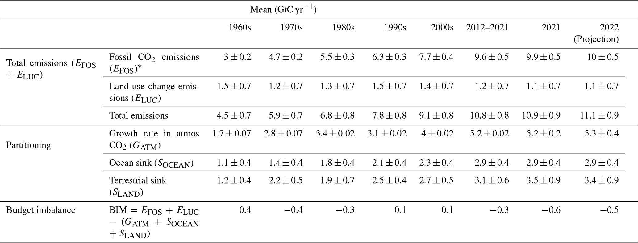
∗ Fossil emissions excluding the cement carbonation sink amount to 3.1 ± 0.2, 4.7 ± 0.2, 5.5 ± 0.3, 6.4 ± 0.3, 7.9 ± 0.4, and 9.8 ± 0.5 GtC yr−1 for the decades of the 1960s to 2010s, respectively, 10.1 ± 0.5 GtC yr−1 for 2021, and 10.2 ± 0.5 GtC yr−1 for 2022.
Table 7Comparison of the projection with realized fossil CO2 emissions (EFOS). The “actual” values are the first estimate available using actual data, and the “projected” values refer to estimates made before the end of the year for each publication. Projections based on a different method from that described here during 2008–2014 are available in Le Quéré et al. (2016). All values are adjusted for leap years.
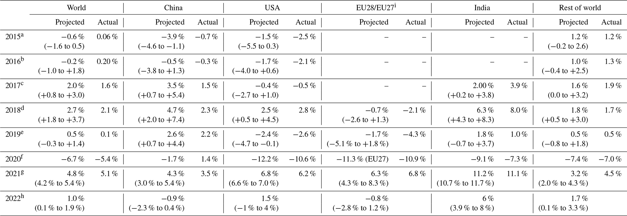
a Jackson et al. (2016) and Le Quéré et al. (2015a). b Le Quéré et al. (2016). c Le Quéré et al. (2018a). d Le Quéré et al. (2018b). e Friedlingstein et al. (2019), f Friedlingstein et al. (2020), g Friedlingstein et al. (2022a), h This study. i EU28 up to 2019 and EU27 from 2020.
Table 8Cumulative CO2 for different time periods in gigatonnes of carbon (GtC). Fossil CO2 emissions include cement carbonation. The budget imbalance (BIM) provides a measure of the discrepancies among the nearly independent estimates. All values are rounded to the nearest 5 GtC, and therefore columns do not necessarily add to zero. Uncertainties are reported as follows: EFOS is 5 % of cumulative emissions, ELUC prior to 1959 is 1σ spread from the DGVMs, ELUC post-1959 is 0.7 times the number of years (where 0.7 GtC yr−1 is the uncertainty on the annual ELUC flux estimate), GATM uncertainty is held constant at 5 GtC for all time periods, SOCEAN uncertainty is 20 % of the cumulative sink (20 % relates to the annual uncertainty of 0.4 GtC yr−1, which is ∼ 20 % of the current ocean sink), and SLAND is the 1σ spread from the DGVM estimates.
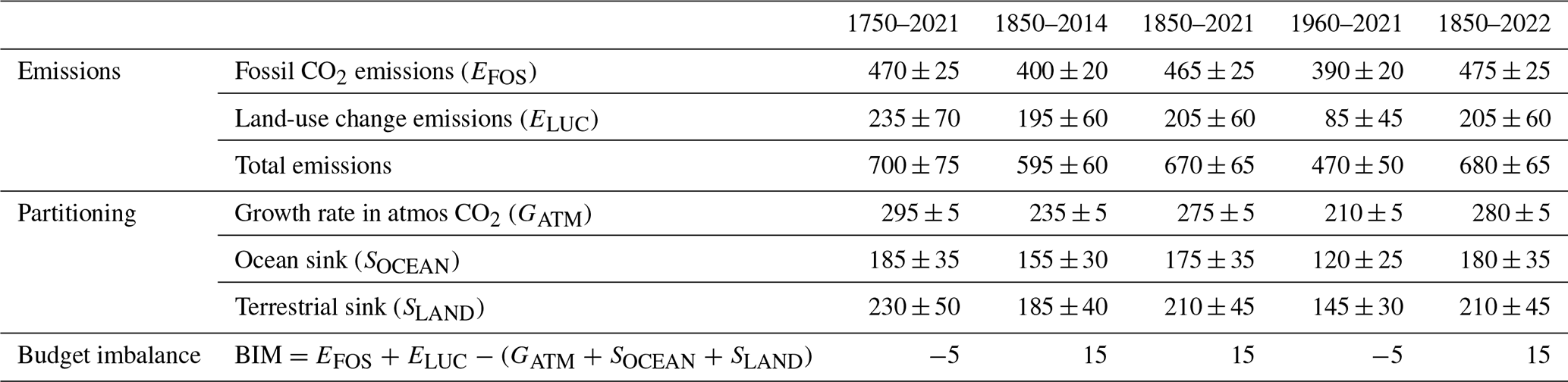
3.4 Atmospheric CO2
3.4.1 Historical period 1850–2021
Atmospheric CO2 concentration was approximately 278 ppm in 1750, 300 ppm in the 1910s, 350 ppm in the late 1980s, and 414.71 ± 0.1 ppm in 2021 (Dlugokencky and Tans, 2022); Fig. 1). The mass of carbon in the atmosphere increased by 48 % from 590 GtC in 1750 to 879 GtC in 2021. Current CO2 concentrations in the atmosphere are unprecedented in the last 2 million years, and the current rate of atmospheric CO2 increase is at least 10 times faster than at any other time during the last 800 000 years (Canadell et al., 2021).
3.4.2 Recent period 1960–2021
The growth rate in atmospheric CO2 level increased from 1.7 ± 0.07 GtC yr−1 in the 1960s to 5.2 ± 0.02 GtC yr−1 during 2012–2022 with important decadal variations (Table 6, Figs. 3 and 4). During the last decade (2012–2021), the growth rate in atmospheric CO2 concentration continued to increase, albeit with large interannual variability (Fig. 4).
The airborne fraction (AF), defined as the ratio of atmospheric CO2 growth rate to total anthropogenic emissions, i.e.
provides a diagnostic of the relative strength of the land and ocean carbon sinks in removing part of the anthropogenic CO2 perturbation. The evolution of AF over the last 60 years shows no significant trend, remaining at around 44 %, albeit showing a large interannual and decadal variability driven by the year-to-year variability in GATM (Fig. 9). The observed stability of the airborne fraction over the 1960–2020 period indicates that the ocean and land CO2 sinks have on average been removing about 55 % of the anthropogenic emissions (see Sect. 3.5 and 3.6).

Figure 8(a) The land CO2 sink (SLAND) estimated by individual DGVM estimates (green), as well as the budget estimate (black with ±1σ uncertainty), which is the average of all DGVMs. (b) Total atmosphere–land CO2 fluxes (SLAND−ELUC). The budget estimate of the total land flux (black with ± 1σ uncertainty) combines the DGVM estimate of SLAND from panel (a) with the bookkeeping estimate of ELUC from Fig. 7a. Uncertainties are similarly propagated in quadrature from the budget estimates of SLAND from panel (a) and ELUC from Fig. 7a. DGVMs also provide estimates of ELUC (see Fig. 7a), which can be combined with their own estimates of the land sink. Hence, panel (b) also includes an estimate for the total land flux for individual DGVMs (thin green lines) and their multi-model mean (thick green line).
3.4.3 Final year 2021
The growth rate in atmospheric CO2 concentration was 5.2 ± 0.2 GtC (2.46 ± 0.08 ppm) in 2021 (Fig. 4; Dlugokencky and Tans, 2022), slightly above the 2020 growth rate (5.0 GtC) but similar to the 2011–2020 average (5.2 GtC).
3.4.4 Year 2022 projection
The 2022 growth in atmospheric CO2 concentration (GATM) is projected to be about 5.3 GtC (2.5 ppm) based on global observations until October 2022, bringing the atmospheric CO2 concentration to an expected level of 417.2 ppm averaged over the year, 51 % over the preindustrial level.
3.5 Ocean sink
3.5.1 Historical period 1850–2021
Cumulated since 1850, the ocean sink adds up to 175 ± 35 GtC, with more than two-thirds of this amount (120 GtC) being taken up by the global ocean since 1960. Over the historical period, the ocean sink increased in pace with the exponential anthropogenic emissions increase (Fig. 3b). Since 1850, the ocean has removed 26 % of total anthropogenic emissions.
3.5.2 Recent period 1960–2021
The ocean CO2 sink increased from 1.1 ± 0.4 GtC yr−1 in the 1960s to 2.9 ± 0.4 GtC yr−1 during 2012–2021 (Table 6), with interannual variations of the order of a few tenths of a gigatonne of carbon per year (Fig. 10). The ocean-borne fraction () has been remarkably constant at around 25 % on average (Fig. 9). Variations around this mean illustrate decadal variability of the ocean carbon sink. So far there is no indication of a decrease in the ocean-borne fraction from 1960 to 2021. The increase in the ocean sink is primarily driven by the increased atmospheric CO2 concentration, with the strongest CO2-induced signal in the North Atlantic Ocean and the Southern Ocean (Fig. 11a). The effect of climate change is much weaker, reducing the ocean sink globally by 0.11 ± 0.09 GtC yr−1 (−4.2 %) during 2012–2021 (nine models simulate a weakening of the ocean sink by climate change with a range of −3.2 to −8.9 %, and only one model simulates a strengthening by 4.8 %), and it does not show clear spatial patterns across the GOBM ensemble (Fig. 11b). This is the combined effect of change and variability in all atmospheric forcing fields, previously attributed to wind and temperature changes in one model (Le Quéré et al., 2010).
Table 9Mapping of global carbon cycle model land flux definitions to the definition of the LULUCF net flux used in national Greenhouse Gas Inventories reported to UNFCCC. See Sect. C2.3 and Table A8 for details on the methodology and a comparison to other data sets.
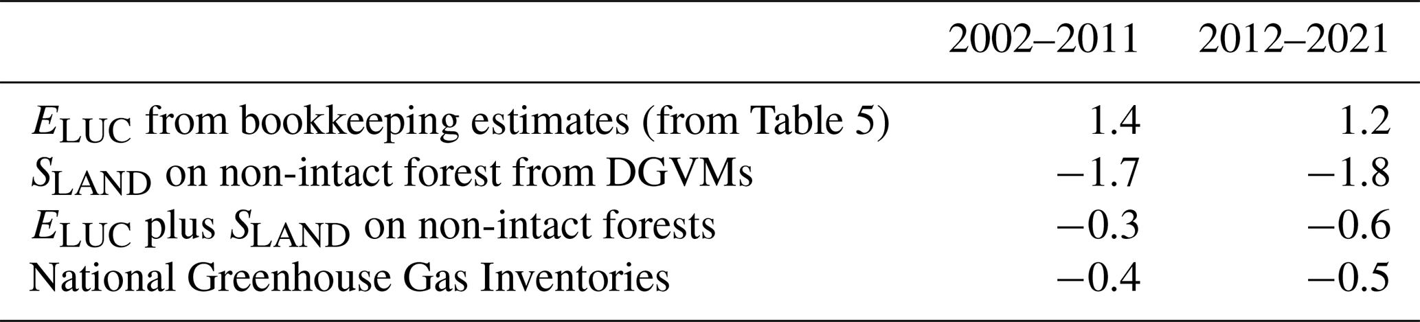
The global net air–sea CO2 flux is a residual of large natural and anthropogenic CO2 fluxes into and out of the ocean with distinct regional and seasonal variations (Figs. 6 and B1). Natural fluxes dominate on regional scales but largely cancel out when integrated globally (Gruber et al., 2009). Mid-latitudes in all basins and the high-latitude North Atlantic dominate the ocean CO2 uptake where low temperatures and high wind speeds facilitate CO2 uptake at the surface (Takahashi et al., 2009). In these regions, formation of mode, intermediate, and deep-water masses transport anthropogenic carbon into the ocean interior, thus allowing for continued CO2 uptake at the surface. Outgassing of natural CO2 occurs mostly in the tropics, especially in the equatorial upwelling region, and to a lesser extent in the North Pacific and polar Southern Ocean, mirroring a well-established understanding of regional patterns of air–sea CO2 exchange (e.g. Takahashi et al., 2009; Gruber et al., 2009). These patterns are also noticeable in the Surface Ocean CO2 Atlas (SOCAT) data set, where an ocean fCO2 value above the atmospheric level indicates outgassing (Fig. B1). This map further illustrates the data sparsity in the Indian Ocean and the Southern Hemisphere in general.
Interannual variability of the ocean carbon sink is driven by climate variability with a first-order effect from a stronger ocean sink during large El Niño events (e.g. 1997–1998) (Fig. 10; Rödenbeck et al., 2014; Hauck et al., 2020). The GOBMs show the same patterns of decadal variability as the mean of the fCO2-based data products, with a stagnation of the ocean sink in the 1990s and a strengthening since the early 2000s (Fig. 10, Le Quéré et al., 2007; Landschützer et al., 2015, 2016; DeVries et al., 2017; Hauck et al., 2020; McKinley et al., 2020). Different explanations have been proposed for this decadal variability, ranging from the ocean's response to changes in atmospheric wind and pressure systems (e.g. Le Quéré et al., 2007; Keppler and Landschützer, 2019), including variations in upper-ocean overturning circulation (DeVries et al., 2017), to the eruption of Mount Pinatubo and its effects on sea surface temperature and slowed atmospheric CO2 growth rate in the 1990s (McKinley et al., 2020). The main origin of the decadal variability is a matter of debate, with a number of studies initially pointing to the Southern Ocean (see review in Canadell et al., 2021), but contributions from the North Atlantic and North Pacific oceans (Landschützer et al., 2016; DeVries et al., 2019) or a global signal (McKinley et al., 2020) were also proposed.
Although all individual GOBMs and data products fall within the observational constraint, the ensemble means of GOBMs and data products adjusted for the riverine flux diverge over time with a mean offset increasing from 0.28 GtC yr−1 in the 1990s to 0.61 GtC yr−1 in the decade 2012–2021 and reaching 0.79 GtC yr−1 in 2021. The SOCEAN positive trend over time has diverged by a factor of 2 since 2002 (GOBMs: 0.28 ± 0.07 GtC yr−1 per decade; data products: 0.61 ± 0.17 GtC yr−1 per decade; SOCEAN: 0.45 GtC yr−1 per decade) and by a factor of 3 since 2010 (GOBMs: 0.21 ± 0.14 GtC yr−1 per decade; data products: 0.66 ± 0.38 GtC yr−1 per decade; SOCEAN: 0.44 GtC yr−1 per decade). The GOBM estimate is slightly higher (< 0.1 GtC yr−1) than in the previous global carbon budget (Friedlingstein et al., 2022a) because two new models are included (CESM2, MRI) and four models revised their estimates upwards (CESM-ETHZ, CNRM, FESOM2-REcoM, PlankTOM). The data product estimate is higher by about 0.1 GtC yr−1 compared to Friedlingstein et al. (2022a) as a result of an upward correction in three products (Jena-MLS, MPI-SOMFFN, OS-ETHZ-Gracer), the submission of LDEO-HPD (which is above average), the non-availability of the CSIR product, and the small upward correction of the river flux adjustment.
The discrepancy between the two types of estimates stems mostly from a larger Southern Ocean sink in the data products prior to 2001 and from a larger SOCEAN trend in the northern and southern extratropics since then (Fig. 13). Note that the location of the mean offset (but not its trend) depends strongly on the choice of regional river flux adjustment and would occur in the tropics rather than in the Southern Ocean when using the data set of Lacroix et al. (2020) instead of Aumont et al. (2001). Other possible explanations for the discrepancy in the Southern Ocean could be missing winter observations and data sparsity in general (Bushinsky et al., 2019, Gloege et al., 2021) or model biases (as indicated by the large model spread in the Southern Hemisphere, as shown in Fig. 13, and the larger model–data mismatch, as shown in Fig. B2).
In GCB releases until 2021, the ocean sink 1959–1989 was only estimated by GOBMs due to the absence of fCO2 observations. Now, the first data-based estimates extending back to 1957/58 are becoming available (Jena-MLS, Rödenbeck et al., 2022, LDEO-HPD, Bennington et al., 2022; Gloege et al., 2022). These are based on a multi-linear regression of pCO2 with environmental predictors (Rödenbeck et al., 2022, included here) or on model–data pCO2 misfits and their relation to environmental predictors (Bennington et al., 2022). The Jena-MLS estimate falls well within the range of GOBM estimates and has a correlation of 0.98 with SOCEAN (1959–2021 and 1959–1989). It agrees well on the mean SOCEAN estimate since 1977 with a slightly higher amplitude of variability (Fig. 10). Until 1976, Jena-MLS is 0.2–0.3 GtC yr−1 below the central SOCEAN estimate. The agreement, especially on phasing of variability, is impressive, and the discrepancies in the mean flux 1959–1976 could be explained by an overestimated trend of Jena-MLS (Rödenbeck et al., 2022). Bennington et al. (2022) report a larger flux into the pre-1990 ocean than in Jena-MLS.
The reported SOCEAN estimate from GOBMs and data products is 2.1 ± 0.4 GtC yr−1 over the period 1994 to 2007, which is in agreement with the ocean interior estimate of 2.2 ± 0.4 GtC yr−1, which accounts for the climate effect on the natural CO2 flux of −0.4 ± 0.24 GtC yr−1 (Gruber et al., 2019) to match the definition of SOCEAN used here (Hauck et al., 2020). This comparison depends critically on the estimate of the climate effect on the natural CO2 flux, which is smaller from the GOBMs (−0.1 GtC yr−1) than in Gruber et al. (2019). Uncertainties in these two estimates would also overlap when using the GOBM estimate of the climate effect on the natural CO2 flux.
During 2010–2016, the ocean CO2 sink appears to have intensified in line with the expected increase from atmospheric CO2 (McKinley et al., 2020). This effect is stronger in the fCO2-based data products (Fig. 10, ocean sink 2016 minus 2010, GOBMs: +0.42 ± 0.09 GtC yr−1; data products: +0.52 ± 0.22 GtC yr−1). The reduction of −0.09 GtC yr−1 (range: −0.39 to +0.01 GtC yr−1) in the ocean CO2 sink in 2017 is consistent with the return to normal conditions after the El Niño in 2015/16, which caused an enhanced sink in previous years. After 2017, the GOBM ensemble mean suggests the ocean sink levelling off at about 2.6 GtC yr−1, whereas the data product estimate increases by 0.24 ± 0.17 GtC yr−1 over the same period.
3.5.3 Final year 2021
The estimated ocean CO2 sink was 2.9 ± 0.4 GtC in 2021. This is a decrease of 0.12 GtC compared to 2020, in line with the expected sink weakening from persistent La Niña conditions. GOBM and data product estimates consistently result in a stagnation of SOCEAN (GOBMs: −0.09 ± 0.15 GtC; data products: −0.15 ± 0.24 GtC). Seven models and six data products show a decrease in SOCEAN (GOBMs down to −0.31 GtC, data products down to −0.58 GtC), while three models and two data products show an increase in SOCEAN (GOBMs up to 0.15 GtC, data products up to 0.12 GtC; Fig. 10). The data products have a larger uncertainty at the tails of the reconstructed time series (e.g. Watson et al., 2020). Specifically, the data products' estimate of the last year is regularly adjusted in the following release owing to the tail effect and an incrementally increasing data availability with a 1–5-year lag (Fig. 10 inset).
3.5.4 Year 2022 projection
Using a feed-forward neural network method (see Sect. 2.4) we project an ocean sink of 2.9 GtC for 2022. This is similar to the year 2021 as the La Niña conditions persist in 2022.
3.5.5 Model evaluation
The additional simulation D allows us to separate the anthropogenic carbon component (steady state and non-steady state, sim D − sim A) and compare the model flux and dissolved inorganic carbon (DIC) inventory change directly to the interior ocean estimate of Gruber et al. (2019) without further assumptions. The GOBM ensemble average of anthropogenic carbon inventory changes 1994–2007 amounts to 2.2 GtC yr−1 and is thus lower than the 2.6 ± 0.3 GtC yr−1 estimated by Gruber et al. (2019). Only four models with the highest sink estimate fall within the range reported by Gruber et al. (2019). This suggests that the majority of the GOBMs underestimate anthropogenic carbon uptake by 10 %–20 %. Analysis of Earth system models indicate that an underestimation by about 10 % may be due to biases in ocean carbon transport and mixing from the surface mixed layer to the ocean interior (Goris et al., 2018; Terhaar et al., 2021; Bourgeois et al., 2022; Terhaar et al., 2022), biases in the chemical buffer capacity (Revelle factor) of the ocean (Vaittinada Ayar et al., 2022; Terhaar et al., 2022), and partly due to the late starting date of the simulations (mirrored in atmospheric CO2 chosen for the pre-industrial control simulation, Table A2, Bronselaer et al., 2017; Terhaar et al., 2022). Interestingly, and in contrast to the uncertainties in the surface CO2 flux, we find the largest mismatch in interior ocean carbon accumulation in the tropics (93 % of the mismatch), with minor contribution from the north (1 %) and the south (6 %). This highlights the role of interior ocean carbon redistribution for those inventories (Khatiwala et al., 2009).

Figure 9The partitioning of total anthropogenic CO2 emissions (EFOS+ELUC) across (a) the atmosphere (airborne fraction), (b) land (land-borne fraction), and (c) ocean (ocean-borne fraction). Black lines represent the central estimate, and the coloured shading represents the uncertainty. The dashed grey lines represent the long-term average of the airborne (44 %), land-borne (30 %), and ocean-borne (25 %) fractions during 1960–2021.
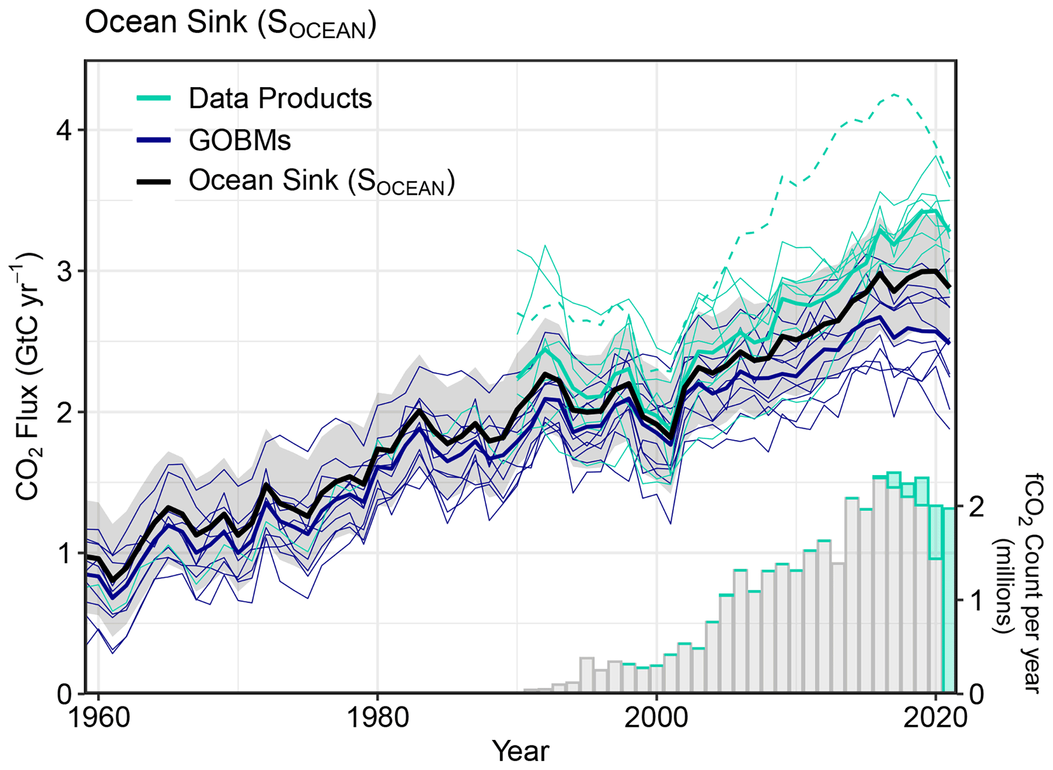
Figure 10Comparison of the anthropogenic atmosphere–ocean CO2 flux showing the budget values of SOCEAN (black; with the uncertainty in grey shading), individual ocean models (royal blue), and the ocean fCO2-based data products (cyan; with Watson et al. , 2020, shown as a dashed line as it is not used for the ensemble mean). Only one data product (Jena-MLS) extends back to 1959 (Rödenbeck et al., 2022). The fCO2-based data products were adjusted for the pre-industrial ocean source of CO2 from river input to the ocean by subtracting a source of 0.65 GtC yr−1 to make them comparable to SOCEAN (see Sect. 2.4). The bar plot in the lower right illustrates the number of fCO2 observations in the SOCAT v2022 database (Bakker et al., 2022). Grey bars indicate the number of data points in SOCAT v2021, and coloured bars show the newly added observations in v2022.
The evaluation of the ocean estimates (Fig. B2) shows a root-mean-squared error (RMSE) from annually detrended data of 0.4 to 2.6 µatm for the seven fCO2-based data products over the globe, relative to the fCO2 observations from the SOCAT v2022 data set for the period 1990–2021. The GOBM RMSEs are larger and range from 3.0 to 4.8 µatm. The RMSEs are generally larger at high latitudes compared to the tropics, for both the data products and the GOBMs. The data products have RMSEs of 0.4 to 3.2 µatm in the tropics, 0.8 to 2.8 µatm in the northern extratropics (> 30∘ N), and 0.8 to 3.6 µatm in the southern extratropics (< 30∘ S). Note that the data products are based on the SOCAT v2022 database; hence, the SOCAT is not an independent data set for the evaluation of the data products. The GOBM RMSEs are more spread across regions, ranging from 2.5 to 3.9 µatm in the tropics, 3.1 to 6.5 µatm in the north, and 5.4 to 7.9 µatm in the south. The higher RMSEs occur in regions with stronger climate variability, such as the northern and southern high latitudes (poleward of the subtropical gyres). The upper ranges of the model RMSEs have decreased somewhat relative to Friedlingstein et al. (2022a).
3.6 Land sink
3.6.1 Historical period 1850–2021
Cumulated since 1850, the terrestrial CO2 sink amounts to 210 ± 45 GtC, 31 % of total anthropogenic emissions. Over the historical period, the sink increased in pace with the exponential anthropogenic emissions increase (Fig. 3b).
3.6.2 Recent period 1960–2021
The terrestrial CO2 sink increased from 1.2 ± 0.4 GtC yr−1 in the 1960s to 3.1 ± 0.6 GtC yr−1 during 2012–2021, with important interannual variations of up to 2 GtC yr−1 generally showing a decreased land sink during El Niño events (Fig. 8), responsible for the corresponding enhanced growth rate in atmospheric CO2 concentration. The larger land CO2 sink during 2012–2021 compared to the 1960s is reproduced by all the DGVMs in response to the increase in both atmospheric CO2 and nitrogen deposition and the changes in climate and is consistent with constraints from the other budget terms (Table 5).
Over the period 1960 to present the increase in the global terrestrial CO2 sink is largely attributed to the CO2 fertilization effect (Prentice et al., 2001; Piao et al., 2009), directly stimulating plant photosynthesis and increased plant water use in water-limited systems, with a small negative contribution of climate change (Fig. 11). There is a range of evidence to support a positive terrestrial carbon sink in response to increasing atmospheric CO2, albeit with uncertain magnitude (Walker et al., 2021). As expected from theory, the greatest CO2 effect is simulated in the tropical forest regions, associated with warm temperatures and long growing seasons (Hickler et al., 2008) (Fig. 11a). However, evidence from tropical intact forest plots indicate an overall decline in the land sink across Amazonia (1985–2011), attributed to enhanced mortality offsetting productivity gains (Brienen et al., 2005, Hubau et al., 2020). During 2012–2021 the land sink is positive in all regions (Fig. 6) with the exception of eastern Brazil, the southwestern US, southeastern Europe, central Asia, northern and southern Africa, and eastern Australia, where the negative effects of climate variability and change (i.e. reduced rainfall) counterbalance CO2 effects. This is clearly visible in Fig. 11 where the effects of CO2 (Fig. 11a) and climate (Fig. 11b) as simulated by the DGVMs are isolated. The negative effect of climate is the strongest in most of South America, Central America, the southwestern US, central Europe, western Sahel, southern Africa, Southeast Asia and southern China, and eastern Australia (Fig. 11b). Globally, climate change reduces the land sink by 0.63 ± 0.52 GtC yr−1 or 17 % (2012–2021).
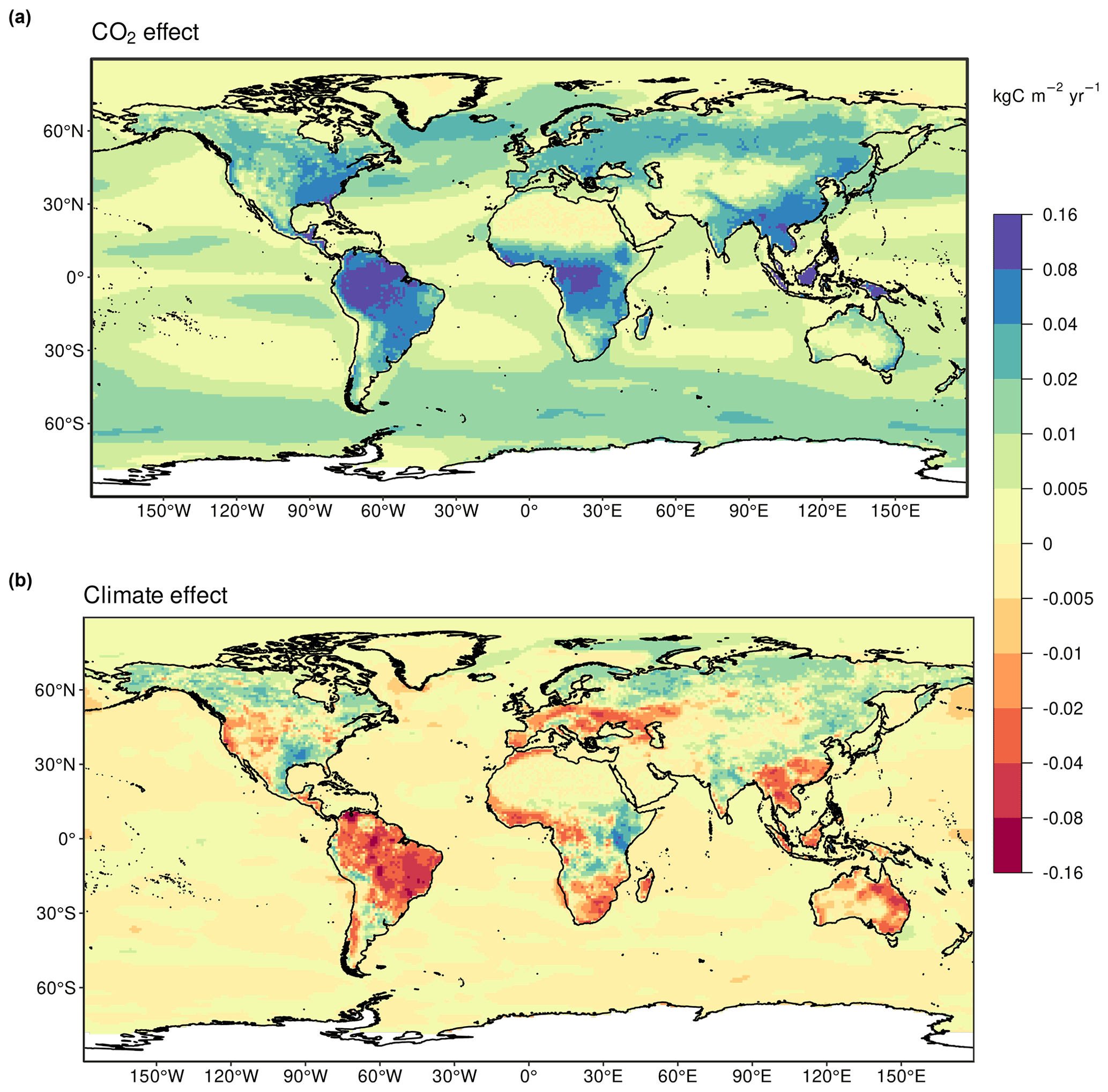
Figure 11Attribution of the atmosphere–ocean (SOCEAN) and atmosphere–land (SLAND) CO2 fluxes to (a) increasing atmospheric CO2 concentrations and (b) changes in climate, averaged over the previous decade 2012–2021. All data shown are from the processed-based GOBMs and DGVMs. The sum of ocean CO2 and climate effects will not equal the ocean sink shown in Fig. 6, which includes the fCO2-based data products. See Appendices C3.2 and C4.1 for attribution methodology. Units are in kgC m−2 yr−1 (note the non-linear colour scale).
Since 2020 the globe has experienced La Niña conditions, which would be expected to lead to an increased land carbon sink. A clear peak in the global land sink is not evident in SLAND, and we find that a La Niña-driven increase in tropical land sink is offset by a reduced high latitude extratropical land sink, which may be linked to the land response to recent climate extremes. In the past years several regions experienced record-setting fire events. While global burned area has declined over the past decades, mostly due to declining fire activity in savannas (Andela et al., 2017), forest fire emissions are rising and have the potential to counter the negative fire trend in savannas (Zheng et al., 2021). Noteworthy events include the Black Summer event in Australia in 2019–2020 (emissions of roughly 0.2 GtC; van der Velde et al., 2021) and events in Siberia in 2021 where emissions approached 0.4 GtC or 3 times the 1997–2020 average according to GFED4s. While other regions, including the western US and Mediterranean Europe, also experienced intense fire seasons in 2021, their emissions are substantially lower.
Despite these regional negative effects of climate change on SLAND, the efficiency of land to remove anthropogenic CO2 emissions has remained broadly constant over the last 6 decades, with a land-borne fraction ()) of ∼ 30 % (Fig. 9).
3.6.3 Final year 2021
The terrestrial CO2 sink from the DGVMs ensemble was 3.5 ± 0.9 GtC in 2021, slightly above the decadal average of 3.1 ± 0.6 GtC yr−1 (Fig. 4, Table 6). We note that the DGVM estimate for 2021 is larger than, but within the uncertainty of, the 2.8 ± 0.9 GtC yr−1 estimate from the residual sink from the global budget () (Table 5).
3.6.4 Year 2022 projection
Using a feed-forward neural network method we project a land sink of 3.4 GtC for 2022, very similar to the 2021 estimate. As for the ocean sink, we attribute this to the persistence of La Niña conditions in 2022.
3.6.5 Model evaluation
The evaluation of the DGVMs (Fig. B3) shows generally high skill scores across models for runoff and to a lesser extent for vegetation biomass, gross primary production (or productivity; GPP), and ecosystem respiration (Fig. B3, left panel). Skill score was lowest for leaf area index and net ecosystem exchange, with the widest disparity among models for soil carbon. These conclusions are supported by a more comprehensive analysis of DGVM performance in comparison with benchmark data (Seiler et al., 2022). Furthermore, results show how DGVM differences are often of similar magnitude compared with the range across observational data sets.
3.7 Partitioning the carbon sinks
3.7.1 Global sinks and spread of estimates
In the period 2012–2021, the bottom-up view of total global carbon sinks provided by the GCB, SOCEAN for the ocean and SLAND–ELUC for the land (to be comparable to inversions), agrees closely with the top-down global carbon sinks delivered by the atmospheric inversions. Figure 12 shows both total sink estimates of the last decade split by ocean and land (including ELUC), which match the difference between GATM and EFOS to within 0.01–0.12 GtC yr−1 for inverse systems, and to 0.34 GtC yr−1 for the GCB mean. The latter represents the BIM discussed in Sect. 3.8, which by design is minimal for the inverse systems.

Figure 12The 2012–2021 decadal mean net atmosphere–ocean and atmosphere–land fluxes derived from the ocean models and fCO2 products (y axis, right- and left-pointing blue triangles, respectively) and from the DGVMs (x axis, green symbols) and the same fluxes estimated from the inversions (purple symbols on secondary x and y axes). The grey central point is the mean (±1σ) of SOCEAN and (SLAND−ELUC) as assessed in this budget. The shaded distributions show the density of the ensemble of individual estimates. The grey diagonal band represents the fossil fuel emissions minus the atmospheric growth rate from this budget (). Note that positive values are CO2 sinks.
The distributions based on the individual models and data products reveal substantial spread but converge near the decadal means quoted in Tables 5 and 6. Sink estimates for SOCEAN and from inverse systems are mostly non-Gaussian, while the ensemble of DGVMs appears more normally distributed, justifying the use of a multi-model mean and standard deviation for their errors in the budget. Noteworthy is that the tails of the distributions provided by the land and ocean bottom-up estimates would not agree with the global constraint provided by the fossil fuel emissions and the observed atmospheric CO2 growth rate (EFOS−GATM). This illustrates the power of the atmospheric joint constraint from GATM and the global CO2 observation network it derives from.
3.7.2 Total atmosphere-to-land fluxes
The total atmosphere-to-land fluxes (SLAND−ELUC), calculated here as the difference between SLAND from the DGVMs and ELUC from the bookkeeping models, amounts to a 1.9 ± 0.9 GtC yr−1 sink during 2012–2021 (Table 5). Estimates of total atmosphere-to-land fluxes (SLAND−ELUC) from the DGVMs alone (1.5 ± 0.5 GtC yr−1) are consistent with this estimate and also with the global carbon budget constraint (, 1.5 ± 0.6 GtC yr−1 Table 5). For the last decade (2012–2021), the inversions estimate the net atmosphere-to-land uptake to lie within a range of 1.1 to 1.7 GtC yr−1, consistent with the GCB and DGVM estimates of SLAND−ELUC (Fig. 13 top row).
3.7.3 Total atmosphere-to-ocean fluxes
For the 2012–2021 period, the GOBMs (2.6 ± 0.5 GtC yr−1) produce a lower estimate for the ocean sink than the fCO2-based data products (3.2 ± 0.6 GtC yr−1), which shows up in Fig. 12 as a separate peak in the distribution from the GOBMs (triangle symbols pointing right) and from the fCO2-based products (triangle symbols pointing left). Atmospheric inversions (2.7 to 3.3 GtC yr−1) also suggest higher ocean uptake in the last decade (Fig. 13 top row). In interpreting these differences, we caution that the riverine transport of carbon taken up on land and outgassing from the ocean is a substantial (0.65 GtC yr−1) and uncertain term that separates the various methods. A recent estimate of decadal ocean uptake from observed ratios (Tohjima et al., 2019) also points towards a larger ocean sink, albeit with large uncertainty (2012–2016: 3.1 ± 1.5 GtC yr−1).
3.7.4 Regional breakdown and interannual variability
Figure 13 also shows the latitudinal partitioning of the total atmosphere-to-surface fluxes excluding fossil CO2 emissions () according to the multi-model average estimates from GOBMs and ocean fCO2-based products (SOCEAN) and DGVMs (SLAND−ELUC) and from atmospheric inversions (SOCEAN and SLAND−ELUC).
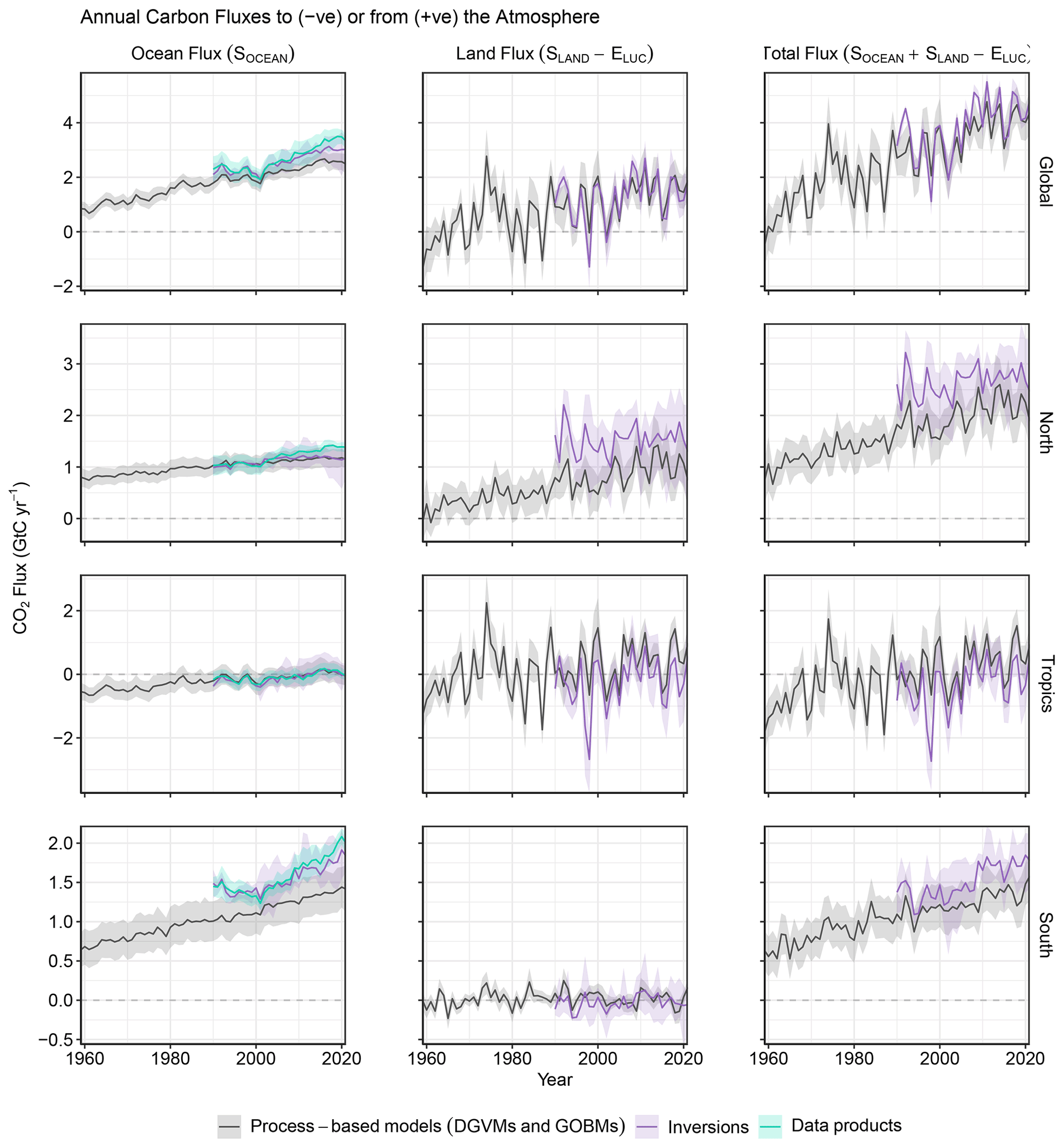
Figure 13CO2 fluxes between the atmosphere and the Earth's surface separated between land and oceans globally and in three latitude bands. The ocean flux is SOCEAN, and the land flux is the net of atmosphere–land fluxes from the DGVMs. The latitude bands are (top row) global, (second row) north (> 30∘ N), (third row) tropics (30∘ S–30∘ N), and (bottom row) south (< 30∘ S), showing values over ocean (left column) and land (middle column) and in total (right column). Estimates are shown for process-based models (DGVMs for land, GOBMs for oceans), inversion systems (land and ocean), and fCO2-based data products (ocean only). Positive values indicate a flux from the atmosphere to the land or the ocean. Mean estimates from the combination of the process models for the land and oceans are shown (black line) with ±1 standard deviation (1σ) of the model ensemble (grey shading). For the total uncertainty in the process-based estimate of the total sink, uncertainties are summed in quadrature. Mean estimates from the atmospheric inversions are shown (purple lines) with their full spread (purple shading). Mean estimates from the fCO2-based data products are shown for the ocean domain (light blue lines) with their ±1σ spread (light blue shading). The global SOCEAN (upper left) and the sum of SOCEAN in all three regions represents the anthropogenic atmosphere-to-ocean flux based on the assumption that the pre-industrial ocean sink was 0 GtC yr−1 when riverine fluxes are not considered. This assumption does not hold at the regional level, where pre-industrial fluxes can be significantly different from zero. Hence, the regional panels for SOCEAN represent a combination of natural and anthropogenic fluxes. Bias correction and area weighting were only applied to global SOCEAN; hence, the sum of the regions is slightly different from the global estimate (< 0.05 GtC yr−1).
North
Despite being one of the most densely observed and studied regions of our globe, annual mean carbon sink estimates in the northern extratropics (north of 30∘ N) continue to differ. The atmospheric inversions suggest an atmosphere-to-surface sink () for 2012–2021 of 2.0 to 3.2 GtC yr−1, which is higher than the process models' estimate of 2.2 ± 0.4 GtC yr−1 (Fig. 13). The GOBMs (1.2 ± 0.2 GtC yr−1), fCO2-based data products (1.4 ± 0.1 GtC yr−1), and inversion systems (0.9 to 1.4 GtC yr−1) produce consistent estimates of the ocean sink. Thus, the difference mainly arises from the total land flux (SLAND−ELUC) estimate, which is 1.0 ± 0.4 GtC yr−1 in the DGVMs compared to 0.6 to 2.0 GtC yr−1 in the atmospheric inversions (Fig. 13, second row).
Discrepancies in the northern land fluxes conform with persistent issues surrounding the quantification of the drivers of the global net land CO2 flux (Arneth et al., 2017; Huntzinger et al., 2017; O'Sullivan et al., 2022) and the distribution of atmosphere-to-land fluxes between the tropics and high northern latitudes (Baccini et al., 2017; Schimel et al., 2015; Stephens et al., 2007; Ciais et al., 2019; Gaubert et al., 2019).
In the northern extratropics, the process models, inversions, and fCO2-based data products consistently suggest that most of the variability stems from the land (Fig. 13). Inversions generally estimate similar interannual variations (IAVs) over land to DGVMs (0.30–0.37 vs. 0.17–0.69 GtC yr−1, averaged over 1990–2021), and they have higher IAV in ocean fluxes (0.05–0.09 GtC yr−1) relative to GOBMs (0.02–0.06 GtC yr−1, Fig. B2) and fCO2-based data products (0.03–0.09 GtC yr−1).
Tropics
In the tropics (30∘ S–30∘ N), both the atmospheric inversions and process models estimate a total carbon balance () that is close to neutral over the past decade. The GOBMs (0.06 ± 0.34 GtC yr−1), fCO2-based data products (0.00 ± 0.06 GtC yr−1), and inversion systems (−0.2 to 0.5 GtC yr−1) all indicate an approximately neutral tropical ocean flux (see Fig. B1 for spatial patterns). DGVMs indicate a net land sink (SLAND−ELUC) of 0.5 ± 0.3 GtC yr−1, whereas the inversion systems indicate a net land flux between −0.9 and 0.7 GtC yr−1, albeit with high uncertainty (Fig. 13, third row).
The tropical lands are the origin of most of the atmospheric CO2 interannual variability (Ahlström et al., 2015), and this is consistent among the process models and inversions (Fig. 13). The interannual variability in the tropics is similar among the ocean data products (0.07–0.16 GtC yr−1) and the GOBMs (0.07–0.16 GtC yr−1, Fig. B2), which is the highest ocean sink variability of all regions. The DGVMs and inversions indicate that atmosphere-to-land CO2 fluxes are more variable than atmosphere-to-ocean CO2 fluxes in the tropics, with interannual variability of 0.5 to 1.1 and 0.8 to 1.0 GtC yr−1 for DGVMs and inversions, respectively.
South
In the southern extratropics (south of 30∘ S), the atmospheric inversions suggest a total atmosphere-to-surface sink () for 2012–2021 of 1.6 to 1.9 GtC yr−1, slightly higher than the process models' estimate of 1.4 ± 0.3 GtC yr−1 (Fig. 13). An approximately neutral total land flux (SLAND−ELUC) for the southern extratropics is estimated by both the DGVMs (0.02 ± 0.06 GtC yr−1) and the inversion systems (sink of −0.2 to 0.2 GtC yr−1). This means nearly all carbon uptake is due to oceanic sinks south of 30∘ S. The Southern Ocean flux in the fCO2-based data products (1.8 ± 0.1 GtC yr−1) and inversion estimates (1.6 to 1.9 GtC yr−1) is higher than in the GOBMs (1.4 ± 0.3 GtC yr−1) (Fig. 13, bottom row). This discrepancy in the mean flux is likely explained by the uncertainty in the regional distribution of the river flux adjustment (Aumont et al., 2001; Lacroix et al., 2020) applied to fCO2-based data products and inverse systems to isolate the anthropogenic SOCEAN flux. Other possibly contributing factors are that the data products potentially underestimate the winter CO2 outgassing south of the Polar Front (Bushinsky et al., 2019) and potential model biases. CO2 fluxes from this region are more sparsely sampled by all methods, especially in wintertime (Fig. B1). Dominant biases in Earth system models are related to mode water formation, stratification, and the chemical buffer capacity (Terhaar et al., 2021; Bourgeois et al., 2022; Terhaar et al., 2022).
The interannual variability in the southern extratropics is low because of the dominance of ocean areas with low variability compared to land areas. The split between land (SLAND−ELUC) and ocean (SOCEAN) shows a substantial contribution to variability in the south coming from the land, with no consistency between the DGVMs and the inversions or among inversions. This is expected due to the difficulty of exactly separating the land and oceanic fluxes when viewed from atmospheric observations alone. The SOCEAN interannual variability was found to be higher in the fCO2-based data products (0.09 to 0.19 GtC yr−1) compared to GOBMs (0.03 to 0.06 GtC yr−1) in 1990–2021 (Fig. B2). Model subsampling experiments recently illustrated that observation-based products may overestimate decadal variability in the Southern Ocean carbon sink by 30 % due to data sparsity, based on one data product with the highest decadal variability (Gloege et al., 2021).
Tropical vs. northern land uptake
A continuing conundrum is the partitioning of the global atmosphere–land flux between the Northern Hemisphere land and the tropical land (Stephens et al., 2017; Pan et al., 2011; Gaubert et al., 2019). It is of importance because each region has its own history of land-use change, climate drivers, and the impact of increasing atmospheric CO2 and nitrogen deposition. Quantifying the magnitude of each sink is a prerequisite to understanding how each individual driver impacts the tropical and mid- and high-latitude carbon balance.
We define the north–south (N–S) difference as net atmosphere–land flux north of 30∘ N minus the net atmosphere–land flux south of 30∘ N. For the inversions, the N–S difference ranges from 0.1 to 2.9 GtC yr−1 across this year's inversion ensemble with a preference across models for either a smaller northern land sink with a near-neutral tropical land flux (medium N–S difference) or a large northern land sink and a tropical land source (large N–S difference).
In the ensemble of DGVMs the N–S difference is 0.6 ± 0.5 GtC yr−1, a much narrower range than the one from inversions. Only two DGVMs have a N–S difference larger than 1.0 GtC yr−1. The larger agreement across DGVMs than across inversions is to be expected as there is no correlation between northern and tropical land sinks in the DGVMs, as opposed to the inversions where the sum of the two regions being well-constrained leads to an anti-correlation between these two regions. The much smaller spread in the N–S difference between the DGVMs could help to scrutinize the inverse systems further. For example, a large northern land sink and a tropical land source in an inversion would suggest a large sensitivity to CO2 fertilization (the dominant factor driving the land sinks) for northern ecosystems, which would be not mirrored by tropical ecosystems. Such a combination could be hard to reconcile with the process understanding gained from the DGVM ensembles and independent measurements (e.g. free-air CO2 enrichment experiments). Such investigations will be further pursued in the upcoming assessment from REgional Carbon Cycle Assessment and Processes (RECCAP2; Ciais et al., 2022).
3.8 Closing the global carbon cycle
3.8.1 Partitioning of cumulative emissions and sink fluxes
The global carbon budget over the historical period (1850–2021) is shown in Fig. 3.
Emissions during the period 1850–2021 amounted to 670 ± 65 GtC and were partitioned among the atmosphere (275 ± 5 GtC; 41 %), ocean (175 ± 35 GtC; 26 %), and land (210 ± 45 GtC; 31 %). The cumulative land sink is almost equal to the cumulative land-use emissions (200 ± 60 GtC), making the global land nearly neutral over the whole 1850–2021 period.
The use of nearly independent estimates for the individual terms of the global carbon budget shows a cumulative budget imbalance of 15 GtC (2 % of total emissions) during 1850–2021 (Fig. 3, Table 8), which, if correct, suggests that emissions could be slightly too high by the same proportion (2 %) or that the combined land and ocean sinks are slightly underestimated (by about 3 %), although these are well within the uncertainty range of each component of the budget. Nevertheless, part of the imbalance could originate from the estimation of significant increase in EFOS and ELUC between the mid-1920s and the mid-1960s that is unmatched by a similar growth in atmospheric CO2 concentration as recorded in ice cores (Fig. 3). However, the known loss of additional sink capacity of 30–40 GtC (over the 1850–2020 period) due to reduced forest cover has not been accounted for in our method and would exacerbate the budget imbalance (see Appendix D4).
For the more recent 1960–2021 period where direct atmospheric CO2 measurements are available, total emissions (EFOS+ELUC) amounted to 470 ± 50 GtC, of which 390 ± 20 GtC (82 %) were caused by fossil CO2 emissions and 85 ± 45 GtC (18 %) by land-use change (Table 8). The total emissions were partitioned among the atmosphere (210 ± 5 GtC; 45 %), ocean (120 ± 25 GtC; 26 %), and land (145 ± 30 GtC; 30 %), with a near-zero (−5 GtC) unattributed budget imbalance. All components except land-use change emissions have significantly grown since 1960, with important interannual variability in the growth rate in atmospheric CO2 concentration and in the land CO2 sink (Fig. 4) and some decadal variability in all terms (Table 6). Differences with previous budget releases are documented in Fig. B5.
The global carbon budget averaged over the last decade (2012–2021) is shown in Figs. 2 and 14 (right panel) and Table 6. For this period, 89 % of the total emissions (EFOS+ELUC) were from fossil CO2 emissions (EFOS), and 11 % were from land-use change (ELUC). The total emissions were partitioned among the atmosphere (48 %), ocean (26 %), and land (29 %), with a near-zero unattributed budget imbalance (∼ 3 %). For single years, the budget imbalance can be larger (Fig. 4). For 2021, the combination of our estimated sources (10.9 ± 0.9 GtC yr−1) and sinks (11.6 ± 1.0 GtC yr−1) leads to a BIM of −0.6 GtC, suggesting a slight underestimation of the anthropogenic sources and/or an overestimation of the combined land and ocean sinks.
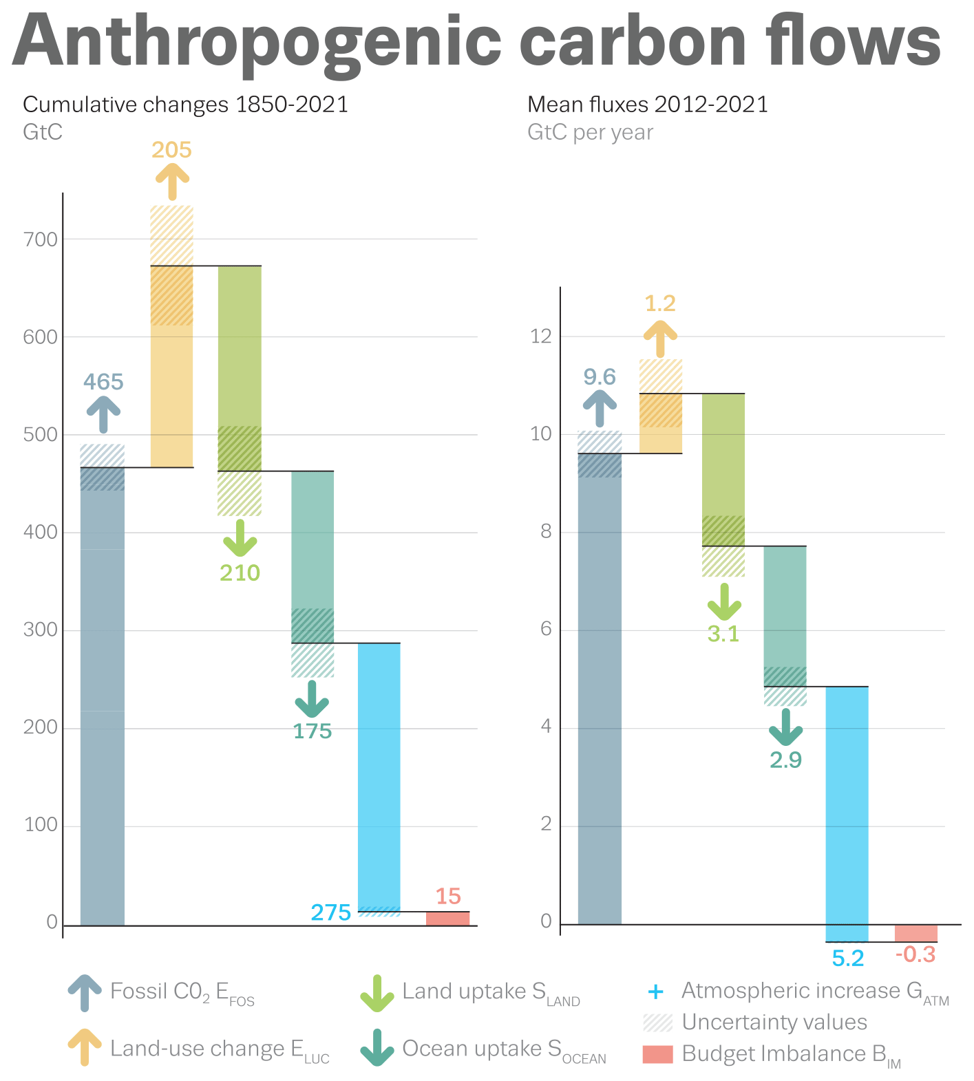
Figure 14Cumulative changes over the 1850–2021 period (left) and average fluxes over the 2012–2021 period (right) for the anthropogenic perturbation of the global carbon cycle. See the caption of Fig. 3 for key information and Sect. 2 for full details.
3.8.2 Carbon budget imbalance trend and variability
The carbon budget imbalance (BIM; Eq. 1, Fig. 4) quantifies the mismatch between the estimated total emissions and the estimated changes in the atmosphere, land, and ocean reservoirs. The mean budget imbalance from 1960 to 2021 is very small (4.6 GtC over the period, i.e. average of 0.07 GtC yr−1) and shows no trend over the full time series (Fig. 4). The process models (GOBMs and DGVMs) and data products have been selected to match observational constraints in the 1990s, but no further constraints have been applied to their representation of trend and variability. Therefore, the near-zero mean and trend in the budget imbalance is seen as evidence of a coherent community understanding of the emissions and their partitioning on those timescales (Fig. 4). However, the budget imbalance shows substantial variability on the order of ±1 GtC yr−1, particularly over semi-decadal timescales, although most of the variability is within the uncertainty of the estimates. The positive carbon imbalance during the 1960s and early 1990s indicates that either the emissions were overestimated or the sinks were underestimated during these periods. The reverse is true for the 1970s and to a lesser extent for the 1980s and the 2012–2021 period (Fig. 4, Table 6).
We cannot attribute the cause of the variability in the budget imbalance with our analysis, we only note that the budget imbalance is unlikely to be explained by errors or biases in the emissions alone because of its large semi-decadal variability component, a variability that is untypical of emissions and which has not changed in the past 60 years despite a near tripling of emissions (Fig. 4). Errors in SLAND and SOCEAN are more likely to be the main cause for the budget imbalance, especially on interannual to semi-decadal timescales. For example, underestimation of the SLAND by DGVMs has been reported following the eruption of Mount Pinatubo in 1991, possibly due to missing responses to changes in diffuse radiation (Mercado et al., 2009). Although since GCB2021 we accounted for aerosol effects on solar radiation quantity and quality (diffuse vs. direct), most DGVMs only used the former as input (i.e. total solar radiation) (Table A1). Thus, the ensemble mean may not capture the full effects of volcanic eruptions, i.e. associated with high light-scattering sulfate aerosols, on the land carbon sink (O'Sullivan et al., 2021). DGVMs are suspected to overestimate the land sink in response to the wet decade of the 1970s (Sitch et al., 2008). Quasi-decadal variability in the ocean sink has also been reported, with all methods agreeing on a smaller than expected ocean CO2 sink in the 1990s and a larger than expected sink in the 2000s (Fig. 10; Landschützer et al., 2016; DeVries et al., 2019; Hauck et al., 2020; McKinley et al., 2020). Errors in sink estimates could also be driven by errors in the climatic forcing data, particularly precipitation for SLAND and wind for SOCEAN. Also, the BIM shows substantial departure from zero on yearly timescales (Fig. 4e), highlighting unresolved variability of the carbon cycle, likely in the land sink (SLAND), given its large year-to-year variability (Figs. 4d and 8).
Both the budget imbalance (BIM, Table 6) and the residual land sink from the global budget (, Table 5) include an error term due to the inconsistencies that arise from using ELUC from bookkeeping models and SLAND from DGVMs, most notably the loss of additional sink capacity (see Sect. 2.7 and Appendix D4). Other differences include a better accounting of land-use change practices and processes in bookkeeping models than in DGVMs or the error in bookkeeping models of having present-day observed carbon densities fixed in the past. That the budget imbalance shows no clear trend towards larger values over time is an indication that these inconsistencies probably play a minor role compared to other errors in SLAND or SOCEAN.
Although the budget imbalance is near zero for the recent decades, it could be due to compensation of errors. We cannot exclude an overestimation of CO2 emissions, particularly from land-use change, given their large uncertainty, as has been suggested elsewhere (Piao et al., 2018), combined with an underestimate of the sinks. A larger DGVM (SLAND−ELUC) over the extratropics would reconcile model results with inversion estimates for fluxes in the total land during the past decade (Fig. 13; Table 5). Likewise, a larger SOCEAN is also possible given the higher estimates from the data products (see Sect. 3.1.2, Figs. 10 and 13), the underestimation of interior ocean anthropogenic carbon accumulation in the GOBMs (Sect. 3.5.5), and the recently suggested upward adjustments of the ocean carbon sink in Earth system models (Terhaar et al., 2022) and in data products, here related to a potential temperature bias and skin effects (Watson et al., 2020; Dong et al., 2022, Fig. 10). If SOCEAN were to be based on data products alone, with all data products including this adjustment, this would result in a 2012–2021 SOCEAN of 3.8 GtC yr−1 (Dong et al., 2022) or > 4 GtC yr−1 (Watson et al., 2020), i.e. outside of the range supported by the atmospheric inversions and with an implied negative BIM of more than −1 GtC yr−1, indicating that a closure of the budget could only be achieved with either anthropogenic emissions being significantly larger and/or the net land sink being substantially smaller than estimated here. More integrated use of observations in the global carbon budget, either on their own or for further constraining model results, should help resolve some of the budget imbalance (Peters et al., 2017).
The average growth in global fossil CO2 emissions peaked at +3 % per year during the 2000s, driven by the rapid growth in emissions in China. In the last decade, however, the global growth rate has slowly declined, reaching a low +0.5 % per year over 2012–2021 (including the 2020 global decline and the 2021 emissions rebound). While this slowdown in global fossil CO2 emissions growth is welcome, it is far from the emission decrease needed to be consistent with the temperature goals of the Paris Agreement.
Since the 1990s, the average growth rate of fossil CO2 emissions has continuously declined across the group of developed countries of the Organization for Economic Co-operation and Development (OECD), with emissions peaking in around 2005 and now declining at around 1 % per year (Le Quéré et al., 2021). In the decade 2012–2021, territorial fossil CO2 emissions decreased significantly (at the 95 % confidence level) in 24 countries whose economies grew significantly (also at the 95 % confidence level): Belgium, Croatia, Czech Republic, Denmark, Estonia, Finland, France, Germany, Hong Kong, Israel, Italy, Japan, Luxembourg, Malta, Mexico, Netherlands, Norway, Singapore, Slovenia, Sweden, Switzerland, the United Kingdom, the USA, and Uruguay (updated from Le Quéré et al., 2019). Altogether, these 24 countries emitted 2.4 GtC yr−1 (8.8 GtCO2 yr−1) on average over the last decade, about a quarter of world fossil CO2 emissions. Consumption-based emissions also fell significantly during the final decade for which estimates are available (2011–2020) in 15 of these countries: Belgium, Denmark, Estonia, Finland, France, Germany, Hong Kong, Israel, Japan, Luxembourg, Mexico, Netherlands, Singapore, Sweden, the United Kingdom, and Uruguay. Figure 15 shows that the emission declines in the USA and the EU27 are primarily driven by increased decarbonization (CO2 emissions per unit energy) in the last decade compared to the previous, with smaller contributions in the EU27 from slightly weaker economic growth and slightly larger declines in energy per GDP. These countries have stable or declining energy use and thus decarbonization policies replace existing fossil fuel infrastructure (Le Quéré et al., 2019).
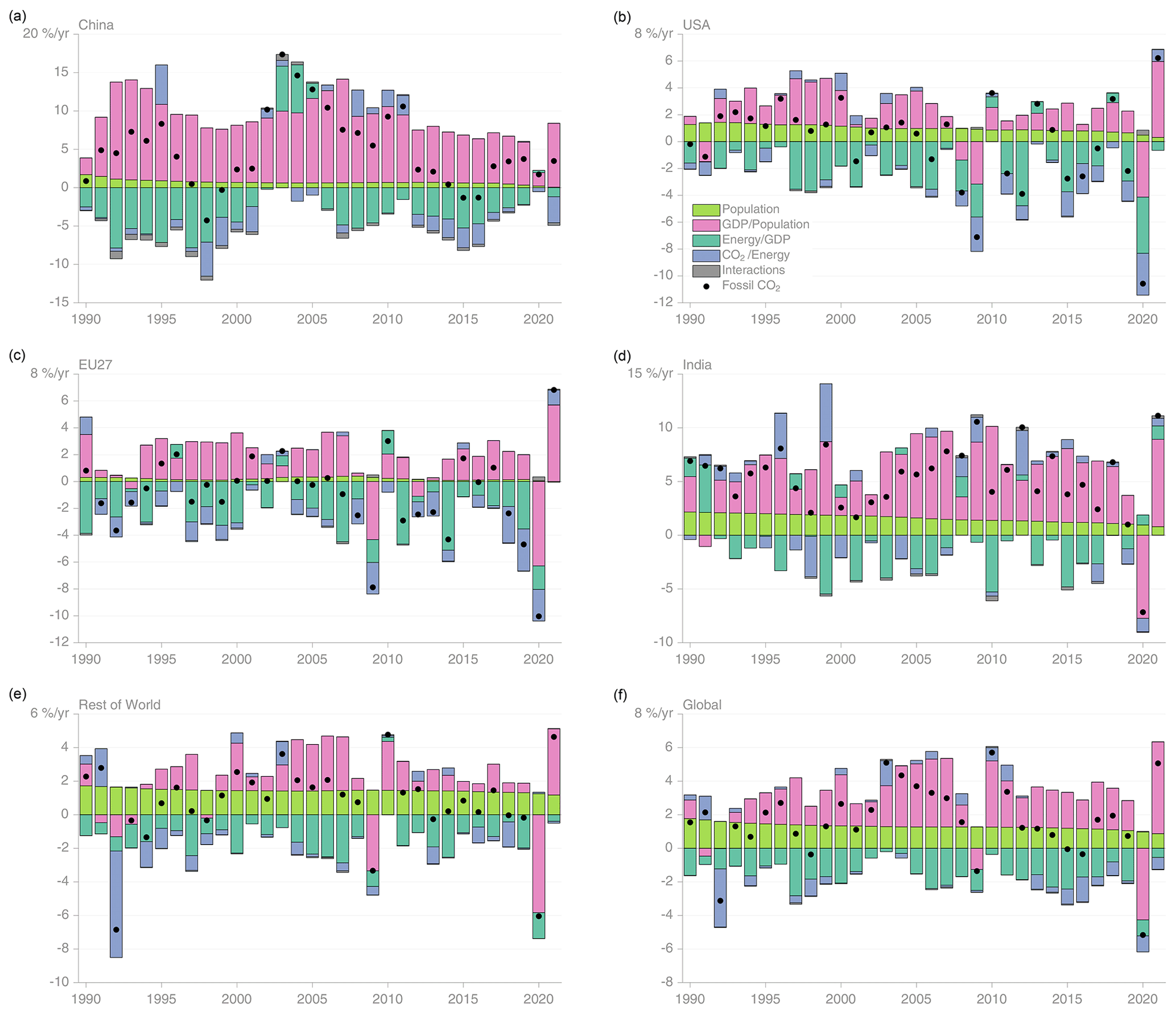
Figure 15Kaya decomposition of the main drivers of fossil CO2 emissions, considering population, GDP per person, energy per GDP, and CO2 emissions per energy, for China (a), the USA (b), the EU27 (c), India (d), the rest of the world (e), and the world (f). Black dots are the annual fossil CO2 emissions growth rate, coloured bars are the contributions from the different drivers. A general trend is that population and GDP growth put upward pressure on emissions, while energy per GDP and more recently CO2 emissions per energy put downward pressure on emissions. Both the COVID-19-induced changes during 2020 and the recovery in 2021 led to a stark contrast to previous years, with different drivers in each region.
In contrast, fossil CO2 emissions continue to grow in non-OECD countries, although the growth rate has slowed from almost 6 % per year during the 2000s to less than 2 % per year in the last decade. Representing 47 % of non-OECD emissions in 2021, a large part of this slowdown is due to China, which has seen emissions growth decline from nearly 10 % per year in the 2000s to 1.5 % per year in the last decade. Excluding China, non-OECD emissions grew at 3.3 % per year in the 2000s compared to 1.6 % per year in the last decade. Figure 15 shows that, compared to the previous decade, China has had weaker economic growth in the last decade and a higher decarbonization rate, with more rapid declines in energy per GDP that are now back to levels seen during the 1990s. India and the rest of the world have strong economic growth that is not offset by decarbonization or declines in energy per GDP, driving up fossil CO2 emissions. Despite the high deployment of renewables in some countries (e.g. India), fossil energy sources continue to grow to meet growing energy demand (Le Quéré et al., 2019).
Globally, fossil CO2 emissions growth is slowing, and this is due to the emergence of climate policy (Eskander and Fankhauser, 2020; Le Quere et al., 2019) and technological change, which is leading to a shift from coal to gas, growth in renewable energies, and reduced expansion of coal capacity. At the aggregated global level, decarbonization shows a strong and growing signal in the last decade, with smaller contributions from lower economic growth and declines in energy per GDP. Despite the slowing growth in global fossil CO2 emissions, emissions are still growing, but these are far from the reductions needed to meet the ambitious climate goals of the UNFCCC Paris Agreement.
We update the remaining carbon budget assessed by the IPCC AR6 (Canadell et al., 2021), accounting for the estimated 2020 to 2022 emissions from fossil fuel combustion (EFOS) and land-use changes (ELUC). From January 2023, the remaining carbon (50 % likelihood) for limiting global warming to 1.5, 1.7, and 2 ∘C is estimated to amount to 105, 200, and 335 GtC (380, 730, 1230 GtCO2). These numbers include an uncertainty based on model spread (as in IPCC AR6), which is reflected through the percent likelihood of exceeding the given temperature threshold. These remaining amounts correspond respectively to about 9, 18, and 30 years from the beginning of 2023 at the 2022 level of total CO2 emissions. Reaching net zero CO2 emissions by 2050 entails cutting total anthropogenic CO2 emissions by about 0.4 GtC (1.4 GtCO2) each year on average, comparable to the decrease observed in 2020 during the COVID-19 pandemic.
Table 10Major known sources of uncertainties in each component of the global carbon budget, defined as input data or processes that have a demonstrated effect of at least ±0.3 GtC yr−1.

a As a result of interactions between land use and climate. b The uncertainties in GATM have been estimated as ±0.2 GtC yr−1, although the conversion of the growth rate into a global annual flux assuming instantaneous mixing throughout the atmosphere introduces additional errors that have not yet been quantified.
Each year when the global carbon budget is published, each flux component is updated for all previous years to consider corrections that are the result of further scrutiny and verification of the underlying data in the primary input data sets. Annual estimates may be updated with improvements in data quality and timeliness (e.g. to eliminate the need for extrapolation of forcing data such as land use). Of all terms in the global budget, only the fossil CO2 emissions and the growth rate in atmospheric CO2 concentrations are based primarily on empirical inputs supporting annual estimates in this carbon budget. The carbon budget imbalance, while an imperfect measure, provides a strong indication of the limitations in observations in understanding and representing processes in models and/or in the integration of the carbon budget components.
The persistent unexplained variability in the carbon budget imbalance limits our ability to verify reported emissions (Peters et al., 2017) and suggests we do not yet have a complete understanding of the underlying carbon cycle dynamics on annual to decadal timescales. Resolving most of this unexplained variability should be possible through different and complementary approaches. First, as intended with our annual updates, the imbalance as an error term is reduced by improvements of individual components of the global carbon budget that follow from improving the underlying data and statistics and by improving the models through the resolution of some of the key uncertainties detailed in Table 10. Second, additional clues to the origin and processes responsible for the variability in the budget imbalance could be obtained through a closer scrutiny of carbon variability in light of other Earth system data (e.g. heat balance, water balance) and the use of a wider range of biogeochemical observations to better understand the land–ocean partitioning of the carbon imbalance (e.g. oxygen, carbon isotopes). Finally, additional information could also be obtained through higher resolution and process knowledge at the regional level and through the introduction of inferred fluxes such as those based on satellite CO2 retrievals. The limit of the resolution of the carbon budget imbalance is yet unclear, but has most certainly not yet been reached given the possibilities for improvements that lie ahead.
Estimates of global fossil CO2 emissions from different data sets are in relatively good agreement when the different system boundaries of these data sets are considered (Andrew, 2020a). But while estimates of EFOS are derived from reported activity data requiring much fewer complex transformations than some other components of the budget, uncertainties remain, and one reason for the apparently low variation between data sets is precisely the reliance on the same underlying reported energy data. The budget excludes some sources of fossil CO2 emissions, which available evidence suggests are relatively small (< 1 %). We have added emissions from lime production in China and the US, but these are still absent in most other non-Annex I countries and before 1990 in other Annex I countries.
Estimates of ELUC suffer from a range of intertwined issues, including the poor quality of historical land cover and land-use change maps, the rudimentary representation of management processes in most models, and the confusion in methodologies and boundary conditions used across methods (e.g. Arneth et al., 2017; Pongratz et al., 2014; Bastos et al., 2021; see also Appendix D4 on the loss of sink capacity). Uncertainties in current and historical carbon stocks in soils and vegetation also add uncertainty in the ELUC estimates. Unless a major effort to resolve these issues is made, little progress is expected in the resolution of ELUC. This is particularly concerning given the growing importance of ELUC for climate mitigation strategies and the large issues in the quantification of the cumulative emissions over the historical period that arise from large uncertainties in ELUC.
By adding the DGVM estimates of CO2 fluxes due to environmental change from countries' managed forest areas (part of SLAND in this budget) to the budget ELUC estimate, we successfully reconciled the large gap between our ELUC estimate and the land-use flux from NGHGIs using the approach described in Grassi et al. (2021) for a future scenario and in Grassi et al. (2022b) using data from the Global Carbon Budget 2021. The updated data presented here can be used as potential adjustment in the policy context, e.g. to help assessing the collective countries' progress towards the goal of the Paris Agreement and avoiding double accounting of the sink in managed forests. In the absence of this adjustment, collective progress would hence appear better than it is (Grassi et al., 2021). The need of such adjustment whenever a comparison between LULUCF fluxes reported by countries and the global emission estimates of the IPCC is attempted is recommended also in the recent UNFCCC Synthesis report for the first Global Stocktake (UNFCCC, 2022). However, this adjustment should be seen as a short-term and pragmatic fix based on existing data, rather than a definitive solution to bridge the differences between global models and national inventories. Additional steps are needed to understand and reconcile the remaining differences, some of which are relevant at the country level (Grassi et al., 2022b; Schwingshackl et al., 2022).
The comparison of GOBMs, data products, and inversions highlights a substantial discrepancy in the Southern Ocean (Fig. 13, Hauck et al., 2020). A large part of the uncertainty in the mean fluxes stems from the regional distribution of the river flux adjustment term. The current distribution (Aumont et al., 2001) is based on one model study yielding the largest riverine outgassing flux south of 20∘ S, whereas a recent study, also based on one model, simulates the largest share of the outgassing to occur in the tropics (Lacroix et al., 2020). The long-standing sparse data coverage of fCO2 observations in the Southern Hemisphere compared to the Northern Hemisphere (e.g. Takahashi et al., 2009) continues to exist (Bakker et al., 2016, 2022, Fig. B1) and to lead to substantially higher uncertainty in the SOCEAN estimate for the Southern Hemisphere (Watson et al., 2020; Gloege et al., 2021). This discrepancy, which also hampers model improvement, points to the need for increased high-quality fCO2 observations, especially in the Southern Ocean. At the same time, model uncertainty is illustrated by the large spread of individual GOBM estimates (indicated by shading in Fig. 13) and highlights the need for model improvement. The diverging trends in SOCEAN from different methods is a matter of concern, which is unresolved. The assessment of the net land–atmosphere exchange from DGVMs and atmospheric inversions also shows substantial discrepancy, particularly for the estimate of the total land flux over the northern extratropics. This discrepancy highlights the difficulty to quantify complex processes (CO2 fertilization, nitrogen deposition and fertilizers, climate change and variability, land management, etc.) that collectively determine the net land CO2 flux. Resolving the differences in the Northern Hemisphere land sink will require the consideration and inclusion of larger volumes of observations.
We provide metrics for the evaluation of the ocean and land models and the atmospheric inversions (Figs. B2 to B4). These metrics expand the use of observations in the global carbon budget, helping (1) to support improvements in the ocean and land carbon models that produce the sink estimates and (2) to constrain the representation of key underlying processes in the models and allocate the regional partitioning of the CO2 fluxes. However, GOBMs skills have changed little since the introduction of the ocean model evaluation. The additional simulation allows for direct comparison with interior ocean anthropogenic carbon estimates and suggests that the models underestimate anthropogenic carbon uptake and storage. This is an initial step towards the introduction of a broader range of observations that we hope will support continued improvements in the annual estimates of the global carbon budget.
We assessed before that a sustained decrease of −1 % in global emissions could be detected at the 66 % likelihood level after a decade only (Peters et al., 2017). Similarly, a change in behaviour of the land and/or ocean carbon sink would take as long to detect and much longer if it emerges more slowly. Continuing with reducing the carbon imbalance on annual to decadal timescales, regionalizing the carbon budget, and integrating multiple variables are powerful ways to shorten the detection limit and ensure the research community can rapidly identify issues of concern in the evolution of the global carbon cycle under the current rapid and unprecedented changing environmental conditions.
The estimation of global CO2 emissions and sinks is a major effort by the carbon cycle research community that requires a careful compilation and synthesis of measurements, statistical estimates, and model results. The delivery of an annual carbon budget serves two purposes. First, there is a large demand for up-to-date information on the state of the anthropogenic perturbation of the climate system and its underpinning causes. A broad stakeholder community relies on the data sets associated with the annual carbon budget including scientists, policy makers, businesses, journalists, and non-governmental organizations engaged in adapting to and mitigating human-driven climate change. Second, over the last decades we have seen unprecedented changes in the human and biophysical environments (e.g. changes in the growth of fossil fuel emissions, impacts of the COVID-19 pandemic, Earth's warming, and strength of the carbon sinks), which call for frequent assessments of the state of the planet, a better quantification of the causes of changes in the contemporary global carbon cycle, and an improved capacity to anticipate its evolution in the future. Building this scientific understanding to meet the extraordinary climate mitigation challenge requires frequent, robust, transparent, and traceable data sets and methods that can be scrutinized and replicated. This paper, via “living data”, helps to keep track of new budget updates.
The data presented here are made available in the belief that their wide dissemination will lead to greater understanding and new scientific insights of how the carbon cycle works, how humans are altering it, and how we can mitigate the resulting human-driven climate change. Full contact details and information on how to cite the data shown here are given at the top of each page in the accompanying database and summarized in Table 2.
The accompanying database includes three Excel files organized into the following spreadsheets.
The file Global_Carbon_Budget_2022v0.1.xlsx includes the following items:
-
summary;
-
the global carbon budget (1959–2021);
-
the historical global carbon budget (1750–2021);
-
global CO2 emissions from fossil fuels and cement production by fuel type and the per capita emissions (1850–2021);
-
CO2 emissions from land-use change from the individual bookkeeping models (1959–2021);
-
ocean CO2 sink from the individual ocean models and fCO2-based products (1959–2021);
-
terrestrial CO2 sink from the individual DGVMs (1959–2021);
-
cement carbonation CO2 sink (1959–2021).
The file National_Fossil_Carbon_Emissions_2022v0.1.xlsx includes the following items:
-
summary;
-
territorial country CO2 emissions from fossil fuels and cement production (1850–2021);
-
consumption country CO2 emissions from fossil fuels and cement production and emissions transfer from the international trade of goods and services (1990–2020) using CDIAC/UNFCCC data as reference;
-
emissions transfers (consumption minus territorial emissions; 1990–2020);
-
country definitions.
The file National_LandUseChange_Carbon_Emissions_2022v0.1xlsx includes the following items:
-
summary
-
territorial country CO2 emissions from land-use change (1850–2021) from three bookkeeping models;
All three spreadsheets are published by the Integrated Carbon Observation System (ICOS) Carbon Portal and are available at https://doi.org/10.18160/GCP-2022 (Friedlingstein et al., 2022b). National emissions data are also available from the Global Carbon Atlas (http://www.globalcarbonatlas.org/, last access: 25 September 2022) and from Our World in Data (https://ourworldindata.org/co2-emissions, last access: 25 September 2022).
Table A1Comparison of the processes included in the bookkeeping method and DGVMs in their estimates of ELUC and SLAND. See Table 4 for model references. All models include deforestation and forest regrowth after abandonment of agriculture (or from afforestation activities on agricultural land). Processes relevant for ELUC are only described for the DGVMs used with land-cover change in this study. Here we use the term “DGVM” in the broadest sense in terms of global vegetation models which are able to dynamically adjust to imposed land use and land-use change (LULCC).
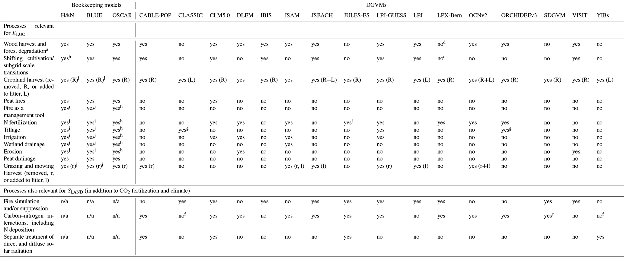
Table A2Comparison of the processes and model set-up for the Global Ocean Biogeochemistry Models for their estimates of SOCEAN. See Table 4 for model references.
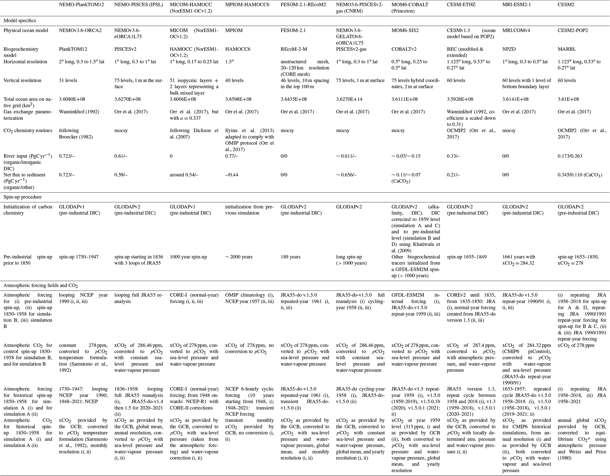
Table A3Description of ocean data products used for assessment of SOCEAN. See Table 4 for references.
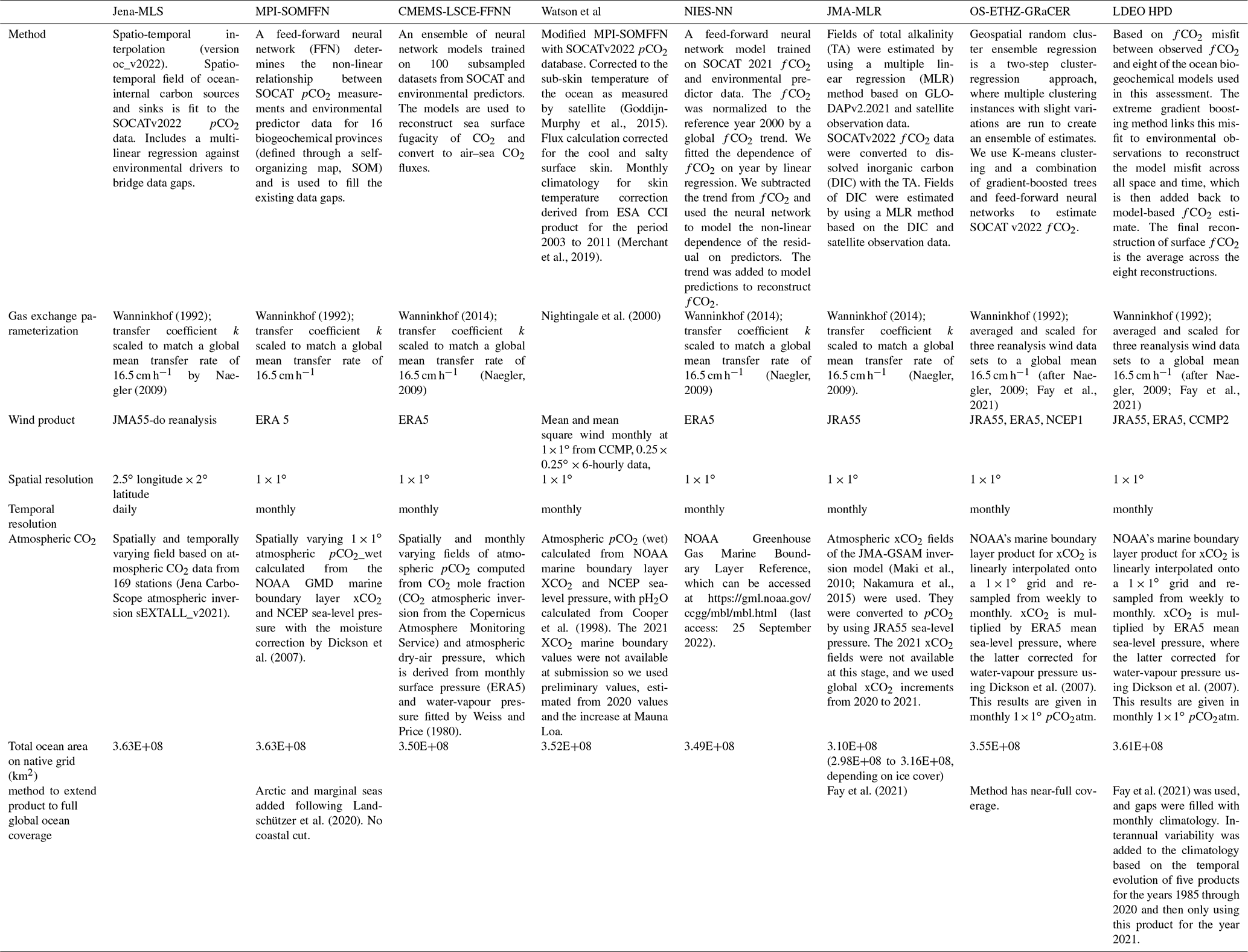
Table A4Comparison of the inversion set-up and input fields for the atmospheric inversions. Atmospheric inversions see the full CO2 fluxes, including the anthropogenic and pre-industrial fluxes. Hence, they need to be adjusted for the pre-industrial flux of CO2 from the land to the ocean that is part of the natural carbon cycle before they can be compared with SOCEAN and SLAND from process models. See Table 4 for references.
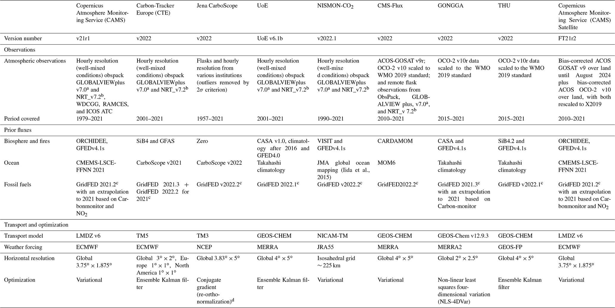
a https://doi.org/10.25925/20210801 (Schuldt et al., 2021). b https://doi.org/10.25925/20220624 (Schuldt et al., 2022). c GCP-GridFED v2021.2, v2021.3, v2022.1, and v2022.2 (Jones et al., 2022) are updates through the year 2021 of the GCP-GridFED dataset presented by Jones et al. (2021). d Ocean prior is not optimized.
Table A5Attribution of fCO2 measurements for the year 2021 included in SOCATv2022 (Bakker et al., 2016, 2022) to inform ocean fCO2-based data products.
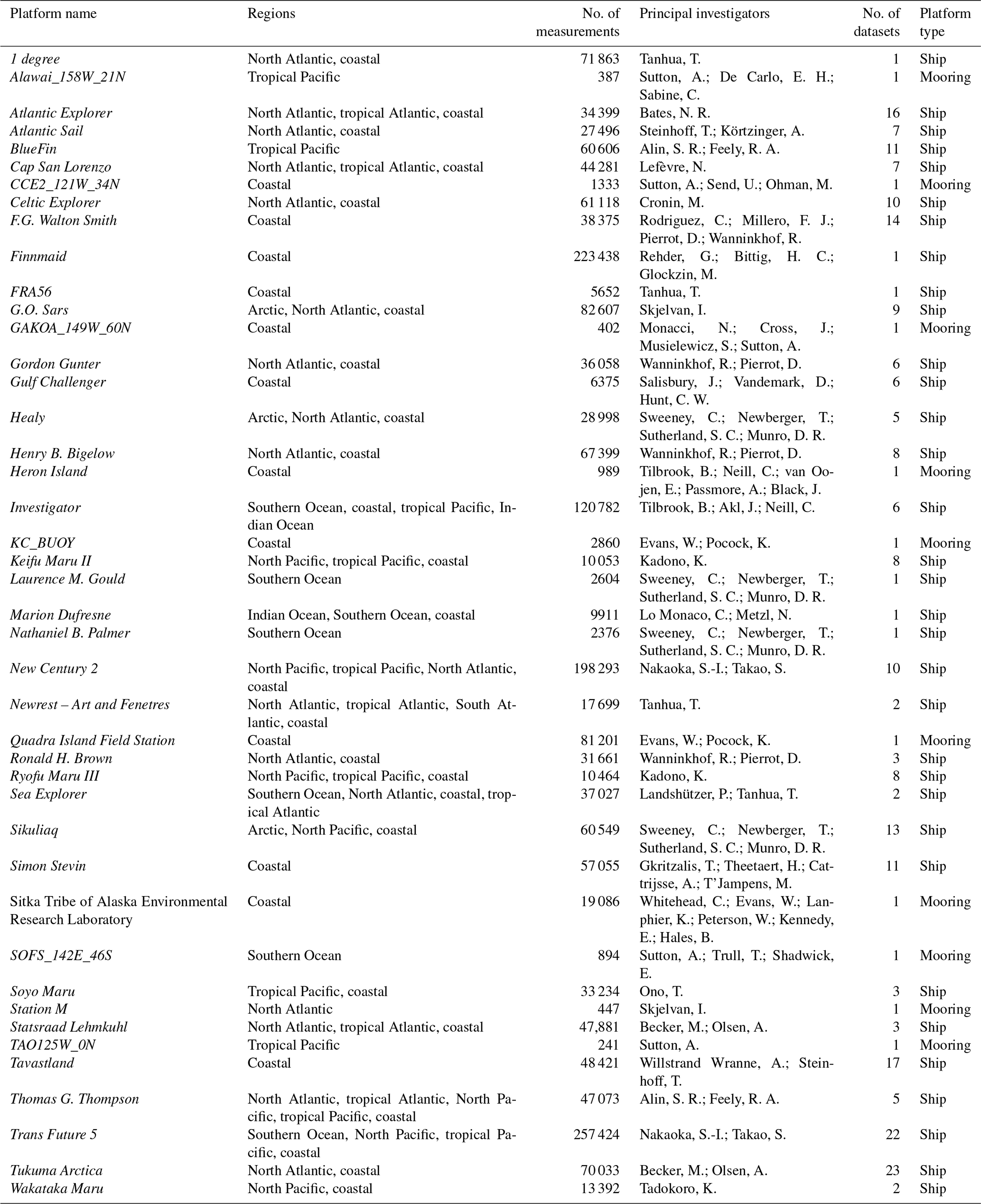
Table A6Aircraft measurement programmes archived by Cooperative Global Atmospheric Data Integration Project (CGADIP; Schuldt et al., 2021, 2022) that contribute to the evaluation of the atmospheric inversions (Fig. B4).
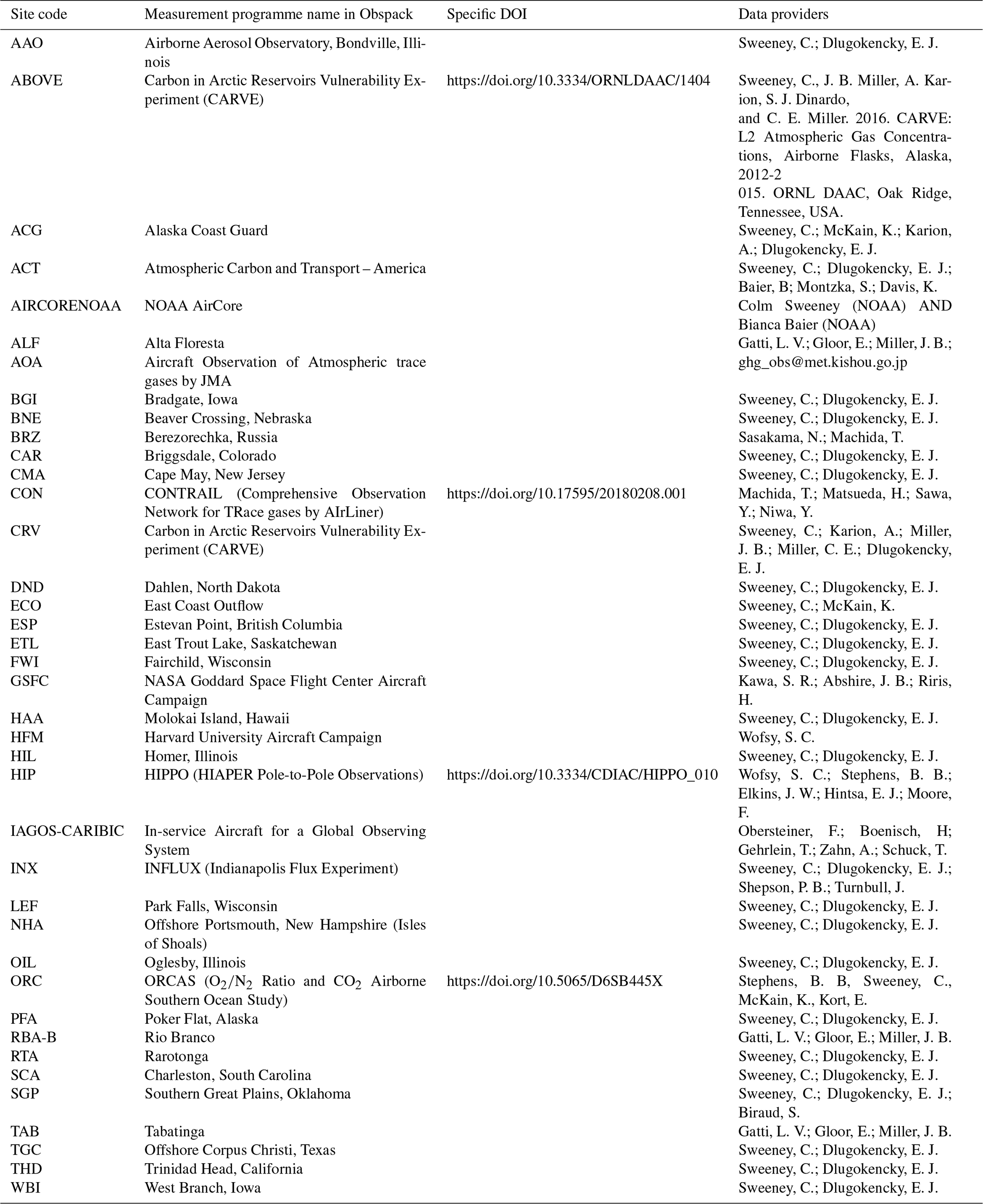
Table A7Main methodological changes in the global carbon budget since first publication. Methodological changes introduced in one year are kept for the following years unless noted. Empty cells mean there were no methodological changes introduced that year.
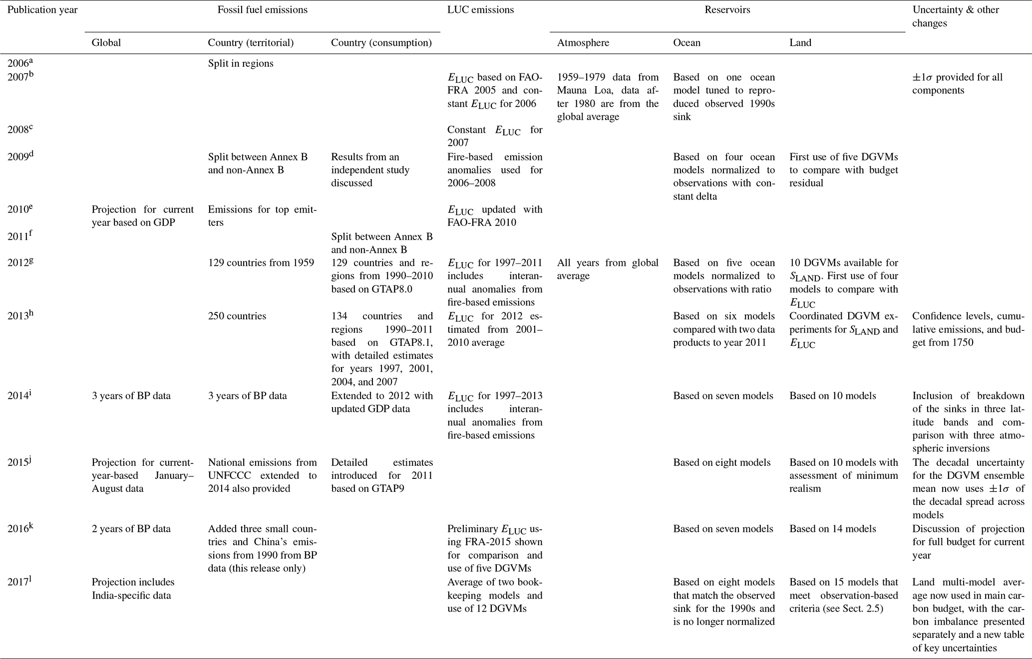
a Raupach et al. (2007). b Canadell et al. (2007). c GCP (2007). d Le Quéré et al. (2009). e Friedlingstein et al. (2010). f Peters et al. (2012b). g Le Quéré et al. (2013); Peters et al. (2013). h Le Quéré et al. (2014). i Le Quéré et al. (2015a); j Le Quéré et al. (2015b). k Le Quéré et al. (2016). l Le Quéré et al. (2018a).
Table A8Mapping of global carbon cycle models land flux definitions to the definition of the LULUCF net flux used in national reporting to UNFCCC. Non-intact lands are used here as proxy for “managed lands” in the country reporting; national greenhouse gas inventories (NGHGI) are gap filled (see Sect. C2.3 for details). Where available, we provide independent estimates of certain fluxes for comparison (values are in GtC yr−1).
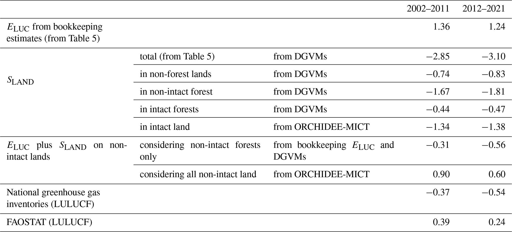
Table A9Funding supporting the production of the various components of the global carbon budget in addition to the authors' supporting institutions (see the Acknowledgements for further details).
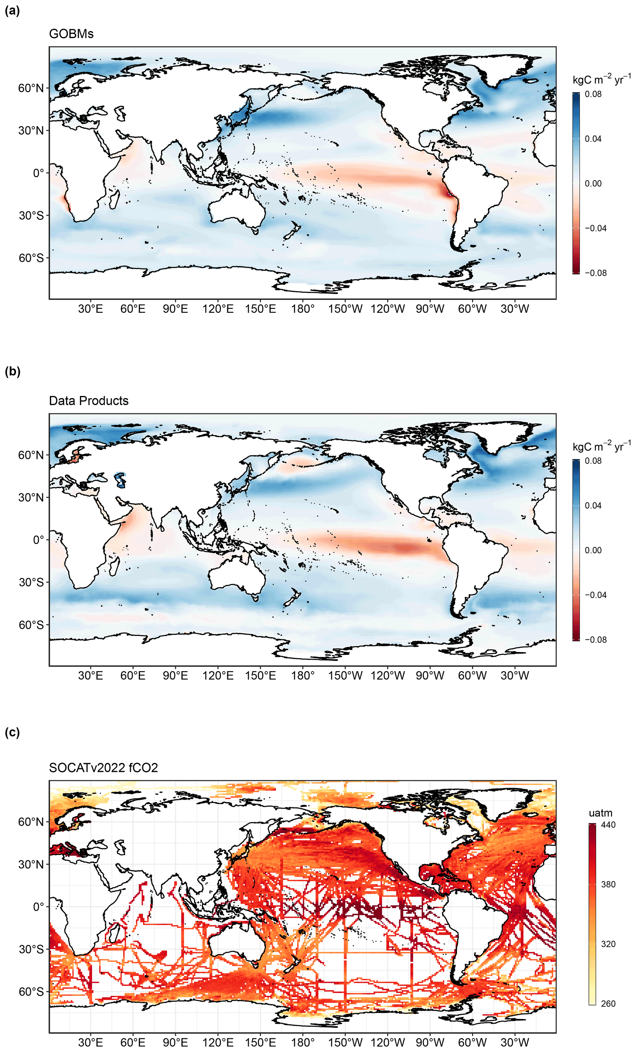
Figure B1Ensemble mean air–sea CO2 flux from (a) global ocean biogeochemistry models and (b) fCO2-based data products, averaged over the 2012–2021 period (kgC m−2 yr−1). Positive numbers indicate a flux into the ocean. (c) Gridded SOCAT v2022 fCO2 measurements, averaged over the 2012–2021 period (µatm). In (a), model simulation A is shown. The data products represent the contemporary flux, i.e. including outgassing of riverine carbon, which is estimated to amount to 0.65 GtC yr−1 globally.
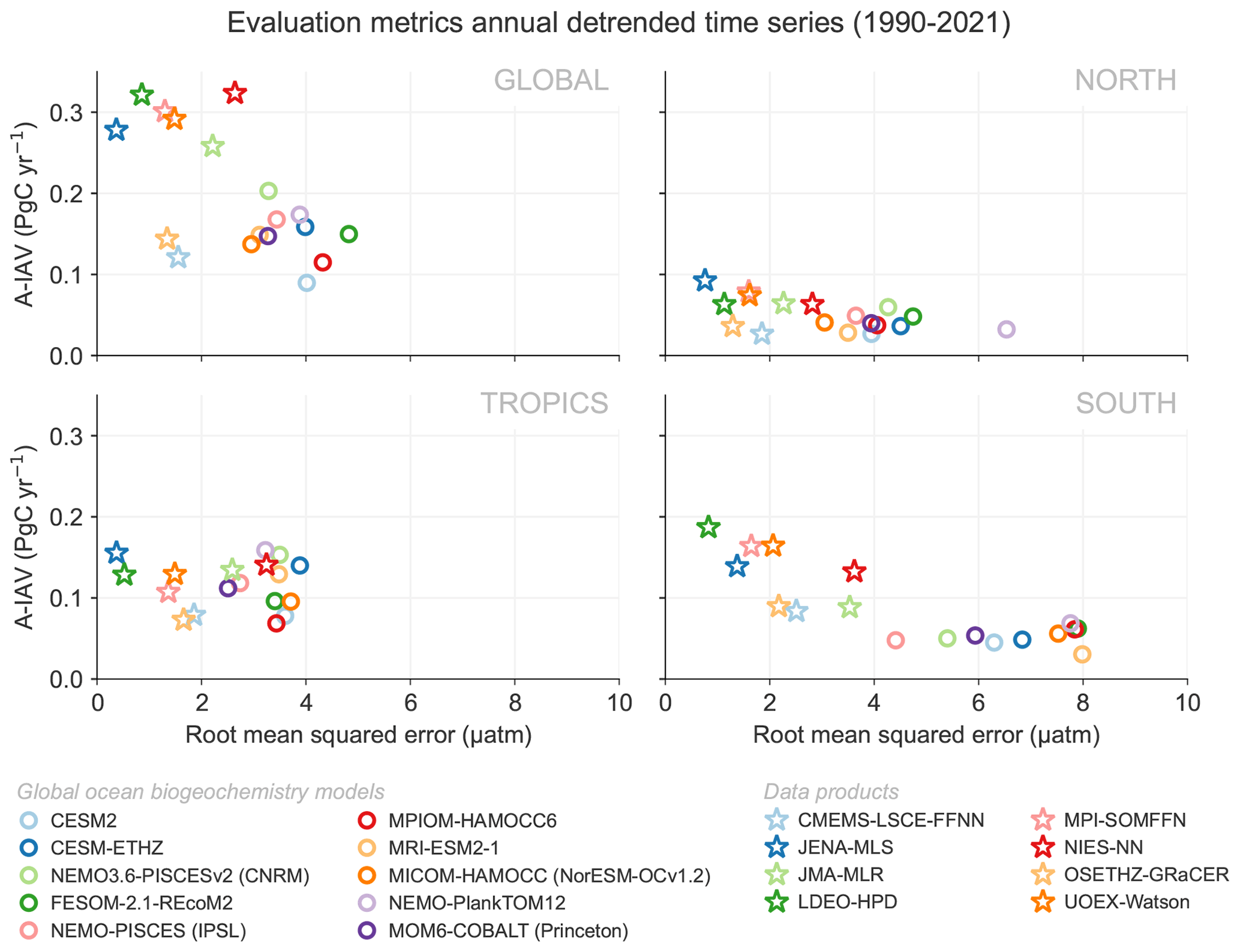
Figure B2Evaluation of the GOBMs and data products using the root-mean-squared error (RMSE) for the period 1990 to 2021 between the individual surface ocean fCO2 mapping schemes and the SOCAT v2022 database. The y axis shows the amplitude of the interannual variability of the air–sea CO2 flux (A-IAV), taken as the standard deviation of the detrended annual time series. Results are presented for the globe, northern extratropics (> 30∘ N), tropics (30∘ S–30∘ N), and southern extratropics (< 30∘ S) for the GOBMs (see legend, circles) and for the fCO2-based data products (star symbols). The fCO2-based data products use the SOCAT database and are therefore not independent of the data (see Sect. 2.4.1).

Figure B3Evaluation of the DGVMs using the International Land Model Benchmarking system (ILAMB; Collier et al., 2018) (left) absolute skill scores and (right) skill scores relative to other models. The benchmarking is done with observations for vegetation biomass (Saatchi et al., 2011; and global carbon unpublished data; Avitabile et al., 2016), GPP (Jung et al., 2010; Lasslop et al., 2010), leaf area index (De Kauwe et al., 2011; Myneni et al., 1997), ecosystem respiration (Jung et al., 2010; Lasslop et al., 2010), soil carbon (Hugelius et al., 2013; Todd-Brown et al., 2013), evapotranspiration (De Kauwe et al., 2011), and runoff (Dai and Trenberth, 2002). For each model–observation comparison a series of error metrics are calculated. Scores are then calculated as an exponential function of each error metric. Finally, for each variable the multiple scores from different metrics and observational data sets are combined to give the overall variable scores shown in the left panel. Overall variable scores increase from 0 to 1 with improvements in model performance. The set of error metrics vary with data set and can include metrics based on the period mean, bias, root-mean-squared error, spatial distribution, interannual variability and seasonal cycle. The relative skill score shown in the right panel is a Z score, which indicates in units of standard deviation the model scores relative to the multi-model mean score for a given variable. Grey boxes represent missing model data.
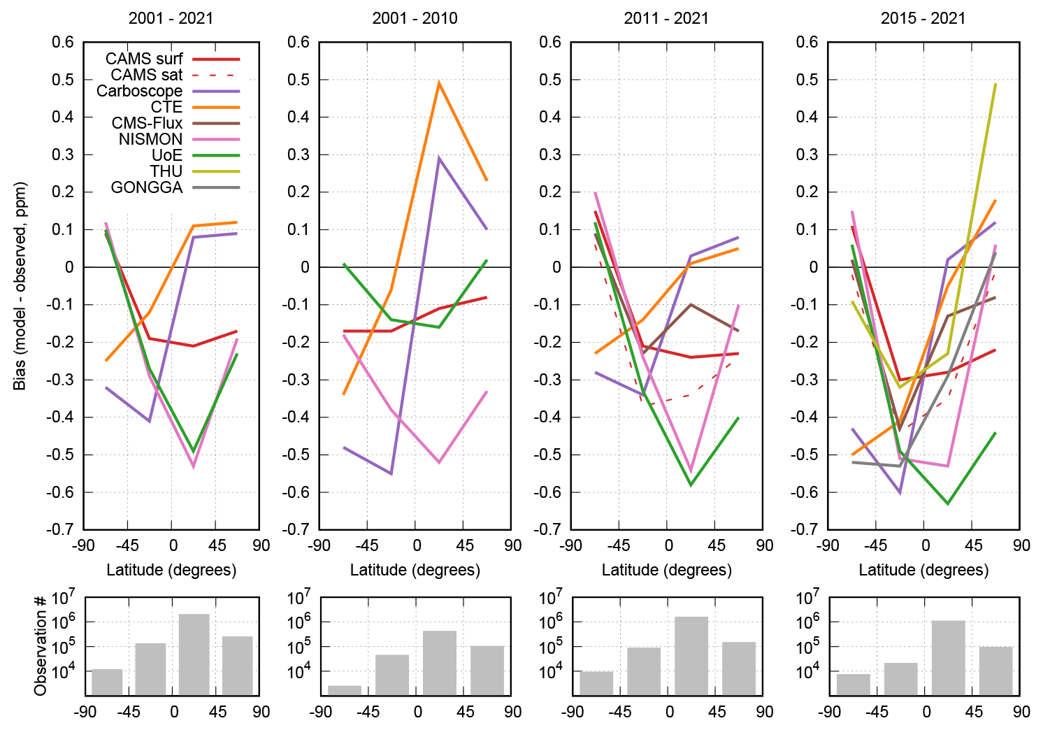
Figure B4Evaluation of the atmospheric inversion products. The mean of the model minus observations is shown for four latitude bands in four periods: (first panel) 2001–2021, (second panel) 2001–2010, (third panel) 2011–2021, and (fourth panel) 2015–2021. The nine systems are compared to independent CO2 measurements made aboard aircraft over many areas of the world between 2 and 7 km above sea level. Aircraft measurements archived in the Cooperative Global Atmospheric Data Integration Project (Schuldt et al., 2021, 2022) from sites, campaigns, or programmes that have not been assimilated and cover at least 9 months (except for SH programmes) between 2001 and 2021 have been used to compute the biases of the differences in four 45∘ latitude bins. Land and ocean data are used without distinction, and observation density varies strongly with latitude and time, as seen in the lower panels.
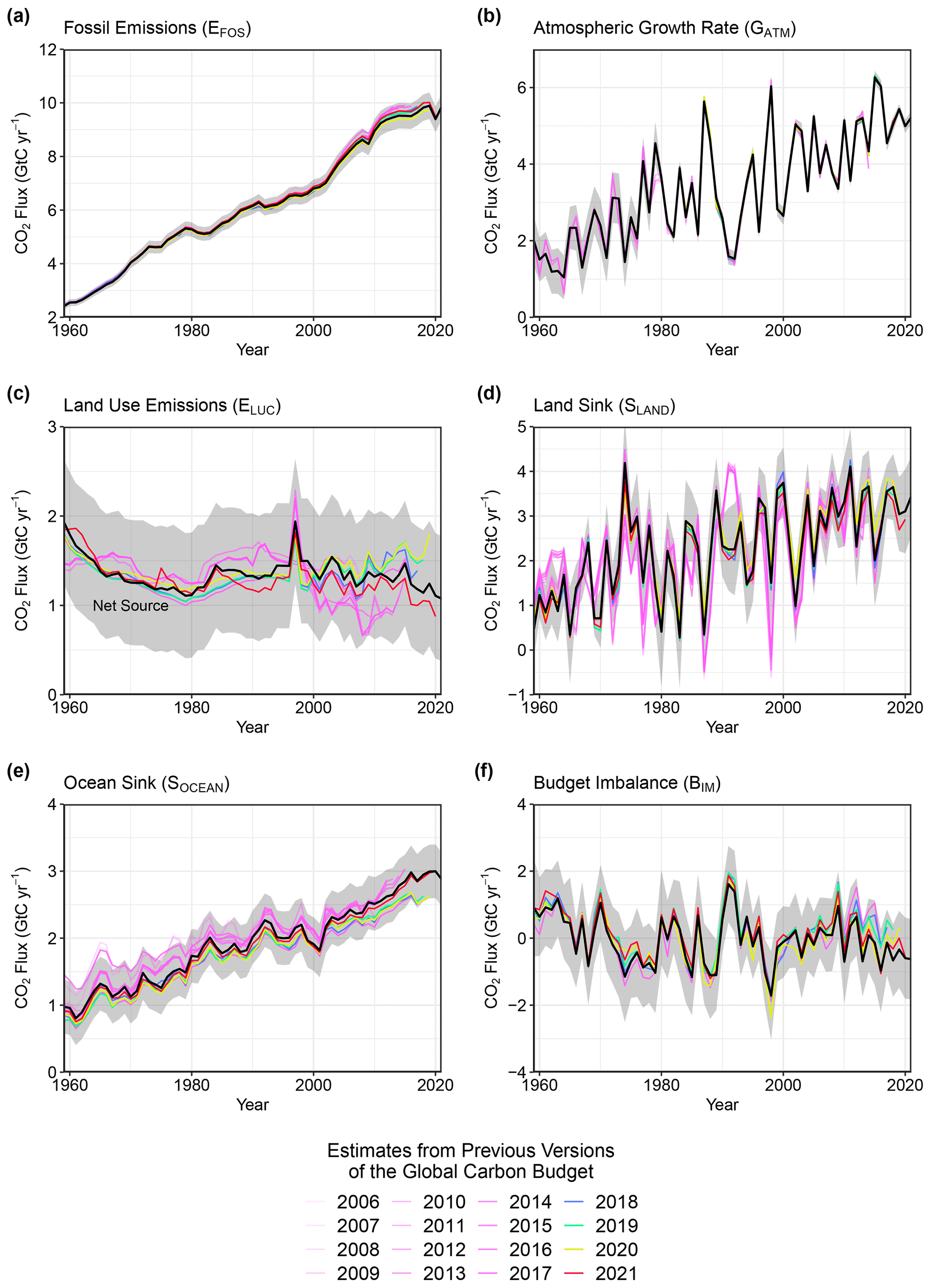
Figure B5Comparison of the estimates of each component of the global carbon budget in this study (black line) with the estimates released annually by the GCP since 2006. Grey shading shows the uncertainty bounds representing ±1 standard deviation of the current global carbon budget based on the uncertainty assessments described in Appendix C. CO2 emissions from (a) fossil CO2 emissions (EFOS) and (b) land-use change (ELUC) and their partitioning among (c) the atmosphere (GATM), (d) land (SLAND), and (e) ocean (SOCEAN). See the legend for the corresponding years and Tables 3 and A7 for references. The budget year corresponds to the year when the budget was first released (all values are in GtC yr−1).
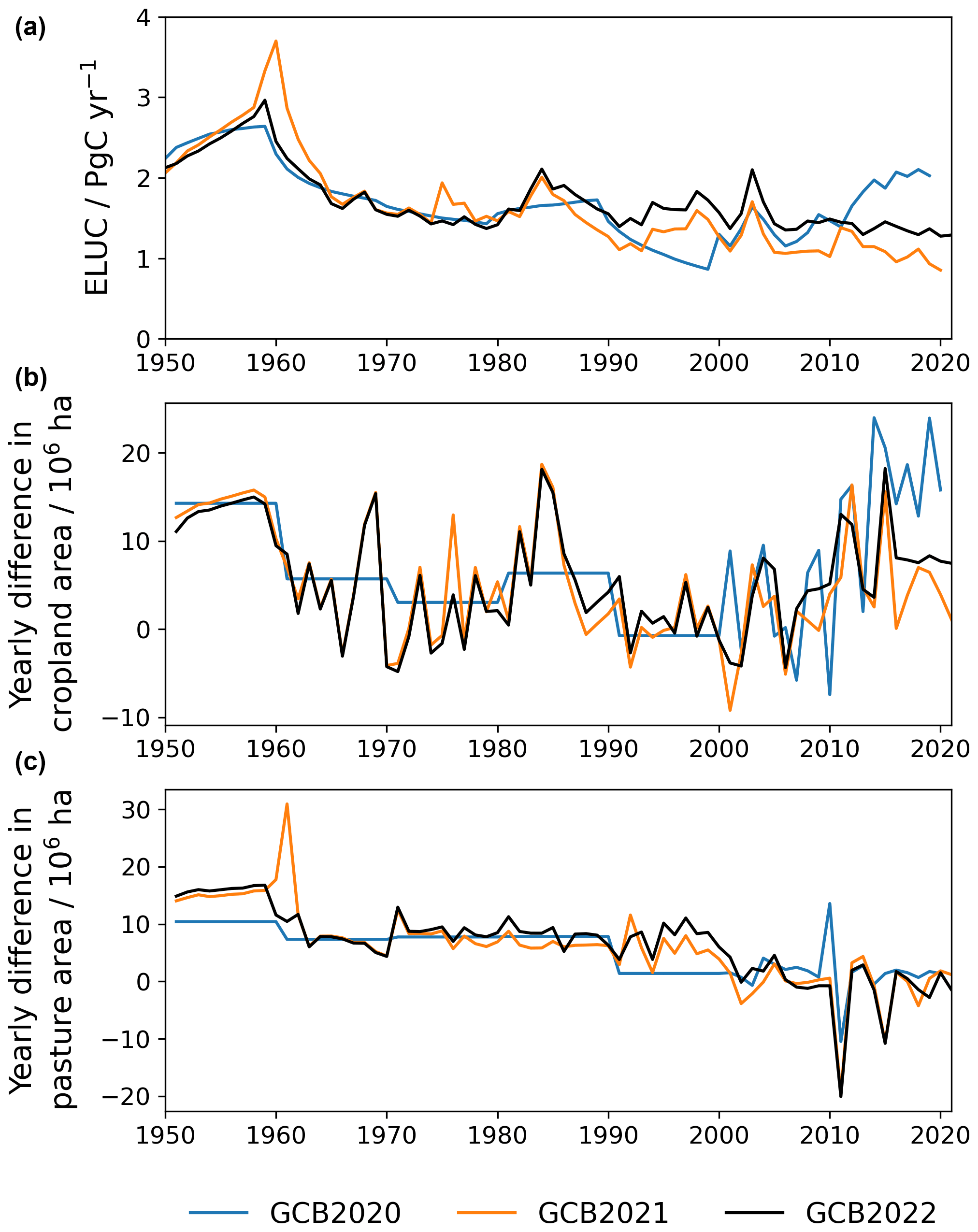
Figure B6Differences in the HYDE/LUH2 land-use forcing used for the global carbon budgets GCB2020 (Friedlingstein et al., 2021), GCB2021 (Friedlingstein et al., 2022a), and GCB2022 (Friedlingstein et al., 2022b). Shown are year-to-year changes in cropland area (b) and pasture area (c). To illustrate the relevance of the update in the land-use forcing to the recent trends in ELUC, the top panel shows the land-use emission estimate from the bookkeeping model BLUE (original model output, i.e. excluding peat fire and drainage emissions).
C1 Methodology: fossil fuel CO2 emissions (EFOS)
C1.1 Cement carbonation
From the moment it is created, cement begins to absorb CO2 from the atmosphere, a process known as “cement carbonation”. We estimate this CO2 sink, from 1931 onwards as the average of two studies in the literature (Cao et al., 2020; Guo et al., 2021). The Global Cement and Concrete Association reports a much lower carbonation rate, but this is based on the highly conservative assumption of 0 % mortar (GCCA, 2021). Modelling cement carbonation requires estimation of a large number of parameters, including the different types of cement material in different countries, the lifetime of the structures before demolition, the lifetime of cement waste after demolition, and the volumetric properties of structures (Xi et al., 2016). Lifetime is an important parameter because demolition results in the exposure of new surfaces to the carbonation process. The main reasons for differences between the two studies appear to be the assumed lifetimes of cement structures and the geographic resolution, but the uncertainty bounds of the two studies overlap.
C1.2 Emissions embodied in goods and services
CDIAC, UNFCCC, and BP national emission statistics “include greenhouse gas emissions and removals taking place within national territory and offshore areas over which the country has jurisdiction” (Rypdal et al., 2006) and are called territorial emission inventories. Consumption-based emission inventories allocate emissions to products that are consumed within a country and are conceptually calculated as the territorial emissions minus the “embodied” territorial emissions to produce exported products plus the emissions in other countries to produce imported products (consumption is equal to territorial minus exports plus imports). Consumption-based emission attribution results (e.g. Davis and Caldeira, 2010) provide additional information to territorial-based emissions that can be used to understand emission drivers (Hertwich and Peters, 2009) and quantify emission transfers by the trade of products between countries (Peters et al., 2011b). The consumption-based emissions have the same global total but reflect the trade-driven movement of emissions across the Earth's surface in response to human activities. We estimate consumption-based emissions from 1990–2020 by enumerating the global supply chain using a global model of the economic relationships between economic sectors within and between every country (Andrew and Peters, 2013; Peters et al., 2011a). Our analysis is based on the economic and trade data from the Global Trade and Analysis Project (GTAP; Narayanan et al., 2015), and we make detailed estimates for the years 1997 (GTAP version 5); 2001 (GTAP6); and 2004, 2007, 2011, and 2014 (GTAP10.0a), covering 57 sectors and 141 countries and regions. The detailed results are then extended into an annual time series from 1990 to the latest year of the gross domestic product (GDP) data (2020 in this budget) using GDP data by expenditure in current exchange rate of US dollars (USD; from the UN National Accounts main aggregates database; UN, 2021) and time series of trade data from GTAP (based on the methodology in Peters et al., 2011a). We estimate the sector-level CO2 emissions using the GTAP data and methodology, add the flaring and cement emissions from our fossil CO2 dataset, and then scale the national totals (excluding bunker fuels) to match the emission estimates from the carbon budget. We do not provide a separate uncertainty estimate for the consumption-based emissions; however, based on model comparisons and sensitivity analysis, they are unlikely to be significantly different than for the territorial emission estimates (Peters et al., 2012a).
C1.3 Uncertainty assessment for EFOS
We estimate the uncertainty of the global fossil CO2 emissions at ±5 % (scaled down from the published ±10 % at ±2σ to the use of ± 1σ bounds reported here; Andres et al., 2012). This is consistent with a more detailed analysis of uncertainty of ±8.4 % at ±2σ (Andres et al., 2014) and at the high end of the range of ±5 %–10 % at ±2σ reported by (Ballantyne et al., 2015). This includes an assessment of uncertainties in the amounts of fuel consumed, the carbon and heat contents of fuels, and the combustion efficiency. While we consider a fixed uncertainty of ±5 % for all years, the uncertainty as a percentage of emissions is growing with time because of the larger share of global emissions from emerging economies and developing countries (Marland et al., 2009). Generally, emissions from mature economies with good statistical processes have an uncertainty of only a few percent (Marland, 2008), while emissions from strongly developing economies such as China have uncertainties of around ±10 % (for ±1σ; Gregg et al., 2008; Andres et al., 2014). Uncertainties in emissions are likely to be mainly systematic errors related to underlying biases of energy statistics and to the accounting method used by each country.
C1.4 Growth rate in emissions
We report the annual growth rate in emissions for adjacent years (in percent per year) by calculating the difference between the 2 years and then normalizing to the emissions in the first year: ( %. We apply a leap-year adjustment where relevant to ensure valid interpretations of annual growth rates. This affects the growth rate by about 0.3 % per year () and causes calculated growth rates to go up approximately 0.3 % if the first year is a leap year and down 0.3 % if the second year is a leap year. The relative growth rate of EFOS over time periods of greater than 1 year can be rewritten using its logarithm equivalent as follows:
Here we calculate relative growth rates in emissions for multi-year periods (e.g. a decade) by fitting a linear trend to ln (EFOS) in Eq. (2), reported in percent per year.
C1.5 Emissions projection for 2022
To gain insight into emission trends for 2022, we provide an assessment of global fossil CO2 emissions, EFOS, by combining individual assessments of emissions for China, USA, the EU, and India (the four countries/regions with the largest emissions) and the rest of the world.
The methods are specific to each country or region, as described in detail below.
China
We use a regression between monthly data for each fossil fuel and cement and annual data for consumption of fossil fuels or production of cement to project full-year growth in fossil fuel consumption and cement production. The monthly data for each product consists of the following elements.
-
Coal. This product uses a proprietary estimate for monthly consumption of main coal types from SX Coal.
-
Oil. The product uses production data from the National Bureau of Statistics (NBS), plus net imports from the China Customs Administration (i.e. gross supply of oil, not including inventory changes).
-
Natural gas. This product uses the same source as for oil.
-
Cement. This product uses production data from NBS.
For oil, we use data for production and net imports of refined oil products rather than crude oil. This choice is made because refined products are one step closer to actual consumption and because crude oil can be subject to large market-driven and strategic inventory changes that are not captured by available monthly data.
For each fuel and cement, we make a Bayesian linear regression between year-on-year cumulative growth in supply (production for cement) and full-year growth in consumption (production for cement) from annual consumption data. In the regression model, the growth rate in annual consumption (production for cement) is modelled as a regression parameter multiplied by the cumulative year-on-year growth rate from the monthly data through July of each year for past years (through 2021). We use broad Gaussian distributions centred around 1 as priors for the ratios between annual and through-July growth rates. We then use the posteriors for the growth rates together with cumulative monthly supply or production data through July of 2022 to produce a posterior predictive distribution for the full-year growth rate for fossil fuel consumption and cement production in 2022.
If the growth in supply or production through July were an unbiased estimate of the full-year growth in consumption or production, the posterior distribution for the ratio between the monthly and annual growth rates would be centred around 1. However, in practice the ratios are different from 1 (in most cases below 1). This is a result of various biassing factors such as uneven evolution in the first and second half of each year, inventory changes that are somewhat anti-correlated with production and net imports, differences in statistical coverage, and other factors that are not captured in the monthly data.
For fossil fuels, the mean of the posterior distribution is used as the central estimate for the growth rate in 2022, while the edges of a 68 % credible interval (analogous to a 1σ confidence interval) are used for the upper and lower bounds.
For cement, the evolution from January to July has been highly atypical owing to the ongoing turmoil in the construction sector, and the results of the regression analysis are heavily biased by equally atypical but different dynamics in 2021. For this reason, we use an average of the results of the regression analysis and the plain growth in cement production through July 2022, since this results in a growth rate that seems more plausible and in line with where the cumulative cement production appears to be headed at the time of writing.
USA
We use emissions estimated by the U.S. Energy Information Administration (EIA) in their Short-Term Energy Outlook (STEO) for emissions from fossil fuels to get both year-to-date (YTD) information and a full-year projection (EIA, 2022). The STEO also includes a near-term forecast based on an energy forecasting model that is updated monthly (last update with preliminary data through August 2022) and takes into account expected temperatures, household expenditures by fuel type, energy markets, policies, and other effects. We combine this with our estimate of emissions from cement production using the monthly US cement clinker production data from USGS for January–June 2022, assuming changes in cement production over the first part of the year apply throughout the year.
India
We use monthly emissions estimates for India updated from Andrew (2020b) through July 2022. These estimates are derived from many official monthly energy and other activity data sources to produce direct estimates of national CO2 emissions without the use of proxies. Emissions from coal are then extended to August using a regression relationship based on power generated from coal, coal dispatches by Coal India Ltd., the composite Purchasing Managers' Index, time, and days per month. For the last 3–5 months of the year, each series is extrapolated assuming typical trends.
EU
We use a refinement to the methods presented by Andrew (2021), deriving emissions from monthly energy data reported by Eurostat. Some data gaps are filled using data from the Joint Organizations Data Initiative (JODI, 2022). Sub-annual cement production data are limited, but data for Germany and Poland, the two largest producers, suggest a small decline. For fossil fuels this provides estimates through July. We extend coal emissions through August using a regression model built from generation of power from hard coal, power from brown coal, total power generation, and the number of working days in Germany and Poland, the two biggest coal consumers in the EU. These are then extended through the end of the year assuming typical trends. We extend oil emissions by building a regression model between our monthly CO2 estimates and oil consumption reported by the EIA for Europe in its Short-Term Energy Outlook (September edition) and then using this model with EIA's monthly forecasts. For natural gas, the strong seasonal signal allows the use of the bias-adjusted Holt–Winters exponential smoothing method (Chatfield, 1978).
Rest of the world
We use the close relationship between the growth in GDP and the growth in emissions (Raupach et al., 2007) to project emissions for the current year. This is based on a simplified Kaya Identity, whereby EFOS (GtC yr−1) is decomposed by the product of GDP (USD yr−1) and the fossil fuel carbon intensity of the economy (IFOS; GtC USD−1) as follows:
Taking a time derivative of Eq. (3) and rearranging gives
where the left-hand term is the relative growth rate of EFOS, and the right-hand terms are the relative growth rates of GDP and IFOS, respectively, which can simply be added linearly to give the overall growth rate.
The IFOS is based on GDP in constant PPP (purchasing power parity) from the International Energy Agency (IEA) up to 2017 (IEA/OECD, 2019) and extended using the International Monetary Fund (IMF) growth rates through 2021 (IMF, 2022). Interannual variability in IFOS is the largest source of uncertainty in the GDP-based emissions projections. We thus use the standard deviation of the annual IFOS for the period 2012–2021 as a measure of uncertainty, reflecting a ±1σ as in the rest of the carbon budget. For rest-of-world oil emissions growth, we use the global oil demand forecast published by the EIA less our projections for the other four regions and estimate uncertainty as the maximum absolute difference over the period available for such forecasts using the specific monthly edition (e.g. August) compared to the first estimate based on more solid data in the following year (April).
World
The global total is the sum of each of the countries and regions.
C2 Methodology: CO2 emissions from land-use, land-use change, and forestry (ELUC)
The net CO2 flux from land-use, land-use change, and forestry (ELUC, called land-use change emissions in the rest of the text) includes CO2 fluxes from deforestation, afforestation, logging, and forest degradation (including harvest activity); shifting cultivation (cycle of cutting forest for agriculture, then abandoning); and regrowth of forests following wood harvest or abandonment of agriculture. Emissions from peat burning and drainage are added from external datasets (see Appendix C2.1 below). Only some land-management activities are included in our land-use change emissions estimates (Table A1). Some of these activities lead to emissions of CO2 to the atmosphere, while others lead to CO2 sinks. ELUC is the net sum of emissions and removals due to all anthropogenic activities considered. Our annual estimate for 1960–2021 is provided as the average of results from three bookkeeping approaches (Appendix C2.1 below): an estimate using the Bookkeeping of Land Use Emissions model (Hansis et al., 2015; hereafter BLUE), one using the compact Earth system model OSCAR (Gasser et al., 2020), with both BLUE and OSCAR being updated here to new land-use forcing covering the time period until 2021, and an updated version of the estimate published by Houghton and Nassikas (2017) (hereafter updated H&N2017). All three data sets are then extrapolated to provide a projection for 2022 (Appendix C2.5 below). In addition, we use results from dynamic global vegetation models (DGVMs; see Appendix C2.2 and Table 4) to help quantify the uncertainty in ELUC (Appendix C2.4) and thus better characterize our understanding. Note that in this budget, we use the scientific ELUC definition, which counts fluxes due to environmental changes on managed land towards SLAND, as opposed to the national greenhouse gas inventories under the UNFCCC, which include them in ELUC and thus often report smaller land-use emissions (Grassi et al., 2018; Petrescu et al., 2020). However, we provide a methodology of mapping of the two approaches to each other further below (Appendix C2.3).
C2.1 Bookkeeping models
Land-use change CO2 emissions and uptake fluxes are calculated by three bookkeeping models. These are based on the original bookkeeping approach of Houghton (2003) that keeps track of the carbon stored in vegetation and soils before and after a land-use change (transitions between various natural vegetation types, croplands, and pastures). Literature-based response curves describe decay of vegetation and soil carbon, including transfer to product pools of different lifetimes, as well as carbon uptake due to regrowth. In addition, the bookkeeping models represent long-term degradation of primary forest as lowered standing vegetation and soil carbon stocks in secondary forests and include forest management practices such as wood harvests.
BLUE and the updated H&N2017 exclude land ecosystems' transient response to changes in climate, atmospheric CO2, and other environmental factors and base the carbon densities on contemporary data from literature and inventory data. Since carbon densities thus remain fixed over time, the additional sink capacity that ecosystems provide in response to CO2 fertilization and some other environmental changes is not captured by these models (Pongratz et al., 2014). On the contrary, OSCAR includes this transient response, and it follows a theoretical framework (Gasser and Ciais, 2013) that allows separating bookkeeping land-use emissions and the loss of additional sink capacity. Only the former is included here, while the latter is discussed in Appendix D4. The bookkeeping models differ in (1) computational units (spatially explicit treatment of land-use change for BLUE, country-level for the updated H&N2017 and OSCAR), (2) processes represented (see Table A1), and (3) carbon densities assigned to vegetation and soil of each vegetation type (based on literature for BLUE and the updated H&N2017, calibrated to DGVMs for OSCAR). A notable difference between models exists with respect to the treatment of shifting cultivation. The update of H&N2017, introduced for the GCB2021 (Friedlingstein et al., 2022a), changed the approach over the earlier H&N2017 version: H&N2017 had assumed the “excess loss” of tropical forests, i.e. when the Global Forest Resources Assessment (FRA; FAO 2020) indicated that a forest loss larger than the increase in agricultural areas from FAO (FAOSTAT 2021) resulted from converting forests to croplands at the same time older croplands were abandoned. Those abandoned croplands began to recover to forests after 15 years. The updated H&N2017 now assumes that forest loss in excess of increases in cropland and pastures represented an increase in shifting cultivation. When the excess loss of forests was negative, it was assumed that shifting cultivation was returned to forest. Historical areas in shifting cultivation were extrapolated taking into account country-based estimates of areas in fallow in 1980 (FAO/UNEP, 1981) and expert opinion (from Heinimann et al., 2017). In contrast, the BLUE and OSCAR models include sub-grid-scale transitions between all vegetation types. Furthermore, the updated H&N2017 assumes conversion of natural grasslands to pasture, while BLUE and OSCAR allocate pasture transitions proportionally on all natural vegetation that exists in a grid cell. This is one reason for generally higher emissions in BLUE and OSCAR. Bookkeeping models do not directly capture carbon emissions from peat fires, which can create large emissions and interannual variability due to synergies of land-use and climate variability in Southeast Asia, particularly during El-Niño events, nor do they capture emissions from the organic layers of drained peat soils. To correct for this, we add peat fire emissions based on the Global Fire Emission Database (GFED4s; van der Werf et al., 2017) to the bookkeeping models' output. Emissions are calculated by multiplying the mass of dry matter emitted by peat fires with the C emission factor for peat fires indicated in the GFED4s database. Emissions from deforestation fires used to derive ELUC projections for 2022 are calculated analogously. As these satellite-derived estimates of peat fire emissions start in 1997 only, we follow the approach by Houghton and Nassikas (2017) for earlier years, which ramps up from zero emissions in 1980 to 0.04 Pg C yr−1 in 1996, reflecting the onset of major clearing of peatlands in equatorial Southeast Asia in the 1980s. Similarly, we add estimates of peat drainage emissions. In recent years, more peat drainage estimates that provide spatially explicit data have become available, and we thus extended the number of peat drainage datasets considered. We employ FAO peat drainage emissions 1990–2019 from croplands and grasslands (Conchedda and Tubiello, 2020), peat drainage emissions 1700–2010 from simulations with the DGVM ORCHIDEE-PEAT (Qiu et al., 2021), and peat drainage emissions 1701–2021 from simulations with the DGVM LPX-Bern (Lienert and Joos, 2018; Müller and Joos, 2021), applying the updated LUH2 forcing as also used by BLUE, OSCAR, and the DGVMs. We extrapolate the FAO data to 1850–2021 by keeping the post-2019 emissions constant at 2019 levels, by linearly increasing tropical drainage emissions between 1980 and 1990 starting from 0 GtC yr−1 in 1980, consistent with H&N2017's assumption (Houghton and Nassikas, 2017), and by keeping pre-1990 emissions from the often old drained areas of the extratropics constant at 1990 emission levels. ORCHIDEE-PEAT data are extrapolated to 2011–2021 by replicating the average emissions in 2000–2010 (Chunjing Qiu,, personal communication, 2022). Further, ORCHIDEE-PEAT only provides peat drainage emissions north of 30∘ N, and thus we fill the regions south of 30∘ N using the average peat drainage emissions from FAO and LPX-Bern. The average of the carbon emission estimates by the three different peat drainage datasets is added to the bookkeeping models to obtain net ELUC and gross sources.
The three bookkeeping estimates used in this study differ with respect to the land-use change data used to drive the models. The updated H&N2017 bases its estimates directly on the Forest Resource Assessment of the FAO, which provides statistics on forest area change and management at intervals of 5 years and is currently updated until 2020 (FAO, 2020). The data are based on country reporting to FAO and may include remote-sensing information in more recent assessments. Changes in land-use other than forests are based on annual, national changes in cropland and pasture areas reported by FAO (FAOSTAT, 2021). On the other hand, BLUE uses the harmonized land-use change data LUH2-GCB2022 covering the entire 850–2021 period (an update to the previously released LUH2 v2h dataset; Hurtt et al., 2017; Hurtt et al., 2020), which was also used as input to the DGVMs (Appendix C2.2). It describes land-use change, also based on the FAO data as described in Appendix C2.2 and the HYDE3.3 dataset (Klein Goldewijk et al., 2017a, b), but provided at a quarter-degree spatial resolution, considering sub-grid-scale transitions between primary forest, secondary forest, primary non-forest, secondary non-forest, cropland, pasture, rangeland, and urban land (Hurtt et al., 2020; Chini et al., 2021). LUH2-GCB2022 provides a distinction between rangelands and pasture, based on inputs from HYDE. To constrain the models' interpretation on whether rangeland implies the original natural vegetation to be transformed to grassland or not (e.g. browsing on shrubland), a forest mask was provided with LUH2-GCB2021; forest is assumed to be transformed to grasslands, while other natural vegetation remains (in case of secondary vegetation) or is degraded from primary to secondary vegetation (Ma et al., 2020). This is implemented in BLUE. OSCAR was run with both LUH2-GCB2022 and FAO/FRA (as used with the updated H&N2017), where the drivers of the latter were linearly extrapolated to 2021 using their 2015–2020 trends. The best-guess OSCAR estimate used in our study is a combination of results for LUH2-GCB2022 and FAO/FRA land-use data and a large number of perturbed parameter simulations weighted against a constraint (the cumulative SLAND over 1960–2020 of last year's GCB). As the record of the updated H&N2017 ends in 2020, we extend it to 2021 by adding the difference of the emissions from tropical deforestation and degradation, peat drainage, and peat fire between 2020 and 2021 to the model's estimate for 2020 (i.e. considering the yearly anomalies of the emissions from tropical deforestation and degradation, peat drainage, and peat fire). The same method is applied to all three bookkeeping estimates to provide a projection for 2022.
For ELUC from 1850 onwards we average the estimates from BLUE, the updated H&N2017, and OSCAR. For the cumulative numbers starting 1750, an average of four earlier publications is added (30 ± 20 PgC 1750–1850, rounded to the nearest 5; Le Quéré et al., 2016).
We provide estimates of the gross land-use change fluxes from which the reported net land-use change flux, ELUC, is derived as a sum. Gross fluxes are derived internally by the three bookkeeping models. Gross emissions stem from decaying material left dead on site and from products after clearing of natural vegetation for agricultural purposes or wood harvesting, emissions from peat drainage and peat burning, and, for BLUE, additionally from degradation from primary to secondary land through usage of natural vegetation as rangeland. Gross removals stem from regrowth after agricultural abandonment and wood harvesting. Gross fluxes for the updated H&N2017 for 2020 and for the 2022 projection of all three models were calculated by the change in emissions from tropical deforestation and degradation and peat burning and drainage as described for the net ELUC above. As tropical deforestation and degradation and peat burning and drainage all only lead to gross emissions to the atmosphere, only gross (and net) emissions are adjusted this way, while gross sinks are assumed to remain constant over the previous year..
This year, we provide an additional split of the net ELUC into component fluxes to better identify reasons for divergence between bookkeeping estimates and to give more insight into the drivers of sources and sinks. This split distinguishes between fluxes from deforestation (including due to shifting cultivation); fluxes from organic soils (i.e. peat drainage and fires); afforestation, reafforestation, and wood harvest (i.e. fluxes in forests from slash and product decay following wood harvesting, regrowth associated with wood harvesting or after abandonment, including reforestation and in shifting cultivation cycles, and afforestation); and fluxes associated with all other transitions.
C2.2 Dynamic global vegetation models (DGVMs)
Land-use change CO2 emissions have also been estimated using an ensemble of 16 DGVM simulations. The DGVMs account for deforestation and regrowth, the most important components of ELUC, but they do not represent all processes resulting directly from human activities on land (Table A1). All DGVMs represent processes of vegetation growth and mortality, as well as decomposition of dead organic matter associated with natural cycles, and include the vegetation and soil carbon response to increasing atmospheric CO2 concentration and to climate variability and change. Most models explicitly simulate the coupling of carbon and nitrogen cycles and account for atmospheric N deposition and N fertilizers (Table A1). The DGVMs are independent of the other budget terms except for their use of atmospheric CO2 concentration to calculate the fertilization effect of CO2 on plant photosynthesis.
All DGVMs use the LUH2-GCB2022 dataset as input, which includes the HYDE cropland/grazing land dataset (Klein Goldewijk et al., 2017a, b), and additional information on land-cover transitions and wood harvest. DGVMs use annual, half-degree (regridded from 5 min resolution) fractional data on cropland and pasture from HYDE3.3.
DGVMs that do not simulate subgrid-scale transitions (i.e. net land-use emissions; see Table A1) used the HYDE information on agricultural area change. For all countries, with the exception of Brazil and the Democratic Republic of the Congo, these data are based on the available annual FAO statistics of change in agricultural land area available from 1961 up to and including 2017. The FAO retrospectively revised their reporting for the Democratic Republic of the Congo, which was newly available until 2020. In addition to FAO country-level statistics, the HYDE3.3 cropland/grazing land dataset is constrained spatially based on multi-year satellite land cover maps from ESA CCI LC (see below). After the year 2017, LUH2 extrapolates, on a grid cell basis, the cropland, pasture, and urban data linearly based on the trend over the previous 5 years to generate data until the year 2021. This extrapolation methodology is not appropriate for countries that have experienced recent rapid changes in the rate of land-use change, e.g. Brazil, which has experienced a recent upturn in deforestation. Hence, for Brazil we replace FAO state-level data for cropland and grazing land in HYDE by those from in-country land cover dataset MapBiomas (collection 6) for 1985–2020 (Souza et al., 2020). ESA-CCI is used to spatially disaggregate as described below. Similarly, an estimate for the year 2021 is based on the MapBiomas trend 2015–2020. The pre-1985 period is scaled with the per capita numbers from 1985 from MapBiomas, and thus this transition is smooth.
HYDE uses satellite imagery from ESA-CCI from 1992–2018 for more detailed yearly allocation of cropland and grazing land, with the ESA area data scaled to match the FAO annual totals at country level. The original 300 m spatial resolution data from ESA were aggregated to a 5 arcmin resolution according to the classification scheme as described in Klein Goldewijk et al. (2017a).
DGVMs that simulate subgrid scale transitions (i.e. gross land-use emissions; see Table A1) use more detailed land-use transition and wood harvest information from the LUH2-GCB2022 data set. LUH2-GCB2022 is an update of the more comprehensive harmonized land-use data set (Hurtt et al., 2020) that further includes fractional data on primary and secondary forest vegetation, as well as all underlying transitions between land-use states (850-2020; Hurtt et al., 2011, 2017, 2020; Chini et al., 2021; Table A1). This data set is of quarter-degree fractional areas of land-use states and all transitions between those states, including a new wood harvest reconstruction, new representation of shifting cultivation, crop rotations, and management information, including irrigation and fertilizer application. The land-use states include five different crop types in addition to splitting grazing land into managed pasture and rangeland. Wood harvest patterns are constrained with Landsat-based tree cover loss data (Hansen et al., 2013). Updates of LUH2-GCB2022 over last year's version (LUH2-GCB2021) are using the most recent HYDE release (covering the time period up to 2017, revision to Brazil and the Democratic Republic of the Congo as described above). We use the same FAO wood harvest data as last year for all dataset years from 1961 to 2019 and extrapolate to the year 2022. The HYDE3.3 population data are also used to extend the wood harvest time series back in time. Other wood harvest inputs (for years prior to 1961) remain the same in LUH2. These updates in the land-use forcing are shown in comparison to the more pronounced version change from the GCB2020 (Friedlingstein et al., 2020) to GCB2021, which was discussed in Friedlingstein et al. (2022a) in Fig. B6, and their relevance for land-use emissions is discussed in Sect. 3.2.2. DGVMs implement land-use change differently (e.g. an increased cropland fraction in a grid cell can either be at the expense of grassland, shrubs, or forest, the latter resulting in deforestation; land cover fractions of the non-agricultural land differ between models). Similarly, model-specific assumptions are applied to convert deforested biomass or deforested area and other forest product pools into carbon, and different choices are made regarding the allocation of rangelands as natural vegetation or pastures.
The difference between two DGVM simulations (see Appendix C4.1 below), one forced with historical changes in land use and a second with time-invariant pre-industrial land cover and pre-industrial wood harvest rates, allows quantification of the dynamic evolution of vegetation biomass and soil carbon pools in response to land-use change in each model (ELUC). Using the difference between these two DGVMs simulations to diagnose ELUC means the DGVMs account for the loss of additional sink capacity (around 0.4 ± 0.3 GtC yr−1; see Sect. 2.7 and Appendix D4), whereas the bookkeeping models do not.
As a criterion for inclusion in this carbon budget, we only retain models that simulate a positive ELUC during the 1990s, as assessed in the IPCC AR4 (Denman et al., 2007) and AR5 (Ciais et al., 2013). All DGVMs met this criterion, although one model was not included in the ELUC estimate from DGVMs as it exhibited a spurious response to the transient land cover change forcing after its initial spin-up.
C2.3 Mapping of national GHG inventory data to ELUC
An approach was implemented to reconcile the large gap between land-use emissions estimates from bookkeeping models and from national GHG inventories (NGHGI) (see Table A8). This gap is due to different approaches to calculating “anthropogenic” CO2 fluxes related to land-use change and land management (Grassi et al., 2018). In particular, the land sinks due to environmental change on managed lands are treated as non-anthropogenic in the global carbon budget, while they are generally considered anthropogenic in NGHGIs (“indirect anthropogenic fluxes”; Eggleston et al., 2006). Building on previous studies (Grassi et al., 2021), the approach implemented here adds the DGVM estimates of CO2 fluxes due to environmental change from countries' managed forest area (part of SLAND) to the ELUC flux. This sum is expected to be conceptually more comparable to LULUCF than ELUC.
ELUC data are taken from bookkeeping models, in line with the global carbon budget approach. To determine SLAND on managed forest, the following steps were taken: spatially gridded data of “natural” forest net biome productivity (NBP) (SLAND, i.e. due to environmental change and excluding land-use change fluxes) were obtained with S2 runs from DGVMs up to 2021 from the TRENDY v11 dataset. Results were first masked with a forest map that is based on Hansen (Hansen et al., 2013) tree cover data. To do this conversion (“tree” cover to “forest” cover), we exclude grid cells with less than 20 % tree cover and isolated pixels with maximum connectivity less than 0.5 ha following the FAO definition of forest. Forest NBPs are then further masked with the “intact” forest map for the year 2013, i.e. forest areas characterized by no remotely detected signs of human activity (Potapov et al., 2017). This way, we obtained the SLAND in “intact” and “non-intact” forest area, which previous studies (Grassi et al., 2021) indicated to be a good proxy, respectively, for “unmanaged” and “managed” forest area in the NGHGI. Note that only four models (CABLE-POP, CLASSIC, JSBACH and YIBs) had forest NBP at grid-cell level. For the other DGVMs, when a grid cell had forest, all the NBP was allocated to forest. However, since S2 simulations use pre-industrial forest cover masks that are at least 20 % larger than today's forest (Hurtt et al., 2020), we corrected this NBP using a ratio between observed (based on Hansen et al., 2013) and prescribed (from DGVMs) forest cover. This ratio is calculated for each individual DGVM that provides information on prescribed forest cover (LPX-Bern, OCN, JULES, VISIT, VISIT-NIES, SDGVM). For the others (IBIS, CLM5.0, ORCHIDEE, ISAM, DLEM, LPJ-GUESS), a common ratio (median ratio of all the 10 models that provide information on prescribed forest cover) is used. The details of the method used are explained in Alkama (2022).
LULUCF data from NGHGIs are from Grassi et al. (2022a). While Annex I countries report a complete time series 1990–2020, for non-Annex I countries gap-filling measures were applied through linear interpolation between two points and/or through extrapolation backward (till 1990) and forward (till 2020) using the single closest available data point. For all countries, the estimates of the year 2021 are assumed to be equal to those of 2020. These data include all CO2 fluxes from land considered managed, which in principle encompasses all land uses (forest land, cropland, grassland, wetlands, settlements, and other land), changes among them, and emissions from organic soils and fires. In practice, although almost all Annex I countries report all land uses, many non-Annex I countries report only on deforestation and forest land, and only few countries report on other land uses. In most cases, NGHGIs include most of the natural response to recent environmental change because they use direct observations (e.g. national forest inventories) that do not allow for separating direct and indirect anthropogenic effects (Eggleston et al., 2006).
To provide additional, largely independent assessments of fluxes on unmanaged vs. managed lands, we include a DGVM that allows diagnosing fluxes from unmanaged vs. managed lands by tracking vegetation cohorts of different ages separately. This model, ORCHIDEE-MICT (Yue et al., 2018), was run using the same LUH2 forcing as the DGVMs used in this budget (Sect. 2.5) and the bookkeeping models BLUE and OSCAR (Sect. 2.2). Old-aged forest was classified as primary forest after a certain threshold of carbon density was reached again, and the model-internal distinction between primary and secondary forest was used a proxy for unmanaged vs. managed forests; agricultural lands are added to the latter to arrive at total managed land.
Table A8 shows the resulting mapping of global carbon cycle models' land flux definitions to that of the NGHGI (discussed in Sect. 3.2.2). ORCHIDEE-MICT estimates for SLAND on intact forests are expected to be higher than based on DGVMs in combination with the NGHGI managed and unmanaged forest data because the unmanaged forest area, with about 27×106 km2, is estimated to be substantially larger by ORCHIDEE-MICT than by the NGHGI (less than 10×106 km2), while managed forest area is estimated to be smaller (22 compared to 32×106 km2). Related to this, ELUC plus SLAND on non-intact lands is a larger source estimated by ORCHIDEE-MICT compared to NGHGI. We also show FAOSTAT emissions totals (FAO, 2021) as a comparison, which include emissions from net forest conversion and fluxes on forest land (Tubiello et al., 2021) and CO2 emissions from peat drainage and peat fires. The 2021 data were estimated by including actual 2021 estimates for peatland drainage and fire and a carry forward from 2020 to 2021 for the forest land stock change. The FAO data shows a global source of 0.24 GtC yr−1 averaged over 2012–2021, in contrast to the sink of −0.54 GtC yr−1 of the gap-filled NGHGI data. Most of this difference is attributable to different scopes: a focus on carbon fluxes for the NGHGI and a focus on area and biomass for FAO. In particular, the NGHGI data includes a larger forest sink for non-Annex 1 countries resulting from a more complete coverage of non-biomass carbon pools and non-forest land uses. NGHGI and FAO data also differ in terms of underlying data on forest land (Grassi et al., 2022a).
C2.4 Uncertainty assessment for ELUC
Differences between the bookkeeping models and DGVMs models originate from three main sources: the different methodologies, which among others lead to inclusion of the loss of additional sink capacity in DGVMs (see Appendix D1.4), the underlying land-use or land-cover data set, and the different processes represented (Table A1). We examine the results from the DGVMs models and of the bookkeeping method and use the resulting variations as a way to characterize the uncertainty in ELUC.
Despite these differences, the ELUC estimate from the DGVMs multi-model mean is consistent with the average of the emissions from the bookkeeping models (Table 5). However, there are large differences among individual DGVMs (standard deviation at around 0.5 GtC yr−1; Table 5), between the bookkeeping estimates (average difference 1850–2020 BLUE-updated H&N2017 of 0.8 GtC yr−1, BLUE-OSCAR of 0.4 GtC yr−1, OSCAR-updated H&N2017 of 0.3 GtC yr−1), and between the updated estimate of H&N2017 and its previous model version (Houghton et al., 2012). A factorial analysis of differences between BLUE and H&N2017 attributed them particularly to differences in carbon densities between natural and managed vegetation or primary and secondary vegetation (Bastos et al., 2021). Earlier studies additionally showed the relevance of the different land-use forcing as applied (in updated versions) also in the current study (Gasser et al., 2020). Ganzenmüller et al. (2022) recently showed that ELUC estimates with BLUE are substantially smaller when the model is driven by a new high-resolution land-use dataset (HILDA+). They identified shifting cultivation and the way it is implemented in LUH2 as a main reason for this divergence. They further showed that a higher spatial resolution reduces the estimates of both sources and sinks because successive transitions are not adequately represented at coarser resolution, which has the effect that – despite capturing the same extent of transition areas – overall less area remains pristine at the coarser compared to the higher resolution.
The uncertainty in ELUC of ±0.7 GtC yr−1 reflects our best value judgement that there is at least 68 % chance (±1σ) that the true land-use change emission lies within the given range for the range of processes considered here. Prior to the year 1959, the uncertainty in ELUC was taken from the standard deviation of the DGVMs. We assign low confidence to the annual estimates of ELUC because of the inconsistencies among estimates and of the difficulties in quantifying some of the processes in DGVMs.
C2.5 Emissions projections for ELUC
We project the 2022 land-use emissions for BLUE, the updated H&N2017, and OSCAR, starting from their estimates for 2021 assuming unaltered peat drainage, which has low interannual variability, and the highly variable emissions from peat fires, tropical deforestation and degradation as estimated using active fire data (MCD14ML; Giglio et al., 2016). These latter variables scale almost linearly with GFED over large areas (van der Werf et al., 2017), and thus they allow for tracking fire emissions in deforestation and tropical peat zones in near-real time.
C3 Methodology: ocean CO2 sink
C3.1 Observation-based estimates
We primarily use the observational constraints assessed by IPCC of a mean ocean CO2 sink of 2.2 ± 0.7 GtC yr−1 for the 1990s (90 % confidence interval; Ciais et al., 2013) to verify that the GOBMs provide a realistic assessment of SOCEAN. This is based on indirect observations with seven different methodologies and their uncertainties and further use of the three of these methods that are deemed most reliable for the assessment of this quantity (Denman et al., 2007; Ciais et al., 2013). The observation-based estimates use the ocean–land CO2 sink partitioning from observed atmospheric CO2 and concentration trends (Manning and Keeling, 2006; Keeling and Manning, 2014), an oceanic inversion method constrained by ocean biogeochemistry data (Mikaloff Fletcher et al., 2006), and a method based on penetration timescale for chlorofluorocarbons (McNeil, 2003). The IPCC estimate of 2.2 GtC yr−1 for the 1990s is consistent with a range of methods (Wanninkhof et al., 2013). We refrain from using the IPCC estimates for the 2000s (2.3 ± 0.7 GtC yr−1) and the period 2002–2011 (2.4 ± 0.7 GtC yr−1, Ciais et al., 2013), as these are based on trends derived mainly from models and one data product (Ciais et al., 2013). Additional constraints summarized in AR6 (Canadell et al., 2021) are the interior ocean anthropogenic carbon change (Gruber et al., 2019) and ocean sink estimates from atmospheric CO2 and (Tohjima et al., 2019), which are used for model evaluation and discussion, respectively.
We also use eight estimates of the ocean CO2 sink and its variability based on surface ocean fCO2 maps obtained by the interpolation of surface ocean fCO2 measurements from 1990 onwards due to severe restrictions on data availability prior to 1990 (Fig. 10). These estimates differ in many respects: they use different maps of surface fCO2, atmospheric CO2 concentrations, wind products, and gas exchange formulations as specified in Table A3. We refer to them as fCO2-based flux estimates. The measurements underlying the surface fCO2 maps are from the Surface Ocean CO2 Atlas version 2022 (SOCATv2022; Bakker et al., 2022), which is an update of version 3 (Bakker et al., 2016) and contains quality-controlled data through 2021 (see data attribution Table A5). Each of the estimates uses a different method to then map the SOCAT v2022 data to the global ocean. The methods include a data-driven diagnostic method combined with a multi-linear regression approach to extend back to 1957 (Rödenbeck et al., 2022; referred to here as Jena-MLS), three neural network models (Landschützer et al., 2014; referred to as MPI-SOMFFN; Chau et al., 2022; Copernicus Marine Environment Monitoring Service, referred to here as CMEMS-LSCE-FFNN; and Zeng et al., 2014; referred to as NIES-NN), a cluster regression approach (Gregor and Gruber, 2021, referred to as OS-ETHZ-GRaCER), a multi-linear regression method (Iida et al., 2021; referred to as JMA-MLR), and a method that relates the fCO2 misfit between GOBMs and SOCAT to environmental predictors using the extreme gradient-boosting method (Gloege et al., 2022). The ensemble mean of the fCO2-based flux estimates is calculated from these seven mapping methods. Further, we show the flux estimate of Watson et al. (2020), who also use the MPI-SOMFFN method to map the adjusted fCO2 data to the globe, resulting in a substantially larger ocean sink estimate owing to a number of adjustments they applied to the surface ocean fCO2 data. Concretely, these authors adjusted the SOCAT fCO2 downward to account for differences in temperature between the depth of the ship intake and the relevant depth right near the surface, and they included a further adjustment to account for the cool surface skin temperature effect. The Watson et al. (2020) flux estimate hence differs from the others by their choice of adjusting the flux to a cool, salty ocean surface skin. Watson et al. (2020) showed that this temperature adjustment leads to an upward correction of the ocean carbon sink, up to 0.9 GtC yr−1, that, if correct, should be applied to all fCO2-based flux estimates. A reduction of this adjustment to 0.6 GtC yr−1 was proposed by Dong et al. (2022). The impact of the cool skin effect on air–sea CO2 flux is based on established understanding of temperature gradients (as discussed by Goddijn-Murphy et al 2015) and laboratory observations (Jähne and Haußecker, 1998; Jähne, 2019), but in situ field observational evidence is lacking (Dong et al., 2022). The Watson et al. (2020) flux estimate presented here is therefore not included in the ensemble mean of the fCO2-based flux estimates. This choice will be re-evaluated in upcoming budgets based on further lines of evidence.
Typically, data products do not cover the entire ocean due to missing coastal oceans and sea ice cover. The CO2 flux from each fCO2-based product is already at or above 99 % coverage of the ice-free ocean surface area in two products (Jena-MLS, OS-ETHZ-GRaCER) and filled by the data provider in three products (using the Fay et al., 2021, method for JMA-MLR and LDEO-HPD and the Landschützer et al., 2020, methodology for MPI-SOMFFN). The products that remained below 99 % coverage of the ice-free ocean (CMEMS-LSCE-FFNN, MPI-SOMFFN, NIES-NN, UOx-Watson) were scaled by the following procedure.
In previous versions of the GCB, the missing areas were accounted for by scaling the globally integrated fluxes by the fraction of the global ocean coverage (361.9×10⁶ km2 based on ETOPO1, Amante and Eakins, 2009; Eakins and Sharman, 2010) with the area covered by the CO2 flux predictions. This approach may lead to unnecessary scaling when the majority of the missing data are in the ice-covered region (as is often the case), where flux is already assumed to be zero. To avoid this unnecessary scaling, we now scale fluxes regionally (north, tropics, south) to match the ice-free area (using NOAA's OISSTv2; Reynolds et al., 2002):
In Eq. (C4), A represents area, (1−ice) represents the ice-free ocean, represents the coverage of the data product for a region, and is the integrated flux for a region.
We further use results from two diagnostic ocean models, Khatiwala et al. (2013) and DeVries (2014), to estimate the anthropogenic carbon accumulated in the ocean prior to 1959. The two approaches assume constant ocean circulation and biological fluxes, with SOCEAN estimated as a response in the change in atmospheric CO2 concentration calibrated to observations. The uncertainty in cumulative uptake of ±20 GtC (converted to ±1σ) is taken directly from the IPCC's review of the literature (Rhein et al., 2013) or about ±30 % for the annual values (Khatiwala et al., 2009).
C3.2 Global ocean biogeochemistry models (GOBMs)
The ocean CO2 sink for 1959–20121 is estimated using 10 GOBMs (Table A2). The GOBMs represent the physical, chemical, and biological processes that influence the surface ocean concentration of CO2 and thus the air–sea CO2 flux. The GOBMs are forced by meteorological reanalysis and atmospheric CO2 concentration data available for the entire time period. They mostly differ in the source of the atmospheric forcing data (meteorological reanalysis), spin-up strategies, and horizontal and vertical resolutions (Table A2). All GOBMs except two (CESM-ETHZ, CESM2) do not include the effects of anthropogenic changes in nutrient supply (Duce et al., 2008). They also do not include the perturbation associated with changes in riverine organic carbon (see Sect. 2.7 and Appendix D3).
Four sets of simulations were performed with each of the GOBMs. Simulation A applied historical changes in climate and atmospheric CO2 concentration. Simulation B is a control simulation with constant atmospheric forcing (normal-year or repeated-year forcing) and constant pre-industrial atmospheric CO2 concentration. Simulation C is forced with historical changes in atmospheric CO2 concentration but repeated-year or normal-year atmospheric climate forcing. Simulation D is forced by historical changes in climate and constant pre-industrial atmospheric CO2 concentration. To derive SOCEAN from the model simulations, we subtracted the slope of a linear fit to the annual time series of the control simulation B from the annual time series of simulation A. Assuming that drift and bias are the same in simulations A and B, we thereby correct for any model drift. Further, this difference also removes the natural steady-state flux (assumed to be 0 GtC yr−1 globally without rivers), which is often a major source of biases. This approach works for all model set-ups, including IPSL, where simulation B was forced with constant atmospheric CO2 but observed historical changes in climate (equivalent to simulation D). This approach assures that the interannual variability is not removed from IPSL simulation A.
The absolute correction for bias and drift per model in the 1990s varied between < 0.01 and 0.41 GtC yr−1, with seven models having positive biases, two having negative biases, and one having essentially no bias (NorESM). The MPI model uses riverine input and therefore simulates outgassing in simulation B. By subtracting simulation B, the ocean carbon sink of the MPI model also follows the definition of SOCEAN. This correction reduces the model mean ocean carbon sink by 0.04 GtC yr−1 in the 1990s. The ocean models cover 99 % to 101 % of the total ocean area so that area scaling is not necessary.
C3.3 GOBM evaluation and uncertainty assessment for SOCEAN
The ocean CO2 sink for all GOBMs and the ensemble mean falls within 90 % confidence of the observed range, or 1.5 to 2.9 GtC yr−1, for the 1990s (Ciais et al., 2013) before and after applying adjustments. An exception is the MPI model, which simulates a low ocean carbon sink of 1.38 GtC yr−1 for the 1990s in simulation A owing to the inclusion of riverine carbon flux. After adjusting to the GCB's definition of SOCEAN by subtracting simulation B, the MPI model falls into the observed range with an estimated sink of 1.69 GtC yr−1.
The GOBMs and data products have been further evaluated using the fugacity of sea surface CO2 (fCO2) from the SOCAT v2022 database (Bakker et al., 2016, 2022). We focused this evaluation on the root-mean-squared error (RMSE) between observed and modelled fCO2 and on a measure of the amplitude of the interannual variability of the flux (modified after Rödenbeck et al., 2015). The RMSE is calculated from detrended, annually and regionally averaged time series calculated from GOBMs and data product fCO2 subsampled to SOCAT sampling points to measure the misfit between large-scale signals (Hauck et al., 2020). To this end, we apply the following steps: (i) subsample data points for which there are observations (GOBMs or data products and SOCAT), (ii) average spatially, (iii) calculate annual mean, (iv) detrend both time series (GOBMs or data products and SOCAT), and (v) calculate RMSE. This year, we do not apply an open-ocean mask of 400 m but instead a mask based on the minimum area coverage of the dat -products. This ensures a fair comparison over equal areas. The amplitude of the SOCEAN interannual variability (A-IAV) is calculated as the temporal standard deviation of the detrended annual CO2 flux time series after area scaling (Rödenbeck et al., 2015; Hauck et al., 2020). These metrics are chosen because RMSE is the most direct measure of data–model mismatch, and the A-IAV is a direct measure of the variability of SOCEAN on interannual timescales. We apply these metrics globally and by latitude bands. Results are shown in Fig. B2 and discussed in Sect. 3.5.5.
We quantify the 1σ uncertainty around the mean ocean sink of anthropogenic CO2 by assessing random and systematic uncertainties for the GOBMs and data-products. The random uncertainties are taken from the ensemble standard deviation (0.3 GtC yr−1 for GOBMs, 0.3 GtC yr−1 for data-products). We derive the GOBMs systematic uncertainty by the deviation of the DIC inventory change 1994–2007 from the Gruber et al. (2019) estimate (0.4 GtC yr−1) and suggest these are related to physical transport (mixing, advection) into the ocean interior. For the data products, we consider systematic uncertainties stemming from uncertainty in fCO2 observations (0.2 GtC yr−1, Takahashi et al., 2009; Wanninkhof et al., 2013), gas transfer velocity (0.2 GtC yr−1, Ho et al., 2011; Wanninkhof et al., 2013; Roobaert et al., 2018), wind product (0.1 GtC yr−1, Fay et al., 2021), river flux adjustment (0.3 GtC yr−1, Regnier et al., 2022, formally 2σ uncertainty), and fCO2 mapping (0.2 GtC yr−1, Landschützer et al., 2014). Combining these uncertainties as their squared sums, we assign an uncertainty of ±0.5 GtC yr−1 to the GOBM ensemble mean and an uncertainty of ±0.6 GtC yr−1 to the data product ensemble mean. These uncertainties are propagated as σ(SOCEAN) = ( GtC yr−1 and result in an ±0.4 GtC yr−1 uncertainty around the best estimate of SOCEAN.
We examine the consistency between the variability of the model-based and the fCO2-based data products to assess confidence in SOCEAN. The interannual variability of the ocean fluxes (quantified as A-IAV, the standard deviation after detrending, Fig. B2) of the seven fCO2-based data products plus the Watson et al. (2020) product for 1990–2021 ranges from 0.12 to 0.32 GtC yr−1, with the lower estimates coming from the two ensemble methods (CMEMS-LSCE-FFNN, OS-ETHZ-GRaCER). The interannual variability in the GOBMs ranges between 0.09 and 0.20 GtC yr−1; hence, there is overlap with the lower A-IAV estimates of two data products.
Individual estimates (both GOBMs and data products) generally produce a higher ocean CO2 sink during strong El Niño events. There is emerging agreement between GOBMs and data products on the patterns of decadal variability of SOCEAN, with a global stagnation in the 1990s and an extratropical strengthening in the 2000s (McKinley et al., 2020; Hauck et al., 2020). The central estimates of the annual flux from the GOBMs and the fCO2-based data products have a correlation r of 0.94 (1990–2021). The agreement between the models and the data products reflects some consistency in their representation of underlying variability since there is little overlap in their methodology or use of observations.
C4 Methodology: land CO2 sink
C4.1 DGVM simulations
The DGVMs model runs were forced by either the merged monthly Climate Research Unit (CRU) and 6-hourly Japanese 55-year Reanalysis (JRA-55) data set or by the monthly CRU data set, with both providing observation-based temperature, precipitation, and incoming surface radiation data on a 0.5∘ × 0.5∘ grid updated to 2021 (Harris et al., 2014, 2020). The combination of CRU monthly data with 6-hourly forcing from JRA-55 (Kobayashi et al., 2015) is performed with methodology used in previous years (Viovy, 2016) adapted to the specifics of the JRA-55 data.
Introduced in GCB2021 (Friedlingstein et al., 2022a), incoming short-wave radiation fields are used to take into account aerosol impacts and the division of total radiation into direct and diffuse components as summarized below.
The diffuse fraction dataset offers 6-hourly distributions of the diffuse fraction of surface short-wave fluxes over the period 1901–2021. Radiative transfer calculations are based on monthly averaged distributions of tropospheric and stratospheric aerosol optical depth and 6-hourly distributions of cloud fraction. Methods follow those described in the Methods section of Mercado et al. (2009) but with updated input datasets.
The time series of speciated tropospheric aerosol optical depth is taken from the historical and RCP8.5 simulations by the HadGEM2-ES climate model (Bellouin et al., 2011). To correct for biases in HadGEM2-ES, tropospheric aerosol optical depths are scaled over the whole period to match the global and monthly averages obtained over the period 2003–2020 by the CAMS reanalysis of atmospheric composition (Inness et al., 2019), which assimilates satellite retrievals of aerosol optical depth.
The time series of stratospheric aerosol optical depth is taken from the climatology of Sato et al. (1993), which has been updated to 2012. The years 2013–2020 are assumed to be background years and thus replicate the background year 2010. That assumption is supported by the Global Space-based Stratospheric Aerosol Climatology time series (1979–2016; Thomason et al., 2018). The time series of cloud fraction is obtained by scaling the 6-hourly distributions simulated in the Japanese Reanalysis (Kobayashi et al., 2015) to match the monthly averaged cloud cover in the CRU TS v4.06 dataset (Harris et al., 2020). Surface radiative fluxes account for aerosol–radiation interactions from both tropospheric and stratospheric aerosols and for aerosol–cloud interactions from tropospheric aerosols (except mineral dust). Tropospheric aerosols are also assumed to exert interactions with clouds.
The radiative effects of those aerosol–cloud interactions are assumed to scale with the radiative effects of aerosol–radiation interactions of tropospheric aerosols using regional scaling factors derived from HadGEM2-ES. Diffuse fraction is assumed to be 1 in cloudy sky. Atmospheric constituents other than aerosols and clouds are set to a constant standard mid-latitude summer atmosphere, but their variations do not affect the diffuse fraction of surface short-wave fluxes.
In summary, the DGVMs forcing data include time-dependent gridded climate forcing, global atmospheric CO2 (Dlugokencky and Tans, 2022), gridded land cover changes (see Appendix C2.2), and gridded nitrogen deposition and fertilizers (see Table A1 for specific models details).
Four simulations were performed with each of the DGVMs. Simulation 0 (S0) is a control simulation that uses fixed pre-industrial (year 1700) atmospheric CO2 concentrations, cycles early 20th century (1901–1920) climate, and applies a time-invariant pre-industrial land cover distribution and pre-industrial wood harvest rates. Simulation 1 (S1) differs from S0 by applying historical changes in atmospheric CO2 concentration and N inputs. Simulation 2 (S2) applies historical changes in atmospheric CO2 concentration, N inputs, and climate, while applying time-invariant pre-industrial land cover distribution and pre-industrial wood harvest rates. Simulation 3 (S3) applies historical changes in atmospheric CO2 concentration, N inputs, climate, land cover distribution, and wood harvest rates.
S2 is used to estimate the land sink component of the global carbon budget (SLAND). S3 is used to estimate the total land flux but is not used in the global carbon budget. We further separate SLAND into contributions from CO2 (= S1–S0) and climate (= S2 − S1 + S0).
C4.2 DGVM evaluation and uncertainty assessment for SLAND
We apply three criteria for minimum DGVM realism by including only those DGVMs with (1) steady state after spin up, (2) global net land flux (SLAND−ELUC), i.e. an atmosphere-to-land carbon flux over the 1990s ranging between −0.3 and 2.3 GtC yr−1 within 90 % confidence of constraints by global atmospheric and oceanic observations (Keeling and Manning, 2014; Wanninkhof et al., 2013), and (3) global ELUC that is a carbon source to the atmosphere over the 1990s, as already mentioned in Appendix C2.2. All DGVMs meet these three criteria.
In addition, the DGVMs results are also evaluated using the International Land Model Benchmarking system (ILAMB; Collier et al., 2018). This evaluation is provided here to document, encourage, and support model improvements through time. ILAMB variables cover key processes that are relevant for the quantification of SLAND and resulting aggregated outcomes. The selected variables are vegetation biomass, gross primary productivity, leaf area index, net ecosystem exchange, ecosystem respiration, evapotranspiration, soil carbon, and runoff (see Fig. B3 for the results and for the list of observed databases). Results are shown in Fig. B3 and discussed in Sect. 3.6.5.
For the uncertainty for SLAND, we use the standard deviation of the annual CO2 sink across the DGVMs, averaging to about ±0.6 GtC yr−1 for the period 1959 to 2021. We attach a medium confidence level to the annual land CO2 sink and its uncertainty because the estimates from the residual budget and averaged DGVMs match well within their respective uncertainties (Table 5).
C5 Methodology: atmospheric inversions
C5.1 Inversion system simulations
Nine atmospheric inversions (details of each are given in Table A4) were used to infer the spatio-temporal distribution of the CO2 flux exchanged between the atmosphere and the land or oceans. These inversions are based on Bayesian inversion principles with prior information on fluxes and their uncertainties. They use very similar sets of surface measurements of CO2 time series (or subsets thereof) from various flask and in situ networks. One inversion system also used satellite xCO2 retrievals from GOSAT and OCO-2.
Each inversion system uses different methodologies and input data but is rooted in Bayesian inversion principles. These differences mainly concern the selection of the atmospheric CO2 data, prior fluxes, spatial resolution, assumed correlation structures, and mathematical approaches of the models. Each system uses a different transport model, which was demonstrated to be a driving factor behind differences in atmospheric inversion-based flux estimates and specifically their distribution across latitudinal bands (Gaubert et al., 2019; Schuh et al., 2019).
The inversion systems all prescribe similar global fossil fuel emissions for EFOS; specifically, the GCP's Gridded Fossil Emissions Dataset version 2022 (GCP-GridFEDv2022.2; Jones et al., 2022), which is an update through 2021 of the first version of GCP-GridFED presented by Jones et al. (2021), or another recent version of GCP-GridFED (Table A4). All GCP-GridFED versions scale gridded estimates of CO2 emissions from EDGARv4.3.2 (Janssens-Maenhout et al., 2019) within national territories to match national emissions estimates provided by the GCP for the years 1959–2021, which are compiled following the methodology described in Appendix C1. GCP-GridFEDv2022.2 adopts the seasonality of emissions (the monthly distribution of annual emissions) from the Carbon Monitor (Liu et al., 2020a, b; Dou et al., 2022) for Brazil, China, all EU27 countries, the United Kingdom, the USA, and shipping and aviation bunker emissions. The seasonality present in Carbon Monitor is used directly for years 2019–2021, while for years 1959–2018 the average seasonality of 2019 and 2021 are applied (avoiding the year 2020 during which emissions were most impacted by the COVID-19 pandemic). For all other countries, seasonality of emissions is taken from EDGAR (Janssens-Maenhout et al., 2019; Jones et al., 2022), with a small annual correction to the seasonality present in year 2010 based on heating or cooling degree days to account for the effects of interannual climate variability on the seasonality of emissions (Jones et al., 2021). Earlier versions of GridFED used Carbon Monitor-based seasonality only from 2019 onwards. In addition, we note that GCP-GridFEDv2022.1 and v2022.2 include emissions from cement production and the cement carbonation CO2 sink (Appendix C1.1), whereas earlier versions of GCP-GridFED did not include the cement carbonation CO2 sink.
The consistent use of recent versions of GCP-GridFED for EFOS ensures a close alignment with the estimate of EFOS used in this budget assessment, enhancing the comparability of the inversion-based estimate with the flux estimates deriving from DGVMs, GOBMs, and fCO2-based methods. To ensure that the estimated uptake of atmospheric CO2 by the land and oceans was fully consistent with the sum of the fossil emissions flux from GCP-GridFEDv2022.2 and the atmospheric growth rate of CO2, small corrections to the fossil fuel emissions flux were applied to inversions systems using other versions of GCP-GridFED.
The land and ocean CO2 fluxes from atmospheric inversions contain anthropogenic perturbation and natural pre-industrial CO2 fluxes. On annual timescales, natural pre-industrial fluxes are primarily land CO2 sinks and ocean CO2 sources corresponding to carbon taken up on land, transported by rivers from land to ocean, and outgassed by the ocean. These pre-industrial land CO2 sinks are thus compensated over the globe by ocean CO2 sources corresponding to the outgassing of riverine carbon inputs to the ocean, using the exact same numbers and distributions as described for the oceans in Sect. 2.4. To facilitate the comparison, we adjusted the inverse estimates of the land and ocean fluxes per latitude band with these numbers to produce historical perturbation CO2 fluxes from inversions.
C5.2 Inversion system evaluation
All participating atmospheric inversions are checked for consistency with the annual global growth rate, as both are derived from the global surface network of atmospheric CO2 observations. In this exercise, we use the conversion factor of 2.086 GtC ppm−1 to convert the inverted carbon fluxes to mole fractions, as suggested by Prather (2012). This number is specifically suited for the comparison to surface observations that do not respond uniformly (or immediately) to each year's summed sources and sinks. This factor is therefore slightly smaller than the GCB conversion factor in Table 1 (2.142 GtC ppm−1, Ballantyne et al., 2012). Overall, the inversions agree with the growth rate, with biases between 0.03 and 0.08 ppm (0.06–0.17 GtC yr−1) on the decadal average.
The atmospheric inversions are also evaluated using vertical profiles of atmospheric CO2 concentrations (Fig. B4). More than 30 aircraft programmes over the globe, either regular programmes or repeated surveys over at least 9 months, have been used in order to draw a robust picture of the system performance (with space–time data coverage that is irregular and denser in the 0–45∘ N latitude band; Table A6). The nine systems are compared to the independent aircraft CO2 measurements between 2 and 7 km above sea level between 2001 and 2021. Results are shown in Fig. B4, where the inversions generally match the atmospheric mole fractions to within 0.7 ppm at all latitudes, except for CT Europe in 2011–2021 over the more sparsely sampled Southern Hemisphere.
D1 Contribution of anthropogenic CO and CH4 to the global carbon budget
Equation (1) only partly includes the net input of CO2 to the atmosphere from the chemical oxidation of reactive carbon-containing gases from sources other than the combustion of fossil fuels, such as (1) cement process emissions, since these do not come from combustion of fossil fuels, (2) the oxidation of fossil fuels, and (3) the assumption of immediate oxidation of vented methane in oil production. However, it omits any other anthropogenic carbon-containing gases that are eventually oxidized in the atmosphere, forming a diffuse source of CO2, such as anthropogenic emissions of CO and CH4. An attempt is made here to estimate their magnitude and identify the sources of uncertainty. Anthropogenic CO emissions are from incomplete fossil fuel and biofuel burning and deforestation fires. The main anthropogenic emissions of fossil CH4 that matter for the global (anthropogenic) carbon budget are the fugitive emissions of coal, oil, and gas sectors (see below). These emissions of CO and CH4 contribute a net addition of fossil carbon to the atmosphere.
In our estimate of EFOS, we assumed (Sect. 2.1.1) that all the fuel burned is emitted as CO2, and thus CO anthropogenic emissions associated with incomplete fossil fuel combustion and its atmospheric oxidation into CO2 within a few months are already counted implicitly in EFOS and should not be counted twice (same for ELUC and anthropogenic CO emissions by deforestation fires). The diffuse atmospheric source of CO2 deriving from anthropogenic emissions of fossil CH4 is not included in EFOS. In reality, the diffuse source of CO2 from CH4 oxidation contributes to the annual CO2 growth. Emissions of fossil CH4 represent 30 % of total anthropogenic CH4 emissions (Saunois et al., 2020; their top-down estimate is used because it is consistent with the observed CH4 growth rate), i.e. 0.083 GtC yr−1 for the decade 2008–2017. Assuming steady state, an amount equal to this fossil CH4 emission is all converted to CO2 by OH oxidation, and this therefore explains 0.083 GtC yr−1 of the global CO2 growth rate, with an uncertainty range of 0.061 to 0.098 GtC yr−1 taken from the min–max of top-down estimates in Saunois et al. (2020). If this min–max range is assumed to be 2σ because Saunois et al. (2020) did not account for the internal uncertainty of their minimum and maximum top-down estimates, it translates into a 1σ uncertainty of 0.019 GtC yr−1.
Other anthropogenic changes in the sources of CO and CH4 from wildfires, vegetation biomass, wetlands, ruminants, or permafrost changes are similarly assumed to have a small effect on the CO2 growth rate. The CH4 and CO emissions and sinks are published and analysed separately in the global methane budget and global carbon monoxide budget publications, which follow a similar approach to that presented here (Saunois et al., 2020; Zheng et al., 2019).
D2 Contribution of other carbonates to CO2 emissions
Although we do account for cement carbonation (a carbon sink), the contribution of emissions of fossil carbonates (carbon sources) other than cement production is not systematically included in estimates of EFOS, except for Annex I countries and lime production in China (Andrew and Peters, 2021). The missing processes include CO2 emissions associated with the calcination of lime and limestone outside of cement production. Carbonates are also used in various industries, including in iron and steel manufacture and in agriculture. They are found naturally in some coals. CO2 emissions from fossil carbonates other than cement not included in our dataset are estimated to amount to about 0.3 % of EFOS (estimated based on Crippa et al., 2019).
D3 Anthropogenic carbon fluxes in the land-to-ocean aquatic continuum
The approach used to determine the global carbon budget refers to the mean, variations, and trends in the perturbation of CO2 in the atmosphere, referenced to the pre-industrial era. Carbon is continuously displaced from the land to the ocean through the land–ocean aquatic continuum (LOAC) comprising freshwaters, estuaries, and coastal areas (Bauer et al., 2013; Regnier et al., 2013). A substantial fraction of this lateral carbon flux is entirely “natural” and is thus a steady-state component of the pre-industrial carbon cycle. We account for this pre-industrial flux where appropriate in our study (see Appendix C3). However, changes in environmental conditions and land-use change have caused an increase in the lateral transport of carbon into the LOAC – a perturbation that is relevant for the global carbon budget presented here.
The results of the analysis of Regnier et al. (2013) can be summarized in two points of relevance for the anthropogenic CO2 budget. First, the anthropogenic perturbation of the LOAC has increased the organic carbon export from terrestrial ecosystems to the hydrosphere by as much as 1.0 ± 0.5 GtC yr−1 since pre-industrial times, mainly owing to enhanced carbon export from soils. Second, this exported anthropogenic carbon is partly respired through the LOAC, partly sequestered in sediments along the LOAC, and to a lesser extent transferred to the open ocean where it may accumulate or be outgassed. The increase in storage of land-derived organic carbon in the LOAC carbon reservoirs (burial) and in the open ocean combined is estimated by Regnier et al. (2013) at 0.65 ± 0.35 GtC yr−1. The inclusion of LOAC-related anthropogenic CO2 fluxes should affect estimates of SLAND and SOCEAN in Eq. (1) but does not affect the other terms. Representation of the anthropogenic perturbation of LOAC CO2 fluxes is, however, not included in the GOBMs and DGVMs used in our global carbon budget analysis presented here.
D4 Loss of additional land sink capacity
Historical land-cover change was dominated by transitions from vegetation types that can provide a large carbon sink per area unit (typically, forests) to others less efficient in removing CO2 from the atmosphere (typically, croplands). The resultant decrease in land sink, called the “loss of additional sink capacity”, can be calculated as the difference between the actual land sink under changing land cover and the counterfactual land sink under pre-industrial land cover. This term is not accounted for in our global carbon budget estimate. Here, we provide a quantitative estimate of this term to be used in the discussion. Seven of the DGVMs used in Friedlingstein et al. (2019) performed additional simulations with and without land-use change under cycled pre-industrial environmental conditions. The resulting loss of additional sink capacity amounts to 0.9 ± 0.3 GtC yr−1 on average over 2009–2018 and 42 ± 16 GtC accumulated between 1850 and 2018 (Obermeier et al., 2021). OSCAR, emulating the behaviour of 11 DGVMs, finds values of the loss of additional sink capacity of 0.7 ± 0.6 GtC yr−1 and 31 ± 23 GtC for the same time period (Gasser et al., 2020). Since the DGVM-based ELUC estimates are only used to quantify the uncertainty around the bookkeeping models' ELUC, we do not add the loss of additional sink capacity to the bookkeeping estimate.
PF, MOS, MWJ, RMA, LukG, JH, CLQ, ITL, AO, GPP, WP, JP, ClS, and SS designed the study, conducted the analysis, and wrote the paper with input from JGC, PC, and RBJ. RMA, GPP and JIK produced the fossil fuel emissions and their uncertainties and analysed the emissions data. MH and GM provided fossil fuel emission data. JP, ThoG, ClS, and RAH provided the bookkeeping land-use change emissions with synthesis by JP and ClS. JH, LB, ÖG, NG, TI, KL, NMa, LR, JS, RS, HiT, and ReW provided an update of the global ocean biogeochemical models. MG, LucG, LukG, YI, AJ, ChR, JDS, and JZ provided an update of the ocean fCO2 data products, with synthesis on both streams by JH, LukG, and NMa. SRA, NRB, MB, HCB, MC, WE, RAF, ThaG, KK, NL, NMe, NMM, DRM, SN, TO, DP, KP, ChR, IS, TS, AJS, CoS, ST, TT, BT, RiW, CW, and AW provided ocean fCO2 measurements for the year 2021, with synthesis by AO and KO. AA, VKA, SF, AKJ, EK, DK, JK, MJM, MOS, BP, QS, HaT, APW, WY, XY, and SZ provided an update of the dynamic global vegetation models, with synthesis by SS and MOS. WP, ITL, FC, JL, YN, PIP, ChR, XT, and BZ provided an updated atmospheric inversion. WP, FC, and ITL developed the protocol and produced the evaluation. RMA provided predictions of the 2022 emissions and atmospheric CO2 growth rate. PL provided the predictions of the 2022 ocean and land sinks. LPC, GCH, KKG, TMR, and GRvdW provided forcing data for land-use change. RA, GG, FT, and CY provided data for the land-use change NGHGI mapping. PPT provided key atmospheric CO2 data. MWJ produced the model atmospheric CO2 forcing and the atmospheric CO2 growth rate. MOS and NB produced the aerosol diffuse radiative forcing for the DGVMs. IH provided the climate forcing data for the DGVMs. ER provided the evaluation of the DGVMs. MWJ provided the emission priors for use in the inversion systems. ZL provided seasonal emissions data for most recent years for the emission prior. MWJ and MOS developed the new data management pipeline, which automates many aspects of the data collation, analysis, plotting, and synthesis. PF, MOS, and MMJ coordinated the effort and revised all figures, tables, text, and/or numbers to ensure the update was clear from the 2021 edition and in line with the http://globalcarbonatlas.org (last access: 25 September 2022).
At least one of the (co-)authors is a member of the editorial board of Earth System Science Data. The peer-review process was guided by an independent editor, and the authors also have no other competing interests to declare.
Publisher's note: Copernicus Publications remains neutral with regard to jurisdictional claims in published maps and institutional affiliations.
We thank all people and institutions who provided the data used in this Global Carbon Budget 2022 and the Global Carbon Project members for their input throughout the development of this publication. We thank Nigel Hawtin for producing Figs. 2 and 14. We thank Thomas Hawes for technical support with the data management pipeline. We thank Ed Dlugokencky for providing atmospheric CO2 measurements. We thank Ian G. C. Ashton, Fatemeh Cheginig, Trang T. Chau, Sam Ditkovsky, Christian Ethé, Amanda R. Fay, Lonneke Goddijn-Murphy, Thomas Holding, Fabrice Lacroix, Enhui Liao, Galen A. McKinley, Shijie Shu, Richard Sims, Jade Skye, Andrew J. Watson, David Willis, and David K. Woolf for their involvement in the development, use, and analysis of the models and data products used here. Daniel Kennedy thanks all the scientists, software engineers, and administrators who contributed to the development of CESM2. We thank Joe Salisbury, Doug Vandemark, Christopher W. Hunt, and Peter Landschützer, who contributed to the provision of surface ocean CO2 observations for the year 2021 (see Table A5). We also thank Benjamin Pfeil, Rocío Castaño-Primo, and Stephen D. Jones of the Ocean Thematic Centre of the EU Integrated Carbon Observation System (ICOS) Research Infrastructure; Eugene Burger of NOAA's Pacific Marine Environmental Laboratory; and Alex Kozyr of NOAA's National Centers for Environmental Information for their contribution to surface ocean CO2 data and metadata management. This is PMEL contribution 5434. We thank the scientists, institutions, and funding agencies responsible for the collection and quality control of the data in SOCAT and the International Ocean Carbon Coordination Project (IOCCP), the Surface Ocean Lower Atmosphere Study (SOLAS), and the Integrated Marine Biosphere Research (IMBeR) program for their support. We thank data providers ObsPack GLOBALVIEWplus v7.0 and NRT v7.2 for atmospheric CO2 observations. We thank the individuals and institutions that provided the databases used for the model evaluations used here. We thank Fortunat Joos, Samar Khatiwala, and Timothy DeVries for providing historical data. Matthew J. McGrath thanks the whole ORCHIDEE group. Ian Harris thanks the Japan Meteorological Agency (JMA) for producing the Japanese 55-year Reanalysis (JRA-55). Anthony P. Walker thanks ORNL, which is managed by UT-Battelle, LLC, for the DOE under contract DE-AC05-1008 00OR22725. Yosuke Niwa thanks CSIRO, EC, EMPA, FMI, IPEN, JMA, LSCE, NCAR, NIES, NILU, NIWA, NOAA, SIO, and TU/NIPR for providing data for NISMON-CO2. Xiangjun Tian thanks Zhe Jin, Yilong Wang, Tao Wang, and Shilong Piao for their contributions to the GONGGA inversion system. Bo Zheng thanks the comments and suggestions from Philippe Ciais and Frédéric Chevallier. Frédéric Chevallier thanks Marine Remaud, who maintained the atmospheric transport model for the CAMS inversion. Paul I. Palmer thanks Liang Feng and acknowledges ongoing support from the National Centre for Earth Observation. Junjie Liu thanks the Jet Propulsion Laboratory, California Institute of Technology. Wiley Evans thanks the Tula Foundation for funding support. Australian ocean CO2 data were sourced from Australia's Integrated Marine Observing System (IMOS); IMOS is enabled by the National Collaborative Research Infrastructure Strategy (NCRIS). Margot Cronin thanks Anthony English, Clynt Gregory, and Gordon Furey (P&O Maritime Services) for their support. Nathalie Lefèvre thanks the crew of the Cap San Lorenzo and the US IMAGO of IRD Brest for technical support. Henry C. Bittig is grateful for the skilful technical support of Michael Glockzin and Bernd Sadkowiak. Meike Becker and Are Olsen thank Sparebanken Vest/Agenda Vestlandet for their support for the observations on the Statsraad Lehmkuhl. Thanos Gkritzalis thanks the personnel and crew of Simon Stevin. Matthew W. Jones thanks Anthony J. De-Gol for his technical and conceptual assistance with the development of GCP-GridFED. FAOSTAT is funded by FAO member states through their contributions to the FAO Regular Programme; data contributions by national experts are gratefully acknowledged. The views expressed in this paper are the authors' only and do not necessarily reflect those of FAO. Finally, we thank all funders who have supported the individual and joint contributions to this work (see Table A9), the reviewers of this manuscript and previous versions, and the many researchers who have provided feedback.
For a list of all funders that have supported this research, please refer to Table A9.
This paper was edited by David Carlson and reviewed by H. Damon Matthews, Hélène Peiro, Ana Maria Roxana Petrescu, Michio Kawamiya, and one anonymous referee.
Ahlström, A., Raupach, M. R., Schurgers, G., Smith, B., Arneth, A., Jung, M., Reichstein, M., Canadell, J. G., Friedlingstein, P., Jain, A. K., Kato, E., Poulter, B., Sitch, S., Stocker, B. D., Viovy, N., Wang, Y. P., Wiltshire, A., Zaehle, S., and Zeng, N.: The dominant role of semi-arid ecosystems in the trend and variability of the land CO2 sink, Science, 348, 895–899, https://doi.org/10.1126/science.aaa1668, 2015.
Alkama, R.: Land Carbon Budget: Intact and Non-Intact Forest NBP from TRENDYv11 S2 simulations [code], https://github.com/RamAlkama/LandCarbonBudget_IntactAndNonIntactForest, last access: 25 September 2022.
Amador-Jiménez, M., Millner, N., Palmer, C., Pennington, R. T., and Sileci, L.: The Unintended Impact of Colombia's Covid-19 Lockdown on Forest Fires, Environ. Resource Econ., 76, 1081–1105, https://doi.org/10.1007/s10640-020-00501-5, 2020.
Amante, C. and Eakins, B. W.: ETOPO1 Global Relief Model converted to PanMap layer format, PANGAEA [data set], https://doi.org/10.1594/PANGAEA.769615, 2009.
Andela, N., Morton, D. C., Giglio, L., Chen, Y., van der Werf, G. R., Kasibhatla, P. S., DeFries, R. S., Collatz, G. J., Hantson, S., Kloster, S., Bachelet, D., Forrest, M., Lasslop, G., Li, F., Mangeon, S., Melton, J. R., Yue, C., and Randerson, J. T.: A human-driven decline in global burned area, Science, 356, 1356–1362, https://doi.org/10.1126/science.aal4108, 2017.
Andres, R. J., Boden, T. A., Bréon, F.-M., Ciais, P., Davis, S., Erickson, D., Gregg, J. S., Jacobson, A., Marland, G., Miller, J., Oda, T., Olivier, J. G. J., Raupach, M. R., Rayner, P., and Treanton, K.: A synthesis of carbon dioxide emissions from fossil-fuel combustion, Biogeosciences, 9, 1845–1871, https://doi.org/10.5194/bg-9-1845-2012, 2012.
Andres, R. J., Boden, T. A., and Higdon, D.: A new evaluation of the uncertainty associated with CDIAC estimates of fossil fuel carbon dioxide emission, Tellus B, 66, 23616, https://doi.org/10.3402/tellusb.v66.23616, 2014.
Andrew, R. M.: A comparison of estimates of global carbon dioxide emissions from fossil carbon sources, Earth Syst. Sci. Data, 12, 1437–1465, https://doi.org/10.5194/essd-12-1437-2020, 2020a.
Andrew, R. M.: Timely estimates of India's annual and monthly fossil CO2 emissions, Earth Syst. Sci. Data, 12, 2411–2421, https://doi.org/10.5194/essd-12-2411-2020, 2020b.
Andrew, R. M.: Towards near real-time, monthly fossil CO2 emissions estimates for the European Union with current-year projections, Atmos. Pollut. Res., 12, 101229, https://doi.org/10.1016/j.apr.2021.101229, 2021.
Andrew, R. M. and Peters, G. P.: A multi-region input–output table based on the global trade analysis project database (GTAP-MRIO), Econ. Syst. Res., 25, 99–121, https://doi.org/10.1080/09535314.2012.761953, 2013.
Andrew, R. M. and Peters, G. P.: The Global Carbon Project's fossil CO2 emissions dataset (2021v34), Zenodo [data set], https://doi.org/10.5281/ZENODO.5569235, 2021.
Angelsen, A. and Kaimowitz, D.: Rethinking the Causes of Deforestation: Lessons from Economic Models, World Bank Res. Obs., 14, 73–98, https://doi.org/10.1093/wbro/14.1.73, 1999.
Aragão, L. E. O. C., Anderson, L. O., Fonseca, M. G., Rosan, T. M., Vedovato, L. B., Wagner, F. H., Silva, C. V. J., Silva Junior, C. H. L., Arai, E., Aguiar, A. P., Barlow, J., Berenguer, E., Deeter, M. N., Domingues, L. G., Gatti, L., Gloor, M., Malhi, Y., Marengo, J. A., Miller, J. B., Phillips, O. L., and Saatchi, S.: 21st Century drought-related fires counteract the decline of Amazon deforestation carbon emissions, Nat. Commun., 9, 536, https://doi.org/10.1038/s41467-017-02771-y, 2018.
Archer, D., Eby, M., Brovkin, V., Ridgwell, A., Cao, L., Mikolajewicz, U., Caldeira, K., Matsumoto, K., Munhoven, G., Montenegro, A., and Tokos, K.: Atmospheric Lifetime of Fossil Fuel Carbon Dioxide, Annu. Rev. Earth Pl. Sc., 37, 117–134, https://doi.org/10.1146/annurev.earth.031208.100206, 2009.
Arneth, A., Sitch, S., Pongratz, J., Stocker, B. D., Ciais, P., Poulter, B., Bayer, A. D., Bondeau, A., Calle, L., Chini, L. P., Gasser, T., Fader, M., Friedlingstein, P., Kato, E., Li, W., Lindeskog, M., Nabel, J. E. M. S., Pugh, T. A. M., Robertson, E., Viovy, N., Yue, C., and Zaehle, S.: Historical carbon dioxide emissions caused by land-use changes are possibly larger than assumed, Nat. Geosci., 10, 79–84, https://doi.org/10.1038/ngeo2882, 2017.
Arora, V. K., Boer, G. J., Christian, J. R., Curry, C. L., Denman, K. L., Zahariev, K., Flato, G. M., Scinocca, J. F., Merryfield, W. J., and Lee, W. G.: The Effect of Terrestrial Photosynthesis Down Regulation on the Twentieth-Century Carbon Budget Simulated with the CCCma Earth System Model, J. Climate, 22, 6066–6088, https://doi.org/10.1175/2009JCLI3037.1, 2009.
Asaadi, A., Arora, V. K., Melton, J. R., and Bartlett, P.: An improved parameterization of leaf area index (LAI) seasonality in the Canadian Land Surface Scheme (CLASS) and Canadian Terrestrial Ecosystem Model (CTEM) modelling framework, 15, 6885–6907, https://doi.org/10.5194/bg-15-6885-2018, 2018.
Aumont, O., Orr, J. C., Monfray, P., Ludwig, W., Amiotte-Suchet, P., and Probst, J.-L.: Riverine-driven interhemispheric transport of carbon, Global Biogeochem. Cy., 15, 393–405, https://doi.org/10.1029/1999GB001238, 2001.
Aumont, O., Ethé, C., Tagliabue, A., Bopp, L., and Gehlen, M.: PISCES-v2: an ocean biogeochemical model for carbon and ecosystem studies, Geosci. Model Dev., 8, 2465–2513, https://doi.org/10.5194/gmd-8-2465-2015, 2015.
Avitabile, V., Herold, M., Heuvelink, G. B. M., Lewis, S. L., Phillips, O. L., Asner, G. P., Armston, J., Ashton, P. S., Banin, L., Bayol, N., Berry, N. J., Boeckx, P., de Jong, B. H. J., DeVries, B., Girardin, C. A. J., Kearsley, E., Lindsell, J. A., Lopez-Gonzalez, G., Lucas, R., Malhi, Y., Morel, A., Mitchard, E. T. A., Nagy, L., Qie, L., Quinones, M. J., Ryan, C. M., Ferry, S. J. W., Sunderland, T., Laurin, G. V., Gatti, R. C., Valentini, R., Verbeeck, H., Wijaya, A., and Willcock, S.: An integrated pan-tropical biomass map using multiple reference datasets, Glob. Change Biol., 22, 1406–1420, https://doi.org/10.1111/gcb.13139, 2016.
Baccini, A., Walker, W., Carvalho, L., Farina, M., Sulla-Menashe, D., and Houghton, R. A.: Tropical forests are a net carbon source based on aboveground measurements of gain and loss, Science, 358, 230–234, https://doi.org/10.1126/science.aam5962, 2017.
Bakker, D. C. E., Pfeil, B., Landa, C. S., Metzl, N., O'Brien, K. M., Olsen, A., Smith, K., Cosca, C., Harasawa, S., Jones, S. D., Nakaoka, S., Nojiri, Y., Schuster, U., Steinhoff, T., Sweeney, C., Takahashi, T., Tilbrook, B., Wada, C., Wanninkhof, R., Alin, S. R., Balestrini, C. F., Barbero, L., Bates, N. R., Bianchi, A. A., Bonou, F., Boutin, J., Bozec, Y., Burger, E. F., Cai, W.-J., Castle, R. D., Chen, L., Chierici, M., Currie, K., Evans, W., Featherstone, C., Feely, R. A., Fransson, A., Goyet, C., Greenwood, N., Gregor, L., Hankin, S., Hardman-Mountford, N. J., Harlay, J., Hauck, J., Hoppema, M., Humphreys, M. P., Hunt, C. W., Huss, B., Ibánhez, J. S. P., Johannessen, T., Keeling, R., Kitidis, V., Körtzinger, A., Kozyr, A., Krasakopoulou, E., Kuwata, A., Landschützer, P., Lauvset, S. K., Lefèvre, N., Lo Monaco, C., Manke, A., Mathis, J. T., Merlivat, L., Millero, F. J., Monteiro, P. M. S., Munro, D. R., Murata, A., Newberger, T., Omar, A. M., Ono, T., Paterson, K., Pearce, D., Pierrot, D., Robbins, L. L., Saito, S., Salisbury, J., Schlitzer, R., Schneider, B., Schweitzer, R., Sieger, R., Skjelvan, I., Sullivan, K. F., Sutherland, S. C., Sutton, A. J., Tadokoro, K., Telszewski, M., Tuma, M., van Heuven, S. M. A. C., Vandemark, D., Ward, B., Watson, A. J., and Xu, S.: A multi-decade record of high-quality fCO2 data in version 3 of the Surface Ocean CO2 Atlas (SOCAT), Earth Syst. Sci. Data, 8, 383–413, https://doi.org/10.5194/essd-8-383-2016, 2016.
Bakker, D. C. E., Alin, S. R., Becker, M., Bittig, H. C., Castaño-Primo, R., Feely, R. A., Gkritzalis, T. Kadono, K., Kozyr, A., Lauvset, S. K., Metzl, N., Munro, D. R., Nakaoka, S.-I., Nojiri, Y., O'Brien, K. M., Olsen, A., Pfeil, B., Pierrot, D., Steinhoff, T., Sullivan, K. F., Sutton, A. J., Sweeney, C., Tilbrook, B., Wada, C., Wanninkhof, R., Willstrand Wranne, A., Akl, J., Apelthun, L. B., Bates, N., Beatty, C. M., Burger, E. F., Cai, W.-J., Cosca, C. E., Corredor, J. E., Cronin, M., Cross, J. N., De Carlo, E. H., DeGrandpre, M. D., Emerson, S., Enright, M. P., Enyo, K., Evans, W., Frangoulis, C., Fransson, A., García-Ibáñez, M. I., Gehrung, M., Giannoudi, L., Glockzin, M., Hales, B., Howden, S. D., Hunt, C. W., Ibánhez, J. S. P., Jones, S. D., Kamb, L., Körtzinger, A., Landa, C. S., Landschützer, P., Lefèvre, N., Lo Monaco, C., Macovei, V. A., Maenner Jones, S., Meinig, C., Millero, F. J., Monacci, N. M., Mordy, C., Morell, J. M., Murata, A., Musielewicz, S., Neill, C., Newberger, T., Nomura, D., Ohman, M., Ono, T., Passmore, A., Petersen, W., Petihakis, G., Perivoliotis, L., Plueddemann, A. J., Rehder, G., Reynaud, T., Rodriguez, C., Ross, A., Rutgersson, A., Sabine, C. L., Salisbury, J. E., Schlitzer, R., Send, U., Skjelvan, I., Stamataki, N., Sutherland, S. C., Sweeney, C., Tadokoro, K., Tanhua, T., Telszewski, M., Trull, T., Vandemark, D., van Ooijen, E., Voynova, Y. G., Wang, H., Weller, R. A., Whitehead, C., and Wilson, D.: Surface Ocean CO2 Atlas Database Version 2022 (SOCATv2022) (NCEI Accession 0253659), NOAA National Centers for Environmental Information [data set], https://doi.org/10.25921/1h9f-nb73, 2022.
Ballantyne, A. P., Alden, C. B., Miller, J. B., Tans, P. P., and White, J. W. C.: Increase in observed net carbon dioxide uptake by land and oceans during the past 50 years, Nature, 488, 70–72, https://doi.org/10.1038/nature11299, 2012.
Ballantyne, A. P., Andres, R., Houghton, R., Stocker, B. D., Wanninkhof, R., Anderegg, W., Cooper, L. A., DeGrandpre, M., Tans, P. P., Miller, J. B., Alden, C., and White, J. W. C.: Audit of the global carbon budget: estimate errors and their impact on uptake uncertainty, Biogeosciences, 12, 2565–2584, https://doi.org/10.5194/bg-12-2565-2015, 2015.
Bastos, A., Hartung, K., Nützel, T. B., Nabel, J. E. M. S., Houghton, R. A., and Pongratz, J.: Comparison of uncertainties in land-use change fluxes from bookkeeping model parameterisation, Earth Syst. Dynam., 12, 745–762, https://doi.org/10.5194/esd-12-745-2021, 2021.
Bauer, J. E., Cai, W.-J., Raymond, P. A., Bianchi, T. S., Hopkinson, C. S., and Regnier, P. A. G.: The changing carbon cycle of the coastal ocean, Nature, 504, 61–70, https://doi.org/10.1038/nature12857, 2013.
Beckman, J. and Countryman, A. M.: The Importance of Agriculture in the Economy: Impacts from COVID-19, Am. J. Agr. Econ., 103, 1595–1611, https://doi.org/10.1111/ajae.12212, 2021.
Bellouin, N., Rae, J., Jones, A., Johnson, C., Haywood, J., and Boucher, O.: Aerosol forcing in the Climate Model Intercomparison Project (CMIP5) simulations by HadGEM2-ES and the role of ammonium nitrate, J. Geophys. Res.-Atmos., 116, D20206, https://doi.org/10.1029/2011JD016074, 2011.
Bennington, V., Gloege, L., and McKinley, G. A.: Variability in the Global Ocean Carbon Sink From 1959 to 2020 by Correcting Models with Observations, Geophys. Res. Lett., 49, e2022GL098632, https://doi.org/10.1029/2022GL098632, 2022.
Berthet, S., Séférian, R., Bricaud, C., Chevallier, M., Voldoire, A., and Ethé, C.: Evaluation of an Online Grid-Coarsening Algorithm in a Global Eddy-Admitting Ocean Biogeochemical Model, J. Adv. Model Earth Sy., 11, 1759–1783, https://doi.org/10.1029/2019MS001644, 2019.
Bourgeois, T., Goris, N., Schwinger, J., and Tjiputra, J. F.: Stratification constrains future heat and carbon uptake in the Southern Ocean between 30∘ S and 55∘ S, Nat. Commun., 13, 340, https://doi.org/10.1038/s41467-022-27979-5, 2022.
Brancalion, P. H. S., Broadbent, E. N., de-Miguel, S., Cardil, A., Rosa, M. R., Almeida, C. T., Almeida, D. R. A., Chakravarty, S., Zhou, M., Gamarra, J. G. P., Liang, J., Crouzeilles, R., Hérault, B., Aragão, L. E. O. C., Silva, C. A., and Almeyda-Zambrano, A. M.: Emerging threats linking tropical deforestation and the COVID-19 pandemic, Perspect. Ecol. Conserv., 18, 243–246, https://doi.org/10.1016/j.pecon.2020.09.006, 2020.
Brienen, R. J. W., Phillips, O. L., Feldpausch, T. R., Gloor, E., Baker, T. R., Lloyd, J., Lopez-Gonzalez, G., Monteagudo-Mendoza, A., Malhi, Y., Lewis, S. L., Vásquez Martinez, R., Alexiades, M., Álvarez Dávila, E., Alvarez-Loayza, P., Andrade, A., Aragão, L. E. O. C., Araujo-Murakami, A., Arets, E. J. M. M., Arroyo, L., Aymard C., G. A., Bánki, O. S., Baraloto, C., Barroso, J., Bonal, D., Boot, R. G. A., Camargo, J. L. C., Castilho, C. V., Chama, V., Chao, K. J., Chave, J., Comiskey, J. A., Cornejo Valverde, F., da Costa, L., de Oliveira, E. A., Di Fiore, A., Erwin, T. L., Fauset, S., Forsthofer, M., Galbraith, D. R., Grahame, E. S., Groot, N., Hérault, B., Higuchi, N., Honorio Coronado, E. N., Keeling, H., Killeen, T. J., Laurance, W. F., Laurance, S., Licona, J., Magnussen, W. E., Marimon, B. S., Marimon-Junior, B. H., Mendoza, C., Neill, D. A., Nogueira, E. M., Núñez, P., Pallqui Camacho, N. C., Parada, A., Pardo-Molina, G., Peacock, J., Peña-Claros, M., Pickavance, G. C., Pitman, N. C. A., Poorter, L., Prieto, A., Quesada, C. A., Ramírez, F., Ramírez-Angulo, H., Restrepo, Z., Roopsind, A., Rudas, A., Salomão, R. P., Schwarz, M., Silva, N., Silva-Espejo, J. E., Silveira, M., Stropp, J., Talbot, J., ter Steege, H., Teran-Aguilar, J., Terborgh, J., Thomas-Caesar, R., Toledo, M., Torello-Raventos, M., Umetsu, R. K., van der Heijden, G. M. F., van der Hout, P., Guimarães Vieira, I. C., Vieira, S. A., Vilanova, E., Vos, V. A., and Zagt, R. J.: Long-term decline of the Amazon carbon sink, Nature, 519, 344–348, https://doi.org/10.1038/nature14283, 2015.
Brienen, R. J. W., Caldwell, L., Duchesne, L., Voelker, S., Barichivich, J., Baliva, M., Ceccantini, G., Di Filippo, A., Helama, S., Locosselli, G. M., Lopez, L., Piovesan, G., Schöngart, J., Villalba, R., and Gloor, E.: Forest carbon sink neutralized by pervasive growth-lifespan trade-offs, Nat. Commun., 11, 4241, https://doi.org/10.1038/s41467-020-17966-z, 2020.
Broecker, W. S.: Ocean chemistry during glacial time, Geochim. Cosmochim. Ac., 46, 1689–1705, https://doi.org/10.1016/0016-7037(82)90110-7, 1982.
Bronselaer, B., Winton, M., Russell, J., Sabine, C. L., and Khatiwala, S.: Agreement of CMIP5 Simulated and Observed Ocean Anthropogenic CO2 Uptake, Geophys. Res. Lett., 44, 12298–12305, https://doi.org/10.1002/2017GL074435, 2017.
Bruno, M. and Joos, F.: Terrestrial carbon storage during the past 200 years: A Monte Carlo Analysis of CO2 data from ice core and atmospheric measurements, Global Biogeochem. Cy., 11, 111–124, https://doi.org/10.1029/96GB03611, 1997.
Burton, C., Betts, R., Cardoso, M., Feldpausch, T. R., Harper, A., Jones, C. D., Kelley, D. I., Robertson, E., and Wiltshire, A.: Representation of fire, land-use change and vegetation dynamics in the Joint UK Land Environment Simulator vn4.9 (JULES), Geosci. Model Dev., 12, 179–193, https://doi.org/10.5194/gmd-12-179-2019, 2019.
Bushinsky, S. M., Landschützer, P., Rödenbeck, C., Gray, A. R., Baker, D., Mazloff, M. R., Resplandy, L., Johnson, K. S., and Sarmiento, J. L.: Reassessing Southern Ocean Air-Sea CO2 Flux Estimates With the Addition of Biogeochemical Float Observations, Global Biogeochem. Cy., 33, 1370–1388, https://doi.org/10.1029/2019GB006176, 2019.
Canadell, J. G., Le Quere, C., Raupach, M. R., Field, C. B., Buitenhuis, E. T., Ciais, P., Conway, T. J., Gillett, N. P., Houghton, R. A., and Marland, G.: Contributions to accelerating atmospheric CO2 growth from economic activity, carbon intensity, and efficiency of natural sinks, P. Natl. Acad. Sci. USA, 104, 18866–18870, https://doi.org/10.1073/pnas.0702737104, 2007.
Canadell, J. G., Monteiro, P. M. S., Costa, M. H., Cotrim da Cunha, L., Cox, P. M., Eliseev, A. V., Henson, S., Ishii, M., Jaccard, S., Koven, C., Lohila, A., Patra, P. K., Piao, S., Rogelj, J., Syampungani, S., Zaehle, S., and Zickfeld, K.: Global Carbon and other Biogeochemical Cycles and Feedbacks, in: Climate Change 2021: The Physical Science Basis, Contribution of Working Group I to the Sixth Assessment Report of the Intergovernmental Panel on Climate Change, edited by: Masson-Delmotte, V., Zhai, P., Pirani, A., Connors, S. L., Péan, C., Berger, S., Caud, N., Chen, Y., Goldfarb, L., Gomis, M. I., Huang, M., Leitzell, K., Lonnoy, E., Matthews, J. B. R., Maycock, T. K., Waterfield, T., Yelekçi, O., Yu, R., and Zhou, B., Cambridge University Press, Cambridge, United Kingdom and New York, NY, USA, 673–816, https://doi.org/10.1017/9781009157896.007, 2021.
Cao, Z., Myers, R. J., Lupton, R. C., Duan, H., Sacchi, R., Zhou, N., Reed Miller, T., Cullen, J. M., Ge, Q., and Liu, G.: The sponge effect and carbon emission mitigation potentials of the global cement cycle, Nat. Commun., 11, 3777, https://doi.org/10.1038/s41467-020-17583-w, 2020.
Chatfield, C.: The Holt-Winters Forecasting Procedure, J. Roy. Stat. Soc. C., 27, 264–279, https://doi.org/10.2307/2347162, 1978.
Chau, T. T. T., Gehlen, M., and Chevallier, F.: A seamless ensemble-based reconstruction of surface ocean pCO2 and air–sea CO2 fluxes over the global coastal and open oceans, Biogeosciences, 19, 1087–1109, https://doi.org/10.5194/bg-19-1087-2022, 2022.
Chevallier, F., Fisher, M., Peylin, P., Serrar, S., Bousquet, P., Bréon, F.-M., Chédin, A., and Ciais, P.: Inferring CO2 sources and sinks from satellite observations: Method and application to TOVS data, J. Geophys. Res., 110, D24309, https://doi.org/10.1029/2005JD006390, 2005.
Chini, L., Hurtt, G., Sahajpal, R., Frolking, S., Klein Goldewijk, K., Sitch, S., Ganzenmüller, R., Ma, L., Ott, L., Pongratz, J., and Poulter, B.: Land-use harmonization datasets for annual global carbon budgets, Earth Syst. Sci. Data, 13, 4175–4189, https://doi.org/10.5194/essd-13-4175-2021, 2021.
Ciais, P., Sabine, C., Bala, G., Bopp, L., Brovkin, V., Canadell, J. G., Chhabra, A., DeFries, R., Galloway, J., Heimann, M., Jones, C., Le Quéré, C., Myneni, R., Piao, S., Thornton, P., Willem, J., Friedlingstein, P., and Munhoven, G.: Carbon and Other Biogeochemical Cycles, in: Climate Change 2013: The Physical Science Basis, Contribution of Working Group I to the Fifth Assessment Report of the Intergovernmental Panel on Climate Change, edited by: Intergovernmental Panel on Climate Change, Cambridge University Press, Cambridge, United Kingdom and New York, NY, USA, https://doi.org/10.1017/CBO9781107415324.015, 2013.
Ciais, P., Tan, J., Wang, X., Roedenbeck, C., Chevallier, F., Piao, S.-L., Moriarty, R., Broquet, G., Le Quéré, C., Canadell, J. G., Peng, S., Poulter, B., Liu, Z., and Tans, P.: Five decades of northern land carbon uptake revealed by the interhemispheric CO2 gradient, Nature, 568, 221–225, https://doi.org/10.1038/s41586-019-1078-6, 2019.
Ciais, P., Bastos, A., Chevallier, F., Lauerwald, R., Poulter, B., Canadell, J. G., Hugelius, G., Jackson, R. B., Jain, A., Jones, M., Kondo, M., Luijkx, I. T., Patra, P. K., Peters, W., Pongratz, J., Petrescu, A. M. R., Piao, S., Qiu, C., Von Randow, C., Regnier, P., Saunois, M., Scholes, R., Shvidenko, A., Tian, H., Yang, H., Wang, X., and Zheng, B.: Definitions and methods to estimate regional land carbon fluxes for the second phase of the REgional Carbon Cycle Assessment and Processes Project (RECCAP-2), Geosci. Model Dev., 15, 1289–1316, https://doi.org/10.5194/gmd-15-1289-2022, 2022.
Collier, N., Hoffman, F. M., Lawrence, D. M., Keppel-Aleks, G., Koven, C. D., Riley, W. J., Mu, M., and Randerson, J. T.: The International Land Model Benchmarking (ILAMB) System: Design, Theory, and Implementation, J. Adv. Model. Earth Sy., 10, 2731–2754, https://doi.org/10.1029/2018MS001354, 2018.
Conchedda, G. and Tubiello, F. N.: Drainage of organic soils and GHG emissions: validation with country data, Earth Syst. Sci. Data, 12, 3113–3137, https://doi.org/10.5194/essd-12-3113-2020, 2020.
Cooper, D. J., Watson, A. J., and Ling, R. D.: Variation of pCO2 along a North Atlantic shipping route (U.K. to the Caribbean): A year of automated observations, Mar. Chem., 60, 147–164, https://doi.org/10.1016/S0304-4203(97)00082-0, 1998.
Cox, P. M., Pearson, D., Booth, B. B., Friedlingstein, P., Huntingford, C., Jones, C. D., and Luke, C. M.: Sensitivity of tropical carbon to climate change constrained by carbon dioxide variability, Nature, 494, 341–344, https://doi.org/10.1038/nature11882, 2013.
Crippa, M., Janssens-Maenhout, G., Guizzardi, D., Van Dingenen, R., and Dentener, F.: Contribution and uncertainty of sectorial and regional emissions to regional and global PM2.5 health impacts, Atmos. Chem. Phys., 19, 5165–5186, https://doi.org/10.5194/acp-19-5165-2019, 2019.
Dai, A. and Trenberth, K. E.: Estimates of Freshwater Discharge from Continents: Latitudinal and Seasonal Variations, J. Hydrometeorol., 3, 660–687, https://doi.org/10.1175/1525-7541(2002)003<0660:EOFDFC>2.0.CO;2, 2002.
Davis, S. J. and Caldeira, K.: Consumption-based accounting of CO2 emissions, P. Natl. Acad. Sci. USA, 107, 5687–5692, https://doi.org/10.1073/pnas.0906974107, 2010.
De Kauwe, M. G., Disney, M. I., Quaife, T., Lewis, P., and Williams, M.: An assessment of the MODIS collection 5 leaf area index product for a region of mixed coniferous forest, Remote Sens. Environ., 115, 767–780, https://doi.org/10.1016/j.rse.2010.11.004, 2011.
De Kauwe, M. G., Medlyn, B. E., Zaehle, S., Walker, A. P., Dietze, M. C., Wang, Y.-P., Luo, Y., Jain, A. K., El-Masri, B., Hickler, T., Wårlind, D., Weng, E., Parton, W. J., Thornton, P. E., Wang, S., Prentice, I. C., Asao, S., Smith, B., McCarthy, H. R., Iversen, C. M., Hanson, P. J., Warren, J. M., Oren, R., and Norby, R. J.: Where does the carbon go? A model–data intercomparison of vegetation carbon allocation and turnover processes at two temperate forest free-air CO2 enrichment sites, New Phytol., 203, 883–899, https://doi.org/10.1111/nph.12847, 2014.
Denman, K. L., Brasseur, G., Chidthaisong, A., Ciais, P., Cox, P. M., Dickinson, R. E., Hauglustaine, D., Heinze, C., Holland, E., Jacob, D., Lohmann, U., Ramachandran, S., Leite da Silva Dias, P., Wofsy, S. C., and Zhang, X.: Couplings Between Changes in the Climate System and Biogeochemistry, in: Climate Change 2007: The Physical Science Basis. Contribution of Working Group I to the Fourth Assessment Report of the Intergovernmental Panel on Climate Change, edited by: Solomon, S., Qin, D., Manning, M., Marquis, M., Averyt, K., Tignor, M. M. B., Miller, H. L., and Chen, Z. L., Cambridge University Press, Cambridge, UK and New York, USA, 499–587, ISBN: 9780521705967, 2007.
Denvil-Sommer, A., Gehlen, M., and Vrac, M.: Observation system simulation experiments in the Atlantic Ocean for enhanced surface ocean pCO2 reconstructions, Ocean Sci., 17, 1011–1030, https://doi.org/10.5194/os-17-1011-2021, 2021.
DeVries, T.: The oceanic anthropogenic CO2 sink: Storage, air-sea fluxes, and transports over the industrial era, Global Biogeochem. Cy., 28, 631–647, https://doi.org/10.1002/2013GB004739, 2014.
DeVries, T., Holzer, M., and Primeau, F.: Recent increase in oceanic carbon uptake driven by weaker upper-ocean overturning, Nature, 542, 215–218, https://doi.org/10.1038/nature21068, 2017.
DeVries, T., Quéré, C. L., Andrews, O., Berthet, S., Hauck, J., Ilyina, T., Landschützer, P., Lenton, A., Lima, I. D., Nowicki, M., Schwinger, J., and Séférian, R.: Decadal trends in the ocean carbon sink, P. Natl. Acad. Sci. USA, 116, 11646–11651, https://doi.org/10.1073/pnas.1900371116, 2019.
Dickson, A. G., Sabine, C. L., and Christian, J. R.: Guide to best practices for ocean CO2 measurement, Sidney, British Columbia, North Pacific Marine Science Organization, 191 pp., PICES Special Publication 3, IOCCP Report 8, https://doi.org/10.25607/OBP-1342, 2007.
Dlugokencky, E. and Tans, P.: Trends in atmospheric carbon dioxide, National Oceanic and Atmospheric Administration, Global Monitoring Laboratory (NOAA/GML), http://www.gml.noaa.gov/gmd/ccgg/trends/global.html, last access: 25 September 2022.
Doney, S. C., Lima, I., Feely, R. A., Glover, D. M., Lindsay, K., Mahowald, N., Moore, J. K., and Wanninkhof, R.: Mechanisms governing interannual variability in upper-ocean inorganic carbon system and air–sea CO2 fluxes: Physical climate and atmospheric dust, Deep-Sea Res. Pt. II, 56, 640–655, https://doi.org/10.1016/j.dsr2.2008.12.006, 2009.
Dong, Y., Bakker, D. C. E., Bell, T. G., Huang, B., Landschützer, P., Liss, P. S., and Yang, M.: Update on the Temperature Corrections of Global Air-Sea CO2 Flux Estimates, Glob. Biogeochem. Cy., 36, e2022GB007360, https://doi.org/10.1029/2022GB007360, 2022.
Dou, X., Wang, Y., Ciais, P., Chevallier, F., Davis, S. J., Crippa, M., Janssens-Maenhout, G., Guizzardi, D., Solazzo, E., Yan, F., Huo, D., Zheng, B., Zhu, B., Cui, D., Ke, P., Sun, T., Wang, H., Zhang, Q., Gentine, P., Deng, Z., and Liu, Z.: Near-real-time global gridded daily CO2 emissions, The Innovation, 3, 100182, https://doi.org/10.1016/j.xinn.2021.100182, 2022.
Duce, R. A., LaRoche, J., Altieri, K., Arrigo, K. R., Baker, A. R., Capone, D. G., Cornell, S., Dentener, F., Galloway, J., Ganeshram, R. S., Geider, R. J., Jickells, T., Kuypers, M. M., Langlois, R., Liss, P. S., Liu, S. M., Middelburg, J. J., Moore, C. M., Nickovic, S., Oschlies, A., Pedersen, T., Prospero, J., Schlitzer, R., Seitzinger, S., Sorensen, L. L., Uematsu, M., Ulloa, O., Voss, M., Ward, B., and Zamora, L.: Impacts of Atmospheric Anthropogenic Nitrogen on the Open Ocean, Science, 320, 893–897, https://doi.org/10.1126/science.1150369, 2008.
Eakins, B. W. and Sharman, G. F.: National Geophysical Data Center: Volumes of the World's Oceans from ETOPO1, U.S. Department of Commerce, https://www.ngdc.noaa.gov/mgg/global/etopo1_ocean_volumes.html (last access: 25 September 2022), 2010.
Eggleston, H. S., Buendia, L., Miwa, K., Ngara, T., and Tanabe, K.: Volume 4: Agriculture, forestry and land use, in: 2006 IPCC guidelines for national greenhouse gas inventories, https://www.ipccnggip.iges.or.jp/public/2006gl/vol4.html (last access: 25 September 2022), 2006.
EIA: U.S. Energy Information Administration: Short-Term Energy Outlook, http://www.eia.gov/forecasts/steo/outlook, last access: 25 September 2022.
Erb, K.-H., Kastner, T., Luyssaert, S., Houghton, R. A., Kuemmerle, T., Olofsson, P., and Haberl, H.: Bias in the attribution of forest carbon sinks, Nat. Clim. Change, 3, 854–856, https://doi.org/10.1038/nclimate2004, 2013.
Erb, K.-H., Kastner, T., Plutzar, C., Bais, A. L. S., Carvalhais, N., Fetzel, T., Gingrich, S., Haberl, H., Lauk, C., Niedertscheider, M., Pongratz, J., Thurner, M., and Luyssaert, S.: Unexpectedly large impact of forest management and grazing on global vegetation biomass, Nature, 553, 73–76, https://doi.org/10.1038/nature25138, 2018.
Eskander, S. M. S. U. and Fankhauser, S.: Reduction in greenhouse gas emissions from national climate legislation, Nat. Clim. Change, 10, 750–756, https://doi.org/10.1038/s41558-020-0831-z, 2020.
Etheridge, D. M., Steele, L. P., Langenfelds, R. L., Francey, R. J., Barnola, J.-M., and Morgan, V. I.: Natural and anthropogenic changes in atmospheric CO2 over the last 1000 years from air in Antarctic ice and firn, J. Geophys. Res., 101, 4115–4128, https://doi.org/10.1029/95JD03410, 1996.
Eyring, V., Bony, S., Meehl, G. A., Senior, C. A., Stevens, B., Stouffer, R. J., and Taylor, K. E.: Overview of the Coupled Model Intercomparison Project Phase 6 (CMIP6) experimental design and organization, Geosci. Model Dev., 9, 1937–1958, https://doi.org/10.5194/gmd-9-1937-2016, 2016.
FAO: Global Forest Resources Assessment 2020: Main report, FAO, Rome, Italy, 184 pp., https://doi.org/10.4060/ca9825en, 2020.
FAO: FAOSTAT Statistical Database, domains Climate Change, http://www.fao.org/faostat/en/#data/GT (last access: 25 September 2022), 2021.
FAOSTAT: FAOSTAT: Food and Agriculture Organization Statistics Division, http://faostat.fao.org/ (last access: 25 September 2022), 2021.
FAO/UNEP: Food and Agriculture Organisation/United Nations Environment Programme: The state of food and agriculture 1981, https://www.fao.org/3/ap661e/ap661e.pdf (last access: 25 September 2022), 1981.
Fay, A. R. and McKinley, G. A.: Global open-ocean biomes: mean and temporal variability, Earth Syst. Sci. Data, 6, 273–284, https://doi.org/10.5194/essd-6-273-2014, 2014.
Fay, A. R., Gregor, L., Landschützer, P., McKinley, G. A., Gruber, N., Gehlen, M., Iida, Y., Laruelle, G. G., Rödenbeck, C., Roobaert, A., and Zeng, J.: SeaFlux: harmonization of air–sea CO2 fluxes from surface pCO2 data products using a standardized approach, Earth Syst. Sci. Data, 13, 4693–4710, https://doi.org/10.5194/essd-13-4693-2021, 2021.
Feng, L., Palmer, P. I., Bösch, H., and Dance, S.: Estimating surface CO2 fluxes from space-borne CO2 dry air mole fraction observations using an ensemble Kalman Filter, Atmos. Chem. Phys., 9, 2619–2633, https://doi.org/10.5194/acp-9-2619-2009, 2009.
Feng, L., Palmer, P. I., Parker, R. J., Deutscher, N. M., Feist, D. G., Kivi, R., Morino, I., and Sussmann, R.: Estimates of European uptake of CO2 inferred from GOSAT XCO2 retrievals: sensitivity to measurement bias inside and outside Europe, Atmos. Chem. Phys., 16, 1289–1302, https://doi.org/10.5194/acp-16-1289-2016, 2016.
Friedlingstein, P., Houghton, R. A., Marland, G., Hackler, J., Boden, T. A., Conway, T. J., Canadell, J. G., Raupach, M. R., Ciais, P., and Le Quéré, C.: Update on CO2 emissions, Nat. Geosci., 3, 811–812, https://doi.org/10.1038/ngeo1022, 2010.
Friedlingstein, P., Andrew, R. M., Rogelj, J., Peters, G. P., Canadell, J. G., Knutti, R., Luderer, G., Raupach, M. R., Schaeffer, M., van Vuuren, D. P., and Le Quéré, C.: Persistent growth of CO2 emissions and implications for reaching climate targets, Nat. Geosci., 7, 709–715, https://doi.org/10.1038/ngeo2248, 2014.
Friedlingstein, P., Jones, M. W., O'Sullivan, M., Andrew, R. M., Hauck, J., Peters, G. P., Peters, W., Pongratz, J., Sitch, S., Le Quéré, C., Bakker, D. C. E., Canadell, J. G., Ciais, P., Jackson, R. B., Anthoni, P., Barbero, L., Bastos, A., Bastrikov, V., Becker, M., Bopp, L., Buitenhuis, E., Chandra, N., Chevallier, F., Chini, L. P., Currie, K. I., Feely, R. A., Gehlen, M., Gilfillan, D., Gkritzalis, T., Goll, D. S., Gruber, N., Gutekunst, S., Harris, I., Haverd, V., Houghton, R. A., Hurtt, G., Ilyina, T., Jain, A. K., Joetzjer, E., Kaplan, J. O., Kato, E., Klein Goldewijk, K., Korsbakken, J. I., Landschützer, P., Lauvset, S. K., Lefèvre, N., Lenton, A., Lienert, S., Lombardozzi, D., Marland, G., McGuire, P. C., Melton, J. R., Metzl, N., Munro, D. R., Nabel, J. E. M. S., Nakaoka, S.-I., Neill, C., Omar, A. M., Ono, T., Peregon, A., Pierrot, D., Poulter, B., Rehder, G., Resplandy, L., Robertson, E., Rödenbeck, C., Séférian, R., Schwinger, J., Smith, N., Tans, P. P., Tian, H., Tilbrook, B., Tubiello, F. N., van der Werf, G. R., Wiltshire, A. J., and Zaehle, S.: Global Carbon Budget 2019, Earth Syst. Sci. Data, 11, 1783–1838, https://doi.org/10.5194/essd-11-1783-2019, 2019.
Friedlingstein, P., O'Sullivan, M., Jones, M. W., Andrew, R. M., Hauck, J., Olsen, A., Peters, G. P., Peters, W., Pongratz, J., Sitch, S., Le Quéré, C., Canadell, J. G., Ciais, P., Jackson, R. B., Alin, S., Aragão, L. E. O. C., Arneth, A., Arora, V., Bates, N. R., Becker, M., Benoit-Cattin, A., Bittig, H. C., Bopp, L., Bultan, S., Chandra, N., Chevallier, F., Chini, L. P., Evans, W., Florentie, L., Forster, P. M., Gasser, T., Gehlen, M., Gilfillan, D., Gkritzalis, T., Gregor, L., Gruber, N., Harris, I., Hartung, K., Haverd, V., Houghton, R. A., Ilyina, T., Jain, A. K., Joetzjer, E., Kadono, K., Kato, E., Kitidis, V., Korsbakken, J. I., Landschützer, P., Lefèvre, N., Lenton, A., Lienert, S., Liu, Z., Lombardozzi, D., Marland, G., Metzl, N., Munro, D. R., Nabel, J. E. M. S., Nakaoka, S.-I., Niwa, Y., O'Brien, K., Ono, T., Palmer, P. I., Pierrot, D., Poulter, B., Resplandy, L., Robertson, E., Rödenbeck, C., Schwinger, J., Séférian, R., Skjelvan, I., Smith, A. J. P., Sutton, A. J., Tanhua, T., Tans, P. P., Tian, H., Tilbrook, B., van der Werf, G., Vuichard, N., Walker, A. P., Wanninkhof, R., Watson, A. J., Willis, D., Wiltshire, A. J., Yuan, W., Yue, X., and Zaehle, S.: Global Carbon Budget 2020, Earth Syst. Sci. Data, 12, 3269–3340, https://doi.org/10.5194/essd-12-3269-2020, 2020.
Friedlingstein, P., Jones, M. W., O'Sullivan, M., Andrew, R. M., Bakker, D. C. E., Hauck, J., Le Quéré, C., Peters, G. P., Peters, W., Pongratz, J., Sitch, S., Canadell, J. G., Ciais, P., Jackson, R. B., Alin, S. R., Anthoni, P., Bates, N. R., Becker, M., Bellouin, N., Bopp, L., Chau, T. T. T., Chevallier, F., Chini, L. P., Cronin, M., Currie, K. I., Decharme, B., Djeutchouang, L. M., Dou, X., Evans, W., Feely, R. A., Feng, L., Gasser, T., Gilfillan, D., Gkritzalis, T., Grassi, G., Gregor, L., Gruber, N., Gürses, Ö., Harris, I., Houghton, R. A., Hurtt, G. C., Iida, Y., Ilyina, T., Luijkx, I. T., Jain, A., Jones, S. D., Kato, E., Kennedy, D., Klein Goldewijk, K., Knauer, J., Korsbakken, J. I., Körtzinger, A., Landschützer, P., Lauvset, S. K., Lefèvre, N., Lienert, S., Liu, J., Marland, G., McGuire, P. C., Melton, J. R., Munro, D. R., Nabel, J. E. M. S., Nakaoka, S.-I., Niwa, Y., Ono, T., Pierrot, D., Poulter, B., Rehder, G., Resplandy, L., Robertson, E., Rödenbeck, C., Rosan, T. M., Schwinger, J., Schwingshackl, C., Séférian, R., Sutton, A. J., Sweeney, C., Tanhua, T., Tans, P. P., Tian, H., Tilbrook, B., Tubiello, F., van der Werf, G. R., Vuichard, N., Wada, C., Wanninkhof, R., Watson, A. J., Willis, D., Wiltshire, A. J., Yuan, W., Yue, C., Yue, X., Zaehle, S., and Zeng, J.: Global Carbon Budget 2021, Earth Syst. Sci. Data, 14, 1917–2005, https://doi.org/10.5194/essd-14-1917-2022, 2022a.
Friedlingstein, P., O'Sullivan, M., Jones, M. W., Andrew, R. M., Gregor, L., Hauck, L., Le Quéré, C., Luijkx, I. T., Olsen, A., Peters, G. P., Peters, W., Pongratz, J., Schwingshackl, C., Sitch, S., Canadell, J. G., Ciais, P., Jackson, R. B., Alin, S., Alkama, R., Arneth, A., Arora, V. K., Bates, N. R., Becker, M., Bellouin, N., Bittig, H. C., Bopp, L., Chevallier, F., Chini, L. P., Cronin, M., Evans, W., Falk, S., Feely, R. A., Gasser, T., Gehlen, M., Gkritzalis, T., Gloege, L., Grassi, G, Gruber, N., Gürses, Ö, Harris, I., Hefner, M., Houghton, R. A., Hurtt, G. C., Iida, Y., Ilyina, T., Jain, A. T., Jersild, A., Kadono, K., Kato, E., Kennedy, D., Klein Goldewijk, K., Knauer, J., Korsbakken, J. I., Landschützer, P., Lefèvre, N., Lindsay, Keith., Liu, J., Marland, G., Mayot, N., McGrath, M. J., Metzl, N., Monacci, N. M., Munro, D. R., Nakaoka, S.-I., Niwa, Y., O'Brien, K., Ono, T., Palmer, P. I., Pan, N., Pierrot, D., Pocock, K., Poulter, B., Resplandy, L., Robertson, E., Rödenbeck, C., Rodriguez, C., Rosan, T. M., Schwinger, J., Séférian, R., Shutler, J. D., Skjelvan, I., Steinhoff, T., Sun, Q., Sutton, A. J., Sweeney, C., Takao, S., Tanhua, T., Tans, P. P., Tian, X., Tian, H., Tilbrook, B., Tsujino, H., Tubiello, F., van der Werf, G. R., Walker, A. P., Wanninkhof, R., Whitehead, C., Wranne, A., Wright, R. M., Yuan, W., Yue, C., Yue, X., Zaehle, S., Zeng, J., Zheng, B. and Zhu, L.: Supplemental data of the Global Carbon Budget 2022, ICOS-ERIC Carbon Portal [data set], https://doi.org/10.18160/GCP-2022, 2022b.
Ganzenmüller, R., Bultan, S., Winkler, K., Fuchs, R., Zabel, F., and Pongratz, J.: Land-use change emissions based on high-resolution activity data substantially lower than previously estimated, Environ. Res. Lett., 17, 064050, https://doi.org/10.1088/1748-9326/ac70d8, 2022.
Gasser, T. and Ciais, P.: A theoretical framework for the net land-to-atmosphere CO2 flux and its implications in the definition of “emissions from land-use change”, Earth Syst. Dynam., 4, 171–186, https://doi.org/10.5194/esd-4-171-2013, 2013.
Gasser, T., Crepin, L., Quilcaille, Y., Houghton, R. A., Ciais, P., and Obersteiner, M.: Historical CO2 emissions from land use and land cover change and their uncertainty, Biogeosciences, 17, 4075–4101, https://doi.org/10.5194/bg-17-4075-2020, 2020.
Gaubert, B., Stephens, B. B., Basu, S., Chevallier, F., Deng, F., Kort, E. A., Patra, P. K., Peters, W., Rödenbeck, C., Saeki, T., Schimel, D., Van der Laan-Luijkx, I., Wofsy, S., and Yin, Y.: Global atmospheric CO2 inverse models converging on neutral tropical land exchange, but disagreeing on fossil fuel and atmospheric growth rate, Biogeosciences, 16, 117–134, https://doi.org/10.5194/bg-16-117-2019, 2019.
GCP: The Global Carbon Budget 2007, http://www.globalcarbonproject.org/carbonbudget/archive.htm (last access: 25 September 2022), 2007.
Giglio, L., Schroeder, W., and Justice, C. O.: The collection 6 MODIS active fire detection algorithm and fire products, Remote Sens. Environ., 178, 31–41, https://doi.org/10.1016/j.rse.2016.02.054, 2016.
Gilfillan, D. and Marland, G.: CDIAC-FF: global and national CO2 emissions from fossil fuel combustion and cement manufacture: 1751–2017, Earth Syst. Sci. Data, 13, 1667–1680, https://doi.org/10.5194/essd-13-1667-2021, 2021.
Gloege, L., McKinley, G. A., Landschützer, P., Fay, A. R., Frölicher, T. L., Fyfe, J. C., Ilyina, T., Jones, S., Lovenduski, N. S., Rodgers, K. B., Schlunegger, S., and Takano, Y.: Quantifying Errors in Observationally Based Estimates of Ocean Carbon Sink Variability, Global Biogeochem. Cy., 35, e2020GB006788, https://doi.org/10.1029/2020GB006788, 2021.
Gloege, L., Yan, M., Zheng, T., and McKinley, G. A.: Improved Quantification of Ocean Carbon Uptake by Using Machine Learning to Merge Global Models and pCO2 Data, J. Adv. Model. Earth Sy., 14, e2021MS002620, https://doi.org/10.1029/2021MS002620, 2022.
Goddijn-Murphy, L. M., Woolf, D. K., Land, P. E., Shutler, J. D., and Donlon, C.: The OceanFlux Greenhouse Gases methodology for deriving a sea surface climatology of CO2 fugacity in support of air–sea gas flux studies, Ocean Sci., 11, 519–541, https://doi.org/10.5194/os-11-519-2015, 2015.
Golar, G., Malik, A., Muis, H., Herman, A., Nurudin, N., and Lukman, L.: The social-economic impact of COVID-19 pandemic: implications for potential forest degradation, Heliyon, 6, e05354, https://doi.org/10.1016/j.heliyon.2020.e05354, 2020.
Goris, N., Tjiputra, J. F., Olsen, A., Schwinger, J., Lauvset, S. K., and Jeansson, E.: Constraining Projection-Based Estimates of the Future North Atlantic Carbon Uptake, J. Climate, 31, 3959–3978, https://doi.org/10.1175/JCLI-D-17-0564.1, 2018.
Grassi, G., House, J., Kurz, W. A., Cescatti, A., Houghton, R. A., Peters, G. P., Sanz, M. J., Viñas, R. A., Alkama, R., Arneth, A., Bondeau, A., Dentener, F., Fader, M., Federici, S., Friedlingstein, P., Jain, A. K., Kato, E., Koven, C. D., Lee, D., Nabel, J. E. M. S., Nassikas, A. A., Perugini, L., Rossi, S., Sitch, S., Viovy, N., Wiltshire, A., and Zaehle, S.: Reconciling global-model estimates and country reporting of anthropogenic forest CO2 sinks, Nat. Clim. Change, 8, 914–920, https://doi.org/10.1038/s41558-018-0283-x, 2018.
Grassi, G., Stehfest, E., Rogelj, J., van Vuuren, D., Cescatti, A., House, J., Nabuurs, G.-J., Rossi, S., Alkama, R., Viñas, R. A., Calvin, K., Ceccherini, G., Federici, S., Fujimori, S., Gusti, M., Hasegawa, T., Havlik, P., Humpenöder, F., Korosuo, A., Perugini, L., Tubiello, F. N., and Popp, A.: Critical adjustment of land mitigation pathways for assessing countries' climate progress, Nat. Clim. Change, 11, 425–434, https://doi.org/10.1038/s41558-021-01033-6, 2021.
Grassi, G., Conchedda, G., Federici, S., Abad Viñas, R., Korosuo, A., Melo, J., Rossi, S., Sandker, M., Somogyi, Z., Vizzarri, M., and Tubiello, F. N.: Carbon fluxes from land 2000–2020: bringing clarity to countries' reporting, Earth Syst. Sci. Data, 14, 4643–4666, https://doi.org/10.5194/essd-14-4643-2022, 2022a.
Grassi, G., Schwingshackl, C., Gasser, T., Houghton, R. A., Sitch, S., Canadell, J. G., Cescatti, A., Ciais, P., Federici, S., Friedlingstein, P., Kurz, W. A., Sanz Sanchez, M. J., Abad Viñas, R., Alkama, R., Ceccherini, G., Kato, E., Kennedy, D., Knauer, J., Korosuo, A., McGrath, M. J., Nabel, J., Poulter, B., Rossi, S., Walker, A. P., Yuan, W., Yue, X., and Pongratz, J.: Mapping land-use fluxes for 2001–2020 from global models to national inventories, Earth Syst. Sci. Data Discuss. [preprint], https://doi.org/10.5194/essd-2022-245, in review, 2022b.
Gregg, J. S., Andres, R. J., and Marland, G.: China: Emissions pattern of the world leader in CO2 emissions from fossil fuel consumption and cement production, Geophys. Res. Lett., 35, L08806, https://doi.org/10.1029/2007GL032887, 2008.
Gregor, L. and Gruber, N.: OceanSODA-ETHZ: a global gridded data set of the surface ocean carbonate system for seasonal to decadal studies of ocean acidification, Earth Syst. Sci. Data, 13, 777–808, https://doi.org/10.5194/essd-13-777-2021, 2021.
Gruber, N., Gloor, M., Mikaloff Fletcher, S. E., Doney, S. C., Dutkiewicz, S., Follows, M. J., Gerber, M., Jacobson, A. R., Joos, F., Lindsay, K., Menemenlis, D., Mouchet, A., Müller, S. A., Sarmiento, J. L., and Takahashi, T.: Oceanic sources, sinks, and transport of atmospheric CO2, Global Biogeochem. Cy., 23, GB1005, https://doi.org/10.1029/2008GB003349, 2009.
Gruber, N., Clement, D., Carter, B. R., Feely, R. A., van Heuven, S., Hoppema, M., Ishii, M., Key, R. M., Kozyr, A., Lauvset, S. K., Lo Monaco, C., Mathis, J. T., Murata, A., Olsen, A., Perez, F. F., Sabine, C. L., Tanhua, T., and Wanninkhof, R.: The oceanic sink for anthropogenic CO2 from 1994 to 2007, Science, 363, 1193–1199, https://doi.org/10.1126/science.aau5153, 2019.
Guan, D., Liu, Z., Geng, Y., Lindner, S., and Hubacek, K.: The gigatonne gap in China's carbon dioxide inventories, Nat. Clim. Change, 2, 672–675, https://doi.org/10.1038/nclimate1560, 2012.
Gulev, S. K., Thorne, P. W., Ahn, J., Dentener, F. J., Domingues, C. M., Gerland, S., Gong, D. S., Kaufman, S., Nnamchi, H. C., Quaas, J., Rivera, J. A., Sathyendranath, S., Smith, S. L., Trewin, B., von Shuckmann, K., and Vose, R. S.: Changing State of the Climate System, in: Climate Change 2021: The Physical Science Basis. Contribution of Working Group I to the Sixth Assessment Report of the Intergovernmental Panel on Climate Change, edited by: Masson-Delmotte, V., Zhai, P., Pirani, A., Connors, S. L., Péan, C., Berger, S., Caud, N., Chen, Y., Goldfarb, L., Gomis, M. I., Huang, M., Leitzell, K., Lonnoy, E., Matthews, J. B. R., Maycock, T. K., Waterfield, T., Yelekçi, O., Yu, R., and Zhou, B., Cambridge University Press, Cambridge, United Kingdom and New York, NY, USA, 287–422, https://doi.org/10.1017/9781009157896.004, 2021.
Guo, R., Wang, J., Bing, L., Tong, D., Ciais, P., Davis, S. J., Andrew, R. M., Xi, F., and Liu, Z.: Global CO2 uptake by cement from 1930 to 2019, Earth Syst. Sci. Data, 13, 1791–1805, https://doi.org/10.5194/essd-13-1791-2021, 2021.
Gütschow, J., Jeffery, M. L., Gieseke, R., Gebel, R., Stevens, D., Krapp, M., and Rocha, M.: The PRIMAP-hist national historical emissions time series, Earth Syst. Sci. Data, 8, 571–603, https://doi.org/10.5194/essd-8-571-2016, 2016.
Gütschow, J., Günther, A., and Pflüger, M.: The PRIMAP-hist national historical emissions time series (1750–2019) v2.3.1, Zenodo [data set], https://doi.org/10.5281/zenodo.5494497, 2021.
Hall, B. D., Crotwell, A. M., Kitzis, D. R., Mefford, T., Miller, B. R., Schibig, M. F., and Tans, P. P.: Revision of the World Meteorological Organization Global Atmosphere Watch (WMO/GAW) CO2 calibration scale, Atmos. Meas. Tech., 14, 3015–3032, https://doi.org/10.5194/amt-14-3015-2021, 2021.
Hansen, M. C., Potapov, P. V., Moore, R., Hancher, M., Turubanova, S. A., Tyukavina, A., Thau, D., Stehman, S. V., Goetz, S. J., Loveland, T. R., Kommareddy, A., Egorov, A., Chini, L., Justice, C. O., and Townshend, J. R. G.: High-Resolution Global Maps of 21st-Century Forest Cover Change, Science, 342, 850–853, https://doi.org/10.1126/science.1244693, 2013.
Hansis, E., Davis, S. J., and Pongratz, J.: Relevance of methodological choices for accounting of land use change carbon fluxes, Global Biogeochem. Cy., 29, 1230–1246, https://doi.org/10.1002/2014GB004997, 2015.
Harris, I., Jones, P. D., Osborn, T. J., and Lister, D. H.: Updated high-resolution grids of monthly climatic observations – the CRU TS3.10 Dataset, Int. J. Climatol., 34, 623–642, https://doi.org/10.1002/joc.3711, 2014.
Harris, I., Osborn, T. J., Jones, P., and Lister, D.: Version 4 of the CRU TS monthly high-resolution gridded multivariate climate dataset, Sci. Data, 7, 109, https://doi.org/10.1038/s41597-020-0453-3, 2020.
Hauck, J., Zeising, M., Le Quéré, C., Gruber, N., Bakker, D. C. E., Bopp, L., Chau, T. T. T., Gürses, Ö., Ilyina, T., Landschützer, P., Lenton, A., Resplandy, L., Rödenbeck, C., Schwinger, J., and Séférian, R.: Consistency and Challenges in the Ocean Carbon Sink Estimate for the Global Carbon Budget, Front. Mar. Sci., 7, 571720, https://doi.org/10.3389/fmars.2020.571720, 2020.
Haverd, V., Smith, B., Nieradzik, L., Briggs, P. R., Woodgate, W., Trudinger, C. M., Canadell, J. G., and Cuntz, M.: A new version of the CABLE land surface model (Subversion revision r4601) incorporating land use and land cover change, woody vegetation demography, and a novel optimisation-based approach to plant coordination of photosynthesis, Geosci. Model Dev., 11, 2995–3026, https://doi.org/10.5194/gmd-11-2995-2018, 2018.
Heinimann, A., Mertz, O., Frolking, S., Christensen, A. E., Hurni, K., Sedano, F., Chini, L. P., Sahajpal, R., Hansen, M., and Hurtt, G.: A global view of shifting cultivation: Recent, current, and future extent, PLOS ONE, 12, e0184479, https://doi.org/10.1371/journal.pone.0184479, 2017.
Hertwich, E. G. and Peters, G. P.: Carbon Footprint of Nations: A Global, Trade-Linked Analysis, Environ. Sci. Technol., 43, 6414–6420, https://doi.org/10.1021/es803496a, 2009.
Hickler, T., Smith, B., Prentice, I. C., Mjöfors, K., Miller, P., Arneth, A., and Sykes, M. T.: CO2 fertilization in temperate FACE experiments not representative of boreal and tropical forests, Glob. Change Biol., 14, 1531–1542, https://doi.org/10.1111/j.1365-2486.2008.01598.x, 2008.
Ho, D. T., Wanninkhof, R., Schlosser, P., Ullman, D. S., Hebert, D., and Sullivan, K. F.: Toward a universal relationship between wind speed and gas exchange: Gas transfer velocities measured with 3He/SF6 during the Southern Ocean Gas Exchange Experiment, J. Geophys. Res.-Oceans, 116, C00F04, https://doi.org/10.1029/2010JC006854, 2011.
Hoesly, R. M., Smith, S. J., Feng, L., Klimont, Z., Janssens-Maenhout, G., Pitkanen, T., Seibert, J. J., Vu, L., Andres, R. J., Bolt, R. M., Bond, T. C., Dawidowski, L., Kholod, N., Kurokawa, J.-I., Li, M., Liu, L., Lu, Z., Moura, M. C. P., O'Rourke, P. R., and Zhang, Q.: Historical (1750–2014) anthropogenic emissions of reactive gases and aerosols from the Community Emissions Data System (CEDS), Geosci. Model Dev., 11, 369–408, https://doi.org/10.5194/gmd-11-369-2018, 2018.
Hong, C., Burney, J. A., Pongratz, J., Nabel, J. E. M. S., Mueller, N. D., Jackson, R. B., and Davis, S. J.: Global and regional drivers of land-use emissions in 1961–2017, Nature, 589, 554–561, https://doi.org/10.1038/s41586-020-03138-y, 2021.
Houghton, R. A.: Why are estimates of the terrestrial carbon balance so different?, Glob. Change Biol., 9, 500–509, https://doi.org/10.1046/j.1365-2486.2003.00620.x, 2003.
Houghton, R. A. and Nassikas, A. A.: Global and regional fluxes of carbon from land use and land cover change 1850-2015: Carbon Emissions From Land Use, Global Biogeochem. Cy., 31, 456–472, https://doi.org/10.1002/2016GB005546, 2017.
Houghton, R. A., House, J. I., Pongratz, J., van der Werf, G. R., DeFries, R. S., Hansen, M. C., Le Quéré, C., and Ramankutty, N.: Carbon emissions from land use and land-cover change, Biogeosciences, 9, 5125–5142, https://doi.org/10.5194/bg-9-5125-2012, 2012.
Hubau, W., Lewis, S. L., Phillips, O. L., Affum-Baffoe, K., Beeckman, H., Cuní-Sanchez, A., Daniels, A. K., Ewango, C. E. N., Fauset, S., Mukinzi, J. M., Sheil, D., Sonké, B., Sullivan, M. J. P., Sunderland, T. C. H., Taedoumg, H., Thomas, S. C., White, L. J. T., Abernethy, K. A., Adu-Bredu, S., Amani, C. A., Baker, T. R., Banin, L. F., Baya, F., Begne, S. K., Bennett, A. C., Benedet, F., Bitariho, R., Bocko, Y. E., Boeckx, P., Boundja, P., Brienen, R. J. W., Brncic, T., Chezeaux, E., Chuyong, G. B., Clark, C. J., Collins, M., Comiskey, J. A., Coomes, D. A., Dargie, G. C., de Haulleville, T., Kamdem, M. N. D., Doucet, J.-L., Esquivel-Muelbert, A., Feldpausch, T. R., Fofanah, A., Foli, E. G., Gilpin, M., Gloor, E., Gonmadje, C., Gourlet-Fleury, S., Hall, J. S., Hamilton, A. C., Harris, D. J., Hart, T. B., Hockemba, M. B. N., Hladik, A., Ifo, S. A., Jeffery, K. J., Jucker, T., Yakusu, E. K., Kearsley, E., Kenfack, D., Koch, A., Leal, M. E., Levesley, A., Lindsell, J. A., Lisingo, J., Lopez-Gonzalez, G., Lovett, J. C., Makana, J.-R., Malhi, Y., Marshall, A. R., Martin, J., Martin, E. H., Mbayu, F. M., Medjibe, V. P., Mihindou, V., Mitchard, E. T. A., Moore, S., Munishi, P. K. T., Bengone, N. N., Ojo, L., Ondo, F. E., Peh, K. S.-H., Pickavance, G. C., Poulsen, A. D., Poulsen, J. R., Qie, L., Reitsma, J., Rovero, F., Swaine, M. D., Talbot, J., Taplin, J., Taylor, D. M., Thomas, D. W., Toirambe, B., Mukendi, J. T., Tuagben, D., Umunay, P. M., van der Heijden, G. M. F., Verbeeck, H., Vleminckx, J., Willcock, S., Wöll, H., Woods, J. T., and Zemagho, L.: Asynchronous carbon sink saturation in African and Amazonian tropical forests, Nature, 579, 80–87, https://doi.org/10.1038/s41586-020-2035-0, 2020.
Hugelius, G., Bockheim, J. G., Camill, P., Elberling, B., Grosse, G., Harden, J. W., Johnson, K., Jorgenson, T., Koven, C. D., Kuhry, P., Michaelson, G., Mishra, U., Palmtag, J., Ping, C.-L., O'Donnell, J., Schirrmeister, L., Schuur, E. A. G., Sheng, Y., Smith, L. C., Strauss, J., and Yu, Z.: A new data set for estimating organic carbon storage to 3 m depth in soils of the northern circumpolar permafrost region, Earth Syst. Sci. Data, 5, 393–402, https://doi.org/10.5194/essd-5-393-2013, 2013.
Humphrey, V., Zscheischler, J., Ciais, P., Gudmundsson, L., Sitch, S., and Seneviratne, S. I.: Sensitivity of atmospheric CO2 growth rate to observed changes in terrestrial water storage, Nature, 560, 628–631, https://doi.org/10.1038/s41586-018-0424-4, 2018.
Humphrey, V., Berg, A., Ciais, P., Gentine, P., Jung, M., Reichstein, M., Seneviratne, S. I., and Frankenberg, C.: Soil moisture–atmosphere feedback dominates land carbon uptake variability, Nature, 592, 65–69, https://doi.org/10.1038/s41586-021-03325-5, 2021.
Huntzinger, D. N., Michalak, A. M., Schwalm, C., Ciais, P., King, A. W., Fang, Y., Schaefer, K., Wei, Y., Cook, R. B., Fisher, J. B., Hayes, D., Huang, M., Ito, A., Jain, A. K., Lei, H., Lu, C., Maignan, F., Mao, J., Parazoo, N., Peng, S., Poulter, B., Ricciuto, D., Shi, X., Tian, H., Wang, W., Zeng, N., and Zhao, F.: Uncertainty in the response of terrestrial carbon sink to environmental drivers undermines carbon-climate feedback predictions, Sci. Rep., 7, 4765, https://doi.org/10.1038/s41598-017-03818-2, 2017.
Hurtt, G., Chini, L., Sahajpal, R., Frolking, S., Bodirsky, B. L., Calvin, K., Doelman, J., Fisk, J., Fujimori, S., Klein Goldewijk, K., Hasegawa, T., Havlik, P., Heinimann, A., Humpenöder, F., Jungclaus, J., Kaplan, J., Krisztin, T., Lawrence, D., Lawrence, P., Mertz, O., Pongratz, J., Popp, A., Riahi, K., Shevliakova, E., Stehfest, E., Thornton, P., van Vuuren, D., and Zhang, X.: input4MIPs.CMIP6.CMIP.UofMD.UofMDlandState-2-1-h, World Climate Research Programme [data set], https://doi.org/10.22033/ESGF/input4MIPs.1127, 2017.
Hurtt, G. C., Chini, L. P., Frolking, S., Betts, R. A., Feddema, J., Fischer, G., Fisk, J. P., Hibbard, K., Houghton, R. A., Janetos, A., Jones, C. D., Kindermann, G., Kinoshita, T., Klein Goldewijk, K., Riahi, K., Shevliakova, E., Smith, S., Stehfest, E., Thomson, A., Thornton, P., van Vuuren, D. P., and Wang, Y. P.: Harmonization of land-use scenarios for the period 1500–2100: 600 years of global gridded annual land-use transitions, wood harvest, and resulting secondary lands, Climatic Change, 109, 117–161, https://doi.org/10.1007/s10584-011-0153-2, 2011.
Hurtt, G. C., Chini, L., Sahajpal, R., Frolking, S., Bodirsky, B. L., Calvin, K., Doelman, J. C., Fisk, J., Fujimori, S., Klein Goldewijk, K., Hasegawa, T., Havlik, P., Heinimann, A., Humpenöder, F., Jungclaus, J., Kaplan, J. O., Kennedy, J., Krisztin, T., Lawrence, D., Lawrence, P., Ma, L., Mertz, O., Pongratz, J., Popp, A., Poulter, B., Riahi, K., Shevliakova, E., Stehfest, E., Thornton, P., Tubiello, F. N., van Vuuren, D. P., and Zhang, X.: Harmonization of global land use change and management for the period 850–2100 (LUH2) for CMIP6, Geosci. Model Dev., 13, 5425–5464, https://doi.org/10.5194/gmd-13-5425-2020, 2020.
IEA/OECD: International Energy Agency/Organisation for Economic Cooperation and Development: CO2 emissions from fuel combustion, https://webstore.iea.org/co2-emissions-from-fuel-combustion-2019-highlights (last access: 25 September 2022), 2019.
Iida, Y., Kojima, A., Takatani, Y., Nakano, T., Sugimoto, H., Midorikawa, T., and Ishii, M.: Trends in pCO2 and sea–air CO2 flux over the global open oceans for the last two decades, J. Oceanogr., 71, 637–661, https://doi.org/10.1007/s10872-015-0306-4, 2015.
Iida, Y., Takatani, Y., Kojima, A., and Ishii, M.: Global trends of ocean CO2 sink and ocean acidification: an observation-based reconstruction of surface ocean inorganic carbon variables, J. Oceanogr., 77, 323–358, https://doi.org/10.1007/s10872-020-00571-5, 2021.
Ilyina, T., Six, K. D., Segschneider, J., Maier-Reimer, E., Li, H., and Núñez-Riboni, I.: Global ocean biogeochemistry model HAMOCC: Model architecture and performance as component of the MPI-Earth system model in different CMIP5 experimental realizations: The Model Hamocc within Mpi-Esm in Cmip5, J. Adv. Model. Earth Sy., 5, 287–315, https://doi.org/10.1029/2012MS000178, 2013.
IMF: International Monetary Fund: World Economic Outlook, http://www.imf.org, last access: 25 September 2022.
Inness, A., Ades, M., Agustí-Panareda, A., Barré, J., Benedictow, A., Blechschmidt, A.-M., Dominguez, J. J., Engelen, R., Eskes, H., Flemming, J., Huijnen, V., Jones, L., Kipling, Z., Massart, S., Parrington, M., Peuch, V.-H., Razinger, M., Remy, S., Schulz, M., and Suttie, M.: The CAMS reanalysis of atmospheric composition, Atmos. Chem. Phys., 19, 3515–3556, https://doi.org/10.5194/acp-19-3515-2019, 2019.
Ito, A. and Inatomi, M.: Use of a process-based model for assessing the methane budgets of global terrestrial ecosystems and evaluation of uncertainty, Biogeosciences, 9, 759–773, https://doi.org/10.5194/bg-9-759-2012, 2012.
Jackson, R. B., Canadell, J. G., Le Quéré, C., Andrew, R. M., Korsbakken, J. I., Peters, G. P., and Nakicenovic, N.: Reaching peak emissions, Nat. Clim. Change, 6, 7–10, https://doi.org/10.1038/nclimate2892, 2016.
Jackson, R. B., Le Quéré, C., Andrew, R. M., Canadell, J. G., Korsbakken, J. I., Liu, Z., Peters, G. P., and Zheng, B.: Global energy growth is outpacing decarbonization, Environ. Res. Lett., 13, 120401, https://doi.org/10.1088/1748-9326/aaf303, 2018.
Jackson, R. B., Friedlingstein, P., Andrew, R. M., Canadell, J. G., Le Quéré, C., and Peters, G. P.: Persistent fossil fuel growth threatens the Paris Agreement and planetary health, Environ. Res. Lett., 14, 121001, https://doi.org/10.1088/1748-9326/ab57b3, 2019.
Jackson, R. B., Friedlingstein, P., Quéré, C. L., Abernethy, S., Andrew, R. M., Canadell, J. G., Ciais, P., Davis, S. J., Deng, Z., Liu, Z., Korsbakken, J. I., and Peters, G. P.: Global fossil carbon emissions rebound near pre-COVID-19 levels, Environ. Res. Lett., 17, 031001, https://doi.org/10.1088/1748-9326/ac55b6, 2022.
Jähne, B.: Air-Sea Gas Exchange, in: Encyclopedia of Ocean Sciences, Elsevier, 1–13, https://doi.org/10.1016/B978-0-12-409548-9.11613-6, 2019.
Jähne, B. and Haußecker, H.: Air-water gas exchange, Annu. Rev. Fluid Mech., 30, 443–468, https://doi.org/10.1146/annurev.fluid.30.1.443, 1998.
Jain, A. K., Meiyappan, P., Song, Y., and House, J. I.: CO2 emissions from land-use change affected more by nitrogen cycle, than by the choice of land-cover data, Glob. Change Biol., 19, 2893–2906, https://doi.org/10.1111/gcb.12207, 2013.
Janssens-Maenhout, G., Crippa, M., Guizzardi, D., Muntean, M., Schaaf, E., Dentener, F., Bergamaschi, P., Pagliari, V., Olivier, J. G. J., Peters, J. A. H. W., van Aardenne, J. A., Monni, S., Doering, U., Petrescu, A. M. R., Solazzo, E., and Oreggioni, G. D.: EDGAR v4.3.2 Global Atlas of the three major greenhouse gas emissions for the period 1970–2012, Earth Syst. Sci. Data, 11, 959–1002, https://doi.org/10.5194/essd-11-959-2019, 2019.
Jin, Z., Wang, T., Zhang, H., Wang, Y., Ding, J., and Tian, X.: Constraint of satellite CO2 retrieval on the global carbon cycle from a Chinese atmospheric inversion system, under review, Sci. China Earth Sci., in review, 2022.
JODI: Joint Organisations Data Initiative, https://www.jodidata.org, last access: 25 September 2022.
Jones, M. W., Andrew, R. M., Peters, G. P., Janssens-Maenhout, G., De-Gol, A. J., Ciais, P., Patra, P. K., Chevallier, F., and Le Quéré, C.: Gridded fossil CO2 emissions and related O2 combustion consistent with national inventories 1959–2018, Sci. Data, 8, 2, https://doi.org/10.1038/s41597-020-00779-6, 2021.
Jones, M. W., Andrew, R. M., Peters, G. P., Janssens-Maenhout, G., De-Gol, A. J., Dou, X., Liu, Z., Pickers, P., Ciais, P., Patra, P. K., Chevallier, F., and Le Quéré, C.: Gridded fossil CO2 emissions and related O−2 combustion consistent with national inventories 1959–2021, Zenodo [data set], https://doi.org/10.5281/zenodo.4277266, 2022.
Joos, F. and Spahni, R.: Rates of change in natural and anthropogenic radiative forcing over the past 20,000 years, P. Natl. Acad. Sci. USA, 105, 1425–1430, https://doi.org/10.1073/pnas.0707386105, 2008.
Joos, F., Spahni, R., Stocker, B. D., Lienert, S., Müller, J., Fischer, H., Schmitt, J., Prentice, I. C., Otto-Bliesner, B., and Liu, Z.: N2O changes from the Last Glacial Maximum to the preindustrial – Part 2: terrestrial N2O emissions and carbon–nitrogen cycle interactions, Biogeosciences, 17, 3511–3543, https://doi.org/10.5194/bg-17-3511-2020, 2020.
Jung, M., Reichstein, M., Ciais, P., Seneviratne, S. I., Sheffield, J., Goulden, M. L., Bonan, G., Cescatti, A., Chen, J., de Jeu, R., Dolman, A. J., Eugster, W., Gerten, D., Gianelle, D., Gobron, N., Heinke, J., Kimball, J., Law, B. E., Montagnani, L., Mu, Q., Mueller, B., Oleson, K., Papale, D., Richardson, A. D., Roupsard, O., Running, S., Tomelleri, E., Viovy, N., Weber, U., Williams, C., Wood, E., Zaehle, S., and Zhang, K.: Recent decline in the global land evapotranspiration trend due to limited moisture supply, Nature, 467, 951–954, https://doi.org/10.1038/nature09396, 2010.
Jung, M., Reichstein, M., Schwalm, C. R., Huntingford, C., Sitch, S., Ahlström, A., Arneth, A., Camps-Valls, G., Ciais, P., Friedlingstein, P., Gans, F., Ichii, K., Jain, A. K., Kato, E., Papale, D., Poulter, B., Raduly, B., Rödenbeck, C., Tramontana, G., Viovy, N., Wang, Y.-P., Weber, U., Zaehle, S., and Zeng, N.: Compensatory water effects link yearly global land CO2 sink changes to temperature, Nature, 541, 516–520, https://doi.org/10.1038/nature20780, 2017.
Kato, E., Kinoshita, T., Ito, A., Kawamiya, M., and Yamagata, Y.: Evaluation of spatially explicit emission scenario of land-use change and biomass burning using a process-based biogeochemical model, J. Land Use Sci., 8, 104–122, https://doi.org/10.1080/1747423X.2011.628705, 2013.
Keeling, C. D., Bacastow, R. B., Bainbridge, A. E., Ekdahl, C. A., Guenther, P. R., Waterman, L. S., and Chin, J. F. S.: Atmospheric carbon dioxide variations at Mauna Loa Observatory, Hawaii, Tellus A., 28, 538–551, https://doi.org/10.1111/j.2153-3490.1976.tb00701.x, 1976.
Keeling, R. F. and Manning, A. C.: 5.15 – Studies of Recent Changes in Atmospheric O2 Content, in: Treatise on Geochemistry, 2nd Edn., edited by: Holland, H. D. and Turekian, K. K., Elsevier, Oxford, 385–404, https://doi.org/10.1016/B978-0-08-095975-7.00420-4, 2014.
Keppler, L. and Landschützer, P.: Regional Wind Variability Modulates the Southern Ocean Carbon Sink, Sci. Rep., 9, 7384, https://doi.org/10.1038/s41598-019-43826-y, 2019.
Khatiwala, S., Primeau, F., and Hall, T.: Reconstruction of the history of anthropogenic CO2 concentrations in the ocean, Nature, 462, 346–349, https://doi.org/10.1038/nature08526, 2009.
Khatiwala, S., Tanhua, T., Mikaloff Fletcher, S., Gerber, M., Doney, S. C., Graven, H. D., Gruber, N., McKinley, G. A., Murata, A., Ríos, A. F., and Sabine, C. L.: Global ocean storage of anthropogenic carbon, Biogeosciences, 10, 2169–2191, https://doi.org/10.5194/bg-10-2169-2013, 2013.
Klein Goldewijk, K., Beusen, A., Doelman, J., and Stehfest, E.: Anthropogenic land use estimates for the Holocene – HYDE 3.2, Earth Syst. Sci. Data, 9, 927–953, https://doi.org/10.5194/essd-9-927-2017, 2017a.
Klein Goldewijk, K., Dekker, S. C., and van Zanden, J. L.: Per-capita estimations of long-term historical land use and the consequences for global change research, J. Land Use Sci., 12, 313–337, https://doi.org/10.1080/1747423X.2017.1354938, 2017b.
Kobayashi, S., Ota, Y., Harada, Y., Ebita, A., Moriya, M., Onoda, H., Onogi, K., Kamahori, H., Kobayashi, C., Endo, H., Miyaoka, K., and Takahashi, K.: The JRA-55 Reanalysis: General Specifications and Basic Characteristics, J. Meteorol. Soc. Jpn., 93, 5–48, https://doi.org/10.2151/jmsj.2015-001, 2015.
Kong, Y., Zheng, B., Zhang, Q., and He, K.: Global and regional carbon budget for 2015–2020 inferred from OCO-2 based on an ensemble Kalman filter coupled with GEOS-Chem, Atmos. Chem. Phys., 22, 10769–10788, https://doi.org/10.5194/acp-22-10769-2022, 2022.
Korsbakken, J. I., Peters, G. P., and Andrew, R. M.: Uncertainties around reductions in China's coal use and CO2 emissions, Nat. Clim. Change, 6, 687–690, https://doi.org/10.1038/nclimate2963, 2016.
Krinner, G., Viovy, N., de Noblet-Ducoudré, N., Ogée, J., Polcher, J., Friedlingstein, P., Ciais, P., Sitch, S., and Prentice, I. C.: A dynamic global vegetation model for studies of the coupled atmosphere-biosphere system: DVGM for coupled climate studies, Global Biogeochem. Cy., 19, GB1015, https://doi.org/10.1029/2003GB002199, 2005.
Lacroix, F., Ilyina, T., and Hartmann, J.: Oceanic CO2 outgassing and biological production hotspots induced by pre-industrial river loads of nutrients and carbon in a global modeling approach, Biogeosciences, 17, 55–88, https://doi.org/10.5194/bg-17-55-2020, 2020.
Lacroix, F., Ilyina, T., Mathis, M., Laruelle, G. G., and Regnier, P.: Historical increases in land-derived nutrient inputs may alleviate effects of a changing physical climate on the oceanic carbon cycle, Glob. Change Biol., 27, 5491–5513, https://doi.org/10.1111/gcb.15822, 2021.
Landschützer, P., Gruber, N., Bakker, D. C. E., and Schuster, U.: Recent variability of the global ocean carbon sink, Global Biogeochem. Cy., 28, 927–949, https://doi.org/10.1002/2014GB004853, 2014.
Landschützer, P., Gruber, N., Haumann, F. A., Rödenbeck, C., Bakker, D. C. E., van Heuven, S., Hoppema, M., Metzl, N., Sweeney, C., Takahashi, T., Tilbrook, B., and Wanninkhof, R.: The reinvigoration of the Southern Ocean carbon sink, Science, 349, 1221–1224, https://doi.org/10.1126/science.aab2620, 2015.
Landschützer, P., Gruber, N., and Bakker, D. C. E.: Decadal variations and trends of the global ocean carbon sink: decadal air-sea CO2 flux variability, Global Biogeochem. Cy., 30, 1396–1417, https://doi.org/10.1002/2015GB005359, 2016.
Landschützer, P., Laruelle, G. G., Roobaert, A., and Regnier, P.: A uniform pCO2 climatology combining open and coastal oceans, Earth Syst. Sci. Data, 12, 2537–2553, https://doi.org/10.5194/essd-12-2537-2020, 2020.
Lasslop, G., Reichstein, M., Papale, D., Richardson, A. D., Arneth, A., Barr, A., Stoy, P., and Wohlfahrt, G.: Separation of net ecosystem exchange into assimilation and respiration using a light response curve approach: critical issues and global evaluation: Separation of NEE into GPP and RECO, Glob. Change Biol., 16, 187–208, https://doi.org/10.1111/j.1365-2486.2009.02041.x, 2010.
Lawrence, D. M., Fisher, R. A., Koven, C. D., Oleson, K. W., Swenson, S. C., Bonan, G., Collier, N., Ghimire, B., van Kampenhout, L., Kennedy, D., Kluzek, E., Lawrence, P. J., Li, F., Li, H., Lombardozzi, D., Riley, W. J., Sacks, W. J., Shi, M., Vertenstein, M., Wieder, W. R., Xu, C., Ali, A. A., Badger, A. M., Bisht, G., van den Broeke, M., Brunke, M. A., Burns, S. P., Buzan, J., Clark, M., Craig, A., Dahlin, K., Drewniak, B., Fisher, J. B., Flanner, M., Fox, A. M., Gentine, P., Hoffman, F., Keppel-Aleks, G., Knox, R., Kumar, S., Lenaerts, J., Leung, L. R., Lipscomb, W. H., Lu, Y., Pandey, A., Pelletier, J. D., Perket, J., Randerson, J. T., Ricciuto, D. M., Sanderson, B. M., Slater, A., Subin, Z. M., Tang, J., Thomas, R. Q., Val Martin, M., and Zeng, X.: The Community Land Model Version 5: Description of New Features, Benchmarking, and Impact of Forcing Uncertainty, J. Adv. Model Earth, Sy., 11, 4245–4287, https://doi.org/10.1029/2018MS001583, 2019.
Le Quéré, C., Rödenbeck, C., Buitenhuis, E. T., Conway, T. J., Langenfelds, R., Gomez, A., Labuschagne, C., Ramonet, M., Nakazawa, T., Metzl, N., Gillett, N., and Heimann, M.: Saturation of the Southern Ocean CO2 Sink Due to Recent Climate Change, Science, 316, 1735–1738, https://doi.org/10.1126/science.1136188, 2007.
Le Quéré, C., Raupach, M. R., Canadell, J. G., Marland, G., Bopp, L., Ciais, P., Conway, T. J., Doney, S. C., Feely, R. A., Foster, P., Friedlingstein, P., Gurney, K., Houghton, R. A., House, J. I., Huntingford, C., Levy, P. E., Lomas, M. R., Majkut, J., Metzl, N., Ometto, J. P., Peters, G. P., Prentice, I. C., Randerson, J. T., Running, S. W., Sarmiento, J. L., Schuster, U., Sitch, S., Takahashi, T., Viovy, N., van der Werf, G. R., and Woodward, F. I.: Trends in the sources and sinks of carbon dioxide, Nat. Geosci., 2, 831–836, https://doi.org/10.1038/ngeo689, 2009.
Le Quéré, C., Takahashi, T., Buitenhuis, E. T., Rödenbeck, C., and Sutherland, S. C.: Impact of climate change and variability on the global oceanic sink of CO2, Global Biogeochem. Cy., 24, GB4007, https://doi.org/10.1029/2009GB003599, 2010.
Le Quéré, C., Andres, R. J., Boden, T., Conway, T., Houghton, R. A., House, J. I., Marland, G., Peters, G. P., van der Werf, G. R., Ahlström, A., Andrew, R. M., Bopp, L., Canadell, J. G., Ciais, P., Doney, S. C., Enright, C., Friedlingstein, P., Huntingford, C., Jain, A. K., Jourdain, C., Kato, E., Keeling, R. F., Klein Goldewijk, K., Levis, S., Levy, P., Lomas, M., Poulter, B., Raupach, M. R., Schwinger, J., Sitch, S., Stocker, B. D., Viovy, N., Zaehle, S., and Zeng, N.: The global carbon budget 1959–2011, Earth Syst. Sci. Data, 5, 165–185, https://doi.org/10.5194/essd-5-165-2013, 2013.
Le Quéré, C., Peters, G. P., Andres, R. J., Andrew, R. M., Boden, T. A., Ciais, P., Friedlingstein, P., Houghton, R. A., Marland, G., Moriarty, R., Sitch, S., Tans, P., Arneth, A., Arvanitis, A., Bakker, D. C. E., Bopp, L., Canadell, J. G., Chini, L. P., Doney, S. C., Harper, A., Harris, I., House, J. I., Jain, A. K., Jones, S. D., Kato, E., Keeling, R. F., Klein Goldewijk, K., Körtzinger, A., Koven, C., Lefèvre, N., Maignan, F., Omar, A., Ono, T., Park, G.-H., Pfeil, B., Poulter, B., Raupach, M. R., Regnier, P., Rödenbeck, C., Saito, S., Schwinger, J., Segschneider, J., Stocker, B. D., Takahashi, T., Tilbrook, B., van Heuven, S., Viovy, N., Wanninkhof, R., Wiltshire, A., and Zaehle, S.: Global carbon budget 2013, Earth Syst. Sci. Data, 6, 235–263, https://doi.org/10.5194/essd-6-235-2014, 2014.
Le Quéré, C., Moriarty, R., Andrew, R. M., Peters, G. P., Ciais, P., Friedlingstein, P., Jones, S. D., Sitch, S., Tans, P., Arneth, A., Boden, T. A., Bopp, L., Bozec, Y., Canadell, J. G., Chini, L. P., Chevallier, F., Cosca, C. E., Harris, I., Hoppema, M., Houghton, R. A., House, J. I., Jain, A. K., Johannessen, T., Kato, E., Keeling, R. F., Kitidis, V., Klein Goldewijk, K., Koven, C., Landa, C. S., Landschützer, P., Lenton, A., Lima, I. D., Marland, G., Mathis, J. T., Metzl, N., Nojiri, Y., Olsen, A., Ono, T., Peng, S., Peters, W., Pfeil, B., Poulter, B., Raupach, M. R., Regnier, P., Rödenbeck, C., Saito, S., Salisbury, J. E., Schuster, U., Schwinger, J., Séférian, R., Segschneider, J., Steinhoff, T., Stocker, B. D., Sutton, A. J., Takahashi, T., Tilbrook, B., van der Werf, G. R., Viovy, N., Wang, Y.-P., Wanninkhof, R., Wiltshire, A., and Zeng, N.: Global carbon budget 2014, Earth Syst. Sci. Data, 7, 47–85, https://doi.org/10.5194/essd-7-47-2015, 2015a.
Le Quéré, C., Moriarty, R., Andrew, R. M., Canadell, J. G., Sitch, S., Korsbakken, J. I., Friedlingstein, P., Peters, G. P., Andres, R. J., Boden, T. A., Houghton, R. A., House, J. I., Keeling, R. F., Tans, P., Arneth, A., Bakker, D. C. E., Barbero, L., Bopp, L., Chang, J., Chevallier, F., Chini, L. P., Ciais, P., Fader, M., Feely, R. A., Gkritzalis, T., Harris, I., Hauck, J., Ilyina, T., Jain, A. K., Kato, E., Kitidis, V., Klein Goldewijk, K., Koven, C., Landschützer, P., Lauvset, S. K., Lefèvre, N., Lenton, A., Lima, I. D., Metzl, N., Millero, F., Munro, D. R., Murata, A., Nabel, J. E. M. S., Nakaoka, S., Nojiri, Y., O'Brien, K., Olsen, A., Ono, T., Pérez, F. F., Pfeil, B., Pierrot, D., Poulter, B., Rehder, G., Rödenbeck, C., Saito, S., Schuster, U., Schwinger, J., Séférian, R., Steinhoff, T., Stocker, B. D., Sutton, A. J., Takahashi, T., Tilbrook, B., van der Laan-Luijkx, I. T., van der Werf, G. R., van Heuven, S., Vandemark, D., Viovy, N., Wiltshire, A., Zaehle, S., and Zeng, N.: Global Carbon Budget 2015, Earth Syst. Sci. Data, 7, 349–396, https://doi.org/10.5194/essd-7-349-2015, 2015b.
Le Quéré, C., Andrew, R. M., Canadell, J. G., Sitch, S., Korsbakken, J. I., Peters, G. P., Manning, A. C., Boden, T. A., Tans, P. P., Houghton, R. A., Keeling, R. F., Alin, S., Andrews, O. D., Anthoni, P., Barbero, L., Bopp, L., Chevallier, F., Chini, L. P., Ciais, P., Currie, K., Delire, C., Doney, S. C., Friedlingstein, P., Gkritzalis, T., Harris, I., Hauck, J., Haverd, V., Hoppema, M., Klein Goldewijk, K., Jain, A. K., Kato, E., Körtzinger, A., Landschützer, P., Lefèvre, N., Lenton, A., Lienert, S., Lombardozzi, D., Melton, J. R., Metzl, N., Millero, F., Monteiro, P. M. S., Munro, D. R., Nabel, J. E. M. S., Nakaoka, S., O'Brien, K., Olsen, A., Omar, A. M., Ono, T., Pierrot, D., Poulter, B., Rödenbeck, C., Salisbury, J., Schuster, U., Schwinger, J., Séférian, R., Skjelvan, I., Stocker, B. D., Sutton, A. J., Takahashi, T., Tian, H., Tilbrook, B., van der Laan-Luijkx, I. T., van der Werf, G. R., Viovy, N., Walker, A. P., Wiltshire, A. J., and Zaehle, S.: Global Carbon Budget 2016, Earth Syst. Sci. Data, 8, 605–649, https://doi.org/10.5194/essd-8-605-2016, 2016.
Le Quéré, C., Andrew, R. M., Friedlingstein, P., Sitch, S., Pongratz, J., Manning, A. C., Korsbakken, J. I., Peters, G. P., Canadell, J. G., Jackson, R. B., Boden, T. A., Tans, P. P., Andrews, O. D., Arora, V. K., Bakker, D. C. E., Barbero, L., Becker, M., Betts, R. A., Bopp, L., Chevallier, F., Chini, L. P., Ciais, P., Cosca, C. E., Cross, J., Currie, K., Gasser, T., Harris, I., Hauck, J., Haverd, V., Houghton, R. A., Hunt, C. W., Hurtt, G., Ilyina, T., Jain, A. K., Kato, E., Kautz, M., Keeling, R. F., Klein Goldewijk, K., Körtzinger, A., Landschützer, P., Lefèvre, N., Lenton, A., Lienert, S., Lima, I., Lombardozzi, D., Metzl, N., Millero, F., Monteiro, P. M. S., Munro, D. R., Nabel, J. E. M. S., Nakaoka, S., Nojiri, Y., Padin, X. A., Peregon, A., Pfeil, B., Pierrot, D., Poulter, B., Rehder, G., Reimer, J., Rödenbeck, C., Schwinger, J., Séférian, R., Skjelvan, I., Stocker, B. D., Tian, H., Tilbrook, B., Tubiello, F. N., van der Laan-Luijkx, I. T., van der Werf, G. R., van Heuven, S., Viovy, N., Vuichard, N., Walker, A. P., Watson, A. J., Wiltshire, A. J., Zaehle, S., and Zhu, D.: Global Carbon Budget 2017, Earth Syst. Sci. Data, 10, 405–448, https://doi.org/10.5194/essd-10-405-2018, 2018a.
Le Quéré, C., Andrew, R. M., Friedlingstein, P., Sitch, S., Hauck, J., Pongratz, J., Pickers, P. A., Korsbakken, J. I., Peters, G. P., Canadell, J. G., Arneth, A., Arora, V. K., Barbero, L., Bastos, A., Bopp, L., Chevallier, F., Chini, L. P., Ciais, P., Doney, S. C., Gkritzalis, T., Goll, D. S., Harris, I., Haverd, V., Hoffman, F. M., Hoppema, M., Houghton, R. A., Hurtt, G., Ilyina, T., Jain, A. K., Johannessen, T., Jones, C. D., Kato, E., Keeling, R. F., Goldewijk, K. K., Landschützer, P., Lefèvre, N., Lienert, S., Liu, Z., Lombardozzi, D., Metzl, N., Munro, D. R., Nabel, J. E. M. S., Nakaoka, S., Neill, C., Olsen, A., Ono, T., Patra, P., Peregon, A., Peters, W., Peylin, P., Pfeil, B., Pierrot, D., Poulter, B., Rehder, G., Resplandy, L., Robertson, E., Rocher, M., Rödenbeck, C., Schuster, U., Schwinger, J., Séférian, R., Skjelvan, I., Steinhoff, T., Sutton, A., Tans, P. P., Tian, H., Tilbrook, B., Tubiello, F. N., van der Laan-Luijkx, I. T., van der Werf, G. R., Viovy, N., Walker, A. P., Wiltshire, A. J., Wright, R., Zaehle, S., and Zheng, B.: Global Carbon Budget 2018, Earth Syst. Sci. Data, 10, 2141–2194, https://doi.org/10.5194/essd-10-2141-2018, 2018b.
Le Quéré, C., Korsbakken, J. I., Wilson, C., Tosun, J., Andrew, R., Andres, R. J., Canadell, J. G., Jordan, A., Peters, G. P., and van Vuuren, D. P.: Drivers of declining CO2 emissions in 18 developed economies, Nat. Clim. Change, 9, 213–217, https://doi.org/10.1038/s41558-019-0419-7, 2019.
Le Quéré, C., Peters, G. P., Friedlingstein, P., Andrew, R. M., Canadell, J. G., Davis, S. J., Jackson, R. B., and Jones, M. W.: Fossil CO2 emissions in the post-COVID-19 era, Nat. Clim. Change, 11, 197–199, https://doi.org/10.1038/s41558-021-01001-0, 2021.
Li, W., Ciais, P., Peng, S., Yue, C., Wang, Y., Thurner, M., Saatchi, S. S., Arneth, A., Avitabile, V., Carvalhais, N., Harper, A. B., Kato, E., Koven, C., Liu, Y. Y., Nabel, J. E. M. S., Pan, Y., Pongratz, J., Poulter, B., Pugh, T. A. M., Santoro, M., Sitch, S., Stocker, B. D., Viovy, N., Wiltshire, A., Yousefpour, R., and Zaehle, S.: Land-use and land-cover change carbon emissions between 1901 and 2012 constrained by biomass observations, Biogeosciences, 14, 5053–5067, https://doi.org/10.5194/bg-14-5053-2017, 2017.
Liao, E., Resplandy, L., Liu, J., and Bowman, K. W.: Amplification of the Ocean Carbon Sink During El Niños: Role of Poleward Ekman Transport and Influence on Atmospheric CO2, Global Biogeochem. Cy., 34, e2020GB006574, https://doi.org/10.1029/2020GB006574, 2020.
Lienert, S. and Joos, F.: A Bayesian ensemble data assimilation to constrain model parameters and land-use carbon emissions, Biogeosciences, 15, 2909–2930, https://doi.org/10.5194/bg-15-2909-2018, 2018.
Liu, J., Baskaran, L., Bowman, K., Schimel, D., Bloom, A. A., Parazoo, N. C., Oda, T., Carroll, D., Menemenlis, D., Joiner, J., Commane, R., Daube, B., Gatti, L. V., McKain, K., Miller, J., Stephens, B. B., Sweeney, C., and Wofsy, S.: Carbon Monitoring System Flux Net Biosphere Exchange 2020 (CMS-Flux NBE 2020), Earth Syst. Sci. Data, 13, 299–330, https://doi.org/10.5194/essd-13-299-2021, 2021.
Liu, Z., Guan, D., Wei, W., Davis, S. J., Ciais, P., Bai, J., Peng, S., Zhang, Q., Hubacek, K., Marland, G., Andres, R. J., Crawford-Brown, D., Lin, J., Zhao, H., Hong, C., Boden, T. A., Feng, K., Peters, G. P., Xi, F., Liu, J., Li, Y., Zhao, Y., Zeng, N., and He, K.: Reduced carbon emission estimates from fossil fuel combustion and cement production in China, Nature, 524, 335–338, https://doi.org/10.1038/nature14677, 2015.
Liu, Z., Ciais, P., Deng, Z., Davis, S. J., Zheng, B., Wang, Y., Cui, D., Zhu, B., Dou, X., Ke, P., Sun, T., Guo, R., Zhong, H., Boucher, O., Bréon, F.-M., Lu, C., Guo, R., Xue, J., Boucher, E., Tanaka, K., and Chevallier, F.: Carbon Monitor, a near-real-time daily dataset of global CO2 emission from fossil fuel and cement production, Sci. Data, 7, 392, https://doi.org/10.1038/s41597-020-00708-7, 2020a.
Liu, Z., Ciais, P., Deng, Z., Lei, R., Davis, S. J., Feng, S., Zheng, B., Cui, D., Dou, X., Zhu, B., Guo, R., Ke, P., Sun, T., Lu, C., He, P., Wang, Y., Yue, X., Wang, Y., Lei, Y., Zhou, H., Cai, Z., Wu, Y., Guo, R., Han, T., Xue, J., Boucher, O., Boucher, E., Chevallier, F., Tanaka, K., Wei, Y., Zhong, H., Kang, C., Zhang, N., Chen, B., Xi, F., Liu, M., Bréon, F.-M., Lu, Y., Zhang, Q., Guan, D., Gong, P., Kammen, D. M., He, K., and Schellnhuber, H. J.: Near-real-time monitoring of global CO2 emissions reveals the effects of the COVID-19 pandemic, Nat. Commun., 11, 5172, https://doi.org/10.1038/s41467-020-18922-7, 2020b.
Long, M. C., Moore, J. K., Lindsay, K., Levy, M., Doney, S. C., Luo, J. Y., Krumhardt, K. M., Letscher, R. T., Grover, M., and Sylvester, Z. T.: Simulations with the Marine Biogeochemistry Library (MARBL), Journal of Advances in Modeling Earth Systems, 13, e2021MS002647, https://doi.org/10.1029/2021MS002647, 2021.
Ma, L., Hurtt, G. C., Chini, L. P., Sahajpal, R., Pongratz, J., Frolking, S., Stehfest, E., Klein Goldewijk, K., O'Leary, D., and Doelman, J. C.: Global rules for translating land-use change (LUH2) to land-cover change for CMIP6 using GLM2, Geosci. Model Dev., 13, 3203–3220, https://doi.org/10.5194/gmd-13-3203-2020, 2020.
Maki, T., Ikegami, M., Fujita, T., Hirahara, T., Yamada, K., Mori, K., Takeuchi, A., Tsutsumi, Y., Suda, K., and Conway, T. J.: New technique to analyse global distributions of CO2 concentrations and fluxes from non-processed observational data, Tellus B., 62, 797–809, https://doi.org/10.1111/j.1600-0889.2010.00488.x, 2010.
Manning, A. and Keeling, R. F.: Global oceanic and land biotic carbon sinks from https://doi.org/10.1111/j.1600-0889.2006.00175.x, 2006.
Marland, G.: Uncertainties in Accounting for CO2 From Fossil Fuels, J. Indust. Ecol., 12, 136–139, https://doi.org/10.1111/j.1530-9290.2008.00014.x, 2008.
Marland, G., Hamal, K., and Jonas, M.: How Uncertain Are Estimates of CO2 Emissions?, J. Indust. Ecol., 13, 4–7, https://doi.org/10.1111/j.1530-9290.2009.00108.x, 2009.
Masarie, K. A. and Tans, P. P.: Extension and integration of atmospheric carbon dioxide data into a globally consistent measurement record, J. Geophys. Res., 100, 11593, https://doi.org/10.1029/95JD00859, 1995.
Mather, A.: The transition from deforestation to reforestation in Europe, in: Agricultural technologies and tropical deforestation, edited by: Angelsen, A. and Kaimowitz, D., CABI in association with centre for international Forestry Research, 35–52, 2001.
Matricardi, E. A. T., Skole, D. L., Costa, O. B., Pedlowski, M. A., Samek, J. H., and Miguel, E. P.: Long-term forest degradation surpasses deforestation in the Brazilian Amazon, Science, 369, 1378–1382, https://doi.org/10.1126/science.abb3021, 2020.
Mauritsen, T., Bader, J., Becker, T., Behrens, J., Bittner, M., Brokopf, R., Brovkin, V., Claussen, M., Crueger, T., Esch, M., Fast, I., Fiedler, S., Fläschner, D., Gayler, V., Giorgetta, M., Goll, D. S., Haak, H., Hagemann, S., Hedemann, C., Hohenegger, C., Ilyina, T., Jahns, T., Jimenéz-de-la-Cuesta, D., Jungclaus, J., Kleinen, T., Kloster, S., Kracher, D., Kinne, S., Kleberg, D., Lasslop, G., Kornblueh, L., Marotzke, J., Matei, D., Meraner, K., Mikolajewicz, U., Modali, K., Möbis, B., Müller, W. A., Nabel, J. E. M. S., Nam, C. C. W., Notz, D., Nyawira, S.-S., Paulsen, H., Peters, K., Pincus, R., Pohlmann, H., Pongratz, J., Popp, M., Raddatz, T. J., Rast, S., Redler, R., Reick, C. H., Rohrschneider, T., Schemann, V., Schmidt, H., Schnur, R., Schulzweida, U., Six, K. D., Stein, L., Stemmler, I., Stevens, B., von Storch, J.-S., Tian, F., Voigt, A., Vrese, P., Wieners, K.-H., Wilkenskjeld, S., Winkler, A., and Roeckner, E.: Developments in the MPI-M Earth System Model version 1.2 (MPI-ESM1.2) and Its Response to Increasing CO2, J. Adv. Model Earth Sy., 11, 998–1038, https://doi.org/10.1029/2018MS001400, 2019.
McGrath, M. J., Luyssaert, S., Meyfroidt, P., Kaplan, J. O., Bürgi, M., Chen, Y., Erb, K., Gimmi, U., McInerney, D., Naudts, K., Otto, J., Pasztor, F., Ryder, J., Schelhaas, M.-J., and Valade, A.: Reconstructing European forest management from 1600 to 2010, Biogeosciences, 12, 4291–4316, https://doi.org/10.5194/bg-12-4291-2015, 2015.
McKinley, G. A., Fay, A. R., Eddebbar, Y. A., Gloege, L., and Lovenduski, N. S.: External Forcing Explains Recent Decadal Variability of the Ocean Carbon Sink, AGU Advances, 1, e2019AV000149, https://doi.org/10.1029/2019AV000149, 2020.
McNeil, B. I.: Anthropogenic CO2 Uptake by the Ocean Based on the Global Chlorofluorocarbon Data Set, Science, 299, 235–239, https://doi.org/10.1126/science.1077429, 2003.
Meiyappan, P., Jain, A. K., and House, J. I.: Increased influence of nitrogen limitation on CO2 emissions from future land use and land use change, Global Biogeochem. Cy., 29, 1524–1548, https://doi.org/10.1002/2015GB005086, 2015.
Melton, J. R., Arora, V. K., Wisernig-Cojoc, E., Seiler, C., Fortier, M., Chan, E., and Teckentrup, L.: CLASSIC v1.0: the open-source community successor to the Canadian Land Surface Scheme (CLASS) and the Canadian Terrestrial Ecosystem Model (CTEM) – Part 1: Model framework and site-level performance, Geosci. Model Dev., 13, 2825–2850, https://doi.org/10.5194/gmd-13-2825-2020, 2020.
Mercado, L. M., Bellouin, N., Sitch, S., Boucher, O., Huntingford, C., Wild, M., and Cox, P. M.: Impact of changes in diffuse radiation on the global land carbon sink, Nature, 458, 1014–1017, https://doi.org/10.1038/nature07949, 2009.
Merchant, C. J., Embury, O., Bulgin, C. E., Block, T., Corlett, G. K., Fiedler, E., Good, S. A., Mittaz, J., Rayner, N. A., Berry, D., Eastwood, S., Taylor, M., Tsushima, Y., Waterfall, A., Wilson, R., and Donlon, C.: Satellite-based time-series of sea-surface temperature since 1981 for climate applications, Sci. Data, 6, 223, https://doi.org/10.1038/s41597-019-0236-x, 2019.
Mikaloff Fletcher, S. E., Gruber, N., Jacobson, A. R., Doney, S. C., Dutkiewicz, S., Gerber, M., Follows, M., Joos, F., Lindsay, K., Menemenlis, D., Mouchet, A., Müller, S. A., and Sarmiento, J. L.: Inverse estimates of anthropogenic CO2 uptake, transport, and storage by the ocean: air-sea exchange of anthropogenic carbon, Global Biogeochem. Cy., 20, GB2002, https://doi.org/10.1029/2005GB002530, 2006.
Müller, J. and Joos, F.: Committed and projected future changes in global peatlands – continued transient model simulations since the Last Glacial Maximum, Biogeosciences, 18, 3657–3687, https://doi.org/10.5194/bg-18-3657-2021, 2021.
Myneni, R. B., Ramakrishna, R., Nemani, R., and Running, S. W.: Estimation of global leaf area index and absorbed par using radiative transfer models, IEEE T. Geosci. Remote, 35, 1380–1393, https://doi.org/10.1109/36.649788, 1997.
Naegler, T.: Reconciliation of excess 14C-constrained global CO2 piston velocity estimates, Tellus B., 61, 372–384, https://doi.org/10.1111/j.1600-0889.2008.00408.x, 2009.
Nakamura, T., Yamazaki, K., Iwamoto, K., Honda, M., Miyoshi, Y., Ogawa, Y., and Ukita, J.: A negative phase shift of the winter AO/NAO due to the recent Arctic sea-ice reduction in late autumn, J. Geophys. Res. Atmos., 120, 3209–3227, https://doi.org/10.1002/2014JD022848, 2015.
Nakano, H., Tsujino, H., Hirabara, M., Yasuda, T., Motoi, T., Ishii, M., and Yamanaka, G.: Uptake mechanism of anthropogenic CO2 in the Kuroshio Extension region in an ocean general circulation model, J. Oceanogr., 67, 765–783, https://doi.org/10.1007/s10872-011-0075-7, 2011.
Narayanan, B., Aguiar, A., and McDougall, R.: Global Trade, Assistance, and Production: The GTAP 9 Data Base, Cent. Glob. Trade Anal. Purdue Univ., https:// www.gtap.agecon.purdue.edu/databases/v9/default.asp (last access: 25 September 2022), 2015.
NCEP: National Centers for Environmental Prediction. ONI Index. Cold & Warm Episodes by Season, https://origin.cpc.ncep.noaa.gov/products/analysis_monitoring/ensostuff/ONI_v5.php, last access: 25 September 2022.
Nightingale, P. D., Liss, P. S., and Schlosser, P.: Measurements of air-sea gas transfer during an open ocean algal bloom, Geophys. Res. Lett., 27, 2117–2120, https://doi.org/10.1029/2000GL011541, 2000.
Niwa, Y., Ishijima, K., Ito, A., and Iida, Y.: Toward a long-term atmospheric CO2 inversion for elucidating natural carbon fluxes: technical notes of NISMON-CO2 v2021.1, Prog. Earth Planet Sci., 9, 42, https://doi.org/10.1186/s40645-022-00502-6, 2022.
Niwa, Y., Langenfelds, R., Krummel, P., Loh, Z., Worthy, D., Hatakka, J., Aalto, T., Ramonet, M., Delmotte, M., Schmidt, M., Gheusi, F., Mihalopoulos, N., Morgui, J. A., Andrews, A., Dlugokencky, E., Lee, J., Sweeney, C., Thoning, K., Tans, P., De Wekker, S., Fischer, M. L., Jaffe, D., McKain, K., Viner, B., Miller, J. B., Karion, A., Miller, C., Sloop, C. D., Saito, K., Aoki, S., Morimoto, S., Goto, D., Steinbacher, M., Myhre, C., Lund, H. O., Stephens, B., Keeling, R., Afshar, S., Paplawsky, B., Cox, A., Walker, S., Schuldt, K., Mukai, H., Machida, T., Sasakawa, M., Nomura, S., Ito, A., Iida, Y., and Jones, M. W.: Long-term global CO2 fluxes estimated by NICAM-based Inverse Simulation for Monitoring CO2 (NISMON-CO2) (ver.2022.1), National Institute for Environmental Studies Japan [data set], https://doi.org/10.17595/20201127.001, 2020.
NOAA/ESRL: NOAA Greenhouse Gas Marine Boundary Layer Reference, https://gml.noaa.gov/ccgg/mbl/mbl.html (last access: 25 September 2022), 2019.
Obermeier, W. A., Nabel, J. E. M. S., Loughran, T., Hartung, K., Bastos, A., Havermann, F., Anthoni, P., Arneth, A., Goll, D. S., Lienert, S., Lombardozzi, D., Luyssaert, S., McGuire, P. C., Melton, J. R., Poulter, B., Sitch, S., Sullivan, M. O., Tian, H., Walker, A. P., Wiltshire, A. J., Zaehle, S., and Pongratz, J.: Modelled land use and land cover change emissions – a spatio-temporal comparison of different approaches, Earth Syst. Dynam., 12, 635–670, https://doi.org/10.5194/esd-12-635-2021, 2021.
O'Rourke, P. R., Smith, S. J., Mott, A., Ahsan, H., McDuffie, E. E., Crippa, M., Klimont, Z., McDonald, B., Wang, S., Nicholson, M. B., Feng, L., and Hoesly, R. M.: CEDS v_2021_04_21 Release Emission Data, Zenodo [data set], https://doi.org/10.5281/zenodo.4741285, 2021.
Orr, J. C., Najjar, R. G., Aumont, O., Bopp, L., Bullister, J. L., Danabasoglu, G., Doney, S. C., Dunne, J. P., Dutay, J.-C., Graven, H., Griffies, S. M., John, J. G., Joos, F., Levin, I., Lindsay, K., Matear, R. J., McKinley, G. A., Mouchet, A., Oschlies, A., Romanou, A., Schlitzer, R., Tagliabue, A., Tanhua, T., and Yool, A.: Biogeochemical protocols and diagnostics for the CMIP6 Ocean Model Intercomparison Project (OMIP), Geosci. Model Dev., 10, 2169–2199, https://doi.org/10.5194/gmd-10-2169-2017, 2017.
O'Sullivan, M., Zhang, Y., Bellouin, N., Harris, I., Mercado, L. M., Sitch, S., Ciais, P., and Friedlingstein, P.: Aerosol–light interactions reduce the carbon budget imbalance, Environ. Res. Lett., 16, 124072, https://doi.org/10.1088/1748-9326/ac3b77, 2021.
O'Sullivan, M., Friedlingstein, P., Sitch, S., Anthoni, P., Arneth, A., Arora, V. K., Bastrikov, V., Delire, C., Goll, D. S., Jain, A., Kato, E., Kennedy, D., Knauer, J., Lienert, S., Lombardozzi, D., McGuire, P. C., Melton, J. R., Nabel, J. E. M. S., Pongratz, J., Poulter, B., Séférian, R., Tian, H., Vuichard, N., Walker, A. P., Yuan, W., Yue, X., and Zaehle, S.: Process-oriented analysis of dominant sources of uncertainty in the land carbon sink, Nat. Commun., 13, 4781, https://doi.org/10.1038/s41467-022-32416-8, 2022.
Palmer, P. I., Feng, L., Baker, D., Chevallier, F., Bösch, H., and Somkuti, P.: Net carbon emissions from African biosphere dominate pan-tropical atmospheric CO2 signal, Nat. Commun., 10, 3344, https://doi.org/10.1038/s41467-019-11097-w, 2019.
Pan, Y., Birdsey, R. A., Fang, J., Houghton, R., Kauppi, P. E., Kurz, W. A., Phillips, O. L., Shvidenko, A., Lewis, S. L., Canadell, J. G., Ciais, P., Jackson, R. B., Pacala, S. W., McGuire, A. D., Piao, S., Rautiainen, A., Sitch, S., and Hayes, D.: A Large and Persistent Carbon Sink in the World's Forests, Science, 333, 988–993, https://doi.org/10.1126/science.1201609, 2011.
Pendrill, F., Persson, U. M., Godar, J., Kastner, T., Moran, D., Schmidt, S., and Wood, R.: Agricultural and forestry trade drives large share of tropical deforestation emissions, Global Environ. Chang., 56, 1–10, https://doi.org/10.1016/j.gloenvcha.2019.03.002, 2019.
Peters, G. P., Andrew, R., and Lennox, J.: Constructing an environmentally-extended multi-regional input–output table using the GTAP database, Econ. Syst. Res., 23, 131–152, https://doi.org/10.1080/09535314.2011.563234, 2011a.
Peters, G. P., Minx, J. C., Weber, C. L., and Edenhofer, O.: Growth in emission transfers via international trade from 1990 to 2008, P. Natl. Acad. Sci. USA, 108, 8903–8908, https://doi.org/10.1073/pnas.1006388108, 2011b.
Peters, G. P., Davis, S. J., and Andrew, R.: A synthesis of carbon in international trade, Biogeosciences, 9, 3247–3276, https://doi.org/10.5194/bg-9-3247-2012, 2012a.
Peters, G. P., Marland, G., Le Quéré, C., Boden, T., Canadell, J. G., and Raupach, M. R.: Rapid growth in CO2 emissions after the 2008–2009 global financial crisis, Nat. Clim. Change, 2, 2–4, https://doi.org/10.1038/nclimate1332, 2012b.
Peters, G. P., Andrew, R. M., Boden, T., Canadell, J. G., Ciais, P., Le Quéré, C., Marland, G., Raupach, M. R., and Wilson, C.: The challenge to keep global warming below 2 ∘C, Nat. Clim. Change, 3, 4–6, https://doi.org/10.1038/nclimate1783, 2013.
Peters, G. P., Le Quéré, C., Andrew, R. M., Canadell, J. G., Friedlingstein, P., Ilyina, T., Jackson, R. B., Joos, F., Korsbakken, J. I., McKinley, G. A., Sitch, S., and Tans, P.: Towards real-time verification of CO2 emissions, Nat. Clim. Change, 7, 848–850, https://doi.org/10.1038/s41558-017-0013-9, 2017.
Peters, G. P., Andrew, R. M., Canadell, J. G., Friedlingstein, P., Jackson, R. B., Korsbakken, J. I., Le Quéré, C., and Peregon, A.: Carbon dioxide emissions continue to grow amidst slowly emerging climate policies, Nat. Clim. Change, 10, 3–6, https://doi.org/10.1038/s41558-019-0659-6, 2020.
Petrescu, A. M. R., Peters, G. P., Janssens-Maenhout, G., Ciais, P., Tubiello, F. N., Grassi, G., Nabuurs, G.-J., Leip, A., Carmona-Garcia, G., Winiwarter, W., Höglund-Isaksson, L., Günther, D., Solazzo, E., Kiesow, A., Bastos, A., Pongratz, J., Nabel, J. E. M. S., Conchedda, G., Pilli, R., Andrew, R. M., Schelhaas, M.-J., and Dolman, A. J.: European anthropogenic AFOLU greenhouse gas emissions: a review and benchmark data, Earth Syst. Sci. Data, 12, 961–1001, https://doi.org/10.5194/essd-12-961-2020, 2020.
Pfeil, B., Olsen, A., Bakker, D. C. E., Hankin, S., Koyuk, H., Kozyr, A., Malczyk, J., Manke, A., Metzl, N., Sabine, C. L., Akl, J., Alin, S. R., Bates, N., Bellerby, R. G. J., Borges, A., Boutin, J., Brown, P. J., Cai, W.-J., Chavez, F. P., Chen, A., Cosca, C., Fassbender, A. J., Feely, R. A., González-Dávila, M., Goyet, C., Hales, B., Hardman-Mountford, N., Heinze, C., Hood, M., Hoppema, M., Hunt, C. W., Hydes, D., Ishii, M., Johannessen, T., Jones, S. D., Key, R. M., Körtzinger, A., Landschützer, P., Lauvset, S. K., Lefèvre, N., Lenton, A., Lourantou, A., Merlivat, L., Midorikawa, T., Mintrop, L., Miyazaki, C., Murata, A., Nakadate, A., Nakano, Y., Nakaoka, S., Nojiri, Y., Omar, A. M., Padin, X. A., Park, G.-H., Paterson, K., Perez, F. F., Pierrot, D., Poisson, A., Ríos, A. F., Santana-Casiano, J. M., Salisbury, J., Sarma, V. V. S. S., Schlitzer, R., Schneider, B., Schuster, U., Sieger, R., Skjelvan, I., Steinhoff, T., Suzuki, T., Takahashi, T., Tedesco, K., Telszewski, M., Thomas, H., Tilbrook, B., Tjiputra, J., Vandemark, D., Veness, T., Wanninkhof, R., Watson, A. J., Weiss, R., Wong, C. S., and Yoshikawa-Inoue, H.: A uniform, quality controlled Surface Ocean CO2 Atlas (SOCAT), Earth Syst. Sci. Data, 5, 125–143, https://doi.org/10.5194/essd-5-125-2013, 2013.
Piao, S., Ciais, P., Friedlingstein, P., de Noblet-Ducoudré, N., Cadule, P., Viovy, N., and Wang, T.: Spatiotemporal patterns of terrestrial carbon cycle during the 20th century, Global Biogeochem. Cy., 23, GB4026, https://doi.org/10.1029/2008GB003339, 2009.
Piao, S., Huang, M., Liu, Z., Wang, X., Ciais, P., Canadell, J. G., Wang, K., Bastos, A., Friedlingstein, P., Houghton, R. A., Le Quéré, C., Liu, Y., Myneni, R. B., Peng, S., Pongratz, J., Sitch, S., Yan, T., Wang, Y., Zhu, Z., Wu, D., and Wang, T.: Lower land-use emissions responsible for increased net land carbon sink during the slow warming period, Nat. Geosci., 11, 739–743, https://doi.org/10.1038/s41561-018-0204-7, 2018.
Pongratz, J., Reick, C. H., Houghton, R. A., and House, J. I.: Terminology as a key uncertainty in net land use and land cover change carbon flux estimates, Earth Syst. Dynam., 5, 177–195, https://doi.org/10.5194/esd-5-177-2014, 2014.
Pongratz, J., Schwingshackl, C., Bultan, S., Obermeier, W., Havermann, F., and Guo, S.: Land Use Effects on Climate: Current State, Recent Progress, and Emerging Topics, Curr. Clim. Change Rep., 7, 99–120, https://doi.org/10.1007/s40641-021-00178-y, 2021.
Potapov, P., Hansen, M. C., Laestadius, L., Turubanova, S., Yaroshenko, A., Thies, C., Smith, W., Zhuravleva, I., Komarova, A., Minnemeyer, S., and Esipova, E.: The last frontiers of wilderness: Tracking loss of intact forest landscapes from 2000 to 2013, Sci. Adv., 3, e1600821, https://doi.org/10.1126/sciadv.1600821, 2017.
Poulter, B., Frank, D. C., Hodson, E. L., and Zimmermann, N. E.: Impacts of land cover and climate data selection on understanding terrestrial carbon dynamics and the CO2 airborne fraction, Biogeosciences, 8, 2027–2036, https://doi.org/10.5194/bg-8-2027-2011, 2011.
Poulter, B., Freeborn, P. H., Jolly, W. M., and Varner, J. M.: COVID-19 lockdowns drive decline in active fires in southeastern United States, P. Natl. Acad. Sci. USA, 118, e2105666118, https://doi.org/10.1073/pnas.2105666118, 2021.
Prather, M.: Interactive comment on “Carbon dioxide and climate impulse response functions for the computation of greenhouse gas metrics: a multimodel analysis” by F. Joos et al., Atmos. Chem. Phys. Discuss., 12, C8465–C8470, 2012.
Prentice, I. C., Farquhar, G. D., Fasham, M. J. R., Goulden, M. L., Heimann, M., Jaramillo, V. J., Kheshgi, H. S., Le Quéré, C., Scholes, R. J., and Wallace, D. W. R.: The Carbon Cycle and Atmospheric Carbon Dioxide, in Climate Change 2001: The Scientific Basis. Contribution of Working Group I to the Third Assessment Report of the Intergovernmental Panel on Climate Change, edited by: Houghton, J. T., Ding, Y., Griggs, D. J., Noguer, M., van der Linden, P. J., Dai, X., Maskell, K., and Johnson, C. A., Cambridge University Press, Cambridge, United Kingdom and New York, NY, USA, 183–237, ISBN: 978-0521014953, 2001.
Price, J. T. and Warren, R.: Literature Review of the Potential of “Blue Carbon” Activities to Reduce Emissions, https://avoid-net-uk.cc.ic.ac.uk/wp-content/uploads/delightful-downloads/2016/03/Literature-review-of-the-potential-of-blue-carbon-activities-to-reduce-emissions-AVOID2-WPE2.pdf (last access: 25 September 2022), 2016.
Qin, Y., Xiao, X., Wigneron, J.-P., Ciais, P., Brandt, M., Fan, L., Li, X., Crowell, S., Wu, X., Doughty, R., Zhang, Y., Liu, F., Sitch, S., and Moore, B.: Carbon loss from forest degradation exceeds that from deforestation in the Brazilian Amazon, Nat. Clim. Change, 11, 442–448, https://doi.org/10.1038/s41558-021-01026-5, 2021.
Qiu, C., Ciais, P., Zhu, D., Guenet, B., Peng, S., Petrescu, A. M. R., Lauerwald, R., Makowski, D., Gallego-Sala, A. V., Charman, D. J., and Brewer, S. C.: Large historical carbon emissions from cultivated northern peatlands, Sci. Adv., 7, eabf1332, https://doi.org/10.1126/sciadv.abf1332, 2021.
Raupach, M. R., Marland, G., Ciais, P., Le Quere, C., Canadell, J. G., Klepper, G., and Field, C. B.: Global and regional drivers of accelerating CO2 emissions, P. Natl. Acad. Sci. USA, 104, 10288–10293, https://doi.org/10.1073/pnas.0700609104, 2007.
Regnier, P., Friedlingstein, P., Ciais, P., Mackenzie, F. T., Gruber, N., Janssens, I. A., Laruelle, G. G., Lauerwald, R., Luyssaert, S., Andersson, A. J., Arndt, S., Arnosti, C., Borges, A. V., Dale, A. W., Gallego-Sala, A., Goddéris, Y., Goossens, N., Hartmann, J., Heinze, C., Ilyina, T., Joos, F., LaRowe, D. E., Leifeld, J., Meysman, F. J. R., Munhoven, G., Raymond, P. A., Spahni, R., Suntharalingam, P., and Thullner, M.: Anthropogenic perturbation of the carbon fluxes from land to ocean, Nat. Geosci., 6, 597–607, https://doi.org/10.1038/ngeo1830, 2013.
Regnier, P., Resplandy, L., Najjar, R. G., and Ciais, P.: The land-to-ocean loops of the global carbon cycle, Nature, 603, 401–410, https://doi.org/10.1038/s41586-021-04339-9, 2022.
Reick, C. H., Gayler, V., Goll, D., Hagemann, S., Heidkamp, M., Nabel, J. E. M. S., Raddatz, T., Roeckner, E., Schnur, R., and Wilkenskjeld, S.: JSBACH 3 – The land component of the MPI Earth System Model: documentation of version 3.2, https://doi.org/10.17617/2.3279802, 2021.
Remaud, M., Chevallier, F., Cozic, A., Lin, X., and Bousquet, P.: On the impact of recent developments of the LMDz atmospheric general circulation model on the simulation of CO2 transport, Geosci. Model Dev., 11, 4489–4513, https://doi.org/10.5194/gmd-11-4489-2018, 2018.
Resplandy, L., Keeling, R. F., Rödenbeck, C., Stephens, B. B., Khatiwala, S., Rodgers, K. B., Long, M. C., Bopp, L., and Tans, P. P.: Revision of global carbon fluxes based on a reassessment of oceanic and riverine carbon transport, Nat. Geosci., 11, 504–509, https://doi.org/10.1038/s41561-018-0151-3, 2018.
Reynolds, R. W., Rayner, N. A., Smith, T. M., Stokes, D. C., and Wang, W.: An Improved In Situ and Satellite SST Analysis for Climate, J. Climate, 15, 1609–1625, https://doi.org/10.1175/1520-0442(2002)015<1609:AIISAS>,2.0.CO;2, 2002.
Rhein, M., Rintoul, S. R., Aoki, S., Campos, E., Chambers, D., Feely, R. A., Gulev, S., Johnson, G. C., Josey, S. A., Kostianoy, A., Mauritzen, C., Roemmich, D., and Talley, L. D.: Observations: Ocean, in: Climate Change 2013: The Physical Science Basis. Contribution of Working Group I to the Fifth Assessment Report of the Intergovernmental Panel on Climate Change, edited by: Stocker, T. F., Qin, D., Plattner, G.-K., Tignor, M., Allen, S. K., Boschung, J., Nauels, A., Xia, Y., Bex, V., and Midgley, P. M., Cambridge University Press, 255–316, ISBN: 9781107057991, 2013
Rödenbeck, C., Houweling, S., Gloor, M., and Heimann, M.: CO2 flux history 1982–2001 inferred from atmospheric data using a global inversion of atmospheric transport, Atmos. Chem. Phys., 3, 1919–1964, https://doi.org/10.5194/acp-3-1919-2003, 2003.
Rödenbeck, C., Keeling, R. F., Bakker, D. C. E., Metzl, N., Olsen, A., Sabine, C., and Heimann, M.: Global surface-ocean pCO2 and sea–air CO2 flux variability from an observation-driven ocean mixed-layer scheme, Ocean Sci., 9, 193–216, https://doi.org/10.5194/os-9-193-2013, 2013.
Rödenbeck, C., Bakker, D. C. E., Metzl, N., Olsen, A., Sabine, C., Cassar, N., Reum, F., Keeling, R. F., and Heimann, M.: Interannual sea–air CO2 flux variability from an observation-driven ocean mixed-layer scheme, Biogeosciences, 11, 4599–4613, https://doi.org/10.5194/bg-11-4599-2014, 2014.
Rödenbeck, C., Bakker, D. C. E., Gruber, N., Iida, Y., Jacobson, A. R., Jones, S., Landschützer, P., Metzl, N., Nakaoka, S., Olsen, A., Park, G.-H., Peylin, P., Rodgers, K. B., Sasse, T. P., Schuster, U., Shutler, J. D., Valsala, V., Wanninkhof, R., and Zeng, J.: Data-based estimates of the ocean carbon sink variability – first results of the Surface Ocean pCO2 Mapping intercomparison (SOCOM), Biogeosciences, 12, 7251–7278, https://doi.org/10.5194/bg-12-7251-2015, 2015.
Rödenbeck, C., Zaehle, S., Keeling, R., and Heimann, M.: History of El Niño impacts on the global carbon cycle 1957–2017: a quantification from atmospheric CO2 data, Philos. T. Roy. Soc. B., 373, 20170303, https://doi.org/10.1098/rstb.2017.0303, 2018.
Rödenbeck, C., DeVries, T., Hauck, J., Le Quéré, C., and Keeling, R. F.: Data-based estimates of interannual sea–air CO2 flux variations 1957–2020 and their relation to environmental drivers, Biogeosciences, 19, 2627–2652, https://doi.org/10.5194/bg-19-2627-2022, 2022.
Roobaert, A., Laruelle, G. G., Landschützer, P., and Regnier, P.: Uncertainty in the global oceanic CO2 uptake induced by wind forcing: quantification and spatial analysis, Biogeosciences, 15, 1701–1720, https://doi.org/10.5194/bg-15-1701-2018, 2018.
Rosan, T. M., Klein Goldewijk, K., Ganzenmüller, R., O'Sullivan, M., Pongratz, J., Mercado, L. M., Aragao, L. E. O. C., Heinrich, V., Randow, C. V., Wiltshire, A., Tubiello, F. N., Bastos, A., Friedlingstein, P., and Sitch, S.: A multi-data assessment of land use and land cover emissions from Brazil during 2000–2019, Environ. Res. Lett., 16, 074004, https://doi.org/10.1088/1748-9326/ac08c3, 2021.
Rypdal, K., Paciornik, N., Eggleston, S., Goodwin, J., Irving, W., Penman, J., and Woodfield, M.: Volume 1: Introduction to the 2006 Guidelines in: 2006 IPCC guidelines for national greenhouse gas inventories, https://www.ipcc-nggip.iges.or.jp/public/2006gl/vol1.html (last access: 25 September 2022), 2006.
Saatchi, S. S., Harris, N. L., Brown, S., Lefsky, M., Mitchard, E. T. A., Salas, W., Zutta, B. R., Buermann, W., Lewis, S. L., Hagen, S., Petrova, S., White, L., Silman, M., and Morel, A.: Benchmark map of forest carbon stocks in tropical regions across three continents, P. Natl. Acad. Sci. USA, 108, 9899–9904, https://doi.org/10.1073/pnas.1019576108, 2011.
Sarmiento, J. L., Orr, J. C., and Siegenthaler, U.: A perturbation simulation of CO2 uptake in an ocean general circulation model, J. Geophys. Res.-Oceans., 97, 3621–3645, https://doi.org/10.1029/91JC02849, 1992.
Sato, M., Hansen, J. E., McCormick, M. P., and Pollack, J. B.: Stratospheric aerosol optical depths, 1850–1990, J. Geophys. Res.-Atmos., 98, 22987–22994, https://doi.org/10.1029/93JD02553, 1993.
Saunois, M., Stavert, A. R., Poulter, B., Bousquet, P., Canadell, J. G., Jackson, R. B., Raymond, P. A., Dlugokencky, E. J., Houweling, S., Patra, P. K., Ciais, P., Arora, V. K., Bastviken, D., Bergamaschi, P., Blake, D. R., Brailsford, G., Bruhwiler, L., Carlson, K. M., Carrol, M., Castaldi, S., Chandra, N., Crevoisier, C., Crill, P. M., Covey, K., Curry, C. L., Etiope, G., Frankenberg, C., Gedney, N., Hegglin, M. I., Höglund-Isaksson, L., Hugelius, G., Ishizawa, M., Ito, A., Janssens-Maenhout, G., Jensen, K. M., Joos, F., Kleinen, T., Krummel, P. B., Langenfelds, R. L., Laruelle, G. G., Liu, L., Machida, T., Maksyutov, S., McDonald, K. C., McNorton, J., Miller, P. A., Melton, J. R., Morino, I., Müller, J., Murguia-Flores, F., Naik, V., Niwa, Y., Noce, S., O'Doherty, S., Parker, R. J., Peng, C., Peng, S., Peters, G. P., Prigent, C., Prinn, R., Ramonet, M., Regnier, P., Riley, W. J., Rosentreter, J. A., Segers, A., Simpson, I. J., Shi, H., Smith, S. J., Steele, L. P., Thornton, B. F., Tian, H., Tohjima, Y., Tubiello, F. N., Tsuruta, A., Viovy, N., Voulgarakis, A., Weber, T. S., van Weele, M., van der Werf, G. R., Weiss, R. F., Worthy, D., Wunch, D., Yin, Y., Yoshida, Y., Zhang, W., Zhang, Z., Zhao, Y., Zheng, B., Zhu, Q., Zhu, Q., and Zhuang, Q.: The Global Methane Budget 2000–2017, Earth Syst. Sci. Data, 12, 1561–1623, https://doi.org/10.5194/essd-12-1561-2020, 2020.
Schimel, D., Alves, D., Enting, I. G., Heimann, M., Joos, F., Raynaud, D., Wigley, T., Prater, M., Derwent, R., Ehhalt, D., Fraser, P., Sanhueza, E., Zhou, X., Jonas, P., Charlson, R., Rodhe, H., Sadasivan, S., Shine, K. P., Fouquart, Y., Ramaswamy, V., Solomon, S., Srinivasan, J., Albritton, D., Derwent, R., Isaksen, I., Lal, M., and Wuebbles, D.: Radiative Forcing of Climate Change, in: Climate Change 1995 The Science of Climate Change, Contribution of Working Group I to the Second Assessment Report of the Intergovernmental Panel on Climate Change, edited by: Houghton, J. T., Meira Rilho, L. G., Callander, B. A., Harris, N., Kattenberg, A., and Maskell, K., Cambridge University Press, Cambridge, United Kingdom and New York, NY, USA, ISBN 978-0521559621, 1995.
Schimel, D., Stephens, B. B., and Fisher, J. B.: Effect of increasing CO2 on the terrestrial carbon cycle, P. Natl. Acad. Sci. USA, 112, 436–441, https://doi.org/10.1073/pnas.1407302112, 2015.
Schourup-Kristensen, V., Sidorenko, D., Wolf-Gladrow, D. A., and Völker, C.: A skill assessment of the biogeochemical model REcoM2 coupled to the Finite Element Sea Ice–Ocean Model (FESOM 1.3), Geosci. Model Dev., 7, 2769–2802, https://doi.org/10.5194/gmd-7-2769-2014, 2014.
Schuh, A. E., Jacobson, A. R., Basu, S., Weir, B., Baker, D., Bowman, K., Chevallier, F., Crowell, S., Davis, K. J., Deng, F., Denning, S., Feng, L., Jones, D., Liu, J., and Palmer, P. I.: Quantifying the Impact of Atmospheric Transport Uncertainty on CO2 Surface Flux Estimates, Global Biogeochem. Cy., 33, 484–500, https://doi.org/10.1029/2018GB006086, 2019.
Schuldt, K. N., Mund, J., Luijkx, I. T., Aalto, T., Abshire, J. B., Aikin, K., Andrews, A., Aoki, S., Apadula, F., Baier, B., Bakwin, P., Bartyzel, J., Bentz, G., Bergamaschi, P., Beyersdorf, A., Biermann, T., Biraud, S. C., Boenisch, H., Bowling, D., Brailsford, G., Chen, G., Chen, H., Chmura, L., Clark, S., Climadat, S., Colomb, A., Commane, R., Conil, S., Cox, A., Cristofanelli, P., Cuevas, E., Curcoll, R., Daube, B., Davis, K., De Mazière, M., De Wekker, S., Della Coletta, J., Delmotte, M., DiGangi, J. P., Dlugokencky, E., Elkins, J. W., Emmenegger, L., Fang, S., Fischer, M. L., Forster, G., Frumau, A., Galkowski, M., Gatti, L. V., Gehrlein, T., Gerbig, C., Gheusi, F., Gloor, E., Gomez-Trueba, V., Goto, D., Griffis, T., Hammer, S., Hanson, C., Haszpra, L., Hatakka, J., Heimann, M., Heliasz, M., Hensen, A., Hermanssen, O., Hintsa, E., Holst, J., Ivakhov, V., Jaffe, D., Joubert, W., Karion, A., Kawa, S. R., Kazan, V., Keeling, R., Keronen, P., Kolari, P., Kominkova, K., Kort, E., Kozlova, E., Krummel, P., Kubistin, D., Labuschagne, C., Lam, D. H., Langenfelds, R., Laurent, O., Laurila, T., Lauvaux, T., Lavric, J., Law, B., Lee, O. S., Lee, J., Lehner, I., Leppert, R., Leuenberger, M., Levin, I., Levula, J., Lin, J., Lindauer, M., Loh, Z., Lopez, M., Machida, T., Mammarella, I., Manca, G., Manning, A., Manning, A., Marek, N. V., Martin, M. Y., Matsueda, H., McKain, K., Meijer, H., Meinhardt, F., Merchant, L., Mihalopoulos, N., Miles, N., Miller, C. E., Miller, J. B., Mitchell, L., Montzka, S., Moore, F., Morgan, E., Morgui, J.-A., Morimoto, S., Munger, B., Munro, D., Myhre, C. L., Mölder, M., Müller-Williams, J., Necki, J., Newman, S., Nichol, S., Niwa, Y., O'Doherty, S., Obersteiner, F., Paplawsky, B., Peischl, F., Peltola, O., Piacentino, S., Pichon, J. M., Piper, S., Plass-Duelmer, C., Ramonet, M., Ramos, R., Reyes-Sanchez, E., Richardson, S., Riris, H., Rivas, P. P., Ryerson, T., Saito, K., Sargent, M., Sasakawa, M., Say, D., Scheeren, B., Schuck, T., Schumacher, M., Seifert, T., Sha, M. K., Shepson, P., Shook, M., Sloop, C. D., Smith, P., Steinbacher, M., Stephens, B., Sweeney, C., Tans, P., Thoning, K., Timas, H., Torn, M., Trisolino, P., Turnbull, J., Tørseth, K., Vermeulen, A., Viner, B., Vitkova, G., Walker, S., Watson, A., Wofsy, S., Worsey, J., Worthy, D, Young, D., Zaehle, S., Zahn, A., Zimnoch, M., di Sarra, A. G., van Dinther, D., and van den Bulk, P.: Multi-laboratory compilation of atmospheric carbon dioxide data for the period 1957–2020; obspack_co2_1_GLOBALVIEWplus_v7.0_2021-08-18; NOAA Earth System Research Laboratory, Global Monitoring Laboratory, https://doi.org/10.25925/20210801, 2021.
Schuldt, K. N., Jacobson, A. R., Aalto, T., Andrews, A., Bakwin, P., Bergamaschi, P., Biermann, T., Biraud, S. C., Chen, H., Colomb, A., Conil, S., Cristofanelli, P., De Mazière, M., De Wekker, S., Delmotte, M., Dlugokencky, E., Emmenegger, L., Fischer, M. L., Hatakka, J., Heliasz, M., Hermanssen, O., Holst, J., Jaffe, D., Karion, A., Kazan, V., Keronen, P., Kominkova, K., Kubistin, D., Laurent, O., Laurila, T., Lee, J., Lehner, I., Leuenberger, M., Lindauer, M., Lopez, M., Mammarella, I., Manca, G., Marek, M. V., McKain, K., Miller, C. E., Miller, J. B., Myhre, C. L., Mölder, M., Müller-Williams, J., Piacentino, S., Pichon, J. M., Plass-Duelmer, C., Ramonet, M., Scheeren, B., Schumacher, M., Sha, M. K., Sloop, C. D., Smith, P., Steinbacher, M., Sweeney, C., Tans, P., Thoning, K., Trisolino, P., Tørseth, K., Viner, B., Vitkova, G., and di Sarra, A. G.: Multilaboratory compilation of atmospheric carbon dioxide data for the period 2021–2022; obspack_co2_1_NRT_v7.2_2022-06-28; NOAA Earth System Research Laboratory, Global Monitoring Laboratory, https://doi.org/10.25925/20220624, 2022.
Schwinger, J., Goris, N., Tjiputra, J. F., Kriest, I., Bentsen, M., Bethke, I., Ilicak, M., Assmann, K. M., and Heinze, C.: Evaluation of NorESM-OC (versions 1 and 1.2), the ocean carbon-cycle stand-alone configuration of the Norwegian Earth System Model (NorESM1), Geosci. Model Dev., 9, 2589–2622, https://doi.org/10.5194/gmd-9-2589-2016, 2016.
Schwingshackl, C., Obermeier, W., Bultan, S., Grassi, G., Canadell, J. G., Friedlingstein, P., Gasser, T., Houghton, R. A., Kurz, W. A., Sitch, S., and Pongratz, J.: Separating natural and land-use CO2 fluxes at country-level to reconcile land-based mitigation estimates, One Earth, in review, 2022.
Séférian, R., Nabat, P., Michou, M., Saint-Martin, D., Voldoire, A., Colin, J., Decharme, B., Delire, C., Berthet, S., Chevallier, M., Sénési, S., Franchisteguy, L., Vial, J., Mallet, M., Joetzjer, E., Geoffroy, O., Guérémy, J.-F., Moine, M.-P., Msadek, R., Ribes, A., Rocher, M., Roehrig, R., Salas-y-Mélia, D., Sanchez, E., Terray, L., Valcke, S., Waldman, R., Aumont, O., Bopp, L., Deshayes, J., Éthé, C., and Madec, G.: Evaluation of CNRM Earth System Model, CNRM-ESM2-1: Role of Earth System Processes in Present-Day and Future Climate, J. Adv. Model. Earth Sy., 11, 4182–4227, https://doi.org/10.1029/2019MS001791, 2019.
Seiler, C., Melton, J. R., Arora, V. K., Sitch, S., Friedlingstein, P., Anthoni, P., Goll, D., Jain, A. K., Joetzjer, E., Lienert, S., Lombardozzi, D., Luyssaert, S., Nabel, J. E. M. S., Tian, H., Vuichard, N., Walker, A. P., Yuan, W., and Zaehle, S.: Are Terrestrial Biosphere Models Fit for Simulating the Global Land Carbon Sink?, J. Adv. Model. Earth Sy., 14, e2021MS002946, https://doi.org/10.1029/2021MS002946, 2022.
Sellar, A. A., Jones, C. G., Mulcahy, J. P., Tang, Y., Yool, A., Wiltshire, A., O'Connor, F. M., Stringer, M., Hill, R., Palmieri, J., Woodward, S., Mora, L., Kuhlbrodt, T., Rumbold, S. T., Kelley, D. I., Ellis, R., Johnson, C. E., Walton, J., Abraham, N. L., Andrews, M. B., Andrews, T., Archibald, A. T., Berthou, S., Burke, E., Blockley, E., Carslaw, K., Dalvi, M., Edwards, J., Folberth, G. A., Gedney, N., Griffiths, P. T., Harper, A. B., Hendry, M. A., Hewitt, A. J., Johnson, B., Jones, A., Jones, C. D., Keeble, J., Liddicoat, S., Morgenstern, O., Parker, R. J., Predoi, V., Robertson, E., Siahaan, A., Smith, R. S., Swaminathan, R., Woodhouse, M. T., Zeng, G., and Zerroukat, M.: UKESM1: Description and Evaluation of the U.K. Earth System Model, J. Adv. Model. Earth Sy., 11, 4513–4558, https://doi.org/10.1029/2019MS001739, 2019.
Shu, S., Jain, A. K., Koven, C. D., and Mishra, U.: Estimation of Permafrost SOC Stock and Turnover Time Using a Land Surface Model With Vertical Heterogeneity of Permafrost Soils, Global Biogeochem. Cy., 34, e2020GB006585, https://doi.org/10.1029/2020GB006585, 2020.
Sitch, S., Huntingford, C., Gedney, N., Levy, P. E., Lomas, M., Piao, S. L., Betts, R., Ciais, P., Cox, P., Friedlingstein, P., Jones, C. D., Prentice, I. C., and Woodward, F. I.: Evaluation of the terrestrial carbon cycle, future plant geography and climate-carbon cycle feedbacks using five Dynamic Global Vegetation Models (DGVMs): Uncertainty In Land Carbon Cycle Feedbacks, Glob. Change Biol., 14, 2015–2039, https://doi.org/10.1111/j.1365-2486.2008.01626.x, 2008.
Smith, B., Wårlind, D., Arneth, A., Hickler, T., Leadley, P., Siltberg, J., and Zaehle, S.: Implications of incorporating N cycling and N limitations on primary production in an individual-based dynamic vegetation model, Biogeosciences, 11, 2027–2054, https://doi.org/10.5194/bg-11-2027-2014, 2014.
Souza, C. M., Z. Shimbo, J., Rosa, M. R., Parente, L. L., A. Alencar, A., Rudorff, B. F. T., Hasenack, H., Matsumoto, M., G. Ferreira, L., Souza-Filho, P. W. M., de Oliveira, S. W., Rocha, W. F., Fonseca, A. V., Marques, C. B., Diniz, C. G., Costa, D., Monteiro, D., Rosa, E. R., Vélez-Martin, E., Weber, E. J., Lenti, F. E. B., Paternost, F. F., Pareyn, F. G. C., Siqueira, J. V., Viera, J. L., Neto, L. C. F., Saraiva, M. M., Sales, M. H., Salgado, M. P. G., Vasconcelos, R., Galano, S., Mesquita, V. V., and Azevedo, T.: Reconstructing Three Decades of Land Use and Land Cover Changes in Brazilian Biomes with Landsat Archive and Earth Engine, Remote Sens., 12, 2735, https://doi.org/10.3390/rs12172735, 2020.
Stephens, B. B., Gurney, K. R., Tans, P. P., Sweeney, C., Peters, W., Bruhwiler, L., Ciais, P., Ramonet, M., Bousquet, P., Nakazawa, T., Aoki, S., Machida, T., Inoue, G., Vinnichenko, N., Lloyd, J., Jordan, A., Heimann, M., Shibistova, O., Langenfelds, R. L., Steele, L. P., Francey, R. J., and Denning, A. S.: Weak Northern and Strong Tropical Land Carbon Uptake from Vertical Profiles of Atmospheric CO2, Science, 316, 1732–1735, https://doi.org/10.1126/science.1137004, 2007.
Stocker, T., Qin, D., and Platner, G.-K.: Climate Change 2013: The Physical Science Basis. Contribution of Working Group I to the Fifth Assessment Report of the Intergovernmental Panel on Climate Change, edited by: Intergovernmental Panel on Climate Change, Cambridge University Press, Cambridge, ISBN 9789291691388, 2013.
SX Coal: Monthly coal consumption estimates, http://www.sxcoal.com/, last access: 25 September 2022.
Takahashi, T., Sutherland, S. C., Wanninkhof, R., Sweeney, C., Feely, R. A., Chipman, D. W., Hales, B., Friederich, G., Chavez, F., Sabine, C., Watson, A., Bakker, D. C. E., Schuster, U., Metzl, N., Yoshikawa-Inoue, H., Ishii, M., Midorikawa, T., Nojiri, Y., Körtzinger, A., Steinhoff, T., Hoppema, M., Olafsson, J., Arnarson, T. S., Tilbrook, B., Johannessen, T., Olsen, A., Bellerby, R., Wong, C. S., Delille, B., Bates, N. R., and de Baar, H. J. W.: Climatological mean and decadal change in surface ocean pCO2, and net sea–air CO2 flux over the global oceans, Deep-Sea Res. Pt. II, 56, 554–577, https://doi.org/10.1016/j.dsr2.2008.12.009, 2009.
Terhaar, J., Frölicher, T. L., and Joos, F.: Southern Ocean anthropogenic carbon sink constrained by sea surface salinity, Sci. Adv., 7, eabd5964, https://doi.org/10.1126/sciadv.abd5964, 2021.
Terhaar, J., Frölicher, T. L., and Joos, F.: Observation-constrained estimates of the global ocean carbon sink from Earth system models, Biogeosciences, 19, 4431–4457, https://doi.org/10.5194/bg-19-4431-2022, 2022.
Thomason, L. W., Ernest, N., Millán, L., Rieger, L., Bourassa, A., Vernier, J.-P., Manney, G., Luo, B., Arfeuille, F., and Peter, T.: A global space-based stratospheric aerosol climatology: 1979–2016, Earth Syst. Sci. Data, 10, 469–492, https://doi.org/10.5194/essd-10-469-2018, 2018.
Tian, H., Xu, X., Lu, C., Liu, M., Ren, W., Chen, G., Melillo, J., and Liu, J.: Net exchanges of CO2, CH4, and N2O between China's terrestrial ecosystems and the atmosphere and their contributions to global climate warming, J. Geophys. Res.-Biogeo., 116, G02011, https://doi.org/10.1029/2010JG001393, 2011.
Tian, X., Xie, Z., Liu, Y., Cai, Z., Fu, Y., Zhang, H., and Feng, L.: A joint data assimilation system (Tan-Tracker) to simultaneously estimate surface CO2 fluxes and 3-D atmospheric CO2 concentrations from observations, https://doi.org/10.5194/acp-14-13281-2014, 2014.
Tian, H., Chen, G., Lu, C., Xu, X., Hayes, D. J., Ren, W., Pan, S., Huntzinger, D. N., and Wofsy, S. C.: North American terrestrial CO2 uptake largely offset by CH4 and N2O emissions: toward a full accounting of the greenhouse gas budget, Climatic Change, 129, 413–426, https://doi.org/10.1007/s10584-014-1072-9, 2015.
Todd-Brown, K. E. O., Randerson, J. T., Post, W. M., Hoffman, F. M., Tarnocai, C., Schuur, E. A. G., and Allison, S. D.: Causes of variation in soil carbon simulations from CMIP5 Earth system models and comparison with observations, Biogeosciences, 10, 1717–1736, https://doi.org/10.5194/bg-10-1717-2013, 2013.
Tohjima, Y., Mukai, H., Machida, T., Hoshina, Y., and Nakaoka, S.-I.: Global carbon budgets estimated from atmospheric and CO2 observations in the western Pacific region over a 15-year period, Atmos. Chem. Phys., 19, 9269–9285, https://doi.org/10.5194/acp-19-9269-2019, 2019.
Torero, M. and FAO: Impact of the Ukraine-Russia conflict on global food security and related matters under the mandate of the Food and Agriculture Organization of the United Nations (FAO), https://www.fao.org/3/nj164en/nj164en.pdf, last access: 25 September 2022.
Tubiello, F. N., Conchedda, G., Wanner, N., Federici, S., Rossi, S., and Grassi, G.: Carbon emissions and removals from forests: new estimates, 1990–2020, Earth Syst. Sci. Data, 13, 1681–1691, https://doi.org/10.5194/essd-13-1681-2021, 2021.
Tyukavina, A., Potapov, P., Hansen, M. C., Pickens, A. H., Stehman, S. V., Turubanova, S., Parker, D., Zalles, V., Lima, A., Kommareddy, I., Song, X.-P., Wang, L., and Harris, N.: Global Trends of Forest Loss Due to Fire From 2001 to 2019, Front. Remote Sens., 3, 825190, https://doi.org/10.3389/frsen.2022.825190, 2022.
UN: United Nations Statistics Division: National Accounts Main Aggregates Database, http://unstats.un.org/unsd/snaama/Introduction.asp (last access: 25 September 2022), 2021.
UNFCCC: Synthesis report for the technical assessment component of the first global stocktake, https://unfccc.int/documents/461466, last access: 25 September 2022.
Urakawa, L. S., Tsujino, H., Nakano, H., Sakamoto, K., Yamanaka, G., and Toyoda, T.: The sensitivity of a depth-coordinate model to diapycnal mixing induced by practical implementations of the isopycnal tracer diffusion scheme, Ocean Model., 154, 101693, https://doi.org/10.1016/j.ocemod.2020.101693, 2020.
Vale, M. M., Berenguer, E., Argollo de Menezes, M., Viveiros de Castro, E. B., Pugliese de Siqueira, L., and Portela, R. de C. Q.: The COVID-19 pandemic as an opportunity to weaken environmental protection in Brazil, Biol. Conserv., 255, 108994, https://doi.org/10.1016/j.biocon.2021.108994, 2021.
van der Laan-Luijkx, I. T., van der Velde, I. R., van der Veen, E., Tsuruta, A., Stanislawska, K., Babenhauserheide, A., Zhang, H. F., Liu, Y., He, W., Chen, H., Masarie, K. A., Krol, M. C., and Peters, W.: The CarbonTracker Data Assimilation Shell (CTDAS) v1.0: implementation and global carbon balance 2001–2015, Geosci. Model Dev., 10, 2785–2800, https://doi.org/10.5194/gmd-10-2785-2017, 2017.
van der Velde, I. R., Miller, J. B., Schaefer, K., van der Werf, G. R., Krol, M. C., and Peters, W.: Terrestrial cycling of 13CO2 by photosynthesis, respiration, and biomass burning in SiBCASA, Biogeosciences, 11, 6553–6571, https://doi.org/10.5194/bg-11-6553-2014, 2014.
van der Werf, G. R., Randerson, J. T., Giglio, L., Collatz, G. J., Mu, M., Kasibhatla, P. S., Morton, D. C., DeFries, R. S., Jin, Y., and van Leeuwen, T. T.: Global fire emissions and the contribution of deforestation, savanna, forest, agricultural, and peat fires (1997–2009), Atmos. Chem. Phys., 10, 11707–11735, https://doi.org/10.5194/acp-10-11707-2010, 2010.
van der Werf, G. R., Randerson, J. T., Giglio, L., van Leeuwen, T. T., Chen, Y., Rogers, B. M., Mu, M., van Marle, M. J. E., Morton, D. C., Collatz, G. J., Yokelson, R. J., and Kasibhatla, P. S.: Global fire emissions estimates during 1997–2016, Earth Syst. Sci. Data, 9, 697–720, https://doi.org/10.5194/essd-9-697-2017, 2017.
van Wees, D., van der Werf, G. R., Randerson, J. T., Andela, N., Chen, Y., and Morton, D. C.: The role of fire in global forest loss dynamics, Glob. Change Biol., 27, 2377–2391, https://doi.org/10.1111/gcb.15591, 2021.
Vaittinada Ayar, P., Bopp, L., Christian, J. R., Ilyina, T., Krasting, J. P., Séférian, R., Tsujino, H., Watanabe, M., Yool, A., and Tjiputra, J.: Contrasting projections of the ENSO-driven CO2 flux variability in the equatorial Pacific under high-warming scenario, Earth Syst. Dynam., 13, 1097–1118, https://doi.org/10.5194/esd-13-1097-2022, 2022.
Viovy, N.: CRUNCEP data set, ftp://nacp.ornl.gov/synthesis/2009/frescati/temp/land_use_change/original/readme.htm (last access: 25 September 2022), 2016.
Vuichard, N., Messina, P., Luyssaert, S., Guenet, B., Zaehle, S., Ghattas, J., Bastrikov, V., and Peylin, P.: Accounting for carbon and nitrogen interactions in the global terrestrial ecosystem model ORCHIDEE (trunk version, rev 4999): multi-scale evaluation of gross primary production, Geosci. Model Dev., 12, 4751–4779, https://doi.org/10.5194/gmd-12-4751-2019, 2019.
Walker, A. P., Quaife, T., Bodegom, P. M., De Kauwe, M. G., Keenan, T. F., Joiner, J., Lomas, M. R., MacBean, N., Xu, C., Yang, X., and Woodward, F. I.: The impact of alternative trait-scaling hypotheses for the maximum photosynthetic carboxylation rate (Vcmax) on global gross primary production, New Phytol., 215, 1370–1386, https://doi.org/10.1111/nph.14623, 2017.
Walker, A. P., De Kauwe, M. G., Bastos, A., Belmecheri, S., Georgiou, K., Keeling, R. F., McMahon, S. M., Medlyn, B. E., Moore, D. J. P., Norby, R. J., Zaehle, S., Anderson-Teixeira, K. J., Battipaglia, G., Brienen, R. J. W., Cabugao, K. G., Cailleret, M., Campbell, E., Canadell, J. G., Ciais, P., Craig, M. E., Ellsworth, D. S., Farquhar, G. D., Fatichi, S., Fisher, J. B., Frank, D. C., Graven, H., Gu, L., Haverd, V., Heilman, K., Heimann, M., Hungate, B. A., Iversen, C. M., Joos, F., Jiang, M., Keenan, T. F., Knauer, J., Körner, C., Leshyk, V. O., Leuzinger, S., Liu, Y., MacBean, N., Malhi, Y., McVicar, T. R., Penuelas, J., Pongratz, J., Powell, A. S., Riutta, T., Sabot, M. E. B., Schleucher, J., Sitch, S., Smith, W. K., Sulman, B., Taylor, B., Terrer, C., Torn, M. S., Treseder, K. K., Trugman, A. T., Trumbore, S. E., van Mantgem, P. J., Voelker, S. L., Whelan, M. E., and Zuidema, P. A.: Integrating the evidence for a terrestrial carbon sink caused by increasing atmospheric CO2, New Phytol., 229, 2413–2445, https://doi.org/10.1111/nph.16866, 2021.
Wanninkhof, R.: Relationship between wind speed and gas exchange over the ocean, J. Geophys. Res.-Oceans., 97, 7373–7382, https://doi.org/10.1029/92JC00188, 1992.
Wanninkhof, R.: Relationship between wind speed and gas exchange over the ocean revisited, Limnol. Oceanogr. Methods., 12, 351–362, https://doi.org/10.4319/lom.2014.12.351, 2014.
Wanninkhof, R., Park, G.-H., Takahashi, T., Sweeney, C., Feely, R., Nojiri, Y., Gruber, N., Doney, S. C., McKinley, G. A., Lenton, A., Le Quéré, C., Heinze, C., Schwinger, J., Graven, H., and Khatiwala, S.: Global ocean carbon uptake: magnitude, variability and trends, Biogeosciences, 10, 1983–2000, https://doi.org/10.5194/bg-10-1983-2013, 2013.
Watson, A. J., Schuster, U., Shutler, J. D., Holding, T., Ashton, I. G. C., Landschützer, P., Woolf, D. K., and Goddijn-Murphy, L.: Revised estimates of ocean-atmosphere CO2 flux are consistent with ocean carbon inventory, Nat. Commun., 11, 4422, https://doi.org/10.1038/s41467-020-18203-3, 2020.
Watson, R. T., Rohde, H., Oeschger, H., and Siegenthaler, U.: Greenhouse Gases and Aerosols, in: Climate Change: The IPCC Scientific Assessment. Intergovernmental Panel on Climate Change (IPCC), edited by: Houghton, J. T., Jenkins, G. J., and Ephraums, J. J., Cambridge University Press, Cambridge, ISBN 978-0521403603, 1990.
Weiss, R. F. and Price, B. A.: Nitrous oxide solubility in water and seawater, Mar. Chem., 8, 347–359, https://doi.org/10.1016/0304-4203(80)90024-9, 1980.
Wenzel, S., Cox, P. M., Eyring, V., and Friedlingstein, P.: Projected land photosynthesis constrained by changes in the seasonal cycle of atmospheric CO2, Nature, 538, 499–501, https://doi.org/10.1038/nature19772, 2016.
Wilkenskjeld, S., Kloster, S., Pongratz, J., Raddatz, T., and Reick, C. H.: Comparing the influence of net and gross anthropogenic land-use and land-cover changes on the carbon cycle in the MPI-ESM, Biogeosciences, 11, 4817–4828, https://doi.org/10.5194/bg-11-4817-2014, 2014.
Wiltshire, A. J., Burke, E. J., Chadburn, S. E., Jones, C. D., Cox, P. M., Davies-Barnard, T., Friedlingstein, P., Harper, A. B., Liddicoat, S., Sitch, S., and Zaehle, S.: JULES-CN: a coupled terrestrial carbon–nitrogen scheme (JULES vn5.1), Geosci. Model Dev., 14, 2161–2186, https://doi.org/10.5194/gmd-14-2161-2021, 2021.
Woodward, F. I. and Lomas, M. R.: Vegetation dynamics – simulating responses to climatic change, Biol. Rev., 79, 643–670, https://doi.org/10.1017/S1464793103006419, 2004.
Wright, R. M., Le Quéré, C., Buitenhuis, E., Pitois, S., and Gibbons, M. J.: Role of jellyfish in the plankton ecosystem revealed using a global ocean biogeochemical model, Biogeosciences, 18, 1291–1320, https://doi.org/10.5194/bg-18-1291-2021, 2021.
Wunder, S., Kaimowitz, D., Jensen, S., and Feder, S.: Coronavirus, macroeconomy, and forests: What likely impacts?, For. Policy Econ., 131, 102536, https://doi.org/10.1016/j.forpol.2021.102536, 2021.
Xi, F., Davis, S. J., Ciais, P., Crawford-Brown, D., Guan, D., Pade, C., Shi, T., Syddall, M., Lv, J., Ji, L., Bing, L., Wang, J., Wei, W., Yang, K.-H., Lagerblad, B., Galan, I., Andrade, C., Zhang, Y., and Liu, Z.: Substantial global carbon uptake by cement carbonation, Nat. Geosci., 9, 880–883, https://doi.org/10.1038/ngeo2840, 2016.
Xia, J., Chen, Y., Liang, S., Liu, D., and Yuan, W.: Global simulations of carbon allocation coefficients for deciduous vegetation types, Tellus B, 67, 28016, https://doi.org/10.3402/tellusb.v67.28016, 2015.
Yeager, S. G., Rosenbloom, N., Glanville, A. A., Wu, X., Simpson, I., Li, H., Molina, M. J., Krumhardt, K., Mogen, S., Lindsay, K., Lombardozzi, D., Wieder, W., Kim, W. M., Richter, J. H., Long, M., Danabasoglu, G., Bailey, D., Holland, M., Lovenduski, N., Strand, W. G., and King, T.: The Seasonal-to-Multiyear Large Ensemble (SMYLE) prediction system using the Community Earth System Model version 2, Geosci. Model Dev., 15, 6451–6493, https://doi.org/10.5194/gmd-15-6451-2022, 2022.
Yin, X.: Responses of leaf nitrogen concentration and specific leaf area to atmospheric CO2 enrichment: a retrospective synthesis across 62 species: Leaf response to atmospheric CO2 enrichment, Glob. Change Biol., 8, 631–642, https://doi.org/10.1046/j.1365-2486.2002.00497.x, 2002.
Yu, Z., Ciais, P., Piao, S., Houghton, R. A., Lu, C., Tian, H., Agathokleous, E., Kattel, G. R., Sitch, S., Goll, D., Yue, X., Walker, A., Friedlingstein, P., Jain, A. K., Liu, S., and Zhou, G.: Forest expansion dominates China's land carbon sink since 1980, Nat. Commun., 13, 5374, https://doi.org/10.1038/s41467-022-32961-2, 2022.
Yuan, W., Liu, D., Dong, W., Liu, S., Zhou, G., Yu, G., Zhao, T., Feng, J., Ma, Z., Chen, J., Chen, Y., Chen, S., Han, S., Huang, J., Li, L., Liu, H., Liu, S., Ma, M., Wang, Y., Xia, J., Xu, W., Zhang, Q., Zhao, X., and Zhao, L.: Multiyear precipitation reduction strongly decreases carbon uptake over northern China, J. Geophys. Res.-Biogeo., 119, 881–896, https://doi.org/10.1002/2014JG002608, 2014.
Yue, C., Ciais, P., Luyssaert, S., Li, W., McGrath, M. J., Chang, J., and Peng, S.: Representing anthropogenic gross land use change, wood harvest, and forest age dynamics in a global vegetation model ORCHIDEE-MICT v8.4.2, Geosci. Model Dev., 11, 409–428, https://doi.org/10.5194/gmd-11-409-2018, 2018.
Yue, X. and Unger, N.: The Yale Interactive terrestrial Biosphere model version 1.0: description, evaluation and implementation into NASA GISS ModelE2, Geosci. Model Dev., 8, 2399–2417, https://doi.org/10.5194/gmd-8-2399-2015, 2015.
Zaehle, S. and Friend, A. D.: Carbon and nitrogen cycle dynamics in the O-CN land surface model: 1. Model description, site-scale evaluation, and sensitivity to parameter estimates: Site-scale evaluation of a C-N model, Global Biogeochem. Cy., 24, GB1005, https://doi.org/10.1029/2009GB003521, 2010.
Zaehle, S., Ciais, P., Friend, A. D., and Prieur, V.: Carbon benefits of anthropogenic reactive nitrogen offset by nitrous oxide emissions, Nat. Geosci., 4, 601–605, https://doi.org/10.1038/ngeo1207, 2011.
Zaehle, S., Medlyn, B. E., De Kauwe, M. G., Walker, A. P., Dietze, M. C., Hickler, T., Luo, Y., Wang, Y.-P., El-Masri, B., Thornton, P., Jain, A., Wang, S., Warlind, D., Weng, E., Parton, W., Iversen, C. M., Gallet-Budynek, A., McCarthy, H., Finzi, A., Hanson, P. J., Prentice, I. C., Oren, R., and Norby, R. J.: Evaluation of 11 terrestrial carbon–nitrogen cycle models against observations from two temperate Free-Air CO2 Enrichment studies, New Phytol., 202, 803–822, https://doi.org/10.1111/nph.12697, 2014.
Zeng, J., Nojiri, Y., Landschützer, P., Telszewski, M., and Nakaoka, S.: A Global Surface Ocean fCO2 Climatology Based on a Feed-Forward Neural Network, J. Atmos. Ocean. Tech., 31, 1838–1849, https://doi.org/10.1175/JTECH-D-13-00137.1, 2014.
Zheng, B., Chevallier, F., Yin, Y., Ciais, P., Fortems-Cheiney, A., Deeter, M. N., Parker, R. J., Wang, Y., Worden, H. M., and Zhao, Y.: Global atmospheric carbon monoxide budget 2000–2017 inferred from multi-species atmospheric inversions, Earth Syst. Sci. Data, 11, 1411–1436, https://doi.org/10.5194/essd-11-1411-2019, 2019.
Zheng, B., Ciais, P., Chevallier, F., Chuvieco, E., Chen, Y., and Yang, H.: Increasing forest fire emissions despite the decline in global burned area, Sci. Adv., 7, eabh2646, https://doi.org/10.1126/sciadv.abh2646, 2021.
Zscheischler, J., Mahecha, M. D., Avitabile, V., Calle, L., Carvalhais, N., Ciais, P., Gans, F., Gruber, N., Hartmann, J., Herold, M., Ichii, K., Jung, M., Landschützer, P., Laruelle, G. G., Lauerwald, R., Papale, D., Peylin, P., Poulter, B., Ray, D., Regnier, P., Rödenbeck, C., Roman-Cuesta, R. M., Schwalm, C., Tramontana, G., Tyukavina, A., Valentini, R., van der Werf, G., West, T. O., Wolf, J. E., and Reichstein, M.: Reviews and syntheses: An empirical spatiotemporal description of the global surface–atmosphere carbon fluxes: opportunities and data limitations, Biogeosciences, 14, 3685–3703, https://doi.org/10.5194/bg-14-3685-2017, 2017.
- Abstract
- Executive summary
- Introduction
- Methods
- Results
- Tracking progress towards mitigation targets
- Discussion
- Conclusions
- Data availability
- Appendix A: Supplementary tables
- Appendix B: Supplementary figures
- Appendix C: Extended methodology
- Appendix D: Processes not included in the global carbon budget
- Author contributions
- Competing interests
- Disclaimer
- Acknowledgements
- Financial support
- Review statement
- References
Please read the editorial note first before accessing the article.
- Article
(15731 KB) - Full-text XML
- Abstract
- Executive summary
- Introduction
- Methods
- Results
- Tracking progress towards mitigation targets
- Discussion
- Conclusions
- Data availability
- Appendix A: Supplementary tables
- Appendix B: Supplementary figures
- Appendix C: Extended methodology
- Appendix D: Processes not included in the global carbon budget
- Author contributions
- Competing interests
- Disclaimer
- Acknowledgements
- Financial support
- Review statement
- References