A global monthly 3D field of seawater pH over 3 decades: a machine learning approach

The continuous uptake of anthropogenic CO₂ by the ocean leads to ocean acidification, which is an ongoing threat to marine ecosystem. The ocean acidification rate has been globally documented in the surface ocean, but this information is limited below the surface. Here, we present a monthly 4D 1°×1° gridded product of global seawater pH on the total scale and at in situ temperature (without standardization to 25 °C), derived from a machine learning algorithm trained on pH observations from the Global Ocean Data Analysis Project (GLODAP). The proposed pH product covers the years from 1992 to 2020 and depths from the surface to 2 km on 41 levels. A three-step machine-learning-based algorithm was used to construct the pH product, incorporating region division via a self-organizing map neural network, predictor selection via the stepwise regression algorithm that adds and removes variables from network inputs based on their contribution to reducing reconstruction errors, and nonlinear relationship regression by feedforward neural networks (FFNNs). The performance of the machine learning algorithm was validated using real observations with a cross-validation method, in which four repeating iterations were carried out with each iteration utilizing a different 25 % subset of observations for validation and the complementary 75 % subset for training. The proposed pH product is evaluated using comparisons to time-series observations and the GLODAP pH climatology. The overall root-mean-square error between the FFNN-reconstructed pH and the GLODAP measurements is 0.028, ranging from 0.044 at the surface to 0.013 at 2000 m. The pH product is distributed via the Marine Science Data Center of the Chinese Academy of Sciences: https://doi.org/10.12157/IOCAS.20230720.001 (Zhong et al., 2023).

1 Introduction

Since the industrial revolution, the oceans have absorbed approximately one-quarter of the carbon dioxide (CO₂) emitted by human activities (Le Quéré et al., 2010; Friedlingstein et al., 2023). This continuous absorption of CO₂ from the atmosphere has resulted in a decline in carbonate saturation states and surface seawater pH – known as ocean acidification – which is a phenomenon of great concern (Caldeira and Wickett, 2003; Feely et al., 2004, 2009; Orr et al., 2005). As one of the primary environmental challenges that the ocean currently faces, ocean acidification will have extensive impacts on marine organisms and the ecological environment, resulting in notable changes in the marine ecosystem. Therefore, the assessment of ocean acidification is crucial to understand (1) the response of marine organisms to changes in seawater pH and (2) the potential future changes in the capacity of the global ocean to uptake CO₂ (Sabine and Tanhua, 2010; Guallart et al., 2015).

However, acidification research is greatly limited in terms of temporal and spatial coverage due to the lack of long-term, global (coverage), and continuous seawater pH measurements. Accurate seawater pH measurements are only available from select ship surveys and a limited number of time-series stations for recent decades (Fay and McKinley, 2013; Takahashi et al., 2014). Recent research using discrete ship survey measurements has revealed rapid surface ocean acidification in the Arctic Ocean, with some areas showing an average decreasing pH trend of –0.0086 yr⁻¹ (Luo et al., 2016; Terhaar et al., 2020; Qi et al., 2022). Both seawater pH measurements from time-series stations and discrete ship surveys suggest notable regional differences in surface ocean acidification rates (Bates et al., 2014; Lauvset et al., 2015). In the Sea of Japan/East Sea, the acidification rate in the deep ocean may be faster than previously considered and even faster than that reported for the surface ocean (Chen et al., 2017; Li et al., 2022). Meanwhile, relatively slow acidification has been found in the deep Atlantic Ocean below 2000 m (Guallart et al., 2015), and rising pH values in deep waters around 1000 m have also been noted in the North Pacific Ocean (Ishizu et al., 2021). With limited reports about acidification below the surface, there remains a need to enhance our understanding of global ocean acidification rates across varying depths.

The lack of long-term, global (coverage), and continuous seawater pH measurements makes it difficult to expand the understanding of global deep-ocean acidification using classic regression methods. Recent applications of machine learning methods in global reconstructions of marine carbonate system variables have facilitated global-scale research on the acidification and carbon cycle, including the single or ensemble-based feedforward neural network (FFNN) method and the SOM-FFNN method (where SOM stands for self-organizing map) for the reconstruction of the surface ocean partial pressure of CO₂ (pCO₂; Landschützer et al., 2014; Chau et al., 2022, 2024; Zhong et al., 2022), dissolved inorganic carbon (DIC; Broullón et al., 2020; Keppler et al., 2020; Gregor and Gruber, 2021; Chau et al., 2024), and alkalinity (Broullón et al., 2019; Gregor and Gruber, 2021; Chau et al., 2024). These methods have inspired our methodology for constructing the global gridded seawater pH dataset. To date, only surface ocean gridded pH products have been available for acidification research, including the 1° JMA product (Iida et al., 2021), the 1° OceanSODA-ETHZ product (Gregor and Gruber, 2021), a 0.25° remote-sensing-based product (Jiang et al., 2022), and the 0.25° CMEMS-LSCE product (Chau et al., 2024), which were derived by reconstructing pCO₂, DIC, or alkalinity using machine learning algorithms and subsequently calculating pH with the CO2SYS program (Lewis et al., 1998). In this paper, we present a monthly gridded global ocean pH product covering depths of 0–2000 m from January 1992 to December 2020, using a machine learning method trained on pH measurements from the Global Ocean Data Analysis Project (GLODAP) dataset (Lauvset et al., 2024). The proposed pH product provides regional and global insights into ocean acidification on timescales ranging from a few years to multiple decades.

2 Methods

2.1 Data sources and processing

The pH measurements on the total scale and at in situ temperature and pressure from the Global Ocean Data Analysis Project (GLODAP) dataset (2023 version) were used for neural network training (Lauvset et al., 2024). The reconstructed pH product is also on the total scale and at in situ temperature (without standardization to 25 °C) based on a gridded global seawater temperature product (Cheng et al., 2017). We collected gridded products of different variables as potential pH predictors (Table 1), and the selection of these products was based on two criteria. The first of these was their potential association with physical, chemical, and biological ocean process that may affect the seawater pH. The second criterion was their sufficient availability with respect to temporal and spatial coverage and their potential association with the unavailable interannual variability in some climatological products used. Specifically, the mixed-layer depth, bathymetry, and ocean currents were related to the physical mixing of seawater and the spatial distribution of pH. Sea level pressure, surface pressure, wind speed, sea surface height, surface ocean pCO₂, and the dry-air mixing ratio of atmospheric CO₂ were related to CO₂ exchange across the interface. The multivariate ENSO (El Niño–Southern Oscillation) index, the Arctic Oscillation index, and the Southern Oscillation index may be related to pH variability over years or decades in particular regions. The total alkalinity and DIC reflect the ocean carbonate system and were generally used to indirectly calculate seawater pH. However, 3D-field products with sufficient temporal and spatial coverage are currently not available for these two variables; therefore, monthly climatological 3D products were used for better pH spatial distribution. The remote-sensing products are related to the biological production of organic matter, including the chlorophyll concentration, diffuse attenuation coefficient, remote-sensing reflectance, and total absorption/backscattering. Spatiotemporal sample information, including latitude, longitude, depth, and sample time, was also used for supplementary variables. Latitude and longitude were normalized to radians using sine and cosine transformations, to present connected sample position information. The spatial sample position and time information of GLODAP measurements were input in the training of FFNNs, and the spatial position and time of defined 1° and monthly product grids were input into FFNNs during the interpolation process to output a gridded product. Most predictor products were obtained with a monthly and 1°×1° resolution, which can be directly used without any treatments. In contrast, products with higher resolutions were integrated into the same monthly and 1°×1° resolution by averaging before they could be used in the relationship fitting. For instance, the mixed-layer depth product, originally obtained with a resolution of 0.25°×0.25°, was converted to a 1°×1° resolution by averaging sixteen 0.25° grids into one 1° grid. Similarly, predictor products, such as the xCO₂ product, obtained at a weekly resolution were converted to a monthly resolution by directly averaging all values within the same month into one value. Products used for the variables listed in Table 1 were chosen due to their sufficient temporal and spatial coverage and their application in previous research on carbonate system variable reconstruction. For example, the ECCO2 mixed-layer depth (MLD) product has been used in reconstructions of the CMEMS-LSCE surface ocean carbonate system variables product (Chau et al., 2024) and the MPI-SOM-FFN pCO₂ product (Landschützer et al., 2014).

Table 1 Data products used as pH predictors.

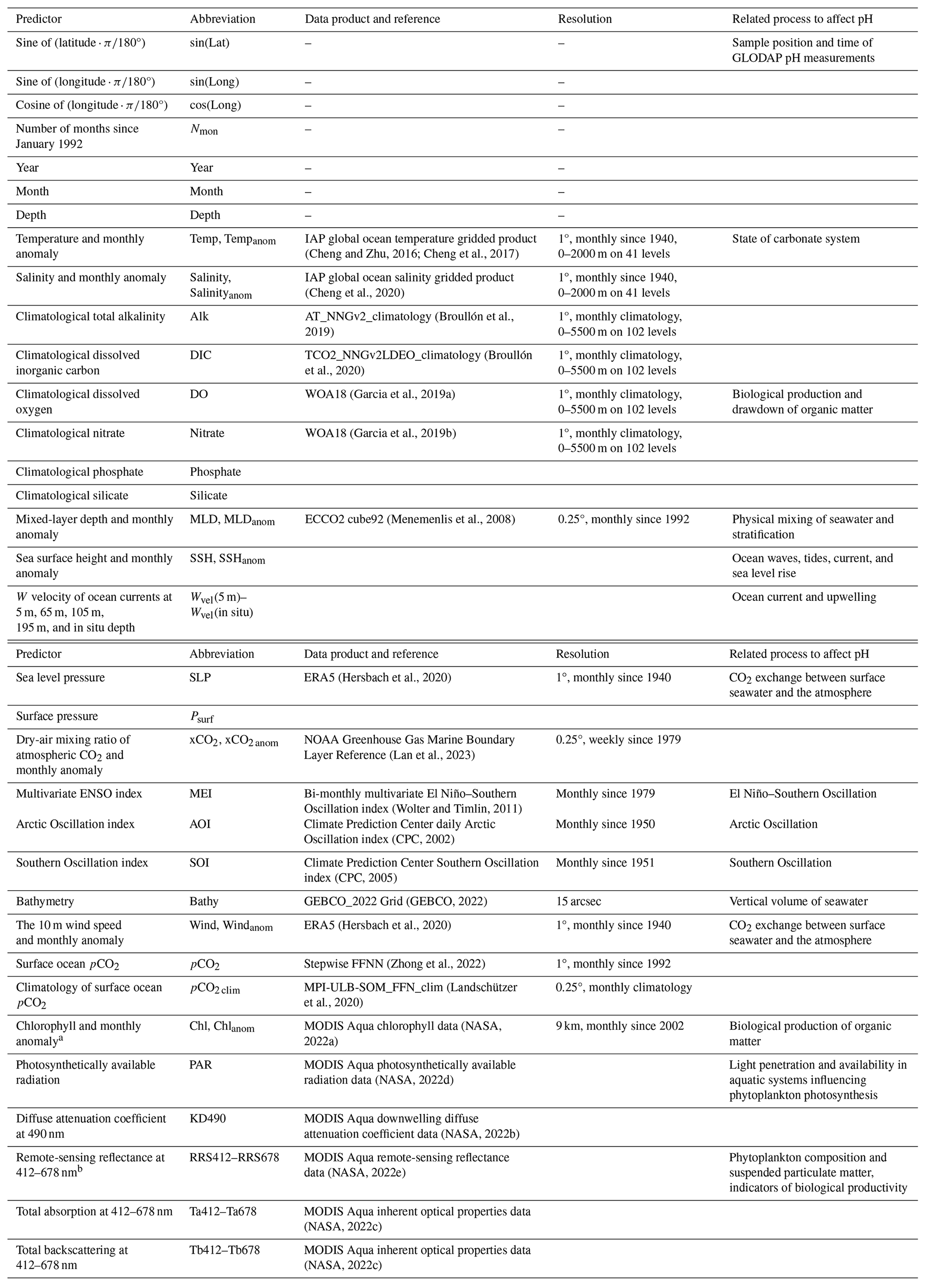
^a Products from chlorophyll to total backscattering are satellite remote-sensing products.
^b Remote-sensing reflectance, total absorption, and total backscattering both include 10 wavelengths: 412, 443, 469, 488, 531, 547, 555, 645, 667, and 678 nm. Each wavelength is regarded as one individual parameter.

On the other hand, the discrete GLODAP measurements did not match the monthly 1°×1° resolution of the pH predictor products. To be consistent with respect to the temporal and spatial resolution, the discrete GLODAP measurements were also merged into a monthly and 1°×1° resolution by averaging. The vertical layers of the temperature and salinity gridded product were used as reference standards for adjusting other collected products and constructing the pH product (Cheng and Zhu, 2016; Cheng et al., 2017, 2020). These layers covered a depth range of 0–2000 m with a total of 41 layers, including 0, 5, and 10–100 m at 10 m intervals; 120–200 m at 20 m intervals; 250–900 m at 50 m intervals; and 1000–2000 m at 100 m intervals. Subsequently, the in situ seawater measurements of pH, temperature, salinity, latitude, longitude, and depth from the GLODAP dataset were averaged monthly within the same 1°×1° grid (with the first grid centered at 89.5° S, 0.5° E) and within the same vertical layer to match the resolution of the predictor products. As a direct average was used instead of a weighted average, the average latitude, longitude, and depth values from the initial measurements within the same 1°×1° grid were then used as the new sample position for the derived monthly measurements, instead of being located at the center point of grids. The pH measurements obtained after the 1°×1° grid and monthly averaging were employed to establish a neural network model and fit a nonlinear relationship with the pH predictors.

2.2 Biogeochemical province

To identify the predictors that are most relevant to pH drivers in different regions, we divide the global ocean into distinct biogeochemical provinces using self-organizing map (SOM) neural networks. This was achieved by inputting climatological surface seawater temperature, salinity, mixed-layer depth, chlorophyll concentration, dissolved oxygen, nitrate, phosphate, silicate, and pH (Lauvset et al., 2016) into a 4×4 SOM network, resulting in the partitioning of the global ocean into 16 preliminary provinces. Subsequently, the small “island” provinces with fewer than 10 connected grids or covered by fewer than 100 GLODAP pH measurements were merged with the nearest neighboring provinces, as the pH reconstruction errors tend to be notably higher due to the extremely low number of training samples in the nonlinear relationship fitting by networks. In addition, provinces separated by continents were manually subdivided into distinct provinces, such as the province spanning the North Pacific and the North Atlantic. As a result, the global ocean was divided into 14 biogeochemical provinces, as shown in Fig. 1. The boundary of SOM provinces was treated with a cross-boundary method to relieve the discontinuity in the spatial distribution near the SOM boundaries (Zhong et al., 2022). Due to the much more dynamic variation in coastal seawater pH, the global coastal areas have higher reconstruction errors than the open oceans. In this study, we removed all coastal areas with bathymetry shallower than 200 m. Furthermore, because the drivers of seawater pH near the surface are different for deeper waters, the ocean area was divided into two layers: the mixed layer (ranging from 0 m to the mixed-layer depth) and the intermediate layer (ranging from the mixed-layer depth to 2000 m). Consequently, the gridded product construction in each province was carried out separately for the two layers. Application of the SOM method can effectively reduce regional reconstruction errors, but it also generates discontinuity problems near the boundary. Therefore, a cross-boundary method was used to improve the FFNN performance near the SOM and vertical boundary (Zhong et al., 2022). The spatial scale of training samples in each SOM province was expand out of the boundary for 10 grids and out of the vertical boundary for two layers (Fig. 2). By increasing the additional training sample outside of the SOM province and vertical layer boundary, the cross-boundary method can effectively reduce the appearance of disconnectivity near boundaries (Figs. S1 and S2 in the Supplement).

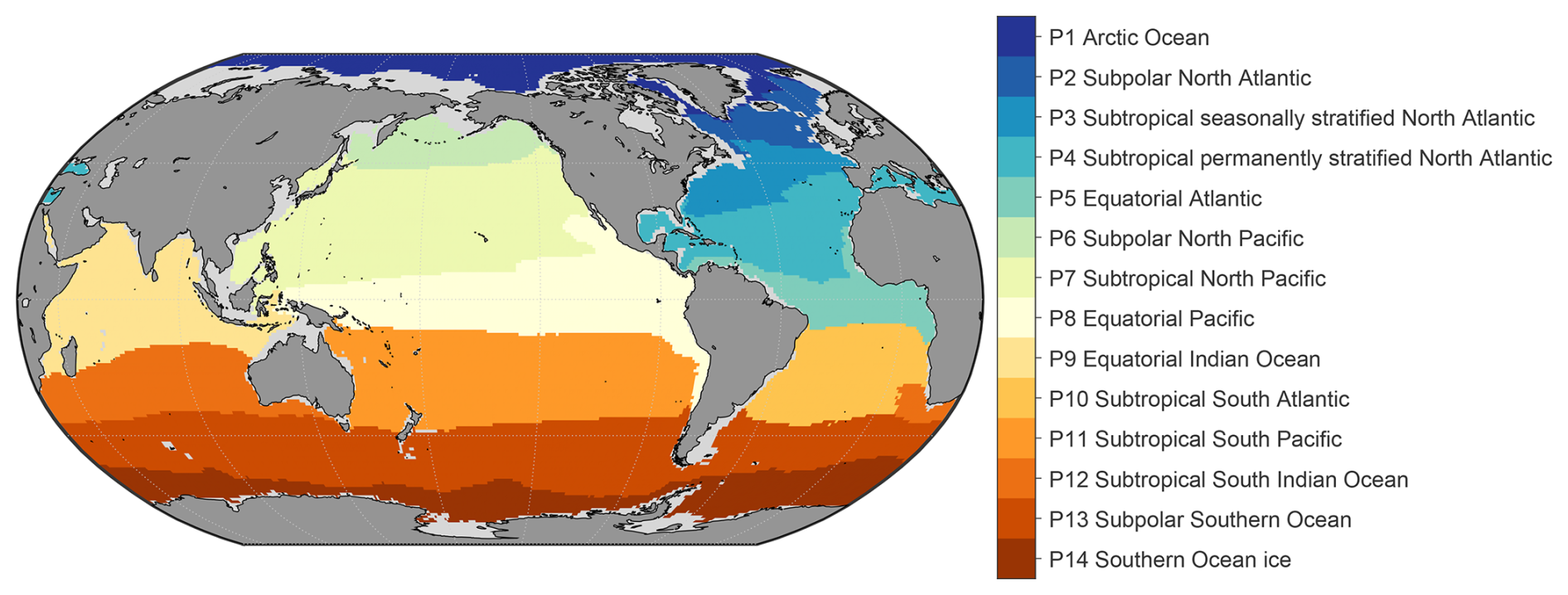
Figure 1 Map of the biogeochemical province.

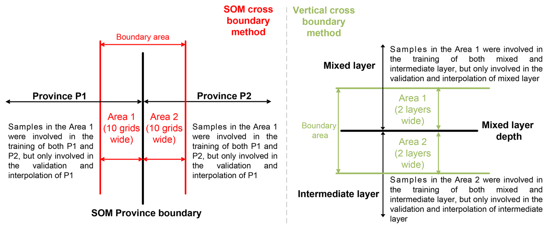
Figure 2 Cross-boundary method for better connectivity near the SOM boundary and vertical boundary.

2.3 The pH product construction

A feedforward neural network (FFNN) with a single hidden layer was applied to fit the nonlinear relationship between seawater pH and its predictors to perform spatial interpolation and construct the gridded product:

$$\begin{array}{}\text{(1)}& \text{pH}=f({\text{Predictors}}_{\mathrm{1}},{\text{Predictors}}_{\mathrm{2}},\mathrm{\dots },{\text{Predictors}}_N),\end{array}$$

where f is a nonlinear function built by the FFNN, and predictors related to chemical, physical, and biological properties were selected from the products in Table 1. Considering the regional difference in pH variability and its drivers, identifying the combination of most relevant predictors in each region was a critical precondition. Thus, the entire product construction method includes the following two steps (Fig. 3):

1. First, we undertook the selection of the seawater pH predictors in each province using the stepwise FFNN algorithm (referred as “(1) Stepwise FFNN” in Fig. 3). All of the collected products were input into the stepwise FFNN algorithm to identify the predictors that yielded the lowest reconstruction errors for seawater pH (Zhong et al., 2022). The variation in the mean absolute error (MAE) calculated by the k-fold cross-validation method is fed back to update the input products. The input variables are selected as pH predictors one by one such that the MAE decreases the fastest. Specifically, by comparing the reconstruction errors resulting from using each collected environmental variable in Table 1 as the only predictor input to the FFNN, the variable with the lowest error is selected as the first pH predictor and removed from the environmental variables list used in the subsequent steps. Subsequently, while keeping the first predictor unchanged, reconstruction errors are compared when each remaining environmental variable is used as the second input for the FFNN. The variable with the lowest error is determined to be the second pH predictor. In the same way, new predictors are sequentially determined. This selection process continued through multiple iterations until no further reduction in the MAE was observed, regardless of whether a variable was added or removed. The variables identified in previous iterations were then output as the optimal pH predictors. As both overfitting caused by co-correlation and underfitting caused by an insufficient number of predictors result in significant increases in pH reconstruction errors, the lowest reconstruction error is considered to occur between these two states. In order to eliminate potential co-correlation and prevent overfitting, whenever a new predictor is identified, the algorithm then also tests whether the reconstruction error will decrease when each determined predictor is sequentially removed. The algorithm individually removes each previously identified predictors immediately after adding one variable as a predictor. If the error decreases after removing a previously determined predictor, this predictor is highly correlated with the other identified predictors. If a certain predictor is highly correlated with existing predictors, this predictor tends to fail to compete with other variables in the adding of predictors and is generally removed in the following removal step to reduce reconstruction errors. Therefore, most of the co-correlation among the selected predictors is removed in this stepwise FFNN selection procedure. If products with co-correlations are still selected, some products may provide important additional information in specific regions, leading to a greater reduction in reconstruction errors compared with the increase caused by overfitting. Spatial and temporal variables, such as latitude, longitude, and time, are directly related to the spatial or temporal pH patterns, rather than the factor driving pH variations. This means that these variables are often co-correlated with other input environmental variables. In some regions where the environmental variables sufficiently reflect the factors influencing pH or where spatial and temporal pH patterns are not notable, adding latitude, longitude, and time as predictors does not contribute sufficient information and cannot effectively reduce prediction errors due to the co-correlation with other predictors. In these cases, these spatial–temporal variables are not selected as predictors (Tables 2 and 3). In addition, depth is important with respect to reconstructing the vertical pH distribution. However, it was not used as a predictor in certain regions of the mixed layer due to the notable similarity between the vertical pattern of pH and particular environmental variables used as predictors, such as phosphate, nitrate, and silicate. In this case, the FFNN model learned how pH varied with depth based on the similarity of the vertical pattern between seawater pH and specific physical or biological conditions indicated by input environmental variables, and it subsequently reconstructed seawater pH values at different depths using 3D fields of these environmental variables. In each province, pH predictors were selected separately for the mixed layer (Table 2) and intermediate layer (Table 3). In certain polar areas and prior to August 2002 when satellite remote-sensing products (products from Z_eu to Tb678 in Table 1) were not available, the additional selection of predictors was carried out without the use of satellite remote-sensing products (Table S1 in the Supplement). These satellite products were not used in the intermediate layer due to low correlation with seawater pH, with no need for additional selection.

2. Second, we carried out fitting of the nonlinear relationship between the seawater pH and selected predictors (referred as “(2) FFNN” in Fig. 3). In each province, a group of FFNNs were trained separately for the mixed layer and intermediate layer to fit the nonlinear relationship, based on the predictors selected in the first step and GLODAP pH measurements. To mitigate the influence of an FFNN's initial state on reconstructed values, multiple networks with the same structure but different initial states were trained and their results were averaged (standard deviation shown in Fig. S5 in the Supplement). Subsequently, the seawater pH was calculated by inputting the product of pH predictors into the trained FFNNs. As the satellite remote-sensing products used in this work lack data during the period before August 2002 and in certain polar areas during winter, the FFNNs generated missing values in these grids when remote-sensing products were used as predictors. To address these missing values, we selected additional groups of predictors after removing remote-sensing products (Table S1) and then trained additional FFNNs to predict pH in grids with missing values. This procedure was the same as the reconstruction process in the intermediate layer, in which the remote-sensing products were also not used. Finally, the seawater pH values from all FFNNs were combined to construct the global ocean 0–2000 m seawater pH gridded product from January 1992 to December 2020 at a 1°×1° spatial resolution. The pH data prior to 1992 are unavailable, as the predictors used from the ECCO2 cube92 product (Menemenlis et al., 2008) also start from 1992. Moreover, data after 2020 are limited by the coverage of the surface ocean pCO₂ product used and will be updated in future works.

All FFNNs used in these two steps have the same structure with a single hidden layer, as using deeper structures tends to cause overfitting and increase pH reconstruction errors. The number of neurons was determined by comparing the reconstruction errors of FFNNs with different neurons based on the same training samples, testing samples, and pH predictors and then adopting the number with the lowest reconstruction error. Specifically, for the stepwise FFNN regression step, the number of neurons in the FFNNs was determined using provisional predictors from preliminary experiments with the number of neurons set to 25.

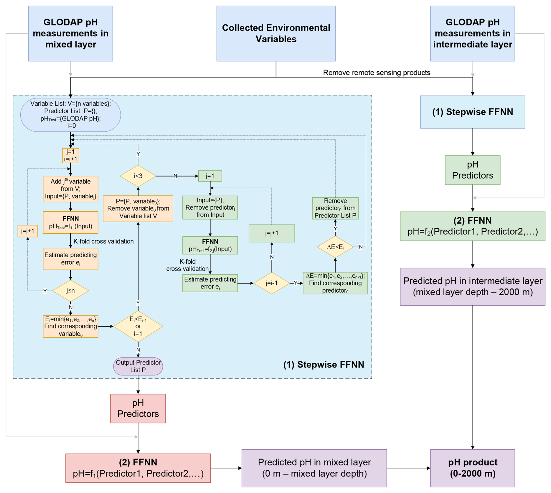
Figure 3 The procedure of pH product construction. The boxes in the flow diagram are as follows: “(1) Stepwise FFNN” denotes the algorithm for selecting predictors (Zhong et al., 2022); “(2) FFNN” represents the fitting of the nonlinear relationship between seawater pH and its predictors; “Collected Environmental Variables” represents the collected products listed in Table 1; and “pH predictors” represents the selected most informative variables listed in Tables 2 and 3. Remote-sensing products are variables from chlorophyll to total backscattering in Table 1. The mixed layer is from 0 m to the mixed-layer depth, whereas the intermediate layer is from the mixed-layer depth to 2000 m.

Table 2 Predictors selected by the stepwise FFNN algorithm in the mixed layer.

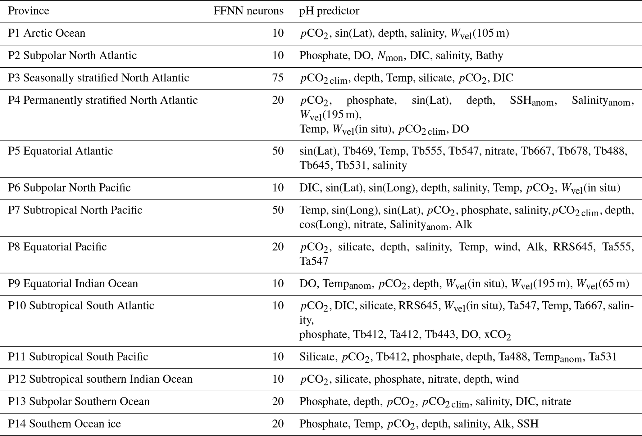
The predictors are arranged in order of relative importance, with the variables listed at the front of each province being more effective with respect to reducing reconstruction errors when used as pH predictors.

Table 3 Predictors selected by the stepwise FFNN algorithm in the intermediate layer.

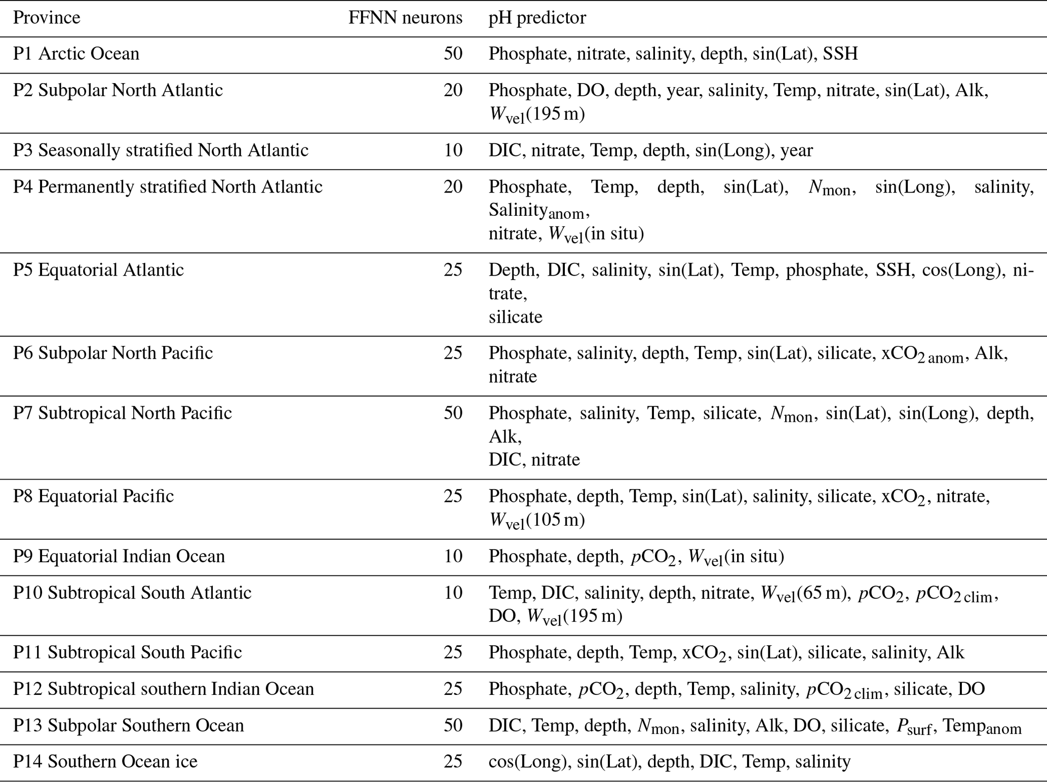
The predictors are arranged in order of relative importance, with the variables listed at the front of each province being more effective with respect to reducing reconstruction errors when used as pH predictors.

2.4 Validation and uncertainty

The reconstructed pH product was validated based on pH measurements from GLODAP and time-series stations. First, the root-mean-square error (RMSE) between the FFNN pH and GLODAP pH measurements was calculated using the k-fold cross-validation method. The GLODAP pH measurements were divided by years, and the k value was 4 to keep aside 25 % of the independent measurements for testing in each one of the four iterations. Thus, within every set of 4 consecutive years, pH measurements from 3 years were utilized for training the FFNN model, while the measurements from the remaining year were employed for testing. This approach ensured independence between the training and testing groups (Gregor et al., 2019; Zhong et al., 2022). Subsequently, the pH measurements in the testing group were compared against the FFNN pH values based on the training group. A total of four iterations were carried out, with each iteration designating different years as the testing groups, thereby ensuring that measurements from all years were set as the test group once and matched with an FFNN value. By comparing all of the FFNN pH values with GLODAP pH measurements, the RMSE values of pH and the molar hydrogen ion concentration ([H⁺]) were calculated to evaluate the performance of the FFNN model. The reconstruction of the testing group from the training group is similar to the interpolation process, wherein the FFNN is trained with existing measurements to reconstruct pH in unknown areas.

Second, the reconstructed seawater pH product was compared with independent pH measurements from the Hawaii Ocean Time-series (HOT; 22°45^′ N, 158°00^′ W; since October 1988; Dore et al., 2009), the Bermuda Atlantic Time-series Study (BAT; 31°50^′ N, 64°10^′ W; since October 1988; Bates, 2007; Bates and Johnson, 2020), and the European Station for Time-Series in the Ocean of the Canary Islands (ESTOC; 29°10^′ N, 15°30^′ W; from 1995 to 2009; González-Dávila et al., 2010). The long-term trend was further compared with data from the Irminger Sea station (64.3° N, 28.0° W; from 1983 to 2019; Ólafsson, 2016; Ólafsdóttir et al., 2020a), the Iceland Sea station (68.0° N, 12.7° W; from 1985 to 2019; Ólafsson, 2012; Ólafsdóttir et al., 2020b), and the DYFAMED station (42.3° N, 7.5° E; from 1991 to 2017; Coppola et al., 2024). To better evaluate the performance of the FFNNs below the surface, the constructed pH product was also compared to independent delayed-mode pH-adjusted data with a quality control flag of 1 from Biogeochemical Argo (BGC-Argo) profiles from the Global Data Assembly Centre (Claustre et al., 2020; Argo, 2024). Validation based on these independent measurements from time-series stations and BGC-Argo profiles provides additional evidence of data accuracy.

A comparison between the method of training FFNNs with pH and the method of training FFNNs with [H⁺] and then converting to pH was carried out in order to validate which technique has a lower pH reconstruction error (Fig. S3 in the Supplement). In addition, to identify the difference in pH variability uncertainty hidden by the logarithm among regions with the same pH RMSEs but different pH levels, the uncertainty in the reconstructed pH values was converted from the [H⁺] RMSE, instead of directly using the pH RMSE. The pH obtained from the FFNN was first converted to [H⁺] to estimate the RMSE. Subsequently, the pH values were shown as pH₀±σ at each given pH₀ value, and the local uncertainty (σ) stemming from the FFNN reconstruction errors was calculated as follows:

$$\begin{array}{}\text{(2)}& \mathit{\sigma }=-{\log }_{\mathrm{10}}\left({\mathrm{10}}^{-{\text{pH}}_{\mathrm{0}}}-{\text{RMSE}}_{\left[{\mathrm{H}}^{+}\right]}\right)-{\text{pH}}_{\mathrm{0}},\end{array}$$

where ${\text{RMSE}}_{\left[{\mathrm{H}}^{+}\right]}$ is the RMSE of [H⁺] converted from the FFNN pH in each layer of all 14 biogeochemical provinces and pH₀ is the local FFNN-predicted pH value. The σ calculated using this method is simultaneously related to the pH reconstruction error and the local pH level that serves to convert the overall province FFNN error into local errors and better distinguishes the differences in uncertainty across different regions. The uncertainty in the products used as pH predictors is one ineluctable source of the pH reconstruction errors of the FFNN model. However, the direct estimation of pH uncertainty by summing the uncertainty of each product used is not feasible. Combining the inherent uncertainties of different predictor products via error propagation relies on the partial derivatives of pH to each predictor, but the nonlinear relationships established by the FFNN do not have a specific formula, leading to the difficulty in calculating the partial derivatives. Therefore, the local uncertainty in our pH product was directly estimated from the regional FFNN pH reconstruction errors and the local pH values following formula (2), instead of synthesizing the inherent uncertainty in each predictor product used via the propagation of errors. The inherent uncertainty and construction method of the predictor products are described in the Sect. S1 in the Supplement.

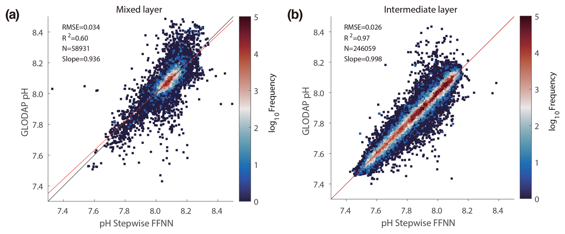
Figure 4 Comparison between FFNN pH and GLODAP pH measurements. (a) The mixed layer is from the surface to the mixed-layer depth. (b) The intermediate layer is from the mixed-layer depth to 2000 m. The black line denotes the y=x line, whereas the red line is the linear regression between the GLODAP pH and stepwise FFNN pH (Lauvset et al., 2024). Slope denotes the slope of the linear regression.

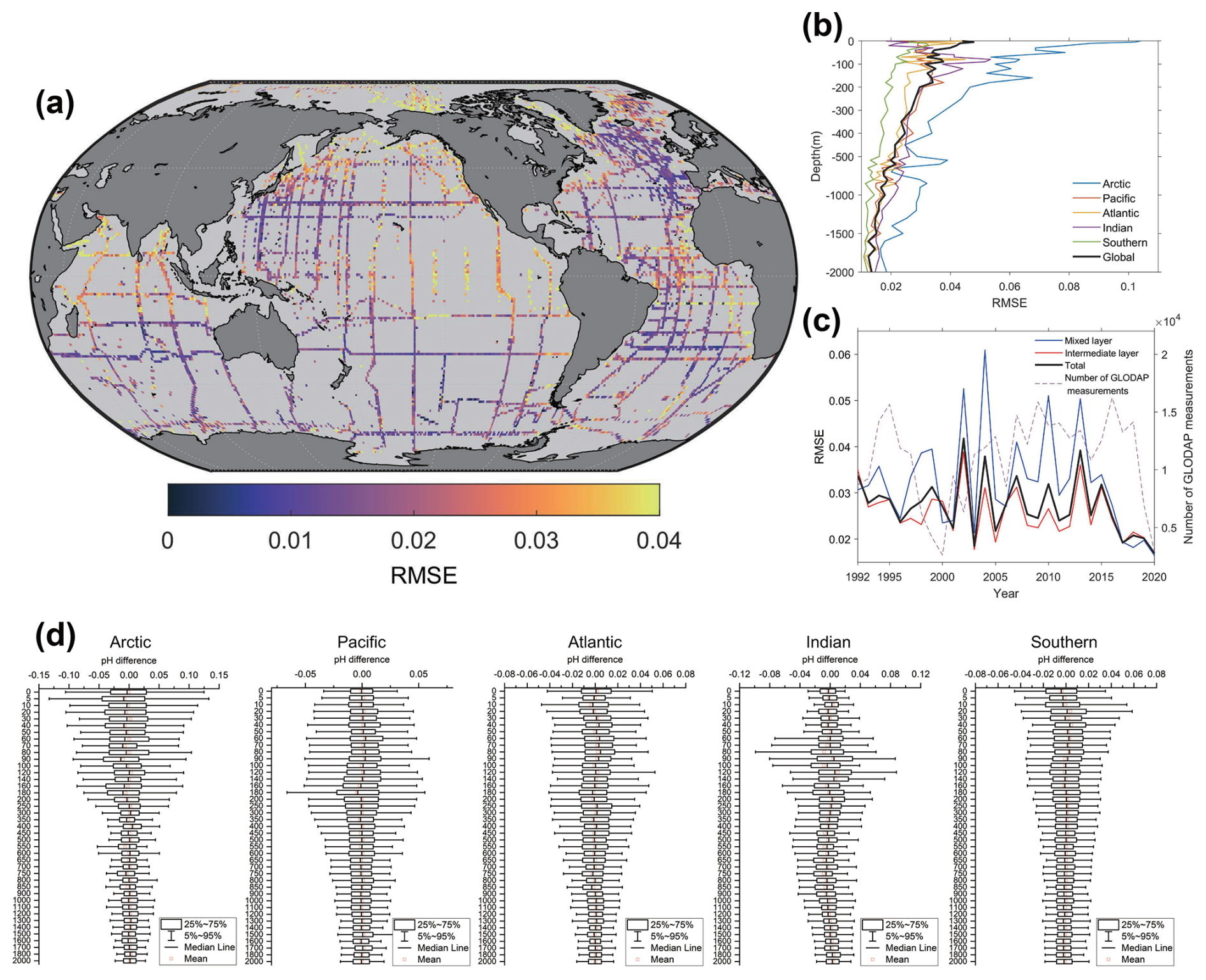
Figure 5 Distribution of the RMSE between the FFNN pH values and GLODAP pH measurements. (a) The global spatial distribution of the RMSE between the FFNN pH and GLODAP pH measurements at 0–2000 m (Lauvset et al., 2024). (b) The basin average RMSE at different depths. (c) The temporal distribution of the global RMSE. (d) The statistical distribution of the pH difference between reconstructed pH values and GLODAP pH measurements in each basin.

3 Results and discussion

3.1 Validation of the algorithm

3.1.1 Validation based on GLODAP and time-series measurements

Compared with the GLODAP dataset, most reconstructed values of the stepwise FFNN are close to the GLODAP pH measurements, concentrated around the y=x line (Fig. 4). Only a few samples differ notably between the pH measurements and the reconstructed values, with an RMSE of 0.028 in the global ocean between 0 and 2000 m. Better performance of the FFNN was found in the intermediate layer, with the testing samples being more concentrated on the y=x line. The RMSE in the mixed layer was 0.034, whereas it was higher than 0.026 in the intermediate layer. The minor difference between the reconstructed value and the pH measurements and the R² of 0.97 in the intermediate layer may be caused by less pH variability at depth and a better model fit with a broader pH value range.

The RMSE values between the FFNN pH and GLODAP pH measurements for most grids were lower than 0.03 (Fig. 5a). The performance of the FFNN was relatively better in the temperate oceans, with an RMSE of less than 0.02 for some temperate grids. However, a relatively higher RMSE was found in the equatorial and polar oceans, especially in the eastern equatorial Pacific, the near-polar North Pacific, and the northwestern Indian Ocean. The RMSE was relatively lower in regions with concentrated GLODAP measurements, such as the near-polar North Atlantic, the South Atlantic, and the southern Indian Ocean.

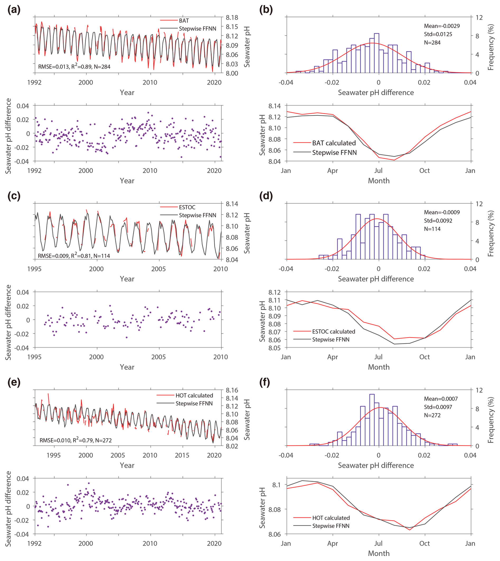
Figure 6 A comparison between the FFNN pH and time-series measurements showing the pH value, pH difference, and its distribution and the pH seasonal variability in the FFNN result and time-series measurements at (a, b) the BAT station, (c, d) the ESTOC station, and (e, f) the HOT station.

Due to the higher seasonal and interannual variability in seawater pH near the surface ocean, the RMSE decreases with depth in all basins (Fig. 5b). For the surface ocean, the RMSE between the FFNN pH and the GLODAP pH measurements was 0.044. The RMSE fluctuates between 0.032 and 0.048 at the subsurface (0–200 m). The RMSE between the FFNN pH and the GLODAP pH measurements decreased rapidly from 200 m depth. In the global ocean at 1500–2000 m depth, the global RMSE was lower than 0.015. However, the global ocean RMSE at 2000 m depth was 0.013, with a higher RMSE in the Arctic Ocean and a lower RMSE in the Southern Ocean. The vertical distribution of the RMSE and the statistical distribution of the pH difference in different basins suggest a relatively higher reconstruction error in the mixed layer than in the intermediate layer (Fig. 5d). The vertical difference in the RMSE between the mixed layer and intermediate layer was most notable in the Arctic and Indian oceans, where the RMSE values at different depths were also higher than the other basins. The RMSE in the surface Arctic Ocean was higher than 0.10 and decreased rapidly to 0.025 by 450 m depth. On the contrary, the RMSE of the surface Indian Ocean was 0.018, but it increased to 0.053 by 80 m depth and then decreased continuously with depth. The high RMSE of subsurface oceans is because there are almost no GLODAP pH measurements for the entire Indian Ocean at 50–150 m depth. The RMSE in different years also suggested a notable influence of the number of pH measurements on the FFNN reconstruction errors. The RMSE in the early years was relatively higher than in recent years, while the number of GLODAP measurements increased over the years (Fig. 5c).

The stepwise FFNN pH product showed variability in the seawater pH close to the independent time-series observations of the surface ocean from the HOT, ESTOC, and BAT stations (Fig. 6). At the BAT station, the RMSE between the reconstructed pH and time-series observations was 0.013. The surface seawater pH of our stepwise FFNN product decreased by $\mathrm{0.0017}\pm \mathrm{0.0007}{\mathrm{yr}}^{-\mathrm{1}}$ on average over the past 3 decades at the BAT station, close to the $-\mathrm{0.0018}\pm \mathrm{0.0001}{\mathrm{yr}}^{-\mathrm{1}}$ of BAT time-series observations during the same period (Bates and Johnson, 2020). At the ESTOC station, the stepwise FFNN product and time-series observations were also very consistent, with an RMSE of 0.009 and a similar long-term trend (González-Dávila et al., 2010). The RMSE between the stepwise FFNN product and the HOT time-series observations was also 0.010, and the long-term trend in the stepwise FFNN pH product was $\mathrm{0.0018}\pm \mathrm{0.0004}{\mathrm{yr}}^{-\mathrm{1}}$, consistent with the HOT time-series observations. Although the stepwise FFNN product suggested a smaller seasonal change scale than the time-series observations at the BAT station, the seasonal patterns of surface seawater pH were consistent between the stepwise FFNN product and time-series observations at all three stations. The extreme values not reconstructed by the FFNN are mainly observed at the BAT station near 2010, at the HOT station near 2000 during La Niña events, and at the HOT station before 2000 during El Niño events. In contrast, the extreme values not reconstructed by the FFNN are less common for the ESTOC station, where the surface pH did not notably fluctuate during El Niño or La Niña events. It can be inferred that the extreme values not reconstructed by the FFNN may be due to its underestimation of the impact of El Niño or La Niña events on the pH of certain temperate areas. Compared to previous surface ocean seawater pH products, which were derived from reconstructed DIC, TA, or pCO₂ products, the stepwise FFNN product was consistent with the pH trend from the majority of time-series stations (Table 4). The long-term pH trend in our product at the ESTOC station was slower than other gridded products, but the result is still close to the $-\mathrm{0.0016}\pm \mathrm{0.0001}{\mathrm{yr}}^{-\mathrm{1}}$ of real observations. At the Irminger Sea station, the FFNN pH trend was notably faster compared with the results of time-series observations. However, differences in the pH trend among pH products were most remarkable at this station. On a global scale, the pH trend in our FFNN product is $-\mathrm{0.0015}\pm \mathrm{0.0002}$ over the period from 1992 to 2020. There is no significant difference between our FFNN product, the CMEMS product, and the Copernicus product considering the current uncertainty.

Table 4 Comparison of the surface acidification rate with a previous product for different time-series stations and at a global scale.

The trends from different products for comparison were recalculated based on data during same period noted in the second column. The stepwise FFNN product was reconstructed from pH measurements with a 1°×1° and monthly resolution from 1992 to 2020, covering the global open ocean from 0 to 2000 m. The JMA product was reconstructed from DIC and Alk with 1° and monthly resolutions from 1990 to 2022, covering the global surface ocean except a portion of the Arctic. The CMEMS product was reconstructed from pCO₂ and Alk with 1° or 0.25° resolutions and a monthly resolution from 1985 to 2021, covering the global surface ocean except a portion of the Arctic. The OS-ETHZ product was reconstructed from pCO₂ and Alk with 1° and monthly resolutions from 1982 to 2022, covering the global surface ocean except the Arctic. The Copernicus product is a mean seawater pH time series and trend from 1985 to 2021 from multi-observation reprocessing.

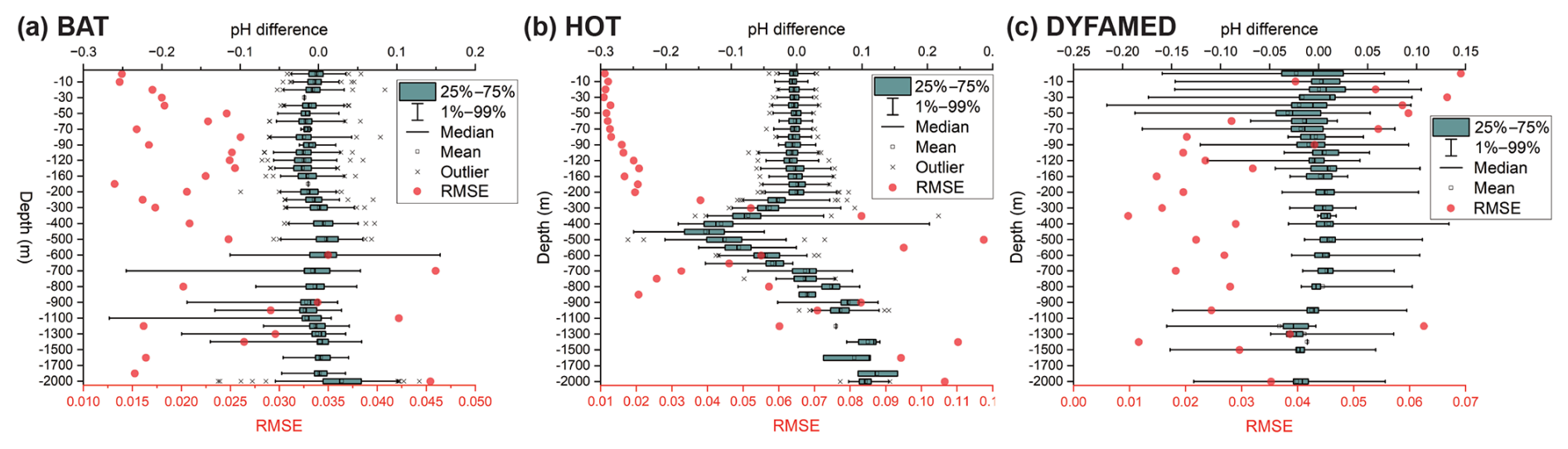
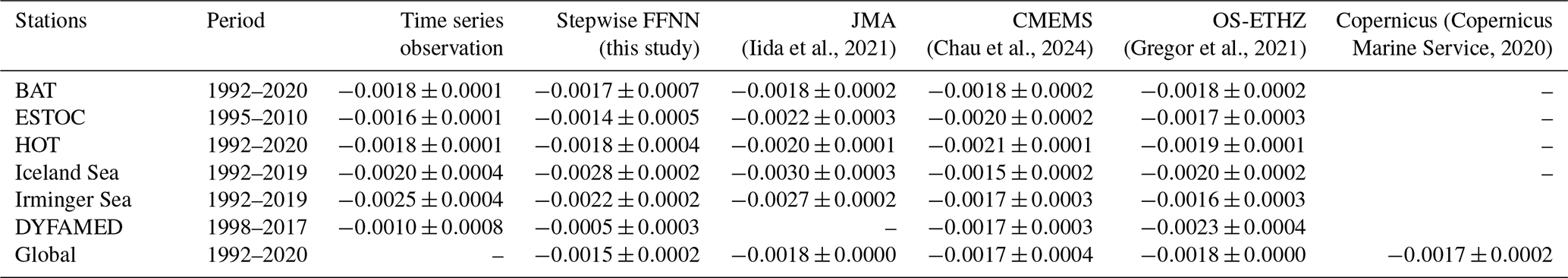
Figure 7 The RMSE and pH difference between the FFNN pH and time-series observations at different depths for the (a) BAT station (31°50^′ N, 64°10^′ W) based on data from 1992 to 2020, (b) the HOT station (22°45^′ N, 158°00^′ W) based on data from 1992 to 2020, and (c) the DYFAMED station (42.3° N, 7.5° E) based on data from 1998 to 2017.

Compared with the time-series data below the surface, the FFNN pH was close to the pH observations in the upper few hundred meters at the BAT and HOT station (Fig. 7). However, higher RMSE values and larger pH difference ranges were observed between 500 and 1500 m at the BAT station and below 300 m at the HOT station. This may be due to the sparser GLODAP observations used to train the FFNN model in these areas. Additionally, as depth is used as a pH predictor in the validation based on the GLODAP dataset, the FFNN pH values used for validation were outputted at the same depth as the GLODAP observations. When comparing the FFNN pH with independent time-series observations, differences in depth between the pH product and the observations can amplify the calculated pH difference and RMSE. For example, the FFNN pH product was reconstructed at bottom depths of 1800 and 2000 m. Thus, if a time-series observation was at 1910 m depth, it would be compared with the FFNN pH value at 2000 m in the independent validation. This depth difference significantly increases the pH error in the validation based on independent data. Despite higher RMSEs at certain depths, the RMSE at most depths in the deep areas of BAT station and DYFAMED station was below 0.03, indicating that the notable deviations may only occur at the local scale.

3.1.2 Validation based on BGC-Argo float pH measurements

Comparison with time-series observations in deeper oceans suggested that the distribution of the pH reconstruction errors with depth varies notably across different stations. To better assess the performance of the FFNN in the reconstruction of pH at different depths, the FFNN-reconstructed pH was further evaluated via comparison with independent BGC-Argo delayed-mode pH-adjusted data with a quality control flag of 1 at various depths (Argo, 2024), with the spatial positions shown in Fig. S6 in the Supplement. In contrast to the validation results based on the GLODAP dataset, the RMSE between the FFNN pH and BGC-Argo pH data in the intermediate layer is 0.051, whereas it is higher than 0.035 in the mixed layer (Fig. 8a and b). In both the mixed layer and intermediate layer, most samples were evenly distributed around the y=x line. However, in the intermediate layer, some samples were slightly offset and distributed below the y=x line, which may be the main reason for the notably higher RMSE between the FFNN pH and BGC-Argo pH data in the intermediate layer. Overall, there is a good linear correlation between the FFNN-reconstructed pH and independent BGC-Argo pH data, with R² values of 0.73 and 0.84 in the mixed layer and intermediate layer, respectively.

Figure 8 The difference between the FFNN pH and BGC-Argo float pH. (a) Comparison between the FFNN pH and BGC-Argo float pH in the mixed layer. (b) Comparison between the FFNN pH and BGC-Argo float pH in the intermediate layer. (c) Statistical distribution of the pH difference (FFNN pH minus BGC-Argo float pH) at different depth levels. FFNN pH denotes pH data reconstructed in this work, while BGC-Argo pH denotes BGC-Argo pH data from the French Coriolis Global Data Assembly Centre (Argo, 2024).

The distribution of pH differences between the FFNN pH and BGC-Argo pH data at different depths reveals relatively smaller biases above 500 m (Fig. 8c). However, below 500 m, the bias between the FFNN pH and BGC-Argo pH data increases with depth and is the most remarkable at 2000 m. Comparing the pH biases calculated based on the BGC-Argo dataset and the GLODAP dataset, it is evident that only the bias between FFNN pH and BGC-Argo pH data tends to be more notable in deep areas except the Pacific Ocean (Table 5). In contrast, greater biases between the FFNN pH and GLODAP pH occur mainly in the surface layer, with the largest biases in the surface Indian Ocean. This disparity in distribution patterns between biases based on the BGC-Argo dataset and the GLODAP dataset is most remarkable in the Southern Ocean. Below 1000 m depth, the bias between the FFNN pH and GLODAP pH is near zero, whereas the bias between FFNN pH and BGC-Argo pH data is up to a range of 0.040–0.068 between 1000 m and 2000 m. These differences between the FFNN pH and BGC-Argo pH data are primarily attributed to the discrepancies between the GLODAP dataset and the BGC-Argo dataset in the deep ocean, as our product was based on the GLODAP dataset and small biases in GLODAP pH were observed in the deep ocean.

Table 5 The pH bias by area and depth computed with the BGC-Argo and GLODAP dataset.

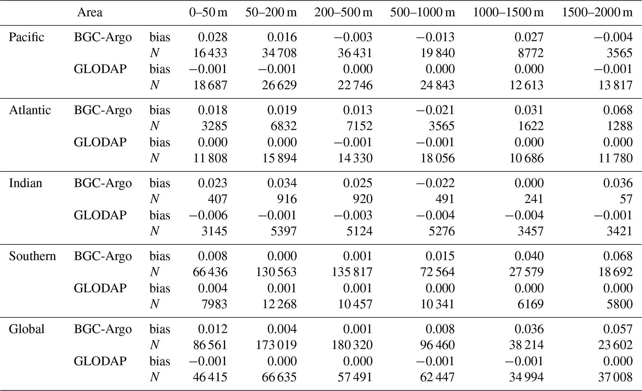
Note that N is the number of BGC-Argo or GLODAP samples used to compute the biases.

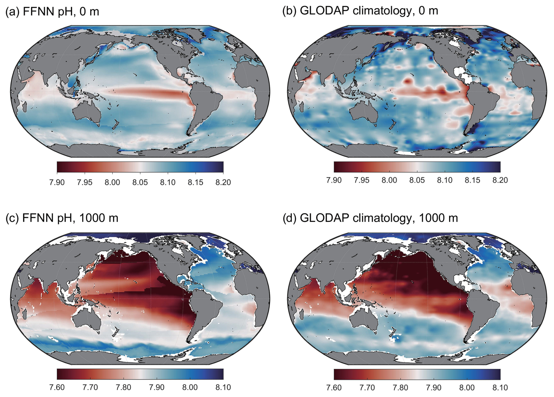
Figure 9 The average pH distribution from the FFNN pH product and GLODAP climatology normalized to the year 2002. The GLODAP climatology data are from Lauvset et al. (2016).

3.2 Gridded pH product

3.2.1 Spatial pH distribution

The spatial distribution of the long-term average seawater pH in the stepwise FFNN product suggests the lowest surface seawater pH in the equatorial Pacific, with an average value near 8.00 (Fig. 9a), which is in good agreement with the surface seawater pH range of 7.91–8.12 observed in the equatorial Pacific in recent decades (Sutton et al., 2014). The upwelling transporting the deep water with high dissolved inorganic carbon and low pH to the surface was the main driver. The equatorial Indian Ocean and the equatorial Atlantic also show a low surface pH of about 8.05, consistent with the distribution patterns of the GLODAP pH climatology (Lauvset et al., 2016). The highest surface pH is found in the Atlantic sector of the Arctic Ocean, where the average surface pH was around 8.15 over the past 3 decades. Moreover, the average surface pH in temperate oceans is relatively higher, such as in the southern Indian and South Atlantic oceans. In the temperate Pacific Ocean, differences in surface pH levels were observed between the west and east in both our product and the GLODAP pH climatology, which may have been caused by the spread of eastern equatorial seawater with an extremely low pH. At the deeper depth of 1000 m, the spatial distribution pattern of the FFNN pH product is generally consistent with the GLODAP climatology, despite some existing disturbance due to bad FFNN performance along the SOM province boundary and the higher FFNN pH in the Southern Ocean.

The vertical distribution of the average pH in the proposed product showed a notable pH decrease with increasing depth in the upper 500 m of different basins (Fig. 10). The seawater pH was the lowest at nearly 500 m and rose with increasing depth at 500–2000 m in the Pacific and Atlantic oceans. The distribution pattern of the seawater pH in the Indian Ocean was similar to that in the South Pacific, with the lowest seawater pH appearing near 1000 m. The subsurface seawater with low pH in the Atlantic Ocean and Indian Ocean was mainly concentrated in the equatorial region. In contrast, subsurface seawater with low pH in the Pacific Ocean appeared in subpolar and equatorial regions. The overall distribution pattern of the reconstructed pH is in good agreement with previous research (Lauvset et al., 2016, 2020). It can be concluded that the FFNN fitted the relationship between GLODAP seawater pH and its predictors well and that the proposed pH product has good accuracy.

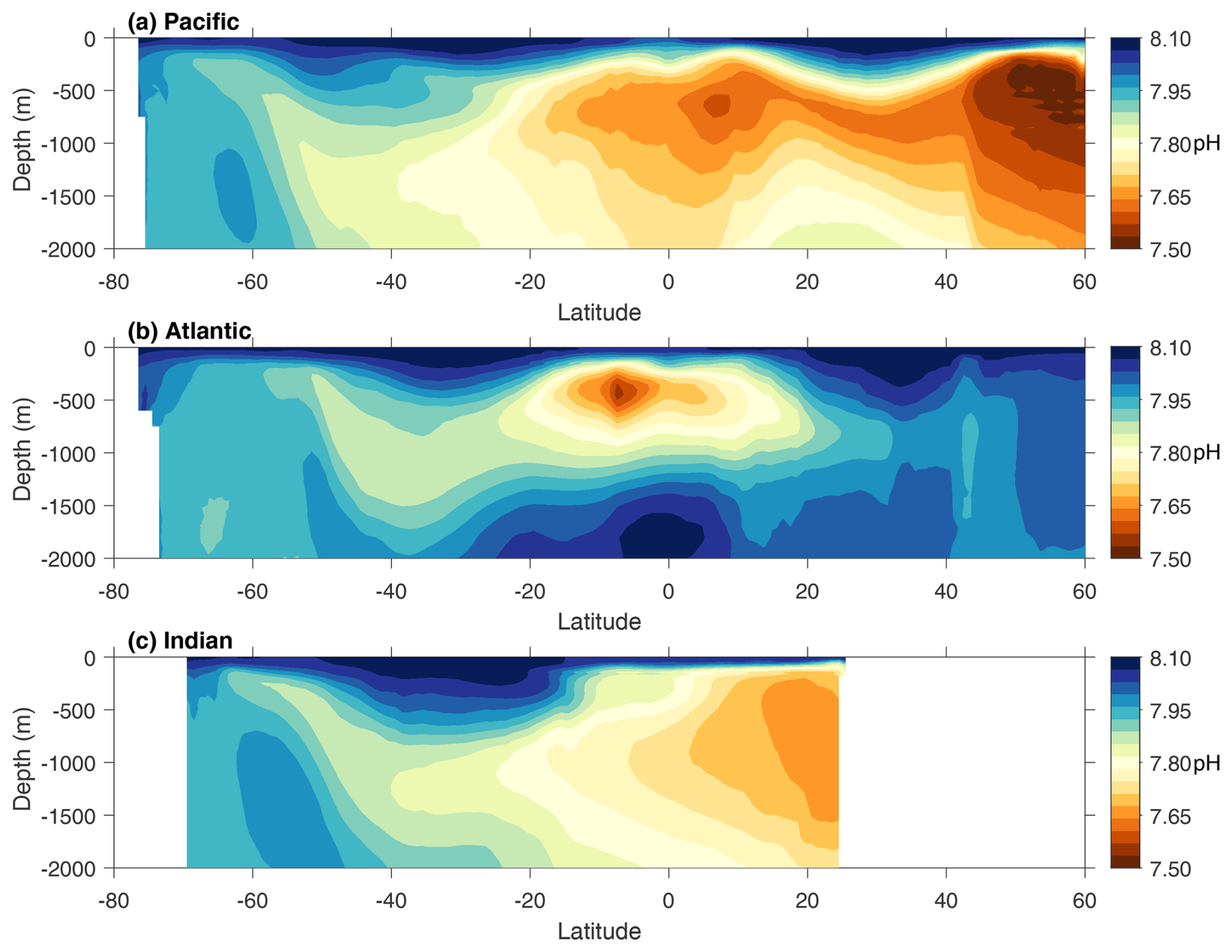
Figure 10 Climatological vertical distribution of the zonal average FFNN pH in the main basins. The pH values shown at each latitude were averaged from pH values across all longitudes within each major basin.

Based on the pH predictors selected by the stepwise FFNN algorithm, differences in the processes driving pH variability were identified between the mixed layer and the intermediate layer in most provinces. In the mixed layer, surface ocean pCO₂ was identified as the most informative predictor in many provinces, followed by temperature and the nutrient concentration. This suggests that the CO₂ exchange between the surface ocean and the atmosphere is the primary driver of pH variability, followed by biological CO₂ utilization and seasonal changes in the seawater temperature. In contrast, phosphate was identified as the most informative predictor in the intermediate layer, followed by temperature and depth. This suggests that the primary process driving pH variability is the remineralization of organic matter, converting organic carbon into inorganic forms and also releasing nitrogen and phosphorus. Given the notably smaller seasonal temperature changes in the intermediate layer compared with the mixed layer, the selection of temperature as an important pH predictor may indicate a notable influence of ocean warming on seawater pH variability. Additionally, depth was also selected as an important predictor in the intermediate layer. The observed pattern of seawater pH decreasing with increasing depth in most provinces, as suggested by the constructed pH product, may be the main reason.

Figure 11 Uncertainty in the FFNN pH product in the main basins.

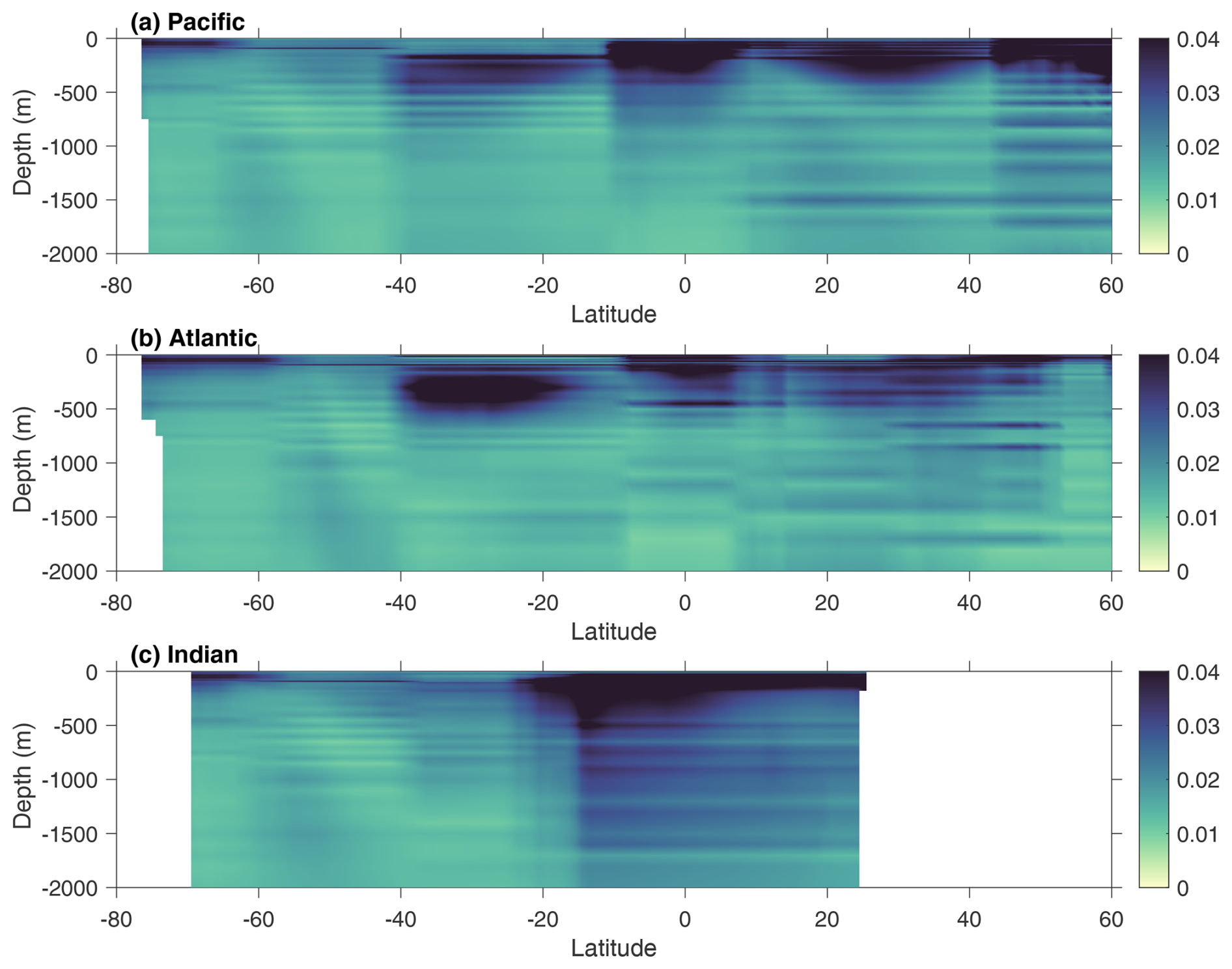
3.2.2 Uncertainty

As described in Sect. 2, the FFNN pH was converted to [H⁺] to calculate the regional RMSE of [H⁺] between the FFNN results and GLODAP measurements, and the RMSE of [H⁺] in each SOM province was then used to calculate the pH product uncertainty caused by the construction algorithm (Eq. 2). Due to higher reconstruction errors, the pH product uncertainty is relatively higher near the surface (Fig. 11). The uncertainty is generally lower than 0.02 at depths from 500 to 2000 m, except for some regions near the SOM province and vertical boundary. Although we have used a cross-boundary method to improve the FFNN performance near the SOM and vertical boundary, there are still some discontinuity problems and relatively higher uncertainty. This is because the pH values on two sides of the SOM boundary were reconstructed from two different FFNN models that were trained with different samples and used different predictors. Thus, if one of the FFNN models experiences worse performance due to insufficient training samples or predictors, the pH values on two sides of the SOM boundary will still differ notably, resulting in discontinuity along the boundary. Therefore, regional-scale analysis based on pH values near SOM boundaries should be carried out more cautiously when using our product. In addition, the equatorial and polar regions show an uncertainty higher than 0.04. This is because the FFNN performance tends to be worse in regions with the highest and lowest pH levels, compared with regions in which pH values are near average. Especially in the Arctic Ocean, the pH measurements are much sparser, leading to the highest reconstruction error and pH uncertainty. Therefore, the proposed pH product should be cautiously used in regional analysis near the boundaries or equatorial and polar regions.

4 Data availability

The materials used in this research, including the gridded seawater pH product (NetCDF files for all individual years), the MATLAB code for reconstruction and validation, and other materials (available as .m or .mat files), are available from the Marine Science Data Center of the Chinese Academy of Sciences at https://doi.org/10.12157/IOCAS.20230720.001 (Zhong et al., 2023). The pH measurements used are available from GLODAP (https://glodap.info/index.php/merged-and-adjusted-data-product-v2-2023/, last access: 5 February 2024, Lauvset et al., 2024). Data products used for predictors are available from the references listed in Table 1.

5 Conclusions

Quantifying the global seawater pH variability is important for understanding the future responses of oceans with respect to the uptake of anthropogenic CO₂. A 4D global seawater pH product covering depths from the surface to 2000 m and the years from 1992 to 2020 was reconstructed in this work. This product serves as a reference for guiding acidification surveys by providing a general understanding of acidification process at different depths at the basin scale and indicating areas with potential fast or slow acidification rates. Additionally, the pH product provides insights into acidification research and can be used to analyze the influence of specific ocean processes on acidification rates and the broader impacts of acidification on a large scale when direct observations are unavailable. However, caution should be exercised when using this product for regional analyses at a small spatial scale. The analysis of the pH RMSE and uncertainty suggested that the proposed pH product remains limited in equatorial and polar regions and along the SOM boundary lines. This limitation was caused by sparse measurements and method disadvantages, which can be mitigated via future improvement works. Potential improvement may be achieved by increasing the number of predictor products to capture the pH drivers, testing more machine learning algorithms, and accumulating more seawater pH observations. Furthermore, the method used to reconstruct the pH product can be applied in the reconstruction of global fields of other ocean chemical variables, such as nutrients, particulate organic carbon, and dissolved inorganic carbon. The global field of these variables may further improve the pH product accuracy, as climatological products of these variables were used as pH predictors and lacked information on interannual variability. Overall, decreasing seawater pH will influence the metabolism of marine organisms and result in notable changes in the marine ecosystem. Discrete observations may be insufficient to support research on large scales. With the machine learning method in this work, discrete pH measurements were mapped to global gridded fields to fill the unsampled areas. Our product can be used for the analysis of seasonal to decadal and regional to global pH variability, to break through the limitation of discrete observations.