the Creative Commons Attribution 4.0 License.
the Creative Commons Attribution 4.0 License.
 | 06 May 2024
The Total Carbon Column Observing Network's GGG2020 data version
Joshua L. Laughner
Geoffrey C. Toon
Joseph Mendonca
Christof Petri
Sébastien Roche
Debra Wunch
Jean-Francois Blavier
David W. T. Griffith
Pauli Heikkinen
Ralph F. Keeling
Matthäus Kiel
Rigel Kivi
Coleen M. Roehl
Britton B. Stephens
Bianca C. Baier
Huilin Chen
Yonghoon Choi
Nicholas M. Deutscher
Joshua P. DiGangi
Jochen Gross
Benedikt Herkommer
Pascal Jeseck
Thomas Laemmel
Erin McGee
Kathryn McKain
John Miller
Isamu Morino
Justus Notholt
Hirofumi Ohyama
David F. Pollard
Markus Rettinger
Haris Riris
Constantina Rousogenous
Mahesh Kumar Sha
Kei Shiomi
Kimberly Strong
Ralf Sussmann
Voltaire A. Velazco
Steven C. Wofsy
Minqiang Zhou
Paul O. Wennberg
The Total Carbon Column Observing Network (TCCON) measures column-average mole fractions of several greenhouse gases (GHGs), beginning in 2004, from over 30 current or past measurement sites around the world using solar absorption spectroscopy in the near-infrared (near-IR) region. TCCON GHG data have been used extensively for multiple purposes, including in studies of the carbon cycle and anthropogenic emissions, as well as to validate and improve observations from space-based sensors. Here, we describe an update to the retrieval algorithm used to process the TCCON near-IR solar spectra and to generate the associated data products. This version, called GGG2020, was initially released in April 2022. It includes updates and improvements to all steps of the retrieval, including but not limited to the conversion of the original interferograms into spectra, the spectroscopic information used in the column retrieval, post hoc air mass dependence correction, and scaling to align with the calibration scales of in situ GHG measurements.
All TCCON data are available through https://tccondata.org/ (last access: 22 April 2024) and are hosted on CaltechDATA (https://data.caltech.edu/, last access: 22 April 2024). Each TCCON site has a unique DOI for its data record. An archive of all the sites' data is also available with the DOI https://doi.org/10.14291/TCCON.GGG2020 (Total Carbon Column Observing Network (TCCON) Team, 2022). The hosted files are updated approximately monthly, and TCCON sites are required to deliver data to the archive no later than 1 year after acquisition. Full details of data locations are provided in the “Code and data availability” section.
- Article
(16836 KB) - Full-text XML
- BibTeX
- EndNote


The Total Carbon Column Observing Network (TCCON) is a network of nearly 30 ground-based, solar-viewing, Fourier transform infrared (FTIR) spectrometers that report observations of column-average mole fractions of CO2, CH4, N2O, CO, HF, H2O, and HDO in the atmosphere. The first two TCCON stations were established in 2004, with additional stations joining over the following years. As of July 2023, 30 sites exist. In that time, TCCON data have been used to estimate or evaluate carbon fluxes (e.g., Keppel-Aleks et al., 2012; Peiro et al., 2022), for satellite validation (e.g., Wunch et al., 2017; Chen et al., 2022; Lorente et al., 2022), for model verification (e.g., Byrne et al., 2023), and for other purposes.
The need for updates to the retrieval algorithm used by TCCON has been largely driven by the need for increasingly high accuracy and precision in total column greenhouse gas (GHG) data for carbon cycle science and satellite validation. GHG measurements require high precision to distinguish signals from anthropogenic, terrestrial, or oceanic processes from the background mixing ratios. The 2018 National Academies decadal strategy recommends that random and systematic errors for CO2 be less than 1 and 0.2 ppm (∼0.25 % and ∼0.05 %), respectively, and likewise less than 6 and 2.5 ppb (∼0.3 % and ∼0.1 %), respectively, for CH4 (National Academies of Sciences, Engineering, and Medicine, 2018, Table B.1, question C-3, p. 601). Future space-based CO2-observing missions are striving for even greater precision; for example, CO2M has a stated goal of 0.7 ppm precision and <0.5 ppm systematic error in (ESA, 2020). The increasingly stringent precision requirements for carbon cycle science and satellite validation demand that ground-based networks, such as TCCON, continue to refine their data to support these requirements.
A second factor driving improvements in the retrieval is the emergence of portable, low-resolution, solar-viewing, FTIR instruments such as EM27/SUNs. These instruments can be deployed to areas that cannot support a full TCCON site and are also affordable enough to be deployed in greater density around locations of interest (e.g., cities). This capability complements the higher-precision and higher-accuracy data produced by TCCON. To facilitate comparisons between TCCON and EM27/SUN data, it is beneficial to use the same retrieval for both. Improvements to the handling of EM27/SUN interferograms (Sect. 4.3) have been added.
TCCON instruments record interferograms of direct-sun measurements in the near-IR wavelengths. These interferograms are transformed into spectra from which the final column-average mole fractions (henceforth denoted as Xgas, e.g., ) are derived using the retrieval software GGG.1 Major versions of GGG are identified by the year of development. The previous version used to generate public TCCON data was GGG2014 and is described in Wunch et al. (2015) (see also Wunch et al., 2011, 2010). GGG2020 is the first major update applied to TCCON public data since GGG2014. The primary goal of this paper is to describe the changes in GGG2020 compared to GGG2014.
GGG retrieves trace gas column amounts by iteratively scaling an a priori trace gas vertical profile until the best fit between a spectrum simulated from those trace gas profiles by the built-in forward model and the observed spectrum is found. This differs slightly from the Bayesian framework described in Rodgers (2000); please refer to Sect. 3.4 of Roche (2021) for a discussion of specific differences. A single gas may be fit in more than one spectral window; for example, GGG2020 produces the standard TCCON CO2 product from two separate retrievals using two spectral windows (6220 to 6260 and 6297 to 6382 cm−1). Each window is run separately and produces its own posterior scaled trace gas profile, which is separately integrated to generate a column density from each window. These column densities are combined and converted to the final Xgas value. Retrieving each window separately, rather than concatenating the spectral information, makes it simpler to handle non-contiguous windows that need different state vector elements. It also allows biases that differ between these windows to be expressed separately in the resulting output data and, if necessary, corrected separately. The output values (column densities and profile scaling factors) from different windows with similar averaging kernels for the same target gas are combined in a weighted average during post-processing.
The post-processing step includes the conversion from column densities to column-average dry mole fractions, followed by the above window-to-window averaging, an empirical air-mass-dependent correction, and a scaling correction to tie TCCON data to the relevant calibration scales. Air-mass-dependent errors can arise from, for example, errors in the relative intensities of strong and weak absorption lines for a target gas. At large solar zenith angles (SZAs), the longer light paths through the atmosphere will cause strong absorption lines to completely absorb incoming light within their core wavelengths; such lines may be referred to as “blacked out”. Blacked-out lines cannot contribute information to the retrieval; thus, the retrieval must get a greater fraction of its information from weaker lines in the spectral window or the wings of saturated lines. If there is a different bias in the forward model between the strong and weak lines, it will manifest as an error in the retrieved column amounts that varies with SZA and is symmetric about solar noon. Once the magnitude of this error is derived (Sect. 8.1), a post-processing correction is applied to mitigate it.
Applying a scaling factor to tie to the in situ calibration scales is necessary because the spectroscopic parameters used in the forward model are not, in general, known to the accuracy needed to achieve the desired precision in retrievals of atmospheric mole fractions of greenhouse gases. However, since all TCCON sites use the same retrieval (and thus the same forward model), we use a single mean scaling factor to remove the mean bias caused by errors in the spectroscopic parameters. It is not intended to correct biases from instrument artifacts, such as an imperfect instrument line shape (ILS), as such biases can change over time. The scaling factors for the various gases are derived from comparisons between TCCON data and in situ vertical profiles measured by aircraft- or balloon-borne instruments (Sect. 8.3).
Finally, the conversion from column densities to column-average dry mole fractions is done by dividing the target gas column density (Vgas in molec. cm−2) by the O2 column density ( in molec. cm−2) and then multiplying by the mean O2 dry mole fraction () in the atmosphere:
GGG2020 assumes that for all Xgas products, except for those listed in Sect. 8.3.2, where a variable O2 dry mole fraction has been implemented. The advantages of normalizing to the O2 column are as follows:
-
It normalizes for path length. Observations at higher surface elevations will have smaller column densities compared to those from lower altitudes due to the shorter vertical extent. Normalizing to the O2 column removes this effect.
-
Because O2 and the primary TCCON gases are measured on the same detector, many biases related to the detector and to pointing partially cancel each other out (e.g., ILS, mis-pointing, zero-level offsets; Wunch et al., 2011, Appendices A and B). Note that TCCON uses the 1Δ O2 band around 7885 cm−1 rather than the A-band (around 13 080 cm−1, commonly used by satellite missions to avoid interference from airglow). The 1Δ O2 band is closer in frequency to the near-IR CO2 and CH4 bands than the O2 A-band; this minimizes differences in frequency-dependent effects (e.g., refraction) between the O2 and CO2 or CH4 bands.
GGG is comprised of several sub-programs, which handle these various elements of the retrieval. The flow among these sub-programs is shown in Fig. 1. Each of these has been upgraded for GGG2020:
-
The sub-program I2S converts interferograms to spectra. Updates include identifying detector nonlinearity and better phase correction (Sect. 4).
-
The sub-program GSETUP prepares the input files needed to run GFIT (a priori meteorology and trace gas profiles, atmospheric path information, etc.) in the required formats. Updates include the source of a priori meteorology and trace gas profiles and the retrieval grid (Sect. 5).
-
The sub-program GFIT retrieves column densities from the spectra output by i2s. Updates include the forward model spectroscopy (Sect. 6) and continuum fitting (Sect. 7).
-
For post-processing, we employ a suite of programs that collate the output from GFIT and apply post hoc corrections. Updates include the air mass correction (Sect. 8.1), window-to-window averaging (Sect. 8.2), and scaling to tie to in situ calibration scales (Sect. 8.3).
GGG2020 data are available through https://tccondata.org (last access: 22 April 2024). A repository containing the full set of publicly available data is available through CaltechDATA (Total Carbon Column Observing Network (TCCON) Team, 2022). These data undergo quality evaluation before release, with all data being reviewed by experienced TCCON members from various sites. Each TCCON site's data record has its own unique DOI. On occasions that a site needs to reprocess and redeliver data already released to the public, the revised data set receives a new DOI with the revision number incremented. TCCON sites are permitted to withhold data from the public archive for up to 1 year from acquisition. This public archive is updated approximately once per month with newly delivered or released data. The TCCON data product is documented extensively through the TCCON Wiki (https://tccon-wiki.caltech.edu/, last access: 22 April 2024). Users are asked to familiarize themselves with the data use policy and license, which are available at https://tccon-wiki.caltech.edu/Main/DataUsePolicy (last access: 22 April 2024).
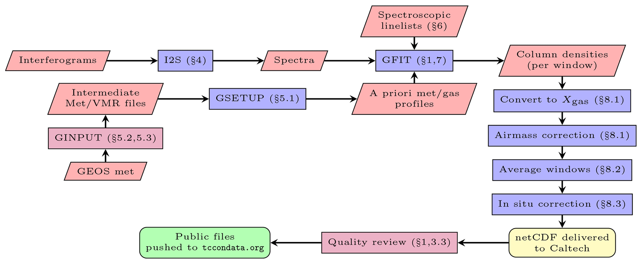
Figure 1The flow among all the components of GGG and the TCCON data. Red trapezoids (e.g “Interferograms”) represent input or intermediate data. Blue rectangles (e.g., “I2S”) represent processing steps that are part of GGG. The rounded yellow rectangle (“netCDF...”) represents a transfer step. The purple rectangles (e.g., “GINPUT”) represent centralized processing steps. The rounded green rectangle (“Public files”) indicates public-facing data. Numbers prefixed with §refer to sections of this paper.
As this paper is quite long, we provide a list of contents in Table 1 for readers to jump to sections that are of interest to them. We begin with a review of new Xgas products and changes to the data product most that are likely to be of interest to users. Next (starting with Sect. 4), for each step in the GGG processing chain, we describe the changes between GGG2014 and GGG2020. Finally, we present an uncertainty budget for GGG2020 (Sect. 9).
Notholt et al. (2022)Morino et al. (2022c)Wennberg et al. (2022c)Deutscher et al. (2023a)Iraci et al. (2022b)Wunch et al. (2022)Strong et al. (2022)Dubey et al. (2022b)Sussmann and Rettinger (2023)Liu et al. (2022)Weidmann et al. (2023)Iraci et al. (2022a)García et al. (2022)Wennberg et al. (2022e)Wennberg et al. (2022a)Shiomi et al. (2022)Hase et al. (2022)Sherlock et al. (2022a)Sherlock et al. (2022b)Pollard et al. (2022)Dubey et al. (2022a)Petri et al. (2023)Buschmann et al. (2022)Wennberg et al. (2022d)Warneke et al. (2022)Wennberg et al. (2022b)Te et al. (2022)De Maziere et al. (2022)Morino et al. (2022a)Kivi et al. (2022)Morino et al. (2022b)Deutscher et al. (2023b)Zhou et al. (2022)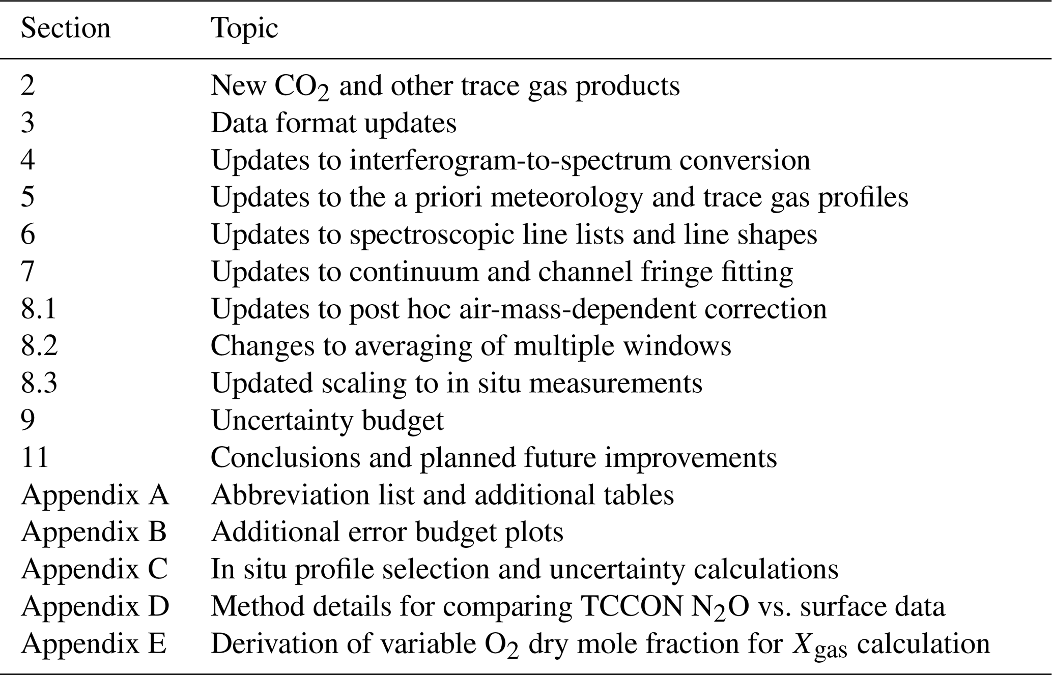
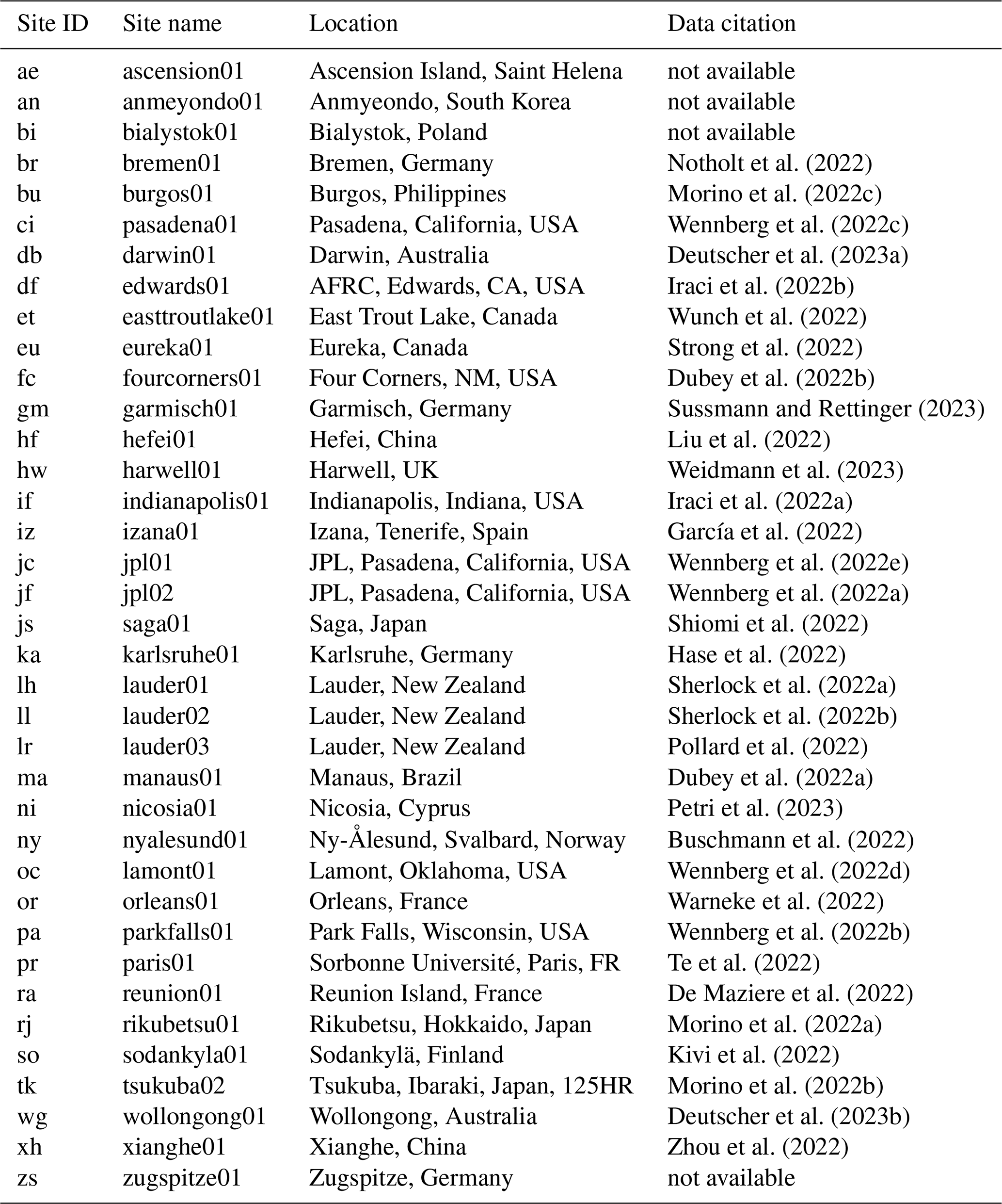
Table 2List of TCCON sites and their associated data citations as of 20 December 2022. Some sites (Lauder, JPL) have had different FTIR instruments in operation over different periods and so are listed multiple times. Sites with “not available” in the “Data citation” column did not have GGG2020 data available at time of final publication.
GGG2020 introduced dry mole fractions retrieved in two new windows: the band between 4809.74 and 4896.0 cm−1, with higher-intensity absorption than the 6330 band, and a band with weaker absorption between 6041.8 and 6105.2 cm−1. We refer to these as lCO2 (for “lower” CO2) and wCO2 (for “weak” CO2), respectively. Figure 2 shows how these two windows (plus the windows for the standard TCCON product) align with the strong and weak CO2 windows used by OCO-2 and OCO-3. These are reported as separate CO2 products ( and ) and are not averaged together with the standard TCCON product. Figure 3 shows the column averaging kernels (AKs) and CO2 absorption lines in these two windows. The lCO2 AKs increase toward the surface, while, at small slant Xgas amounts (i.e., small solar zenith angle), the wCO2 AKs are greater in the stratosphere than in the lower troposphere. This is because, as seen in Fig. 3b and d, the CO2 absorption lines in the lCO2 band are mostly saturated at the line center, while the wCO2 lines are not. When used together with the standard TCCON product (which has an AK profile that is more constant with altitude than the wCO2 or lCO2 products; see Fig. 5), this provides the potential to separate changes in CO2 at the surface from those in the free troposphere or stratosphere (Parker et al., 2023).
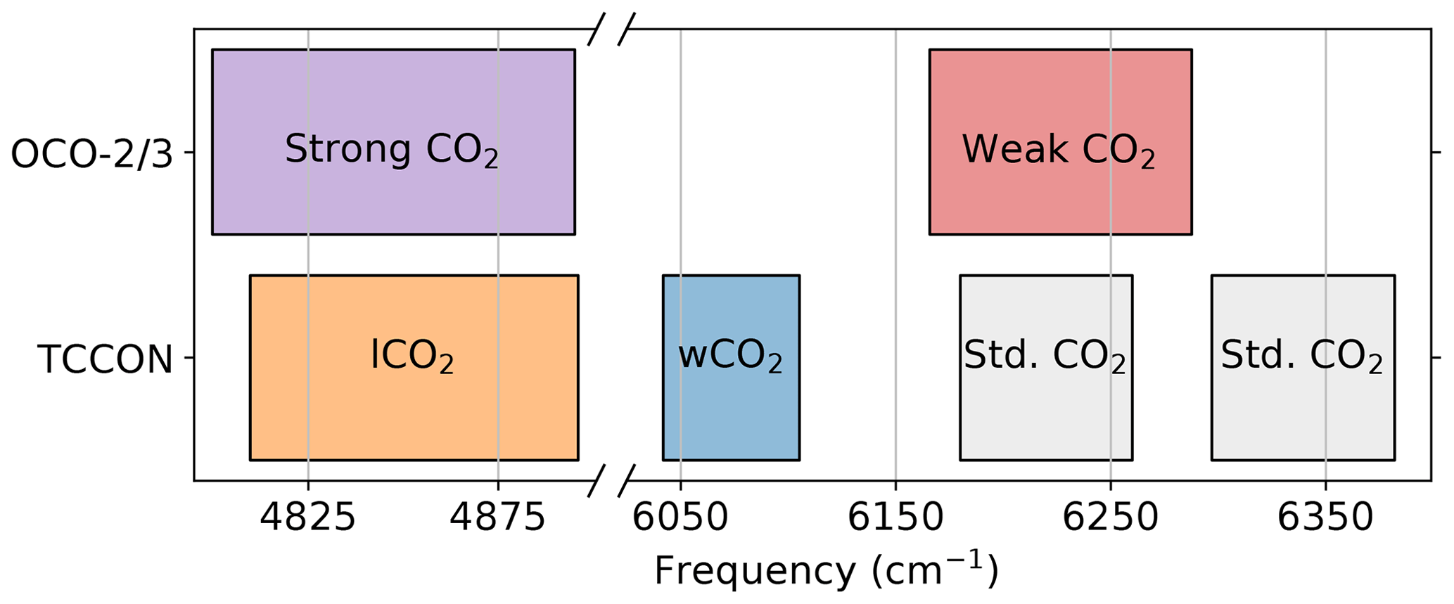
Figure 2Frequency ranges of the TCCON CO2 windows (those for the standard product, as well as for the two new products discussed in Sect. 2) compared to the frequency ranges of the OCO-2 and OCO-3 CO2 windows (Crisp et al., 2021).
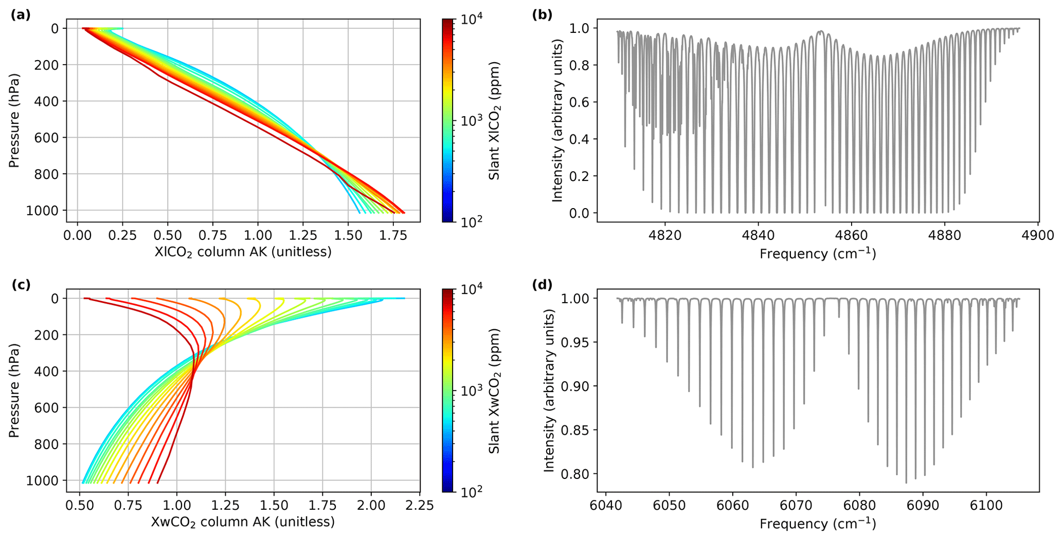
Figure 3Column averaging kernels (a, c) and calculated CO2 absorption lines (b, d) in the lCO2 (a, b) and wCO2 (c, d) windows, respectively. The absorption lines in panels (b) and (d) are for a TCCON spectrum measured at solar zenith angle = 39.684° in July 2004 at Park Falls, WI, USA. In panels (a) and (c), the different colors indicate AKs for different slant Xgas amounts. “Slant Xgas” is a measure of total absorber column along the light path. See Sect. 3.1 for details.
For wCO2, we chose not to use the second weak band around 6500 cm−1 for reasons detailed in Sect. 8.1. For lCO2, we did not use the strong band around 4900 cm−1 because the lines are so strong that the retrieval would be more sensitive to errors in the line shape and zero-level offsets in the interferograms.
Beginning with GGG2020, experimental mid-IR data products will be available from select TCCON sites equipped with an InSb (indium antimonide) detector that enables measurements in the 1800 to 4000 cm−1 frequency range. Gases observed in this range include, but are not limited to, O3, N2O, CO, CH4, NO, NO2, carbonyl sulfide, formaldehyde, and ethane. These products offer the potential to extend the applications of TCCON data to new areas of research. However, currently, these data do not have any post-processing corrections for air mass dependence (Sect. 8.1) or scaling to in situ data (Sect. 8.3) applied.
3.1 AK binning
The publicly available GGG2020 TCCON files now include one averaging kernel (AK) per observation. For a description of how these column AKs are calculated by GGG, see Sect. 3.5 of Roche (2021). This is a change from GGG2014, where the public files included a table of canonical AKs for a limited set of SZAs and where users were required to interpolate the AKs to the SZA of each spectrum. This was done in response to user requests to simplify the use of the averaging kernels. This does not mean that averaging kernels are computed by GGG for every TCCON observation (they are not). Internally, we still use a table of precomputed AKs, which are interpolated as needed to provide per-spectrum AKs in the public files. This affords significant savings in data storage as the files GGG requires to compute the AKs are very large.
Though users of public TCCON data no longer need to know how the AK tables are structured, there are two changes from GGG2014 that we wish to document here.
First, in GGG2020, the bin coordinate has changed from solar zenith angle (SZA) to slant Xgas, which is defined as follows:
where “airmass” is the unitless ratio of slant to vertical column calculated by GGG in the O2 window and Xgas is the column-average dry mole fraction of the gas of interest. Using slant Xgas as the bin coordinate correctly accounts for cases where the dynamic range of a gas's concentrations is large enough to change the AK at a single SZA. This can be seen in Fig. 4. For CO2 (Fig. 4a, b), the AKs vary smoothly and monotonically with either SZA or slant . However, for H2O, because the mixing ratios vary by orders of magnitude, the AKs do not vary simply with SZA (Fig. 4c) but do with slant (Fig. 4d). Therefore, slant Xgas was adopted as the binning coordinate for all AKs for consistency.
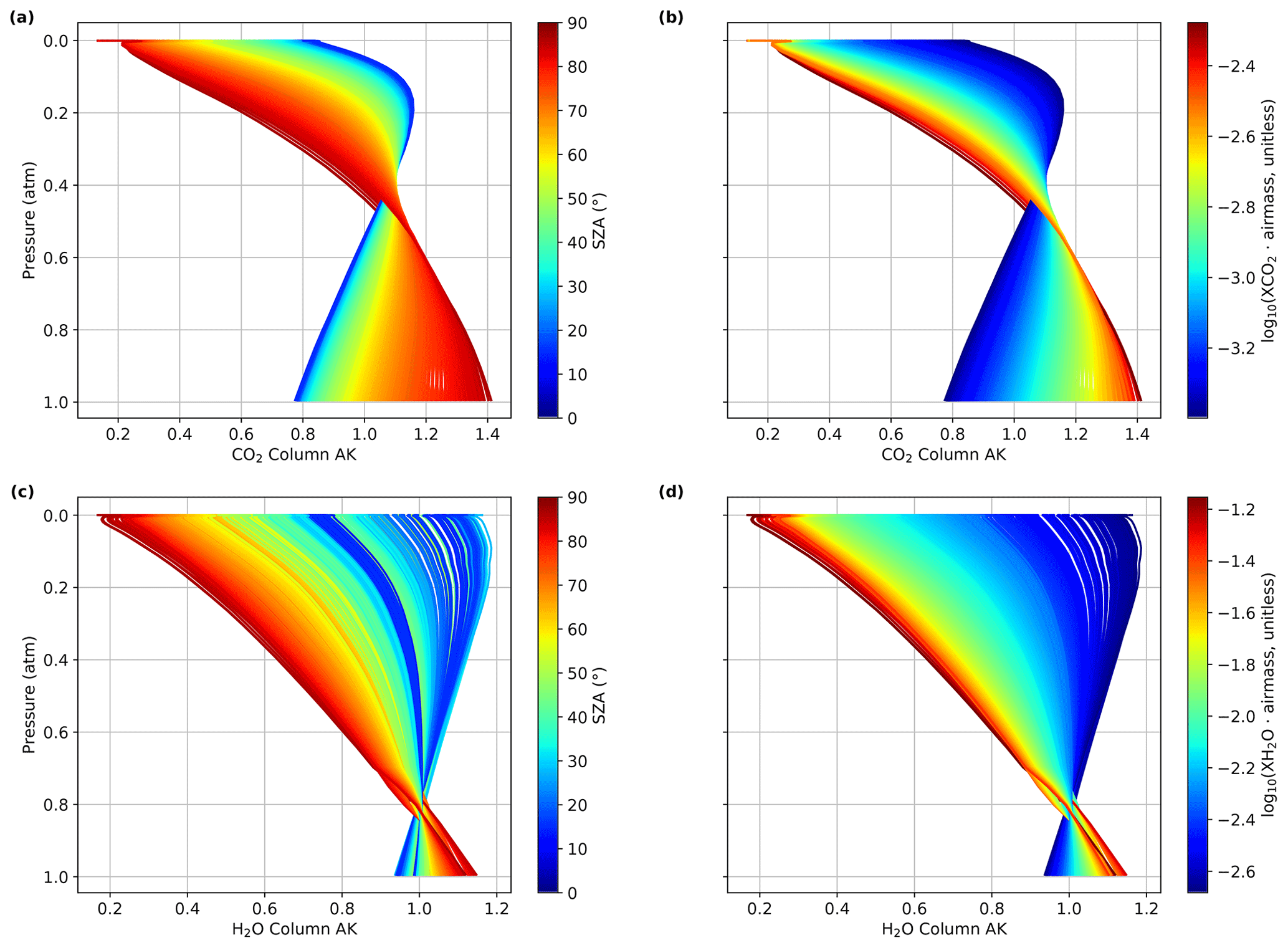
Figure 4CO2 and H2O AKs from 4 d (days) of measurements at the TCCON site in Lamont, OK, USA. (a) CO2 AKs binned by SZA. (b) CO2 AKs binned by slant . (c) H2O AKs binned by SZA. (d) H2O AKs binned by slant .

Figure 5Precomputed column AKs for TCCON Xgas products: (a) , (b) , (c) , (d) , (e) XHF, (f) , (g) , (h) XCO, (i) , and (j) XHDO.
Second, in order to provide per-spectrum AKs in the public TCCON data files without significantly increasing the file size, it was necessary to ensure that observations with similar slant Xgas values had identical AKs so that the netCDF compression algorithm could operate effectively. We achieved this by “quantizing” the slant Xgas values that we interpolated the AKs to; that is, we select 500 slant Xgas values that cover the expected range of slant Xgas plus 50 additional points to cover extreme values. Each observation then uses the AK corresponding to the one of those 550 slant Xgas values that is closest to its true slant Xgas value. This scheme keeps the difference between the quantized and full-resolution AKs to <1 % in 90 % of observations while only increasing the file size by ∼20 %.
3.2 A priori profiles and AK corrections
As described in Sect. 5.3, the a priori profiles reported in the published GGG2020 netCDF files are in units of wet mole fraction. When applying an averaging-kernel correction to calculate the Xgas value that would be retrieved by TCCON for an arbitrary gas profile, that gas profile must be converted into units of wet mole fraction. This can be done using either the TCCON H2O a priori profile provided or an H2O profile measured or modeled coincidentally with the gas profile for which an Xgas value is desired. Users who are unsure which is appropriate for their application are encouraged to reach out to the TCCON network chairs (listed at https://tccon-wiki.caltech.edu/Main/SteeringCommitteeMembership, last access: 22 April 2024) for assistance.
3.3 Changes to quality flags
As in GGG2014, a retrieval is flagged as being poor quality if any of the retrieved Xgas or Xgas error values or the ancillary variables pertaining to instrument operation or local observation conditions are outside of expected ranges. Such spectra are not included in the publicly available data files. In GGG2020, spectra may also be flagged as poor quality and withheld if one of the following criteria is met:
-
The staff at the TCCON site identify a hardware issue affecting that spectrum.
-
During pre-release data review, a time period containing that spectrum is identified as being out of family for TCCON data.
The latter case focuses on a smoothed time series of Xluft and DIP. DIP is a measure of nonlinearity in the detector or signal chain (Sect. 4.1). Xluft is a diagnostic for retrieval biases (see Sect. 6.3 for a detailed definition). As shown in Sect. 8.3 and Sect. 9, deviation of Xluft from the network median correlates with bias in the other Xgas products. Therefore, when a 500-spectrum rolling median of Xluft falls consistently outside the nominal range of 0.995 to 1.003, that time period is rejected as the Xgas products will likely have biases larger than the required TCCON accuracy. Likewise, testing has shown that increasing the magnitude of DIP increases bias in (Fig. 6). In most cases, data where DIP consistently exceeds during the initial quality assessment will be reprocessed with a nonlinearity correction (Sect. 4.1) applied to remove this bias. In very rare cases, if such reprocessing is not possible, the data are removed in order to keep the bias at less than 0.25 ppm.

Figure 6Detector nonlinearity can cause a bias in . This figure shows an example of the difference between the retrieved after correcting the nonlinearity and prior to the nonlinearity correction as a function of the DIP parameter, which is a proxy for nonlinearity. Prior to correction, the Indianapolis data had DIP values that were almost exclusively negative. To limit the bias caused by nonlinearity to less than 0.25 ppm, the absolute value of the DIP must be smaller than 0.5.
There have been substantial code changes and streamlining of common code in i2s, the interferogram-to-spectrum conversion subroutine. The main substantive improvements to the code are in the handling of detector nonlinearity, the phase correction, and other changes.
4.1 Detector nonlinearity
The largest signals in an interferogram generated by a Fourier transform spectrometer are found near zero path difference (ZPD), where light from all wavelengths constructively interferes. The modulated signal levels drop significantly away from the ZPD. If the detector measuring the interferogram has a nonlinear response, the variations in the signal near the ZPD will be more distorted than in the rest of the interferogram. This causes a discrepancy between the low-resolution spectral envelope (diagnosed near the ZPD) and the high-resolution spectral lines (diagnosed at larger path differences). Nonlinear detector responses can be strongly pronounced or subtle, and several improvements to i2s have been made to address these situations.
We have implemented a check early in i2s processing to remove interferograms affected by signal chain saturation, an extreme form of nonlinearity. If the signal intensity is too large, the ZPD signal will reach the maximum value permitted by the detector electronics. We call this interferogram saturation, and this causes irreversible loss of information. Such saturation is rarely found in the TCCON spectra and is straightforward to resolve once it has been identified. To mitigate signal chain saturation, we carefully set the pre-amplifier gain such that, even under the most intense illumination, the signal chain does not saturate. To avoid detector saturation, we limit the number of photons incident on the detector through reducing the field stop or aperture stop diameter or by placing an optical filter in the beam. Because this effect depends on sunlight intensity, saturation is more likely to occur near noon than later or earlier in the day. It is also seasonally dependent or is dependent on the amount of water vapor in the atmosphere. In GGG2020, we have implemented a saturation check to discard any saturated interferograms based on the maximum and minimum values of their signal.
There are more subtle detector nonlinearity effects that do not necessarily result in interferogram saturation but can adversely affect the retrievals. We now compute and store a detector nonlinearity diagnostic variable (DIP) as part of the regular TCCON data processing. Keppel-Aleks et al. (2007) described the solar-intensity variation correction applied to the TCCON interferograms that has been part of the TCCON processing software since 2007. In this correction, a low-pass-filtered interferogram is used to re-weight the original AC interferogram, largely removing the impacts of solar-intensity fluctuations during a measurement. As part of this work, Keppel-Aleks et al. realized that detector nonlinearity becomes observable in the low-pass-filtered interferogram as a symmetrical reduction in intensity, which we term DIP, near the ZPD (see Fig. 6b in Keppel-Aleks et al., 2007). The magnitude of this DIP is a diagnostic of the severity of detector nonlinearity and is now computed, stored, and reported as part of the routine TCCON processing.
Detector nonlinearity in the Sodankylä TCCON data persisted from early in their record until the problem was found in 2017. The problem in the early data was resolved by applying the nonlinearity correction developed by Hase (2000) directly to the interferogram before transforming it into a spectrum. This correction process and its results are described in detail in Appendices A and B of Sha et al. (2020). In that paper, the authors show that the nonlinearity caused a bias in of about 0.5 ppm in the 2017 Sodankylä data. After 2017, the problem was resolved by optically limiting the light entering the interferometer.
We now use the DIP diagnostic during the quality control step to identify all TCCON spectra affected similarly by nonlinearity. Once such data are identified, the correction process described in the previous paragraph is applied to the afflicted data. We are in the process of incorporating the correction process as a standardized part of the interferogram-to-spectrum processing to make this process easier to complete in the future.
At a few sites, DIP is consistently observed to be positive – that is, the detector appears to have a supralinear response rather than the traditional saturation response seen at, for example, Sodankylä. The procedure described in the last paragraph is not effective in correcting the supralinear behavior as it has a different physical cause than the sublinear behavior. Based on tests performed at the Garmisch TCCON site, our current hypothesis is that this behavior results from overfilling the detector element with the light beam (Corredera et al., 2003), and the magnitude of the effect varies from detector to detector. Another possible cause of supralinearity in detectors can come from absorptive layers on the InGaAs active region itself (Fox, 1993), but we do not yet have evidence that this is occurring in our instruments.
4.2 Phase correction
Sampled interferograms are always asymmetrical, either because the sampling grid does not include the ZPD position or because the underlying continuous interferogram is already asymmetrical even before it is sampled. This asymmetry causes the resulting, post-FFT, complex spectrum to have substantial imaginary terms. A phase correction is necessary to resample the interferogram such that it is sampled symmetrically about the ZPD, resulting in a computed spectrum that has the signals of interest in the real component, and only the noise is divided between both the real and imaginary components.
If we used a power spectrum (), avoiding phase correction, it would compute a spectrum that is entirely real but would retain all of the noise in the real and imaginary components of the spectrum. Therefore, the final noise level in a power spectrum would be a factor of greater than in a phase-corrected and Fourier-transformed spectrum. Additionally, in a power spectrum, saturated (zero-intensity) regions would no longer be centered at zero as any noise present is rectified and so made all positive. For these reasons, we compute a phase correction.
We use the phase correction method described by Forman et al. (1966), with a spectral domain convolution as described by Mertz (1965, 1967). The phase correction is performed using a low-resolution double-sided interferogram, apodized with a cos 2 function, to compute the angle between the real and imaginary components of the spectrum. This angle is a smoothly varying function of wavenumber and is called the phase curve. Its counterpart in interferogram space is called the phase correction operator. In regions of the spectrum with sufficient signal, the phase curve is well defined, but where the spectrum is blacked out by water vapor, another strong absorber, or an optical component, it can become undefined. Therefore, to compute the phase correction operator, we need to set a signal threshold so that we can compute a well-behaved phase curve across the spectral region of interest. We interpolate the phase curve linearly across the blacked-out regions of the spectrum where the phase curve is below the signal threshold. The phase curve is interpolated to 0 at both 0 cm−1 and the Nyquist frequency (15 798 cm−1).
In GGG2014, several TCCON stations showed retrievals of Xgas with systematic differences between spectra generated from interferograms collected while the scanning mirror moves away from zero path difference (forward scans) and while the scanning mirror moves toward zero path difference (reverse scans). These differences are typically less than 0.5 ppm in , but with larger differences observed at the Ny Ålesund, Eureka, Paris, and Zugspitze TCCON stations. This forward–reverse bias was tracked down to the phase correction operator and, more specifically, the minimum signal level threshold for which the phase operator is calculated.
To address this issue, we lowered the phase curve threshold from 0.02 (2 %, in GGG2014) to 0.001 (0.1 %, in GGG2020) of the peak spectral signal, which improves the consistency between forward and reverse scans. This eliminates the observed bias in between forward and reverse scans but is not a fully general solution to the underlying problem. In a future version of i2s, we hope to develop a phase correction scheme that is independent of the signal level.
4.3 Improved EM27/SUN support
We now make better use of the entire interferogram collected by the spectrometer in i2s. In typical linear single-passed Fourier transform spectrometers (such as those used by TCCON), we collect most of our interferometric data between the zero path difference (ZPD) and the maximum optical path difference (MOPD) positions of the scanning mirror. However, in order to perform a phase correction, a small amount of data must be collected on the other side of the ZPD, which we call the “short arm” of the interferometer. The “long arm” is the section from the ZPD to the MOPD.
I2S now has the capability to process interferograms as single sided (using data only from one side of the ZPD, usually the long arm) or double sided (using data from both sides of the ZPD, namely the long and short arms). When processing an interferogram as double sided, the optical path difference (OPD) on either side of the ZPD must be the same. This means that, for standard TCCON processing, I2S will always choose to process the interferogram as single sided because the long arm is much longer (≥ 45 cm) than the short arm (typically 0.2 to 5.0 cm). However, for spectrometers such as the EM27/SUNs, where the OPD is more symmetrical about the ZPD, I2S can process the interferogram as double sided, which avoids discarding useful data from the other side of the ZPD.
5.1 Modified retrieval grid
In GGG, the retrieval is done on a fixed-altitude grid. In GGG2014, the altitude grid had a constant spacing of 1 km, with 71 levels between 0–70 km above sea level. In GGG2020, the grid was updated to 51 levels between 0–70 km above sea level, with spacing increasing away from the surface following the expression below:
where zi is the altitude of the ith level in kilometers. As the altitude grids are fixed to sea level, this does mean that some sites have some levels below the terrain; these are not included in the integration.
5.2 Meteorological updates
In GGG2014, the a priori H2O, pressure, density, and temperature profiles were derived from NCEP 6-hourly reanalyses. In GGG2020, these profiles are now derived from the GEOS 5 FP-IT 3-hourly product in addition to potential temperature, potential vorticity, O3, and CO profiles. GGG2020 uses the nearest profile in time, changing every 3 h, to better capture changes throughout the day. The potential vorticity profiles are used to derive equivalent latitude profiles based on the equation in Allen and Nakamura (2003). Equivalent latitude is used in deriving the stratospheric part of the a priori trace gas concentration profiles (Laughner et al., 2023). GGG2020 will transition to the GEOS IT product when it replaces GEOS FP-IT; an analysis to quantify the impact of that change on TCCON Xgas products is planned.
5.3 Trace gas profile updates
GGG2020 includes a substantial redesign of the algorithm that generates the CO2, CH4, N2O, HF, CO, and O3 a priori profiles. Generating these profiles is now handled by GINPUT, a separate program from GSETUP. The GINPUT algorithm is described in detail in Laughner et al. (2023). Briefly, the CO2, CH4, and N2O profiles are tied to the long-term records from the NOAA observatories in Mauna Loa, Hawaii, and American Samoa (Lan et al., 2022b, a, c) in order to ensure that the growth rates of these gases are correctly accounted for. Individual profiles are produced based on the mean transport time between the profile location and the Mauna Loa and American Samoa observatories and (in the stratosphere) chemical loss. HF profiles are derived from CH4 profiles using the HF–CH4 relationships previously identified by Washenfelder et al. (2003) and Saad et al. (2014, 2016). CO and O3 profiles are drawn from the GEOS FP-IT chemical product2 (Lucchesi, 2015), with adjustments in the stratosphere to better match observations. See Laughner et al. (2023) for details on these adjustments.
One additional change compared to GGG2014 is that the a priori profiles are now given in units of wet, rather than dry, mole fraction. This is necessary as GGG calculates absorber number densities as the prior wet mole fractions times the number density of air, which is assumed to include water. The a priori profiles provided in the published data files are also in units of wet mole fraction. Thus, whenever one compares GGG2020 a priori profiles in the published netCDF files with other sources, care must be taken to ensure that the comparisons convert both profiles to the same (wet or dry) mole fractions. Note that the column-average Xgas values are always reported in units of dry mole fraction.
6.1 Telluric and solar line lists
As described in Toon et al. (2016), the telluric line list (atm.161, Toon, 2022c) is a “greatest hits” compilation based heavily on HITRAN predecessor lists but not necessarily on the latest HITRAN version for all bands and gases. As new line lists become available, they are evaluated using laboratory and atmospheric spectra and are compared with earlier HITRAN line lists and the current atm.161 line list, which is updated if the new line list represents an improvement in any spectral regions, as determined by (1) improved fitting residuals, (2) better consistency of retrieved gas amounts from different windows and bands, and (3) reduced air mass dependence of the retrieved gas amounts. Additionally, ad hoc empirical corrections are performed for some lines, bands, and gases to fix obvious errors. Since the GGG2014 version of the line list, there have been many improvements to the H2O and HDO spectroscopy throughout the main TCCON region (4000 to 8000 cm−1). Water vapor is an important interferer in almost all windows, as is CH4, which has also undergone substantial ad hoc correction, but not in the 2v3 band (5800 to 6200 cm−1), where CH4 itself is retrieved.
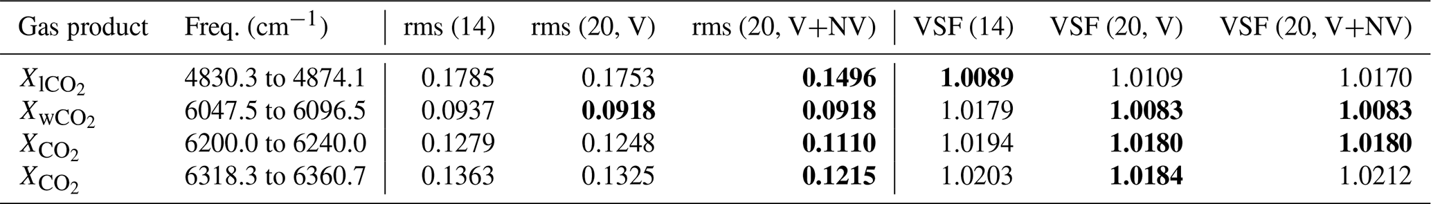
Table 3 shows how the spectral residuals (i.e., the difference between the observed and simulated spectra for the retrieved state) and VMR scale factors (VSFs, the ratio of the retrieved to the a priori gas column) have progressed between the GGG2014 and GGG2020 line lists. These results are for spectra of gas cells with a known amount of CO2 and so are restricted to CO2. For all the CO2 bands used by GGG2020, the spectral residuals show clear reductions in the GGG2020 line list, combining Voigt and non-Voigt lines (see Sect. 6.2 for details of the non-Voigt line shapes), compared to GGG2014. The mean bias in line strengths, as indicated by the VSF values, was more varied: two windows had less bias (with VSFs closer to 1), but the other two had slightly larger bias. However, such biases are removed by scaling to match in situ data (Sect. 8.3); thus, while removing such biases with improved spectroscopy is desirable, their presence has little impact on the TCCON data.
Table 3Results of test retrievals on known amounts of CO2 in a cell with three different line lists. “(14)” indicates the GGG2014 line list, “(20, V)” indicates the GGG2020 line lists without the non-Voigt lines discussed in Sect. 6.2, and “(20, V+NV)” indicates the full GGG2020 line list (with non-Voigt lines included). The window does not have non-Voigt CO2 lines; thus, its (20, V) and (20, V+NV) results are the same. “Gas product” indicates which of the TCCON products is retrieved in each frequency window, and “Freq.” gives the span of that window. Note that these windows are used to fit laboratory cell spectra and differ slightly from those used operationally by TCCON (given in Tables A2 and A3). The “rms” columns list the root mean squared difference between observed and simulated spectra normalized by the continuum level. The “VSF” columns list the ratio of the retrieved CO2 amount to the prior amount. Since these measure known CO2 amounts in laboratory cells, VSF ≠1 indicates a systematic bias in the CO2 line strengths. For both the rms and VSF columns, the best values (closest to 0 for rms and closest to 1 for VSF) are in bold.
Improvements to the telluric line lists are communicated to the HITRAN group through spectroscopic evaluations, posted to https://mark4sun.jpl.nasa.gov/presentation.html (last access: 31 January 2024). Such evaluations are also performed on candidate line lists developed by the HITRAN group to provide feedback on the performance of those line lists before they are adopted.
The solar line list (Toon, 2022b) is completely empirical, based on high-resolution solar spectra measured by various instruments from the ground, balloons, and space. In the 4000 to 8000 cm−1 spectral region covered by TCCON, the line list is based primarily on ground-based Kitt Peak and TCCON spectra, with additional balloon-borne MKIV spectra from 40 km altitude up to 5600 cm−1. To deduce which absorption features are solar rather than telluric, we fit out the telluric spectrum as best we can. Remaining dips in the residuals are solar unless they grow with air mass, in which case they are missing tellurics.
The solar line list is not the same format as the HITRAN line list. In addition to the line position, there are parameters representing the line center absorption depth, a Doppler width, and a Lorentz width, each for disk-center and disk-integrated cases; thus, there are seven parameters in total. A simple subroutine computes a solar pseudo-transmittance spectrum from these seven parameters, providing flexibility to model disk-center, disk-integrated, or intermediate cases. Since GGG2014, the improvements in the main TCCON region have been modest, adding new weak lines (<0.1 % depth).
The solar continuum is handled separately from the line list in GGG. This is discussed in Sect. 7.
6.2 Non-Voigt line shapes for O2, CO2, and CH4
Absorption coefficient calculations were improved in GGG2020. In previous versions of GGG, absorption coefficients were calculated using a Voigt spectral line shape. Numerous spectroscopic studies (e.g., Tran et al., 2013; Hartmann et al., 2009; Gordon et al., 2017) have shown that the Voigt line shape is insufficient for use with CO2 and other molecules; thus, a more sophisticated line shape is required to improve the accuracy of the retrieval. Hence, the quadratic speed-dependent Voigt (qSDV) with line-mixing (LM) code from Tran et al. (2013) was implemented into the forward model of GGG (Toon, 2022a). Tables A2 and A3 in the Appendix list the frequency windows used in GGG2020 and contain columns identifying which windows include speed-dependent and line-mixing line shape information.
It was shown in Mendonca et al. (2016) that using the qSDV with first-order LM and adopting the spectroscopic parameters from Devi et al. (2007b) for the CO2 lines in the CO2 window centered at 6220 cm−1 and from Devi et al. (2007a) for the window centered at 6339 cm−1 resulted in an up-to-40 % improvement in both spectral-fit rms values and a reduction in the air mass dependence of the retrieved XCO2. For the CO2 band lines in the window centered at 4850 cm−1, the spectroscopic parameters from Benner et al. (2016) are used with the qSDV and first-order LM to calculate absorption coefficients. This resulted in improving the quality of XCO2 retrievals (i.e., reducing the spectral-fit rms) from this spectral region. New spectroscopic studies aimed at improving CO2 absorption coefficient calculations are ongoing. Recent studies like that of Hashemi et al. (2020) that provide spectroscopic parameters for CO2 can be tested with TCCON spectra to see if the retrievals can be improved.
TCCON CH4 is retrieved from three windows that are composed of the P, Q, and R branches of the 2ν3 CH4 band. To improve the forward model of GGG, the spectroscopic parameters from Devi et al. (2015, 2016) are used to calculate the absorption coefficients with the qSDV with full line mixing. Unlike CO2 that uses first-order line mixing, requiring that one extra parameter be added to the line list per spectral line, CH4 requires full line mixing. This requires that spectroscopic parameters from all coupled lines (i.e., a relaxation matrix) be used to calculate the effective spectral line parameters for each spectral line. In previous versions of GGG, absorption coefficients could only be calculated by reading in spectroscopic parameters line by line, making it awkward to take into account the full line mixing. GGG2020 has been updated to read in spectroscopic parameters and the relaxation matrix (supplied in Devi et al., 2015, 2016) at the same time for spectral lines that require full line mixing. More details on how this is done are provided in Mendonca et al. (2017). The improved absorption coefficient calculations for CH4 lines for the 2ν3 CH4 band have improved the quality of the spectral fits and the air mass dependence of the retrieved XCH4. The addition of full line mixing can be extended to other molecules to improve retrievals.
To improve the retrievals of O2 columns, which are required to calculate Xgas, spectroscopic parameters for the O2 singlet delta band were retrieved by fitting cavity ring-down spectra as detailed in Mendonca et al. (2019). The spectroscopic parameters derived from the cavity ring-down spectra were tested on TCCON spectra, where they were shown to slightly improve the quality of the spectral fit, as well as greatly decrease the air mass dependence of the retrieved O2 column. The study by Mendonca et al. (2019) is the first to show the need for a spectral line shape that takes into account speed dependence. Since then, newer spectroscopic studies such as those of Tran et al. (2020) and Fleurbaey et al. (2021) have shown the need to take into account Dicke narrowing and line mixing in order to fit new cavity ring-down spectra in the O2 singlet delta band. The spectroscopic parameters of Mendonca et al. (2019), Tran et al. (2020), and Fleurbaey et al. (2021) were used to fit TCCON O2 spectra in Tran et al. (2021). The study showed that the newer spectroscopic parameters slightly improved the quality of the spectral fit but that they should also be assessed on the basis of how they impact the air mass dependence of retrieved O2 columns.
This does mean that the standard 160-character-wide HITRAN line list product does not include all of the parameters required for these gases. GGG has always used a customized version of the HITRAN line list. Therefore, this need for additional parameters represents an increase in the complexity of our line list strategy but also a continuation of the same approach to use the best spectroscopic information from various sources rather than a wholly new approach.
6.3 Empirical optimization of O2 line widths
During pre-release testing, we found that a diagnostic quantity we call Xluft had a noticeable temperature dependence (Fig. 7a). Xluft is defined as follows:
where
-
is the water vapor wet mixing ratio for level k;
-
nair,k is the ideal gas number density of air at level k (calculated from temperature and pressure);
-
Δzeff,k is an effective path length for level k that accounts for the pressure-weighted contribution of that level and the surface pressure;
-
is the retrieved O2 column (with the same integration as the numerator); and
-
is the mean dry mole fraction of O2 in air, fixed at 0.2095 for GGG2020 (see Sect. 8.3.2 for a discussion on accounting for the trend in O2 dry mole fraction).
Conceptually, Xluft is a ratio of two distinct ways of calculating the column of dry air (one from surface pressure and the a priori H2O profile and one from the column of O2 retrieved in the singlet delta band – or put another way, it is the column-average dry mole fraction of dry air) and thus should not have a temperature dependence. Since dry mole fractions of O2 in the atmosphere are highly constant over space and time, this implied that either the temperature dependence or the water broadening of the O2 line widths in the forward model was incorrect as the concentration of water in the atmosphere is generally correlated with temperature.
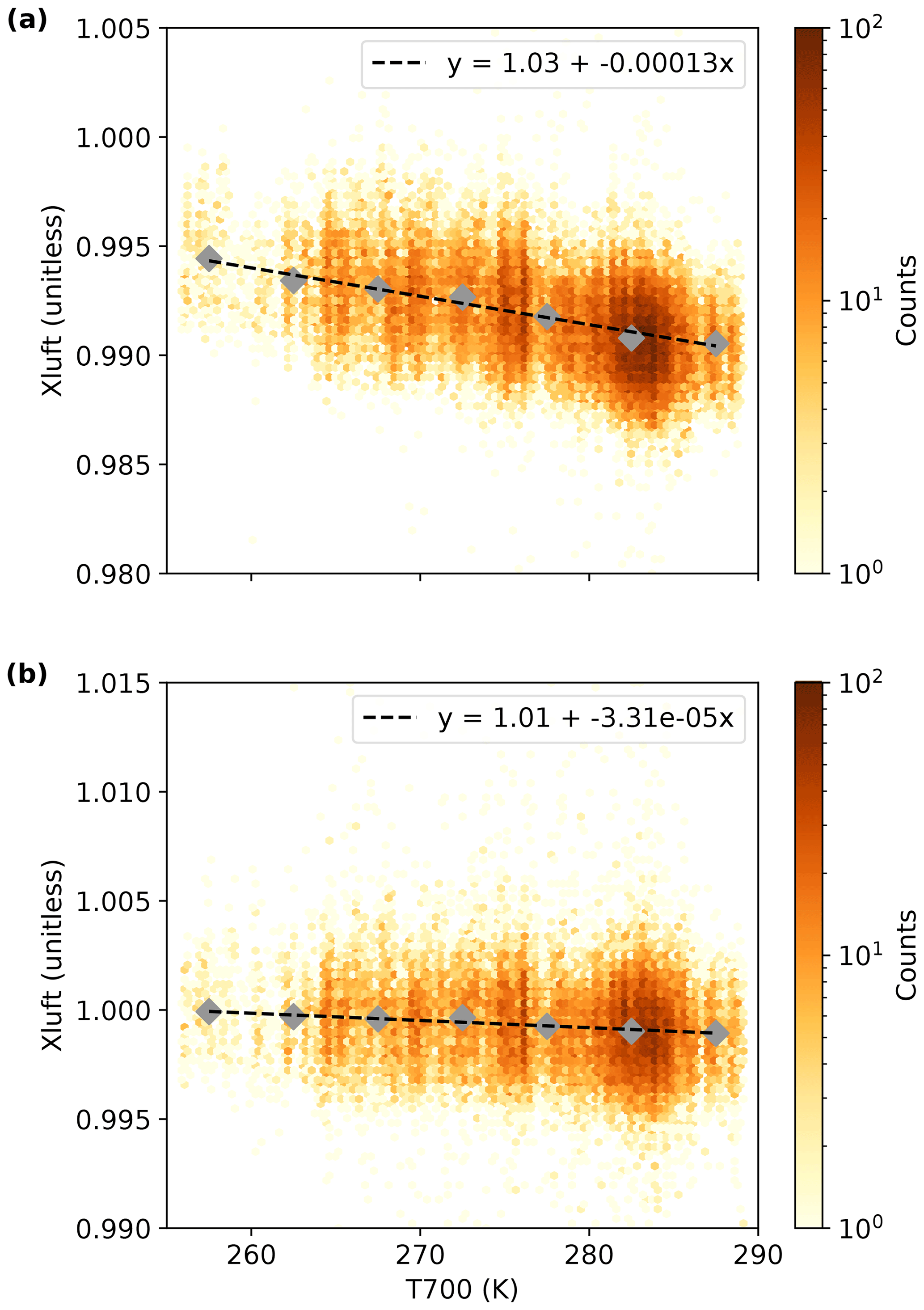
Figure 7Correlation between Xluft and temperature at 700 hPa (a) before and (b) after optimizing the O2 line broadening in terms of its water, pressure, and temperature dependencies. Note that (a) is not from the previous TCCON data version (GGG2014); it is from a preliminary beta test of GGG2020. In both panels, the colored background is a 2D histogram, the gray diamonds mark the mean Xluft in 5 K bins, and the black line is a linear fit to the gray diamonds. The data shown here are from the Lamont TCCON site, between 2 September 2017 to 30 September 2018. Note that the y-axis limits shift between the panels; this is because the mean magnitude of Xluft changed with the increase in O2 line intensities (see text) between the tests plotted in the two panels. The slope is visually comparable between the panels since the span of Xluft is the same (0.025) in both panels.
To disentangle the effect of temperature and water, we first examined data from the Darwin, Australia, TCCON station. Darwin is located in the tropics and so experiences greater water columns and a narrower range of temperatures than other TCCON sites (Fig. 8a, b). We chose approximately 14 months of data from Darwin when the instrument was performing well and processed that year three times, with water broadening set to 1.0, 1.4, and 1.8 times that of the air-broadening half-width.
To identify the optimal strength for water broadening, we examined the slope of Xluft vs. the water column in 10° SZA bins for each of these tests. Binning the data by SZA helps to separate the water dependence from air mass dependence. Figure 8c shows that a water broadening of 1.4 times that of air minimized the dependence of Xluft on water.
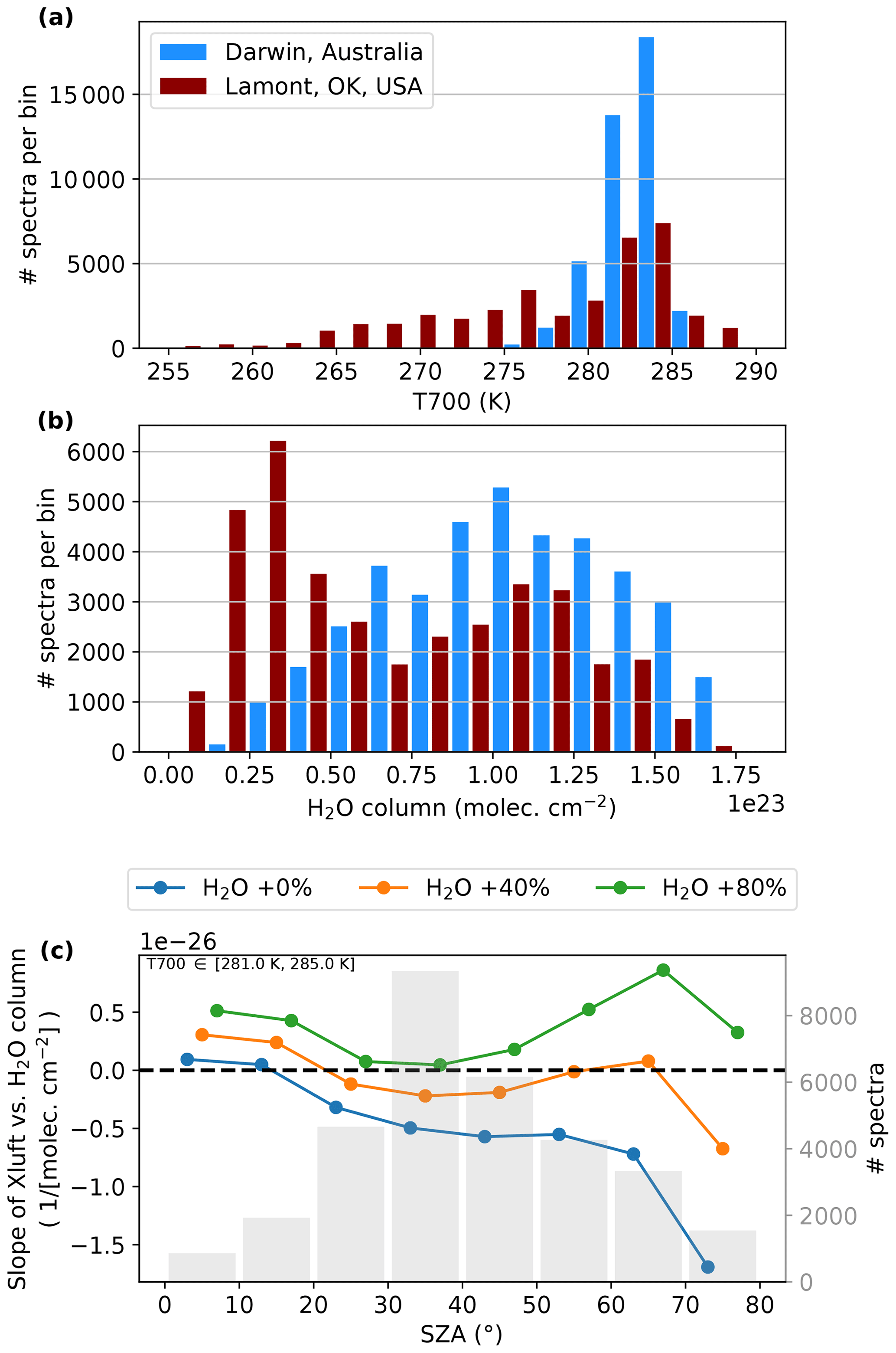
Figure 8(a) Histogram of temperatures at 700 hPa at the Darwin (located at 12.5° S) and Lamont (located at 36.6° N) TCCON sites. (b) Histogram of water column amounts at the same sites. (c) Slopes of Xluft vs. water column in 10° SZA bins at Darwin, with water broadening of O2 set to be equal to, 40 % greater, and 80 % greater than air. The gray bars give the number of spectra in each bin. The Lamont data in (a) and (b) are from the period 2 September 2017 to 30 September 2018, and the Darwin data in all bins are from 21 July 2015 to 30 September 2016.
With the water broadening optimized, we turned to the temperature dependence of the O2 line widths. Reducing the dependence of Xluft on temperature was the primary goal; however, we had to account for the interplay between the temperature and pressure dependence. In particular, our concern was that changing the temperature dependence of the O2 line widths would introduce or increase an SZA dependence by changing the average line widths.
Our solution was to simultaneously adjust both the temperature and pressure dependence of the O2 line widths. To find the optimal combination of these coefficients, we minimized a cost function of three quantities. For each quantity, we tested how the results changed using a different collection of TCCON sites:
-
the average magnitude of the slope of Xluft vs. temperature at 700 hPa (T700) across various combinations of 1–3 of the East Trout Lake, Lamont, and Park Falls sites;
-
the variance of the Xluft vs. SZA slopes across the Darwin, East Trout Lake, Lamont, and Park Falls sites;
-
the variance of the magnitude of Xluft across the same sites as in no. 2.
Our rationale was that the temperature dependence of Xluft was the most important error to eliminate; thus, minimizing its magnitude took priority. T700 is taken from the a priori meteorology data and was chosen based on the assumption that this is a reasonable metric for temperature variations in the free troposphere (∼ 800 to 200 hPa), containing the majority (∼ 60 %) of the O2 column. We then minimized the variance in slopes of Xluft vs. SZA across different TCCON sites because GGG already has a well-tested program to remove spurious SZA dependencies in the output Xgas products so long as those dependencies are the same across sites. While minimizing the magnitude of the SZA dependence itself would have been preferable, we were not certain there would be enough flexibility in the Xluft–O2 spectroscopy relationship to simultaneously minimize the temperature and SZA dependencies. Similarly, we minimized the variance in Xluft itself because the average magnitude of Xluft depends on the strengths of the O2 lines rather than the pressure and temperature effects on line width that were adjusted in this initial experiment. Therefore, while we ideally want Xluft=1, this first step did not involve optimizing the spectroscopic parameters that can achieve that. We do adjust the O2 line strengths separately, as noted at the end of this section.
To carry out this optimization, we ran approximately 1 year of data from four TCCON sites (Darwin, Australia; East Trout Lake, Canada; Lamont, OK, USA; Park Falls, WI, USA) multiple times. In each test, we scaled the temperature dependence, pressure dependence, or both of all lines in the O2 band, covering a reasonable range of estimates from the literature. We could then interpolate between these test runs to estimate the three cost function quantities for any pressure- or temperature-broadening coefficients, and from that, we could find the combination of coefficients that minimized the overall cost function. Note that we did not use Darwin data to calculate the Xluft versus T700 slopes for the cost function as the small range of temperatures that Darwin experiences (Fig. 8a) makes it difficult to get reliable fits versus temperature.
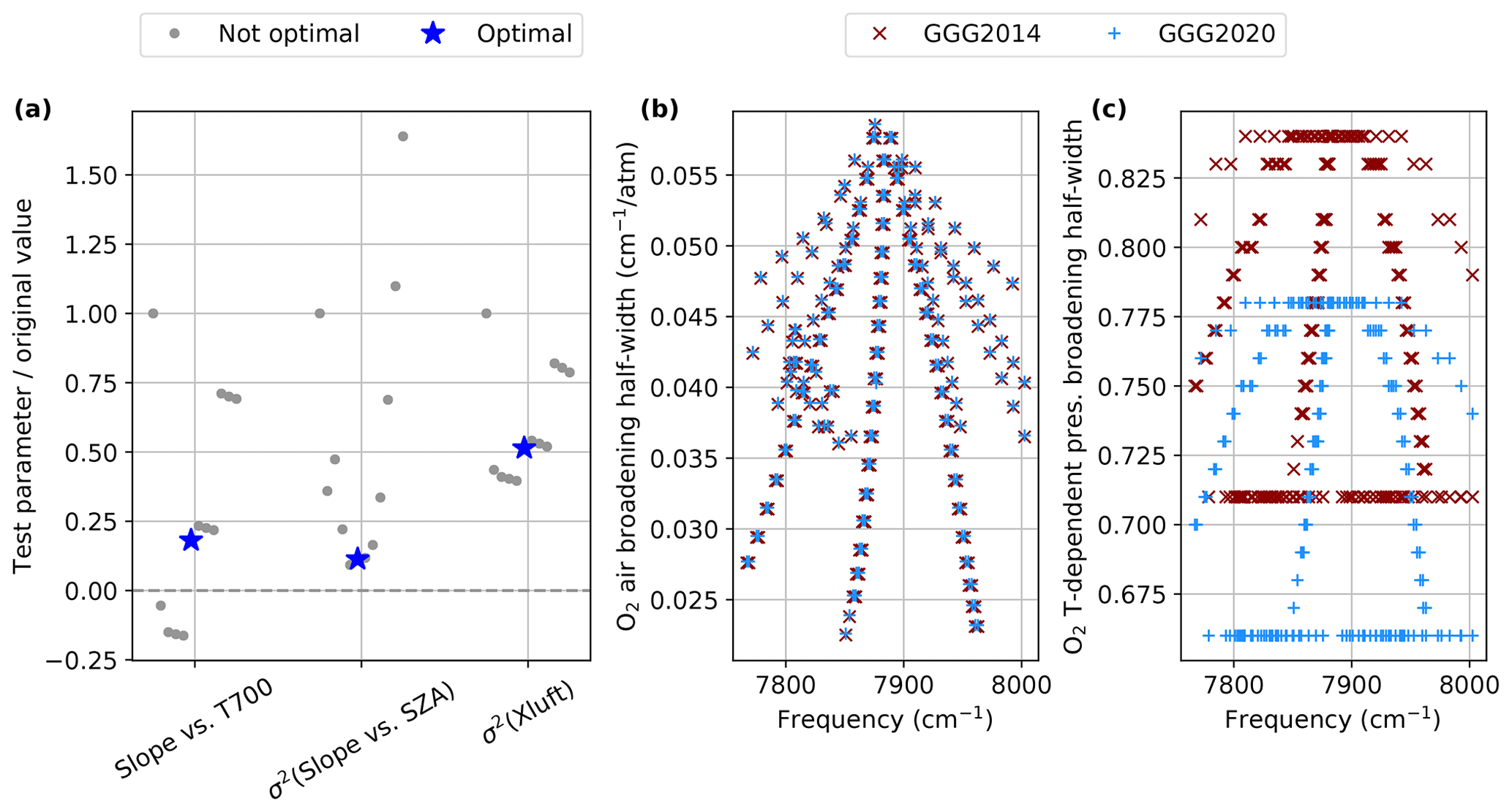
Figure 9Result of the O2 spectroscopy optimization. (a) The values of each criterion for each test using different values of pressure- and temperature-broadening coefficients. The values are normalized to their values in the baseline test (before optimizing the O2 spectroscopy). The points within each parameter are spread horizontally for clarity. (b) The air-broadening half widths used in GGG2020 (after optimization) compared with GGG2014. The mean GGG2020 GGG2014 ratio is 1.0025; thus, the points are barely different on this scale. (c) As in (b) but for the temperature-broadening coefficient. The mean GGG2020 GGG2014 ratio is 0.9323.
The results of the optimization are shown in Fig. 9. Figure 9a shows how the three criterion described above (slope of Xluft vs. T700, variance in slope of Xluft vs. SZA, variance in Xluft) varied across the tests performed with different pressure- and temperature-broadening coefficients. The values are normalized to their respective pre-optimization values. We found that the best combination of coefficients reduced the slope of Xluft vs. T700 by 82 %, the variance in Xluft vs. SZA slopes across TCCON sites by 89 %, and the variance in Xluft itself by 49 %. The optimized air-broadening half-widths and temperature dependence coefficients for GGG2020 are shown in panels (b) and (c) of Fig. 9, respectively, with GGG2014 values for comparison. The air-broadening half-widths were increased by 0.25 %, and the temperature dependence coefficients were decreased by 6.77 %. The effect on the Xluft vs. T700 relationship is shown in Fig. 7b, where, although not reduced to zero, the slope is reduced by a factor of 4 compared to its pre-optimization value.
Finally, the O2 line intensities were increased by ∼1 % to bring Xluft closer to 1. This effect is apparent in Fig. 7, where the pre-optimization values are between 0.990 and 0.995, but the post-optimization Xluft in panel (b) is near 1. Across the TCCON network, we determined that the median Xluft is 0.999; therefore, we use that as the benchmark for ideal Xluft.
TCCON spectra are a combination of narrow features due to solar and telluric absorptions superimposed on the much broader spectral responses of the instrument3 and the solar Planck function (the continuum). To accurately fit the telluric features of interest, all other components of the spectrum must be accurately modeled simultaneously. Since TCCON spectra are not radiometrically calibrated, the continuum can vary from instrument to instrument or even from day to day (if optical components are inserted or replaced); therefore, a general approach was needed to model the continuum. Prior to GGG2014, the continuum was fitted with only two terms (mean and slope) over the < 100 cm−1 wide windows used to retrieve atmospheric gases. To make use of wider spectral windows, it became necessary to include additional higher-order terms in the model of the continuum to account for optical components within the instrument (e.g., detectors, optical filters, beam splitters) that induce curvature in the spectral response (e.g., Kiel et al., 2016b). In GGG2014, we implemented the ability to fit higher-order polynomials to the continuum level using discrete Legendre polynomials, although this capability was not uniformly used in the GGG2014 TCCON data processing (Wunch et al., 2015). We use Legendre polynomials because they are orthogonal, whereas standard polynomials are not. Higher-order Legendre polynomials are now used widely in the GGG2020 spectral windows to better account for continuum shape changes between instruments and over time. The continuum curvature fitting option is not intended to fit out spectroscopic deficiencies; they will be air mass dependent and so should be fixed separately. The default polynomial order in GGG2020 for each window has been chosen to capture the continuum shapes of all sites in GGG2020 and to reduce the spectral residuals without over-fitting the spectrum. The default order for each window is listed in Tables A2 and A3.
7.1 Channel fringe fitting
Parallel optical surfaces delay a small fraction of the transmitted beam, which subsequently interferes with the main, un-delayed beam, resulting in a small periodic modulation of the spectral signal. This modulation has an amplitude of R2, where R is the reflectivity of each surface, and a period of cm−1, where n is the refractive index of the optic, d is its thickness (in cm), and θ is the angle to the normal.
For decades, GFIT has had the capability to fit a channel fringe to determine its amplitude (as a fraction of the continuum), its period, and its phase and then remove it from the measured spectrum during the spectral fitting. This capability was not used by TCCON until GGG2020, when spectral fits from some sites were noticed to exhibit the tell-tale periodicities in the residuals. Left untreated, channel fringes can seriously bias the retrieved gas amounts by an amount that can vary from instrument to instrument and even over time for a single instrument, e.g., if its temperature changes.
An important code change for GGG2020 was to prevent channel fringes from being mistaken for higher-order continuum terms. This was much less of a problem for GGG2014 when we only ever fitted a straight line to represent the continuum. But now, if a particular wavelike feature in the continuum could be fitted by a higher-order polynomial or by a channel fringe, this tends to slow down convergence as the continuum fitting and channel fringe fitting vie with each other. To prevent this, a lower limit was imposed on the channel fringe period that was fittable in a given window, such that it was always narrower than the periodicities in the continuum-fitting polynomial. Hence, if we are fitting an N-term polynomial to the spectrum (called the number of continuum basis functions or NCBF) in a window of width w (in cm−1), then the period of the fitted channel fringes must be less than .
Diagnostics to detect channel fringes are reviewed as part of the quality control process before TCCON data are made public. Any channel fringes detected will be removed by adjusting the fitting before the data are released to the public archive, though this is extremely uncommon.
GGG incorporates several post-retrieval steps to (1) collate and average data (Sect. 8.2) from the individual retrieval windows into the final Xgas products and (2) correct post hoc for known errors in the forward model. There are two corrections. The first is an air-mass-dependent correction (Sect. 8.1), which aims to eliminate spurious dependence of Xgas quantities on SZA. The second is an in situ-based or air-mass-independent correction (Sect. 8.3), which aims to eliminate the mean bias in Xgas values arising from incorrect spectroscopic line strengths. These corrections are calculated from data that include all improvements discussed in the preceding sections.
In the following sections, the post-processing steps are presented in the order in which they are applied in GGG2020.
8.1 Updated air mass dependence correction
In the limit of no variation in trace gas dry air mole fraction, Xgas quantities are independent of atmospheric path length as the change in column density due to path length is multiplicative and so will cancel out between the target gas in the numerator and O2 in the denominator. However, a spurious dependence of Xgas on air mass can arise from errors in the spectroscopic forward model.
8.1.1 Changes to air mass correction approach
GGG2020, like GGG2014, applies a post hoc correction to the Xgas values to remove air mass dependences. This correction is applied to each Xgas value. It has a similar form to that in Appendix A of Wunch et al. (2011):
We use this to correct the Xgas value as follows:
In Eq. (6), ADCF (standing for air-mass-dependent correction factor) is a coefficient for each gas (in GGG2014) or each window (in GGG2020). In Eq. (5), SZA is the solar zenith angle in degrees, and g and p are coefficients chosen to best represent the SZA-dependent behavior. This form was chosen to normalize to a 90° window centered at (45+g)°. While the basic approach is the same in GGG2020 as it was in GGG2014, we made four changes to the implementation:
-
In GGG2014, column densities from different spectral windows used to retrieve a target gas were averaged first, and then a single air mass correction was applied to each gas. In GGG2020, each spectral window is air mass corrected first, and then the resulting Xgas values are averaged.
-
In GGG2014, g=13 and p=3 for all gases. In GGG2020, different values of g and p were selected for each window.
-
In GGG2014, only data from 3 TCCON sites (Park Falls, Lamont, and Darwin) were used to compute the ADCFs. For GGG2020, we use 18 sites' data.
-
In GGG2014, we did not examine the ADCF for temperature dependence. We do in GGG2020 and attempt to account for that in how we select the final ADCF values.
The rationale for the first change is clear from Fig. 10. The standard TCCON CO2 and CH4 products are derived from two and three spectral windows, respectively. Although the overall SZA dependence has a similar shape for all windows of a given gas, there are clear differences in low- and high-SZA behavior. Thus, we decided to apply an SZA-dependent correction to individual windows rather than the average Xgas value. The right panels of Fig. 10 show that applying the air mass correction significantly reduces the SZA dependence of the data.

Figure 10Variation of (a, b) the two CO2 and (c, d) three CH4 windows used by TCCON with SZA. Panels (a) and (c) are without the air mass correction applied, and panels (b) and (d) are with the correction applied. In all panels, the y axis is the column-average dry mole fraction of CO2 or CH4 derived from a single spectral window, with the central wavenumber given in the legend. The y values have the daily median values subtracted (to remove day-to-day variability), and each point represents the median of all such values in a 5° SZA bin. The gray bars give the number of observations in each 5° SZA bin (this is the same in all panels).
The rationale for the second change is that we do not know a priori the best form to represent the air mass dependence in any given window. For GGG2020, we used data from the Darwin TCCON site for all of 2015 to choose the values of g and p for each window. We used Darwin because, as a tropical site, it sees a wide range of SZAs (useful for examining SZA dependence) and water columns (useful to check for water effects on the derived air mass dependence). We used 2015 data because the instrument at Darwin was well aligned during that year.
To understand how g and p were determined, we must first explain how the ADCF in Eq. (6) is calculated for a given g and p. The ADCF is calculated by fitting the following function to each day's data:
where t and tnoon are the measurement time and solar noon time (in day of year); fc is the polynomial defined in Eq. (5); and cmean, casym, and cADCF are the fitted coefficients. This equation assumes that symmetrical variations in Xgas values around noon (fit by fc) are due to spectroscopic errors, and real variations throughout the day are antisymmetrical and will be fit by the casym term. The coefficients and their errors are calculated with a weighted least squares fit using the individual windows' Xgas uncertainties (calculated from the spectral residuals of the target gas and O2) as the weights. The ADCF for a given window is the error-weighted mean of all days' cADCF values.
8.1.2 Determination of ADCF coefficients
To find the optimal g and p values, we derived ADCFs for five subsets of the 2015 Darwin data (data with SZA > 20, 30, 40, 50, and 60°, all with H2O column molec. cm−2) for values of g between −45 and +45 and values of p between 1 and 6. We then find the combination of g and p that gives the smallest standard deviation in terms of the ADCF across all five subsets and choose that as the optimal combination. This approach assumes that the values of g and p (and thus the form of fc) which best capture the air mass dependence of a particular window will have the smallest change in ADCF as smaller subsets of data are fit.
This procedure is illustrated for the two TCCON CO2 windows in Fig. 11. In the top panels, the gray lines show the variation in ADCF with the minimum SZA in the subset of data fitted to; each line represents one combination of g and p. It is clear that the variation in ADCF is much greater for some combinations of g and p than others. The contour plots in Fig. 11 show the standard deviation of ADCF for each g and p combination. In both windows, there is a clear minimum valley. The white stars in the contour plots and thicker black lines in the upper panels show the g and p combination with the smallest standard deviation.
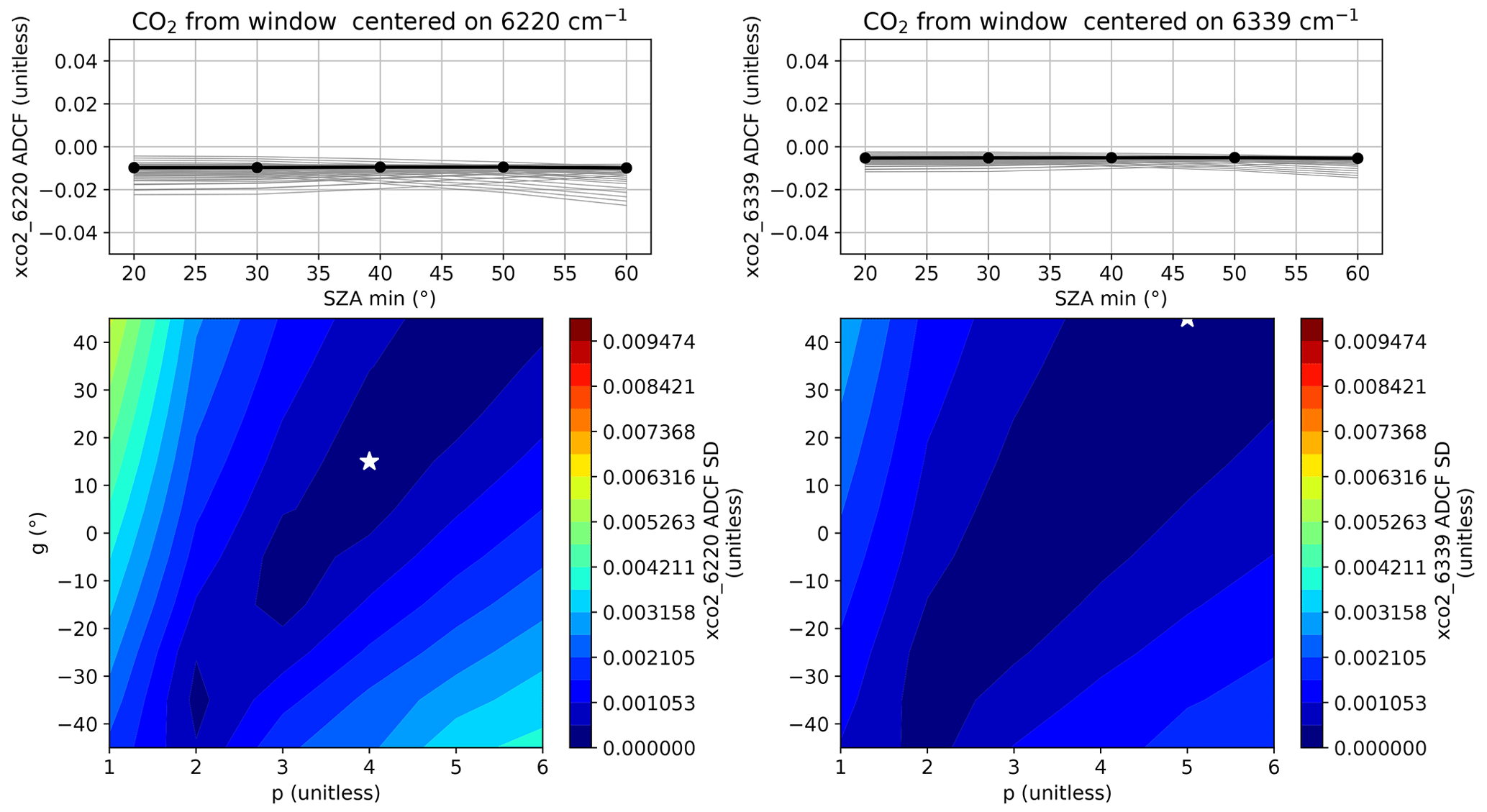
Figure 11Example of how g and p in Eq. (5) were chosen for the two TCCON CO2 windows. The left two panels are for the CO2 window centered at 6220 cm−1, and the right two panels are for the window at 6339 cm−1. The line plots at the top show how the value of the ADCF changes as we increase the lower limit in SZA for the data fitted to. Each gray line represents one combination of g and p, with the black line representing the combination with the smallest standard deviation in the ADCF. The contour plots show the standard deviation of the ADCF across different minimum SZAs for each combination of g and p. The white star represents the combination with the smallest standard deviation; it corresponds to the test show with the black line in the line plots.
The final step in selecting ADCFs for GGG2020 was to account for potentially spurious temperature dependence in the Xgas values. As we saw with O2 in Sect. 6.3, incorrect temperature dependence in the line widths introduces a temperature dependence in retrieved Xgas, which could alias into the air mass dependence. While we acknowledge that such temperature dependence of the ADCFs could be due to a real change in the atmosphere, we believe this to be unlikely for two reasons. First, the ADCF is constructed to account only for variations in Xgas that are symmetric around solar noon, and generally changes in atmospheric composition are not perfectly symmetric around solar noon. Second, as we show in Fig. 13, different windows for the same gas have different relationships between the ADCF and temperature. A real change in atmospheric composition would be more likely to show up in all windows for a given gas.
To check this, we derived ADCFs from the data of 18 TCCON sites using 2-month-long subsets of data to sample different temperatures. Figure 13 shows how the CH4 ADCFs vary with potential temperature averaged between 500 and 700 hPa (θmid) as an example. Figure 12 shows how θmid and T700 relate to assist in comparisons with Fig. 7. Here, we see that the 6002 and 6076 cm−1 windows' ADCFs have no or little temperature dependence (Fig. 13b, c), but the 5938 cm−1 window has a clear temperature dependence. For each window, we use the value of the fit to this data at θmid=310 K as the final ADCF value; 310 K was chosen as it is approximately the midpoint temperature for the TCCON network, as can be seen in Fig. 13.
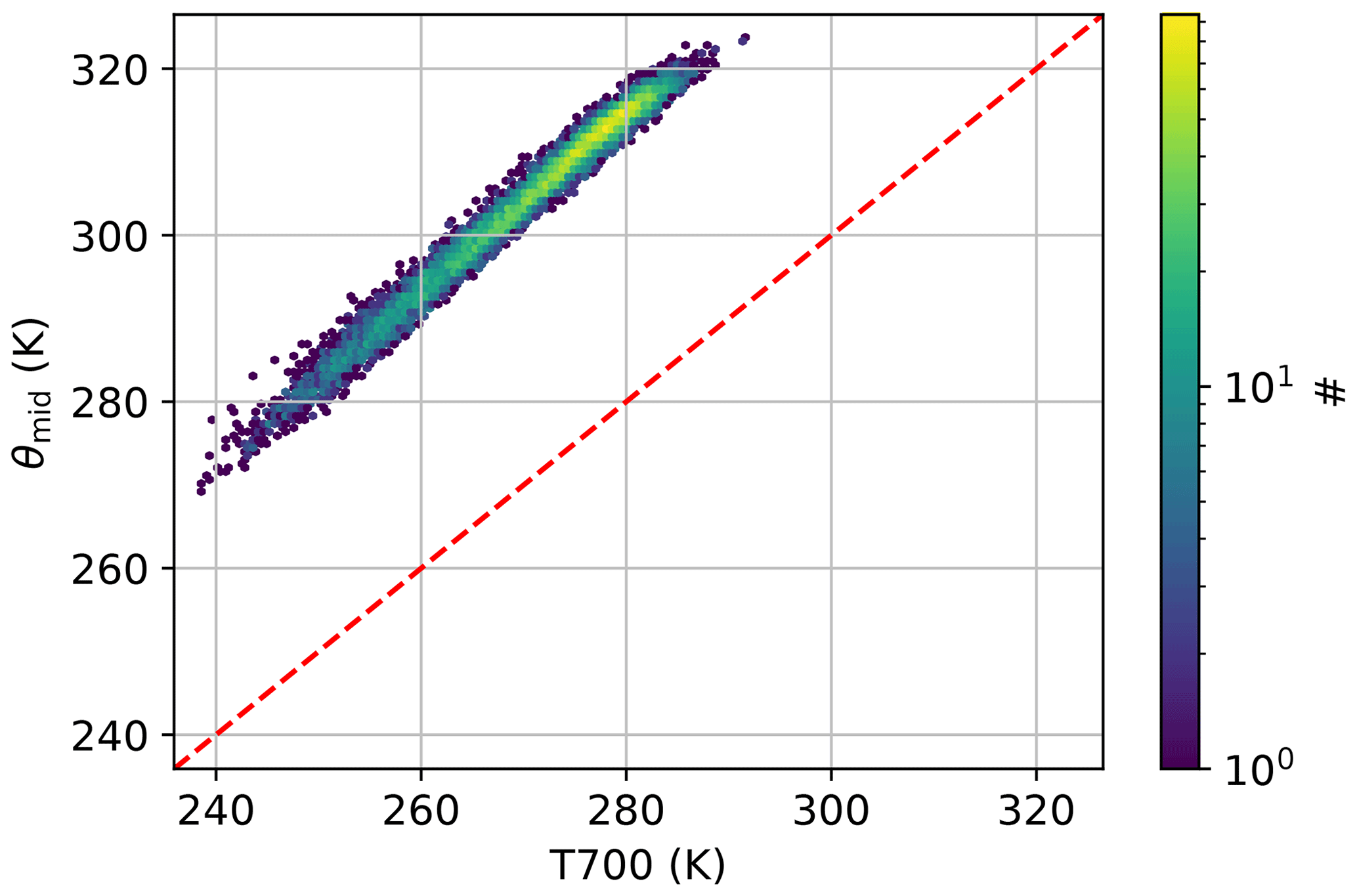
Figure 12A heat map of the relationship between θmid and T700, taken from the Park Falls TCCON data. The dashed red line denotes the 1:1 line.

Figure 13ADCFs derived from 2-month periods from 18 sites throughout the TCCON network versus mean potential temperature between 500 and 700 hPa over the same 2-month period. Each panel is one of the TCCON CH4 windows. The text inset in each panel gives the intercept and slope of the robust fit through the data shown by the dashed black line.
The magnitude of this temperature dependence varies from gas to gas: the primary TCCON CO2 windows have almost no slope, while the N2O windows have slopes of ADCF vs. θmid that are similar to or larger than the CH4 5938 window. We plan to investigate these temperature dependence behaviors more thoroughly in the next major GGG version and to identify spectroscopic improvements that will reduce or eliminate this behavior using a similar approach to that described for O2 in Sect. 6.3.
8.1.3 Fitting windows excluded in GGG2020
Based on the ADCF analysis, several spectral windows were excluded from the TCCON GGG2020 product. Figure 14 shows the ADCF versus θmid plots for two CO windows and two weak CO2 windows. The CO window centered at 4233 cm−1 (Fig. 14a) has a slightly stronger temperature dependence and a clearly larger scatter than the 4290 cm−1 CO window (Fig. 14b). We suspect this is due to water interference; the 4233 cm−1 CO window has more water lines in it than the 4290 cm−1 window. We examined the spectral residuals in both CO windows to try to identify and correct the water interference but were not able to reduce it to satisfactory levels. Thus, in GGG2020, the XCO product relies on only the 4290 cm−1 window.

Figure 14Similar to Fig. 13, except for two CO windows (a, b) and two weak CO2 windows (c, d).
Similarly, the new product was planned to use two windows, one centered at 6073 cm−1 and another at 6500 cm−1. However, as shown in Fig. 14c and d, the 6500 cm−1 window's ADCF has more scatter and a stronger temperature dependence than those of the 6073 cm−1 window. As the 6500 cm−1 also has more water interference than the 6073 cm−1 window, we elected to use only the 6073 cm−1 window.
Lastly, we also removed a number of HCl windows. TCCON instruments use HCl lines to assess instrument alignment with an HCl cell that can be illuminated by the solar beam or an internal lamp. TCCON used 16 windows to measure HCl in GGG2014, but like the CO and wCO2 windows, many of these have water absorption lines in them. We can diagnose unaccounted-for water interference by computing the ADCFs for each HCl window from Darwin 2015 data, split by the amount of water in the column. The result is shown in Fig. 15. Most of the GGG2014 windows have a clear difference in ADCF, with small or large water column amounts. Based on this, we chose to only retain the 5625, 5687, 5702, 5735, and 5739 cm−1 windows. Most of the windows removed clearly have a water interference. The 5754 and 5763 cm−1 windows are special cases. The 5754 cm−1 window was rejected because its air mass dependence is slightly more negative than the retained windows. The 5763 cm−1 window was rejected because it exhibits a clear temperature dependence in the window-to-window scale factors (Sect. 8.2).
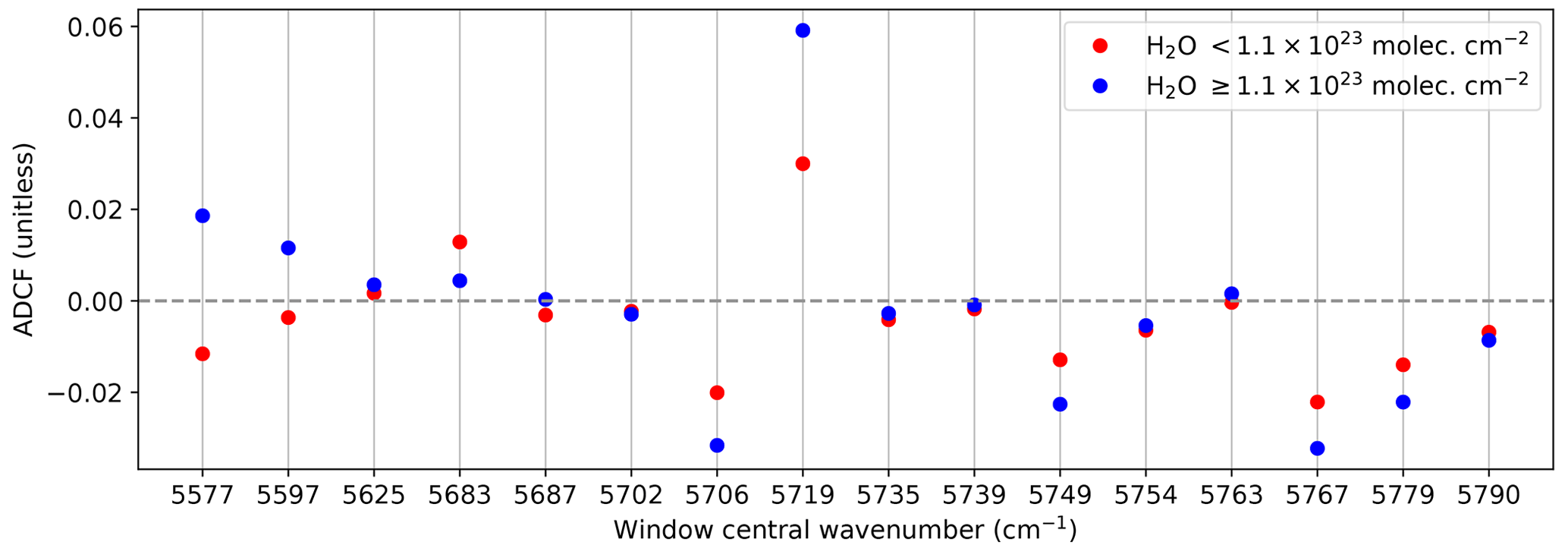
Figure 15ADCF calculated for each HCl window from 2015 Darwin data for two data subsets with different amounts of water in the atmosphere.
8.2 Updated window-to-window averaging
Many gases retrieved by GGG are retrieved in more than one spectral window. GGG retrieves the column amount in each window separately then averages together the columns with similar averaging kernels to produce a mean value. Specifically,
where subscript j represents the spectral window. That is, the average value for the ith measurement () is an error-weighted average of the individual windows' column amounts (yij, with errors ϵij), with a mean bias in each window removed by the per-window scale factor sj. The errors ϵij are the posterior errors in the Xgas amounts as calculated from the spectral residuals.
In GGG2014, the sj values were determined online using an iterative process that minimizes the differences between yij and the corresponding values. While this calculates sj values that best fit the data being averaged, it means that how the windows are combined depends on how many data are averaged at once – processing a month could give different results than processing a year of data, for example. Thus, while GGG2020 retains the capability to compute the sj values on the fly, the sj values are prescribed for standard TCCON processing, and all sites use the same sj values.
To determine the standard TCCON sj values, we used a very similar approach to how we derived the ADCFs in Sect. 8.1. Specifically, we calculated the sj values for 2-month subsets of data from the same 18 TCCON sites as in Sect. 8.1 and fit these values versus θmid. As with the ADCFs, we used the values of the fit at θmid=310 K as the final choices of sj.
8.3 Updated in situ bias correction
As in GGG2014, the GGG2020 , , , and products are tied to standard scales by in situ aircraft, balloon, and/or radiosonde measurements to remove any mean multiplicative bias introduced by error in absorption line intensity. As the absorption of a gas is the product of its column density and spectroscopic cross-section, a bias in the mean line intensity (and therefore the cross-section) will by definition lead to a multiplicative bias in the simulated absorption and thus the retrieved column density. Unlike GGG2014, XCO in GGG2020 is not tied to in situ measurements due to previous work that found that the difference between TCCON XCO and both NDACC (Kiel et al., 2016a) and MOPITT (Hedelius et al., 2019) XCO was approximately the magnitude of the in situ correction. Those analyses suggest that the GGG2014 7 % CO scaling was likely to be spurious. However, we do evaluate XCO against a subset of in situ data from AirCore below.
Comparison of TCCON data against in situ data follows the following steps:
-
Identify in situ vertical profiles in available data and convert to a standardized file format.
-
Extend the profiles' tops to 70 km altitude using the standard GGG2020 priors (shown in Laughner et al. (2023) to have good agreement with in situ profiles in the stratosphere) and to the surface by extrapolation or use of surface data.
-
Match profiles to available TCCON spectra.
-
Run custom retrievals using the matched profiles as the a priori trace gas profile.
-
Compare integrated in situ Xgas values against matched TCCON data, accounting for TCCON vertical sensitivity.
Points 1–4 are described in detail in Appendix C. Briefly, we use profiles from
-
the GLOBALVIEWplus 5.0 CO2 (Cooperative Global Atmospheric Data Integration Project, 2019) and GLOBALVIEWplus 2.0 CH4 ObsPack (Cooperative Global Atmospheric Data Integration Project, 2020) products;
-
AirCore balloon measurements (Tans, 2009; Karion et al., 2010) flown by NOAA (v20201223, Baier et al., 2021) at multiple TCCON sites and by FMI/LSCE/RUG at the Sodankylä, Finland (Kivi and Heikkinen, 2016), and Nicosia, Cyprus, TCCON sites;
-
the Infrastructure for Measurement of the European Carbon Cycle (IMECC) campaign;
-
Profiles over the Manaus, Brazil, TCCON site (Dubey et al., 2016);
-
ARM radiosondes over the Darwin, Australia (Deutscher et al., 2010), and Lamont, OK, USA, TCCON sites.
CH4 profiles have an additional correction to the stratospheric levels obtained from the GGG2020 priors; see Sect. C3 for details. We have addressed the recent change in CO2 data from the X2007 to X2019 WMO scales, which will be covered in Sect. 8.3.2. Due to the relative sparsity of N2O profiles, GGG2020 TCCON N2O products were evaluated against surface N2O data and using a different approach, which will be covered in Sect. 8.3.3. The number of usable profiles for each gas is given in Table 4.
The use of ObsPack data represents a slight methodological change compared to GGG2014. Most of the in situ aircraft profiles used for the GGG2014 in situ correction are included in the ObsPack, and switching to the ObsPack instead of individual campaigns' data files will allow us to use the same tools to ingest future new profiles added to the ObsPack. This also allows us to benefit from the data curation and quality control efforts of the ObsPack team. With the larger number of profiles now available (especially for CO2), we are able to test for correlations with potential sources or metrics of bias. However, the primary purpose of the in situ comparison remains to tie TCCON (and, through TCCON, satellite) GHG data to the same metrological scales as in situ GHG data.
8.3.1 CO2, CH4, CO, and H2O in situ comparisons
The first step in comparing TCCON , , XCO, or to their respective in situ profiles is to match each in situ profile to temporally proximate, good-quality TCCON retrievals. For this step, we define custom quality filters. A TCCON retrieval is considered to be good quality in this context if it fulfills the following criteria:
-
Fractional variation in solar intensity (FVSI) is ≤0.05. This is the standard deviation of solar intensity divided by the average solar intensity during the ∼80 s long scan, and it filters out observations impacted by intermittent clouds.
-
Solar zenith angle (SZA) is ≤80°. This avoids observations at large air masses, where spectroscopic errors can be more pronounced.
-
The unscaled Xgas value is >0 mol mol−1. A negative retrieved value is unphysical, and the distribution of retrieved values should not be large enough to make negative values a reasonable part of it.
-
The Xgas error is <2ϵmedian, where ϵmedian is the median error for that Xgas across all the spectra used for the given gas. This restricts us to observations where the observed spectra were fit reasonably well.
-
The median Xluft (see Eq. 4) for a comparison is between 0.996 and 1.002. Xluft and this rational are explained near the end of this subsection.
For each in situ profile, we require at least 30 TCCON observations (each ∼80 s) to pass these quality checks within a certain window of time around the corresponding profile's lowest altitude measurement. Our initial window is ±1 h. If 30 points meeting these criteria are not present within ±1 h, we increase both the time window and the allowed Xgas error, trying the combinations (±1 h, <2ϵmedian), (±2 h, <3ϵmedian), and (±3 h, <4ϵmedian). We use the smallest of these time and error windows that yield 30 passing TCCON observations, but if a profile does not have 30 passing TCCON observations in the (±3 h, <4ϵmedian) range, it is removed from the comparison.
The remaining in situ profiles are integrated following Wunch et al. (2010), where the integrated in situ Xgas value is calculated as follows:
where
-
p is the vector of pressure at each profile level;
-
is the vector of water dry mole fractions at each profile level;
-
γxa is the TCCON posterior profile (i.e., the prior times the retrieved VMR scale factor γ);
-
δx is the difference between the in situ (xinsitu,i) and TCCON posterior (xa,i) profiles, modified by the TCCON averaging kernel (ai) ().
I represents the pressure-weighted integration function:
where
-
dpi represents the pressure thickness of layer i;
-
gi represents the acceleration from gravity at layer i;
-
Mair and represent the mean molecular masses of dry air and water, respectively.
The integrated in situ Xgas values are compared against the median of the TCCON Xgas values from the matched observations. The TCCON Xgas values used here have the air mass correction (Sect. 8.1) and window-to-window averaging (Sect. 8.2) applied. Because we expect the bias in the TCCON data to arise from incorrect absorption line strengths or broadening coefficients, it should be a multiplicative bias. Therefore, we calculate an uncertainty-weighted mean of the TCCON in situ Xgas values to derive the bias correction. We consider five sources of uncertainty:
-
measurement error in the in situ data
-
uncertainty from the unmeasured portion of the free troposphere (will be zero if the in situ vertical profile extends through the tropopause)
-
uncertainty from the unmeasured portion of the stratosphere
-
random error in the TCCON observations
-
bias in the TCCON observations from instrument misalignment or similar hardware concerns.
The calculation of each term and how they are combined for the error bars in Fig. 16 are detailed in Appendix C6.
The results of the TCCON–in situ comparison are shown in Fig. 16. In this plot, the y axes are the ratio of TCCON to in situ Xgas amounts, and the x axes show Xluft (see Eq. 4 in Sect. 6.3 for the definition). We will return to the significance of Xluft shortly. The use of TCCON in situ ratios to derive the in situ correction is equivalent to the best-fit lines forced through the origin used in Wunch et al. (2010) as the best-fit line through the origin is essentially the mean TCCON in situ ratio. As in Wunch et al. (2010), a ratio (or slope in Wunch et al. (2010)) >1 indicates that TCCON Xgas values are biased high relative to in situ and vice versa for ratios <1. The use of ratios directly in Fig. 16 allows us to more clearly identify outliers and evaluate the correlation of the TCCON vs. in situ bias with other variables, such as Xluft here.
The ratios from Fig. 16 indicate that the mean biases are within approximately 1 % of unity in all cases, with water being the furthest from unity at 0.9883 (−1.17 %). The differences among the CO2 products are interesting; the standard CO2 product is biased about 1 % high before correction (which is in line with expected uncertainties for the CO2 lines), while the other two CO2 products are much closer to unity (0.08 % for wCO2 and 0.14 % for lCO2). This suggests that the absorption coefficients in these latter two windows are more accurate than in the standard TCCON windows (which are centered at 6220 and 6339 cm−1). However, as the wCO2 and lCO2 are more sensitive to the upper and near-surface atmosphere, respectively, it may be that this reflects other factors, such as the accuracy of the a priori temperatures at those levels.
Additionally, we note that the TCCON product changed from being 1 % low compared to in situ (pre-in situ correction) in Wunch et al. (2015) to 1 % high here. We would expect this to be due to changes in spectroscopy, such as an average decrease in CO2 line strengths or an increase in O2 line strengths. However, we are in the process of conducting a full attribution study for all the component changes between GGG2014 and GGG2020 and will reserve a final conclusion until that is complete.
The CO comparison (Fig. 16e) suggests that, without scaling, the GGG2020 XCO has no significant bias with respect to AirCore CO measurements. Figure 16e shows significant variation in the TCCON in situ CO agreement, with individual points also having large uncertainty. This resulting 2σ uncertainty in the mean ratio is significantly larger than for the other gases at 0.0526. Thus, the mean TCCON in situ CO ratio is well within its 2σ uncertainty of 1. We do acknowledge that limiting the CO comparisons to AirCore profiles alone may contribute to a larger uncertainty than if aircraft campaigns were included due to the use of a CO-spiked fill gas in AirCores (see Sect. 2.1 of Martínez-Alonso et al., 2022). However, comparing TCCON XCO to AirCore profiles was significantly more straightforward than including aircraft profiles since the already-matched AirCore profiles for CO2 and CH4 intrinsically include CO as well. Given the other reasons discussed above for not applying an in situ-derived scaling to GGG2020 XCO or the process needed to match aircraft data with TCCON (see Appendix C1.1), we chose to accept the additional uncertainty from using AirCore profiles only. Future versions of the TCCON data product will re-evaluate the inclusion of aircraft profiles alongside AirCore ones.

Figure 16Plots of the TCCON in situ Xgas ratios for (a) CO2, (b) wCO2, (c) lCO2, (d) CH4, (e) CO, and (f) H2O. In all plots, the y axis is the ratio of TCCON in situ Xgas, and the x axis is the median Xluft value for the TCCON observations in a comparison (see text for explanation of Xluft). The marker style of each comparison indicates the source of the in situ data, and the color indicates which TCCON site the comparison occurred at. The text inset in the lower-right corner of each plot gives the uncertainty-weighted mean TCCON in situ ratio and its 2σ uncertainty. The dashed black lines mark the mean ratio. Panels (a), (b), and (c) are set to use the same y limits; some of the error bars in (b) go outside the y limits.
Figure 16 also provides insight into how instrumental errors affect different TCCON products. Under ideal circumstances, Xluft (the quantity on the x axis) should be 1; in practice, the nominal value for the TCCON network is 0.999 due to small residual biases in the O2 spectroscopy. Deviations of Xluft from the nominal value indicate either (a) variable errors in spectroscopy, such as temperature or pressure broadening, or (b) instrument issues, such as a misalignment in the beam path. From Fig. 16a, we can see that the TCCON in situ ratio tends to be less when Xluft<0.999 and greater when Xluft>0.999. The slope for Fig. 16a is 0.363. This translates to a bias in CO2 of about 0.15 %, or approximately 0.5 ppm, when Xluft is 0.004 units away from the nominal value of 0.999 (). To keep this bias well below the expected 0.25 % accuracy, we limit the comparison used here to those cases where Xluft is between 0.996 and 1.002 and have instituted additional quality checks of TCCON data that filter out observations when Xluft is outside the range of 0.995 to 1.003 for an extended period of time. Additionally, Xluft is now reported in the public data set alongside other Xgas retrievals.
We note that the standard CO2 and the near-surface-sensitive lCO2 products show the clearest dependence on Xluft. The reason for this is not clear at this time, though it implies a stronger dependence of these products on ILS compared to the other four products discussed in this section. Future versions of GGG are planned to account for errors in the ILS, which we hope will mitigate this bias and improve the accuracy of CO2 data when Xluft is outside the 0.995 to 1.003 range.
The correlation of and with Xluft implies that we could develop an Xluft-based bias correction for those CO2 products. Such a correction is planned for a minor update to the GGG data product. Our aim is to quantify the underlying physical drivers of the bias and use the correlation of those factors with Xluft to derive the bias correction. This would allow us to use the comparison to in situ data shown here as an independent verification of the bias correction's efficacy.
8.3.2 Addressing the CO2 scale change from X2007 to X2019 and changing O2 dry mole fraction
The update from the previous WMO CO2 X2007 calibration scale to the new X2019 calibration scale (Hall et al., 2021) occurred late enough in the process of releasing GGG2020 that we were not able to incorporate it into the initial release. Given the clear need expressed by the community to have TCCON data tied to the same scale as in situ data, we have since derived new in situ correction factors to tie all three TCCON products to the X2019 scale. Doing so required obtaining in situ data that had been adjusted to the new scale, which we did in one of three ways:
-
The preferred approach was for the data originator to fully recalibrate their data to the new scale using the updated standards provided by the NOAA Global Monitoring Laboratory. NOAA AirCore and some NOAA ObsPack data (GLOBALVIEWplus v7, Schuldt et al., 2021) followed this approach.4
-
The second approach was for the data originator or an intermediate provider to adjust the CO2 data using the linear correction described in Sect. 9.1 of Hall et al. (2021). The remaining NOAA ObsPack data not covered by approach no. 1 followed this approach.
-
The third approach was for us to perform the same linear correction as no. 2 ourselves. All other data used this approach.
Also recall that the profiles must be extended to 70 km altitude using the TCCON standard priors to ensure that the same vertical extent is captured in the in situ and TCCON column averages. As discussed in Laughner et al. (2023), the standard priors are derived from NOAA data at the Mauna Loa and American Samoa observatories and so are also intrinsically tied to WMO calibration scales. To ensure consistency throughout the in situ profiles, we used the latest available monthly average CO2 flask data on the X2019 scale as input to the priors when generating the profile extensions. Once this was complete, we redid the analysis described in Sect. 8.3 with the in situ profiles adjusted to the X2019 scale to generate updated correction factors.
The overall effect of the scale change for each of the three TCCON CO2 products is shown in Fig. 17 compared to the “raw”, non-bias-corrected value on the x axis. The magnitude is about +0.15 ppm for typical current values of 400 ppm. In the TCCON data products, there are three CO2 variables with the suffix _x2019 which are adjusted to the new X2019 scale.
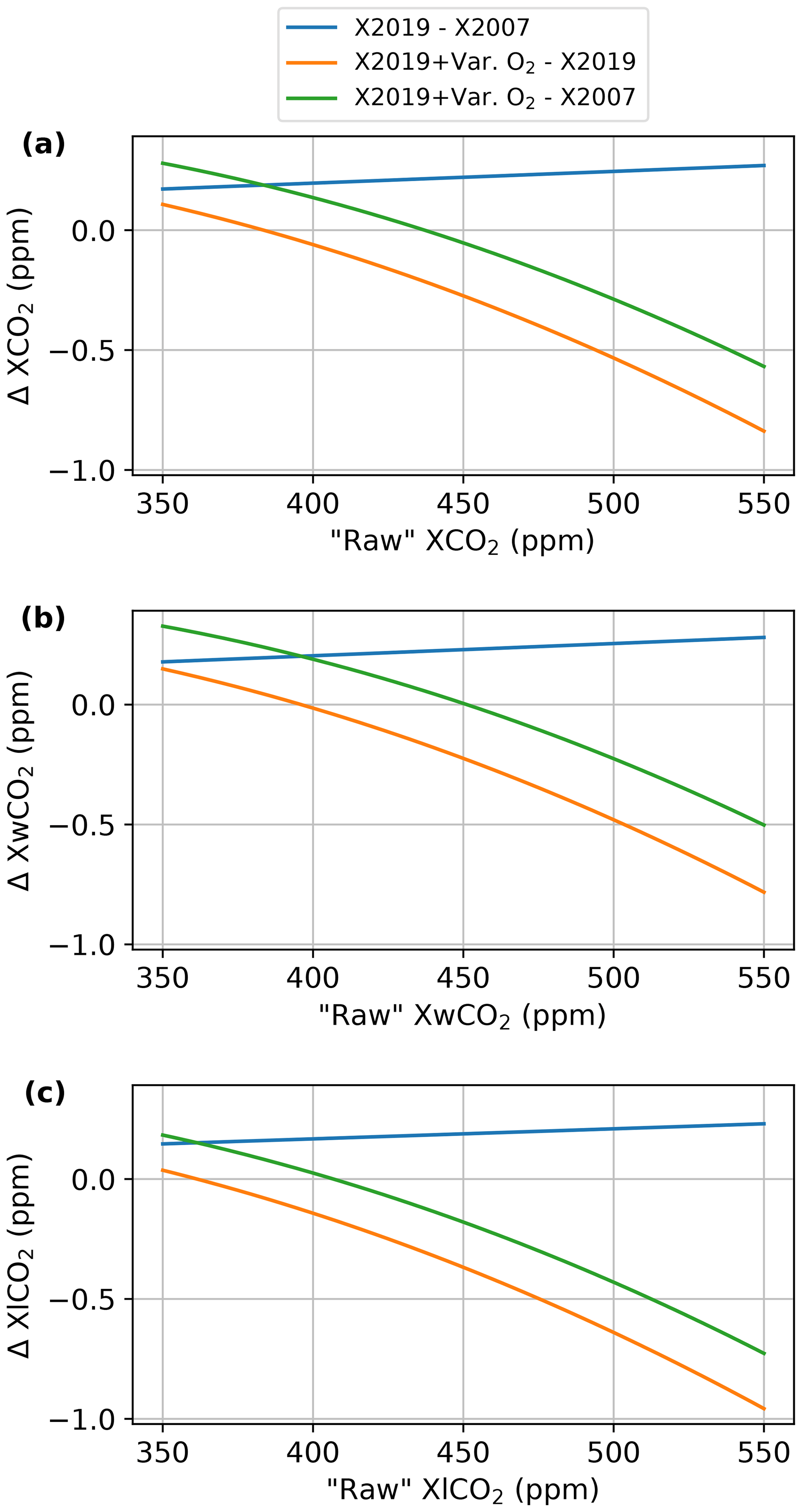
Figure 17The change in TCCON (a) , (b) , and (c) due to the WMO scale change, the change in assumed O2 dry mole fraction, and the combination of both. The x axis is the raw value that has no in situ bias correction and assumes a fixed O2 dry mole fraction. The “X2019–X2007” line shows the difference due to only the CO2 WMO scale change, the “X2019+Var O2–X2019” shows the difference due to only the change from fixed to variable O2 dry mole fraction, and the “X2019+Var. O2–X2007” line shows the total change from both effects combined.
Another source of bias that is of similar magnitude to the effect of the scale change is the assumed O2 dry mole fraction. As shown in Eq. 1, the column-average dry mole fractions reported by TCCON are computed by dividing the column density of the target gas by the O2 column density and scaling by the mean O2 dry mole fraction in the atmosphere. We have assumed that this dry mole fraction is fixed for the initial GGG2020 data products; however, it is in fact changing over time due to various processes, predominantly fossil fuel combustion and the land biosphere (Keeling et al., 1998; Keeling and Manning, 2014).
Because the effect of ignoring the change in the global average O2 dry mole fraction is of similar magnitude to the X2007 to X2019 scale change, we decided to account for the change in O2 dry mole fraction over time in the CO2 products updated to the X2019 scale. We did not retroactively apply this correction to the X2007 or the other Xgas products as doing so would change the Xgas values and require a new data version. This correction will be applied to all Xgas values in the next GGG data version.
Our approach to account for changing O2 dry mole fraction takes advantage of the anticorrelation between atmospheric O2 and CO2 to derive the O2 dry mole fraction from CO2 measured by TCCON. For our application, this assumption is sufficiently accurate; however, we note that this is not generally true for other applications of O2 N2 ratio data. Specifically, the value for in Eq. (1) is calculated as follows (see Appendix E1 for the full derivation):
where
-
, i.e., the change in the number of moles of O2 in the atmosphere for a given change in the number of moles of CO2 in the atmosphere. The choice of comes from the agreement with the measured change in as shown in Fig. 18. This value is chosen to remove the effect of long-term trends in the O2 dry mole fraction and ignores synoptic-scale variations due to, e.g., photosynthesis or fossil fuel emissions.
-
is the reference value for the dry mole fraction of O2. We use 0.209341 based on the value measured by Aoki et al. (2019) at Hateruma Island, Japan, in 2015 and adjust by ∼2 ppm to approximate the global mean by using the difference between the annual mean CO2 reported for Hateruma Island by Aoki et al. (2019) and that for the NOAA global marine boundary layer reference. A revised calculation accounting for the possible influence of fossil fuel emissions on Hateruma Island puts the global mean O2 dry mole fraction closer to 0.209347; however, the 0.209341 value is what is used in GGG2020.
-
is a reference value for the column-average dry mole fraction of CO2. We use (400 ppm) to approximate the value seen in TCCON data during 2015 (the same year as the value), though, as discussed below, it is not crucial that the O2 and CO2 reference values be for exactly the same time.
-
is the raw measured TCCON with air mass correction and assuming .
To validate this approach, we also compute the change in (including the effect of CO2 dilution) using data measured by the Scripps Institution of Oceanography at Alert, NWT, Canada (station code ALT); La Jolla Pier, California, USA (LJO); and Cape Grim, Australia (CGO), as well as NOAA CO2 annual trend data (Lan et al., 2023). To approximate a global mean value, we follow Sect. 5.15.4.2 of Keeling and Manning (2014) and combine the data from these stations as (ALT + LJO)/4 + CGO/2.
The results of this comparison are shown in Fig. 18. The black line shows the change in computed using the Scripps data (see Appendix E2 for the methodology), while the other three lines represent calculated with Eq. (12) and various values of α. We can see that Eq. (12) with gives quite good agreement with the change in computed using the Scripps and NOAA global CO2 data.
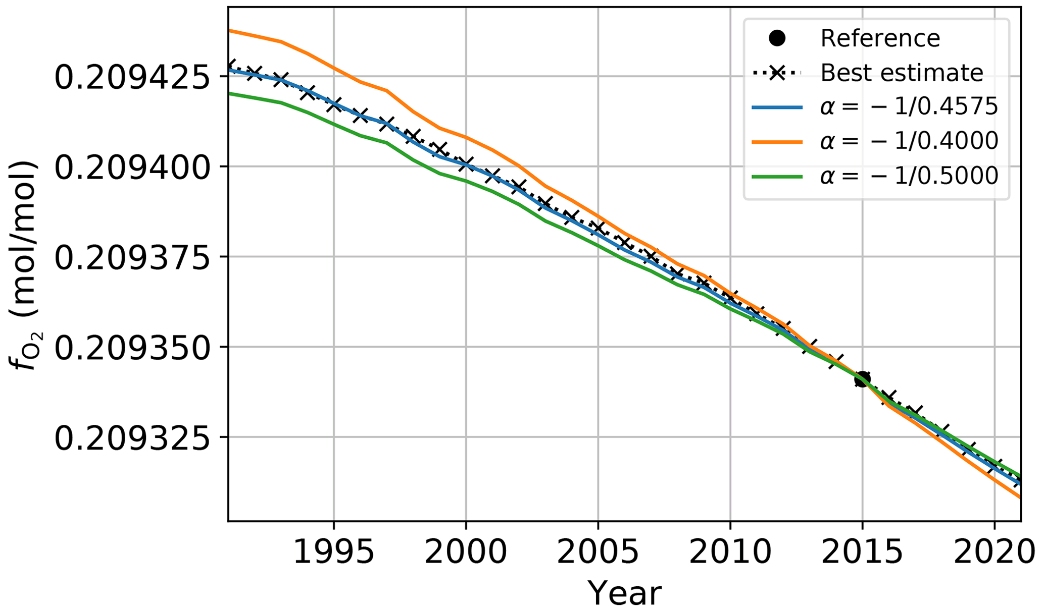
Figure 18Comparison of values calculated using Eq. (12) for three different values of α versus a best estimate of using from the Scripps Institute of Oceanography (Scripps O2 Program, 2022) and NOAA global mean CO2 (Lan et al., 2023) data. The three colored lines also use NOAA global mean CO2 data for the and values in Eq. (12). The black circle marks our reference value of .
The final step in adopting the variable O2 dry mole fraction was to recompute the in situ correction factor once more using the variable O2 dry mole fraction in the TCCON Xgas values for the comparison. Doing so ensures that any constant multiplicative bias introduced by incorrect or inconsistent values for the or values is scaled out. This is why, in the discussion above about the choice of those reference values, we note that it is not critical to have the O2 and CO2 reference values be exactly consistent.
The orange lines in Fig. 17 show the effects of the change from a fixed O2 dry mole fraction to the variable one. For values around 400 ppm, the change is of similar magnitude to the WMO scale change for CO2 products. If CO2 mixing ratios continue to increase in the future, the difference between using the incorrectly fixed and correctly varying O2 dry mole fraction would increase to 0.75 to 1 ppm in magnitude.
The green lines in Fig. 17 show the combined effect of the CO2 calibration scale change and the switch to a variable O2 dry mole fraction. For low raw values (i.e., values without the in situ bias correction and using a fixed O2 dry mole fraction), the two effects reinforce each other, but as the raw increases, the O2 dry mole fraction change starts to counteract part of the CO2 scale change.
, , and on the X2019 scale and accounting for the variable O2 dry mole fraction are now available in the public data set as variables xco2_x2019, xwco2_experimental_x2019, and xlco2_experimental_x2019. Users comparing to other data or model simulations and/or assimilations on the X2019 scale should use these variables. Anyone needing to compare against data still on the X2007 scale can use xco2, xwco2_experimental, and xlco2_experimental instead.
8.3.3 N2O in situ comparisons
To derive an in situ correction for N2O, we adopted a different approach than for the other gases due to the small number of N2O profiles over TCCON sites which our matching algorithm found in the NOAA CCGG Aircraft Program v1.0 ObsPack (Sweeney et al., 2018). Figure 19a shows the 10 profiles identified from the ObsPack, and Fig. 19b shows the TCCON in situ ratio vs. Xluft relationship for these profiles. We note that this scarcity of profiles was partly due to the criteria used to filter for good-quality profiles (Appendix C1.1). However, given how well mixed N2O is in the troposphere, the criteria intended to ensure enough vertical resolution to capture plumes of CO2 or CH4 could be relaxed for N2O in future TCCON in situ comparisons to increase the number of available N2O profiles for comparison.
The available profiles were further restricted by our criteria for coincidence with good-quality TCCON observations; 2 of these 10 profiles do not meet the coincidence criteria for inclusion in Fig. 19b, and 5 of the remaining 8 fall outside the allowed Xluft range of 0.996 to 1.002. With the available data, it is difficult to distinguish whether there is significant correlation between Xluft and TCCON bias and therefore whether those 5 comparisons below Xluft=0.996 should be excluded. As their exclusion would significantly alter the in situ correction for , we tested a second approach to derive the N2O correction.

Figure 19(a) The available N2O profiles over TCCON sites from the NOAA CCGG Aircraft Program v1.0 ObsPack (Sweeney et al., 2018). (b) TCCON in situ ratio vs. Xluft, similarly to Fig. 16 but for N2O. (c) The TCCON in situ ratio derived using surface NOAA N2O data versus mid-tropospheric potential temperature. The dashed gray line is a robust fit to the data. The text in the lower-right-hand corner gives the mean TCCON in situ ratio (denoted also by the horizontal dashed black line) and its 2σ standard deviation. The points are colored by TCCON site.
This alternate approach uses NOAA surface N2O data from the NOAA Halocarbons and other Atmospheric Trace Species (HATS) program (Dutton et al., 2023) combined with the GGG2020 priors to generate pseudo-in situ profiles. This takes advantage of the limited vertical variation in N2O up to the tropopause seen in Fig. 19a and the good accuracy of the GGG2020 priors in the stratosphere (Laughner et al., 2023). These pseudo-in situ profiles use the HATS N2O data for the tropospheric VMRs, the GGG2020 priors for VMRs above 380 K potential temperature, and linearly interpolates in between. These pseudo-in situ profiles are then integrated following Eq. (10) to produce a pseudo-in situ and are compared to TCCON in the same manner as the other gases. As we are not limited by when an aircraft provided an N2O profile over a TCCON site, we can compare to TCCON observations from any time. We use spectra from the same sites and days as the other gases, filtered for the following criteria:
-
FVSI ≤0.05, as for the other gases;
-
Xluft between 0.996 and 1.002, as for the other gases;
-
the difference between prior HF column density and retrieved HF column density is molec. cm−2.
The filtering on the HF column helps to remove cases where the N2O stratospheric prior used in the pseudo-in situ profiles is incorrect. HF is a gas found almost exclusively in the stratosphere, and in GGG2020, the HF and N2O stratospheric priors are coupled. Thus, when the retrieved HF column is substantially different from the prior, that indicates that the HF prior was incorrect, which implies the same for the N2O profile. HF columns tend to be between 1 and 2×10¹⁵ molec. cm−2; thus, 2×10¹⁴ molec. cm−2 represents a 10 % to 20 % error in the HF prior. Given that the stratosphere component of N2O is <20 % of the column, and assuming that the percent error in the N2O prior is similar, this keeps the random error in the pseudo-in situ to less that 2 % to 4 %. All together, these filtering criteria retain approximately 8600 TCCON observations from the initial set of observations used in the in situ correction analysis.
This larger sample set for N2O allowed us to identify a correlation in bias with atmospheric temperature. Figure 19c shows how the TCCON in situ ratio varies with potential temperature at 700 hPa. As in the ADCF analysis (Sect. 8.1), these potential temperature values come from the GEOS FP-IT meteorology used as input to the GGG retrievals. The presence of this bias suggests that there is an error in the temperature dependence of the N2O cross-sections (similar to that we identified and removed for O2, Sect. 6.3). In the near term, within 2–3 years, we plan to develop a post-processing correction for this temperature bias in N2O for inclusion in a minor update to the TCCON GGG2020 data. Long term, the underlying error in the spectroscopic model will be corrected so that the next major TCCON data release will have improved data.
For GGG2020, we elected to choose the in situ correction as the value of the fit in Fig. 19c at 310 K potential temperature. This is consistent with the choice of ADCF values at the same temperature (Sect. 8.1). The value of 0.9822 is very close to the mean TCCON in situ ratio using the eight true in situ profiles in Fig. 19b. That both methods agree gives us confidence that this is a reasonable value to use for the in situ correction. We are also investigating applying the slope from Fig. 19c to TCCON as a temperature-based bias correction. Figure 20 demonstrates the difference this correction would make in comparison to both the in situ data (Fig. 20a, b) and the column-average dry mole fractions themselves (Fig. 20c).
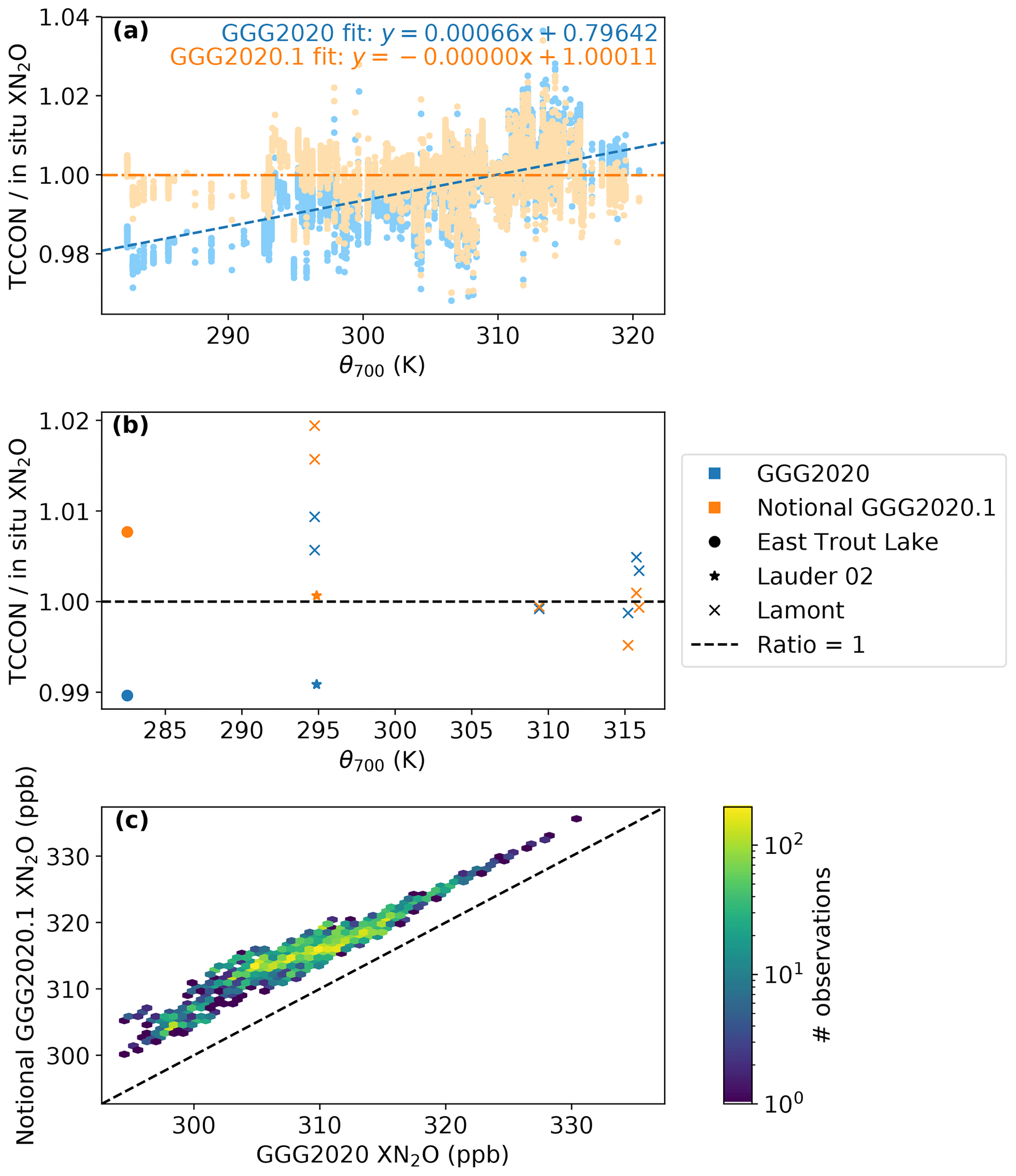
Figure 20Future correction for . (a) Similar to Fig. 19c except showing the ratio between TCCON and the surface-derived from GGG2020, with the in situ correction factor of 0.9821 applied in blue and the expected temperature-corrected in orange, along with their respective fits. (b) Similar to Fig. 19b but, like panel (a) of this figure, comparing the ratios of GGG2020 and temperature-corrected to in situ. (c) A 2D histogram comparing the current and notionally corrected .
8.3.4 In situ bias correction summary
A summary of the in situ correction factors, their errors, and what in situ calibration scales each product is tied to are given in Table 4. Because these correction factors are the mean TCCON in situ ratio, dividing the air-mass-corrected and window-averaged values by these correction factors removes the mean TCCON–in situ bias.
Table 4In situ correction factors and their errors for each Xgas product evaluated against in situ data. The “Calibration scale” column indicates which scale or source these data are tied to by the AICFs. The N column indicates how many profiles are used to calculate the AICF for that gas. The column indicates what O2 dry mole fraction was used in the conversion of column density to column-average dry mole fraction: “Fixed” means in Eq. (1), and “Var.” means that the variable dry mole fraction described in Sect. 8.3.2 was used. n/a – not applicable
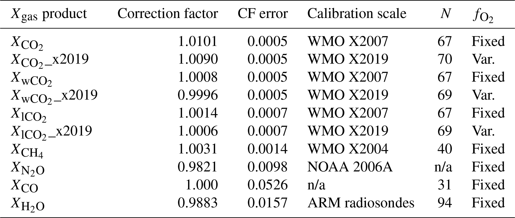
In the TCCON data, users will find two sets of variables. Those with the _x2019 suffix (xwco2_experimental_x2019, xlco2_experimental_x2019, and xco2_x2019) are those tied to the WMO X2019 CO2 scale and which use the variable O2 dry mole fraction. Those CO2 variables without the _x2019 suffix remain tied to the WMO X2007 CO2 scale and still use the fixed O2 dry mole fraction. All other gases (xch4, xco, etc.) also still use the fixed O2 dry mole fraction. Releasing the rescaled as new variables rather than creating a new TCCON data version with the existing variables rescaled was chosen for several reasons. First, it is logistically simpler, allowing us to provide this update more quickly. Second, during this transitional period when existing CO2 data are available on both the X2007 and X2019 scales, having both X2007 and X2019 allows users to switch back and forth easily if they need to match up with other data sets on a mix of both scales. Third, this approach provides for the release of more recent TCCON data without disrupting existing users' workflows – users do not have to worry about existing variables changing but can switch their analyses to use the updated variables if and when they wish. Incorporating the variable O2 dry mole fraction for all gases is planned for an upcoming minor revision of the TCCON data (tentatively called GGG2020.1). Likewise, a temperature-corrected product will be included in GGG2020.1 or the follow-on GGG2020.2, depending on development time.
To calculate an uncertainty in the GGG2020 data set, we selected three days from the East Trout Lake data set, spanning a range of atmospheric water vapor, surface temperature, and solar zenith angle (Fig. 21). Each known source of uncertainty is modeled or perturbed by a realistic amount in the GFIT forward model (the quantitative amounts are described in the following paragraphs), and we compute the percent fractional difference in Xgas between the perturbed and unperturbed values. The total uncertainty is computed as the sum in quadrature of the individual uncertainties. For each gas, we have plotted the contributions of each source as a function of solar zenith angle for the date of 11 June 2019 in Figs. 23–25. The same figures for cold, dry 18 February are in the Appendix in Figs. B1–B3, and the figures for warm, wet 23 July are in Figs. B4–B6. The sums in quadrature of all the sources of error for each gas are plotted together for the 3 stated days in Figs. 26–28. Each source of uncertainty included in our error budget is described below. Table 5 toward the end of this section summarizes the error budget for the primary TCCON products.
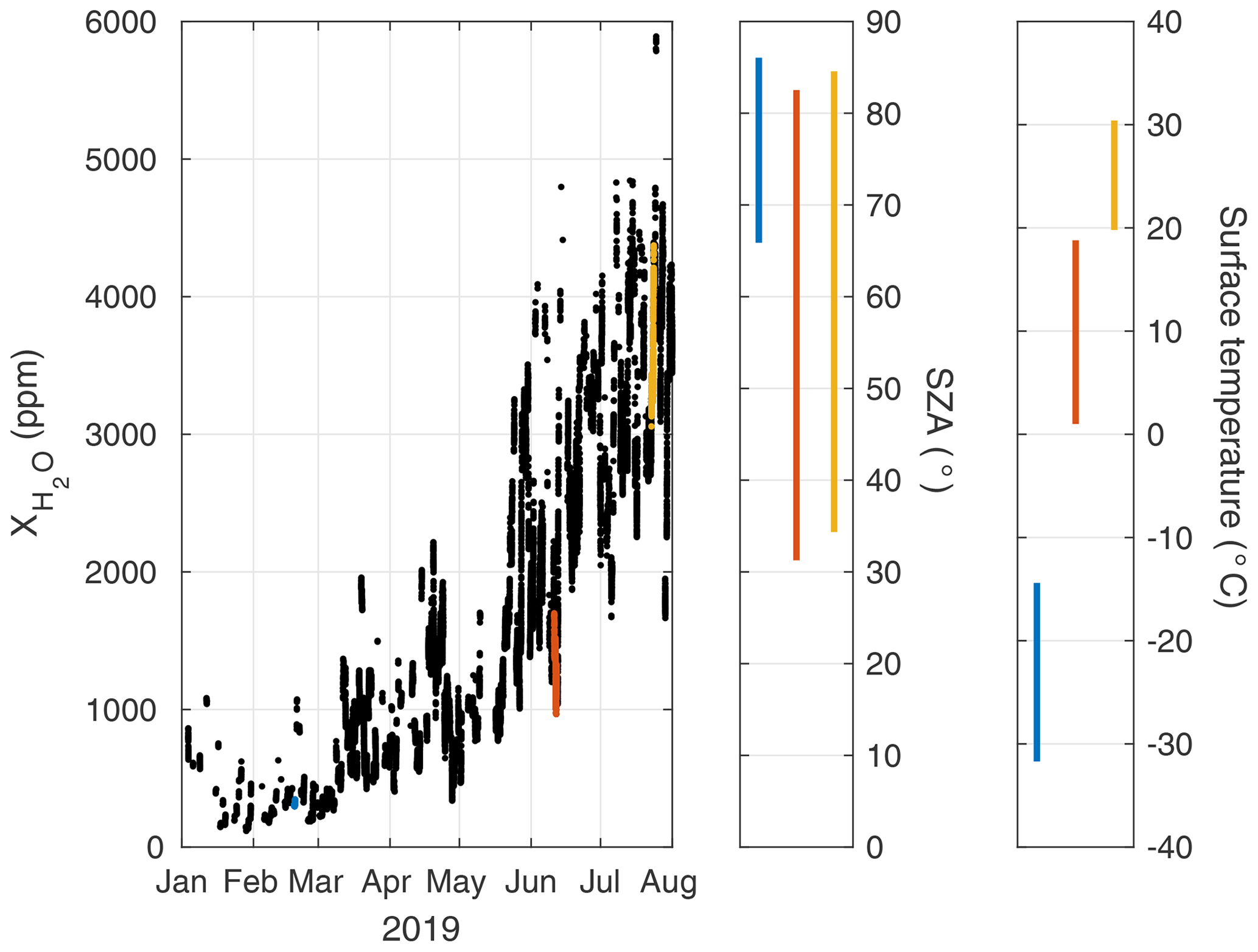
Figure 21The three dates chosen for the error budget calculations are from East Trout Lake on 18 February (blue), 11 June (red), and 23 July (yellow) 2019. These dates were chosen to span a range of water vapor, solar zenith angle, and surface temperature. In the left panel, the black data points show the full East Trout Lake record between January and August 2019 for reference.
9.1 Field of view
The field of view (FOV) is the maximum solid angle viewed by the detector element, and its value is set by the field stop diameter inside the instrument. It is an important parameter in the GFIT forward model because it defines the extent of off-axis rays that pass through the interferometer, ultimately limiting the spectral resolution of a spectrum. The field stop diameter is set by a physical pinhole that ranges from 0.5 to 1.3 mm and is drilled into a thin plate within the instrument, and its size can be in error by a few percent. Here, we increase FOV by 7 % to reflect any uncertainty in the field stop diameter.
9.2 Continuum basis functions
In GGG2020, the number of continuum basis functions has been optimized to improve the spectral fits without over-fitting the data (see Sect. 7). Here, we increase the number of continuum basis functions fitted by 1 in all windows that have widths >5 cm−1 to assess the sensitivity of our choice of the number of basis functions to the retrieved Xgas value. The gases excluded from this test because of their fitting-window widths are HF, HCl, and some H2O and HDO windows.
9.3 Solar pointing
The observer-sun Doppler stretch (OSDS) is a calculation made by GFIT based on the Earth–Sun radial velocity and the Earth's rotational velocity component under the assumption that the solar tracker is imaging the center of the Sun. It defines the Doppler stretch of the solar absorption lines relative to the telluric (atmospheric) absorption lines. If the solar tracker is not imaging the exact center of the Sun, the solar lines may be Doppler-shifted relative to the telluric lines, creating systematic residuals in the spectral fits. Here, we increase the OSDS by 2 ppm to assess the sensitivity of the retrievals to a small pointing error from the Doppler stretch component alone. This error affects carbon monoxide more than the other gases because, for every telluric CO line in the spectrum, there is also a solar CO absorption line beneath, making it difficult to distinguish solar from telluric CO absorption. In GGG2014 and previous versions, this was a particular problem because the pointing was assumed to be in the center of the solar disk. In GGG2020, however, the solar-gas stretches are now fitted, reducing the impact of an OSDS error on the CO retrievals (see Wunch et al., 2015, Fig. 13). A solar-gas stretch is when the solar absorption lines' frequencies have to be stretched due to unaccounted-for Doppler effects, e.g., pointing away from the center of the solar disk.
Solar tracker pointing offsets also affect the ray tracing in GFIT, causing errors in the air masses calculated for a given spectrum. This error impacts all gas retrievals but should mostly be canceled out in the ratio between the gas of interest and oxygen. It shows up most prominently in Xluft as that is not a ratio between two retrieve gas columns (see Sect. 6.3 and Eq. 4). Here, we add a 0.05° pointing offset (poff), which represents a pointing error of about 20 % of the solar radius.
9.4 Prior
We modify the priors in several ways to estimate the uncertainties caused by various errors in the a priori profiles.
-
A priori pressure profile (prior pressure). We multiplied the pressure at each atmospheric level in the prior by 1.002 to scale up the pressure by 0.2 % at all altitudes. For the HCl cell pressure error, we added 0.14 hPa (0.138 atm) to the cell pressure, following the “pessimistic” uncertainty budget in Hase et al. (2013, P3565). The purpose of the HCl cells will be described in Sect. 9.18.
-
A priori temperature profile (prior temperature). We added 1 K to each atmospheric level in the prior.
-
A priori profile shape (prior shift). We shifted the a priori profiles down by one atmospheric level. In GGG2014, we shifted the priors down by 1 km; thus, this is a slightly different approach, but the level spacing is about 1 km in altitude near the tropopause, where this shift is most important for well-mixed tropospheric gases like N2O and CH4 and for HF, a stratospheric gas. H2O and HDO are not shifted as part of this process but are modified in an independent test.
-
A priori boundary layer CO (prior CO enhanced). The GEOS FP-IT CO profiles are created using an old emission inventory and tend to significantly overestimate emissions in urban regions that have reduced their emissions over time (e.g., Los Angeles). However, because of the coarse spatial resolution of GEOS FP-IT, sites that are located near to an urban center can be affected by the urban enhancements in the model. We therefore add an additional test that affects only the CO error budget, in which we add 25 ppb to the altitudes below 2 km to estimate the uncertainty caused by the incorrect lower-atmosphere shape in the GGG2020 CO prior profiles.
-
A priori H2O and HDO (prior h2o/hdo). We modified the water and HDO profiles by reducing the values in the first 1 km by 50 %.
9.5 Surface pressure
The surface pressure measurements we collect as part of our on-site meteorological data are important for determining the bottom altitude when integrating the total columns. The largest surface pressure uncertainty permitted by the TCCON data protocol is 0.3 hPa, but we have seen these instruments drift by up to 1 hPa. Here, we add 1 hPa to the surface pressure (pout) to calculate the sensitivity of the retrievals to this error.
9.6 Nonlinearity
Detector nonlinearities, described in Sect. 4.1, cause a discrepancy between the low-resolution spectral envelope and the high-resolution spectral lines, resulting in an offset at zero in the spectrum. These zero-level offsets are most readily observed in regions of the spectrum where strong absorption lines absorb all the incident light (Abrams et al., 1994). Here, we add 0.001 (0.1 %) to the zero-level offset (ZLO) parameter in GFIT; this is a large ZLO observed in the network.
9.7 Instrument line shape
The instrument line shape (ILS) of a Fourier transform spectrometer quantifies the optical alignment of the instrument and is independent of the alignment of the solar image. The ILS is characterized by two parameters: the modulation efficiency and phase error. The modulation efficiency is the broadening or narrowing of the ideal spectral line width in the instrument, and the phase error is the asymmetrical component of the spectral line that is caused by the misalignment. It is not currently possible to model phase error within GFIT, but we can model imperfect modulation efficiency. The TCCON data protocol requires that the instrument modulation efficiencies must be within 5 % of a perfect alignment. The modulation efficiency of a perfectly aligned interferometer is defined as a value of 1.0 at all optical path differences, taking self-apodization into account, and therefore the maximum and minimum modulation efficiencies acceptable in the network are 1.05 and 0.95, respectively. Here, we model two cases: a “shear” misalignment, where the modulation efficiency of the spectrometer increases linearly to 1.05 as a function of optical path difference, and an “angular” misalignment, where the modulation efficiency drops linearly to 0.95 as a function of optical path difference. See Sect. 8 of Wunch et al., 2015 for more details on the mathematical forms for these misalignments. We confirmed the misalignment by passing synthetic spectra generated by GFIT with these misalignments through LINEFIT (v14.8, Hase et al., 1999), a program designed to assess instrument line shapes (see Fig. 22).
Because GGG2020 cannot model phase errors, these sensitivity studies are likely to underestimate the full effect of ILS errors, and therefore we include both the shear and angular misalignments in the sum.
9.8 Other sources of error
This error budget does not include radiometric noise or spectroscopic errors. We omit radiometric noise because Wunch et al. (2011) showed that random noise does not introduce a bias in because TCCON spectra have a high signal-to-noise ratio due to the direct-sun viewing geometry and the strength of our target gases' absorption lines. We omit spectroscopic errors in this section because mean and SZA-dependent spectroscopic errors are removed by the post-processing corrections (Sect. 8.1, 8.3).

Figure 22Synthetic spectra were generated using GFIT to simulate shear and angular misalignment with 5 % change from the ideal line shape at a maximum optical path difference of 45 cm. These spectra were then passed through LINEFIT 14.8 to confirm that the modulation efficiency and phase errors were as expected.

Figure 23The 11 June 2019 error budget from East Trout Lake. The figures show the percent difference between the perturbed test and the standard retrieval plotted as a function of solar zenith angle. “Sum” in the legend means the quadrature sum of the other terms. The retrievals plotted here are Xluft, , , and XCO.


9.9 General comments on the results
This error budget was calculated by perturbing the retrieval as described above for data from a single site (East Trout Lake). Its purpose is to evaluate sources of bias that can affect an individual instrument rather than to provide an assessment of the actual magnitude of site-to-site biases. That magnitude has been assessed in Sect. 8.1 to 8.3. We generally expect the sensitivities identified here to hold for all TCCON sites; however, we acknowledge that these results were derived from a single site.
The method of simulating modulation efficiency errors in GGG2014 (Wunch et al., 2015) was incorrect, resulting in an inferred uncertainty from ILS errors that is too large, likely by about a factor of 2 (see Appendix B1 for details). The change from the errant ILS modeling to our current model, on its own, will produce an apparent overall uncertainty reduction for GGG2020 when compared with GGG2014, but there have been no improvements in GGG2020 with respect to fitting imperfect ILS. However, there are several other improvements in GGG2020 that have resulted in systematic reductions in the uncertainty, including higher-order continuum fitting (Sect. 7), solar-gas stretch fitting (Sect. 9.3), and gas-specific spectroscopy (Sect. 6.1) and line-shape-fitting improvements (Sect. 6.2).
In GGG2014, our retrievals were performed on a 1 km grid, and we shifted the profiles down by one level (or 1 km at all altitudes). In GGG2020, our retrievals are on a grid that increases in spacing with altitude, and a shift down by one level is roughly 1 km at the tropopause but smaller below and larger above. This change is most likely to affect the retrievals of gases for which there is a rapid change in abundance near the tropopause and above: N2O, CH4, and HF. Therefore, our shift for the GGG2020 error budget represents a larger perturbation to the a priori shape for these gases, which will cause larger errors in retrievals. However, because HF is a species found primarily in the stratosphere, and N2O and CH4 are species found primarily in the troposphere, retrievals of HF can be used to diagnose and reduce the impact of the profile shift errors on and (e.g., Washenfelder et al., 2003; Saad et al., 2014, 2016; Wang et al., 2014).
In each section below, we will discuss the results for each gas, keeping in mind the reductions in error from the ILS model and the inflation of error from the prior shifts.
9.10 Xluft
Xluft is the column-averaged amount of dry air and is equivalent to the parameter Xair in GGG2014 (see Eq. 4 in Sect. 6.3 for a definition). The error budget for Xluft (Figs. 23 and 26) is very similar to that of Xair in GGG2014, with uncertainties smaller than 0.7 % for all solar zenith angles less than 82°. The error is dominated by pointing offsets at large solar zenith angles, and zero-level offsets contribute significantly to the error at all solar zenith angles.
9.11
The error budget is smaller than for GGG2014 (Wunch et al., 2015), mostly as a result of the reduced continuum-fitting errors. The GGG2020 errors are below 0.16 % (∼ 0.6 ppm) for solar zenith angles less than 82°, though if extrapolated linearly to smaller solar zenith angles, the error could become larger than 0.15 % at 0° (Figs. 23 and 26). The largest sources of error at lower solar zenith angles are from prior pressure offsets and misalignment. At larger solar zenith angles, the error becomes dominated by prior temperature errors and zero-level offsets.
9.12
The error budget is smaller than for GGG2014 (Wunch et al., 2015). There is a significant reduction in the errors associated with observer-sun Doppler stretch (OSDS) offsets and continuum-fitting errors. The GGG2020 errors are below 0.4 % (∼ 7 ppb) for solar zenith angles less than 82° (Figs. 23 and 26). The largest sources of error at lower solar zenith angles are from prior profile shifts and prior pressure errors. At larger solar zenith angles, the error is dominated by prior profile shifts. Errors caused by profile shifts can be mitigated by extracting the tropospheric partial column of using the Saad et al. (2014) or Wang et al. (2014) methods.
9.13 XCO
The XCO spectral fitting has been substantially improved in GGG2020, largely because of our reduced sensitivity to errors in the observer-sun Doppler stretch (OSDS) and also because we removed one of the fitted windows from our standard analysis in GGG2020 that had relatively poorer spectral fits. The GGG2020 errors are below 2 % (∼ 2 ppb assuming a 100 ppb column) for all SZA <82°. The largest sources of error are the prior CO enhancement, the prior shift, prior temperature, and shear misalignment (Figs. 23 and 26).
9.14 and XHDO
The error budget for water and HDO is roughly the same as for GGG2014 and earlier, with total errors under 2 % in and 3 % in XHDO over all solar zenith angles less than 82°. The largest component of the error budget for water vapor and HDO is the shape of the a priori profile, which dominates the error budget for all solar zenith angles below 75° for water and over all solar zenith angles below 82° for HDO (Figs. 24 and 27).
9.15
The error budget is roughly the same as in GGG2014, with total errors less than 1.25 % (∼ 4 ppb) over all solar zenith angles. The largest source of error is the prior shift, which is not surprising, given the rapid chemical destruction of N2O above the tropopause, though the magnitude of the error is about twice as large as it was for GGG2014. As discussed above, this is likely caused by differences in the way we shift the profile and could be mitigated by extracting the tropospheric partial column by adapting the Saad et al. (2014) approach. Other contributors to the total error include the prior pressure and shear and angular misalignments (Figs. 24 and 27).
9.16 XHF
HF has only a single absorption line (4038.96 cm−1) that is located on the wing of a strong water absorption feature; thus, the retrievals tend to be noisy, especially at high solar zenith angles and under wet conditions. The XHF error budget is reduced in GGG2020 compared to in GGG2014, with total errors now being less than 5 % over all solar zenith angles. In GGG2014, the errors were typically below 8 %, but that error was dominated by the much larger shear misalignment. The largest source of error in GGG2020 is the prior shift, followed closely by shear misalignment (Figs. 24 and 27).
9.17 and
In GGG2014 and previous versions, we did not retrieve strong (lCO2) and weak (wCO2) CO2 bands. The strong CO2 retrieval errors are dominated by prior temperature errors, and the weak CO2 errors are dominated by both shear and angular misalignments, errors in the prior pressure, adjustments to the continuum curvature, and zero-level offsets (Figs. 25 and 28). The strong lCO2 retrieval errors are less than 0.3 % over all solar zenith angles, and the weak wCO2 retrievals have around 0.5 % errors at all solar zenith angles, declining slightly at higher angles.
9.18 VSF HCl
In this error budget, we have included the scale factors retrieved for HCl (vsf_hcl in Figs. 25 and 28). In the East Trout Lake instrument and most others in the network, a sealed HCl cell filled with a known quantity of gas (Hase et al., 2013) is placed permanently in the solar beam inside the evacuated spectrometer to monitor long-term changes in ILS or a leak of outside air into the cell. Because the quantity of gas in the cell is significantly larger than the atmospheric abundance, the atmospheric component is negligible and largely independent of surface pressure or other atmospheric adjustments. Therefore, deviations of the HCl scale factors from 1 indicate a drift in ILS. To assess the HCl retrieval sensitivity to changes in ILS and other parameters, we include the HCl scale factors in our error budget.
The retrieval errors in the scaling factors retrieved for HCl in a sealed cell are dominated by errors in the instrument line shape with no significant solar zenith angle dependence. This is a comforting result, showing that our HCl retrievals are a good diagnostic for instrument line shape drift. The HCl retrievals are not included in the standard public data files as they are used primarily for diagnostic purposes.
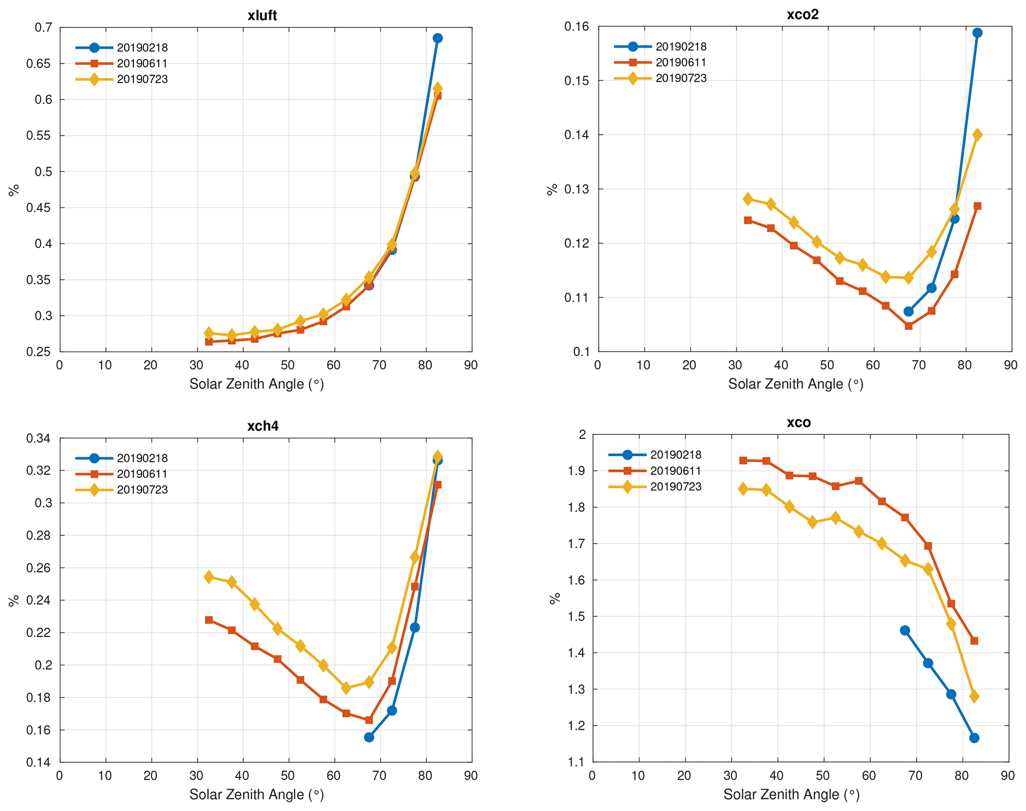
Figure 26These figures show the sum in quadrature of all the errors plotted in Fig. 23 for all three dates. The errors plotted here are for Xluft, , , and XCO.
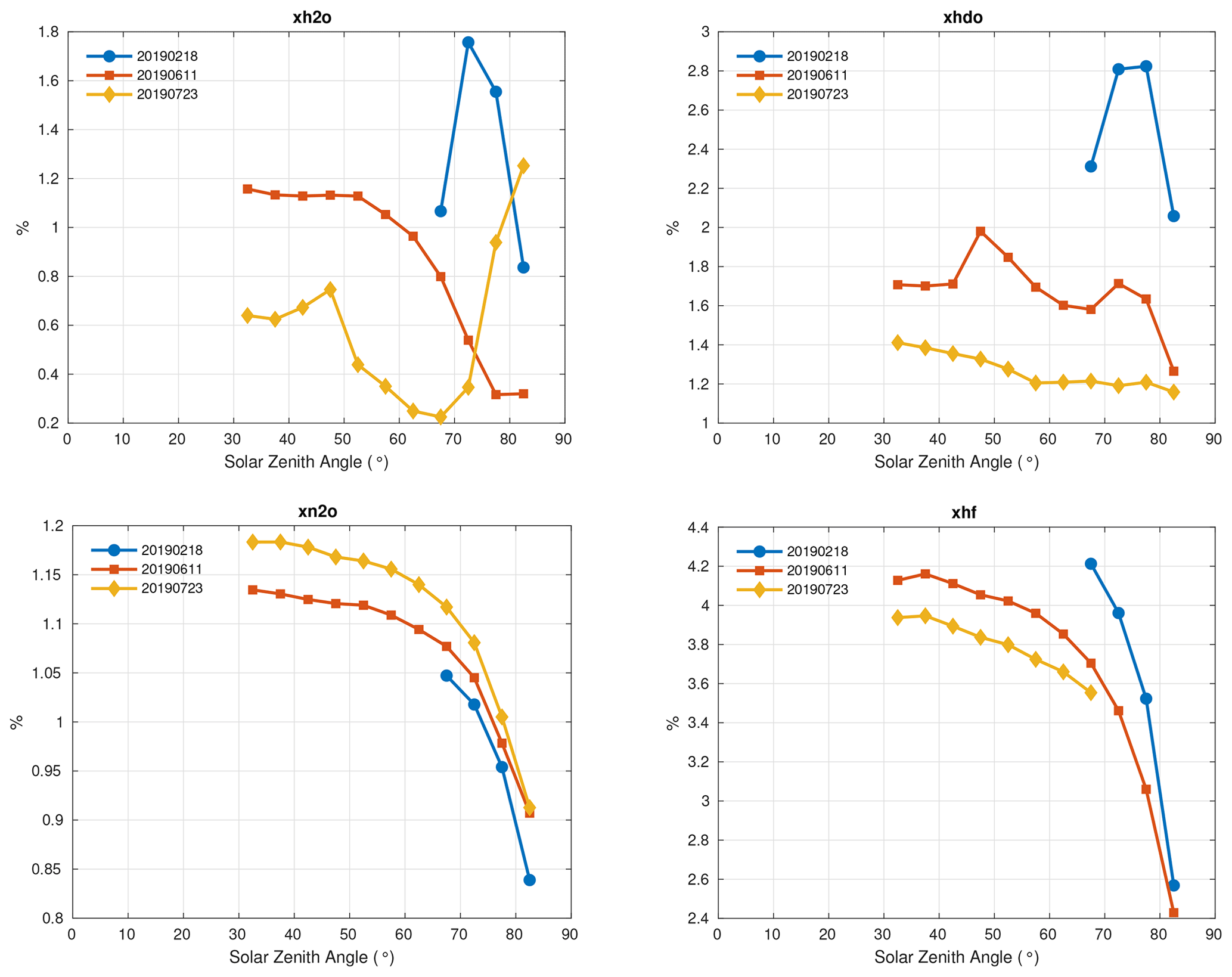
Figure 27As in Fig. 26 but for , XHDO, , and XHF. XHF values above 68° SZA are not available on 23 July 2019 because the HF lines were blacked out by H2O absorbance.

9.19 Uncertainty estimate comparison
For six products (, , , , XCO, and ) we can compare the uncertainty estimates derived from the error budgets with those computed from in situ comparisons similar to those in Sect. 8.3 but with one difference: the comparisons in Sect. 8.3 use the in situ vertical profiles as the prior trace gas profiles in the TCCON retrievals; the in situ comparisons in this section use standard TCCON GGG2020 prior profiles. For the in situ uncertainty, we use the mean absolute deviation (MAD) of the TCCON Xgas values from the in situ Xgas values after removing the mean bias for each Xgas (i.e., the correction factor in Table 4). We use MAD over standard deviation because it is less sensitive to outliers. To convert the percent error from the error budget into a column-average dry mole fraction, we use the mean total percent error across all 3 stated days used in the error budget (18 February, 11 June, and 23 July 2019) binned by SZA in 5° increments. We interpolate this to the mean SZA of all spectra used in the in situ comparison for that gas and multiply this interpolated mean percentage by the mean TCCON Xgas value across all the in situ comparisons. We then add the error from the in situ data to the error budget value in quadrature for comparison to the MAD. The results are presented in Table 5.
Table 5A comparison of typical errors calculated from the differences between TCCON and in situ Xgas values (“MAD” in the table, i.e., mean absolute deviation), errors calculated from the error budget (“Budget” in the table), and the quadrature difference of the error budget and in situ error (“MAD – in situ”). “Gas” indicates which Xgas product the error is for and the units of the values in the last four columns. “SZA” gives the solar zenith angle for which the error budget percent was taken to calculate the “Error budget” column. ϵin situ gives the total 2σ uncertainty of the in situ data. The first number in this column is the result of formally propagating the in situ error into its MAD value, and the second number in parentheses is the simple mean across all the TCCON in situ comparisons. Note that ϵin situ includes estimated uncertainty due to unmeasured parts of the profile; see Table C7 in the Appendix for a breakdown of the individual error components.
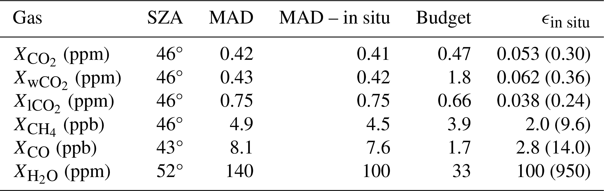
It is important to acknowledge that the MAD values calculated from the in situ comparison are (for most gases) potentially less than the error budget for several reasons. First, in situ profiles are usually taken when the target TCCON station is near optimal performance; thus, those comparisons are unlikely to capture the full range of error sources. Second, the in situ profiles are heavily concentrated over certain TCCON sites, also limiting how representative they are. Finally, the TCCON Xgas values compared against the in situ values are averaged over a minimum of 2 h. This will reduce sources of random error. However, we believe this is still a worthwhile evaluation of measurement accuracy because (a) there is real physical variation in the atmosphere during the in situ profile, and the time averaging is necessary to account for that, and (b) many of the factors considered in the error budget will not average out over the coincidence window. For example, angular or shear misalignment of the instrument would be essentially constant over an entire day.
For three Xgas products (, , and ) the MAD and error budget estimates are similar, which gives us confidence in the error budget estimates. For , the error budget estimate is much larger than the MAD value. It may be that the error budget tested larger errors in the stratosphere temperature or VMR prior profile than those that were observed during the in situ comparisons as the product is more sensitive to the upper atmosphere than the other CO2 products in GGG2020. Pressure errors could be another source of the overestimation, but the pressure perturbation test was designed to avoid introducing an overly large perturbation to the stratosphere. As we treat the in situ-derived errors as a lower estimate, this situation is acceptable but will be investigated in the future.
Both XCO and had larger MAD values than their respective error budgets. For XCO, the difference in error estimates is 5.9 ppb. The “MAD – in situ” column uses the propagated value for ϵin situ (2.8 ppb). The uncertainty in individual comparisons (the parenthetical numbers in Table 5) is quite a bit larger; if part of this error is systematic (such as from drift in calibration tanks, e.g., Andrews, 2019), that could explain the remaining difference. For , this is because of uncertainty in the radiosondes used to be compared against. The radiosondes used at ARM have a 4 % or 5 % uncertainty in relative humidity (https://www.arm.gov/publications/tech_reports/handbooks/sonde_handbook.pdf, last access: 10 April 2023). When we propagate this uncertainty to the mean absolute deviation, it works out to 100 ppm. Subtracting this in quadrature from the MAD estimate reduces the mismatch in error estimates, but ∼70 ppm remains. We do note that, in Fig. 16f, the TCCON and radiosonde values for Xluft≈1 (i.e., when the TCCON instrument was operating best) seem to be systematically >1 at Darwin and <1 at Lamont, suggesting that subtracting the in situ bias in quadrature might be underestimating its impact on the TCCON–radiosonde mismatch.
Table 6Known biases in GGG2020 data along with current action taken by the TCCON data providers or recommended for users to take to mitigate the impact of each bias. The final column identifies future plans to correct each bias, with the GGG version in which those corrections will be implemented.

All TCCON GGG2020 data are linked through https://tccondata.org (last access: 22 April 2024) and stored as DOI-tagged data sets on CaltechDATA (https://data.caltech.edu, last access: 22 April 2024). Each TCCON site has a separate repository and DOI on CaltechDATA; these are listed in Table 2. If a future correction requires a revision of previously published data, that revision will receive a new DOI. Users are encouraged to check https://tccondata.org for the latest revisions of data rather than relying on Table 2. A repository containing the full set of TCCON GGG2020 data is also available on CaltechDATA with the DOI https://doi.org/10.14291/TCCON.GGG2020 (Total Carbon Column Observing Network (TCCON) Team, 2022). Users are asked to cite the individual sites' data records rather than the combined record as this helps track usage of site data and thus support the ongoing operation of these sites. We provide a citation generator at https://tccondata.org/metadata/siteinfo/genbib/ (last access: 22 April 2024). All data are provided in netCDF format, and additional documentation for the data is available at https://tccon-wiki.caltech.edu/ The TCCON community, 2024. The GGG2020 retrieval software is archived on CaltechDATA (https://doi.org/10.14291/tccon.ggg2020.stable.R0, Toon, 2023), as well as being publicly available through GitHub at https://github.com/TCCON/GGG (last access: 11 July 2023).
The GGG2020 TCCON data product incorporates numerous improvements to the GGG retrieval, based both on first-principle understanding and empirical evaluation. To review, we note the following:
-
The interferogram-to-spectrum conversion has added checks and diagnostics for detector nonlinearity or saturation, as well as a modification to the phase correction that reduces bias between forward and reverse scans of the interferometer.
-
The solar and telluric spectroscopic line lists used in the GGG forward model have been updated to reflect new laboratory and atmospheric and solar observing studies, to include non-Voigt line shapes and line mixing, and to reduce an observed temperature and water dependence in the O2 column amounts.
-
The a priori inputs of atmospheric state (temperature, pressure, and composition) have increased temporal resolution, and the trace gas profiles have been updated to better reflect both atmospheric growth rates of key species and gradients in their mixing ratios across the tropopause.
-
Improvements have been made to fitting the continuum and channel fringes in the spectra.
-
A more flexible air mass correction was applied to the Xgas value from individual spectral windows rather than multi-window averages of said values.
-
We made a change to how retrieved Xgas values from multiple spectral windows measuring the same gas are averaged together that eliminates the dependence on how many observations were averaged at once.
-
We applied an updated in situ correction factor that increases the number of profiles used to tie TCCON to the calibration scales used by in situ GHG measurements.
-
We made improvements in terms of user friendliness in how AKs and prior profiles are reported in public files.
There remains work to be done to further improve the TCCON data product. Implementing the capability in GGG to account for errors in ILS remains a high priority. This was planned for inclusion in GGG2020 but could not be completed in time. It is expected that this capability will be an important tool to eliminate the bias seen in comparison with in situ profiles as Xluft deviates from its nominal 0.999 value. A second high-priority objective is to investigate the temperature dependence seen in the N2O and (to a much lesser extent) CH4 data and to correct the underlying spectroscopic terms.
We currently plan to develop minor releases, GGG2020.1 and GGG2020.2, within the next several years to address the highest-priority issues (Table 6) that will include additional post-processing bias corrections to address the bias of versus Xluft and and versus temperature. This may allow us to release data from the early years of several sites, currently flagged as poor quality due to out-of-bounds Xluft, as well as to improve the data substantially. As this would be a post-processing-only update, the reprocessing could be completed very rapidly.
At time of writing, 26 TCCON sites have reprocessed their existing data with GGG2020. Several sites are still in the process of carrying out this reprocessing, in many cases to improve the data quality based on new diagnostics available in GGG2020. Work is ongoing toward completing these sites' reprocessing. Extensions to the existing data records will be released monthly going forward.
Abbreviations used in this paper are listed in Table A1. The retrieval windows used in GGG2020 are given in Tables A2 and A3.
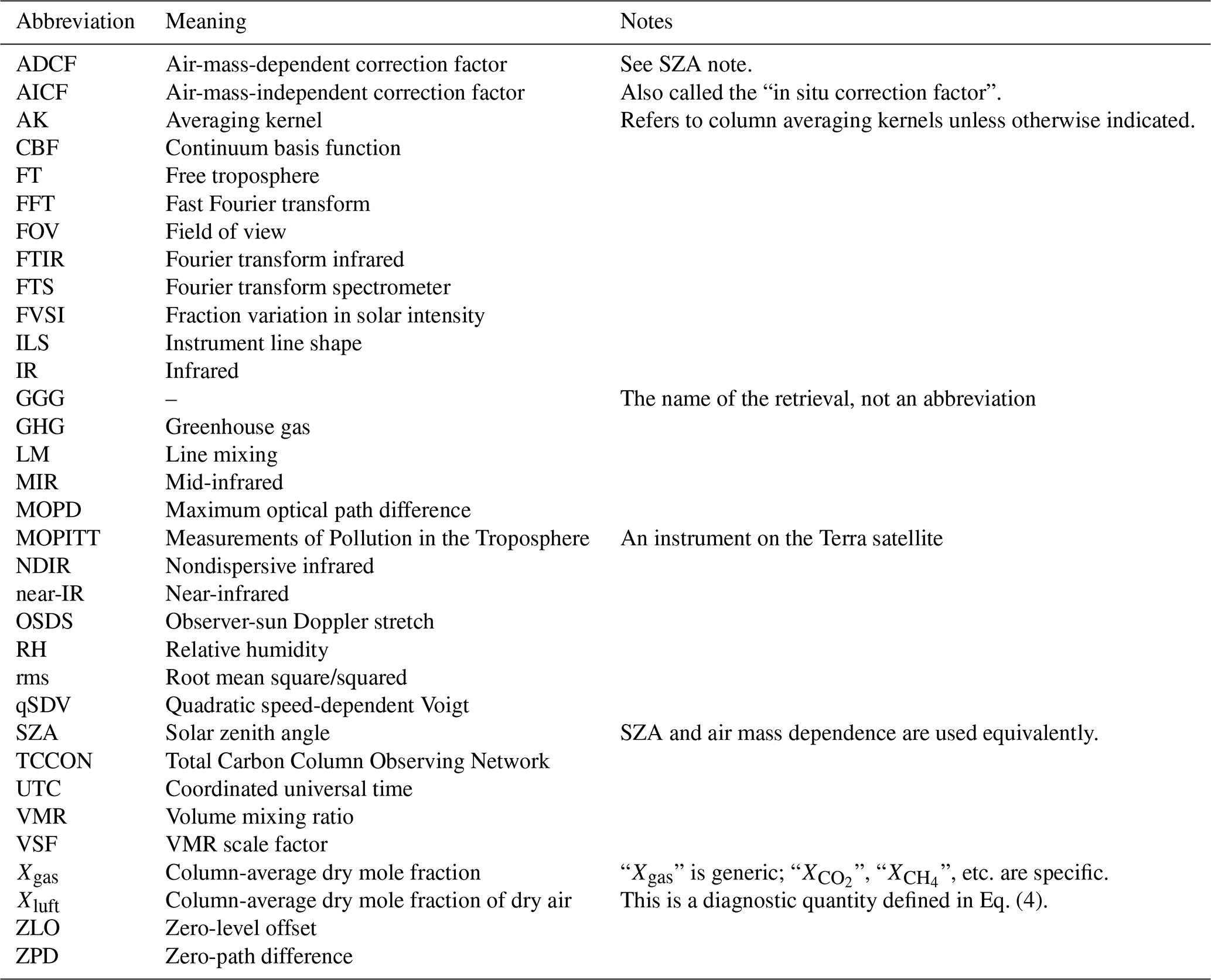
Table A2Retrieval windows used for CO, N2O, CH4, O2, and the three CO2 products in GGG2020. “Freq. range” gives the edges of the window. “Target gas” gives the gas whose column abundance is obtained from that window. “Other gases” lists gases that are retrieved as interferents in that window (note that the lCO2 window includes several CO2 isotopologs, and the O2 window includes the O2 collision-induced absorption). “qSDV” and “LM” indicate which species in that window include non-Voigt speed-dependent and line-mixing line shape information, respectively, for their main lines (Sect. 6.2). A dash in these columns indicates no gas has speed dependence or line-mixing information, respectively. Note that CH4 uses full line mixing, while CO2 uses the Rosenkranz approximation. “No. CBF” indicates the number of basis functions used to fit the continuum in that window (Sect. 7).
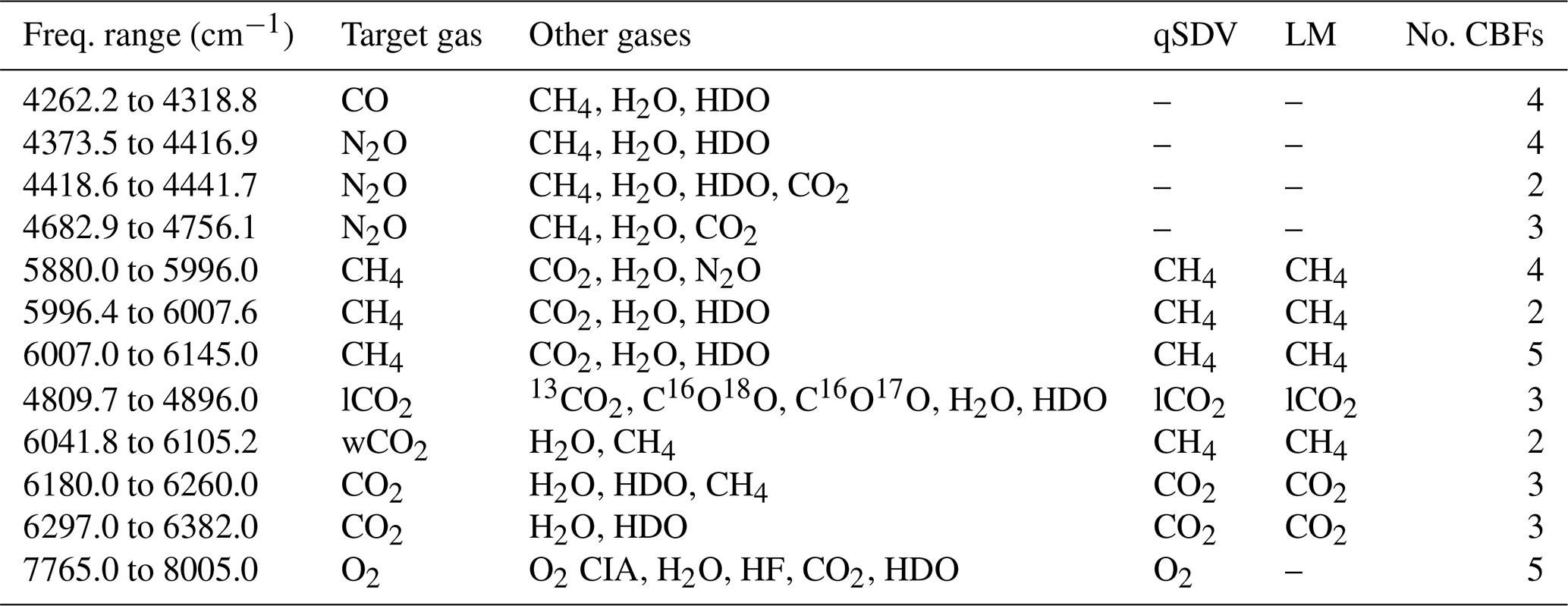
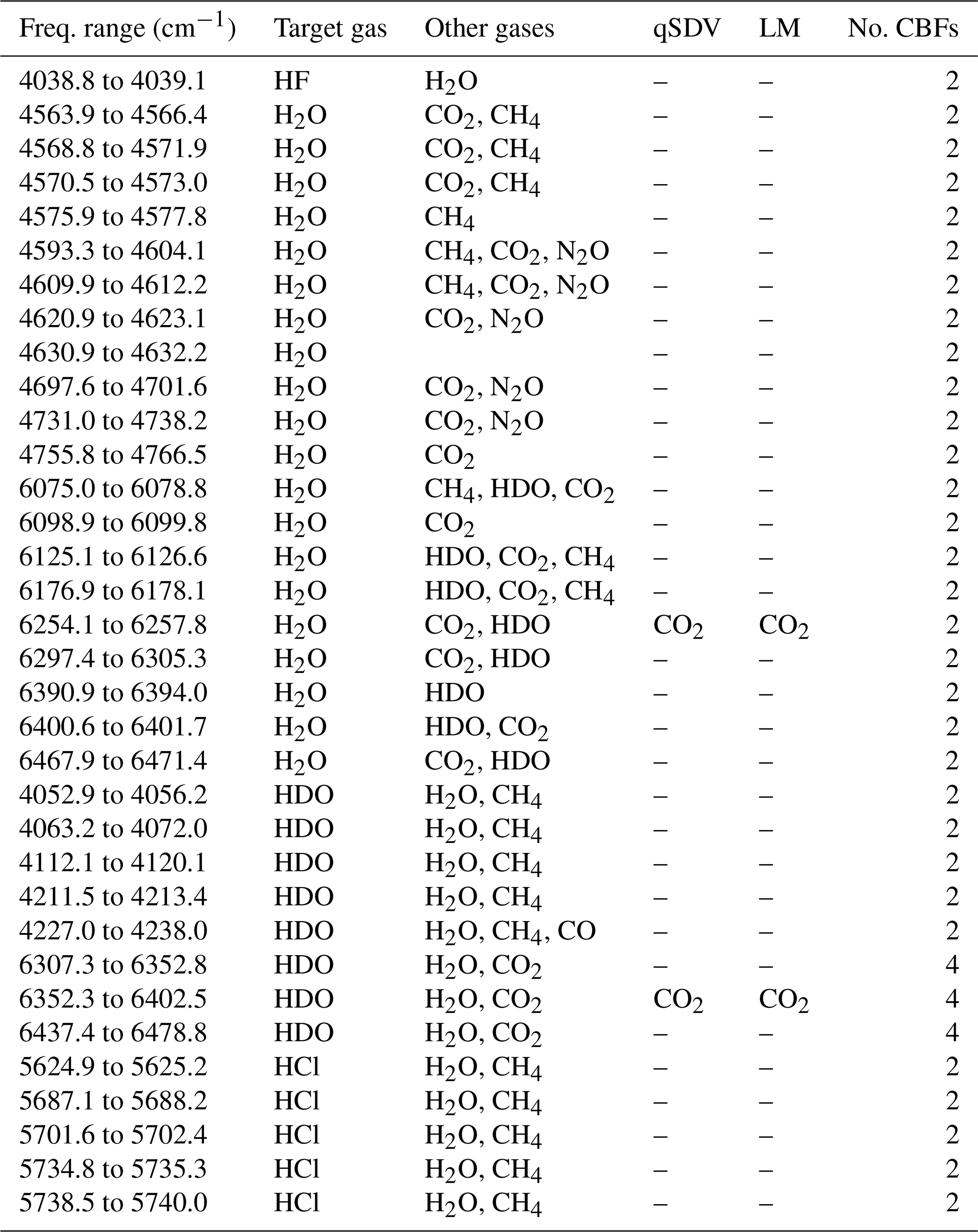
For completeness, we include the error budget figures equivalent to Figs. 23–25 for February and July at East Trout Lake in Figs. B1 to B6. February is extremely cold (−30 to −15°C) and dry (< 500 ppm ), with short days and large solar zenith angles. July is warm (20 to 30 °C) and humid (3000 to 4500 ppm ), causing the HF absorption feature to be blacked out by adjacent H2O lines at higher solar zenith angles, causing unreliable retrievals of HF.

Figure B1The 18 February 2019 error budget from East Trout Lake. The figures show the percent difference between the perturbed test and the standard retrieval plotted as a function of solar zenith angle. The retrievals plotted here are Xluft, , , and XCO.
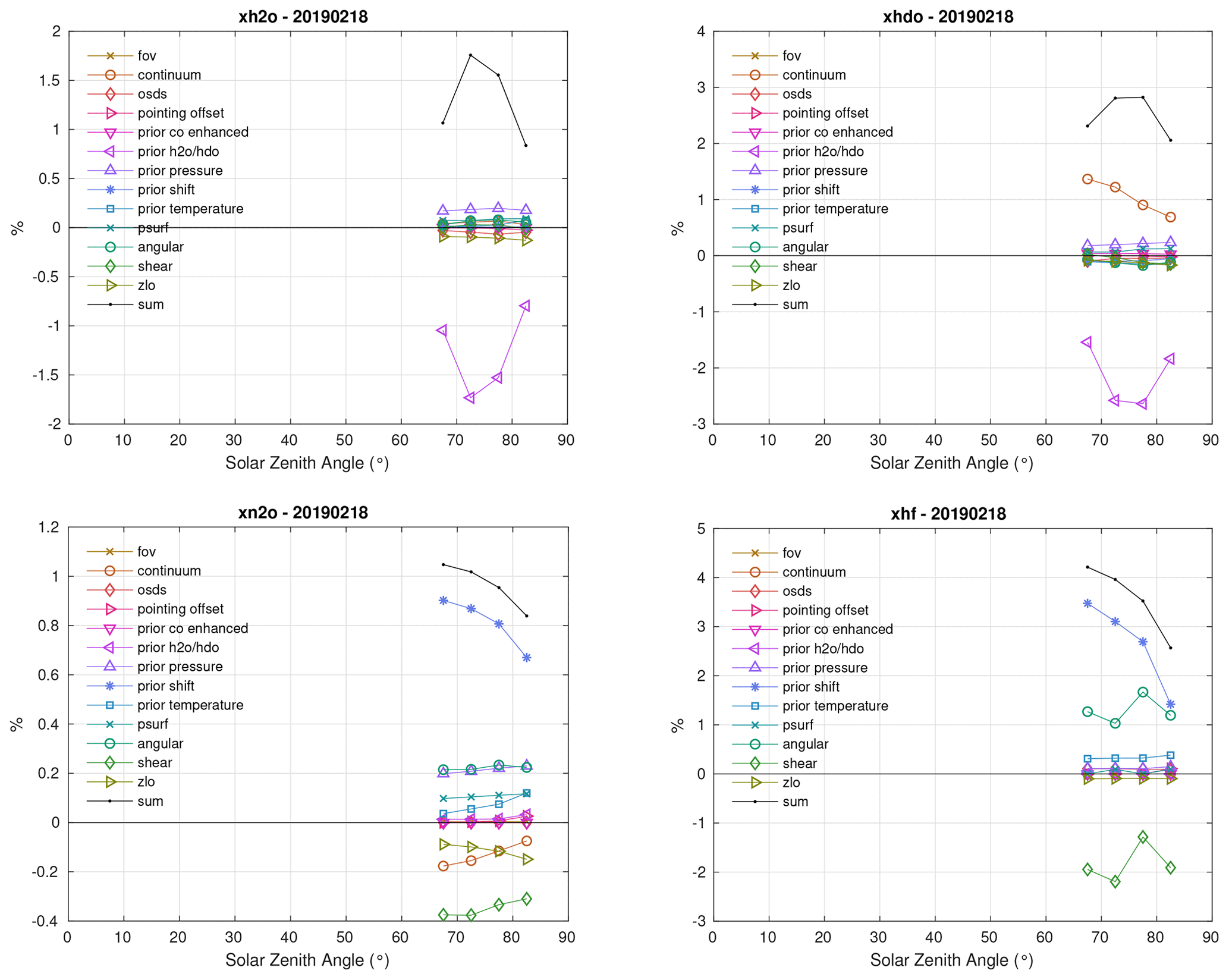
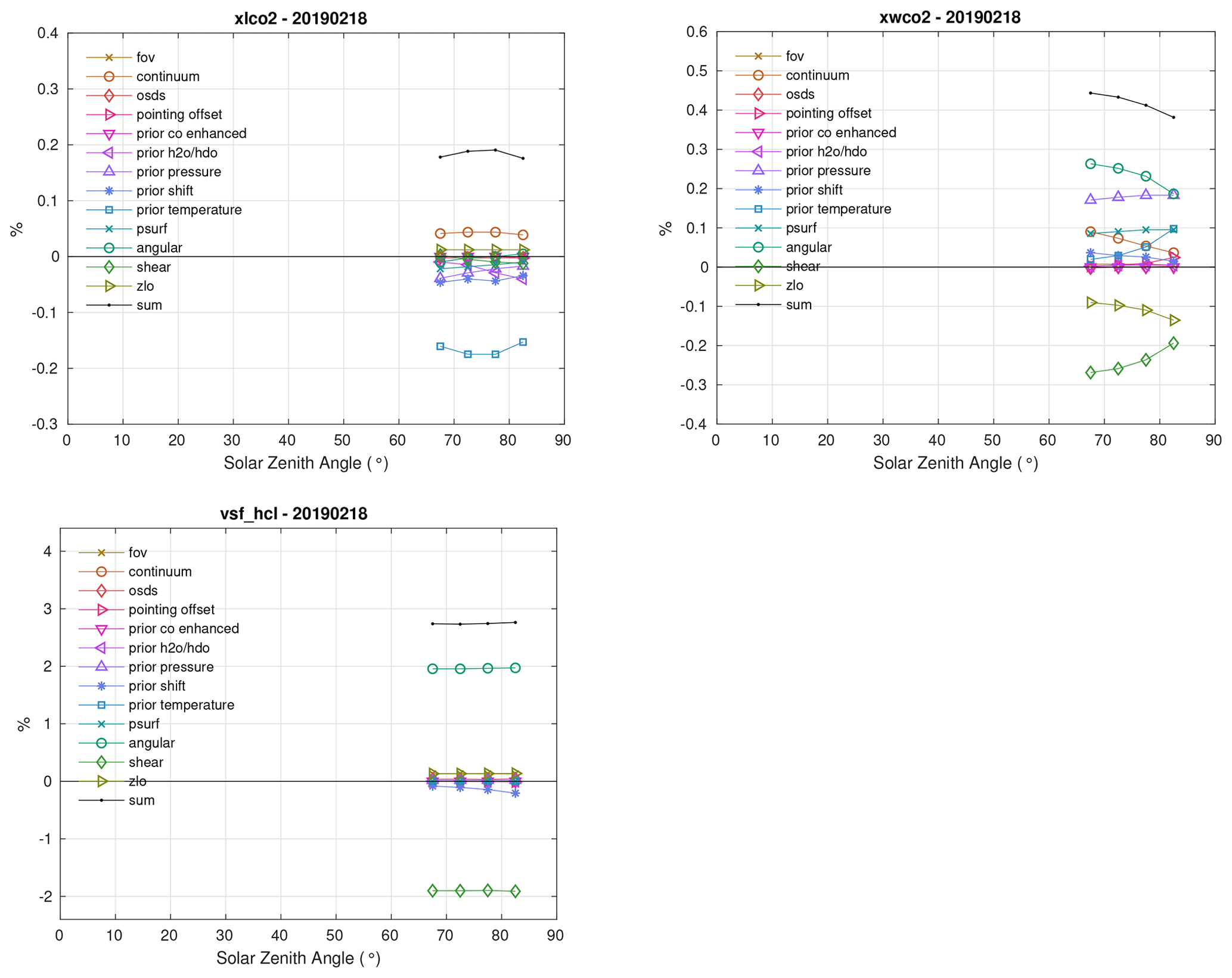

Figure B4The 23 July 2019 error budget from East Trout Lake. The figures show the percent difference between the perturbed test and the standard retrieval plotted as a function of solar zenith angle. The retrievals plotted here are Xluft, , , and XCO.
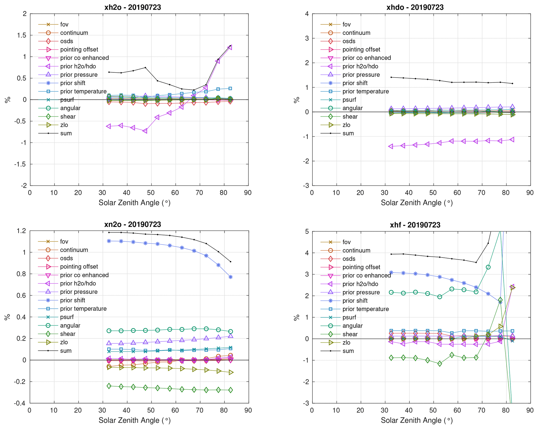

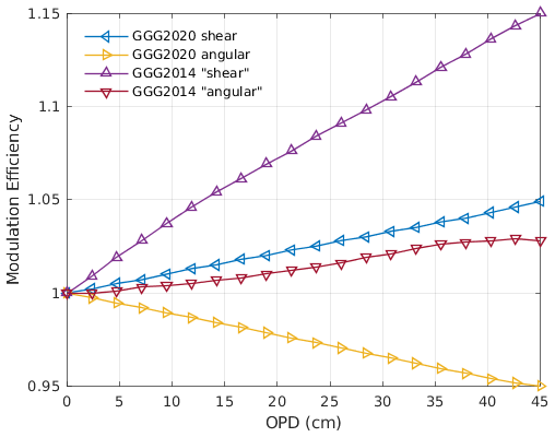
B1 ILS
We created synthetic spectra in GGG2020 with different ILS errors following the formulation for the “shear” and “angular” misalignments tested for the GGG2014 error budget and for the new formulation in GGG2020. We then passed these synthetic spectra through an ILS quantification program called LINEFIT (v14.8) (Hase et al., 1999), which calculates the modulation efficiency and phase error of the spectra. Here, we plot the LINEFIT-derived modulation efficiencies for these four cases in Fig. B7. The GGG2020 shear and angular misalignments represent a ramp-up and ramp-down from 1.0 at zero path difference to 5 % offsets at 45 cm optical path difference, as expected. Unfortunately, the GGG2014 “shear” and “angular” misalignments both model shear misalignments of different magnitudes. The GGG2014 “shear” case is, in fact, more like a 15 % ramp up as a function of optical path difference, and the GGG2014 “angular” case is more like a 3 % ramp up. This will essentially double the inferred error from the ILS in GGG2014 when compared with GGG2020.
C1 CO2, CH4, CO
In situ profiles for CO2, CH4, and CO were drawn primarily from the NOAA CO2 ObsPack (Cooperative Global Atmospheric Data Integration Project, 2019), the NOAA CH4 ObsPack (Cooperative Global Atmospheric Data Integration Project, 2020), the NOAA AirCore data set (Baier et al., 2021), additional AirCore launches at the Sodanklyä and Nicosia TCCON sites, the Infrastructure for Measurement of the European Carbon Cycle (IMECC) campaign, and the GO-AMAZON campaign. The ObsPack contains data from numerous providers across different institutions; Tables C1 and C2 provide a detailed breakdown. For the NOAA ObsPack Aircraft and AirCore profiles, the procedure used to match these data to TCCON sites will be detailed in the following subsections. For the remaining sources, the profiles were already associated with specific TCCON sites; thus, no colocation was required.
All airborne data sources used for these profiles are listed in Tables C1 and C2. Ground data used to extend some of the profiles to the surface are listed in Table C3.
Table C1Airborne profile data used in the AICF calculation. “CO2 ObsPack” is the CO2 GLOBALVIEWplus v5.0 ObsPack (Cooperative Global Atmospheric Data Integration Project, 2019), and “CH4 ObsPack” is the CH4 GLOBALVIEWplus v2.0 ObsPack (Cooperative Global Atmospheric Data Integration Project, 2020). The “TCCON sites” column indicates at which sites data were used; the IDs are mapped to locations in Table 2, and the numbers of profiles per site are given in Tables C4 and C5. In the “Providers” column, affiliations are given in parentheses. If only one affiliation is listed, it applies to all individuals named. Abbreviations: NASA for National Aeronautics and Space Administration, LaRC for Langley Research Center, Harvard U. for Harvard University, CSUSB for California State University San Bernadino, GSFC for Goddard Space Flight Center, NCAR for National Center for Atmospheric Research, NOAA for National Oceanic and Atmospheric Administration, GML for Global Monitoring Laboratory, FMI for Finnish Meteorological Institute, CARE-C for Climate and Atmosphere Research Center, LSCE/IPSL for Laboratoire des Sciences du Climat et de l'Environnement.
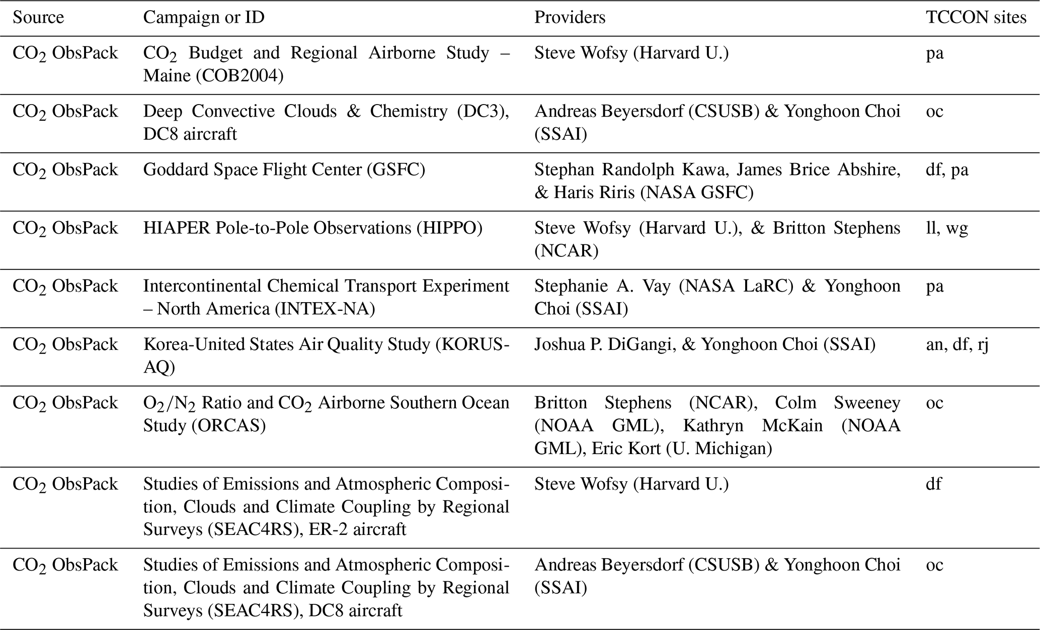
Table C2Table C1 continued. Abbreviations: ARM for Atmospheric Radiation Monitoring facility. n/a – not applicable

Table C3Ground in situ data used in validating the priors. “CO2 ObsPack” is the CO2 GLOBALVIEWplus v5.0 ObsPack (Cooperative Global Atmospheric Data Integration Project, 2019), and “CH4 ObsPack” is the CH4 GLOBALVIEWplus v2.0 ObsPack (Cooperative Global Atmospheric Data Integration Project, 2020). The “TCCON sites” column indicates which sites profiles were used at, and the IDs are mapped to locations in Table 2. In the “Providers” column, affiliations are given in parentheses. If only one affiliation is listed, it applies to all individuals named. Abbreviations: NDIR for nondispersive infrared, NOAA GML for National Oceanic and Atmospheric Administration Global Monitoring Laboratory, PSU for Pennsylvania State University, U. of WI for University of Wisconsin, USGS for United States Geological Survey, LBNL for Lawrence Berkeley National Laboratory, ARM for Atmospheric Radiation Measurement, CRDS for cavity ring-down spectroscopy, NIWA for National Institute of Water & Atmospheric Research Ltd.

Table C4The number of profiles in the CO2 in situ correction from each campaign or other data source identified and used for each TCCON site. The “Found” column gives the number of profiles identified for that campaign and site, and the “Used” column gives the number of those profiles which could be used in the in situ comparison after matching with TCCON data. The definitions of the site IDs can be found in Table 2; “we” refers to an instrument in Jena, Germany, for which GGG2020 data were not available at time of writing.

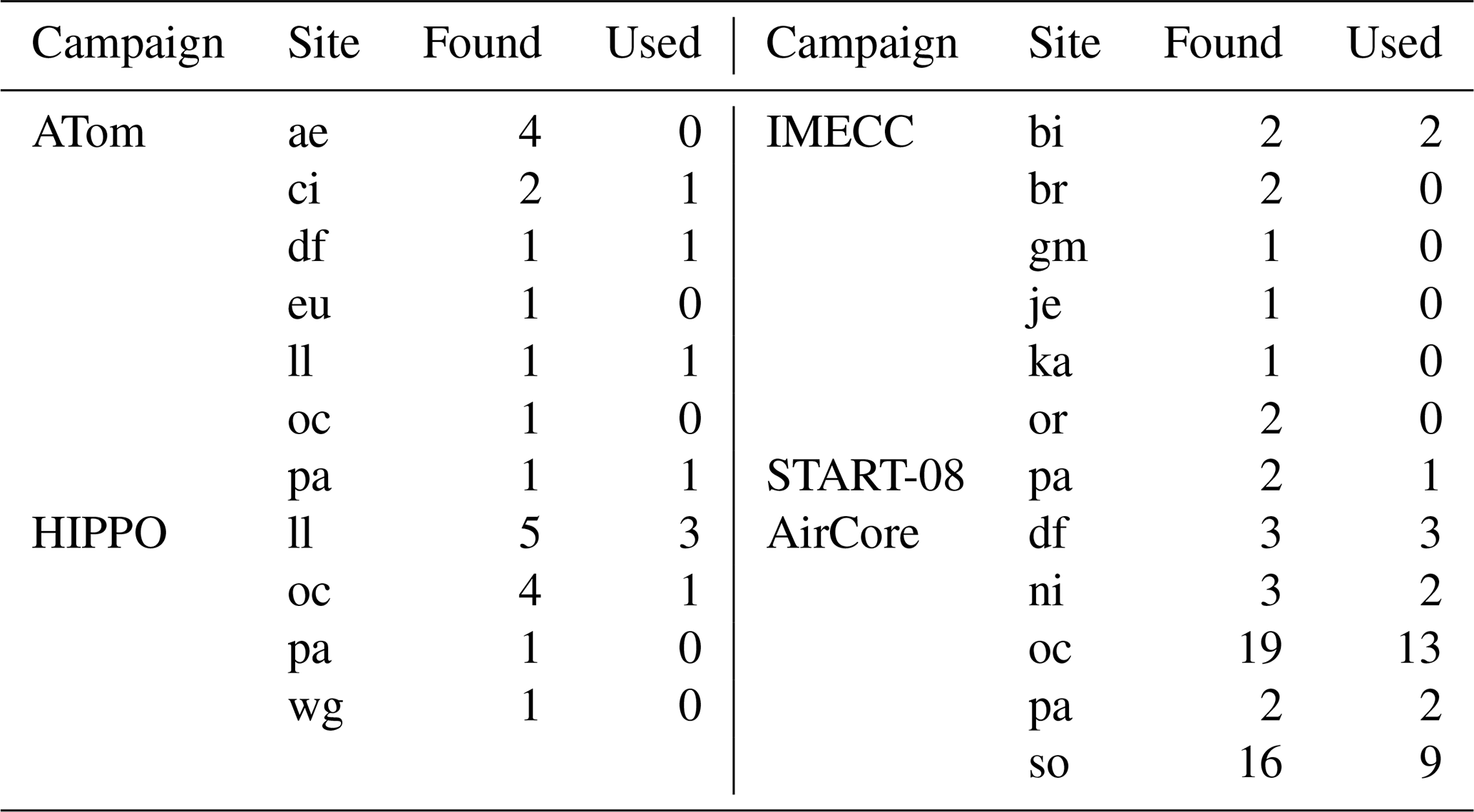
C1.1 ObsPack
The ObsPack data are provided as a single time series per measurement campaign or similar source. To extract individual profiles from these files, we performed the following:
-
We scanned all files for data points within 2° (total distance) of an active TCCON site. When one was found, we stored the list of data points surrounding it in time within a box of 10° longitude and 5° latitude, centered on the TCCON site as a “chunk”. A chunk extends forward and backward in time from the point closest to the TCCON site and stops at the first data point in each direction that is outside the 10°×5° box. Any profiles derived from this chunk were assigned to the TCCON station it passed closest to.
-
We further filtered the chunks based on the lowest altitude, highest altitude, number of data points, and minimum distance to a TCCON site. This step was done interactively to find the filtering criteria that gave the best balance between the number of chunks retained and the usefulness of the profile(s) within the chunk. The final criteria used were
-
minimum altitude below 2000 m
-
maximum altitude above 7500 m
-
at least 20 data points
-
approached within 0.1° of a TCCON station.
-
-
These filtered chunks were then individually evaluated, and specific data points within them were chosen by hand to be used as profiles. In this process, we considered the latitude–longitude position of the aircraft, the profile of altitude versus time, and the profile of CO2 or CH4 versus altitude. We generally selected as profiles times when the aircraft was consistently ascending or descending and excluded times of level flight. However, this had to be handled on a case-by-case basis to allow for profiles with a period of level flight in between two legs of an ascent or descent. If a chunk contained multiple ascending or descending legs, we would split them if
-
there was a clear separation in time, or
-
the legs measured different air masses (evidenced by different CO2 or CH4 dry mole fractions).
-
-
For each profile, we checked for ground data in the ObsPack that can be used to extend the profile to the surface. We identified which ground files in the ObsPack were near which TCCON sites by hand. We interpolated any data within 4 h of the lowest-altitude measurement in a profile to the time of the lowest-altitude profile measurement. In cases where ground data were only available before or after the lowest profile measurement, we used the closest ground data in time.
C1.2 AirCore
As AirCore data intrinsically provide discrete profiles, matching these data to TCCON sites was much simpler. For NOAA AirCores, we search all files for those where the mean latitude and longitude of the profile were within 1° (total distance) of a TCCON site. We use a looser distance compared to the aircraft as it is unlikely that an AirCore would be within 1° of a TCCON site by happenstance if it was not intended to match with that TCCON. However, since it is possible that the balloon trajectory drifted significantly, depending on the winds, we use the looser distance criterion to allow for that.
C2 H2O
Profiles for the H2O AICF come from radiosonde data provided by the Department of Energy Atmospheric Radiation Measurement (ARM) facility (Keeler et al., 2001). The data were downloaded from https://adc.arm.gov/discovery/#/results/instrument_class_code::sonde%2Fprimary_meas_type_code::atmtemp (last access: 11 July 2023) in March 2021. Two ARM sites are close enough to TCCON locations to be useful: the Southern Great Plains (SGP) site's Central Facility (facility code C1) is near the Lamont, OK, USA, TCCON site, and the Tropical Western Pacific (TWP) site's Darwin facility (code C3) is near the Darwin, Australia, TCCON site.
These facilities produce more radiosonde observations than we can feasibly use in the AICF calculation; thus, we must choose a subset. We use the following steps for each site:
-
Identify radiosonde profiles that are coincident with another trace gas profile (CO2, CO, CH4, or N2O).
-
Identify radiosonde profiles not in the set identified in step 1 that have at least 30 TCCON spectra within ±3 h of the time of the profile's lowest-altitude measurement.
-
Combine the profiles from step 1 with randomly selected profiles from step 2 to collect 50 total profiles. We use a seed of 42 – chosen in reference to The Hitchhiker's Guide to the Galaxy – to ensure repeatability across runs.
-
Finally, remove any profiles from this set of 50 that have a maximum altitude <15 km.
Once we have assembled a pool of radiosonde profiles, we convert the relative humidity (RH) values stored in the files to water dry mole fractions. Based on the convention described in Miloshevich et al. (2006), we assume that the definition of RH is the ratio of water vapor pressure to the saturation water vapor pressure over liquid water and calculate the H2O dry mole fraction as
where RH is the relative humidity as a fraction (i.e., 0 to 1), SVP is the saturation vapor pressure of water over liquid water calculated using Eq. (6) of Miloshevich et al. (2004) (see also Eq. 15 of Wexler, 1976), and p is the atmospheric pressure (in the same units as SVP).
C3 Constructing full profiles
In order to ensure a proper comparison between the in situ and TCCON column amounts, the in situ profiles must extend to the top of the TCCON retrieval altitude grid at 70 km. No aircraft- or balloon-borne profile reaches this altitude; therefore, similarly to Wunch et al. (2010), we extend the in situ profiles using the GGG2020 prior profiles (Laughner et al., 2023).
The differences between Wunch et al. (2010) and our approach stem from the fact that (1) the GGG2020 priors do a better job of representing trace gas profiles in the stratosphere, and (2) we have enough additional profiles over TCCON sites to be selective about which ones we use. This is why we filtered the ObsPack data to chunks that have data up to at least 7500 m altitude (Sect. C1.1) to limit the altitude that needs to be filled in above the top of the profile.
There are three ways that profiles are extended up to 70 km altitude, depending on their top altitude:
-
If the profile's top is above 380 K potential temperature (i.e., reaches the stratospheric overworld) then we append the GGG2020 priors for levels above the profile top.
-
If the profile's top is below 380 K potential temperature but at or above 7.5 km then the in situ profile's values are binned to the same altitude grid (see below), and then we do a constant-value extrapolation of the top binned value up to the tropopause altitude. We use the GGG2020 prior above 380 K potential temperature again and connect the two parts of the profile by linearly interpolating the trace gas dry mole fractions with respect to potential temperature between the tropopause and 380 K. This case covers profiles where the top of the measured profile is expected to be a better representation of the unmeasured free troposphere than the GGG2020 priors.
-
If the profile's top is below 7.5 km, then we use the GGG2020 priors for all levels above the profile top. The case assumes that profiles that do not reach above 7.5 km do not constrain the free troposphere well enough to supplant the GGG2020 priors. While we filtered the ObsPack data for chunks that have data above 7.5 km, we still have a few profiles with ceilings below 7.5 km from chunks that needed to be split into multiple profiles.
For no. 2, we calculate the binned in situ profile values for the highest altitude of the GGG retrieval grid below the in situ profile's ceiling (zGGG,k) as follows:
Figure C1 shows an example of the weights for one short profile at the Armstrong TCCON site.

Figure C1An example of the weighting functions from Eq. (C4). Lines indicate the weights applied to the observed mole fractions, and circles indicate the GGG altitude grid levels that correspond to those weights – like colors match.
There is a special case for CH4 applied when integrating the in situ profile to calculate the in situ-derived . Previous work (e.g., Washenfelder et al., 2003; Saad et al., 2014, 2016) established that there is a strong correlation between CH4 and HF in the stratosphere. Since this correlation is encoded into the GGG2020 priors (Laughner et al., 2023), we can use the difference between the prior and posterior HF column (which is almost entirely found in the stratosphere) from the TCCON retrievals to adjust the levels in the in situ CH4 profiles that use the GGG2020 profiles.
Specifically, when calculating the in situ , we get the slope of CH4 vs. HF mixing ratios used by the GGG2020 priors for the year and region (tropics, midlatitudes, or polar vortex) of the profile (see Sect. 3.5 and Fig. 11 of Laughner et al., 2023). We then multiply this slope by the difference between the prior and median posterior HF profile of all the TCCON observations matched with the in situ profile in question in order to get the expected change in the CH4 priors to better match the true stratospheric profile. Finally, we multiply this profile difference by the TCCON AK and integrate only the levels in the total in situ profile obtained from the GGG2020 priors. The integration uses Eq. (10) and adds the integrated change to the in situ as a posterior adjustment.
Again, note that this correction is only applied when integrating the in situ profiles to obtain the true value to compare the TCCON retrievals against. When using the in situ profiles as priors in the TCCON retrievals, the levels taken from the GGG2020 priors are not adjusted in this fashion.
C4 Grouping temporally proximate profiles
There are several cases where multiple profiles are available within a short time of each other (such as different legs of a missed approach or duplicate AirCore launches). Because we use the observed profiles as the prior in the TCCON retrievals from which the AICF is derived, this presents a technical challenge. Ideally, we want to use the same prior for all retrievals matched up with a given profile for comparison. Our temporal coincidence criterion can be up to ±3 h; therefore, in cases with two or more profiles within a few hours, if we used for each TCCON retrieval the observed priors closest in time to it, this would result in a change in the prior partway through our coincidence window.
Our solution was to merge profiles close enough in time for this to occur but only for use as priors. Each individual observed profile still contributes one point in Fig. 16. This does mean that the prior will not exactly match any of the observed profiles those retrievals are compared against, but we consider that to be an acceptable error, given that we do apply an AK correction to the integrated in situ profile.
To find profiles that need to be merged, we first identify which TCCON observations would match with that profile. We ignore the quality filtering criteria from Sect. 8.3.1 during this step and only try to find the time window (±1, 2, or 3 h) necessary to match at least 30 TCCON observations to each profile. If any two profiles from the same TCCON site are matched to any of the same TCCON observations, they are grouped together in the list of profiles to be averaged together when creating the custom priors in Sect. C5. This initial list is written out to a text file so that it can be modified by hand later, as needed.
C5 Running custom TCCON retrievals
As mentioned in Sect. 8.3, when we run the TCCON retrievals for the AICF calculation, we use as custom priors the in situ profiles that a given TCCON observation will be compared against. This reduces error in the TCCON Xgas value that arises from an incorrect prior profile and thus improves the accuracy of the AICF. There are several technical considerations in how we handle this matching. In order to make those considerations clear, let us first describe how the GGG retrieval accepts inputs describing both the prior profiles and the TCCON observations to retrieve on.
GGG takes a list of TCCON spectra to retrieve as input in the “runlog” file. This lists each spectrum on which to run the retrieval in order. For the AICF retrievals, we combined all the spectra from all the relevant TCCON sites into a single runlog.
The priors (including temperature and pressure, as well as trace gas mixing ratios) are written to a “.mav” file. This file is organized into blocks. Each block indicates the first spectrum from the runlog which the priors contained in the .mav block apply to. During the retrieval, GGG iterates through the spectra contained in the runlog. When it reaches the spectrum defined as the first spectrum of the next block in the .mav file, it loads the priors from that block before continuing.
In inserting the in situ profiles into the .mav file as priors, we had three objectives:
-
retain the standard priors for gases and times for which we did not have in situ profiles available
-
ensure that the in situ profiles were used as priors for any spectra that they might be compared against
-
ensure that any in situ profiles were only applied to the TCCON site where and on the day that they were measured.
To meet these objectives, our approach to inserting the in situ profiles as priors was as follows:
-
Divide the runlog into chunks by site and day so that each chunk only has spectra from one site on one day.
-
For each unique site–day chunk, collect all the in situ profiles from that day.
-
Average together any in situ profiles grouped together in the list created in Sect. C4. For this, we used an approach that considers whether each in situ profile contributed observations to a given level in the regridded profile. For a level on the retrieval grid where none of the in situ profiles provided any data points (i.e., the observed profiles were extrapolated or had the GGG2020 prior appended to it), both profiles are weighted equally. For a level where at least one of the in situ profiles had observed data, each profile is weighted by the fraction of data for that level that came from observations.
-
For gases that only have one profile (after averaging) for that site or day, assign that profile to all the .mav blocks for that site or day.
-
For gases that have multiple profiles that are not merged together (Sect. C4), use the first profile in the day for all .mav blocks up until the first spectrum that could be compared with the second profile in the day (for our coincidence criteria, this will be the spectra 3 h before the floor time of the second profile). Introduce a new .mav block in that profile that switches to the second profile. Repeat for third, fourth, etc. profiles if present. Assign the last profile to cover all .mav blocks through to the end of the day.
Once the profiles are assigned to their .mav blocks, they must be averaged from their native vertical resolution to the GGG retrieval altitude grid, and, if multiple profiles for the same gas were present for the same block, they must be averaged together.
For the vertical regridding, we use the same approach as described in Appendix C3, where we do a weighted average of the observed mixing ratios, where the weights are maximized when the observed altitude equals the altitude of the GGG retrieval level they are being averaged to and decrease linearly to the adjacent GGG retrieval levels (Fig. C1, Eq. C4).
We found that it is crucial that we use geopotential height as the altitude for the regridding as that did a better job ensuring that the observed profiles followed hydrostatic balance. To compute geopotential height for the in situ profiles, we take pressure and geopotential height from the two GEOS FP-IT files (Lucchesi, 2015) that bound the profile's lowest altitude in time and average the GEOS FP-IT data, and we weight each by the time difference between the GEOS FP-IT profile and the time of the lowest-altitude measurement in the in situ profile, giving greater weight to profiles nearer in time to the in situ profile. We then interpolate the GEOS FP-IT geopotential altitude on the logarithm of pressure to the pressures in the in situ profile.
The final consideration in preparing the custom priors is that we always retain the pressure and temperature profiles from the standard GEOS FP-IT priors used in GGG2020. This is because our testing found it very difficult to maintain hydrostatic balance if we used the observed pressure and temperature. This, in turn, caused greater error in the retrieved Xgas values as the air column would be incorrect.
Once the custom priors were generated, the TCCON retrievals could be run as normal. The standard post-processing corrections for air mass dependence (Sect. 8.1) and window-to-window averaging (Sect. 8.2) were applied as well. AKs were calculated for each spectrum retrieved as used to smooth the in situ profiles and account for the TCCON vertical sensitivity (Sect. 8.3).
C6 Uncertainty in TCCON in situ comparisons
For the TCCON in situ ratios in Sect. 8.3, we considered five sources of uncertainty for the comparisons. We chose twice the standard deviation as our metric for deriving uncertainty (rather than 1σ to be conservative) and use that consistently for all random error terms.
Table C6Values of in Eq. (C11). Gases not listed here use 0 for .
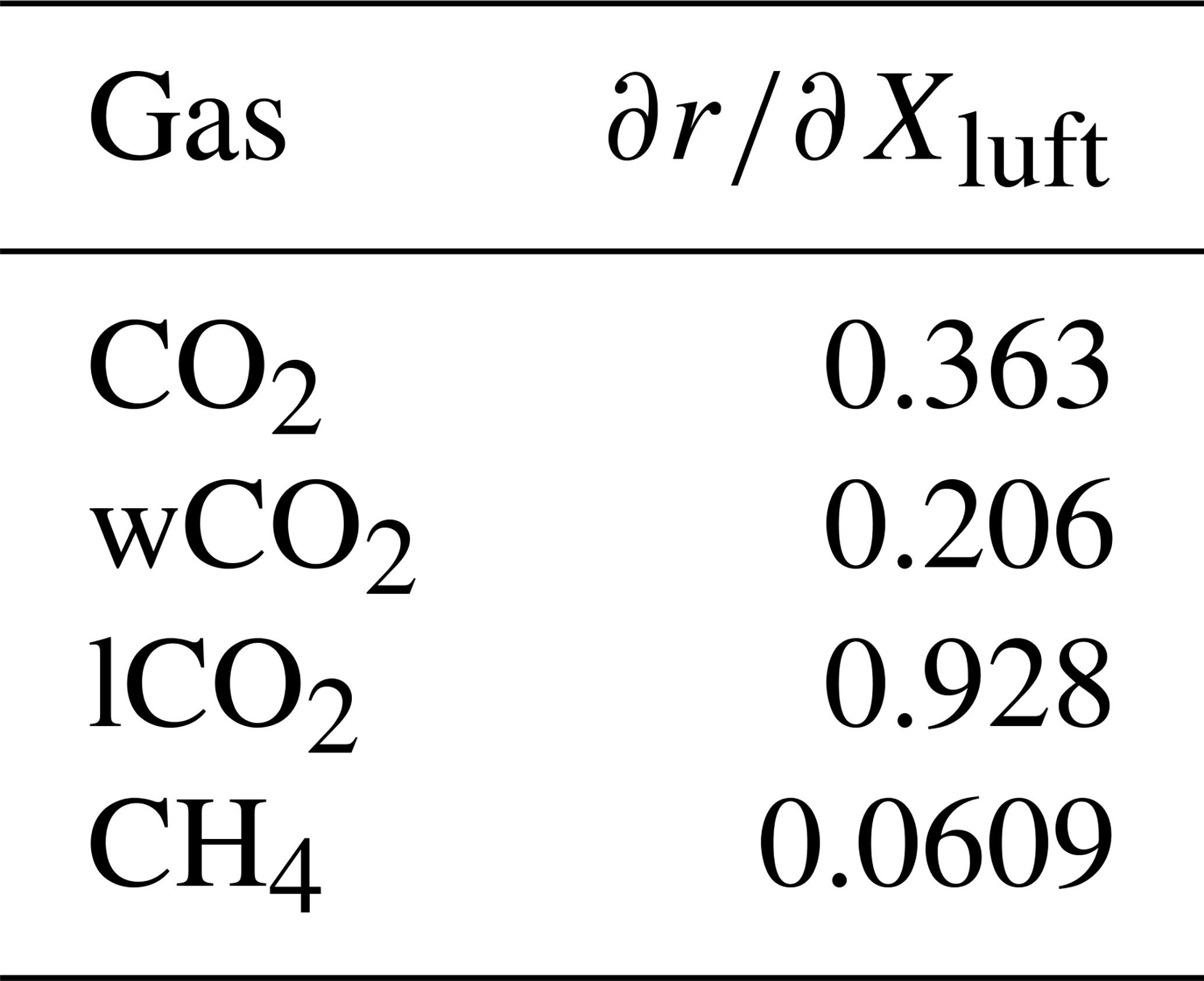
Table C7The magnitudes of each uncertainty component for the AICF comparison. As in Table 5, the first number in each column is the overall contribution of that term to the AICF according to formal error propagation, and the number in parentheses is the simple mean across all the TCCON to in situ comparisons. The units for each gas's error values are given in the first column.
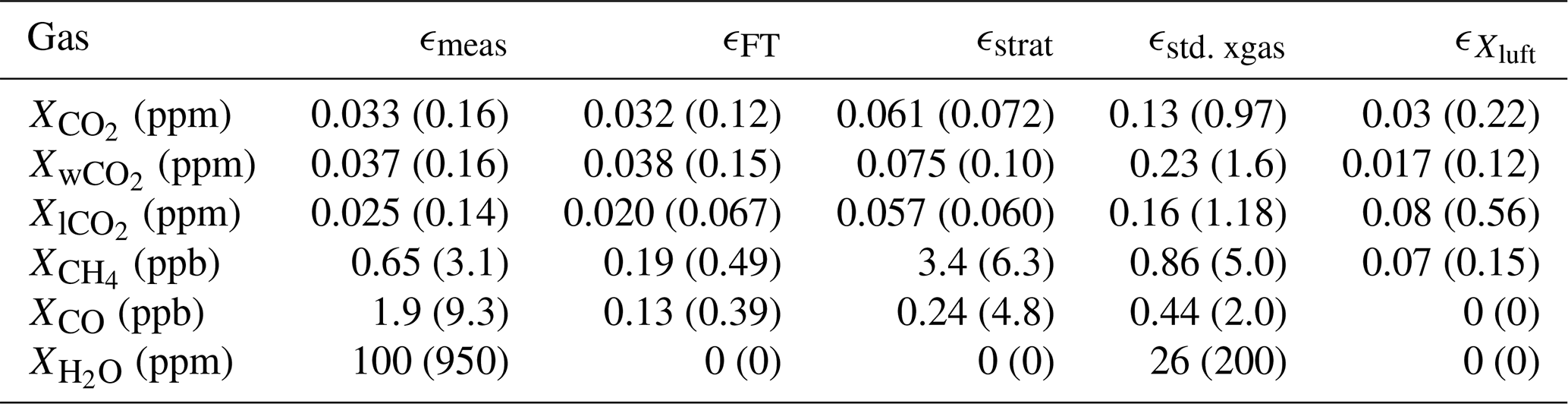
-
In situ measurement error (ϵmeas) accounts for the error in individual in situ measurements that make up the profiles. To be conservative, we assume the worst-case scenario with 100 % correlated error at all levels. The uncertainty in Xgas is then calculated as
where c(p) is the measured mixing ratio, and σ(p) is the uncertainty at each level. The integrals represent the pressure-weighted integration (see Eq. 10). The uncertainty values are those reported in the original data files where available or a typical value chosen in consultation with the data providers.
-
Unmeasured free troposphere (ϵFT) accounts for uncertainty due to the portion of the free troposphere not measured by a given profile. For each profile, we first calculate σobs,FT, the standard deviation of measurements above 750 hPa and below the tropopause (as determined by GEOS FP-IT meteorology). We then create a perturbed profile,
which adds this standard deviation to interpolated or extrapolated levels above the top of the measured profile. The uncertainty in Xgas is calculated as
This error will be zero for profiles that do not require extrapolation or interpolation to reach the stratospheric overworld (i.e., altitudes with potential temperature ≥380 K).
-
Bias in stratospheric prior (ϵstrat) represents expected bias in the column from the use of GGG2020 priors for levels in the stratosphere. This uses the retrieved vs. prior HF column as a proxy for error in the stratospheric prior. As discussed in Sect. 8.3.3, HF is predominately found in the stratosphere; thus, the difference between the retrieved and prior HF columns gives information about whether the stratospheric profile was biased high or low. We calculate the bias as
The derivative has to be calculated for each gas. For CO2, we use 8.09×10³, which was derived from East Trout Lake TCCON data by comparing prior and posterior wCO2 and HF columns. East Trout Lake is positioned to see significant stratospheric variability due to the polar vortex, and wCO2 is the GGG2020 CO2 product with enhanced sensitivity to the stratosphere. For CH4, this is drawn from the CH4:HF slopes used in the GGG2020 priors (Laughner et al., 2023).
AirCore profiles are treated specially as they always reach into the stratosphere. For these profiles, we create a perturbed profile, c′(p), where the levels in the stratosphere filled by the GGG2020 priors have the difference between the top of the AirCore profile and the corresponding level in the prior added to them. The difference between the integral of these profiles becomes the stratospheric error. Mathematically, that is
-
Random error in TCCON Xgas value (ϵstd. xgas) represents random error in the TCCON observations. Because we require at least 30 TCCON observations coincident with a profile for a valid comparison, we use twice the standard deviation among those coincident observations as the metric of random error. The coincidence windows vary between 2 and 6 h wide; thus, the standard deviation likely includes some true change in the data and can therefore be considered to be conservative.
-
Bias in TCCON derived from Xluft () represents bias in retrieved Xgas values resulting from instrument hardware issues diagnosed from deviations in Xluft from the nominal network value (0.999; see Sect. 8.3). The bias is calculated as
Here, Xluft,median and Xgas,median are the median values of TCCON Xluft and the target Xgas across the 30+ coincident observations for the comparison; 0.999 is the nominal value of Xluft that represents a well-operating instrument. The value is how the TCCON in situ ratio changes with Xluft and was derived for , , , and by an unweighted robust fit through similar plots of TCCON in situ ratio vs. Xluft as in Fig. 16 but with TCCON retrievals that used the standard trace gas priors instead of custom ones built from the in situ profiles. The values used are given in Table C6.
With regard to full error calculation, as the error terms include a mix of random (ϵmeas, ϵFT, ϵstd. xgas) and systematic (ϵstrat, ) errors, the in situ and TCCON total errors are calculated as
The first term in the second equation is written as a root of a square to indicate that, if additional random TCCON error terms were to be added in the future, they should add in quadrature. The uncertainty in the TCCON in situ ratio () follows standard error propagation ():
Note that Eq. (C12) is applied to each individual TCCON in situ comparison, while the statistics in Table 5 are averaged over all the comparisons for a given gas. Therefore, the values of ϵin situ, ϵmeas, ϵFT, and ϵstrat in Table 5 do not directly relate to each other through Eq. (C12). As noted in the caption for Table 5, the non-parenthetical values in the last four columns formally propagate the error from the individual comparisons, such that the values shown in the table (which we will denote generally as ϵformal) are calculated from the individual comparisons' values with
where ϵindiv,i denotes individual comparisons' error values, and n is the number of individual observations. Conversely, the parenthetical numbers in Table 5 give the simple mean – i.e.,
For Fig. 19, we constructed N2O profiles to compare TCCON against using NOAA surface data. This approach takes advantage of how well mixed N2O is in the troposphere to build a large set of comparison. The approach, in detail, is as follows.
The TCCON vs. in situ comparison shown in Fig. 19 calculates an in situ from N2O profiles using Eq. (9), as with the other Xgas quantities in Sect. 8.3. These N2O profiles are constructed using the NOAA surface N2O VMR from the surface to the tropopause and the GGG2020 N2O prior for levels with potential temperature greater than 380 K, linearly interpolating the N2O VMR with respect to potential temperature between the tropopause and the 380 K level.
For the tropospheric N2O VMRs, we obtained monthly average NOAA global N2O data from https://gml.noaa.gov/hats/combined/N2O.html (last access: 10 May 2021). For sites at latitudes north of 23° N or south of 23° S, we use the northern and southern hemispheric averages, respectively (GML_NH_N2O and GML_SH_N2O in the combined NOAA N2O file). For equatorial latitudes between 23° S and 23° N, we used the average of the Mauna Loa and American Samoa N2O data (GML_mlo_N2O and GML_smo_N2O in the combined file). For each comparison point in Fig. 19, we used the N2O VMR from that month as the tropospheric VMR of the profile.
The comparisons selected for Fig. 19 meet the following criteria:
-
The difference between the prior and posterior HF column must be molec. cm−2 in magnitude. Since HF is almost entirely in the stratosphere, this limits the comparisons to cases where the GGG2020 prior stratospheric profiles are reasonably accurate, thus limiting error in the in situ from an incorrectly assumed stratosphere
-
Xluft must be in the range [0.996,1.002). This ensures that we are considering data from when the TCCON instrument was well aligned, as discussed in Sect. 8.3.1
-
FVSI must be ≤0.05. This limits the comparison to mostly cloud-free observations.
E1 Trends in O2 dry mole fraction from trends in
The derivation of Eq. (12) begins from the definition of :
where
-
and are the number of moles of O2 and CO2, respectively;
-
N is the number of moles of gases other than O2 or CO2 in H2O-free air; and
-
Ntot (used below) is .
Defining , taking the derivative of with respect to , and simplifying gives
recognizing that and , as well as converting the derivative to a ratio of small but finite differences (represented by δ in place of ∂), give
Finally, to convert into terms of and , we start by defining
and
as well as . Substituting this and from Eq. (E5) in Eq. (E6) and rearranging gives
Substituting Eq. (E7) in Eq. (E4) yields the final version of Eq. (12).
E2 O2 dry mole fraction from O2/N2 data
Measurements of atmospheric O2 concentration are commonly reported as 10−6 relative deviations in the O2 N2 ratio (denoted and given in units of per meg) to avoid the complexities of dilution effects from changes in CO2 and other trace species in the O2 dry mole fraction. To convert from available measurements of trends in , we must convert to units of ppm and account for the diluting effect of trends in CO2. The equation for the black line in Fig. 18, based on Scripps and NOAA global mean CO2 data, is slightly different from Eq. (12). As above, the derivation starts with Eq. (E1), but now, since we have measured values for the change in and , our change in will instead be
In this case, both and are 0 since we have measurements of both O2 and CO2 and therefore can treat their changes as orthogonal. This leads to the following expressions for the derivatives in Eq. (E8):
Inserting these into Eq. (E8) gives
can be expressed in terms of values by using the definition of (Keeling et al., 1998):
assuming that the amount of N2 in the atmosphere does not change. Multiplying this definition by gives
can be expressed as in Eq. (E7), except with α=0 (again, this is because we have measurements of dry mole fractions of CO2 and O2). The final equation used for the best estimate line in Fig. 18 is therefore
where is the 0.209341 value obtained in Sect. 8.3.2 by adjusting Aoki et al. (2019). As noted in Sect. 8.3.2, the data used are a weighted average of the ALT, LJO, and CGO sites, with weights of , , and , respectively. Note that the NOAA global mean CO2 (rather than TCCON ) is used for and in this equation.
JLL led the development of the new air mass correction (Sect. 8.1), window-to-window averaging (Sect. 8.2), in situ scaling (Sect. 8.3), and miscellaneous changes in Sect. 3. GCT is the main developer of GGG. JM developed the non-Voigt treatment of the spectral line shape (Sect. 6.2). CP contributed to the development of the phase correction update (Sect. 4.2). SR developed the new retrieval grid (Sect. 5.1), meteorological resampler (Sect. 5.2), and netCDF writer. DW carried out the sensitivity tests (Sect. 9). DW, CMR, GCT, POW, and JLL conducted the O2 study in Sect. 6.3. JFB is a key developer of I2S. DWTG contributed to various aspects of GGG2020 development. PH, RK, and MKS first diagnosed the nonlinearity issue from Sect. 4.1 and developed a correction methodology. RFK and BBS consulted on the approaches to parameterize the change in O2 dry mole fraction (Sect. 8.3.2). MK performed tests of the phase correction threshold (Sect. 4.2) and choices of NCBFs (Sect. 7). CMR, ND, PJ, DP, MR, SR, MKS, YT, and DW all participated in a beta test of GGG2020. NMD, JG, BH, PJ, IM, HO, CP, JN, DP, MR, SR, EM, KS, CMR, MKS, KS, RS, YT, VV, DW, and MZ provided data used to derive the corrections in Sect. 8.1 and 8.2. BCB, BBS, HC, RK, YC, XL, TL, KM, JM, HR, CR, and SCW provided the in situ data used in Sect. 8.3. POW provided input to all elements of this work. All the authors reviewed the paper.
The contact author has declared that none of the authors has any competing interests.
Publisher's note: Copernicus Publications remains neutral with regard to jurisdictional claims made in the text, published maps, institutional affiliations, or any other geographical representation in this paper. While Copernicus Publications makes every effort to include appropriate place names, the final responsibility lies with the authors.
The authors gratefully acknowledge the use of GNU Parallel (Tange, 2011) in the GGG processing. The authors also thank James Abshire for providing the CO2 data used in deriving the in situ correction (Sect. 8.3). A portion of this research was carried out at the Jet Propulsion Laboratory (JPL), California Institute of Technology, under a contract with NASA (80NM0018D0004). Government sponsorship is acknowledged. Support for Caltech TCCON sites and partial support for Joshua L. Laughner, Matthäus Kiel, Coleen M. Roehl, and Paul O. Wennberg were provided by NASA grants NNX17AE15G and 80NSSC22K1066. Material from Britton B. Stephens and Ralph F. Keeling is based upon work supported by the National Center for Atmospheric Research, which is a major facility sponsored by the National Science Foundation under Cooperative Agreement No. 1852977.
Markus Rettinger and Ralf Sussmann acknowledge funding by the German Helmholtz Research Program “Changing Earth – Sustaining our Future” within the Research Field “Earth and Environment”. The Paris TCCON site has received funding from Sorbonne Université, the French research center CNRS, and the French space agency CNES. The Cyprus TCCON site and AirCore flights have received funding from the European Union’s Horizon 2020 research and innovation program under grant agreement no. 856612 and from the Cyprus Government. The TCCON site at Réunion Island has been operated by the Royal Belgian Institute for Space Aeronomy with financial support since 2014 by the EU project ICOS-INIWRE (grant agreement no. 313169), the ministerial decree for ICOS (grant nos. FR/35/IC1 to FR/35/C6), the ESFRI-FED ICOS-BE project (grant no. EF/211/ICOS-BE), and local activities supported by LACy/UMR8105 and by OSU-R/UMS3365 – Université de La Réunion. The Eureka TCCON measurements were made at the Polar Environment Atmospheric Research Laboratory (PEARL) by the Canadian Network for the Detection of Atmospheric Change (CANDAC), primarily supported by the Natural Sciences and Engineering Research Council of Canada, Environment and Climate Change Canada, and the Canadian Space Agency. TCCON sites at Tsukuba, Rikubetsu, and Burgos are supported in part by the GOSAT series project. Burgos is supported in part by the Energy Development Corporation Philippines.
This research has been supported by the National Aeronautics and Space Administration (contract no. 80NM0018D0004, grant nos. NNX17AE15G, and 80NSSC22K1066), the Horizon 2020 (grant no. EMME-CARE – Eastern Mediterranean and Middle East – Climate and Atmosphere Research Centre (856612)), the Seventh Framework Programme FP7 Cooperation (grant no. 313169), and the Belgian Federal Science Policy Office (grant nos. FR/35/IC1 to FR/35/C6 and EF/211/ICOS-BE).
This paper was edited by David Carlson and reviewed by Denis Jouglet, Gretchen Keppel-Aleks, and one anonymous referee.
Abrams, M. C., Toon, G. C., and Schindler, R. A.: Practical example of the correction of Fourier-transform spectra for detector nonlinearity, Appl. Optics, 33, 6307–6314, https://doi.org/10.1364/AO.33.006307, 1994. a
Allen, D. R. and Nakamura, N.: Tracer Equivalent Latitude: A Diagnostic Tool for Isentropic Transport Studies, J. Atmos. Sci., 60, 287–304, https://doi.org/10.1175/1520-0469(2003)060<0287:TELADT>2.0.CO;2, 2003. a
Andrews, A.: Technical Procedure: Analysis of Carbon Monoxide in Air, https://www.gml.noaa.gov/ccl/docs/TP_analysis_CO_v2.0.pdf (last access: 13 September 2022), 2019. a
Aoki, N., Ishidoya, S., Matsumoto, N., Watanabe, T., Shimosaka, T., and Murayama, S.: Preparation of primary standard mixtures for atmospheric oxygen measurements with less than 1 µmol mol−1 uncertainty for oxygen molar fractions, Atmos. Meas. Tech., 12, 2631–2646, https://doi.org/10.5194/amt-12-2631-2019, 2019. a, b, c
Baier, B., Sweeney, C., Tans, P., Newberger, T., Higgs, J., Wolter, S., and NOAA Global Monitoring Laboratory: NOAA AirCore atmospheric sampling system profiles (Version 20201223), NOAA GML [data set], https://doi.org/10.15138/6AV0-MY81, 2021. a, b
Benner, D. C., Devi, V. M., Sung, K., Brown, L. R., Miller, C. E., Payne, V. H., Drouin, B. J., Yu, S., Crawford, T. J., Mantz, A. W., Smith, M. A. H., and Gamache R. R.: Line parameters including temperature dependences of air-and self-broadened line shapes of 12C16O2: 2.06-µm region, J. Mol. Spectrosc., 326, 21–47, 2016. a
Buschmann, M., Petri, C., Palm, M., Warneke, T., Notholt, J., and AWIPEV Station Engineers: TCCON data from Ny-Alesund, Svalbard, Norway, Release GGG2020R0, TCCON data archive, hosted by CaltechDATA [data set], California Institute of Technology, Pasadena, CA, USA, https://doi.org/10.14291/tccon.ggg2020.nyalesund01.R0, 2022. a
Byrne, B., Baker, D. F., Basu, S., Bertolacci, M., Bowman, K. W., Carroll, D., Chatterjee, A., Chevallier, F., Ciais, P., Cressie, N., Crisp, D., Crowell, S., Deng, F., Deng, Z., Deutscher, N. M., Dubey, M. K., Feng, S., García, O. E., Griffith, D. W. T., Herkommer, B., Hu, L., Jacobson, A. R., Janardanan, R., Jeong, S., Johnson, M. S., Jones, D. B. A., Kivi, R., Liu, J., Liu, Z., Maksyutov, S., Miller, J. B., Miller, S. M., Morino, I., Notholt, J., Oda, T., O'Dell, C. W., Oh, Y.-S., Ohyama, H., Patra, P. K., Peiro, H., Petri, C., Philip, S., Pollard, D. F., Poulter, B., Remaud, M., Schuh, A., Sha, M. K., Shiomi, K., Strong, K., Sweeney, C., Té, Y., Tian, H., Velazco, V. A., Vrekoussis, M., Warneke, T., Worden, J. R., Wunch, D., Yao, Y., Yun, J., Zammit-Mangion, A., and Zeng, N.: National CO2 budgets (2015–2020) inferred from atmospheric CO2 observations in support of the global stocktake, Earth Syst. Sci. Data, 15, 963–1004, https://doi.org/10.5194/essd-15-963-2023, 2023. a
Chen, Y., Cheng, J., Song, X., Liu, S., Sun, Y., Yu, D., and Fang, S.: Global-Scale Evaluation of XCO2 Products from GOSAT, OCO-2 and CarbonTracker Using Direct Comparison and Triple Collocation Method, Remote Sens., 14, 5635, https://doi.org/10.3390/rs14225635, 2022. a
Cooperative Global Atmospheric Data Integration Project: Multi-laboratory compilation of atmospheric carbon dioxide data for the period 1957–2018; obspack_co2_1_GLOBALVIEWplus_v5.0_2019_08_12; NOAA Earth System Research Laboratory, Global Monitoring Division, https://doi.org/10.25925/20190812, 2019. a, b, c, d
Cooperative Global Atmospheric Data Integration Project: Multi-laboratory compilation of atmospheric methane data for the period 1957-2018; obspack_ch4_1_GLOBALVIEWplus_v2.0_2020-04-24; NOAA Earth System Research Laboratory, Global Monitoring Division, https://doi.org/10.25925/20200424, 2020. a, b, c, d
Corredera, P., Hernanz, M. L., lez Herr ez, M. G., and Campos, J.: Anomalous non-linear behaviour of InGaAs photodiodes with overfilled illumination, Metrologia, 40, S150–S153, https://doi.org/10.1088/0026-1394/40/1/334, 2003. a
Crisp, D., Rosenberg, R., Chapsky, L., Keller Rodrigues, G. R., Lee, R., Merrelli, A., Osterman, G., Oyafuso, F., Pollock, R., Spiers, R., Yu, S., Zong, J., and Eldering, A.: Orbiting Carbon Observatory (OCO) – 2 & 3 Level 1B Theoretical Basis Document, Version 2.0, Rev 0, https://docserver.gesdisc.eosdis.nasa.gov/public/project/OCO/OCO_L1B_ATBD.pdf (last access: 11 January 2024), 2021. a
De Mazière, M., Sha, M. K., Desmet, F., Hermans, C., Scolas, F., Kumps, N., Zhou, M., Metzger, J.-M., Duflot, V., and Cammas, J.-P.: TCCON data from Reunion Island (La Reunion), France, Release GGG2020R0, TCCON data archive, hosted by CaltechDATA [data set], California Institute of Technology, Pasadena, CA, USA, https://doi.org/10.14291/tccon.ggg2020.reunion01.R0, 2022. a
Deutscher, N. M., Griffith, D. W. T., Bryant, G. W., Wennberg, P. O., Toon, G. C., Washenfelder, R. A., Keppel-Aleks, G., Wunch, D., Yavin, Y., Allen, N. T., Blavier, J.-F., Jiménez, R., Daube, B. C., Bright, A. V., Matross, D. M., Wofsy, S. C., and Park, S.: Total column CO2 measurements at Darwin, Australia – site description and calibration against in situ aircraft profiles, Atmos. Meas. Tech., 3, 947–958, https://doi.org/10.5194/amt-3-947-2010, 2010. a
Deutscher, N. M., Griffith, D. W., Paton-Walsh, C., Velazco, V. A., Wennberg, P. O., Blavier, J.-F., Washenfelder, R. A., Yavin, Y., Keppel-Aleks, G., Toon, G. C., Jones, N. B., Kettlewell, G. C., Connor, B. J., Macatangay, R. C., Wunch, D., Roehl, C., and Bryant, G. W.: TCCON data from Darwin (AU), Release GGG2020.R0 [data set], https://doi.org/10.14291/tccon.ggg2020.darwin01.R0, 2023a. a
Deutscher, N. M., Griffith, D. W. T., Paton-Walsh, C., Jones, N. B., Velazco, V. A., Wilson, S. R., Macatangay, R. C., Kettlewell, G. C., Buchholz, R. R., Riggenbach, M. O., Bukosa, B., John, S. S., Walker, B. T., and Nawaz, H.: TCCON data from Wollongong, Australia, Release GGG2020R0, TCCON data archive, hosted by CaltechDATA [data set], California Institute of Technology, Pasadena, CA, USA, https://doi.org/10.14291/tccon.ggg2020.wollongong01.R0, 2023b. a
Devi, V. M., Benner, D. C., Brown, L., Miller, C., and Toth, R.: Line mixing and speed dependence in CO2 at 6348 cm−1: Positions, intensities, and air-and self-broadening derived with constrained multispectrum analysis, J. Mol. Spectrosc., 242, 90–117, 2007a. a
Devi, V. M., Benner, D. C., Brown, L., Miller, C., and Toth, R.: Line mixing and speed dependence in CO2 at 6227.9 cm−1: Constrained multispectrum analysis of intensities and line shapes in the 30013← 00001 band, J. Mol. Spectrosc., 245, 52–80, 2007b. a
Devi, V. M., Benner, D. C., Sung, K., Crawford, T. J., Yu, S., Brown, L. R., Smith, M. A. H., Mantz, A. W., Boudon, V., and Ismail, S.: Self-and air-broadened line shapes in the 2ν3 P and R branches of 12CH4, J. Mol. Spectrosc., 315, 114–136, 2015. a, b
Devi, V. M., Benner, D. C., Sung, K., Brown, L. R., Crawford, T. J., Yu, S., Smith, M. A. H., Mantz, A. W., Boudon, V., and Ismail, S.: Spectral line parameters including line shapes in the 2ν3 Q branch of 12CH4, J. Quant. Spectrosc. Ra., 177, 152–169, 2016. a, b
Dubey, M., Henderson, B., Green, D., Butterfield, Z., Keppel-Aleks, G., Allen, N., Blavier, J.-F., Roehl, C., Wunch, D., and Lindenmaier, R.: TCCON data from Manaus, Brazil, Release GGG2020R0, TCCON data archive, hosted by CaltechDATA [data set], California Institute of Technology, Pasadena, CA, USA, https://doi.org/10.14291/tccon.ggg2020.manaus01.R0, 2022a. a
Dubey, M., Lindenmaier, R., Henderson, B., Green, D., Allen, N., Roehl, C., Blavier, J.-F., Butterfield, Z., Love, S., Hamelmann, J., and Wunch, D.: TCCON data from Four Corners, NM, USA, Release GGG2020R0, TCCON data archive, hosted by CaltechDATA [data set], California Institute of Technology, Pasadena, CA, USA, https://doi.org/10.14291/tccon.ggg2020.fourcorners01.R0, 2022b. a
Dubey, M. K., Parker, H. A., Wennberg, P. O., Wunch, D., Jacobson, A. R., Kawa, S. R., Keppel-Aleks, G., Basu, S., O'Dell, C., Frankenberg, C., Michalak, A. M., Baker, D. F., Christofferson, B., Restrepo-Coupe, N., Saleska, S. R., De Araujo, A. C., and Miller, J. B.: Seasonal & Daily Amazon Column CO2 & CO Observations from Ground & Space Used to Evaluate Tropical Ecosystem Models, American Geophysical Union, Fall Meeting 2016, abstract #B33C-0623, https://agu.confex.com/agu/fm16/meetingapp.cgi/Paper/189108 (last access: 22 April 2024, 2016. a
Dutton, G., Hall, B., Dlugokencky, E., Lan, X., Nance, J., and Madronich, M.: Combined Atmospheric Nitrous Oxide Dry Air Mole Fractions from the NOAA GML Halocarbons Sampling Network, 1977-2023, Version: 2023-04-13, https://doi.org/10.15138/GMZ7-2Q16, 2023. a
ESA: Copernicus CO2 Monitoring Mission Requirements Document, https://esamultimedia.esa.int/docs/EarthObservation/CO2M_MRD_v3.0_20201001_Issued.pdf (last access: 11 January 2024), 2020. a
Fleurbaey, H., Reed, Z. D., Adkins, E. M., Long, D. A., and Hodges, J. T.: High accuracy spectroscopic parameters of the 1.27 µm band of O2 measured with comb-referenced, cavity ring-down spectroscopy, J. Quant. Spectrosc. Ra., 270, 107684, https://doi.org/10.1016/j.jqsrt.2021.107684, 2021.Please provide DOI. a, b
Forman, M. L., Steel, W. H., and Vanasse, G. A.: Correction of Asymmetric Interferograms Obtained in Fourier Spectroscopy, J. Opt. Soc. Am., 56, 59–63, https://doi.org/10.1364/JOSA.56.000059, 1966. a
Fox, N. P.: Improved Near-Infrared Detectors, Metrologia, 30, 321, https://doi.org/10.1088/0026-1394/30/4/019, 1993. a
García, O. E., Schneider, M., Herkommer, B., Gross, J., Hase, F., Blumenstock, T., and Sepúlveda, E.: TCCON data from Izana (ES), Release GGG2020.R1 (Version R1), CaltechDATA [data set], https://doi.org/0.14291/tccon.ggg2020.izana01.R1, 2022. a
Gordon, I. E., Rothman, L. S., Hill, C., Kochanov, R. V., Tan, Y., Bernath, P. F., Birk, M., Boudon, V., Campargue, A., Chance, K., and Drouin, B. J. and Flaud, J.-M., Gamache, R. R., Hodges, J. T., Jacquemart, D., Perevalov, V. I., Perrin, A., Shine, K. P., Smith, M.-A. H., Tennyson, J., Toon, G. C., Tran, H., Tyuterev, V. G., Barbe, A., Császár, A. G., Devi, V. M., Furtenbacher, T., Harrison, J. J., Hartmann, J.-M., Jolly, A., Johnson, T. J., Karman, T., Kleiner, I., Kyuberis, A. A., Loos, J., Lyulin, O. M., Massie, S. T., Mikhailenko, S. N., Moazzen-Ahmadi, N., Müller, H. S. P., Naumenko, O. V., Nikitin, A. V., Polyansky, O. L., Rey, M., Rotger, M., Sharpe, S. W., Sung, K., Starikova, E., Tashkun, S. A., Auwera, J. Vander, Wagner, G., Wilzewski, J., Wcisło, P., Yu, S., and Zak, E. J.: The HITRAN2016 molecular spectroscopic database, J. Quant. Spectrosc. Ra., 203, 3–69, 2017. a
Hall, B. D., Crotwell, A. M., Kitzis, D. R., Mefford, T., Miller, B. R., Schibig, M. F., and Tans, P. P.: Revision of the World Meteorological Organization Global Atmosphere Watch (WMO/GAW) CO2 calibration scale, Atmos. Meas. Tech., 14, 3015–3032, https://doi.org/10.5194/amt-14-3015-2021, 2021. a, b
Hartmann, J.-M., Tran, H., and Toon, G. C.: Influence of line mixing on the retrievals of atmospheric CO2 from spectra in the 1.6 and 2.1 µm regions, Atmos. Chem. Phys., 9, 7303–7312, https://doi.org/10.5194/acp-9-7303-2009, 2009. a
Hase, F.: Inversion von Spurengasprofilen aus hochaufgelöstenbodengebundenen FTIR-Messungen in Absorption, Ph.D. thesis, Institut für Meteorologie und Klimaforschung, Forschungszentrum Karlsruhe GmbH, Karlsruhe, http://www.imk-asf.kit.edu/downloads/bod/disshase.pdf (last access: 22 April 2024), 2000. a
Hase, F., Blumenstock, T., and Paton-Walsh, C.: Analysis of the instrumental line shape of high-resolution Fourier transform IR spectrometers with gas cell measurements and new retrieval software, Appl. Optics, 38, 3417–3422, https://doi.org/10.1364/AO.38.003417, 1999. a, b
Hase, F., Drouin, B. J., Roehl, C. M., Toon, G. C., Wennberg, P. O., Wunch, D., Blumenstock, T., Desmet, F., Feist, D. G., Heikkinen, P., De Mazière, M., Rettinger, M., Robinson, J., Schneider, M., Sherlock, V., Sussmann, R., Té, Y., Warneke, T., and Weinzierl, C.: Calibration of sealed HCl cells used for TCCON instrumental line shape monitoring, Atmos. Meas. Tech., 6, 3527–3537, https://doi.org/10.5194/amt-6-3527-2013, 2013. a, b
Hase, F., Blumenstock, T., Dohe, S., Groß, J., and Kiel, M.: TCCON data from Karlsruhe, Germany, Release GGG2020R1, TCCON data archive, hosted by CaltechDATA [data set], California Institute of Technology, Pasadena, CA, USA, https://doi.org/10.14291/tccon.ggg2020.karlsruhe01.R1, 2022. a
Hashemi, R., Gordon, I. E., Tran, H., Kochanov, R. V., Karlovets, E. V., Tan, Y., Lamouroux, J., Ngo, N. H., and Rothman, L. S.: Revising the line-shape parameters for air-and self-broadened CO2 lines toward a sub-percent accuracy level, Journal of Quantitative Spectroscopy and Radiative Transfer, 256, 107 283, 2020. a
Hedelius, J. K., He, T.-L., Jones, D. B. A., Baier, B. C., Buchholz, R. R., Mazière, M. D., Deutscher, N. M., Dubey, M. K., Feist, D. G., Griffith, D. W. T., Hase, F., Iraci, L. T., Jeseck, P., Kiel, M., Kivi, R., Liu, C., Morino, I., Notholt, J., Oh, Y.-S., Ohyama, H., Pollard, D. F., Rettinger, M., Roche, S., Roehl, C. M., Schneider, M., Shiomi, K., Strong, K., Sussmann, R., Sweeney, C., Té, Y., Uchino, O., Velazco, V. A., Wang, W., Warneke, T., Wennberg, P. O., Worden, H. M., and Wunch, D.: Evaluation of MOPITT Version 7 joint TIR-NIR XCO retrievals with TCCON, Atmos. Meas. Tech., 12, 5547–5572, https://doi.org/10.5194/amt-12-5547-2019, 2019. a
Iraci, L., Podolske, J., Hillyard, P., Roehl, C., Wennberg, P. O., Blavier, J.-F., Landeros, J., Allen, N., Wunch, D., Zavaleta, J., Quigley, E., Osterman, G., Barrow, E., and Barney, J.: TCCON data from Indianapolis, Indiana, USA, Release GGG2020R0, TCCON data archive, hosted by CaltechDATA [data set], California Institute of Technology, Pasadena, CA, USA, https://doi.org/10.14291/tccon.ggg2020.indianapolis01.R1, 2022a. a
Iraci, L., Podolske, J., Roehl, C., Wennberg, P. O., Blavier, J.-F., Allen, N., Wunch, D., and Osterman, G.: TCCON data from Armstrong Flight Research Center, Edwards, CA, USA, Release GGG2020R0, TCCON data archive, hosted by CaltechDATA [data set], California Institute of Technology, Pasadena, CA, USA, https://doi.org/10.14291/tccon.ggg2020.edwards01.R0, 2022b. a
Karion, A., Sweeney, C., Tans, P., and Newberger, T.: AirCore: An Innovative Atmospheric Sampling System, J. Atmos. Ocean. Tech., 27, 1839–1853, https://doi.org/10.1175/2010jtecha1448.1, 2010. a
Keeler, E., Burk, K. and Kyrouac, J.: Balloon-Borne Sounding System (SONDEWNPN), Atmospheric Radiation Measurement (ARM) user facility [data set], https://doi.org/10.5439/1595321, 2001. a
Keeling, R. and Manning, A.: Studies of Recent Changes in Atmospheric O2 Content, in: Treatise on Geochemistry, Elsevier, 385–404, https://doi.org/10.1016/b978-0-08-095975-7.00420-4, 2014. a, b
Keeling, R. F., Manning, A. C., McEvoy, E. M., and Shertz, S. R.: Methods for measuring changes in atmospheric O2 concentration and their application in southern hemisphere air, J. Geophys. Res.-Atmos., 103, 3381–3397, https://doi.org/10.1029/97jd02537, 1998. a, b
Keppel-Aleks, G., Toon, G. C., Wennberg, P. O., and Deutscher, N. M.: Reducing the impact of source brightness fluctuations on spectra obtained by Fourier-transform spectrometry, Appl. Optics, 46, 4774–4779, https://doi.org/10.1364/AO.46.004774, 2007. a, b, c
Keppel-Aleks, G., Wennberg, P. O., Washenfelder, R. A., Wunch, D., Schneider, T., Toon, G. C., Andres, R. J., Blavier, J.-F., Connor, B., Davis, K. J., Desai, A. R., Messerschmidt, J., Notholt, J., Roehl, C. M., Sherlock, V., Stephens, B. B., Vay, S. A., and Wofsy, S. C.: The imprint of surface fluxes and transport on variations in total column carbon dioxide, Biogeosciences, 9, 875–891, https://doi.org/10.5194/bg-9-875-2012, 2012. a
Kiel, M., Hase, F., Blumenstock, T., and Kirner, O.: Comparison of XCO abundances from the Total Carbon Column Observing Network and the Network for the Detection of Atmospheric Composition Change measured in Karlsruhe, Atmos. Meas. Tech., 9, 2223–2239, https://doi.org/10.5194/amt-9-2223-2016, 2016a. a
Kiel, M., Wunch, D., Wennberg, P. O., Toon, G. C., Hase, F., and Blumenstock, T.: Improved retrieval of gas abundances from near-infrared solar FTIR spectra measured at the Karlsruhe TCCON station, Atmos. Meas. Tech., 9, 669–682, https://doi.org/10.5194/amt-9-669-2016, 2016b. a
Kivi, R. and Heikkinen, P.: Fourier transform spectrometer measurements of column CO2 at Sodankylä, Finland, Geosci. Instrum. Method. Data Syst., 5, 271–279, https://doi.org/10.5194/gi-5-271-2016, 2016. a
Kivi, R., Heikkinen, P., and Kyro, E.: TCCON data from Sodankyla, Finland, Release GGG2020R0, TCCON data archive, hosted by CaltechDATA [data set], California Institute of Technology, Pasadena, CA, USA, https://doi.org/10.14291/tccon.ggg2020.sodankyla01.R0, 2022. a
Lan, X., Dlugokencky, E., Mund, J., Crotwell, A., Crotwell, M., Moglia, E., Madronich, M., Neff, D., and Thoning, K.: Atmospheric Methane Dry Air Mole Fractions from the NOAA GML Carbon Cycle Cooperative Global Air Sampling Network, 1983–2021, Version: 2022-11-21, https://doi.org/10.15138/VNCZ-M766, 2022a. a
Lan, X., Dlugokencky, E., Mund, J., Crotwell, A., Crotwell, M., Moglia, E., Madronich, M., Neff, D., and Thoning, K.: Atmospheric Carbon Dioxide Dry Air Mole Fractions from the NOAA GML Carbon Cycle Cooperative Global Air Sampling Network, 1968–2021, Version: 2022-11-21, https://doi.org/10.15138/wkgj-f215, 2022b. a
Lan, X., Dlugokencky, E., Mund, J., Crotwell, A., Crotwell, M., Moglia, E., Madronich, M., Neff, D., and Thoning, K.: Atmospheric Nitrous Oxide Dry Air Mole Fractions from the NOAA GML Carbon Cycle Cooperative Global Air Sampling Network, 1997–2021, Version: 2022-11-21, https://doi.org/10.15138/9N0H-ZH07, 2022c. a
Lan, X., Tans, P., and Thoning, K.: Trends in globally-averaged CO2 determined from NOAA Global Monitoring Laboratory measurements, Version 2023-04, https://doi.org/10.15138/9N0H-ZH07, 2023. a, b
Laughner, J. L., Roche, S., Kiel, M., Toon, G. C., Wunch, D., Baier, B. C., Biraud, S., Chen, H., Kivi, R., Laemmel, T., McKain, K., Quéhé, P.-Y., Rousogenous, C., Stephens, B. B., Walker, K., and Wennberg, P. O.: A new algorithm to generate a priori trace gas profiles for the GGG2020 retrieval algorithm, Atmos. Meas. Tech., 16, 1121–1146, https://doi.org/10.5194/amt-16-1121-2023, 2023. a, b, c, d, e, f, g, h, i, j
Liu, C., Wang, W., and Sun, Y.: TCCON data from Hefei, China, Release GGG2020R0, TCCON data archive, hosted by CaltechDATA [data set], California Institute of Technology, Pasadena, CA, USA, https://doi.org/10.14291/tccon.ggg2020.hefei01.R0, 2022. a
Lorente, A., Borsdorff, T., Martinez-Velarte, M. C., Butz, A., Hasekamp, O. P., Wu, L., and Landgraf, J.: Evaluation of the methane full-physics retrieval applied to TROPOMI ocean sun glint measurements, Atmos. Meas. Tech., 15, 6585–6603, https://doi.org/10.5194/amt-15-6585-2022, 2022. a
Lucchesi, R.: File Specification for GEOS-5 FP-IT (forward processing for instrument teams), Tech. rep., NASA Goddard Space Flight Center, Greenbelt, MD, USA, https://gmao.gsfc.nasa.gov/pubs/docs/Lucchesi865.pdf (last access: 13 October 2020), 2015. a, b
Martínez-Alonso, S., Deeter, M. N., Baier, B. C., McKain, K., Worden, H., Borsdorff, T., Sweeney, C., and Aben, I.: Evaluation of MOPITT and TROPOMI carbon monoxide retrievals using AirCore in situ vertical profiles, Atmos. Meas. Tech., 15, 4751–4765, https://doi.org/10.5194/amt-15-4751-2022, 2022. a
Mendonca, J., Strong, K., Toon, G., Wunch, D., Sung, K., Deutscher, N., Griffith, D., and Franklin, J.: Improving atmospheric CO2 retrievals using line mixing and speed-dependence when fitting high-resolution ground-based solar spectra, J. Mol. Spectrosc., 323, 15–27, https://doi.org/10.1016/j.jms.2016.01.007, 2016. a
Mendonca, J., Strong, K., Sung, K., Devi, V., Toon, G., Wunch, D., and Franklin, J.: Using high-resolution laboratory and ground-based solar spectra to assess CH4 absorption coefficient calculations, J. Quant. Spectrosc. Ra., 190, 48–59, 2017. a
Mendonca, J., Strong, K., Wunch, D., Toon, G. C., Long, D. A., Hodges, J. T., Sironneau, V. T., and Franklin, J. E.: Using a speed-dependent Voigt line shape to retrieve O2 from Total Carbon Column Observing Network solar spectra to improve measurements of XCO2, Atmos. Meas. Tech., 12, 35–50, https://doi.org/10.5194/amt-12-35-2019, 2019. a, b, c
Mertz, L.: Transformations in optics, John Wiley and Sons, Inc., ISBN-13 978-0471596400, 1965. a
Mertz, L.: Auxiliary computation for Fourier spectrometry, Infrared Phys., 7, 17–23, https://doi.org/10.1016/0020-0891(67)90026-7, 1967. a
Miloshevich, L. M., Paukkunen, A., Vömel, H., and Oltmans, S. J.: Development and Validation of a Time-Lag Correction for Vaisala Radiosonde Humidity Measurements, J. Atmos. Ocean. Tech., 21, 1305–1327, https://doi.org/10.1175/1520-0426(2004)021<1305:davoat>2.0.co;2, 2004. a
Miloshevich, L. M., Vömel, H., Whiteman, D. N., Lesht, B. M., Schmidlin, F. J., and Russo, F.: Absolute accuracy of water vapor measurements from six operational radiosonde types launched during AWEX-G and implications for AIRS validation, J. Geophys. Res., 111, D09S10, https://doi.org/10.1029/2005jd006083, 2006. a
Morino, I., Ohyama, H., Hori, A., and Ikegami, H.: TCCON data from Rikubetsu, Hokkaido, Japan, Release GGG2020R0, TCCON data archive, hosted by CaltechDATA [data set], California Institute of Technology, Pasadena, CA, USA, https://doi.org/10.14291/tccon.ggg2020.rikubetsu01.R0, 2022a. a
Morino, I., Ohyama, H., Hori, A., and Ikegami, H.: TCCON data from Tsukuba, Ibaraki, Japan, 125HR, Release GGG2020R0, TCCON data archive, hosted by CaltechDATA [data set], California Institute of Technology, Pasadena, CA, USA, https://doi.org/10.14291/tccon.ggg2020.tsukuba02.R0, 2022b. a
Morino, I., Velazco, V. A., Hori, A., Uchino, O., and Griffith, D. W. T.: TCCON data from Burgos, Philippines, Release GGG2020R0, TCCON data archive, hosted by CaltechDATA [data set], California Institute of Technology, Pasadena, CA, USA, https://doi.org/10.14291/tccon.ggg2020.burgos01.R0, 2022c. a
National Academies of Sciences, Engineering, and Medicine: Thriving on Our Changing Planet: A Decadal Strategy for Earth Observation from Space, The National Academies Press, Washington, DC, https://doi.org/10.17226/24938, 2018. a
Notholt, J., Petri, C., Warneke, T., Deutscher, N., Buschmann, M., Weinzierl, C., Macatangay, R., and Grupe, P.: TCCON data from Bremen, Germany, Release GGG2020R0, TCCON data archive, hosted by CaltechDATA [data set], California Institute of Technology, Pasadena, CA, USA, https://doi.org/10.14291/tccon.ggg2020.bremen01.R0, 2022. a
Parker, H. A., Laughner, J. L., Toon, G. C., Wunch, D., Roehl, C. M., Iraci, L. T., Podolske, J. R., McKain, K., Baier, B. C., and Wennberg, P. O.: Inferring the vertical distribution of CO and CO2 from TCCON total column values using the TARDISS algorithm, Atmos. Meas. Tech., 16, 2601–2625, https://doi.org/10.5194/amt-16-2601-2023, 2023. a
Peiro, H., Crowell, S., and Moore III, B.: Optimizing 4 years of CO2 biospheric fluxes from OCO-2 and in situ data in TM5: fire emissions from GFED and inferred from MOPITT CO data, Atmos. Chem. Phys., 22, 15817–15849, https://doi.org/10.5194/acp-22-15817-2022, 2022. a
Petri, C., Vrekoussis, M., Rousogenous, C., Warneke, T., Sciare, J., and Notholt, J.: TCCON data from Nicosia, Cyprus, Release GGG2020R1, TCCON data archive, hosted by CaltechDATA [data set], California Institute of Technology, Pasadena, CA, USA, https://doi.org/10.14291/tccon.ggg2020.nicosia01.R1, 2023. a
Pollard, D., Robinson, J., and Shiona, H.: TCCON data from Lauder, New Zealand, 125HR, Release GGG2020R0, TCCON data archive, hosted by CaltechDATA [data set], California Institute of Technology, Pasadena, CA, USA, https://doi.org/10.14291/tccon.ggg2020.lauder03.R0, 2022. a
Roche, S.: Measurements of Greenhouse Gases from Near-infrared Solar Absorption Spectra, Ph.D. thesis, University of Toronto, http://hdl.handle.net/1807/108784 (last access: 22 April 2024), 2021. a, b
Rodgers, C. D.: Inverse Methods for Atmospheric Sounding Theory and Practice, World Scientific Publishing Co. Pte. Ltd., ISBN-13 978-9810227401, 2000. a
Saad, K. M., Wunch, D., Toon, G. C., Bernath, P., Boone, C., Connor, B., Deutscher, N. M., Griffith, D. W. T., Kivi, R., Notholt, J., Roehl, C., Schneider, M., Sherlock, V., and Wennberg, P. O.: Derivation of tropospheric methane from TCCON CH4 and HF total column observations, Atmos. Meas. Tech., 7, 2907–2918, https://doi.org/10.5194/amt-7-2907-2014, 2014. a, b, c, d, e
Saad, K. M., Wunch, D., Deutscher, N. M., Griffith, D. W. T., Hase, F., De Mazière, M., Notholt, J., Pollard, D. F., Roehl, C. M., Schneider, M., Sussmann, R., Warneke, T., and Wennberg, P. O.: Seasonal variability of stratospheric methane: implications for constraining tropospheric methane budgets using total column observations, Atmos. Chem. Phys., 16, 14003–14024, https://doi.org/10.5194/acp-16-14003-2016, 2016. a, b, c
Schuldt, K. N., Mund, J., Luijkx, I. T., Aalto, T., Abshire, J. B., Aikin, K., Arlyn Andrews, Aoki, S., Apadula, F., Baier, B., Bakwin, P., Bartyzel, J., Bentz, G., Bergamaschi, P., Beyersdorf, A., Biermann, T., Biraud, S. C., and Boenisc: Multi-laboratory compilation of atmospheric carbon dioxide data for the period 1957–2020; obspack_co2_1_GLOBALVIEWplus_v7.0_2021-08-18, https://doi.org/10.25925/20210801, 2021. a
Scripps O2 Program: Flask O2/N2 data from the Alert, NWT, Canada; La Jolla Pier, California; and Cape Grim, Australia stations, https://scrippso2.ucsd.edu/data.html (last access: 27 October 2022), 2022. a
Sha, M. K., De Mazière, M., Notholt, J., Blumenstock, T., Chen, H., Dehn, A., Griffith, D. W. T., Hase, F., Heikkinen, P., Hermans, C., Hoffmann, A., Huebner, M., Jones, N., Kivi, R., Langerock, B., Petri, C., Scolas, F., Tu, Q., and Weidmann, D.: Intercomparison of low- and high-resolution infrared spectrometers for ground-based solar remote sensing measurements of total column concentrations of CO2, CH4, and CO, Atmos. Meas. Tech., 13, 4791–4839, https://doi.org/10.5194/amt-13-4791-2020, 2020. a
Sherlock, V., Connor, B., Robinson, J., Shiona, H., Smale, D., and Pollard, D.: TCCON data from Lauder, New Zealand, 120HR, Release GGG2020R0, TCCON data archive, hosted by CaltechDATA [data set], California Institute of Technology, Pasadena, CA, USA, https://doi.org/10.14291/tccon.ggg2020.lauder01.R0, 2022a. a
Sherlock, V., Connor, B., Robinson, J., Shiona, H., Smale, D., and Pollard, D.: TCCON data from Lauder, New Zealand, 125HR, Release GGG2020R0, TCCON data archive, hosted by CaltechDATA [data set], California Institute of Technology, Pasadena, CA, USA, https://doi.org/10.14291/tccon.ggg2020.lauder02.R0, 2022b. a
Shiomi, K., Kawakami, S., Ohyama, H., Arai, K., Okumura, H., Ikegami, H., and Usami, M.: TCCON data from Saga, Japan, Release GGG2020R0, TCCON data archive, hosted by CaltechDATA [data set], California Institute of Technology, Pasadena, CA, USA, https://doi.org/10.14291/tccon.ggg2020.saga01.R0, 2022. a
Strong, K., Roche, S., Franklin, J., Mendonca, J., Lutsch, E., Weaver, D., Fogal, P., Drummond, J., Batchelor, R., and Lindenmaier, R.: TCCON data from Eureka, Canada, Release GGG2020R0, TCCON data archive, hosted by CaltechDATA [data set], California Institute of Technology, Pasadena, CA, USA, https://doi.org/10.14291/tccon.ggg2020.eureka01.R0, 2022. a
Sussmann, R. and Rettinger, M.: TCCON data from Garmisch, Germany, Release GGG2020R0, TCCON data archive, hosted by CaltechDATA [data set], California Institute of Technology, Pasadena, CA, USA, https://doi.org/10.14291/tccon.ggg2020.garmisch01.R0, 2023. a
Sweeney, C., McKain, K., Higgs, J., Wolter, S., Crotwell, A., Neff, D., Dlugokencky, E., Lang, P., Novelli, P., Mund, J., Moglia, E., and Crotwell, M.: NOAA Carbon Cycle and Greenhouse Gases Group aircraft-based measurements of CO2, CH4, CO, N2O, H2 & SF6 in flask-air samples taken since 1992, NOAA Earth System Research Laboratory, Global Monitoring Division, https://doi.org/10.7289/V5N58JMF, 2018. a, b
Tange, O.: GNU Parallel – The Command-Line Power Tool, ;login: The USENIX Magazine, February, 42–47, https://www.gnu.org/software/parallel/ (last access: 22 April 2024), 2011. a
Tans, P.: System and method for providing vertical profile measurements of atmospheric gases., U.S. Patent 7,597,014, filed 15 Aug 2006, issued 6 Oct 2009, 2009. a
Te, Y., Jeseck, P., and Janssen, C.: TCCON data from Paris, France, Release GGG2020R0, TCCON data archive, hosted by CaltechDATA [data set], California Institute of Technology, Pasadena, CA, USA, https://doi.org/10.14291/tccon.ggg2020.paris01.R0, 2022. a
Toon, G.: Atmospheric Non-Voigt Line List for the TCCON 2020 Data Release (GGG2020.R0), CaltechDATA [data set], https://doi.org/10.14291/TCCON.GGG2020.ATMNV.R0, 2022a. a
Toon, G.: Solar Line List for the TCCON 2020 Data Release (GGG2020.R0), CaltechDATA [data set], https://doi.org/10.14291/TCCON.GGG2020.SOLAR.R0, 2022b. a
Toon, G.: Atmospheric Voigt Line List for the TCCON 2020 Data Release (GGG2020.R0), CaltechDATA [data set], https://doi.org/10.14291/TCCON.GGG2020.ATM.R0, 2022c. a
Toon, G.: TCCON/GGG – GGG2020, CaltechDATA [code], https://doi.org/10.14291/tccon.ggg2020.stable.R0, 2023. a
Toon, G. C., Blavier, J.-F., Sung, K., Rothman, L. S., and Gordon, I.: HITRAN spectroscopy evaluation using solar occultation FTIR spectra, J. Quant. Spectrosc. Ra., 182, 324–336, https://doi.org/10.1016/j.jqsrt.2016.05.021, 2016. a
Total Carbon Column Observing Network (TCCON) Team: 2020 TCCON Data Release (GGG2020), CaltechDATA [data set], https://doi.org/10.14291/TCCON.GGG2020, 2022. a, b, c
The TCCON community: The Total Carbon Column Observing Network Wiki, https://tccon-wiki.caltech.edu, last access: 22 April 2024. a
Tran, D., Delahaye, T., Armante, R., Hartmann, J.-M., Mondelain, D., Campargue, A., Fleurbaey, H., Hodges, J., and Tran, H.: Validation of spectroscopic data in the 1.27 µm spectral region by comparisons with ground-based atmospheric measurements, J. Quant. Spectrosc. Ra., 261, 107495, https://doi.org/10.1016/j.jqsrt.2020.107495, 2021. a
Tran, D. D., Tran, H., Vasilchenko, S., Kassi, S., Campargue, A., and Mondelain, D.: High sensitivity spectroscopy of the O2 band at 1.27 µm:(II) air-broadened line profile parameters, J. Quant. Spectrosc. Ra, 240, 106673, https://doi.org/10.1016/j.jqsrt.2019.106673, 2020. a, b
Tran, H., Ngo, N. H., and Hartmann, J.-M.: Efficient computation of some speed-dependent isolated line profiles, J. Quant. Spectrosc. Ra., 129, 199–203, 2013. a, b
Wang, Z., Deutscher, N. M., Warneke, T., Notholt, J., Dils, B., Griffith, D. W. T., Schmidt, M., Ramonet, M., and Gerbig, C.: Retrieval of tropospheric column-averaged CH4 mole fraction by solar absorption FTIR-spectrometry using N2O as a proxy, Atmos. Meas. Tech., 7, 3295–3305, https://doi.org/10.5194/amt-7-3295-2014, 2014. a, b
Warneke, T., Messerschmidt, J., Notholt, J., Weinzierl, C., Deutscher, N., Petri, C., Grupe, P., Vuillemin, C., Truong, F., Schmidt, M., Ramonet, M., and Parmentier, E.: TCCON data from Orleans, France, Release GGG2020R0, TCCON data archive, hosted by CaltechDATA [data set], California Institute of Technology, Pasadena, CA, USA, https://doi.org/10.14291/tccon.ggg2020.orleans01.R0, 2022. a
Washenfelder, R. A., Wennberg, P. O., and Toon, G. C.: Tropospheric methane retrieved from ground-based near-IR solar absorption spectra, Geophys. Res. Lett., 30, 2226, https://doi.org/10.1029/2003GL017969, 2003. a, b, c
Weidmann, D., Brownsword, R., and Doniki, S.: TCCON data from Harwell, Oxfordshire (UK), Release GGG2020.R0, CaltechDATA [data set], https://doi.org/10.14291/tccon.ggg2020.harwell01.R0, 2023. a
Wennberg, P. O., Roehl, C., Blavier, J.-F., Wunch, D., Landeros, J., and Allen, N.: TCCON data from Jet Propulsion Laboratory, Pasadena, California, USA, Release GGG2020R0, TCCON data archive, hosted by CaltechDATA [data set], California Institute of Technology, Pasadena, CA, USA, https://doi.org/10.14291/tccon.ggg2020.jpl02.R0, 2022a. a
Wennberg, P. O., Roehl, C., Wunch, D., Toon, G. C., Blavier, J.-F., Washenfelder, R., Keppel-Aleks, G., Allen, N., and Ayers, J.: TCCON data from Park Falls, Wisconsin, USA, Release GGG2020R1, TCCON data archive, hosted by CaltechDATA [data set], California Institute of Technology, Pasadena, CA, USA, https://doi.org/10.14291/tccon.ggg2020.parkfalls01.R1, 2022b. a
Wennberg, P. O., Wunch, D., Roehl, C., Blavier, J.-F., Toon, G. C., and Allen, N.: TCCON data from California Institute of Technology, Pasadena, California, USA, Release GGG2020R0, TCCON data archive, hosted by CaltechDATA [data set], California Institute of Technology, Pasadena, CA, USA, https://doi.org/10.14291/tccon.ggg2020.pasadena01.R0, 2022c. a
Wennberg, P. O., Wunch, D., Roehl, C., Blavier, J.-F., Toon, G. C., Allen, N., Dowell, P., Teske, K., Martin, C., and Martin, J.: TCCON data from Lamont, Oklahoma, USA, Release GGG2020R0, TCCON data archive, hosted by CaltechDATA [data set], California Institute of Technology, Pasadena, CA, USA, https://doi.org/10.14291/tccon.ggg2020.lamont01.R0, 2022d. a
Wennberg, P. O., Wunch, D., Yavin, Y., Toon, G. C., Blavier, J.-F., Allen, N., and Keppel-Aleks, G.: TCCON data from Jet Propulsion Laboratory, Pasadena, California, USA, Release GGG2020R0, TCCON data archive, hosted by CaltechDATA [data set], California Institute of Technology, Pasadena, CA, USA, https://doi.org/10.14291/tccon.ggg2020.jpl01.R0, 2022e. a
Wexler, A.: Vapor Pressure Formulation for Water in Range 0 to 100∘C. A Revision, J. Res. Nat. Bur. Stand. A Phys. Chem., 80A, https://doi.org/10.6028/jres.080A.071, 1976. a
Wunch, D., Toon, G. C., Wennberg, P. O., Wofsy, S. C., Stephens, B. B., Fischer, M. L., Uchino, O., Abshire, J. B., Bernath, P., Biraud, S. C., Blavier, J.-F. L., Boone, C., Bowman, K. P., Browell, E. V., Campos, T., Connor, B. J., Daube, B. C., Deutscher, N. M., Diao, M., Elkins, J. W., Gerbig, C., Gottlieb, E., Griffith, D. W. T., Hurst, D. F., Jiménez, R., Keppel-Aleks, G., Kort, E. A., Macatangay, R., Machida, T., Matsueda, H., Moore, F., Morino, I., Park, S., Robinson, J., Roehl, C. M., Sawa, Y., Sherlock, V., Sweeney, C., Tanaka, T., and Zondlo, M. A.: Calibration of the Total Carbon Column Observing Network using aircraft profile data, Atmos. Meas. Tech., 3, 1351–1362, https://doi.org/10.5194/amt-3-1351-2010, 2010. a, b, c, d, e, f, g
Wunch, D., Toon, G. C., Blavier, J.-F. L., Washenfelder, R. A., Notholt, J., Connor, B. J., Griffith, D. W., Sherlock, V., and Wennberg, P. O.: The Total Carbon Column Observing Network, Philos. T. Roy. Soc. A, 369, 2087–2112, https://doi.org/10.1098/rsta.2010.0240, 2011. a, b, c, d
Wunch, D., Toon, G. C., Sherlock, V., Deutscher, N. M., Liu, C., Feist, D. G., and Wennberg, P. O.: Documentation for the 2014 TCCON Data Release, CaltechDATA, https://doi.org10.14291/TCCON.GGG2014.DOCUMENTATION.R0/1221662, 2015. a, b, c, d, e, f, g, h
Wunch, D., Wennberg, P. O., Osterman, G., Fisher, B., Naylor, B., Roehl, C. M., O'Dell, C., Mandrake, L., Viatte, C., Kiel, M., Griffith, D. W. T., Deutscher, N. M., Velazco, V. A., Notholt, J., Warneke, T., Petri, C., De Maziere, M., Sha, M. K., Sussmann, R., Rettinger, M., Pollard, D., Robinson, J., Morino, I., Uchino, O., Hase, F., Blumenstock, T., Feist, D. G., Arnold, S. G., Strong, K., Mendonca, J., Kivi, R., Heikkinen, P., Iraci, L., Podolske, J., Hillyard, P. W., Kawakami, S., Dubey, M. K., Parker, H. A., Sepulveda, E., García, O. E., Te, Y., Jeseck, P., Gunson, M. R., Crisp, D., and Eldering, A.: Comparisons of the Orbiting Carbon Observatory-2 (OCO-2) XCO2 measurements with TCCON, Atmos. Meas. Tech., 10, 2209–2238, https://doi.org/10.5194/amt-10-2209-2017, 2017. a
Wunch, D., Mendonca, J., Colebatch, O., Allen, N., Blavier, J.-F. L., Kunz, K., Roche, S., Hedelius, J., Neufeld, G., Springett, S., Worthy, D., Kessler, R., and Strong, K.: TCCON data from East Trout Lake, Canada, Release GGG2020R0, TCCON data archive, hosted by CaltechDATA [data set], California Institute of Technology, Pasadena, CA, USA, https://doi.org/10.14291/tccon.ggg2020.easttroutlake01.R0, 2022. a
Zhou, M., Wang, P., Nan, W., Yang, Y., Kumps, N., Hermans, C., and De Mazière, M.: TCCON data from Xianghe, CaltechDATA [data set], https://doi.org/10.14291/tccon.ggg2020.xianghe01.R0, 2022. a
GGG is the proper name of the software and is not an acronym.
We have transitioned to the GEOS IT product as of 1 April 2024. That is, TCCON data for dates including and later than 1 April 2024 will use GEOS IT for the a priori inputs, and data for dates before 1 April 2024 will continue to use GEOS FP-IT for now.
Here, by “spectral responses of the instrument”, we mean an instrument-specific response which can be characterized as a frequency-dependent vector that multiplies the incoming solar spectra. This is distinct from the ILS, which is instead best considered to be an instrument-specific vector that convolves the incoming solar spectra.
The ObsPack release notes at https://gml.noaa.gov/ccgg/obspack/release_notes.html#obspack_co2_1_GLOBALVIEWplus_v7.0_2021-08-18 (last access: 22 April 2024) provide information on how to determine which data were fully recalibrated.
- Abstract
- Introduction
- New Xgas products
- Miscellaneous data format changes
- Improved interferogram-to-spectrum conversion
- Improved a priori profiles
- Updated spectroscopy
- Continuum fitting
- Post-retrieval data processing
- Uncertainty budget
- Code and data availability
- Conclusions
- Appendix A: Abbreviations and additional tables
- Appendix B: Error budget
- Appendix C: AICF profile selection
- Appendix D: Comparison between TCCON and NOAA surface N2O
- Appendix E: Variable O2 dry mole fraction derivations
- Author contributions
- Competing interests
- Disclaimer
- Acknowledgements
- Financial support
- Review statement
- References