TPHH: a long-term (1901–2023) high-resolution (1∕30°) near-surface humidity dataset for the Tibetan Plateau generated via spatial downscaling based on hybrid-structure deep learning

The Tibetan Plateau acts as the “Asian Water Tower” and faces regional amplified warming compared to the global climate change baseline. Given the Tibetan Plateau's pronounced alpine terrain, i.e., significant elevation gradients within short horizontal distances, studies on climate changes/dynamics over this mountainous region fundamentally depend on spatially high-resolution datasets. However, most currently available high-resolution datasets only extend back to the 1980s, while records extending into the pre-satellite era remain scarce, especially for near-surface atmospheric humidity. Thus, our study implements a hybrid-structure-based deep learning framework to generate monthly 2 m specific humidity, 2 m temperature and surface pressure at $\mathrm{1}/\mathrm{30}$° × $\mathrm{1}/\mathrm{30}$° horizontal resolution during 1901–2023. Briefly, employing a hybrid-structure model (FourCastNet by NVIDIA^®), historical high-resolution fields ($\mathrm{1}/\mathrm{30}$° × $\mathrm{1}/\mathrm{30}$° covering 1901–2023) are generated based on long-range low-resolution (0.5° × 0.5° covering 1901–2023 from Climatic Research Unit Time-Series, CRU_TS) and short-range high-resolution fields ($\mathrm{1}/\mathrm{30}$° × $\mathrm{1}/\mathrm{30}$° covering 1979–2023 from the Tibetan Plateau Multi-source Meteorological Forcing Dataset; TPMFD) via spatial downscaling. The reconstructed fields were evaluated using target-referenced performance metrics, inter-product comparisons, and station-based consistency assessments. FourCastNet provides a data-driven statistical mapping from coarse CRU_TS predictors to high-resolution TPMFD target fields and reproduces learned terrain-related spatial gradients without explicitly enforcing physical equations or terrain constraints. The pre-1950 reconstruction remains less observationally constrained, and fine-scale early-century variability should be interpreted cautiously. Open access to this dataset is at https://doi.org/10.57760/sciencedb.36169 (Chen, 2026).

1 Introduction

The Tibetan Plateau (TP), hailed as the “Asian Water Tower” (Fig. 1), is the source of major rivers in Asia, and provides water security and ecosystem services to billions of people residing in downstream regions (Yao et al., 2022). Moreover, the TP is a sensitive region to global climate change. Observational studies show a pronounced “Elevation-Dependent Warming” (EDW) pattern over the TP (Kang et al., 2010; Pepin et al., 2015; You et al., 2020). This EDW pattern results in a warming signature over the TP that is substantially higher than the global average, a phenomenon referred to as “TP amplification” (Zhang et al., 2023). This enhanced warming has triggered a series of environmental changes, including glacier retreat, permafrost degradation (Ran et al., 2018) and lake expansion (Song et al., 2014). Besides, discussions on wet/dry climate trends in this warming context have also received more attention (Dong et al., 2024; Yu et al., 2024). Thus, a long-term high-resolution climate baseline including both temperature and humidity from the early 20th century onwards is essential to characterizing these changes across the highly rugged terrain of TP.

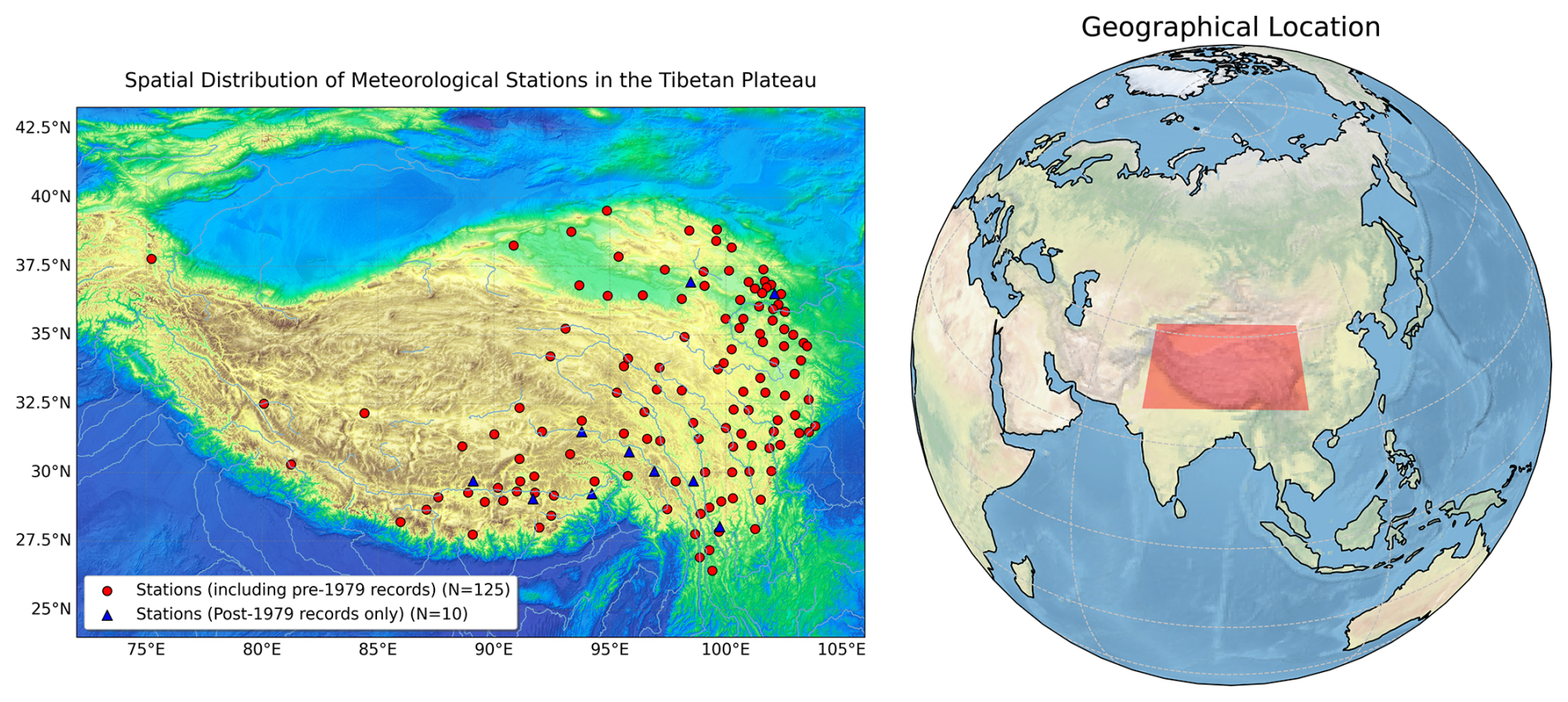
Figure 1 Geographical setting of the Tibetan Plateau. The map illustrates the complex topography and elevation gradients (left), and the study area's location within the broader Asian context (right). The 125 stations with observations extending to the pre-1979 period are shown as circles, and the 10 additional stations observed only from 1979 onward are shown as triangles, together they comprise the 135-station CMA network used for station-based consistency evaluation.

In recent years, various studies have attempted to push gridded climate data toward higher spatial resolution and longer temporal coverage (Table 1). However, except for Yang et al. (2023b), most dataset studies have relied on reference data from the 1950s onward. Moreover, current products are predominantly focused on surface air temperature and precipitation. High-resolution long-term datasets for near-surface humidity remain scarce, despite its importance for studying the TP's topographically complex land surface processes.

Table 1 Overview of recent algorithm-derived gridded products over the Tibetan Plateau.

Since the beginning of the satellite observation era (1980s to present), regional high-resolution gridded datasets, such as the Tibetan Plateau Multi-source Meteorological Forcing Dataset (TPMFD; Jiang et al., 2025), developed through machine learning and multi-source data fusion, provides the high-resolution target fields for model training and target-referenced performance assessment. By contrast, the Climatic Research Unit gridded Time Series v4.08 (CRU TS v4.08; Harris et al., 2020), utilizing the climate anomaly method and angular-distance weighting, provides continuous monthly coverage extending back to 1901. Establishing an efficient spatial downscaling framework to map these centennial-scale CRU signals onto high-resolution grids (Fig. 2), such as the TPMFD, would enable the reconstruction of a long-term, high-resolution climate record for the TP.

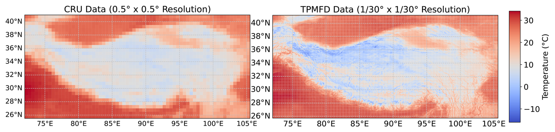
Figure 2 Visual comparison of spatial resolution between the predictor dataset and the target dataset. Left: Coarse-resolution CRU_TS_4.08 (0.5° × 0.5°). Right: High-resolution TPMFD target ($\mathrm{1}/\mathrm{30}$° × $\mathrm{1}/\mathrm{30}$°). The contrast highlights the necessity for super-resolution reconstruction to capture local topographic climate details.

Bridging the gap between long-term coarse historical data and short-term high-resolution modern instrument data has long been a challenge, and is often dealt with by downscaling. Dynamical downscaling (e.g., RCM WRF) (Prein et al., 2015) has the advantage of physical consistency but is not now feasible to be used in centennial-scale simulations at convection-permitting (e.g., at 3 km × 3 km) resolution due to extremely high computational demand. Meanwhile, Deep Learning (DL) has recently become a popular and effective alternative for statistical downscaling (Vandal et al., 2017) and climate reconstruction. DL models differ from conventional statistical approaches in that they are able to represent intricate, non-linear spatial relationships in large-scale atmospheric fields non-linearly. In this sense, FourCastNet (Pathak et al., 2022), a recently proposed global weather forecasting model exploiting the Transformer architecture developed by NVIDIA^®, has several distinctive characteristics. Its architecture is based on the composition of Vision Transformers (ViT) Dosovitskiy (2020) and Adaptive Fourier Neural Operators (AFNO) Guibas et al. (2021), to efficiently capture not only local land surface process but also global atmospheric circulation patterns. Although FourCastNet was originally designed for forecasting, its ability to learn multiscale spatial dependencies can be adapted to statistical downscaling.

Two considerations motivate the downscaling design. First, temperature, humidity, and pressure over the Tibetan Plateau exhibit persistent terrain-related spatial gradients. Second, the AFNO–ViT architecture can learn multiscale statistical mappings between coarse CRU_TS predictors and high-resolution TPMFD target fields. The resulting fine-scale patterns are interpreted as learned terrain-related relationships; the architecture and loss function do not explicitly enforce thermodynamic equations, conservation laws, or dynamical constraints.

Therefore, we leverage the FourCastNet model to reconstruct the historical high-resolution climate fields over the TP. We utilize the long-term consistency of CRU_TS_4.08 (1901–2023) as the predictor and the high spatial resolution of TPMFD ($\mathrm{1}/\mathrm{30}$° × $\mathrm{1}/\mathrm{30}$°, 1979–2023) as the target dataset. By adapting the FourCastNet framework to learn the mapping between coarse-resolution historical patterns and fine-scale topographic climate features, we produced the TPHH (Tibetan Plateau Historical High) dataset. This dataset provides reconstructed monthly 2 m temperature, 2 m specific humidity, and surface pressure at $\mathrm{1}/\mathrm{30}$° × $\mathrm{1}/\mathrm{30}$° resolution for 1901–2023. Comparisons with gridded products and station-based consistency evaluations indicate that TPHH reproduces several large-scale and station-observed statistical features. Because CMA observations may overlap indirectly with information used in TPMFD production, these comparisons are not treated as fully independent validation.

2 Data

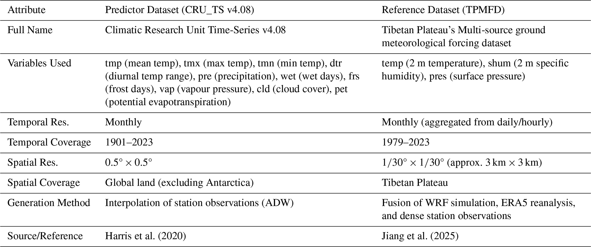
The reconstruction framework in this study is based on two datasets: CRU serving as the predictors and TPMFD as the high-resolution target dataset. The key attributes of these two datasets are detailed in the table below (Table 2).

Table 2 Overview of the predictor and reference datasets.

2.1 Climatic Research Unit Time-Series

The variables used in this study were sourced from the CRU_TS_4.08 dataset (Harris et al., 2020), a widely used global gridded climate dataset produced by the Climatic Research Unit (CRU) at the University of East Anglia. The generation process for this dataset is both complex and rigorous, with its foundation being the monthly observations from thousands of meteorological stations worldwide. Its core construction methodology is analogous to an “anomaly” or “delta” method, involving the following steps:

1. Calculation of station anomalies: Initially, observational series from over 5000 weather stations globally are utilized. The monthly observational data from each station is converted into an anomaly series by comparing it against the station's monthly mean for the 1961–1990 standard period. Anomalies for temperature-based variables are calculated by subtraction, while precipitation anomalies are calculated by division.

2. Spatial interpolation: Then, the anomaly time series of all stations are interpolated on a 0.5° × 0.5° (30 arcmin) grid over the global land surface.

3. Reconstitution of absolute values: Finally, these gridded anomaly results are merged with an independent, high-resolution 1961–1990 reference climatology product. This process converts the anomalies to absolute values of climate. Notably, the reference climatology dataset used for reconstitution itself accounts for the effects of geographical latitude, longitude, and elevation. The elevation data it incorporates is a 30 arcmin resolution Digital Elevation Model (DEM), which was derived by averaging a finer 5 arcmin global DEM. It is through this mechanism that the CRU dataset can effectively represent the influence of topography and orographic effects on the spatial distribution of climate variables at its 0.5° × 0.5° resolution. The dataset has a temporal span from January 1901 to December 2023. In this work, all 10 variables were considered as input features to the model: mean near-surface air temperature (tmp), maximum air temperature (tmx), minimum air temperature (tmn), diurnal temperature range (dtr), precipitation (pre), wet-day frequency (wet), frost-day frequency (frs), vapor pressure (vap), cloud cover (cld), and potential evapotranspiration (pet).

2.2 Tibetan Plateau Multi-source ground meteorological forcing dataset

The TPMFD dataset was used as the target dataset for model training and target-referenced performance assessment. It is a high-resolution ground meteorological forcing dataset developed specifically for the Tibetan Plateau, with a temporal coverage from 1979–2023 and a spatial resolution as high as $\mathrm{1}/\mathrm{30}$°. Its high spatial resolution is produced through multi-source fusion: 2 m temperature, 2 m specific humidity, surface pressure, and wind speed are derived from the fusion of short-term high-resolution WRF simulations, long-term ERA5 data, and dense ground station observations (Jiang et al., 2025). This fusion combines dynamical-model output, reanalysis fields, and station-based corrections, while retaining uncertainties inherited from each source. TPMFD is therefore used as the high-resolution target dataset rather than as error-free ground truth. We use its 2 m temperature (temp), 2 m specific humidity (shum), and surface pressure (pres) fields for 1979–2023. TPMFD is described and accessed through Jiang et al. (2025) and its corresponding repository: https://doi.org/10.11888/atmos.tpdc.300398 (Yang et al., 2023a).

2.3 Site observations

For station-based consistency evaluation, we compiled monthly 2 m temperature, surface pressure, and relative-humidity records from 135 China Meteorological Administration (CMA) stations. The temperature and relative-humidity series were quality controlled and homogenized following Cao et al. (2016) and Zhu et al. (2015), respectively. Because CMA observations contributed to TPMFD production, possible information overlap cannot be excluded. The spatial distribution of the collected sites within the Tibetan Plateau is shown in Fig. 1.

Of the 135 CMA stations, 125 have observations extending to the pre-1979 period, whereas the remaining 10 have observations only from 1979 onward. For the pre-1979 records, 125 stations contained valid data, yielding 28 800 site-month records for temperature, 25 570 for pressure, 28 077 for relative humidity, and 25 422 for specific humidity. For the period of 1979–2023, 135 stations provided 68 840 records for temperature, 70 411 for pressure, 68 714 for relative humidity, and 68 661 for specific humidity.

2.4 Comparable datasets

To compare selected statistical characteristics of TPHH with existing products, we considered reanalysis datasets, gridded observations, and climate-model simulations.

In addition to ERA5-Land (1950–present) (Muñoz-Sabater et al., 2021) and 20CRv3 (1836–2015) (Slivinski et al., 2019), we included two widely used reanalysis datasets: the Japanese Reanalysis for Three Quarters of a Century (JRA-3Q, 1948–present) (Harada et al., 2026) and the NCEP/NCAR Reanalysis 1 (NCEP-R1, 1948–present) (Kalnay et al., 1996). For gridded observations, we utilized the UDel (University of Delaware) air temperature and precipitation dataset (V5.01, 1900–2017) (Willmott, 2000). For downscaling-based reconstructions, we utilized the 1 km monthly temperature (1901–2024) developed by Peng et al. (2019). Furthermore, to assess the model's performance against traditional climate models, we selected historical simulations (covering 1850–2014) from six GCMs participating in the Coupled Model Intercomparison Project Phase 6 (CMIP6) (O'Neill et al., 2016): CESM2, UKESM1-0-LL, MPI-ESMI-2-HR, IPSL-CM6A-LR, BCC-CSM2-MR, and CanESM5. All CMIP6 data were bilinearly interpolated to the target resolution for consistent comparison.

3 Methodology

3.1 Hybrid-structure Downscaling Model: FourCastNet

An efficient downscaling model is key to bridging the resolution gap. In this study, we employ FourCastNet as the core downscaling model for handling the complex spatiotemporal physical fields over the TP. As a data-driven weather model, FourCastNet is one of the state-of-the-art deep learning models originally designed for global machine-learning-based weather forecasting. Its architecture combines the strengths of computer vision and Fourier neural operators, making it particularly suitable for the climate data downscaling task in our study. Its core advantage lies in its ability to efficiently learn multi-scale spatial features and total-field dependencies, which is crucial for downscaling climate fields from coarse CRU gridded data over the complex terrain of the TP. The production configuration, software, and hardware details are provided in Table S1 in the Supplement.

The hybrid-structure of the model is primarily composed of two key components: a Vision Transformer (ViT) backbone and the Adaptive Fourier Neural Operator (AFNO) serving as the core mixing layer.

3.1.1 Vision Transformer (ViT) Backbone

FourCastNet leverages successes from the field of computer vision, treating the input two-dimensional multi-channel climate field (where each channel represents a CRU variable like temperature, precipitation, etc.) as an “image”. The ViT backbone first divides this “image” into a series of non-overlapping, fixed-size patches. Each patch is then linearly projected into a one-dimensional vector. This approach offers two main advantages:

1. Dimensionality reduction and efficiency: By aggregating pixels into patches, the model significantly reduces the spatial resolution of the input data, transforming high-dimensional climate fields into a manageable sequence of tokens. This lowers the computational complexity, making it feasible to process high-resolution data.

2. Global context modeling: Transforming the 2D grid into a sequence of tokens allows the subsequent Transformer architecture to effectively capture long-range dependencies between distant patches, rather than being limited to local receptive fields.

3.1.2 Core Mixing Layer: Adaptive Fourier Neural Operator (AFNO)

In a standard ViT model, the mechanism for mixing information between different patches is multi-head self-attention. However, its computational complexity grows quadratically with the number of patches, making it computationally expensive for high-resolution climate data.

The core innovation of FourCastNet is the use of AFNO as a replacement mixing layer. The principle of AFNO is based on the Fourier Neural Operator (FNO) (Li et al., 2023), which performs computations in the Fourier domain to capture global information with remarkable efficiency. The basic process is as follows:

1. Fourier transform: Initially the information in the spatial domain, i.e., the sequence of patches, is converted to the frequency domain via a Fast Fourier Transform (FFT).

2. Frequency-domain learning: The model, in the frequency domain, learns the correlations of different frequency modes by channel mixing. Additionally, comparing to the local receptive fields in Convolutional Neural Networks (CNNs), the basic functions for the Fourier transform (sine and cosine waves) are global. Hence, an operation in the frequency domain inherently has a global spatial processing.

3. Inverse Fourier transform: At last, the learned and modified frequency domain representation is mapped back to the spatial domain by an Inverse Fast Fourier Transform (IFFT).

The “Adaptive” characteristic of AFNO is an improvement upon FNO. It introduces a soft-thresholding and sparsity mechanism, which allows the model to adaptively filter and retain the frequency information that is most important for the reconstruction task, rather than simply truncating high-frequency signals as in the original FNO. This makes AFNO more computationally efficient and powerful.

3.1.3 Model Application in This Study

Within the framework of this study, FourCastNet operates as follows:

1. Input: A 3D tensor with dimensions input variables × latitude × longitude, interpreted as a multi-channel 2D spatial grid field. Each channel represents a climate variable, for instance temperature, vapor pressure, or cloud cover, from the CRU dataset.

2. Processing: Prior to patch embedding, the coarse CRU input is spatially interpolated to match the high-resolution target grid. The upsampled CRU data is then patched by the ViT backbone and processed through multiple stacked layers of AFNO mixers. The model learns the complex nonlinear statistical relationships between the upsampled CRU_TS predictors and TPMFD target fields in both the frequency and spatial domains.

3. Output: A multi-channel 2D array with the same high spatial resolution as TPMFD ($\mathrm{1}/\mathrm{30}$° × $\mathrm{1}/\mathrm{30}$°). Each output channel corresponds to a target variable we aim to reconstruct (2 m temperature, 2 m specific humidity, surface pressure).

3.1.4 Assembly of the production reconstruction

The model outputs were assembled differently for the overlap and historical periods. For 1979–2023, the 45-year period was divided into nine mutually exclusive five-year test blocks. Each block was reconstructed using the corresponding fold model for which that block had been excluded from training. The nine non-overlapping out-of-fold predictions were then concatenated chronologically, so that each monthly time step during 1979–2023 was represented once in the final reconstruction. For 1901–1978, all nine trained fold models were applied to the historical CRU_TS predictors, and the arithmetic mean of their nine predictions was used as the final historical reconstruction.

3.2 Reconstruction Workflow

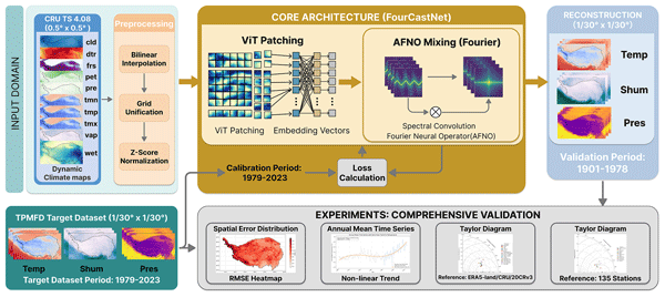
The workflow of our approach is visually displayed in Fig. 3, showing the overall workflow from data preprocessing to final evaluation. As shown in Fig. 3, the reconstruction pipeline is composed of four successive steps:

1. Domain of input and optimization: The information used is dynamic climate maps from CRU. Next, following a bilinear interpolation, the coarse climate fields are concatenated to form the multi-channel input tensor for the deep learning model.

2. Core architecture (FourCastNet): The refined features are input into the FourCastNet model. The ViT patch-embedding module converts the grid into patch tokens, after which AFNO mixers use fast Fourier transforms and spectral operations to exchange information efficiently in the frequency domain.

3. Training and loss computation: The model was trained to map the upsampled CRU_TS predictors to the high-resolution TPMFD target fields for 1979–2023 by minimizing mean squared error.

4. Outputs for 1979–2023 were evaluated against TPMFD through nine-fold target-referenced cross-validation. Historical temporal behavior was assessed using station-based consistency comparisons, multi-product comparisons, Pettitt breakpoint tests, monthly trend diagnostics, and tree-ring proxy-window analyses. The CMA comparisons are not treated as independent because information overlap with TPMFD cannot be excluded.

Below are more detailed descriptions for the individual steps.

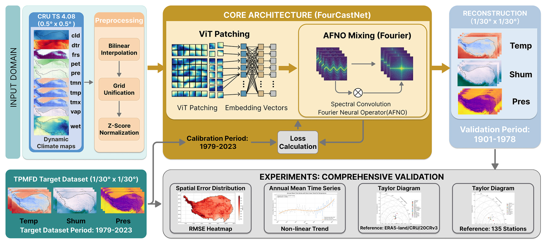
Figure 3 Schematic diagram of the methodology to generate the TPHH. The pipeline begins at the input domain with coarse climate fields. Major components are (1) Input processing, where coarse climate variables are prepared and embedded, (2) The main FourCastNet architecture, based on a ViT (Vision Transformer) backbone for patching and an AFNO (Adaptive Fourier Neural Operator) as local-global information mixing operator in the frequency domain, (3) Training with TPMFD dataset (1979–2023) through loss computation; and (4) Evaluation, comprising target-referenced performance assessment for 1979–2023 and station-based, breakpoint, trend, DEM-sensitivity, and proxy-window diagnostics.

3.2.1 Data Pre-processing

1. Spatial interpolation: For the spatial resolutions of the predictor and predictand data to be consistent, the original 0.5° CRU_TS fields were bilinearly upsampled to the $\mathrm{1}/\mathrm{30}$° TPMFD grid.

2. Data normalization: To avoid the effect of differing scales of variables and make the model converge faster, we normalized all the input data. In particular, within each fold and for each grid cell and calendar month, normalization means and standard deviations were calculated from the training years only and then applied to the held-out years. Each value was standardized by subtracting the corresponding training mean and dividing by the corresponding training standard deviation. Then, each value on that grid was normalized by subtracting the mean and dividing by the standard deviation. Such per-grid-cell normalization is important to ensure that the local climatology for each point is preserved while training.

3.2.2 Model Calibration

1. Calibration period: We took advantage of the intersection period of the two data sources, 1979–2023 for the model training and cross-validation (45 years in total).

2. Cross-validation: To exploit data to its best and to get a reliable assessment of performance, we used nine-fold cross-validation. The 45-year overlap period (1979–2023) was divided into nine non-overlapping five-year test blocks; in each iteration, 40 years were used for training and the remaining five-year block for testing. Fold-level metrics and their arithmetic means are reported in Tables S2 and 3, respectively.

3.2.3 Historical Validation

Upon completion of the training and validation phase, the nine-fold-specific models were retained as an ensemble for production inference. The CRU data for the period 1901–1978 were pre-processed using the same normalization parameters derived from the 1979–2023 period. This historical data was then fed into the trained model to generate the high-resolution ($\mathrm{1}/\mathrm{30}$° × $\mathrm{1}/\mathrm{30}$°), monthly reconstructions of 2 m temperature, 2 m specific humidity, and surface pressure.

3.3 Accuracy Metrics

To evaluate the quality of the reconstruction model quantitatively, we compared reconstructed fields with the TPMFD target fields during 1979–2023 using a suite of common statistical metrics, namely coefficient of determination (R²), Root Mean Square Error (RMSE), Mean Absolute Error (MAE) and the Index of Agreement (IOA).

In the following equations, S_i denotes the simulated value at time step i, O_i denotes the target TPMFD value, and $\stackrel{\mathrm{‾}}{S}$ and $\stackrel{\mathrm{‾}}{O}$ denote the mean of the simulated and target values, respectively. The number of all samples is n.

1. Coefficient of determination (R²): This measure indicates how much variance in the observed data can be accounted for by the model. It shows how strongly linear simulated and targeted values are related. Larger values of R² indicate better model fits. Its value lies between 0 and 1, and 1 denotes a perfect correlation.

   $$\begin{array}{}\text{(1)}& R^{\mathrm{2}}={\left({\displaystyle \frac{\sum _{i=\mathrm{1}}^n(S_i-\stackrel{\mathrm{‾}}{S})(O_i-\stackrel{\mathrm{‾}}{O})}{\sqrt{\sum _{i=\mathrm{1}}^n(S_i-\stackrel{\mathrm{‾}}{S}{)}^{\mathrm{2}}}\sqrt{\sum _{i=\mathrm{1}}^n(O_i-\stackrel{\mathrm{‾}}{O}{)}^{\mathrm{2}}}}}\right)}^{\mathrm{2}}\end{array}$$

2. Root Mean Square Error (RMSE): RMSE is the square root of the mean squared difference between reconstructed and TPMFD target values. It can be interpreted as the average size of the error in the same units as the predicted variable. Smaller RMSE is better, and it means a more accurate model prediction. The best value is 0.

   $$\begin{array}{}\text{(2)}& \mathrm{RMSE}=\sqrt{{\displaystyle \frac{\mathrm{1}}{n}}\sum _{i=\mathrm{1}}^n(S_i-O_i{)}^{\mathrm{2}}}\end{array}$$

3. Mean Absolute Error (MAE): The MAE measures the average size of the errors in a set of forecasts, without considering their direction. In contrast to Mean Bias, it does not take into account the sign of the error (i.e., whether the prediction is too high or too low). It gives a clean and unambiguous indication of how large, on average, the errors are. A smaller MAE value indicates the better performance of the model with the best value of 0.

   $$\begin{array}{}\text{(3)}& \mathrm{MAE}={\displaystyle \frac{\mathrm{1}}{n}}\sum _{i=\mathrm{1}}^n|S_i-O_i|\end{array}$$

4. Index of Agreement (IOA): The IOA is a standardized measure of the degree of model prediction error. It is more sensitive to differences in the targeted and simulated means and variances than the R² value. The IOA ranges from 0 to 1, where 1 indicates perfect agreement between the model and the observations, and 0 indicates no agreement.

   $$\begin{array}{}\text{(4)}& \mathrm{IOA}=\mathrm{1}-{\displaystyle \frac{\sum _{i=\mathrm{1}}^n(S_i-O_i{)}^{\mathrm{2}}}{\sum _{i=\mathrm{1}}^n\left(\right|S_i-\stackrel{\mathrm{‾}}{O}|+|O_i-\stackrel{\mathrm{‾}}{O}|{)}^{\mathrm{2}}}}\end{array}$$

3.4 Spatial, Temporal, and Statistical Evaluation of the Reconstructed Dataset

In addition to the primary accuracy metrics, a series of graphical and comparative analyses were conducted to provide complementary reconstruction-performance, station-consistency, breakpoint, trend, DEM-sensitivity, and proxy-window diagnostics. These diagnostics assess different aspects of consistency and plausibility but do not constitute a comprehensive uncertainty estimate. The roles and limitations of each diagnostic are described below.

1. Density scatter plots: To evaluate the validity of point-to-point matching and error distribution (1979–2023) for 2 m temperature (temp), 2 m specific humidity (shum), and surface pressure (pres), density scatter plots were used. The first shows the predictions of the nine individual models produced by nine-fold cross-validation against the corresponding TPMFD target values. The plots reveal systematic departures, scatter, and the concentration of samples around the 1 : 1 line.

2. Temporal behavior was evaluated using Plateau-mean and station-network-mean series, grid-cell Pettitt breakpoint tests, and monthly linear-trend diagnostics for 1901–1930, 1931–1960, 1961–1990, 1991–2020, and 1994–2023. These analyses diagnose stability and plausibility, to assess breakpoint prevalence and period-specific trend behavior without treating these diagnostics as direct estimates of pre-1950 error.

3. Full-domain R², RMSE, MAE, and IOA maps were calculated against TPMFD for 1979–2008 and 1994–2023. The same metrics were also compared between otherwise identical models trained with and without an explicit DEM channel (Figs. S24–S29 in the Supplement). These maps are target-referenced performance diagnostics rather than uncertainty maps for unmonitored regions.

4. Taylor diagrams for inter-comparison: To offer a concise statistical summary of model performance, Taylor diagrams were employed. This analysis was performed in two distinct ways. First, a Taylor diagram was constructed using the CMA station observations for station-based consistency evaluation. Up to 125 stations contributed observations in the pre-1979 period, and up to 135 were available after 1979, and possible information overlap with TPMFD precludes treating these records as independent validation. The diagrams therefore provide station-based consistency assessments.

Second, to place our model's performance in the context of other widely-used climate datasets, a series of Taylor diagrams were produced using multiple gridded data products as references. These comparisons describe how TPHH reproduces selected statistical properties relative to different products. Agreement among products is interpreted as inter-product consistency rather than independent validation. The specific comparisons were as follows: temp was compared against 20CRv3, ERA5, and CRU_TS_4.08; shum was compared against 20CRv3 and ERA5; pres was compared against 20CRv3 and ERA5.

3.5 Proxy-based temporal-plausibility evaluation using tree-ring data

To examine proxy-based temporal plausibility, we fitted a standardized ternary regression model to 41 tree-ring chronology groups. The model combined JJA temperature, a candidate moisture window (AMJ, MJJ, or JJA specific humidity), and a lag-1 tree-ring term. Prior to modeling, the TPHH summer temperature (T_JJA), the early-summer specific humidity (Q_MJJ), and the tree-ring width index (TRWI) (Fang et al., 2022), were standardized using Z-score normalization to eliminate dimensional discrepancies. To represent contemporaneous climatic covariates together with serial persistence in the tree-ring chronology, the current-year thermal and moisture variables were combined with a first-order autoregressive term (the lag-1 TRWI_t−1). The normalized ternary model is expressed as:

$$\begin{array}{}\text{(5)}& {\mathrm{TRWI}}_t={\mathit{\beta }}_{\mathrm{0}}+{\mathit{\beta }}_{\mathrm{1}}\times T_{\mathrm{JJA}}+{\mathit{\beta }}_{\mathrm{2}}\times Q_{\mathrm{MJJ}}+{\mathit{\beta }}_{\mathrm{3}}\times {\mathrm{TRWI}}_{t-\mathrm{1}}\end{array}$$

This standardized modeling effectively estimates the interannual theoretical tree growth driven by the TPHH historical climate. An 11-year moving average was shown only to visualize low-frequency co-variation.

4 Results

4.1 Model performance cross-validation

To assess the ability of the hybrid-structure deep-learning model (FourCastNet) to reconstruct high-resolution climate fields from CRU predictors, we performed a target-referenced performance assessment of its output using the TPMFD dataset during 1979–2023 as the target dataset.

4.1.1 Overall Quantitative Metrics

For each variable, R², RMSE, MAE, and IOA were calculated separately for each of the nine held-out folds. Table 3 reports the arithmetic means of the nine-fold-level values, while Table S2 reports the individual fold values. The released Table S2 preserves the same fold-level statistical basis.

Table 3 Arithmetic-mean performance metrics from nine-fold cross-validation during 1979–2023, evaluated against the TPMFD target fields.

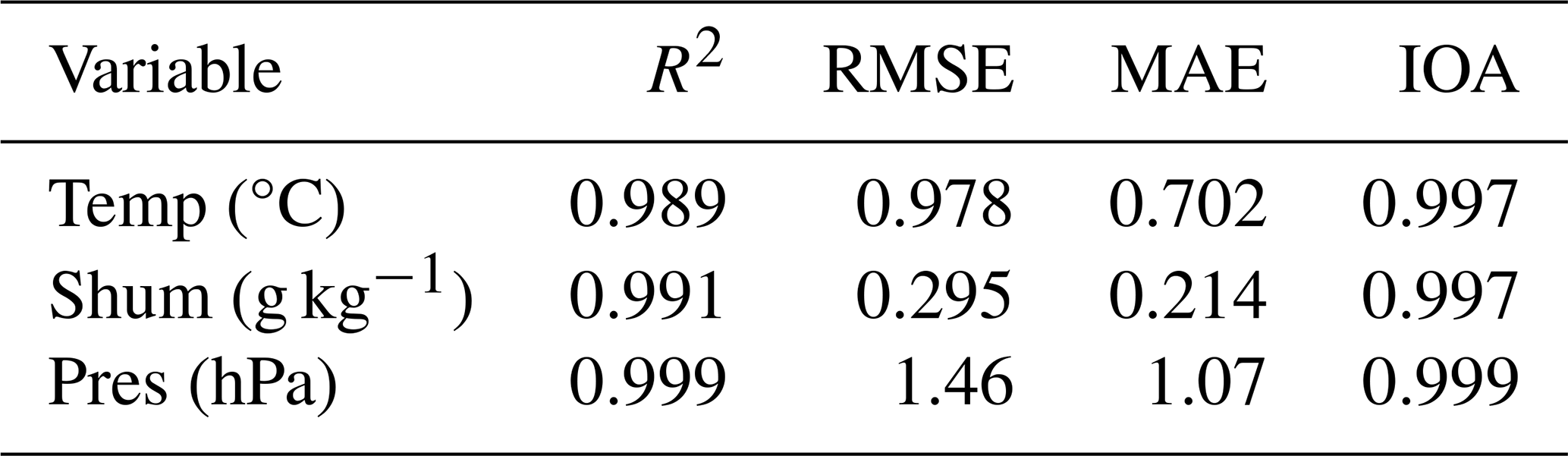
The nine-fold means in Table 3 indicate strong agreement with TPMFD during 1979–2023. Mean R² values were 0.989, 0.991, and 0.999 for temperature, specific humidity, and pressure, respectively, and the corresponding RMSE values were 0.978 °C, 0.295 g kg⁻¹, and 1.46 hPa. These target-referenced metrics quantify reconstruction performance of TPHH during 1979–2023.

4.1.2 Consistency between reconstructed and TPMFD target values

To more intuitively assess the consistency between the model's predictions and the TPMFD reference data, we generated density scatter plots (2D histograms). This analysis aggregates all data points from the test sets of the nine-fold cross-validation. The aggregated test sets comprised 540 monthly time steps spanning the 45-year period.

Firstly, for each variable, we calculated the “overall validation plots” (Fig. 4), which include all data points of all months. It can be seen that the data for temp, shum and pres are tightly clustered around the 1 : 1 diagonal line. The concentration around the 1 : 1 line indicates close overall agreement with TPMFD, while systematic bias should be assessed using explicit bias statistics rather than inferred solely from visual density.

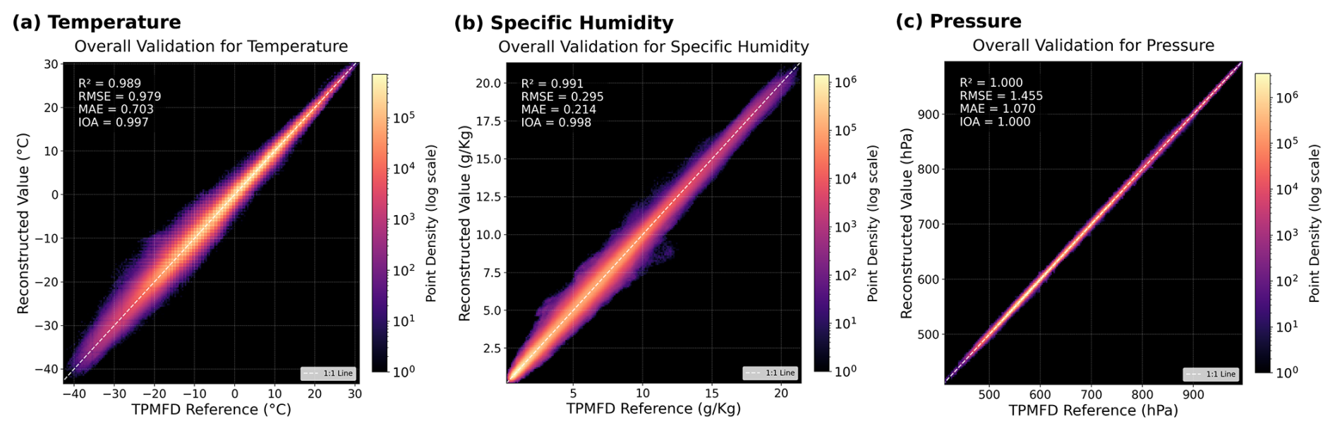
Figure 4 Overall density scatter plots for (a) temp, (b) shum, and (c) pres based on all 540 test time steps from the nine-fold cross-validation (1979–2023). Colors indicate point density on a logarithmic scale.

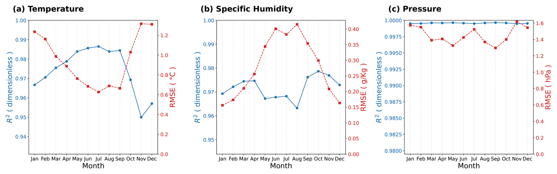
Figure 5 Seasonal cycle of model performance (1979–2023). Each panel shows the selected metrics (R² and RMSE) calculated for each month of the year, based on the nine-fold validation results for (a) temp, (b) shum, and (c) pres.

Next, to investigate potential seasonal variations in model fidelity, we analyzed the performance metrics for each of the 12 months. A full set of 36 monthly density scatter plots is provided in the Supplement (Figs. S1–S3). To summarize the seasonal cycle of model performance, we plot the monthly-stratified metrics in Fig. 5.

This examination makes apparent the regular seasonality. Temperature RMSE was larger in winter, whereas specific-humidity RMSE increased during several monsoon-season months. These seasonal differences are descriptive; their physical causes were not directly tested. R² remained above 0.95 across calendar months, indicating consistently high target-referenced agreement during 1979–2023.

4.1.3 Spatial distribution of model performance

To investigate the spatial variations in model performance, we mapped the spatial distribution of performance metrics for the study region. This analysis is also based on all 540 months serving as time steps from the nine-fold cross-validation. The results for all 12 metric-variable combinations are compiled in Fig. 6.

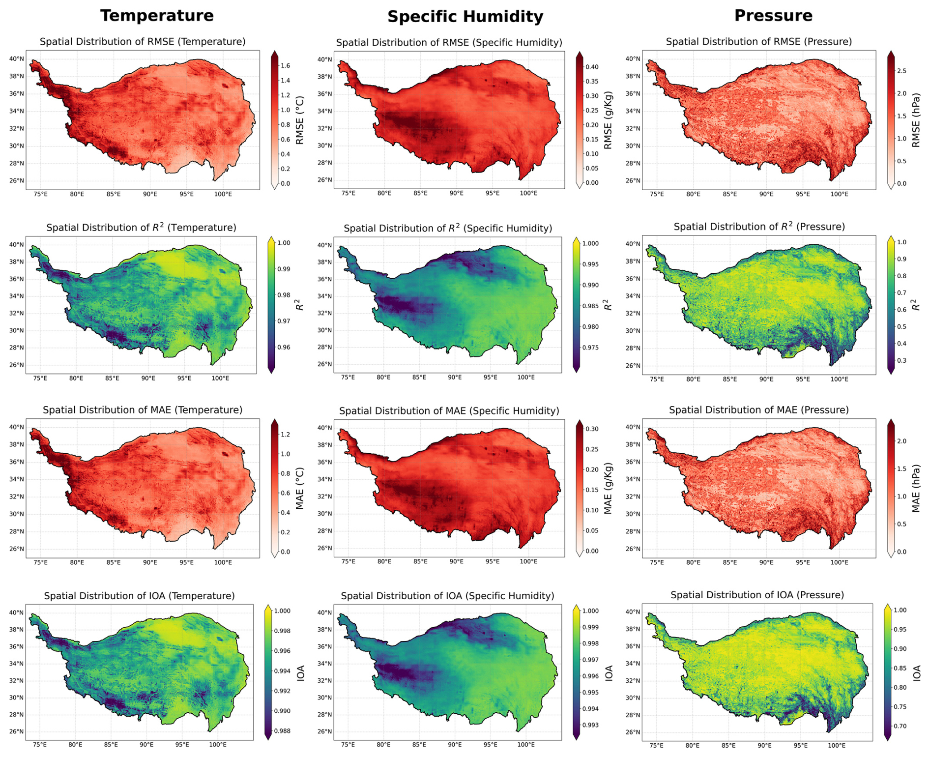
Figure 6 Spatial patterns of metrics (1979–2023). The matrix contains the performance metrics in the rows and the variables in the columns: Rows: (1) RMSE, (2) R², (3) MAE, and (4) IOA. Columns: (Left) surface temperature, (Middle) specific humidity, and (Right) surface pressure.

Figure 6 demonstrates spatial variations of model performance. In general, the model is more accurate over the central interior basins and the more level portions of the TP. This is shown by consistently high R² and IOA (second and fourth rows) and low error values (first and third rows).

Larger target-referenced RMSE and MAE occur near steep terrain transitions, including the southern Himalaya and Hengduan Mountains. Pressure metrics are spatially more uniform than the temperature and humidity metrics. Because the model did not explicitly ingest elevation in the production configuration, these patterns are interpreted as learned statistical relationships rather than proof that terrain was explicitly or physically constrained.

4.2 Evaluation of the reconstruction

Having demonstrated the model's calibration performance, we now turn to performance validation of reconstruction. We employed two complementary comparison strategies: (1) station-based consistency evaluation using CMA records, and (2) inter-product statistical comparison. Neither strategy is interpreted as fully independent validation of early-period accuracy.

4.2.1 Site-observation-based consistency evaluation

We evaluated station-based consistency using a total CMA network of 135 stations, of which 125 have observations extending to the pre-1979 period and 10 additional stations have observations only from 1979 onward. Gridded values were interpolated to station locations and compared with simultaneous station records. Because CMA information may have contributed to TPMFD, these comparisons are not treated as independent. The nine-fold model cross-validation against TPMFD is described separately in Sect. 3.2.2.

Figure 7 summarizes the relative standard deviations and correlations of TPHH and selected products with the available CMA station records. The comparison indicates station-based consistency but may be influenced by shared observational information:

1. For Surface air temperature (Fig. 7a, d), most products have standard deviations between 8–10 (°C), close to the station-reference standard deviation of ∼ 9 °C. The main strength of TPHH is its high correlation coefficient. All products exhibited nearly unchanged relative diagram positions in the two periods before and after 1979.

2. In the case of specific humidity (Fig. 7b, e), the ERA, JRA, 20CR products all have substantially smaller standard deviations than site-observations, while the other products have closer standard deviation but lower correlation coefficients. Within the products and station samples, TPHH had the closest combination of relative standard deviation and correlation for specific humidity.

3. For surface pressure (Fig. 7c, f), TPHH showed the highest correlation among the products included in this station-based comparison.

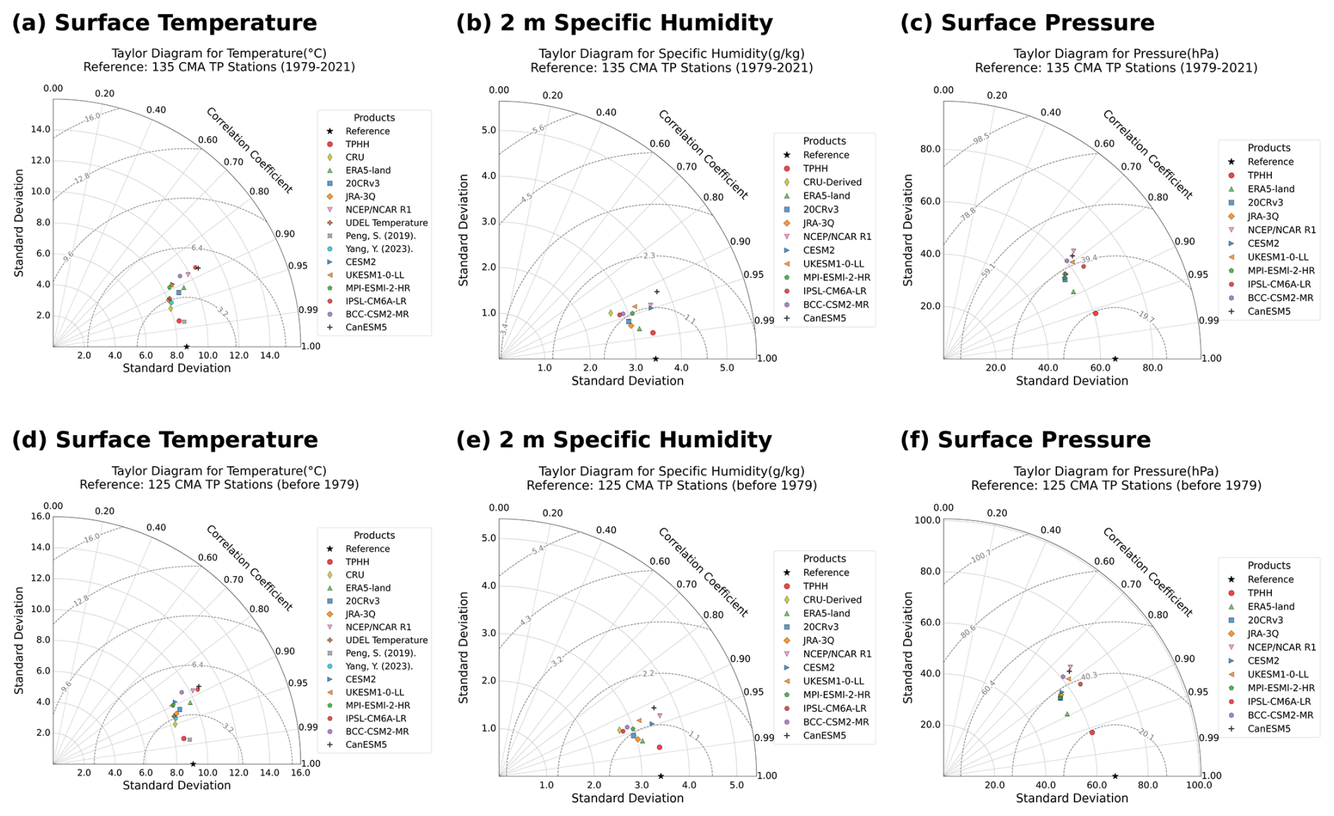
Figure 7 Taylor diagrams comparing our reconstruction (TPHH, red circle) and other climate products against CMA site observations. The top row (a–c) evaluates the calibration period (1979–2021) based on 135 stations, and the bottom row (d–f) evaluates the historical station-based consistency within pre-1979 based on 125 stations for surface temperature, 2 m specific humidity, and surface pressure, respectively. The reference point (black star) represents in-situ site observations.

These results show close statistical agreement with available station records during the evaluated periods. Although they do not demonstrate station independence or uniform reliability over the western and central high-elevation Plateau, where observations remain sparse, they could support the credibility of TPHH in terms of temporal and multiple-product-metric stability.

4.2.2 Inter-comparison with comparable products

To further assess the statistical plausibility (e.g., spatial variability, correlation) of the reconstructed data, we conducted a broader comparison of TPHH against more than ten related products. We performed seven Taylor diagram analyses, each using a different dataset (e.g., ERA5-Land, JRA-3Q) as the benchmarking reference.

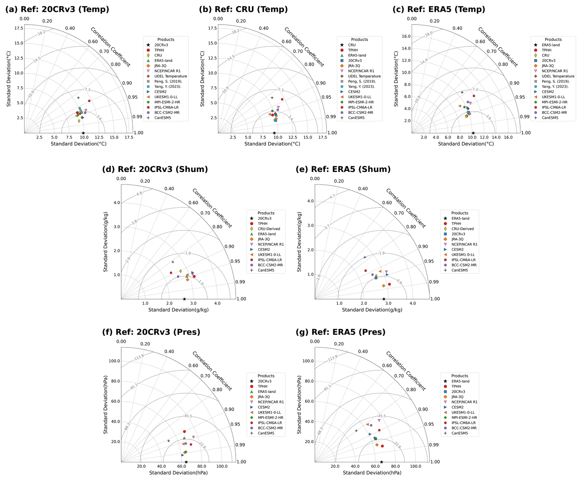
Figure 8 Taylor diagrams for multi-product inter-comparison (before 1979). (a–c) Top row: temperature (temp, units: °C) comparison against (a) 20CRv3, (b) CRU, and (c) ERA5. (d–e) Middle row: specific humidity (shum, units: g kg⁻¹) comparison against (d) 20CRv3 and (e) ERA5. (f–g) Bottom row: surface pressure (pres, units: hPa) comparison against (f) 20CRv3 and (g) ERA5. The TPHH dataset is marked by a red circle.

As shown in Fig. 8, the statistical performance of TPHH varies depending on the reference benchmark, reflecting the distinct characteristics of the datasets being compared.

1. High fidelity to modern reanalysis (vs. ERA5-land). When ERA5-land (0.1° × 0.1°) is used as the reference (Fig. 8c, e, g), TPHH demonstrates remarkably high statistical similarity, clustering closely with other top-tier datasets. Specifically, only CRU and TPHH have correlation coefficients (corr.) with ERA5-land exceeding 0.95 in temperature. Besides, in case of specific humidity validation, only JRA-3Q and TPHH exceeded 0.95 with prominent advantages against other products. This confirms that, for the overlapping period where high-quality observational constraints are available, our model efficiently reproduces the synoptic-scale climatic patterns.

2. Reasonable consistency with historical baselines (vs. 20CRv3): In comparisons against the coarser 20CRv3 (1.0°), TPHH does not always occupy the position closest to the reference point (Fig. 8a, d, f). However, TPHH becomes one of the only two humidity products (another is JRA-3Q) with corr. > 0.95 again. As for the temperature, TPHH's performance level is also around the median among multiple products.

3. Fidelity to Input forcing (vs. CRU): Finally, the comparison against the predictor dataset CRU (Fig. 8b) shows an exceptionally high correlation coefficient. The high correlation with CRU_TS is expected because CRU_TS is the model predictor. This comparison shows retention of large-scale input variability but is not independent validation and cannot by itself rule out artifacts introduced during downscaling.

4.3 Analysis of spatial-temporal consistency

Having evaluated selected aspects of reconstruction performance, station consistency, and temporal plausibility, this section examines long-term spatial and temporal characteristics of TPHH.

4.3.1 Spatial patterns for long-term historical climatology (1901–1978)

To present the reconstructed historical climate baseline, we show the temporal mean over the 78-year period from 1901 to 1978, generating long-term mean spatial distribution maps for temp, shum, and pres.

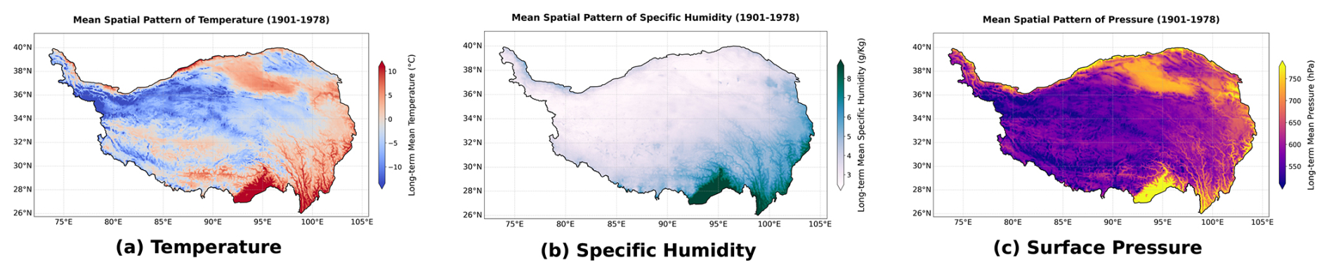
Figure 9 Long-term mean spatial distribution (1901–1978) reconstructed by TPHH. Panels show (a) surface temperature, (b) specific humidity, and (c) surface pressure. All fields are shown on the $\mathrm{1}/\mathrm{30}$° × $\mathrm{1}/\mathrm{30}$° TPHH grid and masked to the Tibetan Plateau domain.

Figure 9 presents the average climatic conditions over the Tibetan Plateau for most of the 20th century.

1. Surface air temperature (Fig. 9a): The distribution is predominantly governed by elevation and latitude, as seen in the illustration, with lower temperatures over the high-elevation northwestern Plateau and warmer conditions in the lower-elevation Qaidam Basin and southeastern valleys.

2. Specific humidity (Fig. 9b): The pattern exhibits an obvious decreasing trend from southeast to northwest. The specific-humidity field exhibits a pronounced southeast-to-northwest gradient, broadly consistent with the transport of monsoonal moisture from the Bay of Bengal into the southeastern Tibetan Plateau, for which the Yarlung Tsangpo Grand Canyon acts as a major moisture-transport passage (Yuan et al., 2023; Chen et al., 2024).

3. Surface pressure (Fig. 9c): The reconstructed pressure field shows fine-scale spatial gradients associated with the high-resolution TPMFD target patterns. Because elevation was not explicitly imposed in the production model, these structures should be interpreted as learned statistical patterns, but significantly reflected in-situ terrain.

These reconstructed $\mathrm{1}/\mathrm{30}$° climatology fields provide a spatially refined historical baseline, but early-century fine-scale patterns, especially in the western and central Plateau, remain weakly constrained by direct observations.

4.3.2 Analysis of Long-term time series continuity and trends

A key quality check is to assess the continuity at the junction between the historical reconstruction (1901–1978) and the modern reference data (1979–2023). Visual inspection of Figs. 10 and 11 was supplemented by grid-cell Pettitt tests (Figs. S30–S32). In the 1961–1990 window, 4.0 % of temperature, 2.1 % of specific-humidity, and 21.9 % of pressure grid cells had p<0.05. Significant breakpoints in 1978/1979 occurred in 1.43 %, 0.03 %, and 8.56 %, respectively. These results do not indicate a widespread transition-centered breakpoint for temperature or humidity, whereas pressure shows greater transition sensitivity. The tests assess temporal consistency rather than proving absence of artifacts or overfitting.

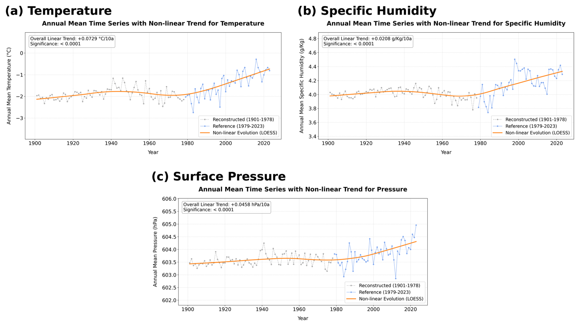
Figure 10 Annual Mean Time Series with LOESS trend for (a) temp, (b) shum, (c) pres, derived from spatial averages over the TP.

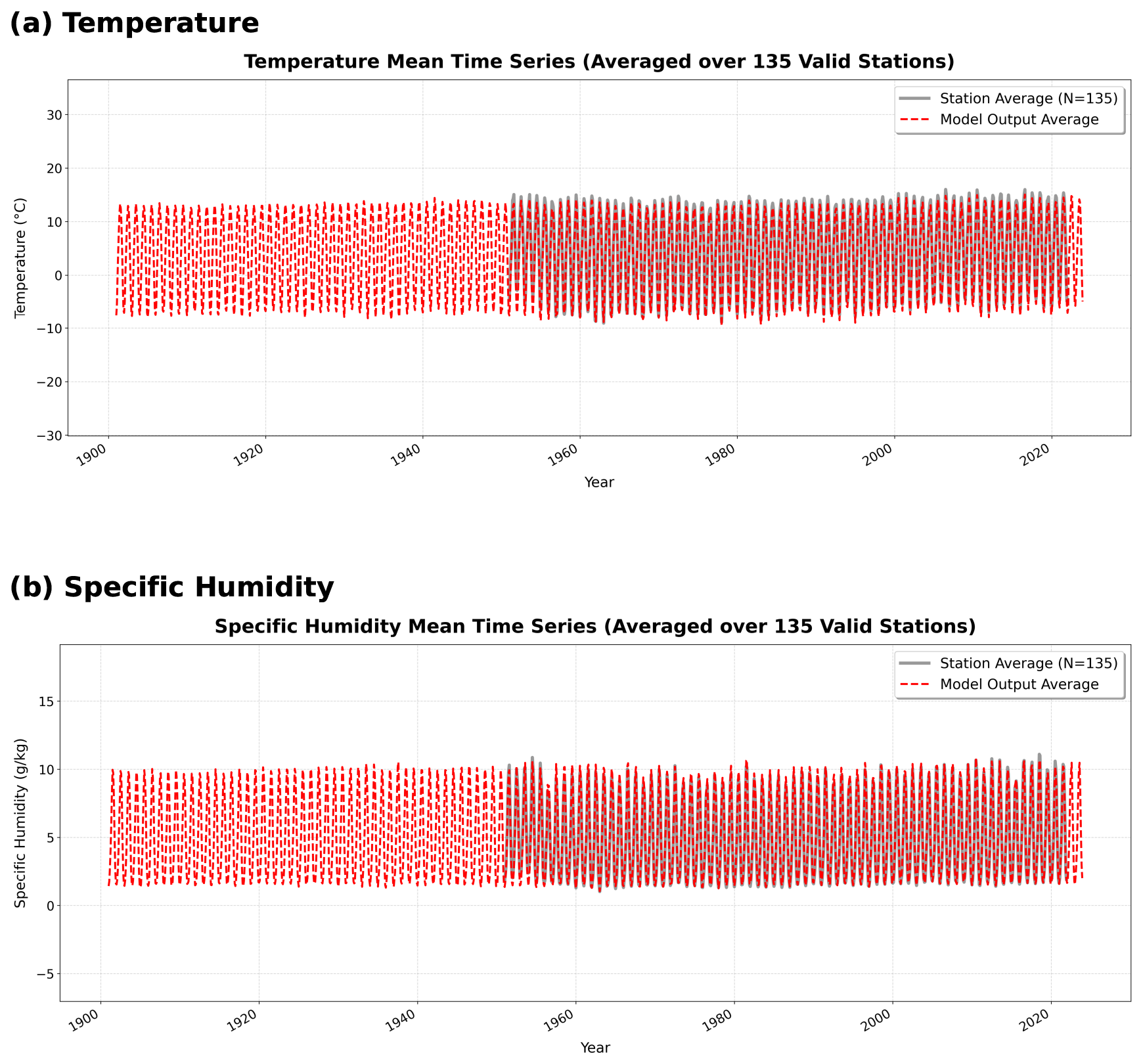
Figure 11 Time series consistency diagnosis with site-observations for temp (a) and shum (b). Shown as the averaged model output (spatial-inferred to sites) joined with the site-observation series.

Figure 10 shows Plateau-mean annual series, and Fig. 11 shows the station-network-mean consistency diagnostic. Monthly linear trends and p values were calculated for five 30-year windows and are shown in Figs. S33–S47 (temperature: Figs. S33–S37; specific humidity: Figs. S38–S42; pressure: Figs. S43–S47). These period-specific maps demonstrate spatial and temporal heterogeneity; they do not constitute a single full-period 1901–2023 trend estimate or a cross-product validation of centennial humidity change.

4.4 Proxy-based temporal-plausibility assessment using tree-ring chronologies

The fitting result demonstrates a high temporal consistency with the annual tree-ring proxy series. As illustrated in Fig. 12 for a representative chronology, the smoothed climate-driven fitted series aligns tightly with the actual proxy record, yielding a Pearson correlation coefficient exceeding 0.8. Specifically, the lag-1 autoregressive term exhibits the largest standardized coefficient (β=0.37), highlighting the dominant role of physiological inertia. This indicates that radial growth on the TP is heavily subsidized by non-structural carbohydrates stored in the preceding year. Early-summer specific humidity emerges as the primary limiting factor (β=0.26), with a contribution nearly three times greater than that of peak growing-season temperature (β=0.05). This long-term coherence confirms that the TPHH dataset captures a part of the annual climate fluctuations. The spatial distribution and fitting results for totally 41 groups of proxy locations are detailed in Figs. S8–S23.

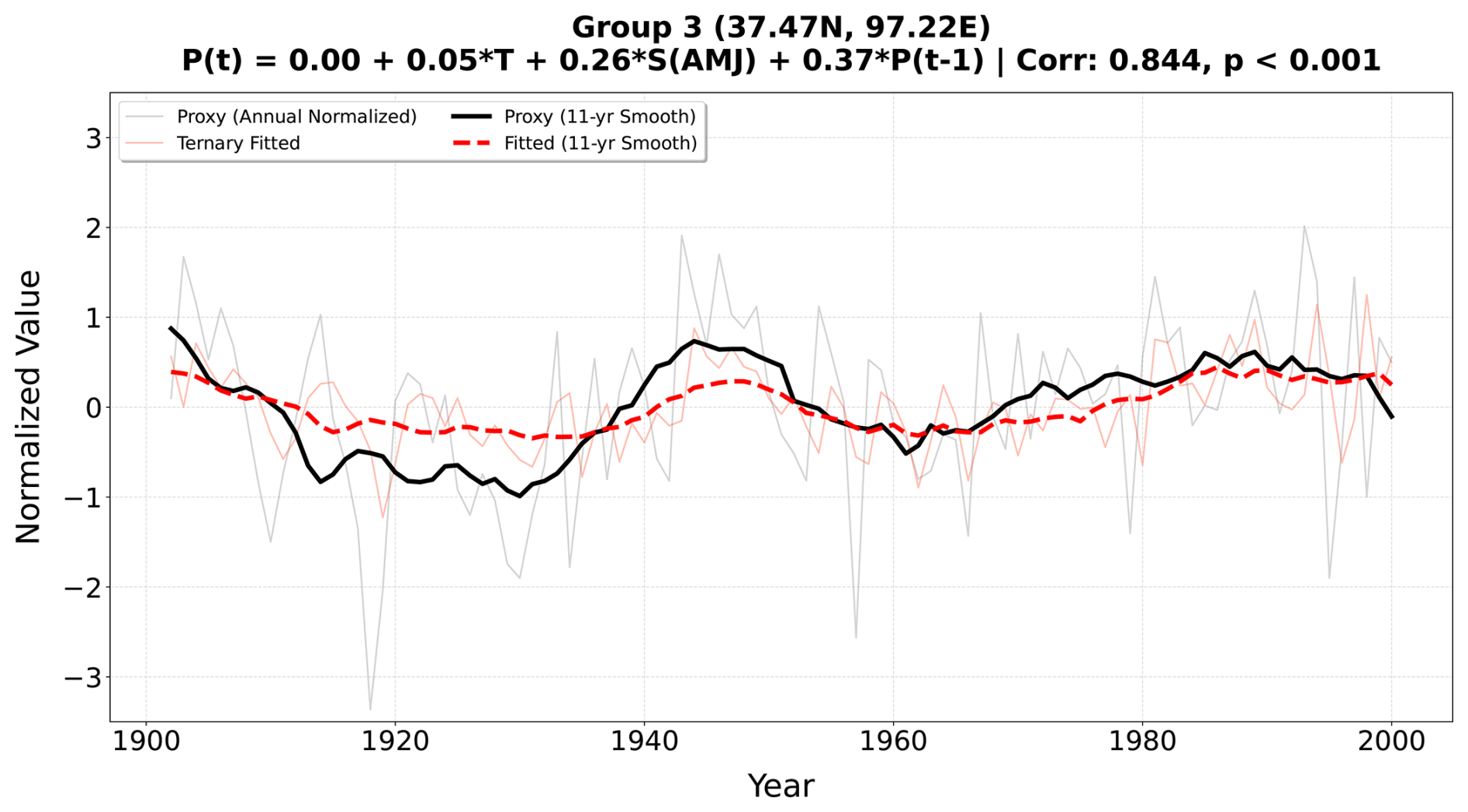
Figure 12 Temporal consistency between the actual tree-ring proxy and the TPHH-based ternary fitted series (1901–2000). The fitted series is generated via a standardized ternary regression model integrating TPHH JJA temperature (T), AMJ specific humidity (S), and lag-1 biological memory of the tree-ring proxy (P). Bold lines denote the 11-year moving average, highlighting the low-frequency correlation. See Figs. S9–S23 for all the validations across 41 proxy groups.

5 Conclusions

TPHH shows strong target-referenced reconstruction performance during 1979–2023 and close statistical agreement with available station records. Breakpoint, trend, and proxy diagnostics support regional-scale temporal plausibility, while the observationally sparse pre-1950 period and western high-elevation Plateau remain less constrained.

TPHH helps address the scarcity of high-resolution near-surface specific-humidity information over the Tibetan Plateau in the pre-satellite era. It combines the long temporal coverage of CRU_TS with the high-resolution TPMFD target fields to provide monthly $\mathrm{1}/\mathrm{30}$° × $\mathrm{1}/\mathrm{30}$° reconstructions for 1901–2023. Key validation results are summarized as follows:

1. Model performance: FourCastNet showed strong target-referenced reconstruction performance during the 1979–2023 overlap period. The nine-fold cross-validation against TPMFD yielded mean R² values of 0.989, 0.991, and 0.999 and RMSE values of 0.978 °C, 0.295 g kg⁻¹, and 1.46 hPa for temperature, specific humidity, and pressure, respectively.

2. Historical plausibility: Station-based comparisons using up to 125 pre-1979 CMA stations indicate that TPHH reproduces selected station-observed statistical characteristics. Because possible overlap with TPMFD cannot be excluded and western high-elevation stations are sparse, these comparisons do not constitute independent validation or establish uniform local accuracy.

3. Climate trends: Period-specific monthly trend maps reveal spatially heterogeneous temperature, humidity, and pressure changes across five 30-year windows. Because no full-period centennial humidity-product comparison or causal attribution was performed, the results are presented as internal TPHH trend diagnostics rather than proof of persistent wetting or monsoon intensification.

TPHH provides a candidate high-resolution historical climate dataset for studies of hydrology, glaciers, and ecosystems over the Tibetan Plateau. Users should interpret fine-scale pre-1950 variability and results over the western and central high-elevation Plateau cautiously.

6 Code and data availability

The TPHH dataset and supporting reconstruction-performance files are available at https://doi.org/10.57760/sciencedb.36169 (Chen, 2026). The release includes gridded performance-metric, DEM-sensitivity, Pettitt test, and trend data in NetCDF files. Source codes are available at https://github.com/Sawyer000/TPHH (last access: 10 September 2026) and https://doi.org/10.5281/zenodo.22690805 (Jin and Chen, 2026) with README and license files.

7 Discussion

7.1 Physical basis of TPHH's downscaling approach

The downscaling framework is data driven. FourCastNet learns nonlinear mappings between upsampled CRU_TS predictors and high-resolution TPMFD target fields, including statistical gradients associated with terrain. Its architecture and MSE loss do not explicitly impose elevation, slope, aspect, the Clausius–Clapeyron relationship, the hypsometric equation, or conservation laws. In the DEM ablation experiment, adding an explicit DEM channel changed the spatially averaged R² and IOA by less than 0.001 (Figs. S24–S29), indicating little additional predictive information under the tested configuration. Accordingly, TPHH patterns are described as terrain related and physically plausible, not physically or dynamically guaranteed.

7.2 Comparison with two other 1901–present reconstructions

Although the primary objective of TPHH is to reconstruct near-surface atmospheric humidity fields via machine-learning downscaling, this product also demonstrates advantages in air temperature reconstruction performance. Traditional reconstruction methods, such as the delta downscaling interpolation employed by Peng et al. (2019), rely heavily on the assumption of spatially continuous lapse rates. While effective in homogenous terrain, these methods treat the “terrain-climate” relationship as a static, local linear function of elevation. These frameworks are insufficient to reflect various terrain-atmosphere feedback conditions. In the complex hinterlands of the TP, where terrain governance induces various features, this method struggles to capture the high-frequency variability, leading to the “smoothing effect” observed in their results. Recent advancements by Yang et al. (2023b) introduced a deep-learning model based on generative adversarial network (GAN) to reconstruction. However, standard convolutional neural networks (CNNs) used in such studies typically operate with limited “receptive fields”. They excel at extracting local features but often fail to capture long-range dependencies, that is the critical “teleconnections” between the large-scale synoptic background and sub-regional micro-climates. As a result, while the GAN-based product improves local texture, it may lose physical consistency across the broader “total-field” when the input station data is sparse. Figure S7 shows that all three products have larger temperature RMSE in parts of complex terrain, with differing spatial patterns. TPHH has lower target-referenced RMSE than the two selected products in several high-relief regions, but this comparison against TPMFD does not establish physical consistency or identify the causal limitations of the competing methods. Due to its insufficient spatial resolution (∼10 km × 10 km), the GAN-based product even shows widespread noise in the extremely rugged southeastern TP, failing to follow the actual terrain patterns. Notably, the bias amplification of the delta-downscaling-based product in high-relief areas is entirely and substantially greater than that of TPHH. In the high-elevation central-southern TP (around 29° N, 93° E), TPHH even effectively mitigated the influence of mountainous terrain and did not display elevation-dependent bias, providing a stark contrast to the delta-downscaling-based product.

7.3 Uncertainty and prospects

Despite the advancements in downscaling reconstruction, TPHH has certain limitations. First, the reconstruction quality is inherently bounded by the temporal consistency of the predictor dataset. Although CRU_TS provides long temporal coverage, any systematic biases in the early 20th-century observational records could propagate into the TPHH product. Second, while the $\mathrm{1}/\mathrm{30}$° × $\mathrm{1}/\mathrm{30}$° resolution is a major advancement, it may still be insufficient to resolve micro-climate features in extremely narrow valleys or glaciated peaks smaller than the grid scale. Future iterations of this work will aim to incorporate multi-source predictors (e.g., paleo-climate proxies) to further constrain uncertainties in the pre-1950 observational void. The post-1979 overlap period, the 1950–1978 historical period, and the observationally sparse pre-1950 period have different levels of constraint. FourCastNet transfers statistical relationships learned from modern CRU_TS–TPMFD pairs and cannot recover mesoscale variability absent from early CRU_TS predictors. Pettitt and trend diagnostics support regional-scale temporal consistency but do not quantify pre-1950 error or provide a comprehensive uncertainty product. CMA station comparisons may overstate independence because CMA observations contributed to TPMFD, and the western and central high-elevation Plateau remain weakly constrained by direct observations. Fine-scale early-century variability in these regions should therefore be interpreted cautiously.