Normalized difference vegetation index maps of pure pixels over China for estimation of fractional vegetation cover

Fractional Vegetation Cover (FVC) is an important vegetation structure factor for applications in agriculture, forestry, ecology, etc. Due to its simplicity, the normalized difference vegetation index (NDVI)-based mixture model is widely used to estimate FVC from remotely sensed data. However, the accuracy and efficiency of FVC estimation require the precise calculation of two key parameters: the NDVI of fully covered vegetation and bare soil. Despite their importance, these two endmember NDVI values have not yet been produced as large-scale maps. Traditional statistical methods for obtaining endmember NDVI from satellite datasets highly rely on the assumption that a certain amount of pure pixels of vegetation and soil must be present, which is often invalid for many areas. This study generated 30 m resolution maps of endmember NDVI across China using the MultiVI algorithm, incorporating multi-angle remote sensing data. The quality and accuracy of the endmember NDVI maps were evaluated using various validation data, including statistically obtained pure NDVI, soil spectra from a soil library, and field-measured FVC. The NDVI values for bare soil derived from the MultiVI algorithm were consistent with those obtained from the soil spectral library. Additionally, the FVC estimated using the MultiVI-derived endmember NDVI and the VI-based mixture model exhibited reasonable accuracy compared to the field measurements. The root mean square deviation (RMSD) values for MultiVI FVC were below 0.13 in the Heihe, Hebei, and Three Gorges Reservoir regions of China. These regions include typical arid and humid zones, facilitating the evaluation of the algorithm's performance under diverse climatic conditions. Furthermore, the MultiVI FVC outperformed those calculated using the traditional statistical methods. The endmember NDVI maps provide a convenient and reliable source of key parameters for the accurate and rapid estimation of FVC at large scales. The 30 m pure NDVI maps of 2014 are publicly available at https://doi.org/10.5281/zenodo.15720622 (Zhao et al., 2024a).

1 Introduction

Fractional vegetation cover (FVC) quantitatively characterizes the horizontal density of photosynthetically active vegetation (Gutman and Ignatov, 1997). It is typically defined as the planar proportion of green vegetation to the total surface extent (Deardorff, 1978). The FVC is an essential parameter in climate and hydrologic models as it represents the spatial contribution of vegetation (Hirano et al., 2004; Gutman and Ignatov, 1998; Eriksson et al., 2006; Mölders and Olson, 2004). Accurate and high-resolution FVC products are in high demand for various studies, including climate change analysis, soil erosion assessment, land disturbance evaluation, and crop growth monitoring (Xie et al., 2011; Naqvi et al., 2013; Gan et al., 2014; Li et al., 2014; Zhang et al., 2013; Fernández-Guisuraga et al., 2021).

Remote sensing can rapidly and repeatedly observe the land surface, making estimating FVC on regional or global scales feasible. Over recent decades, tremendous efforts have been made to derive high-quality FVC from remotely sensed imagery. The published approaches for retrieving FVC can generally be summarized as follows: (i) the vegetation index (VI)-based mixture model (Gutman and Ignatov, 1998; Zeng et al., 2000; Wu et al., 2014; Mu et al., 2021; Zhao et al., 2023); (ii) spectral mixture analysis (García-Haro et al., 2005; Dimiceli et al., 2011; Guan et al., 2012); (iii) machine learning (Baret et al., 2007; Baret et al., 2013; Jia et al., 2015); and (iv) physical model (Xiao et al., 2016).

The linear mixture model is the most commonly used spectral unmixing method. It is generally utilized in surface elements evaluation such as vegetation classification, surface disturbance mapping, and evapotranspiration estimation (Li et al., 2018a; Lu et al., 2003; Cochrane and Souza, 1998). When considering only two endmembers (green vegetation and bare soil), linear mixture modelling can be employed to calculate the relative abundance of live vegetation from the mixed VI, known as the VI-based mixture model. It assumes that the VI for a particular pixel originates from a linearly weighted sum of green vegetation and bare soil, with their respective areal proportions as weighting coefficients (Gitelson et al., 2002). The mixed VI (V) of the pixel is linearly decomposed by the two endmembers, i.e., the VI of the fully vegetated (V_v) and bare soil pixel (V_s), to obtain the areal proportion of green vegetation as FVC:

$$\begin{array}{}\text{(1)}& \text{FVC}={\displaystyle \frac{V-V_{\mathrm{s}}}{V_{\mathrm{v}}-V_{\mathrm{s}}}},\end{array}$$

Table 1 Brief summary of the primary methods for determining the two pure VI values (V_v and V_s with NDVI as the default VI).

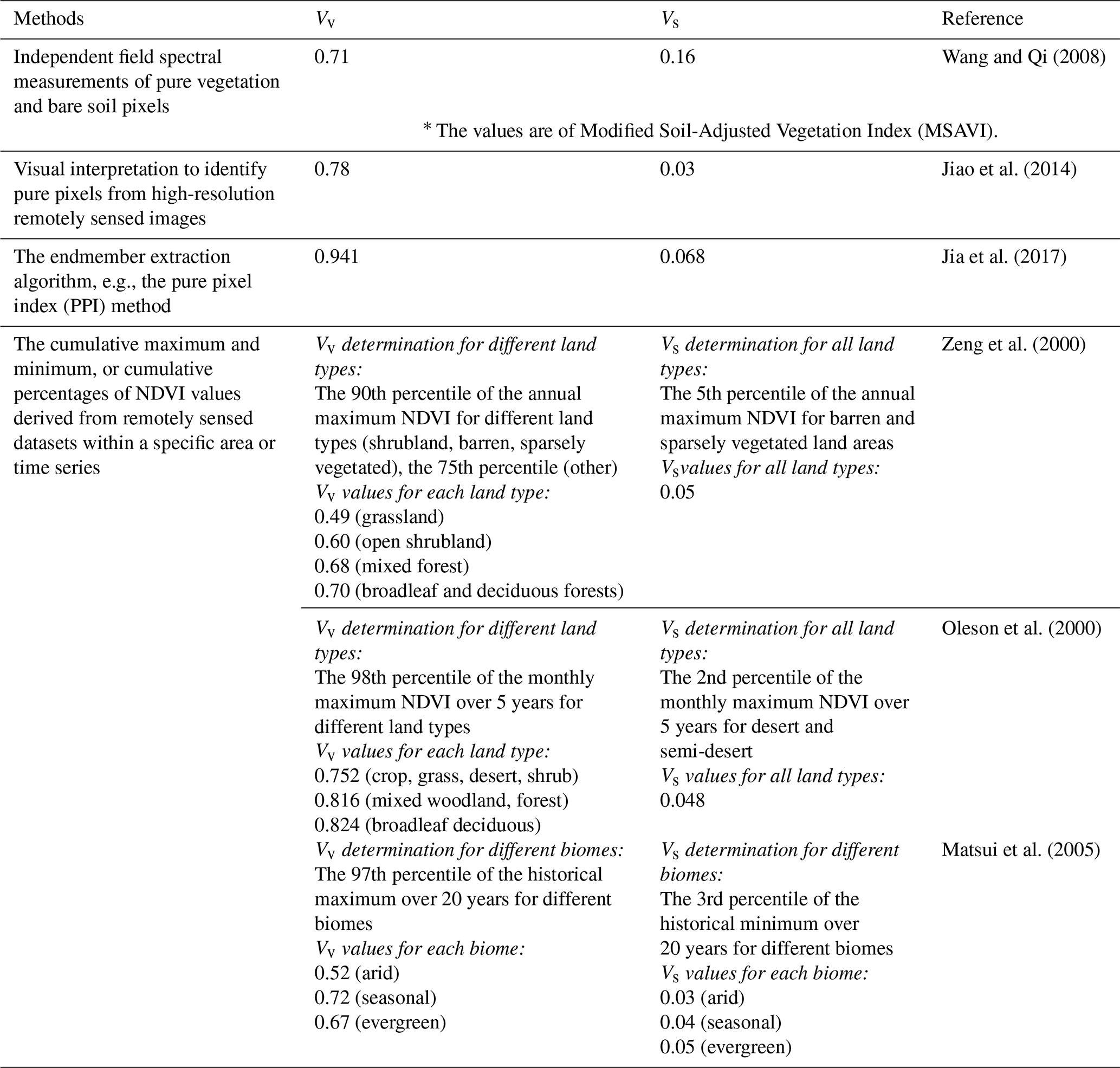
Despite being the most commonly used method for deriving FVC (Gao et al., 2020), the VI-based mixture model still requires enhancements in both accuracy and efficiency. A major limitation is the challenge of obtaining accurate values for V_v and V_s on a large scale. The “greenness” VIs that exhibit a strong linear relationship with FVC can be used in the VI-based mixture model, such as the enhanced vegetation index (EVI) and the normalized difference vegetation index (NDVI) (Song et al., 2022a). Among them, the NDVI is the primary VI used to derive FVC due to its strong correlation with vegetation structural parameters (Gutman and Ignatov, 1998). The two endmember NDVI values (hereafter referred to as pure NDVI values) are often assigned a priori, and the main methods for extracting these values, along with other pure VIs are summarized in Table 1.

Traditional methods for determining pure NDVI values have significant limitations. Collecting V_v and V_s from ground truth data or high-resolution remotely sensed imagery by extracting pure pixel values is time-consuming and often limited by data availability. These methods become ineffective when data are unavailable or there are no pure pixels in the usable dataset. The statistical method infers the two pure NDVI values from the data within a specific area or time series. It typically assumes that pixels with the lowest NDVI values represent bare soil, while those with the highest values represent pure vegetation (Gao et al., 2020). However, in arid and semiarid regions with few fully vegetated pixels, or evergreen forests with limited bare soil pixels, the statistically extracted endmember values can be significantly inaccurate (Song et al., 2017).

Additionally, statistical methods typically assign a single value of V_v or V_s for a specific region or land type. However, endmember values can vary significantly from pixel to pixel due to differences in species composition, vegetation health, moisture levels, and other factors (Jensen, 2000). In many studies, a fixed value of V_s is adopted for various soil types, as shown in Table 1, which overlooks the spatial variations in soil moisture, texture, mineralogy, organic matter, and other characteristics (Yang and Yang, 2006; Zeng et al., 2000). The NDVI values of soil samples exhibit considerable variation, ranging from 0 to 0.4, with a mean value of 0.2, which is significantly higher than the commonly used V_s value (of approximately 0.05) (Montandon and Small, 2008). Notably, the accuracy of FVC estimation is highly sensitive to variations of V_s, particularly in sparse-vegetated areas (Asrar et al., 1984; Montandon and Small, 2008). Underestimating V_s may lead to an overestimation of FVC, with errors reaching up to 20 % in grassland and shrubland regions (Montandon and Small, 2008; Ding et al., 2016). It has been demonstrated that locally derived pure NDVI values provide higher accuracy for FVC estimation, compared to using a fixed global V_s value (Donohue et al., 2014; Montandon and Small, 2008). Therefore, pixel-wise maps of endmember NDVI are essential for effectively addressing the spatial variability of plant and soil reflectance. However, such products are currently unavailable.

Recent studies have proposed an alternative method that uses multi-angle datasets from the Moderate Resolution Imaging Spectroradiometer (MODIS) to derive pixel-wise V_v and V_s (MultiVI algorithm) (Mu et al., 2018; Song et al., 2022a). The discrepancies in directional NDVI values observed from multiple viewing geometries imply vegetation structural information and soil characteristics (Chen et al., 2005; Diner et al., 1999; Deering, 1999; Verrelst et al., 2008). The MultiVI algorithm utilizes the variations from two large viewing angles to establish equations for simultaneously retrieving V_v and V_s, without assuming invariant endmember values within a scene or biome. Feasibility analysis indicated its potential to estimate high-quality, high-resolution FVC products (Song et al., 2022b). The V_v and V_s derived from the MultiVI algorithm have been used to generate 30 m/15 d FVC products, which are reported to possess satisfactory accuracy (Zhao et al., 2023). However, the accuracy of the V_v and V_s maps still requires evaluation, and strategies to optimize the MultiVI algorithm for large-scale V_v and V_s mapping are essential. Providing high-quality pure NDVI values for the VI-based mixture model will significantly improve the accuracy and efficiency of FVC estimation.

This study aims to generate and validate 30 m resolution pixel-wise V_v and V_s maps across China. These datasets can be applied to accurately calculate FVC at various resolutions on regional or national scales. The V_v and V_s maps were derived from MODIS reflectance data using the MultiVI algorithm. Subsequently, the 500 m MODIS V_v and V_s were downscaled to 30 m resolution based on land cover types (hereafter referred to as MultiVI V_v and V_s). Traditional statistical methods were employed to extract V_v and V_s from Landsat data (hereafter referred to as statistical V_v and V_s). The two sets of pure NDVI values were then compared and analysed. The generated V_s maps were validated using soil NDVI values calculated from a soil spectral library. Finally, the FVC values derived from the MultiVI algorithm and the statistical method were validated against field-measured FVC obtained from various experimental sites across China.

2 Datasets

2.1 Satellite data for V_v and V_s calculation

2.1.1 Terra/Aqua MODIS BRDF products

The MODIS Bidirectional Reflectance Distribution Function (BRDF)/Albedo Model Parameters product (MCD43A1) and its corresponding quality assessment product (MCD43A2) (https://www.earthdata.nasa.gov/data/catalog/lpcloud-mcd43a1-061, last access: 17 June 2025) are the primary datasets used to derive pure NDVI values using the MultiVI algorithm. These datasets are produced daily using atmospherically corrected, cloud-cleared input data from the Terra and Aqua satellites over 16 d at 500 m resolution. The BRDF characterizes surface anisotropic scattering as a function of illumination and viewing angles. The MCD43A1 product contains three sets of model weighting parameters, i.e., the RossThick kernel (volume-scattering kernel), LiSparseR kernel (geometric-optical kernel), and isotropic kernel parameters. These parameters can be used with the semiempirical linear kernel-driven model, known as the semiempirical RossThick-LiSparse Reciprocal (RTLSR), to calculate surface reflectance (SR) for any required viewing and illumination directions (Roujean et al., 1992; Schaaf et al., 2002). All MCD43A1 data obtained in 2014 over China were used to reconstruct the ground surface reflectance of red and near-infrared (NIR) bands at viewing zenith angles (VZAs) of 55 and 60° (see Sect. 3.1.1 for further details on the selection of angular configuration). These reflectance values were subsequently used to generate directional NDVI for the MultiVI algorithm. The quality assessment data from MCD43A2 were applied to exclude clouds, snow, water, and low-quality pixels.

2.1.2 GlobeLand30 datasets

A global land cover dataset with a 30 m resolution, known as GlobeLand30, was used to downscale the 500 m resolution pure NDVI values to 30 m. The GlobeLand30 products are available globally in three versions: 2000, 2010, and 2020, with the 2020 version being adopted for this study (https://doi.org/10.12041/geodata.140236667788805.ver1.db, National Geomatics Center of China, 2018). These products were developed and updated using cloudless or minimally cloudy multispectral images from Landsat, HJ-1, and GF-1 (Chen et al., 2014; Chen et al., 2015). Validation based on over 230 000 samples indicated a total accuracy of 85.72 % for the 2020 version of GlobeLand30, with a Kappa coefficient of 0.82. The GlobeLand30 products define bare land as having an FVC of lower than 10 %, which is stricter than the criteria used by other land cover products. This criterion helps minimize the misclassification of sparse shrubland or grassland as bare land (Liu et al., 2021). The GlobeLand30 product categorizes land cover into ten classes: six vegetation classes (i.e., cultivated land, forest, grassland, shrubland, wetland, and tundra) and four non-vegetation classes (i.e., artificial surfaces, bare land, water bodies, and perennial snow and ice) (Jun et al., 2014). The classes of wetlands, water bodies, and perennial snow and ice were grouped during the downscaling of V_v and V_s, as their pure NDVI values are generally similar (below 0).

2.2 Validation data

2.2.1 Statistical V_v and V_s

The Landsat 8 data were used to obtain V_v and V_s using statistical methods on the Google Earth Engine (GEE) platform. These statistical V_v and V_s maps were subsequently compared to the pure NDVI values derived from the MultiVI algorithm. The Landsat 8 Collection 2 SR products with a resolution of 30 m provided atmospherically corrected SR data (https://www.usgs.gov/landsat-missions/landsat-collection-2-level-2-science-products, last access: 17 June 2025). The time-series Landsat 8 SR images from 2010 to 2020 were analysed to derive statistical V_v and V_s. Pixels identified as cloud, cloud shadow, water, and snow in the Landsat 8 images were excluded using the corresponding quality assessment data.

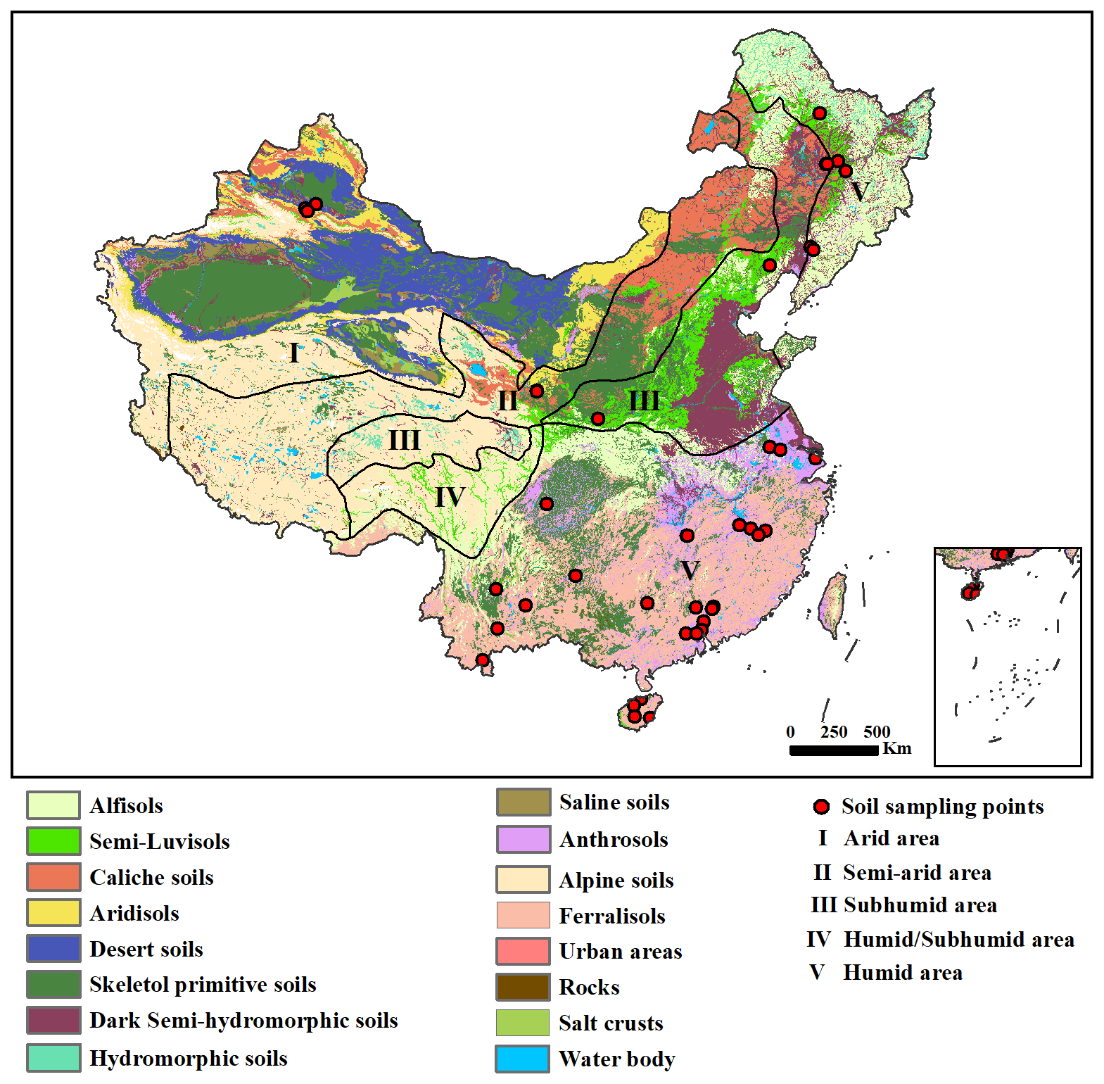
Figure 1 The spatial distribution of soil types in China. The red circle represents the locations of soil samples in the ICRAF soil spectral library. The ecological and geographical zones of China are numbered using Roman numerals.

2.2.2 Soil NDVI from the soil spectral library

The soil spectra measured at the Soil and Plant Spectral Diagnostic Laboratory of the World Agroforestry Center (ICRAF) were used to calculate soil NDVI values (https://files.isric.org/public/other/, last access: 17 June 2025), which were subsequently compared with the retrieved V_s values. The soil spectral library that includes soil samples collected from 58 countries was developed by ICRAF in collaboration with the International Soil Reference and Information Centre (ISRIC). This soil spectral library provides laboratory-measured soil spectra, along with attribute data such as geographical coordinates, horizon, and physical and chemical properties. Approximately 20 g of air-dried soil samples were passed through a 2 mm sieve, and placed into 7.4 cm diameter Duran glass Petri dishes for measurement (Garrity and Bindraban, 2006). Spectral measurements were conducted using a FieldSpec FR spectroradiometer (Analytical Spectral Devices, Boulder, CO) at wavelengths ranging from 0.35 to 2.5 µm, with 1 nm intervals (Garrity and Bindraban, 2006).

Table 2 NDVI of the soil samples collected from the soil spectral library.

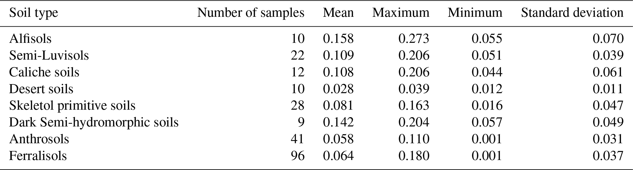
Among the soil samples in the ICRAF soil spectral library, 247 were collected in China (Fig. 1). The retrieved V_s values were constrained to be no lower than 0, consistent with the findings of most studies (Montandon and Small, 2008; Ding et al., 2016). Consequently, those samples with NDVI values below 0 were excluded, resulting in a total of 228 samples available for validation. These samples were categorized into eight soil types (Table 2) based on their collection locations and the soil type map of China (https://www.resdc.cn/data.aspx?DATAID=145, last access: 17 June 2025). Additionally, Fig. 1 illustrates the ecological and geographical zones of China, highlighting the humid and arid areas according to moisture conditions (https://www.resdc.cn/data.aspx?DATAID=125, last access: 17 June 2025).

The NDVI values of the soil samples in the ICRAF soil spectral library range from 0 to 0.273, with the majority concentrated around 0.1. The mean NDVI value for all soil samples in China is 0.077, with a standard deviation of 0.049. Desert soils exhibit the lowest NDVI values, with a maximum of 0.039. This soil type is mainly found in the arid regions of northwestern China (Fig. 1). In contrast, Alfisols have the highest NDVI values, reaching a maximum of 0.273. These soils are primarily distributed in the humid regions of northeastern and southwestern China (Fig. 1).

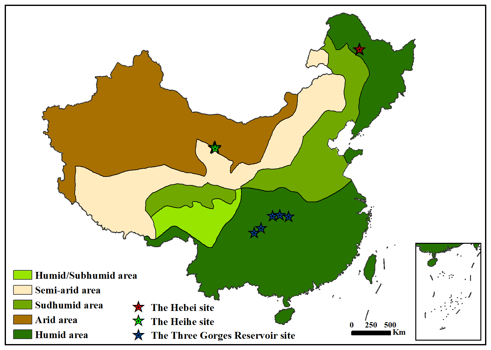
Figure 2 The ecological and geographical zones of China. The red, green, and blue pentagrams symbolize the Hebei site, the Heihe site and the Three Gorges Reservoir site, respectively.

2.2.3 Field-measured FVC

The field-measured FVC data were collected from three sites that represent typical climatic conditions in China: (i) the Hebei watershed in humid northeastern China, (ii) the Heihe River Basin in arid northwestern China, and (iii) the Three Gorges Reservoir Area in humid southwestern China. All field measurements were conducted over a complete vegetation growth cycle, with data collected approximately every 15 d. Figure 2 shows the locations of these sites.

The Hebei watershed is located in a typical black soil region of China and is mainly covered by crops. Eight sampling plots were distributed in relatively flat and uniform areas, comprising five forest plots, two grassland plots, and one cropland plot. The field measurements were conducted between 15 April and 30 October 2022. For the cropland and grassland, an unmanned aerial vehicle (UAV) was used to capture FVC images, achieving a resolution higher than 1.5 cm and covering a plot size of 100 m × 100 m. The UAV-derived FVC values were used in the subsequent validation analysis. For the forests, a digital camera was used to acquire FVC, with a plot size of 30 m. The camera was mounted on a long pole at a height of 1.5 to 2 m above the ground and took vertical photographs at regular intervals along two diagonal lines within each sampling plot (Mu et al., 2013; Li et al., 2012). Images were captured from top to bottom and bottom to top at each step to document the coverage of understory vegetation (f_up) and overstory canopy (f_down), respectively. The FVC was calculated as the weighted sum of the f_up and f_down using the following Eq. (2):

$$\begin{array}{}\text{(2)}& \text{FVC}=f_{\text{up}}+(\mathrm{1}-f_{\text{up}})\cdot f_{\text{down}},\end{array}$$

The study area in the Heihe River Basin comprises 72 % cropland, 24 % residential land, and 4 % woodland, indicating significant surface heterogeneity (Mu et al., 2015). The sampling plots, each measuring 10 m × 10 m, were exclusively located in cropland areas within the Heihe Watershed Allied Telemetry Experimental Research (HiWATER) sites, where corn was the predominant crop. The FVC measurements were conducted using a digital camera from 15 May to 14 September, 2012, encompassing the entire growing season.

The Three Gorges Reservoir Area is situated in the mid-upper reaches of the Yangtze River. Five representative small river basins were selected for vegetation monitoring within this region. Seasonal trajectories of vegetation cover were recorded using UAVs every 2 weeks from 15 August 2021 to 1 August 2022. Each small river basin contained a sampling plot of approximately 100 m × 100 m, distributed in a relatively flat and homogeneous area. The primary vegetation types included orchards, forests, and shrubland. The UAV images had a resolution of higher than 1.5 cm.

A Half-Gaussian Fitting algorithm (HAGFVC) was used to calculate FVC from UAV-acquired images, resulting in a minimal mean bias error (MBE) and root mean square error (RMSE) of less than 0.04 (Li et al., 2018b). The digital images captured by hand-held cameras were processed using a shadow-resistant algorithm (SHAR-LABFVC) to extract FVC, achieving an RMSE of approximately 0.025 (Song et al., 2015).

3 Methods

3.1 MultiVI algorithm for retrieving the pure NDVI maps

3.1.1 Theory

The MultiVI algorithm uses multi-angle remotely sensed observations to retrieve V_v and V_s. It defines the directional vegetation cover, F(θ), which represents the FVC at the VZA θ. A nonlinear coefficient, k, is introduced in the VI-based mixture model. This coefficient accommodates the potential nonlinear relationship between FVC and NDVI, as shown in Eq. (3) (Xiao and Moody, 2005; Jiapaer et al., 2011; Choudhury et al., 1994; Mu et al., 2024):

$$\begin{array}{}\text{(3)}& F\left(\mathit{\theta }\right)={\left({\displaystyle \frac{V\left(\mathit{\theta }\right)-V_{\mathrm{s}}}{V_{\mathrm{v}}-V_{\mathrm{s}}}}\right)}^k,\end{array}$$

where V(θ) is the NDVI observed at VZA θ. The directional gap fraction model can be expressed as Eq. (4) (Nilson, 1971):

$$\begin{array}{}\text{(4)}& P\left(\mathit{\theta }\right)=e^{-G\left(\mathit{\theta }\right)\cdot \mathrm{\Omega }\left(\mathit{\theta }\right)\cdot \text{LAI}/\cos \mathit{\theta }},\end{array}$$

Here, P(θ) denotes the directional gap fraction, G(θ) is the mean projection of unit foliage area (Goel and Strebel, 1984), Ω(θ) is the clumping index, and LAI represents the leaf area index. The directional FVC and gap fraction exhibit a complementary relationship, such that the sum of F(θ) and P(θ) equals 1. Therefore, Eqs. (3) and (4) can be combined as follows:

$$\begin{array}{}\text{(5)}& \mathrm{1}-{\left({\displaystyle \frac{V\left(\mathit{\theta }\right)-V_{\mathrm{s}}}{V_{\mathrm{v}}-V_{\mathrm{s}}}}\right)}^k=e^{-G\left(\mathit{\theta }\right)\cdot \mathrm{\Omega }\left(\mathit{\theta }\right)\cdot \text{LAI}/\cos \mathit{\theta }},\end{array}$$

The G(θ) in Eq. (5) is often assumed to be constant at large VZAs around 57.5°, despite variations in leaf angle distributions (Leblanc et al., 1999; He et al., 2012; Song et al., 2017; Mu et al., 2018; Weiss et al., 2004; Roujean et al., 1992). Furthermore, the variation of G(θ)⋅Ω(θ) is significantly smaller than the angular variation of cosθ at large VZAs (Mu et al., 2018). Since the LAI is also independent of VZA, $G\left(\mathit{\theta }\right)\cdot \mathrm{\Omega }\left(\mathit{\theta }\right)\cdot \text{LAI}$ can be assumed to be invariant at large VZAs around 57.5°. The angular effects of V_v and V_s are negligible (Escadafal and Huete, 1991; Mu et al., 2018). By using pairs of observations at large VZAs around 57.5° and eliminating angle-invariant parameters, Eq. (5) can be reorganized as:

$$\begin{array}{}\text{(6)}& {\left(\mathrm{1}-{\left({\displaystyle \frac{V\left({\mathit{\theta }}_i\right)-V_{\mathrm{s}}}{V_{\mathrm{v}}-V_{\mathrm{s}}}}\right)}^k\right)}^{\cos {\mathit{\theta }}_i}={\left(\mathrm{1}-{\left({\displaystyle \frac{V\left({\mathit{\theta }}_j\right)-V_{\mathrm{s}}}{V_{\mathrm{v}}-V_{\mathrm{s}}}}\right)}^k\right)}^{\cos {\mathit{\theta }}_j},\end{array}$$

where the subscripts “i” and “j” represent pairs of large VZAs around 57.5°. The combination of 55 and 60° in the forward viewing directions was identified as the optimal angular configuration. This selection is attributed to its minimal influence on G(θ) and the high quality of angular remote sensing observations (Mu et al., 2018). These angles were used to formulate equations for estimating V_v and V_s:

$$\begin{array}{}\text{(7)}& {\left(\mathrm{1}-{\left({\displaystyle \frac{V\left(\mathrm{55}\mathit{°}\right)-V_{\mathrm{s}}}{V_{\mathrm{v}}-V_{\mathrm{s}}}}\right)}^k\right)}^{\cos \mathrm{55}\mathit{°}}={\left(\mathrm{1}-{\left({\displaystyle \frac{V\left(\mathrm{60}\mathit{°}\right)-V_{\mathrm{s}}}{V_{\mathrm{v}}-V_{\mathrm{s}}}}\right)}^k\right)}^{\cos \mathrm{60}\mathit{°}},\end{array}$$

The unknown parameters V_v, V_s, and k for a given pixel can be derived using at least three pairs of angular observations at VZAs of 55 and 60° to solve Eq. (7).

3.1.2 Implementation

The observed NDVI used to solve Eq. (7) should exhibit distinct variations to ensure stable results (Mu et al., 2018). This study used observations from different periods to construct appropriate equations for each pixel. The V_v and V_s were independently retrieved to enhance accuracy by applying high and low NDVI values, respectively. The minimum and maximum NDVI values for each pixel in 2014 were used as statistical boundaries. This approach ensured that the derived V_s values remained below the annual minimum, while the derived V_v values exceeded the annual maximum. Furthermore, empirical boundaries for V_s ([0.01, 0.3]) and V_v ([0.6, 1.0]) were applied to constrain the retrieval, preventing the upper limit of V_s from exceeding 0.3 and the lower limit of V_v from falling below 0.6 (Montandon and Small, 2008). This flexible approach integrates statistical boundaries for V_v and V_s, while allowing for reasonable intra-variability within each land cover type.

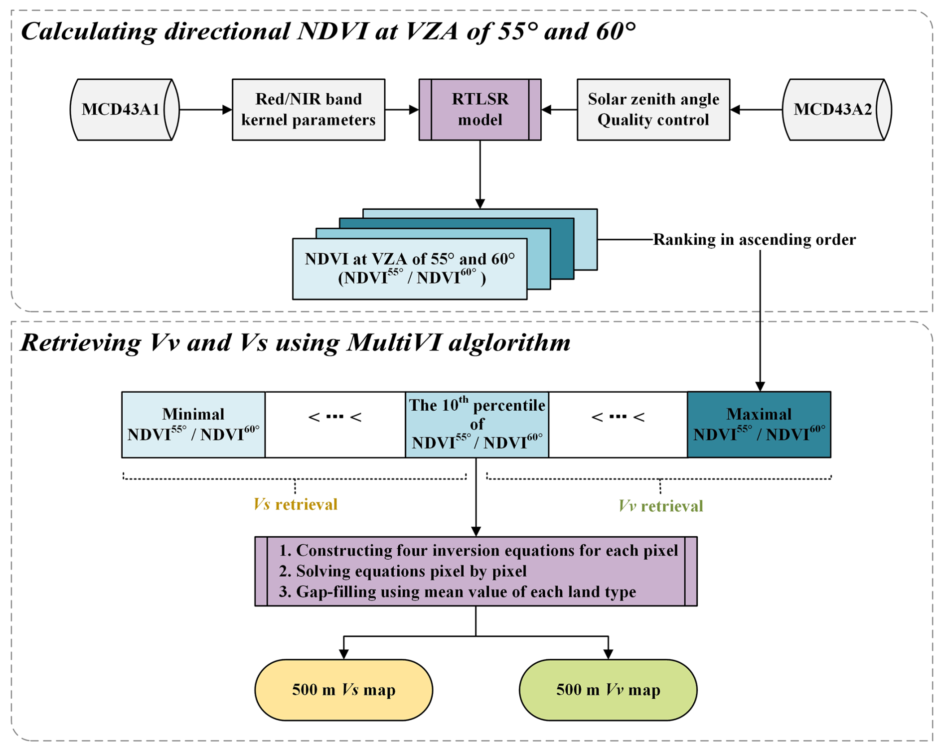
Figure 3 The scheme of the MultiVI algorithm to derive 500 m pure NDVI values from MODIS BRDF products.

Figure 3 illustrates the steps for using the MultiVI algorithm to derive 500 m pure NDVI values from the MODIS BRDF products:

1. Daily directional NDVI values at VZA of 55 and 60° were calculated for each pixel throughout the year using the semi-empirical RTLSR model;

2. NDVI pairs at VZA of 55 and 60° were ranked in ascending order based on the values at 55° VZA for the entire year;

3. The annual NDVI value sequence was divided into two groups based on the 10th percentile. The NDVI values below the 10th percentile were used to retrieve V_s using Eq. (7), while the remaining 90 % were used to retrieve V_v;

4. The 25th, 50th, 75th, and 100th percentiles of the NDVI pairs in each group were selected to construct inversion equations (Eq. 7) for each pixel. The unknown parameters V_v, V_s, and k were numerically solved using the least squares method;

5. For a small number of invalid pixels due to limited observations, gap filling was performed based on the MODIS land cover data (MCD12Q1). The mean values of V_v and V_s corresponding to the same land cover type were used to fill these gaps.

3.2 NDVI unmixing for downscaling the 500 m V_v and V_s

The 500 m V_v and V_s were downscaled to a 30 m resolution using NDVI unmixing to facilitate fine-scale FVC estimation. It was assumed that the same land cover type within each MODIS pixel was assigned the same V_v and V_s values. The 500 m V_v and V_s were considered as linear combinations of the 30 m V_v and V_s values within that MODIS pixel, with weights determined by the areal proportions of land cover types.

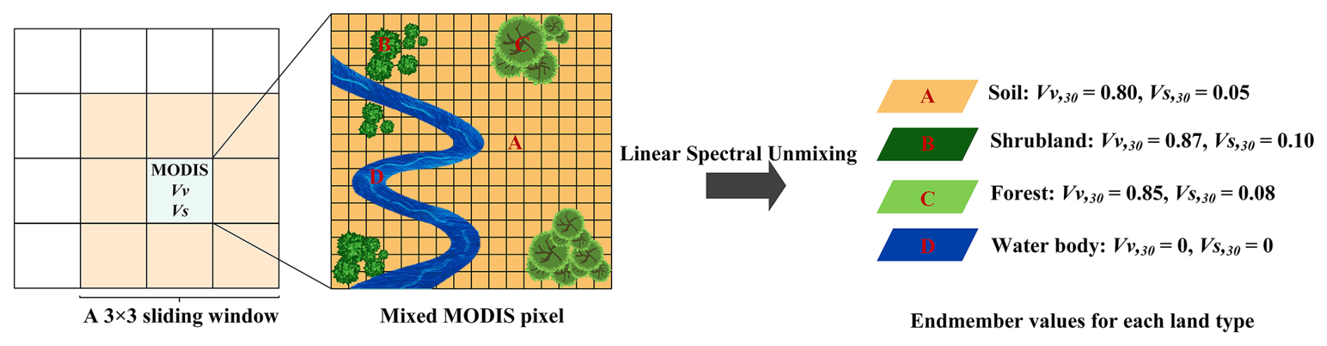
Figure 4 The schematic diagram for downscaling the 500 m MultiVI V_v and V_s to 30 m resolution based on the GlobeLand30 product.

The downscaling process utilized seven land cover types from the GlobeLand30 product, specifically four vegetation classes (cultivated land, forest, grassland, shrubland, and tundra), a grouped water surface category (wetland, water body, and permanent snow and ice), bare land, and artificial surfaces. A 3 × 3 sliding window with a step size of one MODIS pixel was employed to construct an overdetermined system of unmixing equations for the MODIS pixel at (x,y), as shown in Eq. (8) for downscaling V_v:

$$\begin{array}{}\text{(8)}& \left\{\begin{array}{l}{V}_{\mathrm{v},\text{modis},x-\mathrm{1},y-\mathrm{1}}={\sum }_{i=\mathrm{1}}^n{P}_{i,x-\mathrm{1},y-\mathrm{1}}{V}_{\mathrm{v},i,x,y}\\ V_{\mathrm{v},\text{modis},x-\mathrm{1},y}={\sum }_{i=\mathrm{1}}^n{P}_{i,x-\mathrm{1},y}{V}_{\mathrm{v},i,x,y}\\ V_{\mathrm{v},\text{modis},x-\mathrm{1},y+\mathrm{1}}={\sum }_{i=\mathrm{1}}^m{P}_{i,x-\mathrm{1},y+\mathrm{1}}{V}_{\mathrm{v},i,x,y}\\ V_{\mathrm{v},\text{modis},x,y-\mathrm{1}}={\sum }_{i=\mathrm{1}}^n{P}_{i,x,y-\mathrm{1}}{V}_{\mathrm{v},i,x,y}\\ V_{\mathrm{v},\text{modis},x,y}={\sum }_{i=\mathrm{1}}^n{P}_{i,x,y}{V}_{\mathrm{v},i,x,y}\\ V_{\mathrm{v},\text{modis},x,y+\mathrm{1}}={\sum }_{i=\mathrm{1}}^n{P}_{i,x,y+\mathrm{1}}{V}_{\mathrm{v},i,x,y}\\ V_{\mathrm{v},\text{modis},x+\mathrm{1},y-\mathrm{1}}={\sum }_{i=\mathrm{1}}^n{P}_{i,x+\mathrm{1},y-\mathrm{1}}{V}_{\mathrm{v},i,x,y}\\ V_{\mathrm{v},\text{modis},x+\mathrm{1},y}={\sum }_{i=\mathrm{1}}^n{P}_{i,x+\mathrm{1},y}{V}_{\mathrm{v},i,x,y}\\ V_{\mathrm{v},\text{modis},x+\mathrm{1},y+\mathrm{1}}={\sum }_{i=\mathrm{1}}^n{P}_{i,x+\mathrm{1},y+\mathrm{1}}{V}_{\mathrm{v},i,x,y}\end{array}\right.\end{array}$$

where $V_{\mathrm{v},\text{modis},x,y}$ represents the V_v of a target MODIS pixel, i.e., the central MODIS pixel of the sliding window. Each equation corresponds to a neighbouring MODIS pixel in the 3 × 3 window. $P_{i,x,y}$ signifies the areal proportion of the ith land cover type within this MODIS pixel, indicating its area-weighted contribution. $V_{\mathrm{v},i,x,y}$ denotes the V_v for the ith land cover type, which is assumed to be constant across the sliding window for each land cover type i, and is an unknown to be estimated.

By solving these equations, the V_v value was inferred for each land cover type. The derived values of $V_{\mathrm{v},i,x,y}$ were then assigned as the V_v for all the 30 m pixels of land cover type i within the MODIS pixel at (x,y). The same procedure was applied to obtain $V_{\mathrm{s},i,x,y}$. Figure 4 illustrates the method for downscaling 500 m pure NDVI values to 30 m resolution.

3.3 Assessment and validation

3.3.1 Comparison with statistical methods

Statistical methods were used to generate 30 m statistical V_v and V_s in 2014 across China using Landsat 8 data, which were then compared with the MultiVI V_v and V_s. The statistical method utilized Landsat 8 data from 2010 to 2020, processed on the Google Earth Engine (GEE) platform. The pixel-wise maximum and minimum NDVI values from 2010 to 2020 were set as the V_v and V_s, respectively. The statistical V_v and V_s were compared with the MultiVI V_v and V_s to assess their differences in spatial patterns and magnitudes.

3.3.2 Comparison with soil NDVI from the soil spectral library

The soil spectra obtained from the soil spectral library were convolved to the red and NIR bands using the spectral response functions of MODIS. The convolved soil spectra were then used to calculate the soil NDVI for comparison with the retrieved V_s. The MultiVI V_s and statistical V_s were averaged for each soil type to facilitate comparison with the soil NDVI. Additionally, the uncertainties in the estimated FVC caused by intra-class variability in V_s were assessed for each soil type.

3.3.3 Assessment with field-measured FVC

The field-measured FVC at the Hebei, Heihe, and Three Gorges Reservoir sites were used to assess the estimated FVC derived from the MultiVI V_v/V_s and that from the statistical V_v/V_s. The Landsat 8 NDVI time series were smoothed using a harmonic model (Zhao et al., 2023). The NDVI was generated at half-monthly intervals to coincide with the observation times of the field measurements. Subsequently, the NDVI was converted to FVC using the VI-based mixture model and the retrieved V_v and V_s.

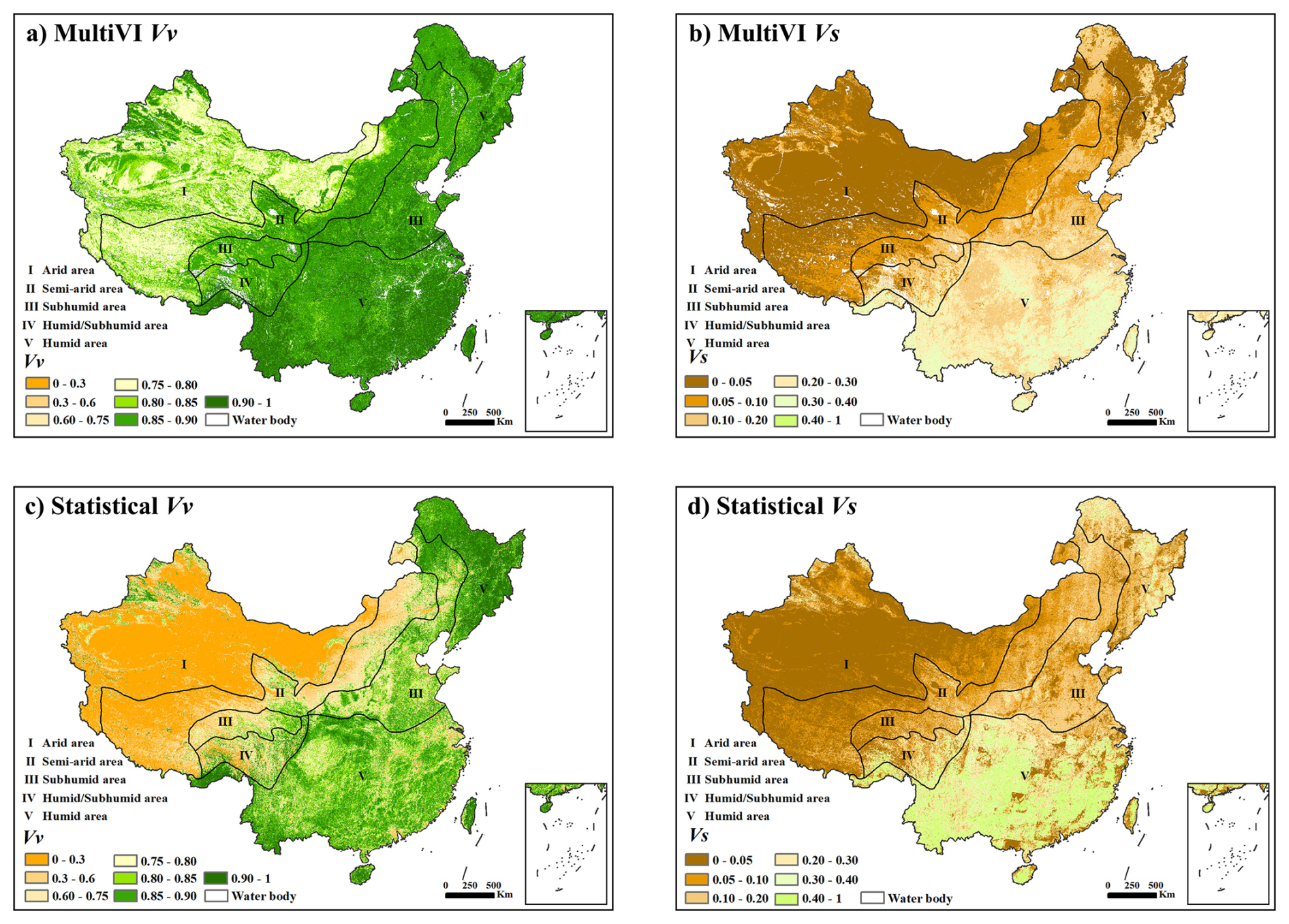
Figure 5 The spatial distributions of V_v and V_s generated using the MultiVI algorithm and the statistical method, respectively.

The plot sizes for ground measurements ranged from 10 to 100 m, and various spatial matching strategies were implemented to enhance the consistency between ground observations and satellite-derived FVC. For the cropland and grassland plots at the Heihe site, as well as all plots at the Three Gorges Reservoir site, UAV measurements with a plot size of 100 m × 100 m were utilized. To minimize potential edge effects and ensure spatial correspondence, UAV-derived FVC was processed to orthophotos, calculated over the central 90 m × 90 m area and compared with the average FVC from the co-located 3 × 3 block of 30 m satellite pixels. For forest plots measuring 30 m × 30 m at the Heihe site, satellite FVC was averaged over a surrounding 3 × 3 window to account for potential geolocation uncertainty and scale mismatch, following the methodology of Weiss et al. (Weiss et al., 2007). Given the high spatial homogeneity of the Heihe site, direct pixel-to-plot comparisons were also performed by matching the ground-measured FVC from the 10 m × 10 m plots with the corresponding 30 m satellite pixels. The correlation coefficient (R²) and the root mean square deviation (RMSD) were used to assess the relationship and differences between the field-measured FVC and the estimated FVC, respectively.

4 Results

4.1 Maps of the MultiVI V_v and V_s

Figure 5 shows the V_v and V_s maps generated using the MultiVI algorithm (Fig. 5a and b) and the statistical method (Fig. 5c and d). The MultiVI V_v and V_s maps demonstrate smooth distributions, whereas the statistical V_v and V_s maps exhibit noticeable stripes along the borders of the Landsat 8 imagery tiles. The spatial patterns of pure NDVI values derived from the MultiVI algorithm and the statistical method show similar trends, predominantly influenced by moisture conditions. Specifically, the humid and sub-humid areas of southeastern China are characterized by elevated pure NDVI values, while the arid and semi-arid regions of northwestern China are dominated by lower values.

The statistical V_v are generally lower than the MultiVI V_v in most areas, particularly in semi-arid and arid regions. In northwestern China, which is primarily covered by grasslands, bare lands, and deserts, the statistical method yields NDVI values of less than 0.3 for pure vegetation pixels (Fig. 3b). These values are significantly lower than the V_v values reported in most studies (Table 1).

Table 3 MultiVI V_v and V_s for different land types.

Table 3 presents the MultiVI V_v and V_s values across various land types. The mean V_v values range from 0.817 to 0.909, while the mean V_s values range from 0.074 to 0.287. Both MultiVI V_v and V_s exhibit consistent patterns across different land types, indicating that vegetation with higher V_v values tends to also exhibit higher V_s values. The shrublands show the lowest values, whereas evergreen needleleaf forests exhibit the highest values. The forests generally have higher values than other land types, with evergreen forests surpassing broadleaf forests. In contrast, grasslands and shrublands have lower values compared to other land types. The standard deviation values for V_s are greater than those for V_v.

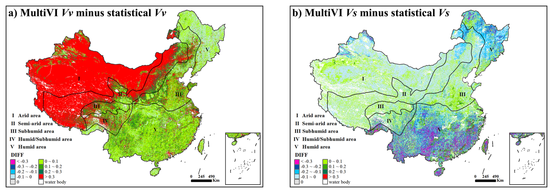
Figure 6 The difference maps between the MultiVI NDVI and statistical NDVI for pure vegetation and bare soil.

The spatial patterns of the MultiVI V_s exhibit distinct variations across different soil types and demonstrate a closer alignment with the actual soil distribution in China (Fig. 1) when compared to the statistical V_s. The MultiVI V_s are generally lower than the statistical V_s, especially in the densely vegetated areas of southeastern China. In these humid regions, the statistical V_s values exceed 0.4, where evergreen vegetation predominates and shows few bare lands (Fig. 3d). These values, which exceed 0.4, are notably higher than the generally accepted soil NDVI values (Table 1).

Figure 6 shows the differences between the MultiVI V_v/V_s and the statistical V_v/V_s. The largest discrepancies are observed in regions lacking pure pixels, i.e., the arid areas where pure vegetation pixels are absent for V_v estimation, and the humid areas where bare soil pixels are lacking for V_s estimation.

In the sparse grasslands of northwestern China, the MultiVI V_v are significantly higher than the statistical V_v, with a bias exceeding 0.3 (Fig. 6a). In most humid or subhumid areas of southeastern China, the difference between the two sets of V_v values is generally within ± 0.1. For relatively sparse vegetation, such as grasslands and croplands, the MultiVI V_v are slightly higher than the statistical V_v. However, in forested areas, the MultiVI V_v are slightly lower than the statistical V_v.

In the densely vegetated forests of southeastern China, the MultiVI V_s are markedly lower than the statistical V_s, with a bias of less than −0.3 (Fig. 6b). In arid regions, the MultiVI V_s values are slightly lower than the statistical V_s values in sparse grasslands and bare lands, but higher in oases, with biases of approximately −0.1 and +0.1, respectively.

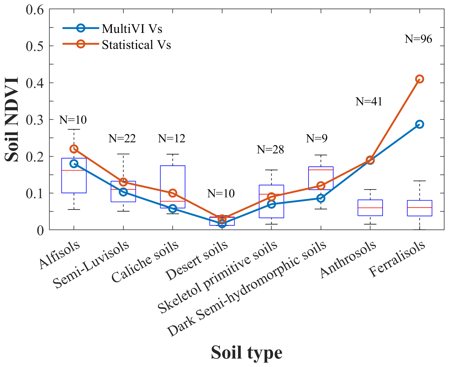
Figure 7 The boxplot of the soil NDVI from the ICRAF soil library for each soil type. Each boxplot features a central red line representing the median. The N above the box indicates the number of sampling plots for each soil type. The lower and upper edges of the box denote the 25th and 75th percentiles, respectively. The whiskers are extended to the most extreme data points, excluding outliers. The blue and red lines denote the median values of the MultiVI V_s and statistical Vs, respectively.

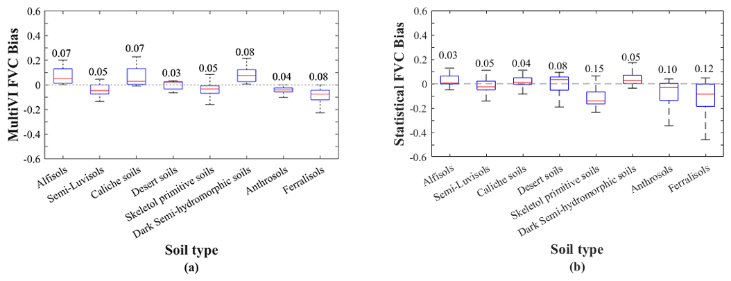
Figure 8 The bias in FVC estimation across different soil types using different V_s values. The FVC bias represents the difference between the estimated FVC using (a) MultiVI V_s or (b) statistical V_s and the reference FVC derived from soil NDVI in the ICRAF soil library. The number above each box indicates the mean absolute bias of FVC for each soil type. The lower and upper edges of the box denote the 25th and 75th percentiles, respectively. The whiskers are extended to the most extreme data points, excluding outliers.

4.2 Evaluation with soil NDVI from the soil spectral library

Figure 7 shows the MultiVI V_s and statistical V_s in comparison to the soil NDVI derived from the ICRAF soil library. For Alfisols and Semi-Luvisols, the median of the MultiVI V_s closely aligns with the median NDVI of the corresponding soil samples. In contrast, the median statistical V_s tend to slightly overestimate the soil NDVI. For Desert soils and Skeletol primitive soils, the median of the statistical V_s is closer to the soil NDVI, while the MultiVI V_s exhibit a slight underestimation. Both the median values of the MultiVI and the statistical V_s are lower than the median NDVI for Dark Semi-hydromorphic soils, with a bias of approximately 0.1. Soil samples of Anthrosols and Ferralisols are primarily distributed in the humid, densely vegetated regions of southeastern China, which results in relatively high NDVI values. For these soil types, the MultiVI V_s show an overestimation when compared to the median NDVI values, with biases of approximately 0.15 for Anthrosols and 0.2 for Ferralisols. For Ferralisols, this overestimation is more pronounced in the statistically derived V_s, with biases exceeding 0.3.

Figure 8 illustrates the bias between the MultiVI FVC and the statistical FVC compared to the reference FVC estimated using soil NDVI from the ICRAF soil library. The FVC bias represents the difference between the MultiVI FVC (Fig. 8a) or statistical FVC (Fig. 8b) and the reference FVC. The reference FVC was estimated using the ICRAF soil NDVI in combination with either MultiVI V_v (Fig. 8a) or statistical V_v (Fig. 8b).

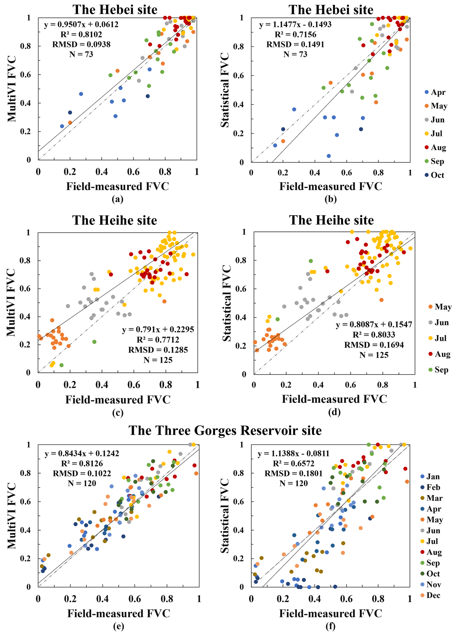
Figure 9 Scatterplots of the MultiVI FVC and the statistical FVC versus the field-measured FVC. N is the number of samples.

For the MultiVI FVC, the median bias is within ± 0.05, and the mean absolute values consistently remain below 0.1 across all soil types. The overestimation of the MultiVI V_s yields a slight underestimation of FVC for Anthrosols and Ferralisols. The overestimations of 0.15 and 0.2 in MultiVI V_s leads to underestimations of approximately 0.04 and 0.08 in FVC for Anthrosols and Ferralisols, respectively, both of which are located in densely vegetated areas. Conversely, the slight underestimation of MultiVI V_s relative to soil NDVI results in overestimations of 0.07 and 0.08 in FVC for Caliche soils and Dark Semi-hydromorphic soils, respectively. The statistical method performs better than the MultiVI algorithm for the Alfisols, Caliche soils, and Dark Semi-hydromorphic soils. The underestimation of statistical FVC exceeds −0.1 for Skeletol primitive soils, Anthrosols, and Ferralisols.

4.3 Accuracy of FVC estimation

Figure 9 depicts scatterplots that compare field-measured FVC with FVC derived from the MultiVI V_v/V_s and the statistical V_v/V_s across three sites: the Hebei site (Fig. 9a and b), the Heihe site (Fig. 9c and d), and the Three Gorges Reservoir site (Fig. 9e and f).

The MultiVI FVC demonstrates superior accuracy relative to the statistical FVC at the Hebei site, exhibiting a lower RMSD of 0.0938 for the MultiVI FVC, in contrast to 0.1491 for the statistical FVC. Additionally, the MultiVI FVC has a higher R² of 0.8121, compared to 0.7156 for the statistical FVC. Both the MultiVI FVC and the statistical FVC show saturation effects for high FVC values at the Hebei site during the summer season (Fig. 9a and b). However, the MultiVI FVC aligns more closely with the 1:1 line, particularly during the non-growing seasons, specifically in April, September, and October.

The MultiVI FVC exhibits a slightly lower RMSD of 0.1285 compared to 0.1694 for the statistical FVC at the Heihe site. However, it has a lower R² of 0.7712 versus 0.8033 for the statistical FVC. The majority of the data points depicted in Fig. 9c and d are situated above the 1:1 line, indicating an overestimation in both the MultiVI FVC and the statistical FVC.

At the Three Gorges Reservoir site, the MultiVI FVC also demonstrates superior accuracy, as indicated by an RMSD of 0.1022, in contrast to 0.1801 for the statistical FVC. Additionally, the correlation between the MultiVI FVC and field-measured FVC is significantly higher (R² = 0.8162) than that of the statistical FVC (R² = 0.6572). As illustrated in Fig. 9f, a part of the statistical FVC data points are saturated at high values and drop to zero at low values, indicating that the statistical method suffers from an underestimation of V_v and an overestimation of V_s in humid areas.

Figure 9 also reveals seasonal patterns in the errors of FVC derived from the VI-based mixture model. At the Hebei site, larger deviations from the 1:1 line are observed in April and October, indicating greater uncertainty during the early growth and senescence stages. At the Heihe site, the FVC shows the largest error in June, particularly when 0.2 < FVC < 0.5. In the Three Gorges Reservoir area, the most significant FVC errors occur during winter months (January to February) and summer months (July to September). The seasonal patterns in the errors of the statistical FVC are generally more pronounced than those of the MultiVI FVC.

5 Discussion

The VI-based mixture model is widely used to estimate FVC due to its ease of implementation. The model's simplicity is primarily attributed to the preselection of two critical parameters: the NDVI of bare soil (V_s) and that of pure vegetation (V_v). These parameters are essential for the model's performance and have a significant impact on its accuracy. The traditional statistical method for obtaining V_v and V_s assumes the existence of pure pixels, either spatially or temporally. This method employed extreme values from regional or temporal datasets to represent V_v and V_s. However, this approach has two significant limitations: (1) pure pixels may be absent in certain ecosystems, such as evergreen forests, where bare soil pixels are lacking, or in bare lands, where pure vegetation pixels are absent; (2) the V_v and V_s can vary from pixel to pixel, yet the traditional statistical method often assigns a single value for an entire region or land type.

The global soil spectral library was used to calibrate V_s and to account for its spatial variability (Montandon and Small, 2008). Although this method improves the accuracy of FVC estimation compared to using a single V_s value across large regions, it is limited in that it only considers soil variability within the spectral library and fails to address the spectral differences among individual pixels. An alternative approach is to use each pixel's historical lowest NDVI values as V_s to ensure pixel-wise variability. In practice, V_s is influenced not only by mineral soil properties but also by non-photosynthetic vegetation (NPV), biological residues, and surface litter. A previous study reported that the NDVI of NPV endmembers is generally higher than that of bare soil, with differences reaching up to 0.4 in some cases (Tian et al., 2021). This suggests that V_s may vary even within the same soil type. Land cover classification can partially account for such heterogeneity, and land cover data were utilized as a practical proxy to disaggregate 500 m V_s to a 30 m resolution in this study.

Figure 7 further illustrates that the retrieved V_s values deviate from the soil NDVI in humid regions. The most significant discrepancy is observed in the soil types of Anthrosols and Ferralisols, which are prevalent in the humid areas of southern China. This discrepancy is likely attributed to their relatively high NDVI values, and the presence of surface litter and biological residues. However, the overestimation of MultiVI V_s in these areas has a limited impact on the FVC estimation (Fig. 8a), with the resulting FVC bias generally less than 0.1. Previous studies have also indicated that the influence of V_s on FVC estimation is more pronounced in areas with low NDVI values, such as grasslands and croplands/natural vegetation areas, compared to regions with high NDVI values (Ding et al., 2016).

In this study, statistical maps of V_v and V_s were generated using a common statistical criterion (Sect. 3.3.1). Empirical NDVI for fully vegetated pixels is typically reported to exceed 0.5 in most studies (Gao et al., 2020; Zeng et al., 2000; Montandon and Small, 2008), whereas the statistical V_v are observed to be below 0.3 in arid regions of China (Fig. 5a). Except for these extreme areas, the statistical method demonstrates comparable accuracy to the MultiVI algorithm (Figs. 7, 8, and 9c, d). The simple statistical methods face challenges in identifying appropriate NDVI values when pure pixels are lacking. In contrast, several studies have adopted more sophisticated statistical approaches to produce accurate FVC estimates across various ecosystems (Donohue and Renzullo, 2025; Donohue et al., 2018). These enhanced statistical methods take into account the inherent characteristics of vegetation in different ecosystems, employing separate thresholds to determine endmembers in arid and vegetated areas, respectively. The use of spatially adaptive thresholding facilitates the acquisition of reasonable endmembers and achieves high FVC accuracy, with a RMSE of approximately 0.1 (Donohue and Renzullo, 2025).

The errors in the FVC estimated from the VI-based mixture model vary across seasons and are more pronounced during periods of low vegetation cover. Figure 9 shows that FVC errors are generally larger in early spring and winter, particularly for low FVC values. This seasonal pattern can be explained by the sensitivity of FVC estimation to NDVI values in the 0.2–0.4 range (Montandon and Small, 2008). Within this interval, small errors in V_s can lead to systematic overestimations of FVC, especially over grasslands and shrublands. During peak growing seasons, when NDVI values exceed 0.7, the model estimates become more stable and less sensitive to endmember NDVI values. Furthermore, the saturation of FVC estimates, resulting from an underestimation of V_v and an overestimation of V_s, typically influences winter and summer periods (Fig. 9f).

The MultiVI algorithm, which uses multi-angle data to retrieve V_v and V_s, has demonstrated effectiveness in estimating FVC and has been applied to generate FVC time series on a national scale (Song et al., 2022a; Zhao et al., 2023). This algorithm retrieves angle-invariant NDVI values for endmembers using observations from two large VZAs. In this study, the retrieval strategy of the MultiVI algorithm was optimized through the construction of well-posed equations based on NDVI time series. Additionally, the statistical values of V_v and V_s were incorporated as boundary constraints during the equation-solving process. The downscaling procedure integrates a 30 m land cover product, which introduces finer spatial detail to describe the sub-pixel heterogeneity within MODIS pixels. Our downscaling approach applies the assumption that the 30 m pixels of the same land cover type share constant V_v and V_s values within a localized 3 × 3 window of 500 m MODIS pixels. This assumption may introduce uncertainty when significant soil type variation exists within the 3 × 3 MODIS window (1.5 km × 1.5 km). Despite the simplifications involved, the comparison with the 500 m results shows that the downscaled 30 m V_s values achieve comparable accuracy (Song et al., 2022b). The downscaling process introduces minimal changes to the endmember values (Song et al., 2022b). Considering the increasing demand for high spatial and temporal resolution applications, providing 30 m endmember products is of practical significance.

As a critical vegetation parameter, FVC is frequently demanded in various studies, serving as an input for models or as fundamental data for ecological analyses. The VI-based mixture is one of the simplest methods for converting remotely sensed images into FVC products, provided that the pure NDVI values are obtained beforehand. However, the two essential parameters in the VI-based model, V_v and V_s, currently lack standardized and reliable data sources. The newly generated 30 m V_v and V_s maps address this gap. Users can calculate accurate FVC values flexibly using the MultiVI V_v and V_s with their NDVI to meet specific requirements.

6 Data availability

The 30 m MultiVI V_v and V_s maps for 2014 are available at https://doi.org/10.5281/zenodo.15720622 (Zhao et al., 2024a). The Supplement produced the 30 m MultiVI V_v and V_s for 2018 and 2022 (available at https://doi.org/10.5281/zenodo.17463344, Zhao et al., 2024b) and evaluates their interannual stability. All V_v and V_s data are stored in GeoTIFF files using the WGS-84 (World Geodetic System 1984) coordinate system with UTM (Universal Transverse Mercator) projection. The data are categorized into tiles based on a latitude size of 5° and a longitude size of 6°. The file names consist of 18 characters following these rules: North-South latitude abbreviation (1 digit) + 6° zone number (2 digits) + “_” + starting latitude (2 digits) + “_” + product time (4 digits) + “_” + resolution (3 digits) + “_” + data attribute (2 digits). Additionally, each image contains a pure NDVI value band ranging from 0 to 100, with invalid values or water surfaces labelled as NaN. The 500 m MultiVI V_v and V_s maps are also publicly available at https://doi.org/10.5281/zenodo.15597968 (Zhao et al., 2024c).

7 Conclusion

This study demonstrates the feasibility of generating pixel-wise NDVI for fully vegetated area (V_v) and bare soil (V_s) for the VI-based mixture model. In this study, 30 m resolution maps of pure NDVI values for the year 2014 were produced for China using multi-angle remotely sensed data from MODIS and land cover datasets from Globeland30. The assessment and validation of the V_v and V_s maps were conducted from three aspects: (1) comparing the MultiVI V_v and V_s maps with those generated using the statistical method; (2) comparing the derived V_s with reference soil NDVI from the ICRAF soil spectral library; and (3) validating the accuracy of FVC calculated from the pure NDVI values against field-measured FVC. Our findings reveal the urgent need for reliable V_v and V_s per pixel for large-area FVC production. Traditional statistical methods are impractical to achieve this goal due to their reliance on pure pixels. The MultiVI algorithm has proven to be a viable solution, yielding V_v and V_s with a more reliable spatial pattern and magnitude than statistical methods. The MultiVI V_s is closely aligned with soil NDVI across various soil types in China. Furthermore, the FVC estimated using the MultiVI V_v and V_s demonstrated improved accuracy in comparison to those derived from the statistical V_v and V_s, with RMSD values around 0.1 and R² values near 0.8 for all validation sites. Moreover, the products generated in this study show broad applicability across a variety of climate zones and soil types.

The MultiVI V_v and V_s maps provide essential parameters for FVC estimation using the widely adopted VI-based mixture model, which is known for its ease of use and reasonable accuracy. Hence, these derived V_v and V_s maps are anticipated to facilitate the estimation of fine-resolution, high-frequency FVC with reliable quality at large scales.