Radiative sensitivity quantified by a new set of radiation flux kernels based on the ECMWF Reanalysis v5 (ERA5)

Radiative sensitivity, i.e., the response of the radiative flux to climate perturbations, is essential to understanding climate change and variability. The sensitivity kernels computed by radiative transfer models have been broadly used for assessing the climate forcing and feedbacks for global warming. As these assessments are largely focused on the top of atmosphere (TOA) radiation budget, less attention has been paid to the surface radiation budget or the associated surface radiative sensitivity kernels. Based on the fifth generation European Center for Medium-Range Weather Forecasts atmospheric reanalysis (ERA5), we produce a new set of radiative kernels for both the TOA and surface radiative fluxes, which is made available at https://doi.org/10.17632/vmg3s67568 (Huang and Huang, 2023). By comparing these with other published radiative kernels, we find that the TOA kernels are generally in agreement in terms of global mean radiative sensitivity and analyzed overall feedback strength. The unexplained residual in the radiation closure tests is found to be generally within 10 % of the total feedback, no matter which kernel dataset is used. The uncertainty in the TOA feedbacks caused by inter-kernel differences, as measured by the standard deviation of the global mean feedback parameter value, is much smaller than the inter-climate model spread of the feedback values. However, we find relatively larger discrepancies in the surface kernels. The newly generated ERA5 kernel outperforms many other datasets in closing the surface energy budget, achieving a radiation closure comparable to the TOA feedback decomposition, which confirms the validity of the kernel method for the surface radiation budget analysis. In addition, by investigating the ERA5 kernel values computed from the atmospheric states of different years, we notice some apparent interannual differences, which demonstrates the dependence of radiative sensitivities on the mean climate state and partly explains the inter-dataset kernel value differences. In this paper, we provide a detailed description of how ERA5 kernels are generated and considerations to ensure proper use of them in feedback quantifications.

1 Introduction

Radiative kernels measure the sensitivity of radiative fluxes to the perturbation of feedback variables, such as temperature, water vapor, albedo and cloud (e.g., Soden and Held, 2006; Huang et al., 2007; Shell et al., 2008; Previdi, 2010; Zelinka et al., 2012; Block and Mauritsen, 2013; Yue et al., 2016; Huang et al., 2017; Pendergrass et al., 2018; Thorsen et al., 2018; Kramer et al., 2019b; Smith et al., 2020). Compared to the partial radiative perturbation method (e.g., Wetherald and Manabe, 1988), which is precise but computationally expensive, the kernel method deploys a set of precalculated radiative kernels with simple arithmetic multiplications in feedback quantification and thus is computationally highly efficient, which has greatly facilitated the analysis of radiative feedbacks in global climate models (GCMs) (e.g., Soden and Held, 2006; Soden et al., 2008; Jonko et al., 2012; Vial et al., 2013; Zhang and Huang, 2014; Dong et al., 2020; Zelinka et al., 2020; Chao and Dessler, 2021) as well as in observations (e.g., Dessler, 2010; Kolly and Huang, 2018; Zhang et al., 2019; H. Huang et al., 2021). These analyses have helped dissect and understand the climate sensitivity differences among the GCMs, such as those in Coupled Model Intercomparison Projects CMIP5 (Taylor et al., 2012) and CMIP6 (Eyring et al., 2016). For example, Zelinka et al. (2020) attributed the higher climate sensitivity in the CMIP6 models to their more positive extratropical cloud feedback. The kernel-enabled feedback analyses have also provided insights into the energetics of the climate variations such as the El Niño and Southern Oscillation (ENSO, e.g., Dessler et al., 2010; Kolly and Huang, 2018; H. Huang et al., 2021), the Madden–Julian Oscillation (MJO, e.g., Zhang et al., 2019), and the Arctic sea ice interannual variability (e.g., Huang et al., 2019), despite the approximate nature of the kernel method and the known limits of its accuracy (e.g., Colman and Mcavaney, 1997; Huang and Huang, 2021).

Multiple sets of radiative kernels have been developed to date, using different radiation codes and based on different atmospheric state datasets ranging from GCMs to global reanalysis and satellite datasets, for both non-cloud variables (e.g., Soden and Held, 2006; Shell et al., 2008; Huang et al., 2017; Thorsen et al., 2018; Bright and O'Halloran, 2019; Donohoe et al., 2020) and cloud properties (e.g., Zelinka et al., 2012; Zhou et al., 2013; Yue et al., 2016; Zhang et al., 2021; Zhou et al., 2022). As the conventional feedback analyses are mostly concerned with the radiation energy budget change at the top of the atmosphere (TOA), most existing kernels have been developed and tested to address that need, i.e., to measure the feedback contributions to the TOA radiation changes. Although the radiative sensitivity depends on the atmospheric states as well as the radiative transfer codes used to compute the kernel values (e.g., Collins et al., 2006; Huang and Wang, 2019; Pincus et al., 2020), it has been noted that the global mean TOA feedback quantification is insensitive to which kernel dataset is used, as the diagnosed feedback values are close to each other when measured by different kernel datasets (e.g., Soden et al., 2008; Jonko et al., 2012; Vial et al., 2013; Zelinka et al., 2020). However, as there is increasing interest in regional climate change and associated feedback (e.g., Kolly and Huang, 2018; Huang et al., 2019; Zhang et al., 2019), it becomes important to know how the kernels (dis)agree at regional scales. The generation of the global radiative kernels usually requires radiative transfer computation based on a large number of instantaneous atmospheric profiles. Due to this computational cost, many kernel datasets are generated based on the atmospheric data from an arbitrary calendar year. Given the known interannual climate differences, e.g., between El Niño to La Niña years, this warrants investigations to ascertain whether the kernels may differ in important ways for regional feedback assessments.

On the other hand, fewer feedback studies have addressed the surface radiation budget, although its importance has been recognized for such problems as the precipitation change (Previdi, 2010; Pendergrass and Hartmann, 2014; Myhre et al., 2018) and oceanic energy transport (e.g., Zhang and Huang, 2014; Huang et al., 2017). The surface budget analysis requires the use of surface kernels, which are not always available from the published kernel datasets. Few of them have been subject to intercomparisons or rigorous validation. As explained below in this paper, the computation and use of them require different care to the TOA kernels. Possibly due to the lack of such recognition, there exist considerable discrepancies between the existing surface kernels, and some surface-budget-centered analyses reported alarmingly large non-closure in their radiation budget analyses (e.g., Vargas Zeppetello et al., 2019), calling into question the validity of the kernel method for surface radiation budget analysis. Hence, we are motivated to examine the radiative sensitivity quantified by different kernels, especially for the surface budget.

In this work, we produce a new set of radiative kernels for both the TOA and surface radiation fluxes based on the fifth generation European Center for Medium-Range Weather Forecasts atmospheric reanalysis (ERA5, Hersbach et al., 2020), which demonstrates superior accuracy in the quantification of various atmospheric states (e.g., Graham et al., 2019; Wright et al., 2020), and document the key considerations in the kernel computation procedure. We intercompare the kernels computed from ERA5 to the other previously generated ones and investigate the interannual variation in the kernel values due to their atmospheric state dependency. In addition, applying a selected set of kernels to analyzing the feedback in the CMIP6 models, we intercompare the discrepancies in quantified feedbacks across the GCMs and across different kernels.

2 Construction of ERA5 radiative kernels

2.1 Radiative transfer model and atmospheric dataset

We use the GCM version of the rapid radiative transfer model (RRTMG) (Mlawer et al., 1997) to calculate the radiative kernels. RRTMG conducts radiative transfer calculations in 16 longwave (LW) spectral bands and 14 shortwave (SW) bands. The accuracy of this model has been extensively validated against the line-by-line calculations (e.g., Collins et al., 2006).

Input data required by RRTMG, including surface pressure, skin temperature, air temperature, water vapor, albedo, ozone concentration, cloud fraction, cloud liquid water content and cloud ice content, are taken from the instantaneous (as opposed to monthly mean) data of ERA5, with a horizontal resolution of 2.5^∘ by 2.5^∘ and 37 vertical pressure levels between 1 and 1000 hPa. To ensure the accuracy of radiative kernels in the upper atmosphere (Smith et al., 2020), we patch five layers of the US standard profile above 1 hPa in the LW calculations. Other required input variables, such as the effective radii of cloud liquid droplets and ice crystals are taken from the 3-hourly synoptic TOA and surface fluxes and the cloud product of the Clouds and Earth's Radiant Energy System (CERES) (Doelling et al., 2013) with a horizontal resolution of 1^∘ and then interpolated to the same resolution as the ERA5 data (2.5^∘). A random cloud overlapping scheme is used in our all-sky calculation. Sensitivity tests have been conducted to determine the necessary temporal sampling for a proper representation of the diurnal cycle, and 6-hourly and 3-hourly instantaneous profiles are adopted for LW and SW radiative transfer calculations, respectively, to limit the root-mean-squared error in the computed diurnal mean flux biases to less than 1 %.

2.2 Radiative kernel computation

Radiative kernels in essence measure the change in radiative flux to unit perturbation of atmospheric variables, i.e., $\frac{\partial R}{\partial X}$, where R is either the upwelling irradiance flux at the TOA or upwelling and downwelling irradiance flux at the surface, X represents the aforementioned feedback variables, K_X is the radiative kernel of variable X. Note that for each radiative flux, K_X varies with the time and geographic and vertical locations of the perturbed variable and is in general a four-dimensional (4D) data array. Note also that all radiative fluxes and kernel values are defined as downward positive.

Following previous studies, we compute non-cloud radiative kernels including the LW kernels of surface temperature (T_s), air temperature (T_a) and water vapor (WV LW), and the SW kernels of surface albedo (ALB) and water vapor (WV SW). To calculate the kernels, we use the partial radiative perturbation experiments, conducting two radiative transfer computations, one without perturbation (control run) and the other with a perturbation of one atmospheric variable; the difference between these two computations is used to calculate the radiative kernel value. In both experiments, the upward, downward and net radiative fluxes at TOA and the surface are saved at each time instance and location. Then ΔR₀ can be obtained by differencing the saved radiative fluxes between the perturbed and unperturbed experiments. Dividing ΔR₀ with the perturbation of variable X (ΔX₀), the instantaneous radiative kernel K_X is calculated as

$$\begin{array}{}\text{(1)}& K_X={\displaystyle \frac{\mathrm{\Delta }{R}_{\mathrm{0}}}{\mathrm{\Delta }{X}_{\mathrm{0}}}}.\end{array}$$

Applying such perturbation computations to all the relevant variables (see the Appendix for a detailed discussion of the procedure), we obtain instantaneous radiative kernels of these dimensionalities: the surface temperature and albedo kernels are 3D arrays (time; latitude: 73; longitude: 144), and the air temperature and water vapor kernels are 4D arrays (time; level: 37; latitude: 73; longitude: 144).

To account for possible interannual variability in the radiative kernel values, we compute the kernels using atmospheric data of 5 calendar years: from the year 2011 to the year 2015. Among these years, 2011 is a strong La Niña year, and 2015 is a strong El Niño year. Monthly or annual mean kernels are then averaged from the instantaneous computations. For example, the LW annual mean kernel of 2011 is obtained as $K=\frac{\mathrm{1}}{\mathrm{365}\cdot \mathrm{4}}\sum _{i=\mathrm{1}}^{\mathrm{365}\cdot \mathrm{4}}{K}_i$ (365 is the number of days of a year and 4 is because 6-hourly data are used for LW calculations) and the SW kernels, $K=\frac{\mathrm{1}}{\mathrm{365}\cdot \mathrm{8}}\sum _{i=\mathrm{1}}^{\mathrm{365}\cdot \mathrm{8}}{K}_i$ (8 is because 3-hourly data are used for SW calculations), where the index i represents the time slices included in the averaging. A similar averaging procedure is applied to monthly mean kernels. The analyses in this work are based on multi-year averaged monthly mean kernels if not otherwise stated.

3 Characterization of ERA5 kernels

In this section, we first present the all-sky TOA and surface radiative sensitivity kernels quantified from the ERA5 in Figs. 1 to 4 (see the clear-sky kernels in Figs. S1 and S2 in the Supplement). The atmospheric radiation flux kernels, i.e., the change in radiation flux convergence in the atmosphere due to the perturbation of feedback variables and measured by differencing TOA and surface kernels, are shown in Figs. S3 and S4 for interested readers. Then, we compare ERA5 kernels with the other kernel datasets, and we examine the interannual variability in the ERA5 kernel values, due to the dependency of radiative sensitivity on the background atmospheric state.

3.1 Distribution of radiative sensitivity

Figure 1 summarizes the spatial distribution of all-sky ERA5 kernels for TOA and the surface, and Fig. 2 illustrates the vertical cross-sections of zonal mean air temperature, water vapor LW and water vapor SW kernels in all sky (see Figs. S1 and S2 for results in clear sky). For the surface temperature kernels, an increase in surface temperature leads to more upwelling longwave radiation (i.e., OLR) both at the surface and TOA; therefore the kernel is negative. The TOA flux sensitivity in clear sky (Fig. S1a) is stronger than that in all sky (Fig. 1a) due to the absence of cloud, and the value increases with latitude, due to the decreasing concentration of water vapor from the tropics to the poles. The all-sky TOA sensitivity is strongly influenced by clouds, showing, for example, the fingerprint of the Intertropical Convergence Zone (ITCZ) in the tropical oceans (Fig. 1a). The locations with less atmospheric absorption due to less water vapor or cloud, e.g., the Tibetan Plateau and Sahara regions, show relatively stronger sensitivity (Fig. 1a). For the surface flux kernels, the increase in surface temperature enhances the upward emission according to the Planck function, and thus the distribution follows that of surface temperature for both clear sky and all sky (Fig. 1b).

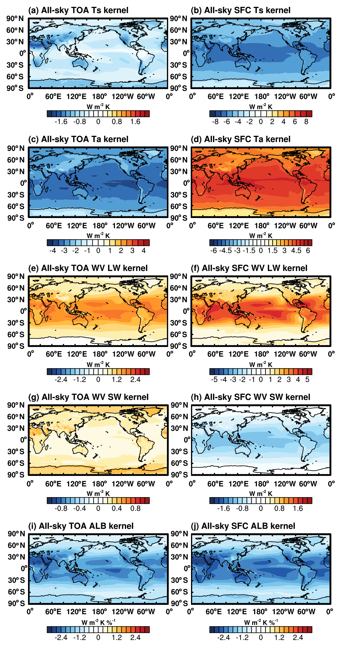
Figure 1 All-sky (left) TOA and (right) surface ERA5 kernels of (a, b) surface temperature (T_s), (c, d) air temperature (T_a), (e, f) water vapor longwave (WV LW), (g, h) water vapor shortwave (WV SW) and (i, j) surface albedo (ALB). Note that for T_a, WV LW and WV SW kernels, vertically integrated values are shown, which represents the sensitivity of radiative flux to a whole-column atmospheric perturbation. Note that the color bar ranges differ among panels.

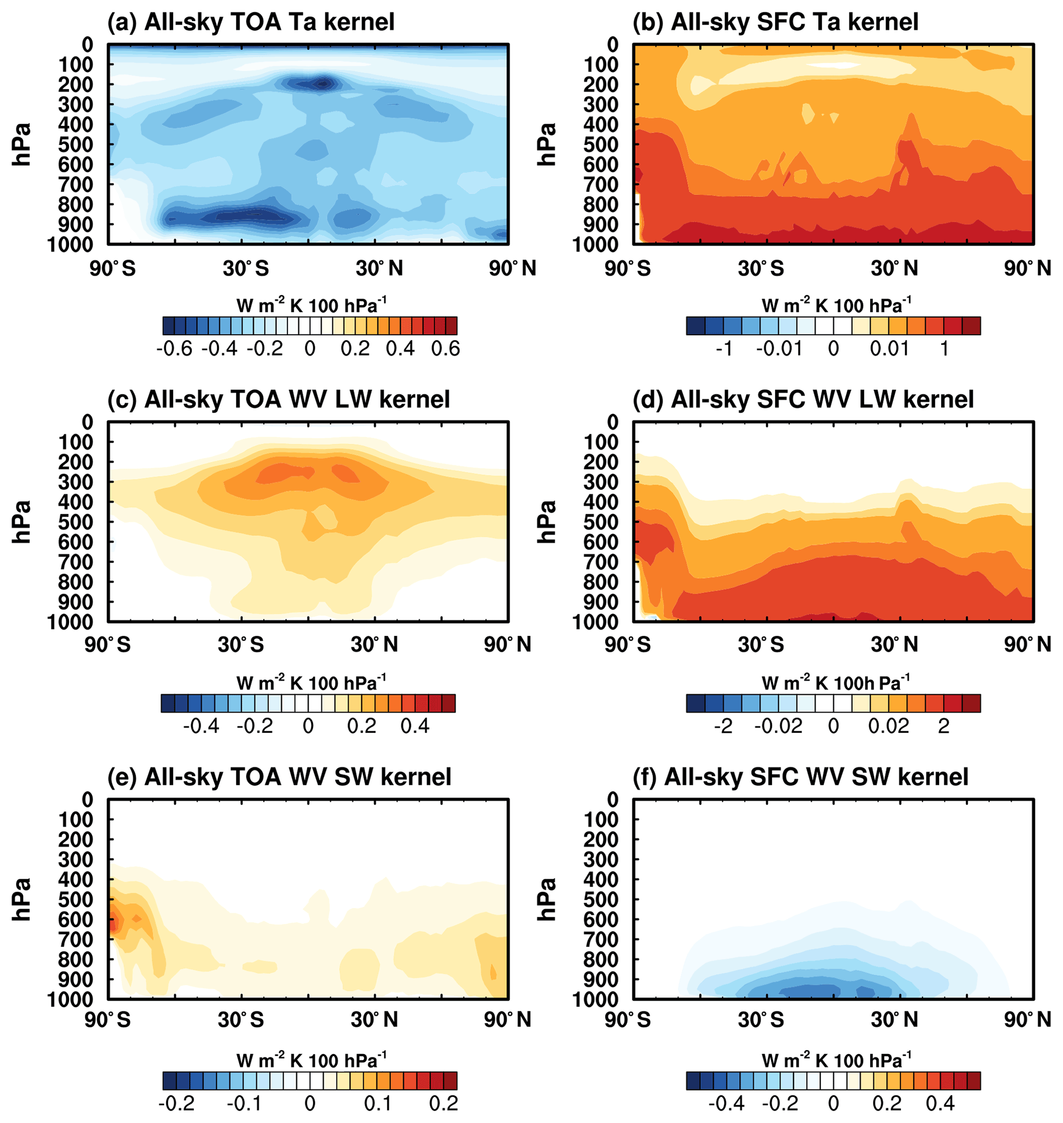
Figure 2 All-sky (left) TOA and (right) surface ERA5 vertically resolved and zonally averaged kernels of (a, b) air temperature (T_a), (c, d) water vapor longwave (WV LW) and (e, f) water vapor shortwave (WV SW); units: W m⁻² K⁻¹ 100 hPa⁻¹. Note that nonlinear color bars are used for surface air temperature and water vapor LW kernels and that the color bar ranges differ among panels.

For air temperature kernels, the increase in air temperature increases the OLR at TOA and also the downwelling flux at the surface, so the TOA and surface kernels take negative and positive signs, respectively. The TOA kernel has maximum values in the tropics, due to the higher air temperature (Planck function) and more abundant cloud and water vapor (higher emissivity) there, and generally decreases in magnitude with latitude (Fig. 1c). Unlike the TOA flux kernel, which shows comparable sensitivity to air temperature at nearly all vertical levels, the surface flux is mainly sensitive to the bottom layers (Fig. 2b).

For water vapor LW kernels, an increase in water vapor reduces OLR at TOA and increases downwelling radiation at the surface, so that the TOA and surface kernels are both positive in sign. The vertically integrated kernel values (Fig. 1e and f) generally follow the temperature distribution, for example, decreasing in magnitude with latitude. In both cases, the kernel magnitude is dampened by clouds in all sky. The vertically resolved kernels show a maximum sensitivity of TOA flux to the upper troposphere (Fig. 2c) and maximum sensitivity of surface flux to the bottom layers (Fig. 2d). In terms of the atmospheric radiation (the convergence of the TOA and surface radiation fluxes in the atmosphere), the increase in water vapor concentration absorbs more LW in the upper troposphere than what it emits, but the opposite is true in the lower troposphere (Fig. S4c). Such features were discussed in previous works (e.g., Huang et al., 2007).

For water vapor SW kernels, an increase in water vapor absorbs solar radiation and thus reduces both the upwelling (reflected) SW flux at TOA and the downwelling SW flux at the surface. As a result, the two kernels take positive and negative signs, respectively. Note that the magnitude of the SW kernels is much weaker than that of the LW kernels because water vapor absorbs the LW flux more significantly than the SW flux. One noticeable feature of the TOA kernel in clear sky (Fig. S1g) is that the magnitude over the land is stronger than that over the ocean because the relatively higher albedo over the land reflects more SW radiation and thus enhances the absorption by the water vapor in the atmosphere. For this reason, over reflective surfaces such as the Sahara and the Tibetan Plateau as well as the poles, the sensitivity is maximized. Unlike the TOA kernel, the distribution of surface kernel follows the distribution of background water vapor concentration, with noticeable dampening by clouds (Figs. 1h and 2f).

For surface albedo kernels, an increase in surface albedo leads to more upwelling (reflected) SW flux both at the surface and TOA; therefore, the kernel is of negative sign. In clear sky, the sensitivity strength follows the pattern of solar insolation, with some local maxima, e.g., in the Sahara and the Tibetan Plateau (Fig. S1i and j) due to the relatively lower water vapor concentration. In all sky, the distribution is again influenced by cloud patterns; for example, in the ITCZ region, the strength is much reduced as clouds reduce the solar radiation reaching the surface and thus the sensitivity to surface albedo change (Fig. 1i and j).

3.2 Comparison of ERA5 kernels with other datasets

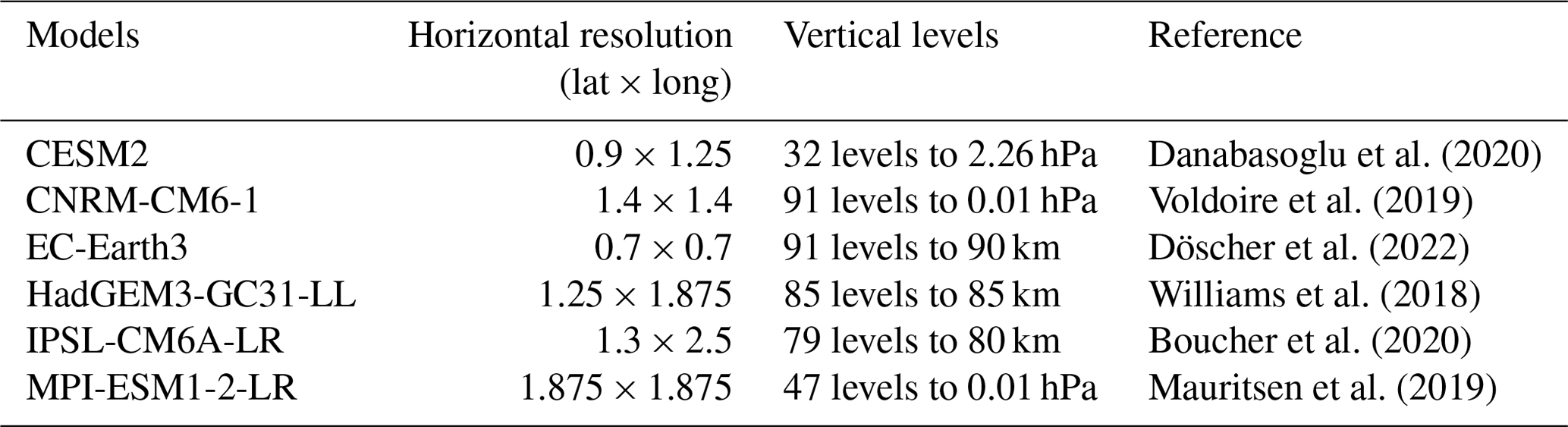
To examine the discrepancies between different kernel datasets, we select six previously published ones for comparison. Table 1 summarizes their resolutions and the datasets based on which they are computed, including the GCMs (GFDL kernel, Soden et al., 2008; CAM3 kernel, Shell et al., 2008; CAM5 kernel, Pendergrass et al., 2018; HadGEM3 kernel, Smith et al., 2020), a global reanalysis (ERAi kernel, Huang et al., 2017) and satellite observations of cloud fields from CloudSat/CALIPSO combined with thermodynamic fields from reanalyses (Kramer et al., 2019b). This list is meant to be representative instead of exhaustive.

Table 1 Summary of radiative kernels compared in this work. Datasets with ^* only have TOA kernels.

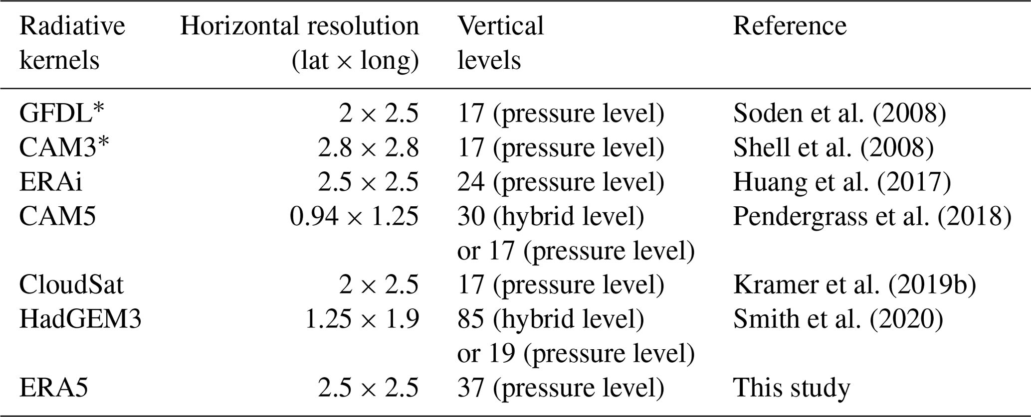
To facilitate an intercomparison, these kernel datasets are interpolated to the same horizontal and vertical resolutions as those of the ERA5 kernel when illustrated in Figs. 3 and 4 (see Figs. S5 and S6 for clear sky) and are uploaded to the same data repository of ERA5 kernels. Note that the CAM5 and HadGEM3 kernels have two versions, with one defined at the raw hybrid levels and the other interpolated to pressure levels. To retain the accuracy of them as much as possible, the hybrid level version is used for the interpolation and comparison in Figs. 3 and 4, while in Sect. 4, the pressure level version is used for quantifying the feedbacks of CMIP6 models. The GFDL and CAM3 kernels are only available for TOA fluxes and are excluded for surface kernel comparisons.

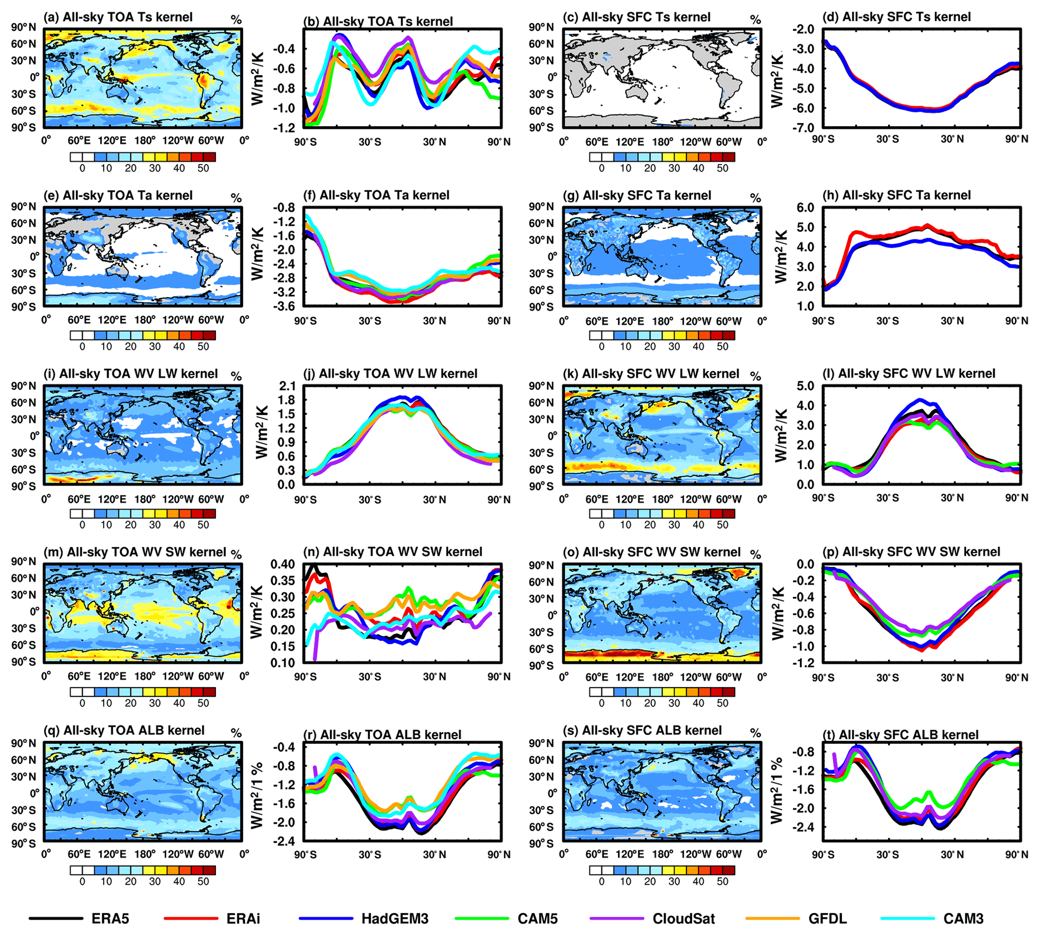
Figure 3 Contour plot: fractional discrepancies as measured by the normalized standard deviation of the kernels by Eq. (3); line plot: zonal mean distribution of multi-kernels in all sky.

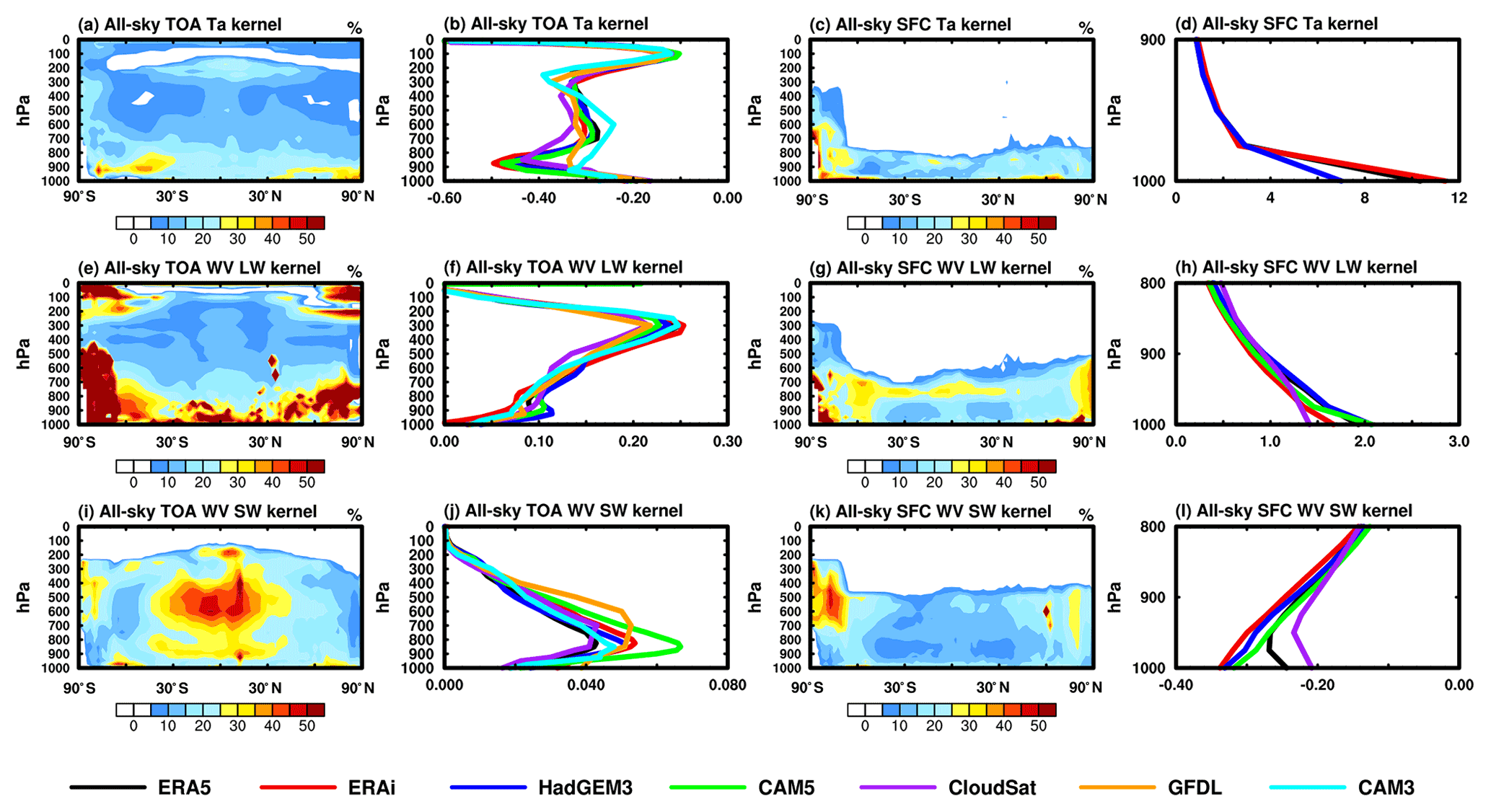
Figure 4 Contour plot: cross-section of fraction discrepancies of the radiative kernels; line plot: global mean vertically resolved kernels from multi-datasets in all sky.

Here we use the standard deviation (SD) and its normalized value (SD^∗) to measure the spread of the inter-kernel dataset differences:

$$\begin{array}{}\text{(2)}& {\displaystyle }{\mathrm{SD}}_X=\sqrt{{\displaystyle \frac{\mathrm{1}}{n-\mathrm{1}}}\sum _{i=\mathrm{1}}^n{\left(K_X^i-\stackrel{\mathrm{‾}}{K_X}\right)}^{\mathrm{2}}},\text{(3)}& {\displaystyle }{\mathrm{SD}}_X^{\ast }={\displaystyle \frac{{\mathrm{SD}}_X}{\stackrel{\mathrm{‾}}{K_X}}}\cdot \mathrm{100},\end{array}$$

where n is the total number of kernel datasets. $K_X^i$ is the radiative kernel of variable X from the ith dataset. $\stackrel{\mathrm{‾}}{K_X}$ is the multi-dataset mean of radiative kernel K_X. Note that $\stackrel{\mathrm{‾}}{K_X}$ does not represent the “truth” value but a reference value used to measure the spread of multi-kernel values. The vertically integrated and the vertically resolved but zonally averaged distributions of fractional discrepancy (SD^∗) are shown in Figs. 3 and 4, respectively. The zonal mean kernel values from respective multi-datasets are shown in line plots in Figs. 3 and 4. Note that some kernels exhibit abnormal values, such as the surface and air temperature kernel of the surface flux in the CAM5 and CloudSat kernels (see the Appendix Fig. A2), indicating inconsistent computation of their values, and thus are excluded in the corresponding ${\mathrm{SD}}_X^{\ast }$ statistics in Figs. 3 and 4. See more discussions in the Appendix.

The comparisons identify the following relatively larger differences in kernel values. Among the TOA kernels, the surface temperature and albedo kernels show relatively large discrepancies in the Arctic, Southern Ocean and over some continental regions in the tropics in all sky (Fig. 3a and q), with the maximum discrepancy exceeding 30 %. The air temperature kernel shows larger discrepancies in the lower troposphere and tropical tropopause region (Fig. 4a). These kernel differences are likely due to the differences in cloud fields. The water vapor LW kernel also shows noticeable fractional differences, for example, over the Antarctic region (Figs. 3i and 4e). The water vapor SW kernel shows differences in the tropical mid-troposphere and over the Antarctic in both clear sky and all sky (Figs. 4i and S6i), leading to strong variations in the vertical integration of sensitivity (Figs. 3m and S5m), with a spread exceeding 30 %. The noticeable periodic equatorial pattern in Fig. S5m is caused by the CAM3 kernel, likely due to a coarser temporal resolution that does not resolve the diurnal cycle of solar insolation in the kernel computation well.

For the surface kernels, the most prominent differences exist in SW radiative kernels (Figs. 3 and 4), especially in the polar regions. The discrepancy in the water vapor SW kernel reaches 30 % for vertically integrated values (Fig. 3o), with noticeable differences through the troposphere (Fig. 4k). The surface albedo kernel differences are much larger in all sky than that in clear sky (Figs. 3 and S5), indicating that the cause is in cloud fields, and are also noticeable in the Arctic region due to sea ice variations (Fig. 3s). In the LW, the water vapor kernels exhibit noticeable differences in the central Pacific, Southern Ocean and Arctic in all sky (Fig. 3k), where again the difference in cloud field is likely the cause. The air temperature kernels show noticeable discrepancies in the bottom layers (Fig. 4d), which may be caused by inconsistency in the kernel computation and vertical resolutions (see the discussions in the Appendix).

In summary, the differences among radiative kernel datasets are generally smaller in clear sky than in all sky and, in most cases, are within 10 % of the radiative kernel values. However, there are some notable regional discrepancies, for example, in the surface temperature kernel in the tropics (Fig. 3a), in the surface albedo kernel in the Arctic (Fig. 3q) and in the water vapor SW kernel in the Antarctic region (Fig. 3m). As different kernel datasets are calculated using different data sources, the discrepancies detected here are likely due to the state dependency in the kernels, which differs between the kernel datasets. To ascertain the state-dependency-caused kernel uncertainty, we next examine the ERA5 kernels computed from different years, i.e., from different atmospheric states, to investigate how much difference in radiative sensitivity can result from the change in atmospheric state.

3.3 Interannual variation in kernel values

The intercomparison above identified several prominent inter-dataset differences in the kernel values. For example, there are noticeable differences in the values of surface temperature, albedo and water vapor kernels in the central Pacific and Arctic regions. One possible reason that may account for such differences is the atmospheric state dependency of the kernel values. Besides the inter-model differences in the different GCM climatology, interannual variations in the atmospheric states, such as cloudiness variations in the central Pacific region during the ENSO cycle, may affect the radiative sensitivity as some radiative kernels are calculated using 1 arbitrary year's data. To test this hypothesis, we use the ENSO and sea ice loss cases to demonstrate the changes in radiative sensitivity with a focus on the central Pacific and Arctic regions, respectively. In the ENSO case, the variation is defined as the difference in annual mean kernel values between 2015 and the 5-year mean (from 2011 to 2015), which have annual mean sea surface temperature anomalies in the Niño 3.4 region (5^∘ N–5^∘ S, 190–240^∘ E) over +2.0 K. In the sea ice loss case, the variation is calculated as the difference in September between the years 2012 and 2013, as the sea ice cover in 2012 was reported to be the lowest level in the satellite observation era. In addition, we further show the comparison between ERA5 and ERAi kernels (in Fig. 5), which was also calculated by RRTMG and averaged from 5-year calculations (2008–2012), to compare the inter-kernel difference and interannual difference in kernel values.

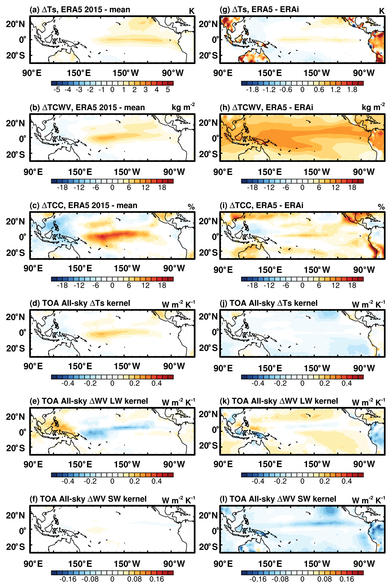
Figure 5 Differences in climate states and all-sky kernel values (left) between an arbitrary year (2015) and a 5-year mean of ERA5 and (right) between the 5-year means of ERA5 and ERAi datasets: (a, g) skin temperature, (b, h) total-column water vapor (TCWV), (c, i) total cloud cover (TCC), (d, j) TOA skin temperature kernel, (e, k) TOA vertically integrated water vapor LW kernel and (f, l) TOA vertically integrated water vapor SW kernel. Note that the color bar ranges differ among panels.

To save space, here we only highlight the most prominent differences. Figure 5a–c show the differences in skin temperature, total-column water vapor and total cloud cover due to ENSO, and Fig. 5d–f summarize the corresponding differences in all-sky TOA kernels. As the skin temperature in the central Pacific warms over 2 K (Fig. 5a) during ENSO, the increases in water vapor concentration and cloud fraction (Fig. 5b and c) reduce the sensitivity of TOA flux to surface temperature change by about 0.2 W m⁻² K⁻¹ (about 33 %) (Fig. 5d). The moistening in the central Pacific (Fig. 5b) enhances the TOA water vapor LW sensitivity in the clear sky (Fig. S7b), while in all sky the enhanced convection and associated total cloud cover in this region lead to a weakened TOA water vapor LW radiative sensitivity (Fig. 5e) despite the moist anomaly, and the decrease is contributed from almost the whole troposphere (Fig. S8c). The water vapor SW kernel discrepancy is less pronounced (Fig. 5f).

Comparing the 5-year averaged all-sky ERA5 and ERAi kernels, we find that the atmospheric state differences also exist between the atmospheric datasets on which the kernels are computed. For example, ERA5 shows similar, but less pronounced, warming anomalies in sea surface temperature in the central Pacific compared to ERAi, partly due to the strong El Niño year (2015) included in the ERA5 dataset. ERA5 data also show more water vapor and cloud cover (Fig. 5h and i). Although the total-column water vapor and total cloud cover are higher in ERA5 (Fig. 5h and i), their differences are complex and vertically non-uniform (Fig. S8d and e), which leads to a slight strengthening of surface temperature kernels compared with ERAi (Fig. 5j). It is also noticed that the ERA5 water vapor SW kernel shows lower sensitivity (Fig. 5l), which mainly comes from the contributions in the mid- to low troposphere (Fig. S8f). The difference noticed in Fig. S8f corresponds to the discrepancy noticed in Fig. 4i, which are both in the mid- to low troposphere, and the corresponding clear sky have far fewer differences (Fig. S7), suggesting that the difference in clouds might be the main cause of the all-sky kernel differences, which also correspond to the discrepancies shown in the multi-kernel comparisons in Fig. 3a, i, and m.

In the sea ice loss case, the reduction in sea ice in the Arctic region (Fig. 6a) leads to a significant decrease in radiative sensitivity to surface albedo in the areas with noticeable sea ice retreats (Fig. 6d and f), with the maximum difference exceeding 30 % of the radiative kernel value, because of the nonlinear dependency of the reflected solar radiation on the surface albedo (e.g., see Y. Huang et al., 2021, Figs. 3 and 6). The cloud cover changes also contribute to changes in surface albedo kernel values due to the coupling effect between cloud and surface albedo (see Y. Huang et al., 2021), which for example is seen in Siberia and the western coastline of Europe. The change in sea ice also leads to a significant decrease in the TOA sensitivity and an increase in surface sensitivity to water vapor in the sea ice loss region (Fig. 6c and e), with the maximum changes exceeding 80 % for the surface. All these results confirm the state dependency of radiative kernels (e.g., Riihelä et al., 2021).

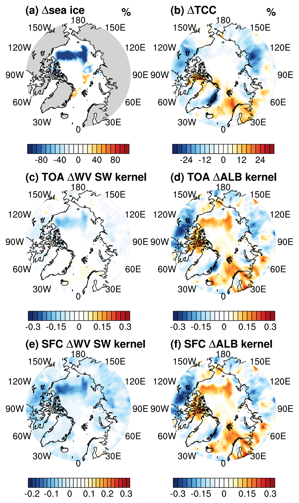
Figure 6 September differences between 2012 and 2013 in (a) sea ice concentration, (b) total cloud cover (TCC), and the differences in (c, e) water vapor SW kernels for TOA and surface fluxes (units: W m⁻² K⁻¹) and (d, f) surface albedo kernels for TOA and surface fluxes (units: W m⁻² 1 %⁻¹). Note that the color bar ranges differ among panels.

In summary, these quantitatively large interannual differences, as well as their locations, verify that some discrepancies between the radiative kernels are caused by the difference in atmospheric states and partly explain the inter-dataset kernel differences seen in Figs. 3 and 4. Nevertheless, it ought to be noted that the differences are localized and because of that do not cause significant differences in the global mean feedback values (see Sect. 4). The results above also show that kernel values based on 1 arbitrary year may be regionally different. If only 1 year's atmospheric profiles are used to generate radiative kernels, we recommend selecting a year without significant anomalies in atmospheric states, e.g., due to El Niño or severe sea ice loss, so that the computed kernel values better represent the radiative sensitivity climatology.

4 Feedback quantification

In this section, we apply different kernels to quantifying the radiative feedbacks in one quadrupling CO₂ experiment (abrupt4xCO₂) of CMIP6 models. This experiment is selected because it has been used by a number of studies for forcing and feedback analyses (e.g., Zelinka et al., 2020), which we can compare our results to. The CMIP6 models used in this assessment are listed in Table 2. Note that the standard outputs at 19 pressure levels from the models and correspondingly the kernel values, including CAM5 and HadGEM3, provided at the pressure levels are used in this section.

Table 2 Summary of CMIP6 models used in this study.

4.1 Analysis procedure

To quantify the radiative feedbacks, data from two experiments as documented by Eyring et al. (2016) and Pincus et al. (2016) are used: abrupt4xCO₂ simulations with an instantaneous quadrupling of CO₂ concentration of the year 1850 and piClim-4xCO₂ simulations with sea surface temperature (SST) and sea ice concentrations fixed at the climatology of a pre-industrial control experiment and the CO₂ concentration quadrupled. In each experiment, a 20-year period at the end of the simulation in each model is used. For example, in the models where the abrupt4xCO₂ simulation is longer than 150 years, the simulations from the last 20 years rather than those from years 131 to 150 are used for the calculation. To exclude the effect of rapid adjustments, the radiative feedbacks in this study are measured using the difference in feedback variables between the abrupt4xCO₂ and piClim-4xCO₂ experiments and vertically integrated from the surface to the model top. Note that these treatments are different from some other studies, e.g., Zelinka et al. (2020), which used the piControl (pre-industrial control) simulation as the climatology baseline and vertical integration from the surface to the tropopause, although the quantitative differences in the diagnosed global mean feedback values are small.

To detail the analysis procedure, firstly, all variables including radiative fluxes and atmospheric variables from CMIP6 models are interpolated to the horizontal and vertical resolution of the kernel itself. Note that for CAM3, GFDL, CloudSat and CAM5 kernels, they only have 17 pressure levels, which is two layers (1 and 5 hPa) fewer than the CMIP6 standard model output. To address this issue, the contribution of the two missing layers is calculated using other kernels (e.g., ERA5) and found to have a negligible effect on the global mean feedback value. Hence, when using these three kernels, the contributions from 10 hPa above are ignored.

Secondly, the non-cloud radiative feedback of variable X (ΔR_X) is calculated as

$$\begin{array}{}\text{(4)}& \mathrm{\Delta }{R}_X=K_X\cdot \mathrm{\Delta }X,\end{array}$$

with units in W m⁻², where K_X is the monthly mean radiative kernel of variable X and ΔX is the monthly mean anomaly of X measured by the difference between abrupt4xCO₂ and piClim-4xCO₂ and represents the anomalies of surface temperature (ΔT_s), air temperature (ΔT_a), water vapor (ΔWV) and surface albedo (ΔALB). For the 2D radiative kernels (surface temperature and surface albedo), K_X and ΔX have just single layer values and ΔR_X is simply the product of these two terms. For the 3D radiative kernels (air temperature and water vapor), both K_X and ΔX are vectors of pressure levels and ΔR_X is the dot product of K_X and ΔX and is integrated from TOA to 1000 hPa. Note that if K_X is normalized with unit pressure thickness (e.g., W m⁻² K⁻¹ 100 hPa⁻¹), the layer thickness must be taken into account when calculating dR_X. See the Appendix for further discussion on the application of thickness-weighted kernels.

Finally, cloud feedbacks are diagnosed using the adjusted cloud-radiative forcing method (Shell et al., 2008). Here we compute the residual term in clear sky as

$$\begin{array}{}\text{(5)}& {\mathrm{res}}^o=\mathrm{\Delta }{R}^o-\sum \mathrm{\Delta }{R}_X^o,\end{array}$$

which represents the unexplained part of radiation budget change, and, assuming the all-sky decomposition has the same non-closure residual, the cloud feedback is measured as

$$\begin{array}{}\text{(6)}& \mathrm{\Delta }{R}_{\mathrm{C}}=\mathrm{\Delta }R-\sum \mathrm{\Delta }{R}_X-{\mathrm{res}}^o,\end{array}$$

where the superscript o represents clear-sky quantities. $\sum \mathrm{\Delta }{R}_X^o$ and ∑ΔR_X are the sum of non-cloud feedbacks in clear sky and all sky, respectively, diagnosed by multiplying the radiative kernel with the atmospheric responses measured as the difference between abrupt4xCO₂ and piClim-4xCO₂ experiments. ΔR^o and ΔR are the total radiation change in clear sky and all sky, respectively, calculated as the difference in the GCM-simulated radiative fluxes between two experiments. It is worth noting that ΔR_C measured according to Eq. (6) is essentially the part of total radiation change not explained by the non-cloud feedbacks and is equivalent to the other formulations of the adjusted cloud radiative effect method (e.g., Soden et al., 2008; Huang, 2013). Interested readers can refer to, for example, Huang (2013) for a detailed formulation and explanations of the method.

The feedback parameters, λ_X, in the units of W m⁻² K⁻¹, are then obtained by normalizing the feedback flux changes ΔR_X by the global mean surface temperature change ΔT_S in the abrupt4xCO₂ experiment:

$$\begin{array}{}\text{(7)}& {\mathit{\lambda }}_X=\mathrm{\Delta }{R}_X/\mathrm{\Delta }{T}_{\mathrm{S}}.\end{array}$$

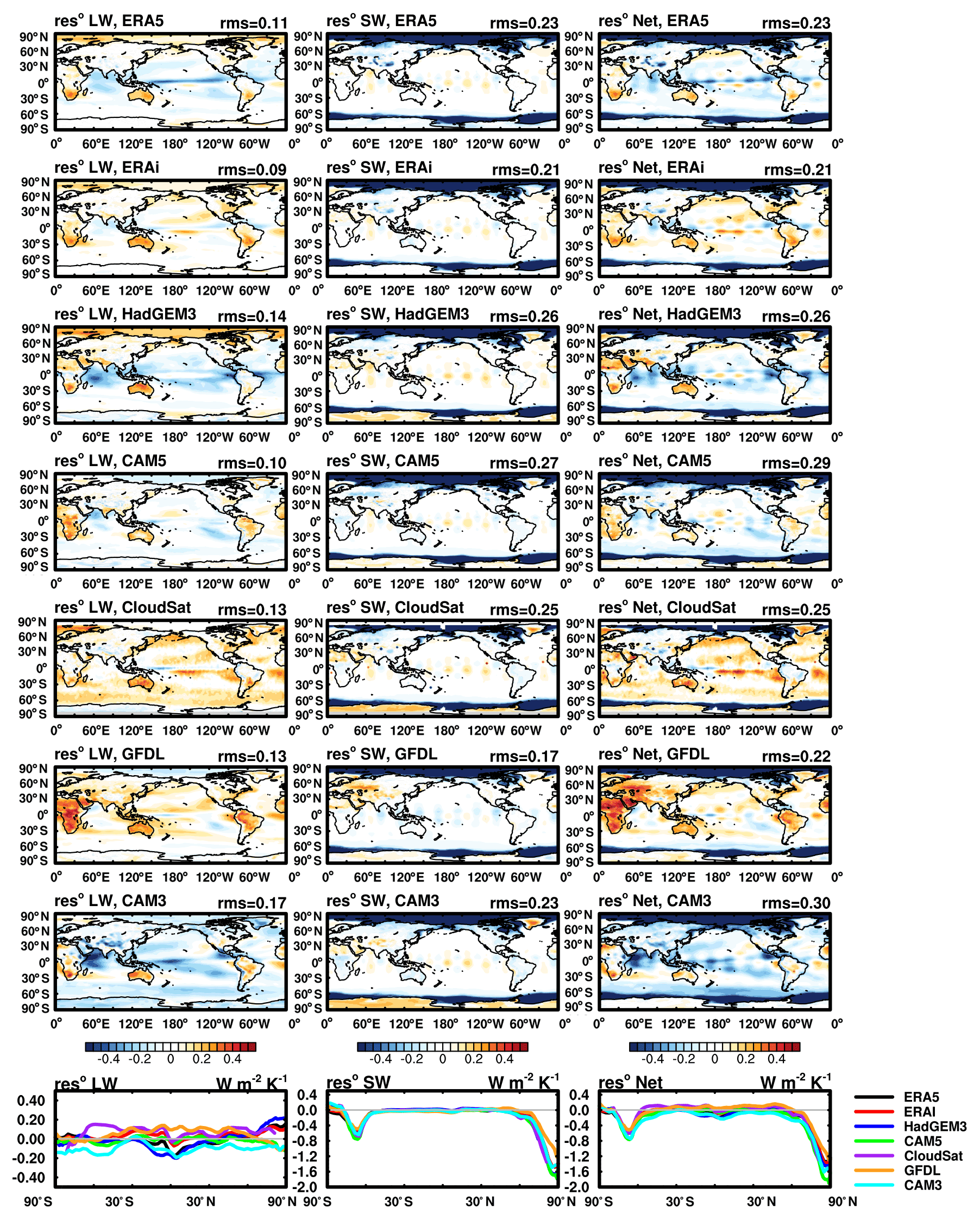
Figure 7 The residuals (res^o) in the multi-model mean TOA feedback decomposition when different kernels are used: LW (left column); SW (middle column); net (right column), the sum of LW and SW. The three line plots in the bottom row are the zonal mean residuals. Numbers in the right corner in each panel are the spatial root-mean-square values.

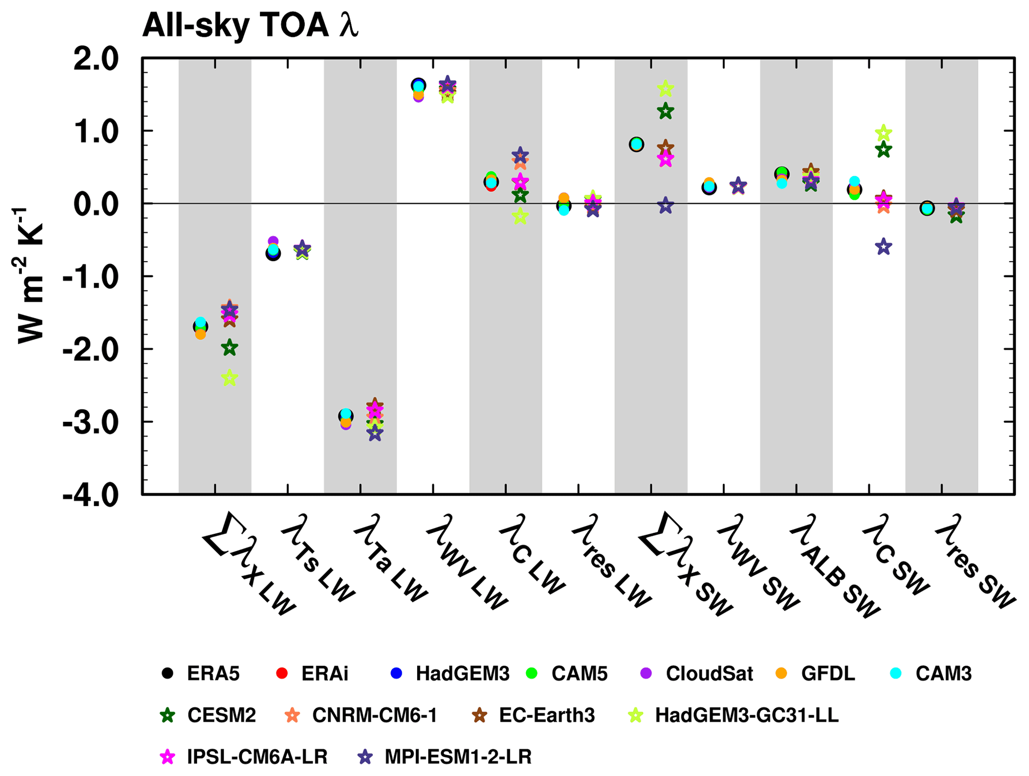
Figure 8 Global mean TOA feedback parameters in all sky diagnosed by the kernels listed in Table 1 across CMIP6 models. Dot marks represent multi-model mean values computed from different kernel datasets. Stars represent the multi-kernel mean results computed from different GCMs.

4.2 TOA feedbacks

The residual term (res^o) measures the unexplained radiation change in the feedback analysis and provides a useful overall indication of the soundness of the feedback quantification. Figure 7 illustrates the residual term for the TOA flux decomposition when different kernels are used to diagnose the multi-model mean feedbacks. In terms of the global mean, all residual terms are of small magnitude, no matter which kernel dataset is used (Fig. 8 and Table S1). However, there are some noticeable local residuals, especially for the SW budget, e.g., in the Arctic region and around the Antarctic continent where sea ice changes the most (middle column in Fig. 7). While the non-zero magnitude of the residual is partly due to nonlinearity in the radiation decomposition, e.g., possible coupling between surface albedo and water vapor (Y. Huang et al., 2021), the spread among the kernel results as evidenced by the line plots of Fig. 7 is attributable to the discrepancies in the SW radiative kernels as revealed by the comparisons in Sect. 3. In the LW, the residual is generally small compared with the total feedback. In summary, the residual terms for the TOA budget are small in terms of the global mean feedback strengths, confirming the validity of the radiative kernels for feedback quantification. Here, we use the spatial root-mean square (rms) of the residuals to quantify the regional biases, which are shown by the numbers in the right corner of each panel in Fig. 7. For LW, results from ERA5, ERAi and CAM5 kernels show relatively smaller regional biases compared to those from HadGM3, CloudSat and CAM3 kernels. For SW, all kernel datasets have similar regional non-closures, for example, in the polar regions (Figs. 7 and 8). This is largely caused by the nonlinearity in albedo feedback and also the coupling effect between water vapor and surface albedo feedbacks (Y. Huang et al., 2021; Block and Mauritsen, 2013). In summary, these results suggest that for the TOA feedback quantification, the performance of the ERA5 kernel is comparable to the other datasets.

Figure 8 compares the spreads of feedback values resulting from the differences in kernels and those from the different projections of GCMs. In general, feedbacks from different kernel datasets overlap each other, even for cloud feedbacks, indicating a good consistency between the results computed from different kernel datasets. However, the spread across the GCMs is considerably larger, suggesting the overall feedback uncertainty is dominated by inter-model spread rather than the kernel uncertainty. The values of the feedbacks from each model and kernel datasets are shown in Tables S1 and S2 for readers who are interested. These results are consistent with other published results. For example, compared with the results of Zelinka et al. (2020) based on the ERAi kernel, the kernel-diagnosed overall feedback parameter in the two results is −0.87 and −0.85 W m⁻² K⁻¹ for the CNRM-CM6-1 model and −0.81 and −0.84 W m⁻² K⁻¹ for the HadGEM3-GC3-LL model.

In summary, in terms of TOA feedback values, the inter-kernel differences lead to a small uncertainty in the analyzed non-cloud feedbacks; the kernel-induced uncertainty in cloud feedback is relatively larger (Table S2), with the inter-kernel spread in cloud LW feedback coming almost equally from the spread in surface and air temperature feedback and water vapor LW feedback (as measured by the $\sum \mathrm{\Delta }{R}_X^o-\sum \mathrm{\Delta }{R}_X$ terms in Eq. 6) and the inter-kernel spread in cloud SW feedback coming more from the spread in surface albedo feedback than from water vapor SW feedback (not shown). Despite this, this uncertainty is considerably less than the inter-GCM cloud feedback spread.

4.3 Surface feedbacks

Next, we examine how the inter-kernel differences lead to uncertainty in the analyzed surface feedbacks.

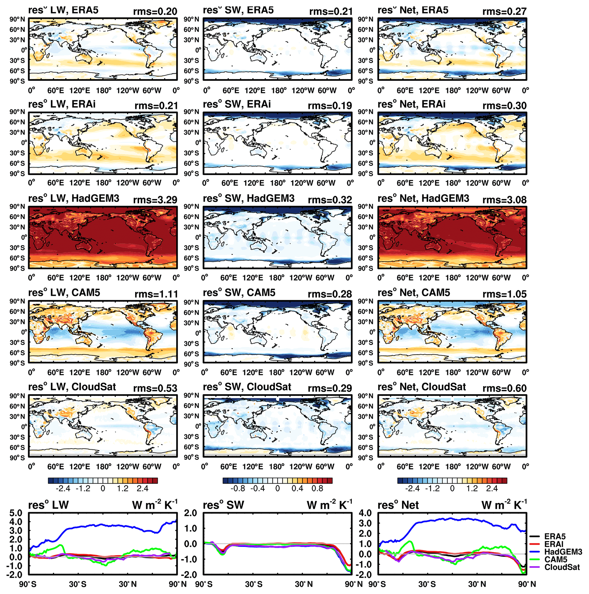
Figure 9 Similar to Fig. 7 but for the surface feedback analysis.

Figure 10 Similar to Fig. 8 but for the surface feedback parameter.

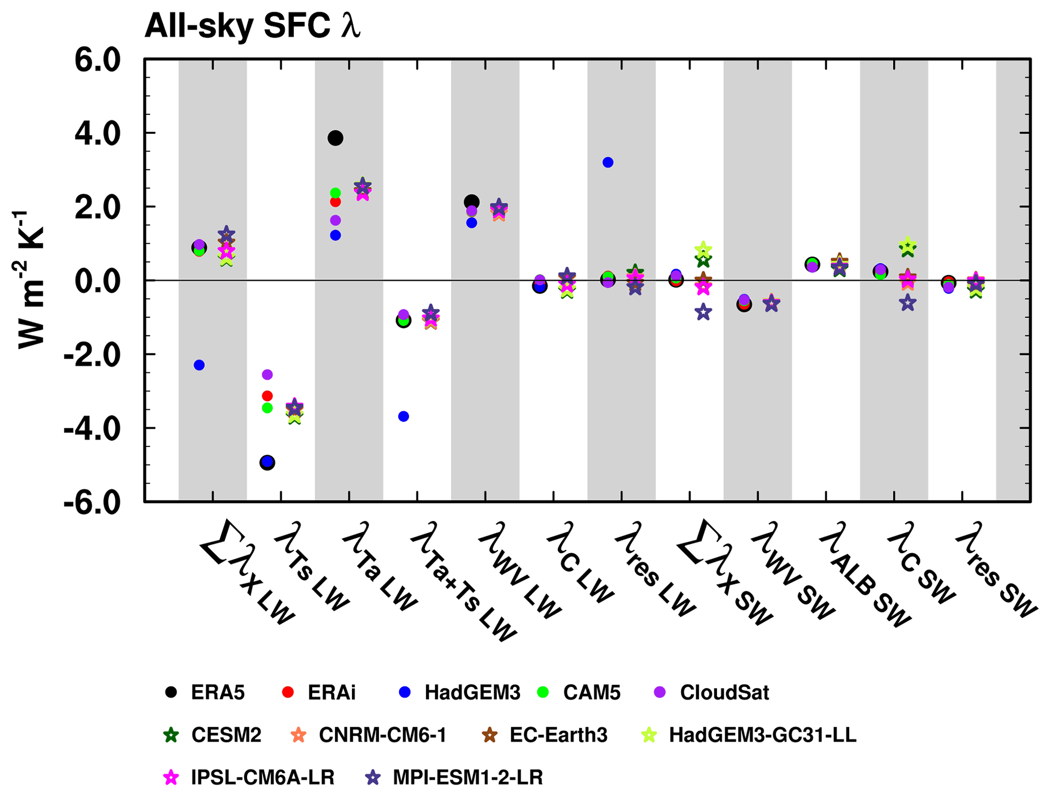
Figure 9 shows the residual distribution. We find that when the ERA5 and ERAi kernels are used for the feedback analysis, the non-closure residual in the surface budget is comparable in magnitude to the TOA analysis. This suggests that the surface kernels afford a valid tool for the surface feedback analysis. However, some prominent biases are noticed for other kernel datasets. For example, the HadGEM3 kernels particularly show an underestimation in air temperature feedback, likely due to a biased sensitivity of the bottom atmospheric layer (see the Appendix for more discussions). The sum of global mean surface and air temperature feedback parameters measured by the HadGEM3 kernel is around −3.70 W m⁻² K⁻¹ (Table S4, compared to around −1.0 W m⁻² K⁻¹ measured by the other kernels), and the non-closure residual is as large as 3.0 W m⁻² K⁻¹ (Table S3, compared to −0.1 W m⁻² K⁻¹ in the others). For this reason, the result from the HadGEM3 kernel is excluded for the multi-kernel statistics in Fig. 10, Table S3 and S4 but listed in a separate row for comparison. From either the spatial distribution of residual terms or the spatial rms residuals, the ERA5 kernel and ERAi kernel show a superior performance than the other datasets. The use of ERA5 kernels may be advantageous for diagnosing the surface radiation budget, considering that ERA5 data are a newer-version reanalysis dataset from ECMWF compared with ERAi, and their quality has been widely validated.

Figure 10 compares the inter-model and inter-kernel spreads for the surface feedbacks. Unlike the results for TOA, the inter-kernel spread can be as large as the inter-model spread, for example, in LW surface temperature feedback, air temperature feedback and water vapor feedback. The sum of air temperature and surface temperature feedbacks shows better consistency compared with the respective components (except for the HadGEM3 kernel), and the respective air temperature and surface temperature feedbacks quantified by the ERA5 kernel are stronger than the results from the other kernels. These discrepancies are due to the reason discussed in the Appendix – a possibly wrong quantification of surface temperature effect. In SW, the multi-kernel results are close to each other, showing smaller inter-kernel spreads than the inter-model spreads.

In summary, we find the surface feedback decomposition can achieve a similar level of radiation closure to the TOA analysis when using ERA5 kernels, confirming the validity of kernels for diagnosing the surface radiative feedback. However, the results qualitatively vary depending on which kernel dataset is used, indicating errors in the computation of some kernels.

5 Data availability

The datasets containing the multi-year averaged monthly mean TOA and surface kernels for surface temperature, air temperature, surface albedo and water vapor (LW and SW) are available at https://doi.org/10.17632/vmg3s67568 (Huang and Huang, 2023). Other kernel datasets used in this study, interpolated to the same horizontal and vertical grids as the ERA5 kernels, are also provided at this link.

6 Conclusions and discussions

In this paper, we present a newly generated set of ERA5-based radiative kernels of surface and air temperatures, water vapor, and surface albedo, for both TOA and surface radiation fluxes. We also compare them with other published kernels, including the kernel-diagnosed radiative feedbacks for both the TOA and surface radiation budgets.

For the TOA kernels, the results here demonstrate general consistency among the different kernel datasets, and the discrepancies are generally within 10 % in terms of vertically integrated or globally averaged radiative sensitivity, although some relatively larger regional differences are noticed, including those in the surface temperature kernel in the tropics (Fig. 3a), those in the surface albedo kernel in the Arctic (Fig. 3q) and those in the water vapor shortwave kernel over Antarctica (Fig. 3m), which is partly due to the dependence of radiative sensitivity on background climate states.

For the surface kernels, more prominent inter-kernel differences are found. For example, the differences in the water vapor shortwave kernel in the Antarctic (Fig. 3o) and in the surface albedo kernel in the Arctic (Fig. 3s) can reach 30 % of the kernel value itself. Some kernels have considerably biased air temperature sensitivity values in the bottom atmospheric layers, which is likely due to improper treatment in the perturbation experiments used for kernel computation (see the Appendix). The differences in both TOA and surface kernels discovered here emphasize the importance of validating the radiative sensitivity as noted by Huang and Wang (2019) and Pincus et al. (2020).

The investigation of interannual variability in ERA5 kernels validates the dependence of radiative sensitivity on atmospheric state and the further comparison between ERAi and ERA5 kernels (Fig. 5) reveals the effects of clouds on the kernel values, which might explain the discrepancies between multi-kernel datasets (Fig. 3).

Applying the different kernels to quantifying the TOA and surface radiative feedbacks, we find that for TOA feedback quantification, the ERA5 kernels are as accurate as other kernel datasets, while for surface feedback, ERA5 and ERAi kernels show superior accuracy compared with other datasets. Considering the strengths of the ERA5 dataset in representing the atmospheric states, we recommend the use of ERA5 kernels.

In addition, we compare the feedback differences caused by using different kernels and also the inter-GCM spread of the feedback values (when measured by the same kernel). We find the kernel difference is not a major cause of the inter-GCM TOA feedback spread (Figs. 7 and 8). This finding is consistent with the previous assessments (e.g., Soden et al., 2008; Jonko et al., 2012; Vial et al., 2013).

Radiation closure tests show that the unexplained residuals are generally within 10 % of the total feedback for both TOA and surface analyses in terms of the global mean feedback, confirming the validity of the kernels for feedback quantification for both budgets. This suggests that the large non-closure residuals reported in some previous studies (e.g., Vargas Zeppetello et al., 2019) are likely due to kernel inaccuracy rather than the limitation of the kernel method. However, there are more significant local non-closures, for example, in the shortwave in the Arctic region and around the Antarctic continent, which is contributed, but cannot be fully explained, by the kernel uncertainty. This points to the accuracy limit of the kernel (linear) method and calls for more advanced methods, such as the neural network method (Zhu et al., 2019), for local feedback analysis.

Appendix A

The ERA5 kernels are computed following Eq. (1) and the approach outlined in Sect. 2.2.

A1 Surface variable kernels

To execute the partial radiative perturbation computations, the perturbations are prescribed as the following: for the 2D feedback variables, the surface temperature is increased by 1 K and the albedo is increased by 0.01 at each location. Hence, the units of the two kernels, $K_{T_{\mathrm{s}}}$ and K_ALB are W m⁻² K⁻¹ and W m⁻² %⁻¹, respectively. When applying them to feedback quantification, their feedbacks are quantified as

$$\begin{array}{}\text{(A1)}& {\displaystyle }\mathrm{\Delta }{R}_{T_{\mathrm{s}}}=K_{T_{\mathrm{s}}}\cdot \mathrm{\Delta }{T}_{\mathrm{S}},\text{(A2)}& {\displaystyle }\mathrm{\Delta }{R}_{\mathrm{ALB}}=K_{\mathrm{ALB}}\cdot \mathrm{\Delta }\mathrm{ALB},\end{array}$$

where ΔT_S should be measured in the units of K and ΔALB in absolute values divided by 1 %.

A2 Water vapor kernel

For the 3D feedback variables, the perturbations are applied to each of the 37 pressure layers (from 1 to 1000 hPa) and one layer at a time. For the water vapor kernel, a 10 % incremental perturbation of the water vapor concentration is used. To adapt to the convention used in the majority of the existing kernels, we convert the units of the kernels to represent the radiative flux change corresponding to an increase in water vapor concentration that conserves the relative humidity of the layer under a 1 K increase in air temperature, i.e., converting the units from W (m² $\mathrm{\Delta }{q}_{\mathrm{0}}^{+\mathrm{10}\mathit{\%}}$ 100 hPa)⁻¹ to W (m${}^{\mathrm{2}}\mathrm{\Delta }{q}_{\mathrm{0}}^{+\mathrm{1}\mathrm{K}}$ 100 hPa)⁻¹:

$$\begin{array}{}\text{(A3)}& {\displaystyle }{K}_q^{+\mathrm{10}\mathit{\%}}={\displaystyle \frac{\mathrm{\Delta }{R}_{\mathrm{0}}}{\mathrm{\Delta }{q}_{\mathrm{0}}^{+\mathrm{10}\mathit{\%}}}},\text{(A4)}& {\displaystyle }\begin{array}{rl}{K}_q^{+\mathrm{1}\mathrm{K}}& ={\displaystyle \frac{\mathrm{\Delta }{R}_{\mathrm{0}}}{\mathrm{\Delta }{q}_{\mathrm{0}}^{+\mathrm{1}\mathrm{K}}}}=K_q^{+\mathrm{10}\mathit{\%}}\cdot {\displaystyle \frac{\mathrm{\Delta }{q}_{\mathrm{0}}^{+\mathrm{10}\mathit{\%}}}{\mathrm{\Delta }{q}_{\mathrm{0}}^{+\mathrm{1}\mathrm{K}}}}\\ & =K_q^{+\mathrm{10}\mathit{\%}}\cdot {\displaystyle \frac{\mathrm{\Delta }{q}_{\mathrm{0}}^{+\mathrm{10}\mathit{\%}}}{q_{\mathrm{0}}}}\cdot {\displaystyle \frac{e_{\mathrm{s}}\left(T_{\mathrm{0}}\right)}{e_{\mathrm{s}}\left(T_{\mathrm{0}}+\mathrm{1}\mathrm{K}\right)-e_{\mathrm{s}}\left(T_{\mathrm{0}}\right)}},\end{array}\end{array}$$

where q₀ is the unperturbed water vapor concentration in units of kg kg⁻¹. $\mathrm{\Delta }{q}_{\mathrm{0}}^{+\mathrm{10}\mathit{\%}}$ is a 10 % increment in water vapor concentration. e_s(T) is the saturated water vapor pressure under temperature T and can be measured by empirical formulas; hence, $\mathrm{\Delta }{q}_{\mathrm{0}}^{+\mathrm{1}\mathrm{K}}$ can be measured as $q_{\mathrm{0}}[\frac{e_{\mathrm{s}}\left(T_{\mathrm{0}}+\mathrm{1}\mathrm{K}\right)}{e_{\mathrm{s}}\left(T_{\mathrm{0}}\right)}-\mathrm{1}]$. Accordingly, when the water vapor kernel is used for water vapor feedback quantification, the feedback is measured as

$$\begin{array}{}\text{(A5)}& \begin{array}{rl}\mathrm{\Delta }{R}_q& =K_q^{+\mathrm{1}\mathrm{K}}\cdot \mathrm{\Delta }{q}^{+\mathrm{1}\mathrm{K}}=K_q^{+\mathrm{1}\mathrm{K}}\cdot {\displaystyle \frac{\mathrm{\Delta }q}{\mathrm{\Delta }{q}_{\mathrm{0}}^{+\mathrm{1}\mathrm{K}}}}\\ & =K_q^{+\mathrm{1}\mathrm{K}}\cdot {\displaystyle \frac{\mathrm{\Delta }q}{q_{\mathrm{0}}}}\cdot {\displaystyle \frac{e_{\mathrm{s}}\left(T_{\mathrm{0}}\right)}{e_{\mathrm{s}}\left(T_{\mathrm{0}}+\mathrm{1}\mathrm{K}\right)-e_{\mathrm{s}}\left(T_{\mathrm{0}}\right)}},\end{array}\end{array}$$

where $\mathrm{\Delta }q=q-q_{\mathrm{0}}$ measures the change in water vapor concentration and is normalized by $\mathrm{\Delta }{q}_{\mathrm{0}}^{+\mathrm{1}\mathrm{K}}$ to give the factor that is multipliable with the $K_q^{+\mathrm{1}\mathrm{K}}$ kernel value. If using the Clapeyron–Clausius relation, the above expression can be further approximated as

$$\begin{array}{}\text{(A6)}& \begin{array}{rl}\mathrm{\Delta }{R}_q& =K_q^{+\mathrm{1}\mathrm{K}}\cdot {\displaystyle \frac{\mathrm{\Delta }q}{q_{\mathrm{0}}}}\cdot {\displaystyle \frac{e_{\mathrm{s}}}{(\mathrm{d}{e}_{\mathrm{s}}/\mathrm{d}T)\cdot \mathrm{1}\mathrm{K}}}\\ & =K_q^{+\mathrm{1}\mathrm{K}}\cdot {\displaystyle \frac{\mathrm{\Delta }q}{q_{\mathrm{0}}}}\cdot {\displaystyle \frac{R_{\mathrm{v}}}{L_{\mathrm{v}}}}\cdot {\displaystyle \frac{T_{\mathrm{0}}^{\mathrm{2}}}{\mathrm{1}K}},\end{array}\end{array}$$

where R_v and L_v are the gas constant and specific latent heat of water vapor, respectively. Note that when the kernels are used, T₀ and q₀ typically take their values from the base climate appropriate to the application, e.g., the unperturbed climate of a GCM experiment, not necessarily the dataset used for kernel computation.

A3 Air temperature kernel

For the air temperature kernel, to be consistent with the “inhomogeneous path treatment” that accounts for the vertically non-uniform temperature distribution within each discrete atmospheric layer (Mlawer et al., 1997), perturbations are added not only to the layer-mean temperature but also to the temperature at the exiting boundary of radiative fluxes of interest (i.e., the upper boundary of each layer for the TOA flux and the lower boundary for the surface flux) to appropriately represent the physical temperature perturbation in each layer.

A meaningful test to validate the validity of the air temperature kernel is a vertical sum test, i.e., a linear additivity test to verify the vertical integration of the kernel values reproducing the flux change, either at TOA or the surface, in response to a whole-column air temperature increase of 1 K. Figure A1 shows that the ERA5 kernel passes this test well. However, as shown by Fig. 9, some kernels (e.g., HadGEM3 kernel) show a much weaker radiative response at the surface, possibly due to improper treatment of the air temperature perturbation in the kernel computation, which may lead to an underestimated air temperature feedback and large biases in the surface feedback analysis.

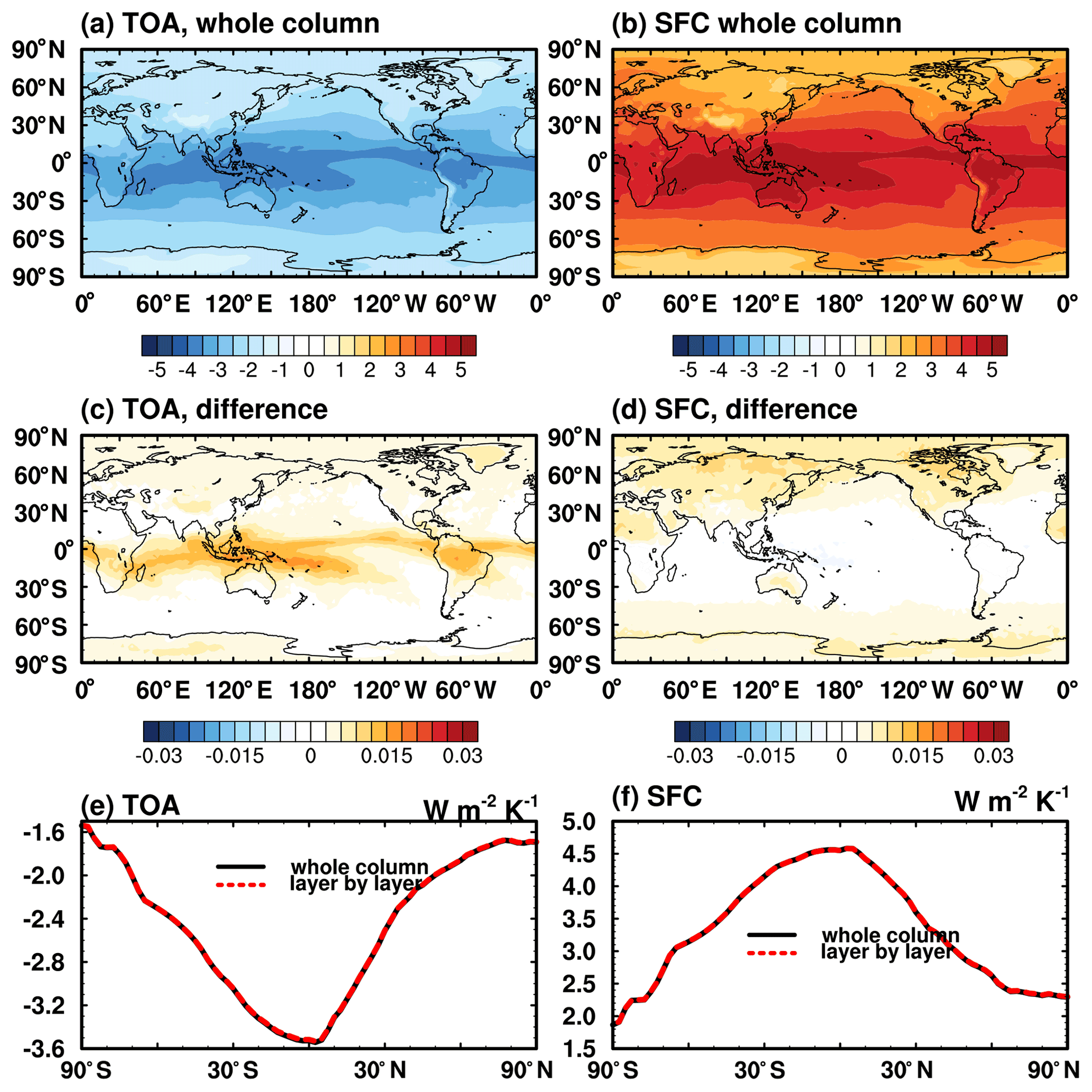
Figure A1 Monthly mean TOA and surface radiation flux change in response to a +1 K air temperature perturbation throughout the vertical column: (a, b) computed by a radiation model, RRTMG; (c, d) difference in the vertical sum of air temperature kernels compared to truth in (a), (b); (e, f) comparison of the zonal mean.

Another challenge in the computation of air temperature kernels for surface flux is that the surface in radiative transfer models is also the lower boundary of the lowermost atmospheric layer. If the effects of the surface temperature perturbation on the emission of the surface and that of the lowermost atmospheric layer are not distinguished, this may lead to improper interpretation and use of the surface temperature kernel. In our ERA5 kernel, the two effects are considered separately: according to radiative transfer theory, an increase in surface skin temperature only affects the surface upward emission; an increase in air temperature only affects the downward radiation. In some other kernels such as CAM5, these effects are not distinguished, so that the kernel value represents the net effect, i.e., a change in the sum of both downward and upward fluxes. As a result, in Fig. 10, we see stronger air temperature and surface temperature feedbacks quantified from ERA5 kernels than from other kernels, and in Table S4, we can only report the sum of surface and air temperature feedbacks.

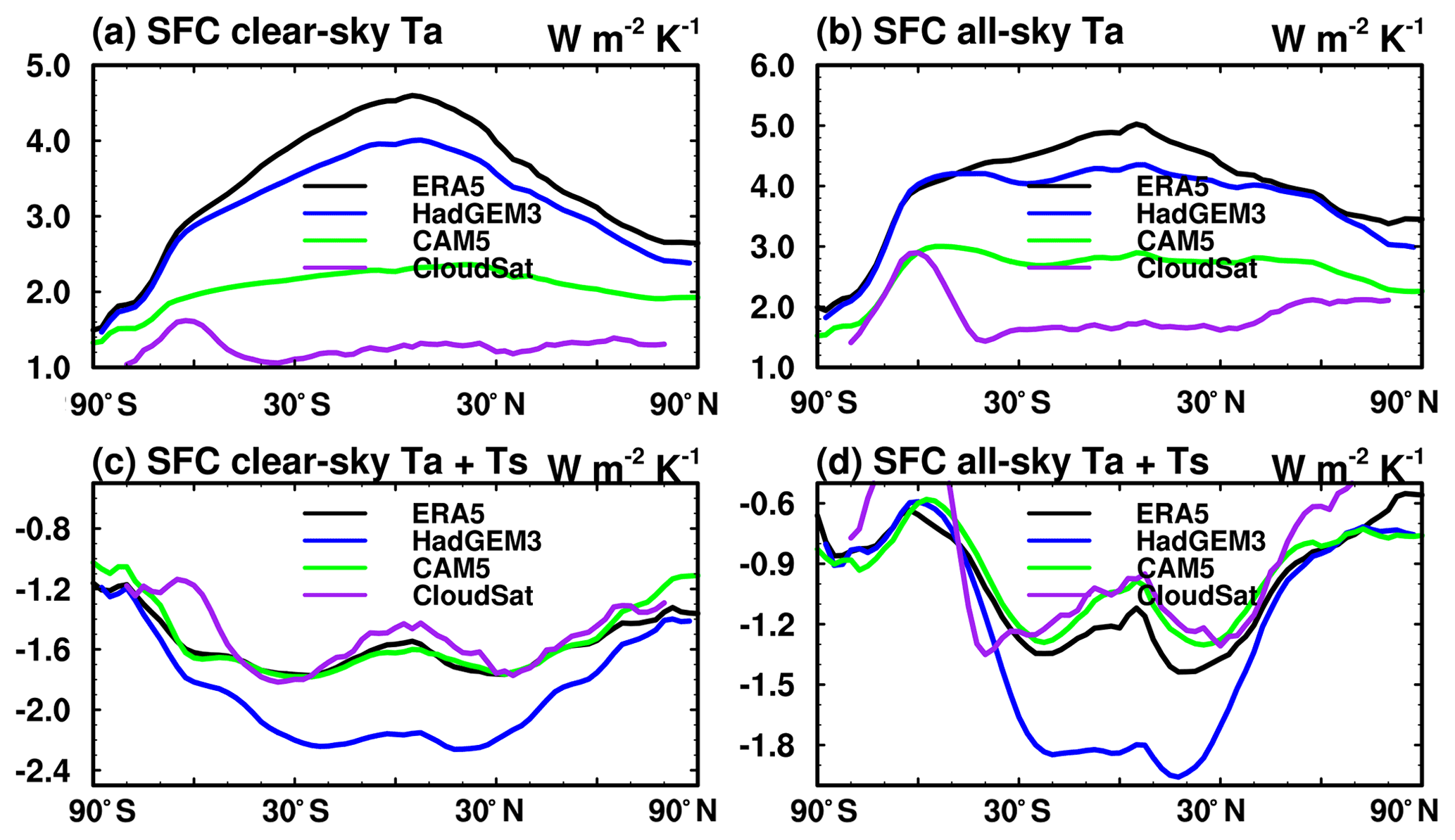
Figure A2 Comparison of annual mean surface kernels for ERA5, CAM5, CloudSat and HadGEM3 for (a, b) the vertically integrated air temperature kernel values and (c, d) sum of surface and air temperature kernels.

Figure A2 shows the comparison of vertically integrated air temperature kernels and the sum of surface and air temperature kernels between ERA5, CAM5, HadGEM3 and CloudSat. Although the strength of the vertically integrated air temperature kernel for CAM5 is much weaker than that for ERA5 (Fig. A2a and b), the sum of surface and air temperature kernels between these two datasets is in good agreement (Fig. A2c and d), which warns us that the seemingly right temperature feedback quantified by some kernels might come from the misattribution of surface temperature contributions. Another noticeable feature in Fig. A2 is that the HadGEM3 kernel shows an underestimation in the vertical integration of the air temperature kernel and an overestimation in the sum of surface and air temperature kernels, likely due to mistreatment of the bottom layer, and this accounts for the biased surface feedback analysis as shown in Fig. 9. Similar issues were noticed in Kramer et al. (2019a).

A4 Time averaging

As described in Sect. 2.2, all the kernels provided for feedback analysis are averaged from instantaneous kernel values over each calendar month and, in the ERA5 kernel, over multiple years. This is to ensure proper sampling of radiative sensitivity values under different atmospheric states, so that the kernels are representative of mean radiative sensitivity and thus can be readily multiplied with monthly mean climate responses (ΔX) to evaluate climate feedbacks.

If the kernels are computed for fixed pressure levels, and if the pressure of any of these levels of an instantaneous atmospheric profile is higher than the surface pressure (i.e., the level is below the surface) at a time instance, this potentially creates inconsistency in the averaging procedure. To address this concern, we set the kernel value to 0 (as opposed to a missing value) before averaging. This is to ensure that when multiplied with the monthly mean climate response (ΔX), the contribution of a pressure layer (e.g., that centered at 1000 hPa) is effectively counted only for the fraction of time the layer exists (when surface pressure is higher than 1000 hPa). Otherwise, the feedback quantification needs to be further weighted with the fraction of time (f) when the pressure layer exists. For example, if the surface pressure is larger than 1000 hPa only for half of the time in a month (f=0.5), the radiation flux anomaly contributed by the layer centered at 1000 hPa is

$$\begin{array}{}\text{(A7)}& \mathrm{\Delta }{R}_{T_{\text{1000\hspace{0.17em}hPa}}}=K_{T_{\text{1000\hspace{0.17em}hPa}}}^{\ast }\cdot \mathrm{\Delta }{T}_{\text{1000\hspace{0.17em}hPa}}\cdot f.\end{array}$$

Here, $K_{T_{\text{1000\hspace{0.17em}hPa}}}^{\ast }$ represents the kernel value averaged from the time instances when the layer exists. Our averaging scheme is essentially to provide a kernel $K_{T_{\text{1000\hspace{0.17em}hPa}}}=K_{T_{\text{1000\hspace{0.17em}hPa}}}^{\ast }\cdot f$, so that it can be simply multiplied with ΔT_1000 hPa to obtain the same result.

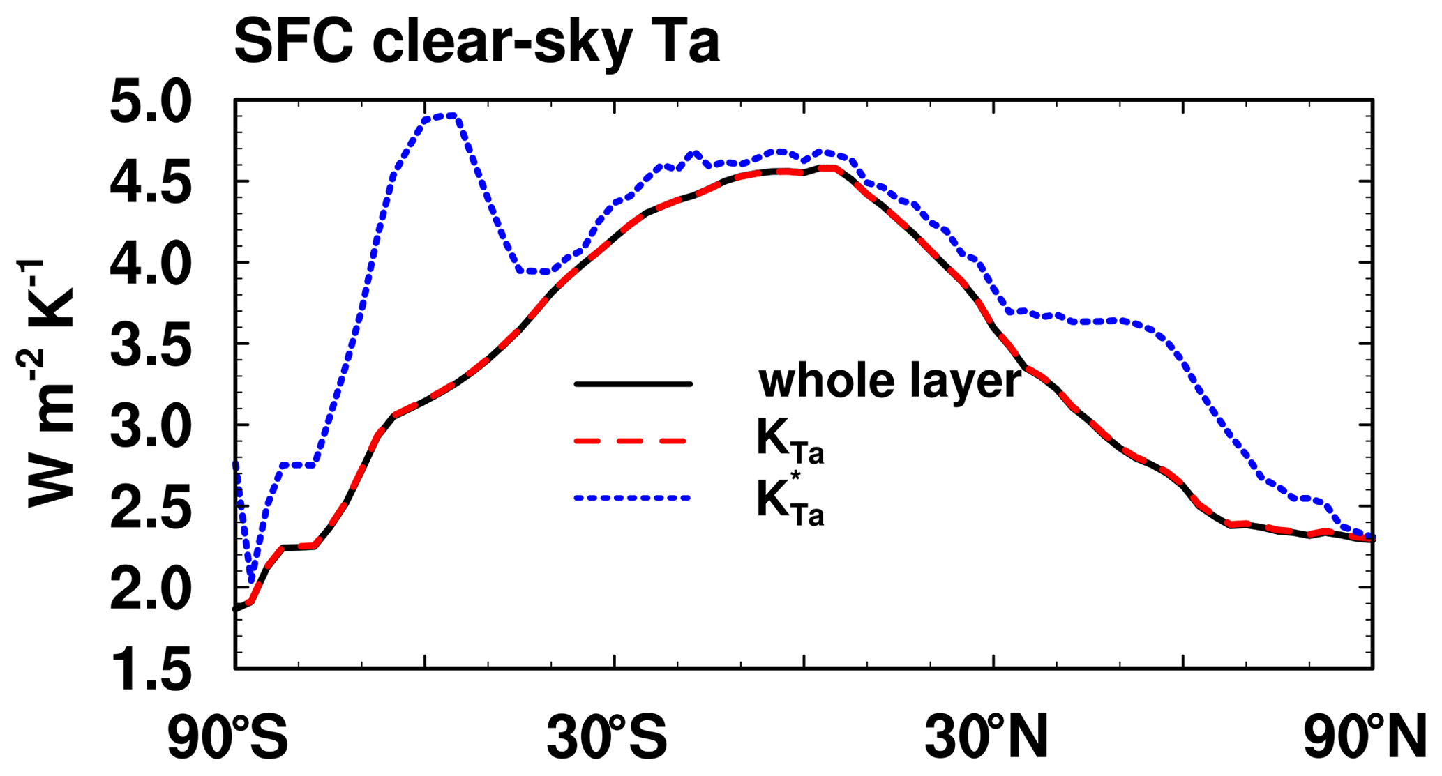
Figure A3 Zonal mean monthly mean air temperature kernels for surface flux from ERA5 in clear sky. Black line is the result from the whole-column perturbation computation by RRTMG, providing a “truth” for comparison. Red dashed line is the kernel weighted with fraction of time ($K_{T_{\mathrm{a}}}$) and blue dotted line represents results without weights ($K_{T_{\mathrm{a}}}^{\ast }$).

Figure A3 illustrates the differences between $K_{T_{\mathrm{a}}}^{\ast }$ and $K_{T_{\mathrm{a}}}$, in terms of their vertically integrated value. Such a difference is pronounced over the Southern Oceans (around 60^∘ S), where the surface pressure value varies considerably. This likely explains why Fig. 3h shows noticeable differences in the air temperature kernel in this region.

A5 Layer-specified and layer-thickness-normalized radiative kernels

We generate two versions of vertically resolved air temperature kernels – the water vapor LW and SW kernels – one with values corresponding to specified vertical layers, i.e., in the units of W m⁻² K⁻¹, and another with unit-layer thickness (e.g., as shown in Figs. 2 and 4), i.e., in W m⁻² K⁻¹ 100 hPa⁻¹. The latter properly portrays the vertical distribution of radiative sensitivity to perturbations in the unit thickness layers, while the former may be more convenient to use in feedback quantifications. For TOA budget analyses, these two versions of kernels lead to little difference in practice due to limited contributions from the bottom atmospheric layer. However, for surface budget analyses, we recommend using the layer-specified kernels, as the surface kernels typically show the strongest sensitivity to the perturbations in the bottom layers, which can be best accounted for in the non-normalized kernels. Otherwise, the difference in surface pressure between ERA5 and GCMs needs to be carefully treated to avoid errors caused, for example, by missing the radiative contribution from the bottom layer of the atmosphere. To illustrate this issue in an example, consider a location (latitude–longitude grid point) where the surface pressure is 960 hPa in a GCM and the lowermost level of the non-zero value of the ERA5 air temperature kernel is located at 975 hPa. Had the air temperature change been set to 0 or an NaN (not a number) value due to the GCM ground level being above 975 hPa, the contribution to the surface radiation change from the air temperature change in the bottom layer of the atmosphere would not be included, which might have led to a biased quantification of the feedback. We recommend interpolating the air temperature changes from the GCM vertical coordinate to the kernel vertical coordinate, using surface values to replace the missing levels (e.g., the 975 hPa level in the above example) before multiplying with the kernel values when computing the feedbacks of air temperature and water vapor.