Reconstructing ocean subsurface salinity at high resolution using a machine learning approach

A gridded ocean subsurface salinity dataset with global coverage is useful for research on climate change and its variability. Here, we explore the feed-forward neural network (FFNN) approach to reconstruct a high-resolution (0.25^∘ × 0.25^∘) ocean subsurface (1–2000 m) salinity dataset for the period 1993–2018 by merging in situ salinity profile observations with high-resolution (0.25^∘ × 0.25^∘) satellite remote-sensing altimetry absolute dynamic topography (ADT), sea surface temperature (SST), sea surface wind (SSW) field data, and a coarse-resolution (1^∘ × 1^∘) gridded salinity product. We show that the FFNN can effectively transfer small-scale spatial variations in ADT, SST, and SSW fields into the 0.25^∘ × 0.25^∘ salinity field. The root-mean-square error (RMSE) can be reduced by ∼11 % on a global-average basis compared with the 1^∘ × 1^∘ salinity gridded field. The reduction in RMSE is much larger in the upper ocean than the deep ocean because of stronger mesoscale variations in the upper layers. In addition, the new 0.25^∘ × 0.25^∘ reconstruction shows more realistic spatial signals in the regions with strong mesoscale variations, e.g., the Gulf Stream, Kuroshio, and Antarctic Circumpolar Current regions, than the 1^∘ × 1^∘ resolution product, indicating the efficiency of the machine learning approach in bringing satellite observations together with in situ observations. The large-scale salinity patterns from 0.25^∘ × 0.25^∘ data are consistent with the 1^∘ × 1^∘ gridded salinity field, suggesting the persistence of the large-scale signals in the high-resolution reconstruction. The successful application of machine learning in this study provides an alternative approach for ocean and climate data reconstruction that can complement the existing data assimilation and objective analysis methods. The reconstructed IAP0.25^∘ dataset is freely available at https://doi.org/10.57760/sciencedb.o00122.00001 (Tian et al., 2022).

1 Introduction

Gridded ocean datasets with complete global ocean coverage are of great importance to marine and climate research (Lyman and Johnson, 2014; Durack et al., 2014; Ciais et al., 2013; Domingues et al., 2008; Bagnell and DeVries, 2021). For example, most climate monitoring applications depend on gridded products (Abram et al., 2019; Ishii et al., 2017; Liang et al., 2021). However, in situ salinity observation data are sparse, owing to the limitations of observation techniques, which brings difficulties to the generation of ocean salinity data products (Roemmich et al., 2019, 2009).

Currently, the estimation of salinity fields mainly relies on two approaches: (1) objective analysis methods based on in situ observations, resulting in so-called objective analysis data products (Gaillard et al., 2016; Hosoda et al., 2008; Roemmich and Gilson, 2009; Cheng and Zhu, 2016; Lu et al., 2020); and (2) data assimilation methods, which combine numerical simulations and observations to result in what is referred to as a reanalysis product (Carton et al., 2018; Forget et al., 2015; Jean-Michel et al., 2021; Balmaseda et al., 2013). The accuracy of the more traditional objective analysis approach is critically dependent on the data coverage and the reliability of spatial covariance, which defines how the information is propagated from data-rich to data-sparse regions (Von Schuckmann et al., 2014; Zhou et al., 2004). Previously available objective analysis products mostly have a horizontal resolution of 1^∘ × 1^∘. The reanalysis approach relies on model simulations which use data assimilation schemes to constrain models with various types of observations, such as in situ and satellite remote-sensing data (Storto et al., 2019; Jean-Michel et al., 2021). Reanalysis products can be strongly impacted by model biases, especially below the ocean surface (Storto et al., 2019; Balmaseda et al., 2015). However, Palmer et al. (2017) and Cheng et al. (2020) indicated that such reanalysis products have much larger spread than observational products for ocean heat content (temperature) and ocean salinity, suggesting caution when adopting the data assimilation approach in some applications such as long-term climate change.

As higher-resolution observational data are crucial for evaluating models/reanalysis and understanding ocean processes at multiple scales, such as the mesoscale and sub-mesoscale (McWilliams, 2016), high-quality observational datasets with resolutions higher than 1^∘ × 1^∘ could be useful for ocean and climate research, e.g., resolving the vertical structure of warm and cold eddies. To reconstruct an observational dataset with resolution higher than 1^∘ × 1^∘, remote-sensing observations are essential, as they can be used to incorporate smaller-scale signals that are insufficiently sampled by in situ salinity profile observations. Two types of approaches have been used previously to propagate surface information to the subsurface: dynamical and statistical. The dynamical approach adopts physical relationships between surface and subsurface variables. For example, Wang et al. (2013) proposed an isQG (interior + surface quasi-geostrophy) method, using information such as sea surface height (SSH), sea surface temperature (SST), and sea surface salinity (SSS) to invert the density and velocity fields of the ocean interior. The statistical approach utilizes historical data to establish a statistical relationship between remote-sensing observations and subsurface observations (e.g., linear regression between surface height and subsurface temperature/salinity). Some of the available statistical relationships have been derived by multiple linear regression models (Warin, 2019), empirical orthogonal functions (Hannachi et al., 2007), and the gravest empirical mode method (Liu et al., 2021). However, both dynamical and statistical approaches have obvious limitations. The dynamical approach is overly dependent on physical assumptions, which are always simplified, such as relying on surface quasi-geostrophic dynamics to derive subsurface signals from surface changes. Caveats of the statistical approach is the lack of physical constraints and the simplified assumptions. For example, some approaches have simplified the nonlinear relationship between surface dynamic height and subsurface temperature/salinity to a linear relationship.

Compared with traditional reconstruction methods, machine learning approaches do not rely on any simplified assumptions in the process of data reconstruction and are able to learn and fit parameters automatically. There have been some attempts recently; for example, Wang et al. (2021) used remote-sensing data and neural network methods to estimate the subsurface temperature in the western Pacific. Combining satellite data and Argo gridded products, Su et al. (2020) used neural networks to estimate ocean heat content anomalies over four different depths down to 2000 m. Lu et al. (2019) estimated the subsurface temperature through a clustering neural network method based on SST, SSH, and wind field measurement data. Although these studies provide some hints that machine learning approaches can be useful in data reconstruction applications, there are still some limitations. First, some studies (Lu et al., 2019; Su et al., 2020; Wang et al., 2021) used Argo gridded data as the “truth” to train the machine learning model; thus the reconstruction error in the Argo gridded data is embedded in the final reconstruction. Second, the spatial resolution of the most reconstructed data is still 1^∘ × 1^∘. The added value of high-resolution remote-sensing data is not maximized; for example, the resultant 1^∘ × 1^∘ field is still insufficient to resolve mesoscale signals. Finally, previous reconstructions have tended to focus mainly on temperature rather than salinity, and a comprehensive assessment of the uncertainty has always been absent. In addition, due to the lack of interpretability of the machine learning approach, a thorough comparative evaluation with traditional methods is clearly a crucial line of study.

This paper explores the feed-forward neural network (FFNN) approach to reconstruct a high-resolution (0.25^∘ × 0.25^∘) ocean subsurface (1–2000 m) salinity dataset for the period 1993–2018 by merging in situ profile observations (processed to a gridded 0.25^∘ × 0.25^∘ arithmetic mean field in this study, detailed in the following text) with high-resolution satellite remote-sensing altimetry absolute dynamic topography (ADT), SST, sea surface wind (SSW) data, which included zonal (USSW) and meridional (VSSW) components, and a coarse-resolution IAP1^∘ gridded salinity product from the Institute of Atmospheric Physics (IAP). The first objective is to understand how well the FFNN approach works for data reconstruction using the ocean salinity field as an example. Second, the new machine-learning-based high-resolution (0.25^∘ × 0.25^∘) salinity dataset will be comprehensively evaluated in this study, which facilitate its further applications. The added value of remote-sensing data in a high-resolution salinity reconstruction is demonstrated and discussed.

The rest of the paper is organized as follows: the data and methods employed in our study are presented in Sect. 2. The performance of the dataset in terms of geographical pattern, regional analysis, and overall reconstruction performance is assessed in Sect. 3. The uncertainty of the FFNN approach is examined in Sect. 4. An analysis of the major climatic patterns is conducted in Sect. 5. Importance of each feature for the reconstruction is described in Sect. 6. Data availability is described in Sect. 7. The results of the study are summarized and discussed in Sect. 8.

2 Data and methods

2.1 Input data

2.1.1 Remote-sensing and IAP1^∘ observational data

The ADT data extracted from the European Copernicus Marine Environment Monitoring Service (CMEMS) were computed based on altimeter data from several satellites including Jason-3, Sentinel-3A, HY-2A, Saral/AltiKa, Cryosat-2, Jason-2, Jason-1, T/P, ENVISAT, GFO, and ERS1/2 (Mertz et al., 2016). The dataset has a spatial resolution of 0.25^∘ × 0.25^∘ and a daily temporal resolution covering the period from January 1993 to December 2020.

The SST data were extracted from the daily Optimum Interpolation Sea Surface Temperature (OISST) v2.1 data, provided by the National Oceanic and Atmospheric Administration (NOAA). OISST is produced by interpolating SST observations from different sources, resulting in a smoothed field with complete global ocean coverage. The sources of data are satellite (Advanced Very High Resolution Radiometer) and in situ platforms (i.e., ships and buoys) (Banzon et al., 2016; Reynolds et al., 2007; Huang et al., 2021). Data are currently available from 1 September 1981 to the present day, with a spatial resolution of 0.25^∘ × 0.25^∘ and a daily temporal resolution.

The SSW data were extracted from the Cross-Calibrated Multi-Platform (CCMP) V2 monthly dataset (Wentz et al., 2016), provided by the National Center for Atmospheric Research (NCAR). The processing of CCMP V2 now combines Version-7 Remote Sensing Systems radiometer wind speeds, QuikSCAT and ASCAT scatterometer wind vectors, moored buoy wind data, and ERA-Interim model wind fields using a variational analysis method to produce 0.25^∘ × 0.25^∘ gridded vector winds (Atlas et al., 2011). The dataset covers the period from July 1987 to April 2019.

The IAP1^∘ salinity data give a global coverage of the oceans at a horizontal resolution of 1^∘ × 1^∘ in 41 vertical levels from 1 to 2000 m and a monthly temporal resolution from 1940 to the present day (Cheng and Zhu, 2016; Cheng et al., 2017). This product combines in situ salinity profiles with coupled model simulations (from phase 5 of the Coupled Model Intercomparison Project) to derive an objective analysis with the ensemble optimal interpolation approach (Cheng et al., 2020). The product is designed to minimize the sampling error in representing large-scale and long-term climate changes and variabilities.

All of the above-mentioned products were processed into monthly averages, and IAP1^∘ data were linearly interpolated to unified 0.25^∘ × 0.25^∘ resolution fields, which were used as inputs for the FFNN approach.

2.1.2 In situ salinity observations

In situ ocean salinity observations were sourced from the World Ocean Database (WOD) (Boyer et al., 2018). Data from all available instruments (e.g., Argo; Nansen bottle; conductivity–temperature–depth, CTD) were used in this study. Quality flags from WOD were applied (only “good data” with a flag equal to zero were used). All of the profiles were first interpolated to a standard 41 vertical levels between 1 and 2000 m, as in the IAP1^∘ data. Then, 12-monthly climatologies were constructed using all data from 1990 to 2010 (centered around 2000), and anomaly profiles are derived by subtracting monthly climatologies from salinity profiles. Finally, the salinity anomalies were averaged into 0.25^∘ × 0.25^∘, 1-month, and 41-level grid boxes via simple arithmetic averaging, without spatial interpolation and smoothing. The reconstructions are applied to the anomaly fields, similar to previous objective analyses because of the larger spatial decorrelation length scale of the anomaly fields than the absolute fields (i.e., Levitus et al., 2009; Cheng et al., 2017). The gridded averaged salinity anomalies were regarded as the “truth” to train the FFNN approach during the reconstruction. The gridded averages were used instead of the raw profiles because they were able to minimize the impact of spatial heterogeneity of the raw profiles, reduce the subgrid (<0.25^∘) variability and observational noise, and improve the computational efficiency (Cheng et al., 2017, 2020; Gaillard et al., 2016; Good et al., 2013; Ishii et al., 2003, 2017; Levitus et al., 2012; Lyman and Johnson, 2014; Roemmich et al., 2009).

2.2 Independent ocean products for evaluation and comparison

Three independent ocean products were used to assess the quality of the newly reconstructed high-resolution salinity data in this study (hereafter denoted as IAP0.25^∘), ARMOR3D data, SMAP satellite data, and EN4 gridded data.

The ARMOR3D V4 dataset was extracted from CMEMS, which is a global three-dimensional temperature and salinity dataset with high horizonal (0.25^∘ × 0.25^∘) spatial resolution from 0–5500 m (Guinehut et al., 2012; Mulet et al., 2012). The spatial coverage ranges from 82.125^∘ S to 89.875^∘ N and 0.125 to 359.875^∘ E. The ARMOR3D combines satellite observation data (ADT, geostrophic surface currents, SST) and in situ temperature and salinity profile data through a multivariate/simple linear regression and an optimal interpolation method. This product offers four versions with different temporal resolutions: near-real-time weekly data, near-real-time monthly data, multi-year reprocessed weekly data, and multi-year reprocessed monthly data. The multi-year reprocessed monthly data were used in this study.

The SMAP V4 dataset is provided by NOAA and comprises monthly 0.25^∘ × 0.25^∘ resolution SSS data. The SMAP data are based on satellite observations and have the capability to monitor the global SSS field in near real time, with mesoscale information resolved for salinity (Vinogradova et al., 2019).

The EN4 gridded data were obtained from the UK Met Office. The EN4 dataset uses an optimal interpolation method to construct the ocean subsurface gridded salinity field based on in situ salinity profile data. We chose the EN4-GR10 version (Gouretski and Reseghetti, 2010), which has a spatial resolution of 1^∘ × 1^∘ and 42 vertical levels from 5 to 5500 m and temporal coverage from 1940 to 2018 (Li et al., 2019).

Table 1 A list of the input datasets and validation products used in this study.

2.3 Methods

2.3.1 Feed-forward neural network

The FFNN was used to reconstruct the subsurface salinity anomalies in this study. We chose FFNN because it has been shown to be superior to the other three widely used machine learning approaches in reconstructing ocean parameters (Lu et al., 2019; Stamell et al., 2020; Wang et al., 2021). Our own evaluation based on synthetic data and salinity observations (see Supplement) also reveals that FFNN is a robust approach and leads to the smallest error compared with other approaches (e.g., light gradient boosting machine, LightGBM) (Gan et al., 2021). An FFNN is a one-way, multi-layer structure network that includes an input layer, hidden layers, and an output layer (Abdar et al., 2021; Contractor and Roughan, 2021; Gabella, 2021). The zero layer is called the input layer, the last layer is called the output layer, and the other intermediate layers are called the hidden layers. The neurons in the FFNN are arranged in layers, with each neuron belonging to a different layer. The neurons of each layer are fully connected; that is, each neuron is connected to the neurons of the previous layer and the next layer. The information in the network will only flow from the input layer to the hidden layers and then to the output layer; that is, the output of the previous layer is used as the input of the next layer, and the information of the next layer has no effect on the previous layer. Each layer of the FFNN is equivalent to a function, and the connection of the multi-layer network is equivalent to a composite function to form a linear or nonlinear mapping from input variables to output variables. The complexity of the FFNN depends not only on how many neurons or layers are chosen, but also on the type of layers and activation functions.

All the input parameters of the model training were converted to anomalies by subtracting their respective climatologies for 1993–2015. For example, the input data were the IAP1^∘ salinity anomalies (IAP1SA), the absolute dynamic topography anomalies (ADTA), sea surface temperature anomalies (SSTA), and sea surface wind anomalies (SSWA), which included zonal and meridional anomalies (USSWA/VSSWA). The standardization of data can improve the convergence speed of the neural network method (LeCun et al., 2012). The method proposed by Denvil-Sommer et al. (2019) was used to perform sine/cosine transformations of latitude, longitude, and time. The Z score standardization method was used to process the ADTA, SSTA, USSWA, VSSWA, IAP1SA, and standard layer depth parameters.

The structure of the FFNN used in this study is illustrated in Fig. 1, in which y is the gridded salinity anomaly, regarded as a “true value”. The input x includes longitude, latitude, time, depth, IAP1SA, ADTA, SSTA, USSWA, and VSSWA.

A training/testing approach was adopted to determine the key parameters and settings for the FFNN. The full salinity dataset was randomly divided into a training set (80 % of the whole dataset) and a test set (20 % of the whole dataset). The training set was used to fit the FFNN algorithm, and the test set was used for performance evaluation. The root-mean-square error (RMSE) was calculated between the reconstruction and the test dataset as a model evaluation metric. Once the RMSE begins to increase, the training iteration stops, and the best parameters and settings are stored. A grid search strategy (Liashchynskyi et al., 2019) was used to optimize the structure of the neural network. The optimized neural network we used consists of one input layer, one output layer, and four hidden layers; the number of neurons in each hidden layer was set to 256, 128, 64, and 32; the activation function was the rectified linear unit; the optimizer was the root-mean-square propagation (RMSProp) (Bushaev, 2018); the learning rate was 0.001; and the cost function was minimized for training as follows:

$$\begin{array}{}\text{(1)}& J\left({\mathit{\theta }}_{\mathrm{0}},{\mathit{\theta }}_{\mathrm{1}},\mathrm{\dots }{\mathit{\theta }}_n\right)={\displaystyle \frac{\mathrm{1}}{\mathrm{2}m}}\sum _{i=\mathrm{1}}^m{\left(h_{\mathit{\theta }}\left(X^{\left(i\right)}\right)-y^{\left(i\right)}\right)}^{\mathrm{2}},\end{array}$$

where X= (longitude, latitude, depth, time, IAP1SA, ADTA, SSTA, USSWA, VSSWA), y denotes the “truth values”, m is the number of samples, h_θ is the FFNN model for training, θ is the parameter of the model, and the training objective is the minimum J.

Bayesian regularization (Dan Foresee and Hagan, 1997) and dropout were used during model training to maintain generalization and prevent overfitting. Since the Bayesian regularization algorithm does not require cross-validation to ensure generalization, no validation set was defined in this process (Lu et al., 2019; Wang et al., 2021). Adopting these settings and parameters, the final FFNN model used for reconstruction was trained by the full salinity dataset to ensure the best performance.

Figure 1 Schematic diagram of subsurface salinity reconstruction by the FFNN approach.

2.3.2 The 5-fold cross validation

To evaluate the reconstruction using independent test data, a 5-fold cross validation approach was used (Gui et al., 2020). This type of validation is one of the most popular models in statistics and machine learning (Berrar, 2018; Lei, 2020). In the 5-fold cross validation, the full observational datasets were split into training (80 %) and testing (20 %) datasets. The training set was used to train the machine learning model and then to derive the reconstruction. The testing dataset was used as an independent dataset to verify the performance of the reconstruction. To effectively construct the training and testing datasets, the full observational data 0.25^∘ × 0.25^∘ gridded average fields, as introduced before, were randomly split into five subsets. In each run, four subsets were used for training, and the remaining subset was used for testing. This process was repeated four times so that each of the five subsets could be used as the testing dataset. In this way, the 5-fold cross validation needed to be trained five times to ensure that all the data participated in both the training and testing. By calculating the difference between the reconstructed data and the truth value of the independent testing data, the machine learning method could be evaluated.

2.3.3 Uncertainty quantification

The uncertainty of the final reconstruction will stem from three sources: instrumental error, representativeness error, and reconstruction error. The instrumental error is related to the instrument accuracy of a salinity measurement. For instance, the accuracy of most Argo salinity data is about ±0.01 psu. However, many Argo floats suffer from sensor drift, so the error is much larger for some data, which has yet to be quantified (Wong et al., 2020). For the validated marine mammal data, the accuracy can be ±0.03 psu (Siegelman et al., 2019). The CTD data accuracy is about ±0.01 psu. The representativeness error defines the accuracy of the gridded average in representing the true average of salinity in this grid. This error is associated with the sampling of ocean changes inside each 0.25^∘ and 1-month grid: insufficient sampling will lead to errors in the grid average. The magnitude of error depends on the spatiotemporal variability in each grid box: larger subgrid variability requires more data to accurately estimate the grid average. The reconstruction error defines the accuracy of the gap-filling, i.e., the machine learning approach in this study. This error is related to the errors in the FFNN model's design and parameter choice, etc. To quantify the uncertainty in the reconstruction, these three major error sources had to be properly accounted for.

This study adopted a probabilistic approach to the propagation of errors and to quantify the uncertainty. We perturbed the interpolated 0.25^∘ gridded average fields five times with prescribed instrumental and representativeness uncertainty and then obtained five perturbed gridded fields. The FFNN was then applied to these five perturbed fields, separately, to result in five reconstructions at each time with a Monte Carlo dropout approach (Gal and Ghahramani, 2016; Abdar et al., 2021). This process led to 25 ensemble members in the final reconstruction, the spread of which was used to quantify the uncertainty.

The perturbations were performed as follows. For instrumental error, we perturbed each individual salinity profile by its instrumental accuracy, assuming a Gaussian distribution with zero mean and the instrumental accuracy as the standard deviation. The perturbed profiles were then used to construct the gridded average fields (0.25^∘ and 1-month grid). On this basis, the representativeness error was included by perturbing each gridded average by a Gaussian distribution with zero mean and standard deviation of Var$/\sqrt{n}$, where “Var” is a measure of subgrid variability (<0.25^∘ and <1-month), and n is the number of profiles to calculate the grid mean. The Var is static (non-time-varying) and calculated by the standard deviation of the salinity data in each 1^∘ grid box when there were >10 measurements. Grid boxes of 1^∘ were used here because of the data scarcity, which would overestimate the subgrid variability of <0.25^∘. However, this overestimation could compensate for the unresolved/unknown errors, such as salinity drift. The results are presented in Fig. 2a and c. The figures reveal incomplete ocean coverage. Thus, we interpolated this field using an objective interpolation method (Fig. 2b and d) (Cheng et al., 2017). A spatial decorrelation length scale of 8^∘ was used, which is consistent with a previous gap-filling approach for ocean temperature and salinity (Levitus et al., 2012). A global estimate of salinity Var in Fig. 2b and d shows that the coastal regions, boundary current systems, and Antarctic Circumpolar Current (ACC) regions have larger Var than other places because of either river runoff or mesoscale and sub-mesoscale variabilities. The estimated Var and the number of data n in each 0.25^∘ and 1-month grid box were combined to perturb the local 0.25^∘ and 1-month grid mean, assuming a Gaussian distribution, which resulted in five perturbed 0.25^∘ and 1-month gridded average fields and inputs into the FFNN approach.

The Monte Carlo dropout approach was employed to estimate the uncertainty due to the FFNN approach. This is one of the most popular ways to estimate machine learning method uncertainty, and it does not require any change to the existing model architecture (Stoean et al., 2020; Milanés-Hermosilla et al., 2021). Monte Carlo dropout was operated by randomly dropping some units of the neural network during the model training process. In this way, the approach and parameter uncertainty could be accounted for. In this study, we applied the FFNN to the five above-derived perturbed fields separately to create five reconstructions each time with the Monte Carlo dropout approach. Then, the spread (i.e., standard deviation) of the $\mathrm{5}\times \mathrm{5}=\mathrm{25}$ final reconstructions was used to quantify the total uncertainty. With this approach, all major error sources were propagated to the final fields, where the Monte Carlo dropout approach considers the reconstruction uncertainty of the FFNN, and the five perturbed gridded fields represent the instrumental and representativeness uncertainty.

Figure 2 The estimated Var (a quantification of salinity subgrid variability) of in situ observations in this study. The original (a, c) and objectively analyzed fields (b, d) are presented for the depths of 20 m (a, b) and 300 m (c, d), respectively, as two examples.

2.3.4 Evaluating the relative importance of different inputs

In this paper, we used an approach named Kernel SHAPley Additive exPlanations (SHAP) to evaluate the contribution of different input parameters (Lundberg and Lee, 2017).

SHAP is a method inspired by game theory to explain the contribution of each feature to the model output. It works for any model and is especially useful for interpreting black box models (e.g., FFNN). It approximates the original model with a sum of linear terms. Like linear regression models, each term is the contribution of the corresponding feature to the model output. To compute the linear terms, combinations of features are examined. A total of p features is assumed. For a given combination of k features out of the original p, feature j is dropped and added back to the combination. The change of model performance is a marginal contribution of the feature j. Repeat the same process for all combinations of features from k=1 to p. The aggregated marginal contribution over all combinations is the contribution of the feature j to the model output.

With this approach, SHAP can quantify the average impact of an input on the final output (reconstruction in our case). The change in the output is representative of the importance of the input for predicting the output, which is called the SHAP value. By comparing the SHAP value for each input, the relative contribution to the final reconstruction can be assessed.

To implement SHAP, the Kernel SHAP algorithm was employed, which makes no additional assumption about the model type (e.g., linear models, tree models, and deep network models). The disadvantage of the SHAP algorithm is that it is slower than other model-type-specific algorithms. The SHAP algorithm is too computationally expensive to apply for the full dataset (Chau et al., 2021). Pauthenet et al. (2022) indicated that ∼0.44 % of the total samples is sufficient to obtain stable results for ocean temperature and salinity reconstruction in the Gulf Stream region. Therefore, we follow their choice and randomly selected 0.5 % of data to calculate the Shapley value for each input parameter (expanding it to 1 % did not make significant difference based on our test). The importance of each input is estimated by the average of absolute Shapley values for each input, which is then normalized by the sum of the absolute Shapley values to derive the relative importance of each input.

3 Reconstruction results

This section presents the reconstruction results and discusses their reliability using multiple examples and thorough statistical analyses.

3.1 Reconstruction of the geographical pattern

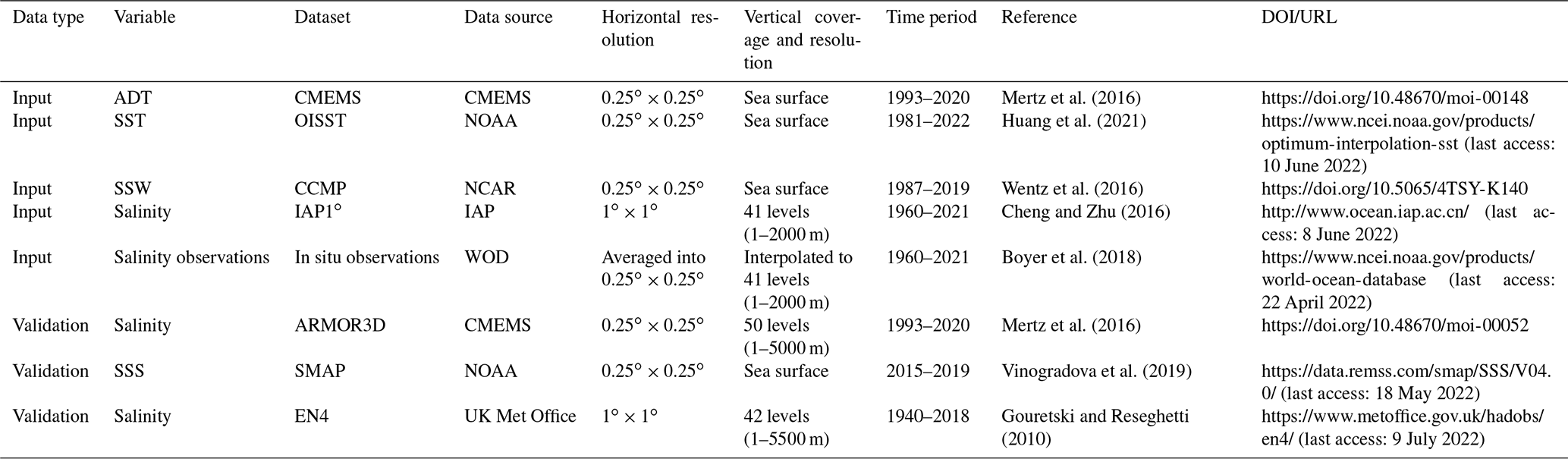
We first examine the geographical distribution of the reconstructions for January 2016 as an example. January 2016 was chosen arbitrarily for illustration purposes. Using other times yielded similar results. Figures 3 and 4 show the salinity anomalies of the new reconstruction, IAP0.25^∘, in comparison with the IAP1^∘, ARMOR3D, ADTA, SSTA, and in situ observations of January 2016 at 100 and 300 m, respectively. It appears that the large-scale pattern of the IAP0.25^∘ salinity field is closely consistent with the distribution of IAP1^∘ and ARMOR3D, as revealed by in situ data. There are significant negative salinity anomalies in the tropical Pacific, intertropical convergence zone (ITCZ), and the Pacific north of the Equator, as well as positive salinity anomalies in the Southeast Pacific, Northwest Pacific, and the east coast of Australia. Compared with the very smooth field of IAP1^∘, the IAP0.25^∘ salinity field includes more small-scale signals. Such information must come from in situ data and ADT/SST and USSW/VSSW fields, as they have finer resolution. The previous IAP1^∘ salinity data mainly reveal large-scale patterns, and there are almost no eddies in the Gulf Stream and the Kuroshio extension regions. The comparison between IAP0.25^∘ and IAP1^∘ reveals a bigger difference in boundary currents and ACC regions with rich eddies.

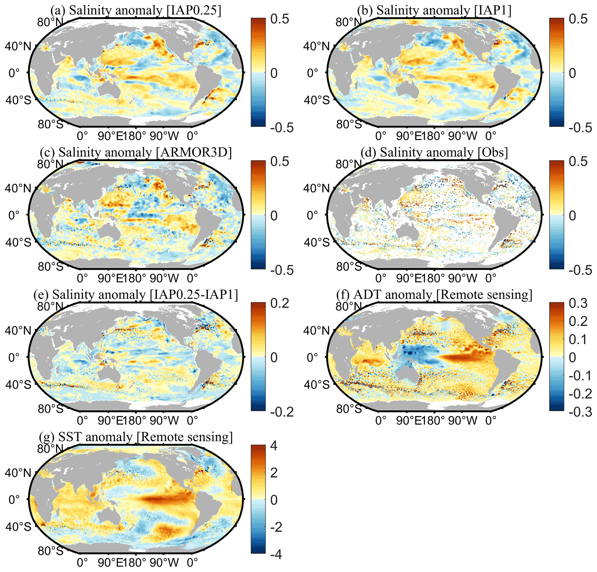
Figure 3 Spatial distribution of salinity anomalies of (a) IAP0.25^∘, (b) IAP1^∘, (c) ARMOR3D, (d) in situ observations, and (e) IAP0.25^∘ minus IAP1^∘ at 100 m, as well as the spatial distribution of (f) ADTA and (g) SSTA in January 2016.

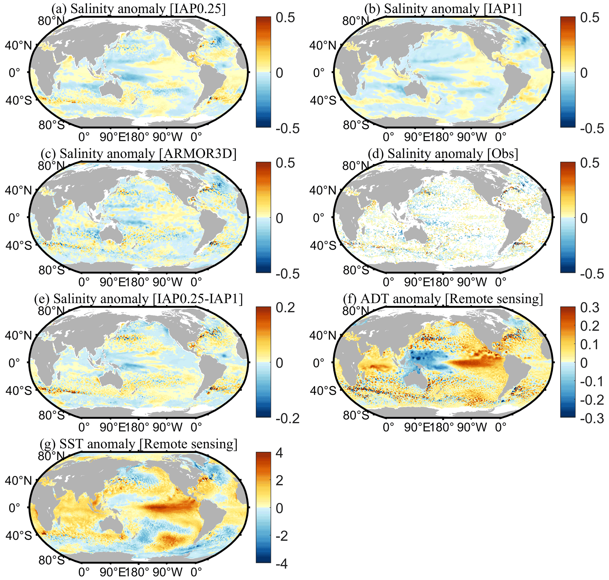
Figure 4 Spatial distribution of salinity anomalies of (a) IAP0.25^∘, (b) IAP1^∘, (c) ARMOR3D, (d) in situ observations, and (e) IAP0.25^∘ minus IAP1^∘ at 300 m, as well as the spatial distribution of (f) ADTA and (g) SSTA in January 2016.

To get a closer look at these critical regions, we concentrate on the salinity reconstruction in the boundary currents regions, e.g., the Gulf Stream (Fig. 5) and the Kuroshio Extension (Fig. 6). Both of these areas are active with mesoscale eddies (Chassignet et al., 2020; Cheng et al., 2014; Frenger et al., 2015; Rhines, 2019), and with very strong net energy growth and net dissipation of mesoscale eddies (Xu et al., 2013).

In the Gulf Stream region (Fig. 5), at a depth of 100 m, IAP1^∘, IAP0.25^∘, and ARMOR3D all reveal large-scale positive salinity anomalies along the North Atlantic coastal regions, negative anomalies in the middle and east, and positive anomalies extending from southwest (80^∘ W, 15^∘ N) to the northeast (20^∘ W, 30^∘ N). The 300 m salinity shows similar patterns as that at 100 m, except for larger areas of positive anomalies from southwest to northeast. The similarity among the large-scale patterns yielded by the datasets suggests the large-scale reconstruction is reliable. However, there are obvious differences between the four datasets in their ability to describe the fine-scale structures. For example, at 100 m, the reconstructed (IAP0.25^∘) field and ARMOR3D show more detail in the salinity structure, especially near the boundary currents and coastal regions, compared to IAP1^∘. These anomalies are more consistent with the in situ salinity observations (Fig. 5a–c vs. 5d; Fig. 5e–g vs. 5h).

In the Northwest Pacific Ocean (Fig. 6), IAP1^∘, IAP0.25^∘, and ARMOR3D indicate a large area of positive salinity anomalies in the Northwest Pacific south of 40^∘ N at a depth of 100 m and negative anomalies north of 40^∘ N. A very smooth transition zone along ∼40^∘ N is apparent for IAP1^∘ (Fig. 6b), but IAP0.25^∘ and ARMOR3D suggest a zone with rich mesoscale variabilities (Fig. 6a and c). These findings are more physically plausible because it is the Kuroshio extension region (Chassignet et al., 2020). Even down to 300 m, there are still rich mesoscale structures seen in the observations within 30–40^∘ N (Fig. 6h), as represented by both IAP0.25^∘ and ARMOR3D.

A closer look into the two regions suggests that the new IAP0.25^∘ data can resolve the mesoscale signals in the boundary flow area. However, it also appears that the small-scale anomalies are stronger in the ARMOR3D data than the IAP0.25^∘ data, which is likely associated with the methodological differences. A comparison between in situ observations and IAP0.25^∘ (Figs. 5a vs. 5d; 5e vs. 5h; 6a vs. 6d; 6e vs. 6h) suggests a closer correspondence of IAP0.25^∘ data with observations than ARMOR3D, and a more thorough statistical analysis of the errors will be presented in subsequent sections.

Figure 5 The geographical distribution of salinity anomalies in the Gulf Stream region for IAP0.25^∘, IAP1^∘, ARMOR3D, and in situ observations in January 2016: (a–d) 100 m and (e–f) 300 m.

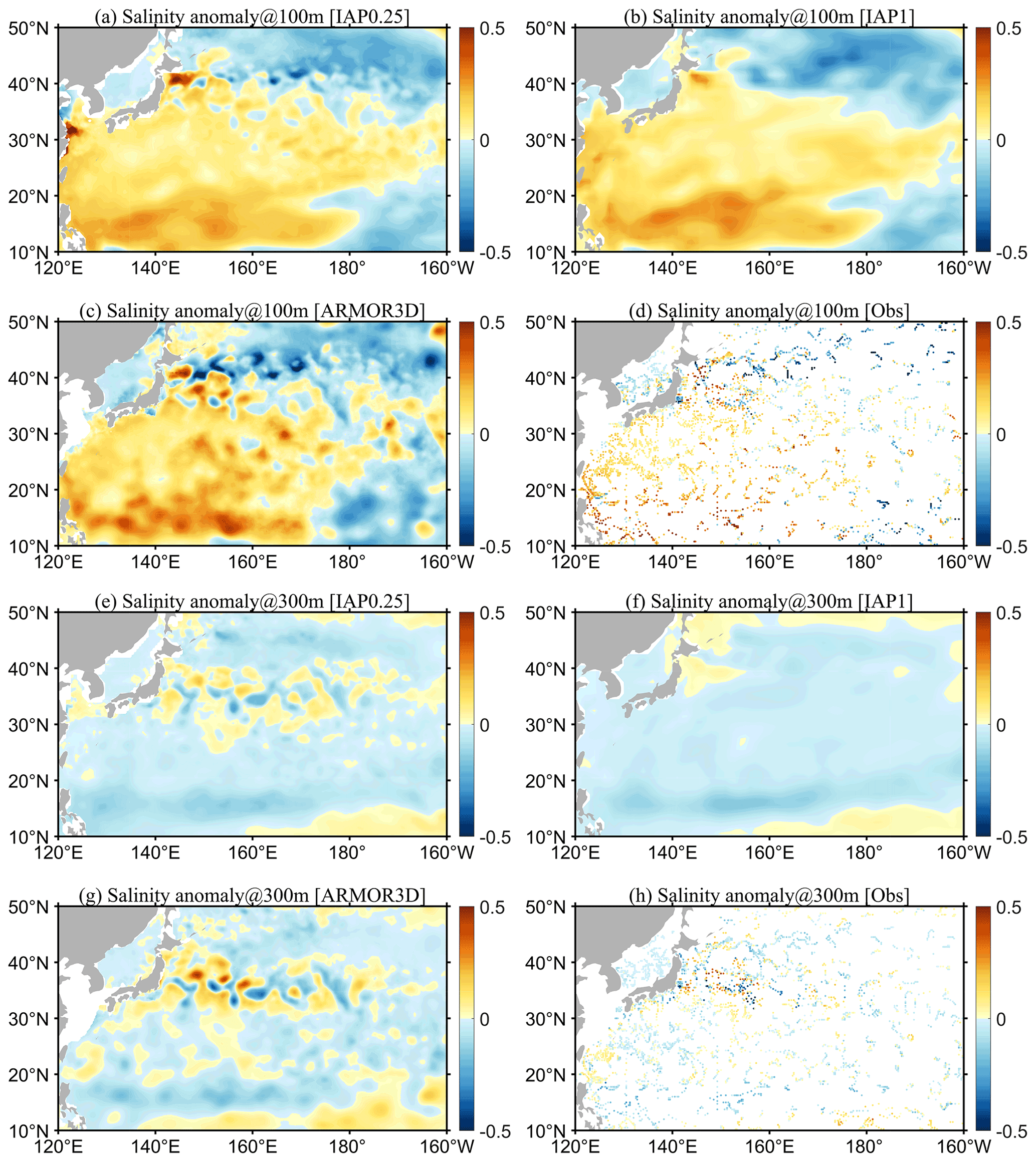
Figure 6 The geographical distribution of salinity anomalies in the Kuroshio and its extension region for IAP0.25^∘, IAP1^∘, ARMOR3D, and in situ observations in January 2016: (a–d) 100 m and (e–f) 300 m.

3.2 Reconstruction of the vertical structure

In addition to the spatial distribution at a given layer, it is desirable to investigate the vertical structure of the salinity field (i.e., to what extent the vertical structure can be restored by the new approach). This section seeks to address this question with two examples: in the Gulf Stream region (along 35.375^∘ N) and in the Kuroshio extension region (along 35.375^∘ N) (Figs. 7 and 8).

Along the Gulf Stream section, satellite remote-sensing SSS data (Fig. 7a), independent from our analysis, suggest a general negative salinity anomaly associated with substantial variability. This reveals the existence of both large-scale change and mesoscale variability. It can be seen from Fig. 7b and d that both the IAP0.25^∘ and IAP1^∘ anomalies are generally negative near the sea surface, indicating the near-surface signals can be restored with IAP0.25^∘. The smoothness of the IAP1^∘ data is associated with its mapping method (Cheng and Zhu, 2016), which focuses more on the large-scale patterns and effectively filters out small-scale variations. Moreover, the small-scale, along-section fluctuations revealed by the in situ profile data (Fig. 7c) are well reflected in the IAP0.25^∘ (Fig. 7d) but not in the IAP1^∘ data (Fig. 7b), highlighting that IAP0.25^∘ is capable of correctly reflecting the small-scale features. ADT data reflect the integrated effect or thermosteric (linked to temperature) and halosteric (linked to salinity) effects over the full volume (Llovel and Lee, 2015; Wang et al., 2017). To the first order, in the thermocline regions, the ADT change should correspond better with thermocline change (first baroclinic mode); thus the salinity change near the thermocline should resemble the ADT in many places. This is supported by Fig. 7 (Fig. 7a vs. 7d), for example, the large positive anomaly near 48, 60, and 68^∘ W revealed by both the in situ salinity profile and ADT data. This indicates a positive contribution of ADT to the reconstruction.

Along the Kuroshio extension section (Fig. 8), the SST and ADT are more consistent with each other than in the Gulf Stream (Fig. 7). There is a deep mixed layer (deeper than 500 m) in this region, so ADT is more influenced by mixed-layer dynamics. In this case, both ADT and SST could support the high-resolution salinity reconstruction because mixed-layer dynamics are associated with strong air–sea heat and freshwater exchanges. For example, the high ADT, SST, and salinity anomalies at 155–160^∘ E and around 180^∘ E and negative anomalies at 178^∘ E and other places in the upper 500 m are all consistent (Fig. 8a, c, d).

In summary, the investigation of these two specific cases increases the degree of confidence in the reconstruction. It seems that mesoscale structures can be realistically restored.

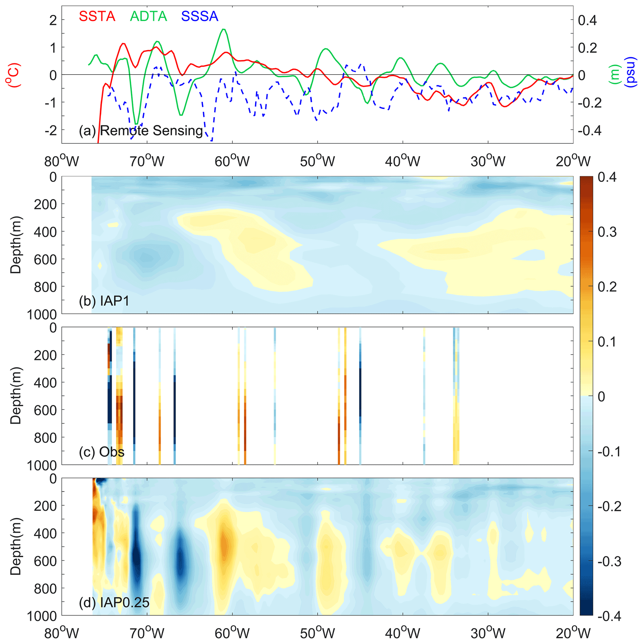
Figure 7 The distribution of SSTA (left y axis), ADTA, and SSS anomalies (SSSA) observed by SMAP on the sea surface (ADTA and SSSA share the right y axis), as well as the vertical section along 35.375^∘ N of the observational in situ salinity anomalies, subsurface salinity anomalies from IAP1^∘, and IAP0.25^∘ gridded data in the Gulf Stream region.

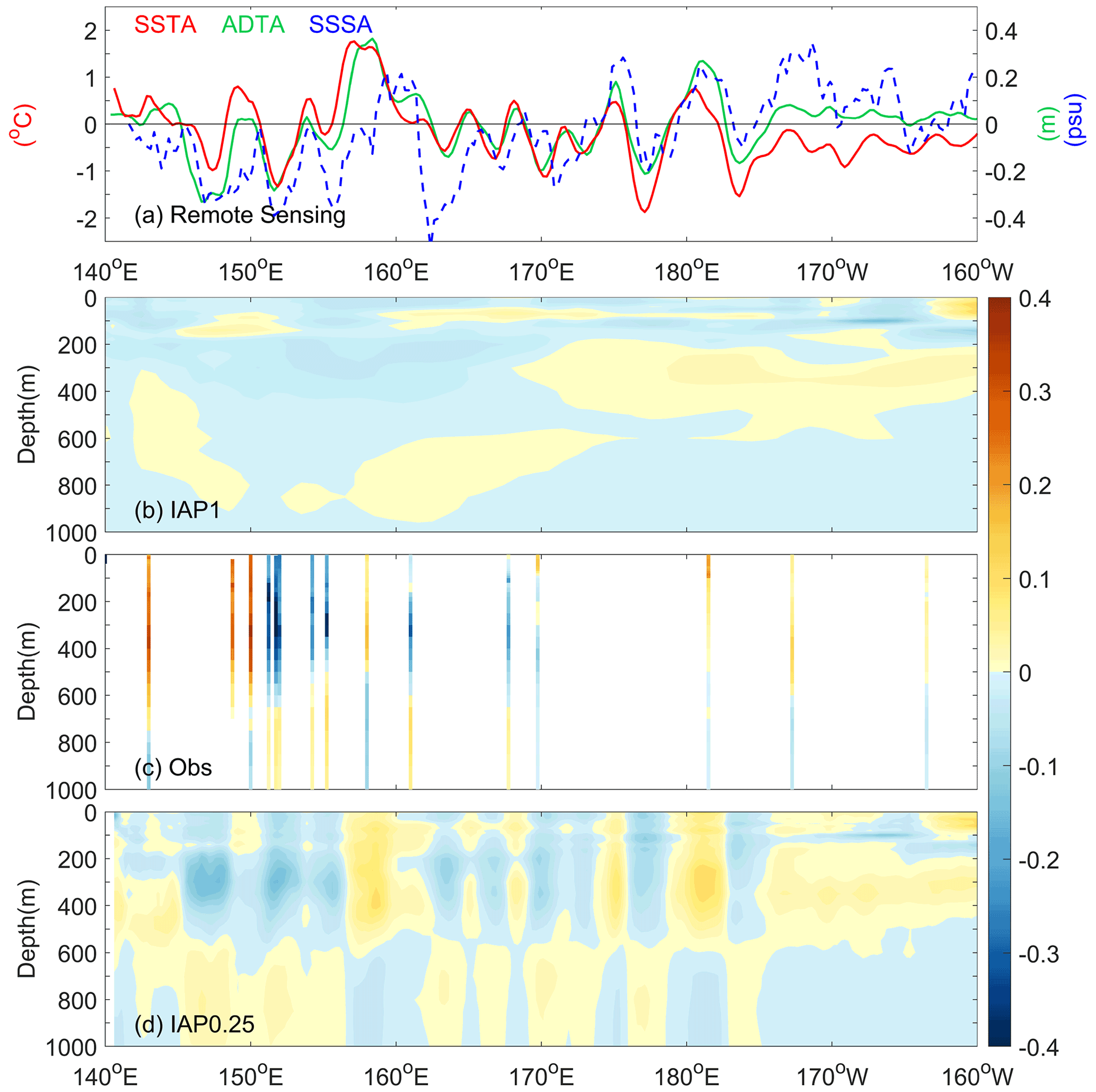
Figure 8 As in Fig. 7 but for the Kuroshio and its extension region along 35.375^∘ N in January 2016.

3.3 Overall reconstruction performance

In the previous two sections, examples were presented to illustrate the reconstruction performance. However, a more thorough statistical examination is still required, which is provided in this section. To quantify the overall error compared with observations, we calculated the RMSE between IAP0.25^∘, IAP1^∘, ARMOR3D, EN4, and the observation data, respectively (denoted as IAP0.25_RMSE, IAP1_RMSE, ARM_RMSE, and EN4_RMSE), and the results are presented in Fig. 9a–d at different layers from the surface down to 2000 m over the globe and in three major basin regions during 1993–2018. Figure 9e–h show the differences between IAP1_RMSE, ARM_RMSE, EN4_RMSE, and IAP0.25_RMSE. First, IAP0.25_RMSE is smaller than all other data products for both global and basinal average. At a global scale, the maximum values are 0.37 psu for IAP0.25_RMSE, 0.50 psu for IAP1_RMSE, 0.55 psu for ARM_RMSE, and 0.56 psu for EN4_RMSE near the sea surface. Globally, although a reduction in RMSE can be seen from the surface down to at least 1000 m, the upper 1–200 m shows a more significant reduction for IAP0.25_RMSE compared with other data, consistent with more mesoscale variability in the upper ocean. Globally, the 1–2000 m mean IAP0.25_RMSE is 0.016, 0.019, and 0.021 psu lower than IAP1_RMSE, ARM_RMSE, and EN4_RMSE, respectively (Table 2). The smallest RMSE is apparent for IAP0.25^∘ at all 41 vertical levels over the globe and in the three major basins, suggesting that IAP0.25^∘ best represents the in situ observations.

In addition, the reduction in IAP0.25_RMSE is more remarkable in the Atlantic Ocean than in the Pacific and Indian oceans. A previous dataset intercomparison study suggested that the Atlantic Ocean shows larger spread among different data products, even with more observations (Frederikse et al., 2018). This larger error reduction in the Atlantic basin for IAP0.25^∘ suggests that signals smaller than 1^∘ might play an important role for a reliable reconstruction.

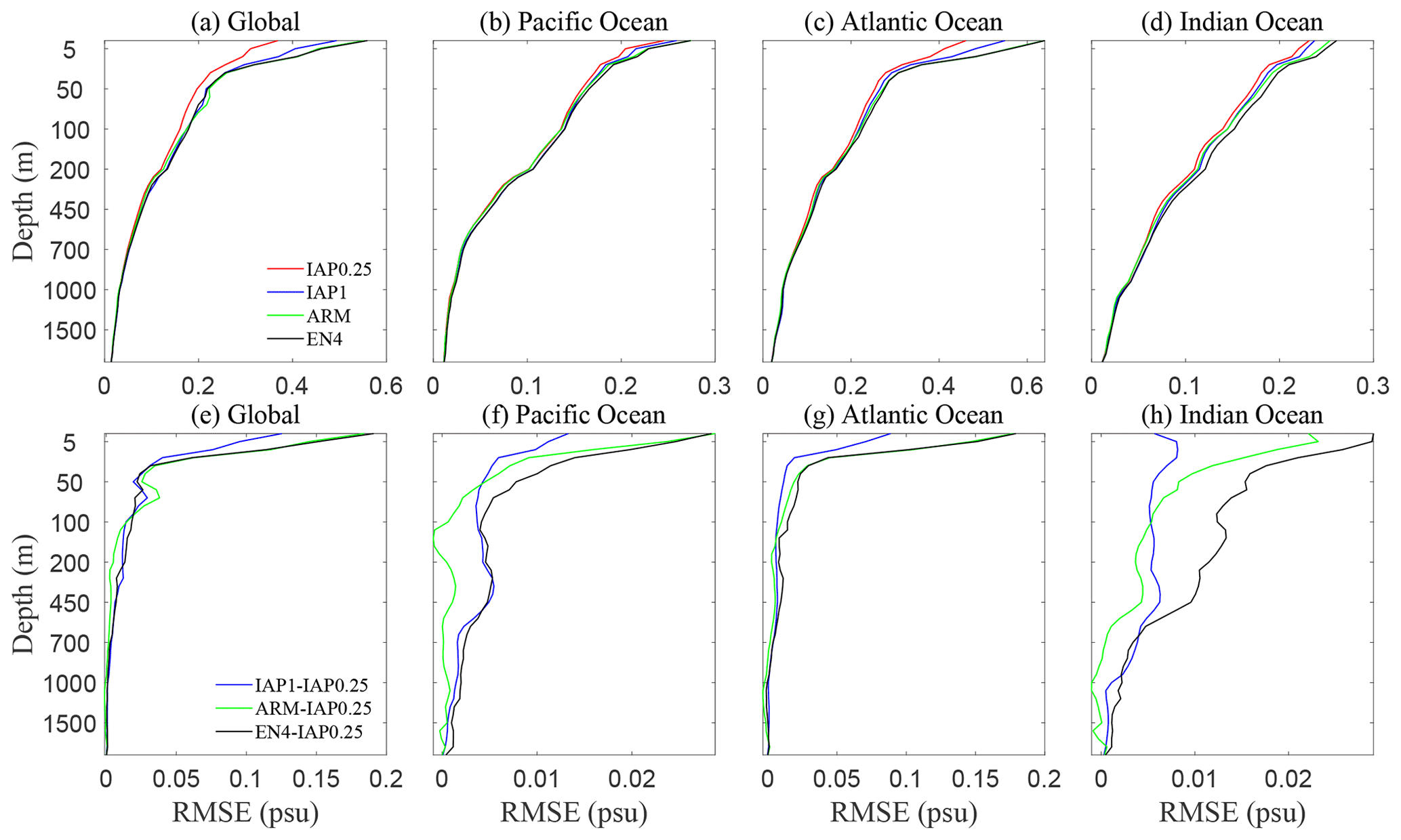
Figure 9 (a–d) Vertical distribution of RMSE for IAP1^∘, ARMOR3D, EN4, and IAP0.25^∘ for the globe and three major basin regions during 1993–2018. (e–h) Vertical distribution of RMSE for IAP1^∘, ARMOR3D, and EN4 minus IAP0.25^∘, respectively.

Table 2 RMSE of 1–2000 m mean salinity for the IAP1^∘, ARMOR3D, EN4, and IAP0.25^∘ datasets (unit: psu).

Furthermore, to identify the causes of the most significant errors, the spatial distribution of RMSE for IAP0.25^∘ and IAP1^∘ minus IAP0.25^∘ for three representative layers and 1–2000 m averages is presented in Fig. 10. Compared with IAP1^∘, the reduction in RMSE for the IAP0.25^∘ data is more dramatic in the western boundary currents, ACC region, and coastal regions (Fig. 10e–h). However, the RMSE for IAP0.25^∘ remains larger in the western boundary currents, such as the Kuroshio, Gulf Stream, and Brazil Current regions, as well as the ACC regions, compared to the open ocean. This finding is consistent with stronger mesoscale variations in these regions in the upper ocean (Frenger et al., 2015; Chassignet et al., 2020; Rhines, 2019) (Fig. 10a–d). In particular, at 5 m, IAP0.25_RMSE is larger in the Bay of Bengal and Arabian Sea, mainly because, in these areas, salinity changes are strongly affected by river runoff, surface fluxes, and ocean currents (Skliris et al., 2014; Adler et al., 2018; Liu et al., 2022). Larger errors in the ITCZ regions are also apparent at 5 and 100 m, corresponding to strong surface freshwater fluxes (Liu et al., 2022).

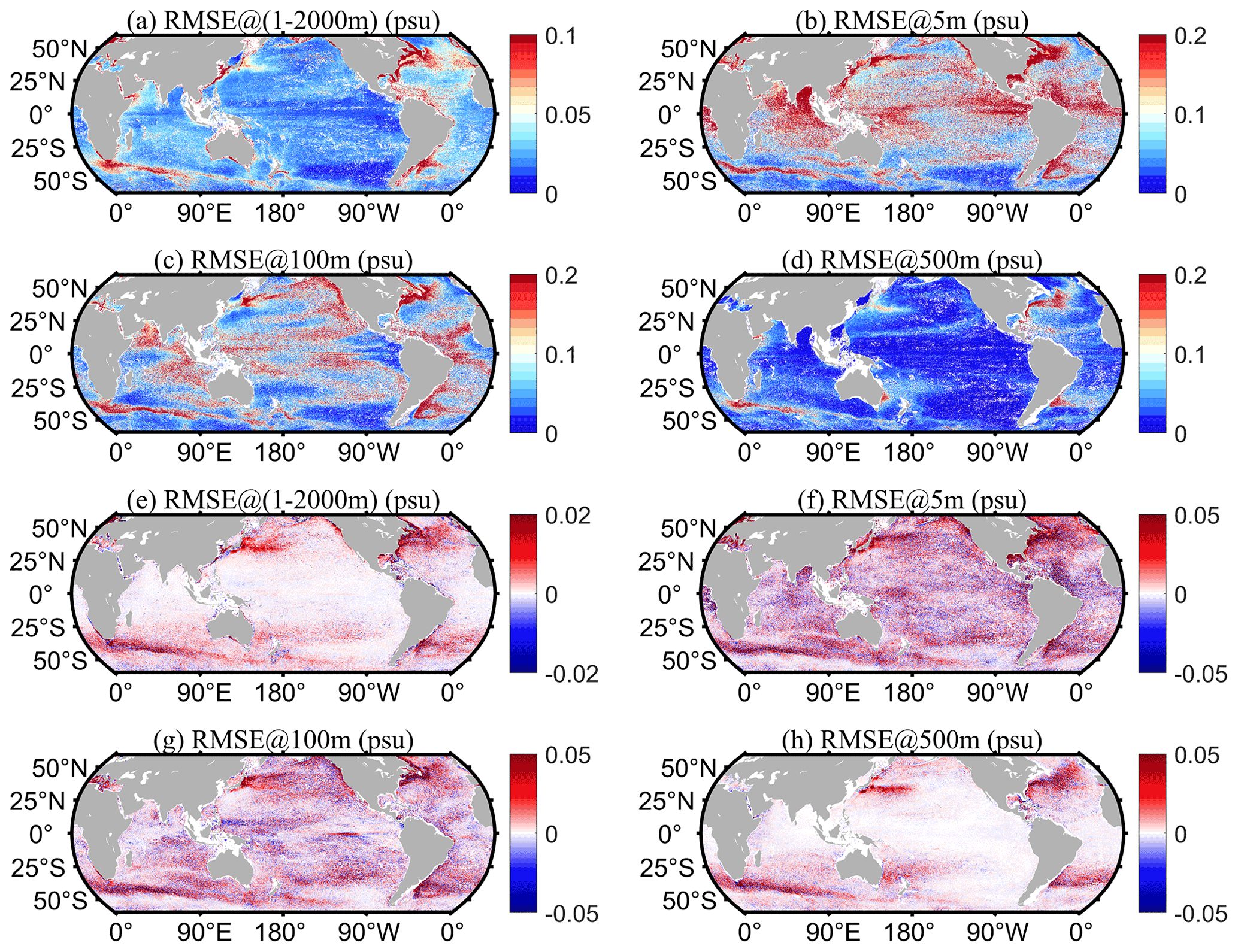
Figure 10 Geographical distribution of RMSE: (a–d) IAP0.25_RMSE and (e–h) IAP1_RMSE minus IAP0.25_RMSE.

The temporal variation of the global 1–2000 m mean RMSE from 1993 to 2018 is presented in Fig. 11 for both IAP1^∘ and IAP0.25^∘, to show the change in reconstruction performance with time. It appears that the error reduces with time, especially since the early 2000s, probably in association with there being more salinity observations available from the Argo network (Yan et al., 2021; Chen et al., 2018; Wong et al., 2020; Roemmich et al., 2019), which helps to increase the reconstruction accuracy. The RMSE has been increasing slightly in recent years, probably because of the inclusion of more real-time Argo data in our analyses. Nevertheless, IAP0.25_RMSE is smaller than IAP1_RMSE for the global ocean, by ∼11 % on average. The reduction is about 0.016 psu. The lowest RMSE reduction is seen in the Indian Ocean, likely associated with the smaller area of the western boundary current systems and relatively fewer mesoscale activities compared with the other two basins. The biggest reduction in RMSE is seen in the Atlantic Ocean (∼17 %), confirming our results in previous sections. It is interesting that there is a strong seasonal fluctuation of RMSE: it is larger in the Northern (Southern) Hemisphere summer (winter), likely because of there being fewer data in the Southern Ocean, owing to the sea-ice coverage and severe weather (Zweng et al., 2019; Gould et al., 2013; Auger et al., 2021; Durack, 2015).

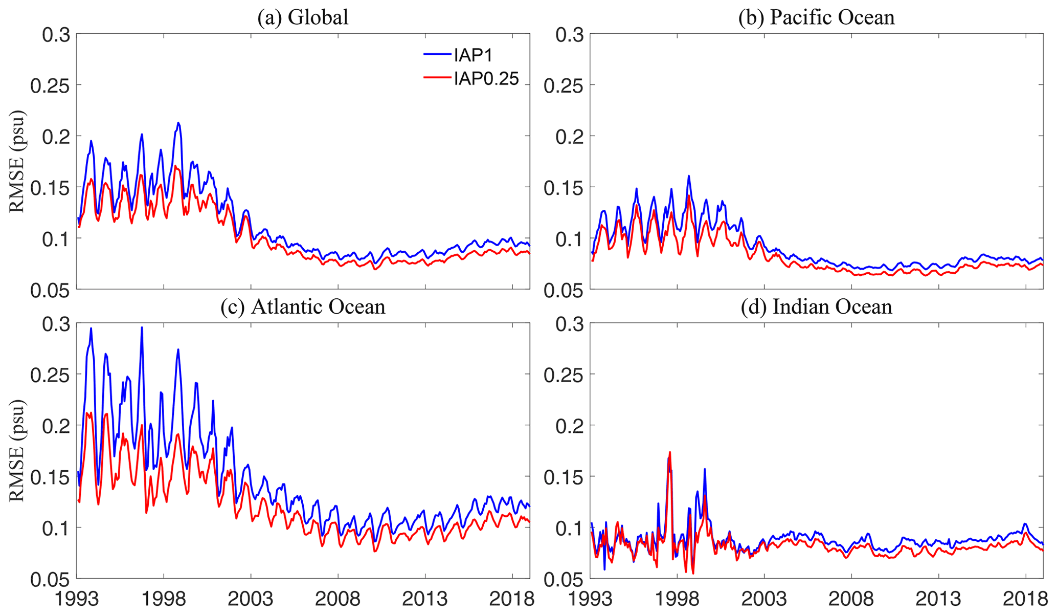
Figure 11 The 1–2000 m average RMSE time series for the IAP0.25^∘ and IAP1^∘ datasets for the globe and three ocean basins from 1993 to 2018.

In summary, statistical analysis reveals a small RMSE between the reconstruction field of IAP0.25^∘ and the in situ salinity observations, indicating an improved performance of the high-resolution reconstruction (IAP0.25^∘) in this study compared with the other products considered (IAP1^∘, ARMOR3D, and EN4). However, it should be noted here that the observations were processed by our research group and used to train the FFNN model, meaning the observations are not independent of the final reconstruction. Thus, besides the analyses reported so far, an independent validation was warranted, the results of which we report in the next section.

4 The 5-fold cross validation and uncertainty estimate

In this section, we use the results from a 5-fold cross validation to further evaluate the new reconstruction with the withheld independent observations. For this test, we trained the FFNN model with the training set (80 % of the full set) and used the withheld 20 % of data to evaluate the performance. This process was repeated five times, so the full set could be used for evaluation (i.e., the full set was divided into five sets, and each time, one set was used as the testing data, and the other four sets were training sets).

Figure 12 shows the density distribution between the reconstructed salinity value and the in situ observations for the training set (a, c) and testing set (b, d) at the depths of 10 and 100 m, separately. The diagonal line denotes a perfect reconstruction; i.e., the reconstruction perfectly matches the observations. Any errors in observations and/or reconstructions can lead to scattering of the distribution. It appears that the highest-density locations are along the diagonal line, and most of the reconstruction–observation are within ±0.2 psu for both the training and testing set, indicating that the reconstructions are obviously not biased. The density distribution for the testing set is not visibly different from the training set, suggesting that our FFNN model does not overfit the data in the training set, meaning the reconstruction method is robust in the independent data.

Additionally, we calculated the RMSE and its degradation between the reconstructed salinity fields and in situ observations of the training and testing sets at each depth layer. The degradation rate is defined as (RMSE of the testing set − RMSE of the training set) $/$ (RMSE of the training set), to quantify the generalization of the model. Figure 12a shows that RMSE of the testing set is consistent (only marginally higher than) with that of the training set. The degradation rate decreases rapidly with depth, about 5.49 % at the surface and 0.10 % at 100 m. Specifically, at 10 m, the RMSE is 0.261 psu for the training set and 0.269 psu for the testing set, and the degradation rate is 3 % (Fig. 12b and c); and at 100 m, the RMSE decreases from 0.1403 psu (training set) to 0.1401 psu (testing set) (Fig. 12d and e). Further, the correlation coefficient is slightly lower for the testing set: for example, 0.686 at 10 m but 0.707 for the training set at the same depth; at 100 m, it decreases from 0.625 (training) to 0.623 (testing). As the testing set is independent from the training set, this test indicates that the FFNN model does not experience serious overfitting, and the method is valid.

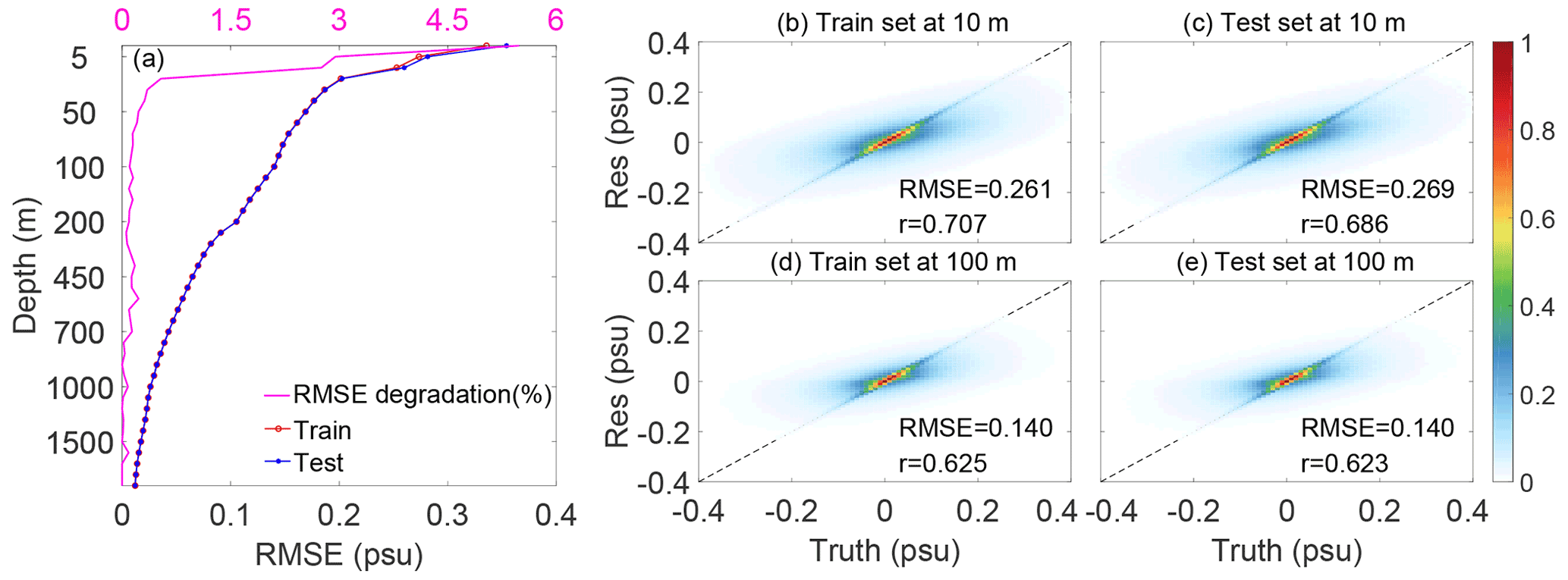
Figure 12 (a) Vertical distribution of RMSE for the training set and testing set for the global region (bottom x axis) and the RMSE degradation from the training set to the testing set (top x axis). (b–e) Density distribution diagrams at depths of 10 and 100 m for the training set and testing set, as well as RMSE and correlation coefficients (r) for the corresponding layers. The color-coded blocks represent the density of samples.

5 Evaluation of the major climatic patterns

It was shown in the previous section that IAP0.25^∘ is capable of reconstructing salinity with more mesoscale signals. However, it remains to be quantified whether the large-scale pattern of salinity change associated with climate change can be well represented in the new reconstruction. Here, we examine the long-term trends in ocean salinity using the Salinity Contrast (SC) index proposed by Cheng et al. (2020). The SC is defined as the difference between the salinity averaged over high-salinity regions (V_High, where salinity is higher than a climatological global median, S_clim) and low-salinity regions (V_Low, where salinity is below S_clim). It was calculated each month over the three-dimensional (x, y, z) ocean salinity field:

$$\begin{array}{}\text{(2)}& \mathrm{\text{SC}}\left(t\right)={\displaystyle \frac{\int \int {\int }_{V_{\mathrm{High}}}S(x,y,z,t)\mathrm{d}V}{\int \int {\int }_{V_{\mathrm{High}}}\mathrm{d}V}}-{\displaystyle \frac{\int \int {\int }_{V_{\mathrm{Low}}}S(x,y,z,t)\mathrm{d}V}{\int \int {\int }_{V_{\mathrm{Low}}}\mathrm{d}V}},\end{array}$$

where x, y, and z are the three dimensions of latitude, longitude, and depth, respectively. The terms V_High and V_Low were both determined based on the climatological salinity field.

The SC at the sea surface is called SC0; and for the 1–2000 m volume, the SC is termed SC2000. It can be seen from Fig. 13 that the IAP0.25^∘ and IAP1^∘ datasets have consistent long-term changes of SC. The global-scale SC2000 increases significantly from 1993 to 2018, with a linear trend of 0.045±0.0058 psu per century (at 90 % confidence level; the reduction of the degrees of freedom has been accounted for in this calculation). The increase of this index indicates that the phenomenon of “fresh gets fresher, salty gets saltier” is more obvious, which is mainly driven by the changes of “wet gets wetter, dry gets drier” in the global water cycle (Cheng et al., 2020; Marvel et al., 2017; Skliris et al., 2014).

Figure 13 Salinity contrast time series for IAP1^∘ and IAP0.25^∘ data in global regions from 1993 to 2018: (a) at the surface and (b) in the upper 2000 m.

Besides the global-scale SC metric, we also present the time series over the globe and in different ocean basins for IAP1^∘ and IAP0.25^∘ from 1993 to 2018 for both the salinity anomalies at the surface (S0) and averaged over the 1–2000 m volume (S2000) in Figs. 14 and 15. We divided the oceans into the Pacific Ocean (35^∘ S to 60^∘ N), Atlantic Ocean (35^∘ S to 75^∘ N), Southern Ocean (70 to 35^∘ S), North Indian Ocean (0 to 30^∘ N), and South Indian Ocean (35^∘ S to 0^∘). The uncertainty was quantified by the approach described in Sect. 2.3.3, where the ±2 standard deviation error range is provided, which corresponds to a 95 % confidence level. The two datasets continue to show high consistency.

Globally, and in the major ocean basins, IAP0.25^∘ and IAP1^∘ are consistent for S0 (Fig. 14). The S0 of both IAP1^∘ and IAP0.25^∘ shows an upward but statistically insignificant trend from 1993 to 2018. The S0 increases steadily in the Atlantic Ocean (35^∘ S–75^∘ N) and Southern Ocean (70–35^∘ S) (Fig. 14c and d). The S0 in Pacific indicates a strong decadal-scale fluctuation. In both the North and South Indian Ocean, the S0 exhibits a weak long-term decreasing trend (Fig. 14e and f).

The global mean S2000 time series (Fig. 15a) shows an increasing trend between 1993 and 2018, consistent with previous studies (Ponte et al., 2021). With more freshwater input into the ocean, the ocean salinity is expected to decrease, and thus this increase of S2000 indicates that the impact of terrestrial ice melt is difficult to resolve from salinity observations. The data drift in salinity observations is most likely responsible for the observed increase, but this issue has not been resolved yet (https://argo.ucsd.edu/faq, last access: 12 June 2022). S2000 declines steadily in the Pacific basin but increases sharply in the Atlantic basin from 1990 (Fig. 15b and c). The contrast salinity change between the Pacific Ocean (decreasing, Fig. 15b) and Atlantic Ocean (increasing, Fig. 15c) is associated with increased inter-basin transport of water vapor from the Atlantic to the Pacific (Reagan et al., 2018; Curry et al., 2003). The decadal fluctuations of S2000 in the Atlantic are greater than those in the Pacific, especially in the North Atlantic, and are in phase with the Atlantic Multidecadal Oscillation (Skliris et al., 2020; Reverdin et al., 2019). S2000 increases in the North Indian Ocean (Fig. 15e) but decreases in the South Indian Ocean (Fig. 15f), showing a “salty gets saltier, fresh gets fresher” change, mainly because of the amplified global hydrological cycle.

In summary, through our investigation of the global and basin salinity time series, we have been able to further confirm that IAP0.25^∘ can capture the integrated property of salinity changes compared with IAP1^∘. The estimated 95 % confidence intervals are generally consistent for different basins, which is about ±0.01 psu for S0 and ±0.002 psu for S2000. Although the error range of this new estimate is larger than IAP1^∘ because more sources of uncertainty are accounted for (IAP1^∘ mainly accounts for mapping and instrumental error), this new estimate could still be an underestimate because of the neglect of systematic biases (which are currently poorly known) in this study.

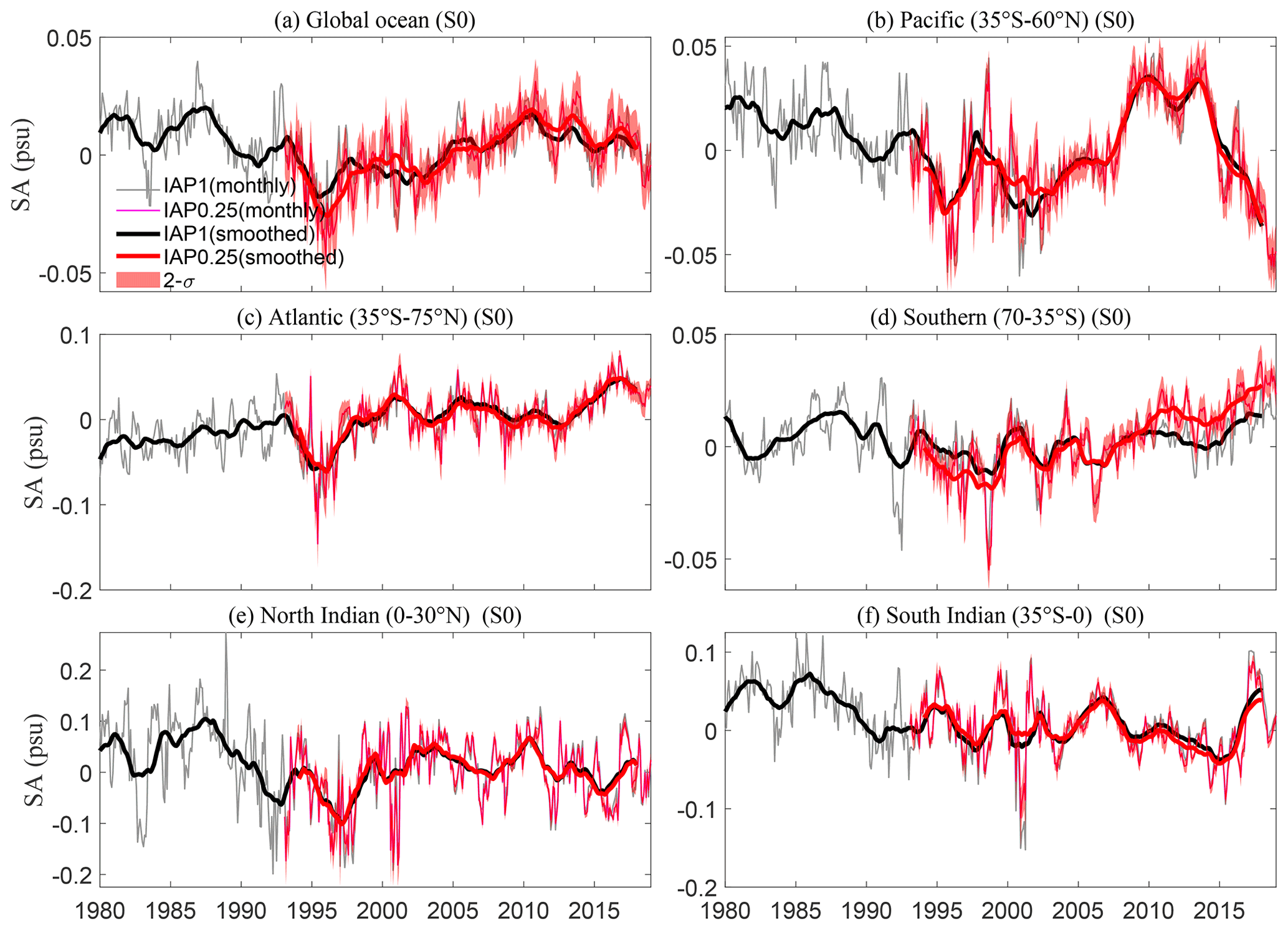
Figure 14 The global (a) and basinal (b–f) salinity anomalies (SA) time series at the surface from 1993 to 2018 for IAP1^∘ and IAP0.25^∘ respectively. Both monthly and 12-month running smoothed time series are presented; all data are relative to a 1993–2015 baseline.

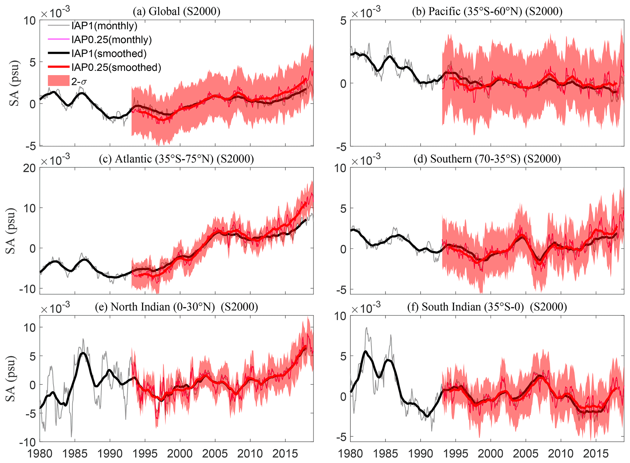
Figure 15 The global (a) and basinal (b–f) 1–2000 m averaged salinity anomalies (SA) time series from 1993 to 2018 for IAP1^∘ and IAP0.25^∘ respectively. Both monthly and 12-month running smoothed time series are presented; all data are relative to a 1993–2015 baseline.

6 Importance of each feature for the reconstruction

The impact of different inputs on the reconstruction of IAP0.25^∘ using the FFNN model is shown in Fig. 16 using the SHAP method. At the surface (Fig. 16a and c), the location parameters (latitude, longitude, and depth) are the most important inputs and are probably linked to the strong spatial variability of salinity near sea surface. The IAP1^∘ plays a secondary role near the surface because it provides direct information of salinity and represents the large-scale salinity changes. Accumulatively, the remote-sensing data contribute to ∼20 % of the reconstruction. For the subsurface (Fig. 16c), IAP1^∘ plays a more important role than that near the surface (∼26 % for 1–2000 m average; Fig. 16b), and this is physically meaningful because there is less mesoscale variability in the deeper ocean, and large-scale variability becomes more important at the sea subsurface. ADTA becomes more important within 100–700 m than the other layers because both salinity and ADTA are strongly associated with thermocline variations. VSSWA, USSWA, and SSTA play similar roles from the surface to 2000 m (<5 % for each) and are smaller than most of the other inputs, probably because their changes are only weakly coupled with salinity compared with other parameters. It is interesting that time information (<3 %) plays the smallest role in reconstruction, implying that the FFNN can be applied in other time periods without losing too much accuracy.

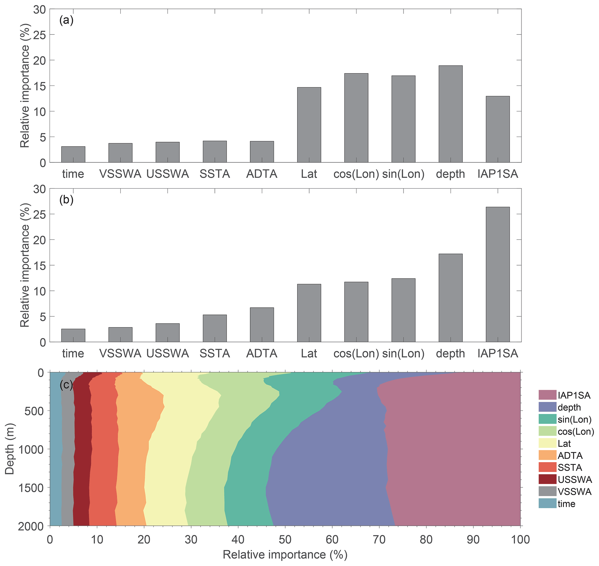
Figure 16 A quantification of the relative importance of each input in reconstruction of IAP0.25^∘: (a) at the surface, (b) 1–2000 m average, and (c) at each depth from 1 to 2000 m. The input features are ranked in terms of importance; i.e., the higher the SHAP value is, the more important the features are.

7 Data availability

The code used in this paper includes data processing, optimal model building and the result prediction. The reconstructed IAP0.25^∘ dataset is available at https://doi.org/10.57760/sciencedb.o00122.00001 (Tian et al., 2022) or http://www.ocean.iap.ac.cn/ftp/cheng/IAP_v0_Ocean_Salinity_0p25_FFNN_0_2000m/ (last access: 4 October 2022). Here we provide global ocean salinity gridded product at 0.25^∘ × 0.25^∘ horizontal resolution on 41 vertical levels from 1–2000 m and at a monthly resolution from 1993 to 2018.

8 Summary and discussion

This study used an FFNN approach to reconstruct a high-resolution (0.25^∘ × 0.25^∘) ocean subsurface salinity dataset (1–2000 m) for the period 1993–2018, in which the spatial and temporal information (time, longitude, latitude, and depth), previously available the 1^∘ × 1^∘ resolution salinity dataset, and satellite remote-sensing data (ADT, SST, SSW) were given as inputs to the FFNN algorithm for reconstruction. By training the functional relationship between input variables and truth values (observed gridded averaged salinity), the reconstruction model was established. For the IAP0.25^∘ salinity data, the global and regional reconstruction performance was evaluated using several different tests. In brief, we show that (1) IAP0.25^∘ salinity data maintain the large-scale information from IAP1^∘ gridded data. Because previous evaluations suggest that IAP1^∘ provides more physically tenable large-scale patterns and long-term climate change and variabilities compared to many available datasets (Cheng et al., 2020; Reed et al., 2022; Sohail et al., 2022), the reliability of large-scale signals also becomes an advantage of the new IAP0.25^∘ product. (2) Compared with IAP1^∘, the RMSE of IAP0.25^∘ can be reduced by ∼11 % on a global average. In addition, IAP0.25^∘ shows more realistic spatial signals in the Gulf Stream, Kuroshio, and Antarctic Circumpolar Current regions, with stronger mesoscale variations than the IAP1^∘ product, indicating that FFNN can effectively transfer small-scale spatial variations in ADT, SST, and SSW fields into the 0.25^∘ × 0.25^∘ salinity field. It thus serves as an improvement on the currently available IAP data. (3) We show that the FFNN approach is effective in merging different kinds of Earth observations, and the method is robust and can be reliably used for ocean state reconstruction; thus it can complement the existing data assimilation and objective analysis methods.

Although the validity and advantages of the FFNN approach have been demonstrated, there are some caveats and limitations to this approach, related to which we provide some future guidance. This study used a probabilistic approach to quantify the uncertainty, which is a practical strategy, and with this approach all major error sources are propagated to the final fields. However, uncertainty assessment with machine learning is still a challenge for many available products, and this issue requires future analysis: i.e., how sensitive the FFNN approach is to parameter choices such as the number of hidden layers and neurons.

Compared with the ARMOR3D data, it seems that the small-scale signals are weaker in IAP0.25^∘ (for example Figs. 5 and 6), indicating a difference of efficiency with which signals of the remote-sensing data are transmitted into the salinity reconstruction. Therefore, an intriguing scientific question is the following: what is the key factor determining the efficiency? Addressing this question requires a dedicated study that incorporates an intercomparison among other approaches.

As a coarse-resolution product, IAP1^∘ is important in high-resolution reconstructions and provides a critical large-scale precondition. The uncertainty (or biases) in this coarse-resolution field will propagate into the reconstruction, but how the uncertainty propagates and contributes to the final estimate is still an open question. One of the aims of this study was to ensure the continuity from IAP1^∘ to IAP0.25^∘ data because work has already shown superiority of IAP1^∘ in large-scale reconstructions compared with many available datasets (Cheng et al., 2020). Thus, this study further advances the prior findings of Cheng et al. (2020). Further experiments are needed to quantify the sensitivity of the results to this preconditioning.