HMRFS–TP: long-term daily gap-free snow cover products over the Tibetan Plateau from 2002 to 2021 based on hidden Markov random field model

Snow cover plays an essential role in climate change and the hydrological cycle of the Tibetan Plateau. The widely used Moderate Resolution Imaging Spectroradiometer (MODIS) snow products have two major issues: massive data gaps due to frequent clouds and relatively low estimate accuracy of snow cover due to complex terrain in this region. Here we generate long-term daily gap-free snow cover products over the Tibetan Plateau at 500 m resolution by applying a hidden Markov random field (HMRF) technique to the original MODIS snow products over the past two decades. The data gaps of the original MODIS snow products were fully filled by optimally integrating spectral, spatiotemporal, and environmental information within HMRF framework. The snow cover estimate accuracy was greatly increased by incorporating the spatiotemporal variations of solar radiation due to surface topography and sun elevation angle as the environmental contextual information in HMRF-based snow cover estimation. We evaluated our snow products, and the accuracy is 98.29 % in comparison with in situ observations, and 91.36 % in comparison with high-resolution snow maps derived from Landsat images. Our evaluation also suggests that the incorporation of spatiotemporal solar radiation as the environmental contextual information in HMRF modeling, instead of the simple use of surface elevation as the environmental contextual information, results in the accuracy of the snow products increases by 2.71 % and the omission error decreases by 3.59 %. The accuracy of our snow products is especially improved during snow transitional period, and over complex terrains with high elevation and sunny slopes. The new products can provide long-term and spatiotemporally continuous information of snow cover distribution, which is critical for understanding the processes of snow accumulation and melting, analyzing its impact on climate change, and facilitating water resource management in Tibetan Plateau. This dataset can be freely accessed from the National Tibetan Plateau Data Center at https://doi.org/10.11888/Cryos.tpdc.272204 (Huang and Xu, 2022).

1 Introduction

Snow cover has the characteristics of low thermal diffusivity, high reflectivity, and strong water storage capacity, which has a profound effect on climate change (Gao et al., 2012), radiation budget (Yang et al., 2014; Huang et al., 2019), hydrological cycle (Dong, 2018), and human activities (Cereceda-Balic et al., 2020). The Tibetan Plateau (TP) has abundant snow cover, with highest elevation and largest snow cover area in the middle latitudes of the Northern Hemisphere (Qiu, 2008; Yao et al., 2019). Snow is highly sensitive to climate change (Chen et al., 2018a), and snowmelt water quantity is closely connected to the supply of soil moisture on the plateau (Wang et al., 2018) and the runoff of numerous rivers such as the Yangtze and Yellow rivers (Immerzeel et al., 2010). Long-term and detailed snow cover information is fundamental to investigating climate change and hydrological cycle of the TP.

Remote sensing has allowed extraction of historical and near-real-time snow cover extent over inaccessible areas (Yang et al., 2015; Li et al., 2018). Snow products could be acquired via remote sensing satellites, such as the Landsat and Sentinel-2 series. Although these satellites have a high spatial resolution, they have a relatively coarse (10 or 16 d) temporal resolution, thereby rendering them insufficient to monitor the temporal variations in snow cover (Huang et al., 2022). Moderate Resolution Imaging Spectroradiometer (MODIS) has commenced producing snow products at 500 m resolution from 2000, which have been widely utilized as the primary datasets for monitoring snow cover (Muhammad and Thapa, 2020; Kilpys et al., 2020). The accuracy of MODIS snow products is greater than 85 % at the global scale under clear sky (e.g., Parajka et al., 2012; Yang et al., 2015). However, these products have many data gaps due to frequent clouds, causing discontinuity in the time and space of the products (Y. Liu et al., 2020​​​​​​​). In addition, the complex terrain of the TP makes it more challenging for accurate snow cover detection. Previous studies (Dong and Menzel, 2016; Dariane et al., 2017) have suggested the low accuracy of MODIS snow products for mountainous areas.

Various data-gap-filling techniques have been proposed to produce seamless MODIS snow cover products including multi-source combination, temporal, spatial, and spatiotemporal filters (Xiao et al., 2021; Hussainzada et al., 2021; Richiardi et al., 2021). The multi-source combination method combines MODIS with passive microwave sensor data (Y. Li et al., 2019; Li et al., 2020). Although this method can be used to fill most data gaps, the accuracy of the combined product depends more on the accuracy of the microwave sensor data, and the spatial resolution (>1 km) is not sufficient to meet the demands for accurately assessing the snow cover variability (Wang et al., 2009). Many attempts have been directed toward filling the gaps in MODIS optical remote sensing data based on spatial and temporal information. Temporal methods are used to reclassify the data-gap pixels by inferring the land cover types of the current pixels under clear sky within a few days before or after (e.g., the previous or next day) (X. Li et al., 2019; Tran et al., 2019). Spatial methods estimate data-gap pixels based on gap-free pixels in the spatial neighborhood (Hou et al., 2019). Relevant environmental information (e.g., snow lines and topography) has been introduced into spatial methods (Wang et al., 2019; Kilpys et al., 2020). Spatiotemporal methods have been integrated to fill as many data gaps as possible (Parajka and Blöschl, 2008; Kilpys et al., 2020). These studies integrated all information (i.e., spatiotemporal, and environmental information) according to heuristic rules instead of rigorous quantitative models. Huang et al. (2018) developed a hidden Markov random field (HMRF) framework to optimally combine all information. This technique not only fills data gaps but also provides fine improvement in accuracy compared to the original MODIS snow products.

The long-term series and high-precision products are the basis for snow cover research on the TP, which enable the monitoring and analysis of snow cover phenology and more comprehensive understanding of the snow cover trend. However, the existing daily products for the TP have an earlier end date (the latest version at 500 m resolution product ended in 2015), and some products still have a small number of data gaps (Yu et al., 2016; Xu et al., 2017; Zheng and Cao, 2019). Thus, long-term and high-precision daily snow cover products for the TP should be generated using reliable data-gap-filling methods.

Here we generate long-term daily snow cover products over the TP by applying an HMRF technique (Huang et al., 2018) to the original MODIS snow products from 2002 to 2021. In the previous HMRF modeling technique (Huang et al., 2018), surface elevation was considered as a surrogate for environmental information in mountainous regions. However, according to in situ photos from field survey in the TP, we found that the distribution of snow cover differed from the model results, even at the same elevation level (Fig. 1b and c). The snow on the TP is strongly infected by complex topography (e.g., slope, aspect, sunlight duration, and solar incidence angle). Thus, while generating our new snow cover product, we incorporated solar radiation as a comprehensive indicator of topographical effects to correct the snow identification errors caused by the complex terrain of the TP.

Our study is outlined as follows: first, we present our study area and datasets. Then, we present the HMRF framework and data-processing flowchart. By employing this modeling technique to the TP, we produced daily gap-free snow cover products for the TP from 2002 to 2021. We also validated our new snow products against in situ observations, snow cover mapped from Landsat series data, and snow cover data estimated from the initial MODIS and original HMRF modeling technique.

2 Study area and data

2.1 Study area

The TP is situated in western China, spanning 26^∘00^′–39^∘46^′ N and 73^∘18^′–104^∘46^′ E (Fig. 1). It encompasses approximately 2.56 ×10⁶ km², with an average altitude exceeding 4000 m, and is one of the most susceptible regions to climate change (Jing et al., 2019). The air temperature in the TP increased from the northwest to southeast, with more precipitation in the southeast and less in the northwest (Wang et al., 2018). Generally, the TP has comparatively low temperatures and has largest distribution of glaciers and snow in China (Liang et al., 2017). Seasonal snow cover on the TP has a great potential to influence the hydrological cycle and heat wave frequency in northern China (Wu et al., 2012). In addition, seasonal snow accumulation on the TP is an important part of surface water accumulation in southwestern China and surrounding countries. Several major rivers in China and surrounding Asian countries, such as the Yangtze, Yellow, Mekong, Salween, Brahmaputra, Ganges, and Indus rivers, all originate from the TP.

The status of the snow in the TP changes rapidly as a result of multiple factors, such as temperature, precipitation, synoptic forcing, and large-scale ocean–atmosphere oscillations (You et al., 2020), which may lead to sublimation and snowfall (Li et al., 2020). Affected by the Indian Ocean monsoon and East Asian summer monsoon, the southeast TP has plenty water vapor, which results in a large amount of cloud, particularly in spring and summer (Yang et al., 2015).

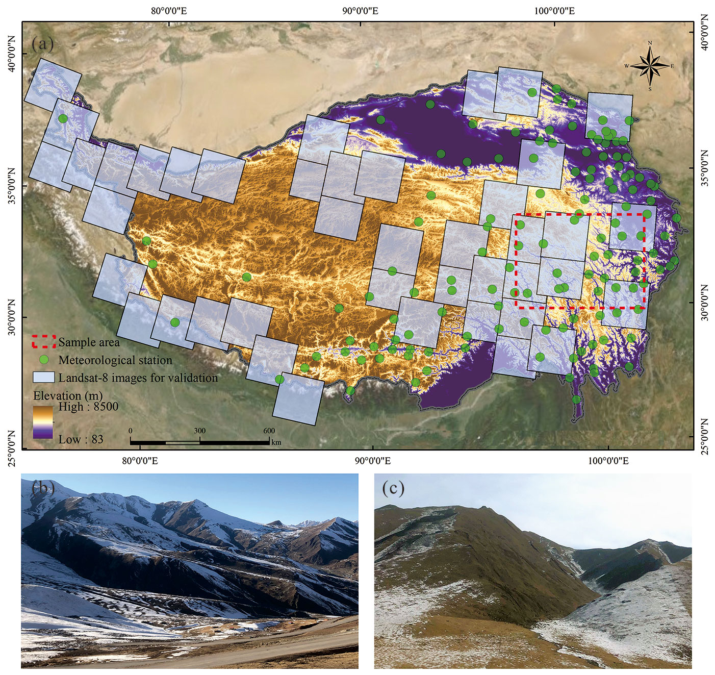
Figure 1 Topography, meteorological stations, and survey photos of the TP. (a) Surface elevation and distribution of meteorological stations in the TP. Landsat images utilized for validation and sample area are also shown; (b) and (c) in situ photos from field survey in the TP.

2.2 Datasets

2.2.1 Daily MODIS snow cover products

We used version six MODIS daily snow products on Terra (MOD10A1 v6) and Aqua (MYD10A1 v6) from 15 May 2002 to 31 December 2021 (Hall and Riggs, 2016a, b). Google Earth Engine (GEE) (https://earthengine.google.com, last access: 20 January 2022) platform was used for pre-processing the MODIS snow product. We used MODIS/006/MOD10A1 and MODIS/006/MYD10A1 datasets and NDSI_Snow_Cover and NDSI_Snow_Cover_Class bands. NDSI_Snow_Cover represents the value of the normalized difference snow index (NDSI), ranging 0–100. The values in the NDSI_Snow_Cover_Class band include 200, 201, 211, 237, 239, 250, 254, and 255, which represent “missing data”, “no decision”, “night time”, “inland water”, “ocean”, “clouds”, “detector saturated”, and “filled data”, respectively (Riggs et al., 2019).

The original NDSI data were reclassified as snow, non-snow, and data-gaps classes (Chen et al., 2020; Huang et al., 2018, 2022). The pixels with an NDSI value of 40–100 in the NDSI_Snow_Cover band were reclassified as snow (Riggs et al., 2017). The pixels with an NDSI value of 0–40 in the NDSI_Snow_Cover band and with corresponding values of 237 and 239 in the NDSI_Snow_Cover_Class band were reclassified as non-snow. The remaining pixels were reclassified as data gaps. Then, we combined the MOD10A1 and MYD10A1 reclassification results of the same day according to the following rules: when a pixel included gap-free data in both MOD10A1 and MYD10A1 products, value in the MOD10A1 product was used; when a pixel included gap free only in the one product, the gap-free data value was used. Finally, the combined Terra and Aqua results were re-projected onto Universal Transverse Mercator (UTM zone 45) at 500 m resolution, which was used as the initial snow cover products for filling data gaps in this research.

We identified the data gaps in original composite MODIS products, and found the annual average data gap proportion of the TP was 33.63 %–38.75 %, with an average of 36.12 % (Fig. 2). The monthly average data gaps are also shown in Fig. 2, and we found that the data gaps of the TP were the largest in summer (June to August), with an average of 45.20 %. The data gaps declined rapidly starting from September and were the smallest in November (with an average of 28.00 %), and gradually increased in winter and spring.

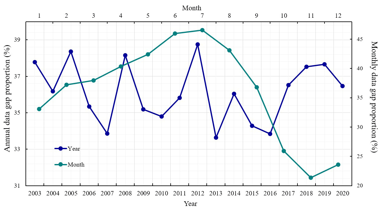
Figure 2 Annual and monthly average proportion of data gaps of original composite MODIS snow products.

2.2.2 Digital Elevation Models (DEMs)

We used the Shuttle Radar Topography Mission (SRTM) DEMs to calculate the topographical parameters (e.g., elevation, slope, and aspect). The SRTM DEM at 90 m resolution in GeoTIFF format was from the United States Geological Survey (USGS). We then pre-processed the DEM data, including mosaicking, reprojection, resampling, and clipping.

2.2.3 In situ observations

We used snow depths from 137 in situ stations in the TP (Fig. 1a) obtained from 1 October 2002 to 31 March 2021, which were provided by the National Meteorological Centre of China. Figure 1a shows all stations over the TP, which record coordinates, observation time, snow depth, and snow pressure. The surface elevation of these stations ranges from 1187 to 5310 m, with an average of 3240 m. Overall, 72 % stations are situated in the east (>95^∘ E), and only 22 % are situated in high-altitude areas (>4000 m). A 3 cm threshold was utilized to evaluate the snow classes using in situ snow depth (Huang et al., 2022). The snow depth was reclassified as no-snow if it was less than 3 cm; if not, it was considered as snow.

2.2.4 Landsat images

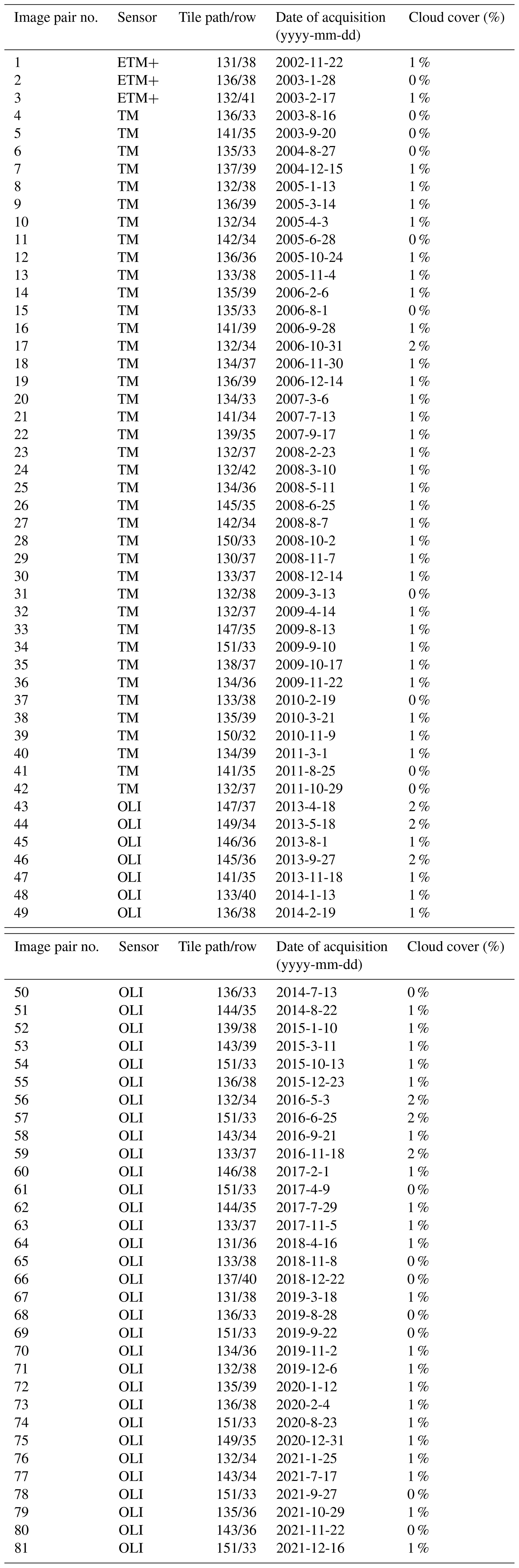
The snow cover mapped from Landsat images were used to validate and evaluate our snow cover product. Using the GEE cloud platform, we selected 81 Landsat series images with less than 2 % cloud coverage under clear sky for verification, including Landsat-5 TM, Landsat-7 ETM+, and Landsat-8 OLI images. The detailed Landsat images information is shown in the supplementary material (Table A1). The selected images were distributed throughout the study area from 22 November 2002 to 16 December 2021. We used the C topographic correction model to correct for the terrain effect on Landsat series data (Teilet et al., 1982). Then, using the SNOWMAP method proposed by Hall et al. (1995), we generated a snow cover map using Landsat images for the TP. The SNOWMAP algorithm classified the pixels with NDSI values >0.4, green band >0.10, and shortwave infrared band >0.11 as snow (Huang et al., 2011). To improve the accuracy of resampling 30 to 500 m resolution, we adopted the following steps for resampling: first, for each MODIS pixel, we calculated the amount of Landsat snow-covered pixels in the current MODIS pixel. Second, we divided the snow-covered Landsat pixels by the sum of the Landsat pixels contained in each MODIS pixel (a 500 m MODIS pixel is close to 277 Landsat pixels) (Crawford, 2015; C. Liu et al., 2020). Finally, we reclassified pixels whose results in the previous step were less than 0.5 as no-snow; otherwise, they were reclassified as snow. Hence, we obtained resampled 500 m resolution Landsat images for further verification.

3 HMRF modeling technique

The HMRF framework optimally combines MODIS spectral, spatiotemporal, and environmental information to fill data gaps, thereby increasing snow estimate accuracy (Huang et al., 2018). This framework is expressed as a linear energy function in which the total energy is modeled as the combination of all information (Eq. 1). Thus, the HMRF framework requires to specify energy function for each information and to determine the optimal parameters that minimize the total energy.

$$\begin{array}{}\text{(1)}& \begin{array}{rl}{U}_T& \left({\mathit{\beta }}_n,x_i,N_{\mathrm{sp}},N_{\mathrm{tp}},I_{\mathrm{ev}}\right)={\mathit{\lambda }}_{xi}{U}_{xi}\left({\mathit{\beta }}_n,x_i\right)\\ & +{\mathit{\lambda }}_{\mathrm{st}}{U}_{\mathrm{st}}\left({\mathit{\beta }}_n,N_{\mathrm{sp}},N_{\mathrm{tp}}\right)+{\mathit{\lambda }}_{\mathrm{ev}}{U}_{\mathrm{ev}}\left({\mathit{\beta }}_n,I_{\mathrm{ev}}\right),\end{array}\end{array}$$

where λ_xi, λ_st, and λ_ev are the spectral, spatiotemporal, and environmental parameters, respectively; and U_xi, U_st, and U_ev are the spectral, spatiotemporal, and environmental energy functions, respectively.

In the original HMRF modeling technique, Huang et al. (2018) used surface elevation to represent the environmental association in mountainous areas (hereafter referred to as HMRF_ele). However, because of the spatial heterogeneity of the TP, using only relative elevation cannot reflect the influence of complex terrain on snow cover (Fig. 1b and c). Therefore, the influence of additional topographic factors (e.g., slope, aspect, sunlight duration, and solar incidence angle) on snow cover must be considered. Based on the above reasons, we incorporated solar radiation as a surrogate for environmental information in HMRF framework (hereafter referred to as HMRF_solar). Further details are provided in Sect. 3.3.

The overall flowchart of the HMRF_solar modeling technique is shown in Fig. 3. We used daily composite MODIS snow cover products as the initial dataset. First, we calculated the optimal parameters of each information using the Ho-Kashyap and DFBETAS algorithms (Bormann et al., 2012), based on randomly divided training samples on the initial snow cover product. Second, we determined the snow and non-snow classes of each pixel in the initial snow cover products using the optimal parameters and HMRF_solar algorithm. In the first round of the HMRF_solar algorithm, we employed a $\mathrm{3}\times \mathrm{3}\times \mathrm{3}$ spatiotemporal cubic neighborhood to model spatiotemporal energy. If data gaps remained, we further expanded the cubic neighborhood of these pixels. Finally, we validated and evaluated our HMRF_solar-based products against the in situ observations, snow mapped from Landsat images, and snow cover data from the initial MODIS and original HMRF_ele modeling technique.

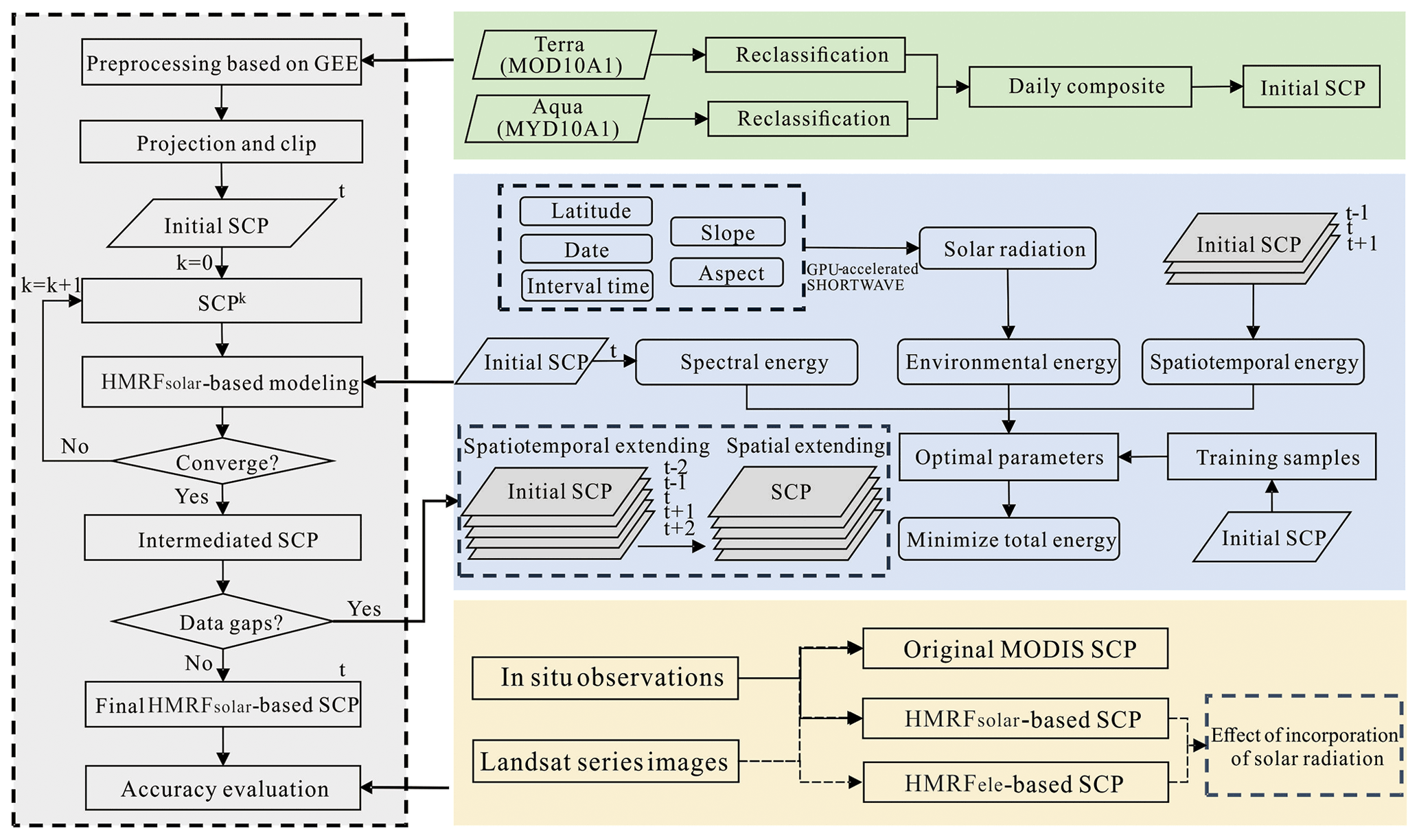
Figure 3 Overall flowchart of the HMRF_solar-based framework. (SCP stands for snow cover products.)

3.1 Spectral information

The spectral energy is considered as the possibility of the pixel pertaining to non-snow or snow according to its spectral information. Fractional snow cover (FSC) represents the proportion of snow in a pixel, which can be calculated using the NDSI value provided by the MODIS snow product (Salomonson and Appel, 2004). The general linear relationship between FSC and NDSI was derived over other regions, which has limited accuracy in the TP. Therefore, we re-fitted that empirical relationship of Terra and Aqua satellites in the TP using Landsat data over 20 years with 972 884 and 952 221 sample points, respectively. The spectral probability P(x_i | β₁) of snow class was re-fitted as follows:

$$\begin{array}{}\text{(2)}& {\displaystyle }P{\left(x_i|{\mathit{\beta }}_{\mathrm{1}}\right)}_{\mathrm{Terra}}=(\mathrm{1.222}\times \mathrm{NDSI}+\mathrm{0.038})/\mathrm{100}\text{(3)}& {\displaystyle }P{\left(x_i|{\mathit{\beta }}_{\mathrm{1}}\right)}_{\mathrm{Aqua}}=(\mathrm{1.164}\times \mathrm{NDSI}+\mathrm{0.058})/\mathrm{100}.\end{array}$$

The correlation coefficients of the re-fitted equation of Terra and Aqua satellites were 0.86 and 0.89, respectively. The spectral energy U_xi(β_n,x_i) can be calculated as follows:

$$\begin{array}{}\text{(4)}& U_{xi}\left({\mathit{\beta }}_n,x_i\right)\left\{\begin{array}{l}-\left[P\left(x_i|{\mathit{\beta }}_{\mathrm{1}}\right)\right],\text{if}n=\mathrm{1}\\ -[\mathrm{1}-\left[P\left(x_i|{\mathit{\beta }}_{\mathrm{1}}\right)\right],\text{if}n=\mathrm{2}\end{array}\right.,\end{array}$$

where if pixel i is classified as no-snow class, then n=2; if pixel i is the snow class, n=1.

3.2 Spatiotemporal information

To fully take advantage of spatiotemporal information, we combined the temporal and spatial information to form a spatiotemporal cubic neighborhood N_st (Huang et al., 2018). In modeling, initial snow products are updated iteratively using classification results from the previous iteration. Convergence ends when the proportion of pixels whose type changes between two subsequent iterations is less than 0.1 %, in which case the data gaps need to be calculated. If the data gaps still exist, the cubic neighborhood is temporally and spatially expanded in the next round.

We primarily set a $\mathrm{3}\times \mathrm{3}\times \mathrm{3}$ cubic neighborhood; that is, the current pixel and its neighboring pixels formed a cube on day t, the day before (t−1), and the day after (t+1). In this condition, the energy equation of the current pixel is expressed as the weight of the proportion of snow and non-snow in the spatiotemporal neighborhood of the current pixel. The weight is reversely proportional to the distance from the neighboring pixel to the center pixel:

$$\begin{array}{}\text{(5)}& U_{\mathrm{st}}\left({\mathit{\beta }}_n,N_{\mathrm{sp}},N_{\mathrm{tp}}\right)=\left\{\begin{array}{l}-{\sum }_{x=-\mathrm{1}}^{\mathrm{1}}{\sum }_{y=-\mathrm{1}}^{\mathrm{1}}{\sum }_{t=-\mathrm{1}}^{\mathrm{1}}\frac{\frac{S(x,y,t)}{\mathrm{Dist}(x,y,t)}}{\frac{V(x,y,t)}{\mathrm{Dist}(x,y,t)}},\\ \text{if}n=\mathrm{1}\\ -{\sum }_{x=-\mathrm{1}}^{\mathrm{1}}{\sum }_{y=-\mathrm{1}}^{\mathrm{1}}{\sum }_{t=-\mathrm{1}}^{\mathrm{1}}\frac{\frac{\mathrm{NS}(x,y,t)}{\mathrm{Dist}(x,y,t)}}{\frac{V(x,y,t)}{\mathrm{Dist}(x,y,t)}},\\ \text{if}n=\mathrm{2}\end{array}\right.,\end{array}$$

where $(x,y,t)$ is the relative coordinates of the pixel in the spatiotemporal cube; $S(x,y,t$), $\mathrm{NS}(x,y,t$), $V(x,y,t$), and $\mathrm{Dist}(x,y,t$) are defined respectively as follows:

$$\begin{array}{}\text{(6)}& {\displaystyle }S\left(x,y,t\right)=\left\{\begin{array}{l}\mathrm{1},\text{if}\left(x,y,t\right)\text{pertains to snow}\\ \mathrm{0},\text{if}\left(x,y,t\right)\text{pertains to non-snow}\end{array}\right.\text{(7)}& {\displaystyle }\mathrm{NS}\left(x,y,t\right)=\left\{\begin{array}{l}\mathrm{1},\text{if}\left(x,y,t\right)\text{pertains to non-snow}\\ \mathrm{0},\text{if}\left(x,y,t\right)\text{pertains to snow}\end{array}\right.\text{(8)}& {\displaystyle }V\left(x,y,t\right)=\left\{\begin{array}{l}\mathrm{1},\mathrm{if}\left(x,y,t\right)\text{pertains to valid class}\\ \mathrm{0},\text{if}\left(x,y,t\right)\text{pertains to data gaps}\end{array}\right.\text{(9)}& {\displaystyle }\mathrm{Dist}\left(x,y,t\right)=\sqrt{x^{\mathrm{2}}+y^{\mathrm{2}}+w{t}^{\mathrm{2}}},\end{array}$$

where $\mathrm{Dist}\left(x,y,t\right)$ is the distance from each neighborhood pixel to the center pixel, which determines the weight of each area pixel; w denotes the weight of the temporal distance related to the spatial distance. This value was calculated via semi-variogram analysis and was determined as 3 in this study.

If data gaps still remain in $\mathrm{3}\times \mathrm{3}\times \mathrm{3}$ spatiotemporal cubic neighborhood, we further expanded spatiotemporal neighborhood to $\mathrm{5}\times \mathrm{5}\times \mathrm{5}$. In this study, when we used a $\mathrm{5}\times \mathrm{5}\times \mathrm{5}$ cubic neighborhood, the data gaps were reduced to 0.0173 %, which had little effect on snow cover estimate accuracy. Hence, the temporal neighborhood remained at 5, whereas the spatial neighborhood continued to expand. Finally, all data gaps could all be filled by continuously expanding the spatial neighborhood, which remarkably improved the MODIS estimate accuracy.

3.3 Environmental contextual information

The geographic location and seasons can determine the total solar radiation received on the TP, and the complex topography of the TP determines the availability of solar radiation at specific locations in the region, which further affects accumulation and melting of snow cover and determines its distribution (You et al., 2020). Here we use solar radiation to include the influence of environmental factors on snow cover, such as slope, aspect, sunlight duration, and solar incidence angle.

Kumar et al. (1997) originally proposed the solar radiation model, SHORTWAVE, to calculate the direct, reflected, and diffuse solar energy received by the ground. Huang et al. (2015) used a graphics processing unit (GPU) methodology to improve the speed and effectiveness for modeling. In our study, we used the GPU-accelerated SHORTWAVE model as the environmental parameter in the HMRF_solar model to calculate the daily solar radiation of the TP.

A general-purpose desktop computer was used to test the parallel computational efficiency. The computer has an Intel Core™ i7-10700 CPU (16 cores and max clock rate is at 2.90 GHz), an NVIDIA GeForce RTX 2070 SUPER card with 2560 cores and 16 240 MB global memory, and Windows 11 Ultimate 64 bit operation system. The GPU-accelerated SHORTWAVE model uses latitude, slope, aspect, date, and interval time as inputs. To calculate the overall solar radiation in a day, we subdivided the day into subsequent time intervals, and set 15 min as the suitable interval time in this paper (Kumar et al., 1997; Antonic, 1998). The overall solar radiation I_a at time t can be calculated using Eq. (10),

$$\begin{array}{}\text{(10)}& I_{\mathrm{a}}=I_{\mathrm{p}}+I_{\mathrm{d}}+I_{\mathrm{r}},\end{array}$$

where I_p, I_d, and I_r are the direct, diffuse, and reflected solar radiation, respectively, and can be estimated using the following equations:

$$\begin{array}{}\text{(11)}& {\displaystyle }{I}_{\mathrm{p}}=I_{\mathrm{0}}\cdot {\mathit{\tau }}_{\mathrm{b}}\cdot \cos \mathit{\theta }\text{(12)}& {\displaystyle }{I}_{\mathrm{d}}={\displaystyle \frac{I_{\mathrm{0}}\cdot {\mathit{\tau }}_{\mathrm{d}}\cdot {\cos }^{\mathrm{2}}\mathit{\beta }}{\mathrm{2}\sin \mathit{\alpha }}}\text{(13)}& {\displaystyle }{I}_{\mathrm{r}}={\displaystyle \frac{r\cdot I_{\mathrm{0}}\cdot {\mathit{\tau }}_{\mathrm{r}}\cdot {\sin }^{\mathrm{2}}\mathit{\beta }}{\mathrm{2}\sin \mathit{\alpha }}},\end{array}$$

where I₀ is the extra-atmospheric solar flux; τ_b denotes the atmospheric transmittance; τ_d denotes the diffuse skylight transmittance; τ_r is the reflectance transmissivity (Gul et al., 1998); r is set to 0.2 in the current paper (Kumar et al., 1997); α is the solar elevation angle, which varies in terms of the latitude, season, and time; and θ is the solar incidence angle, which is determined by solar elevation angle α, the solar azimuth angle, surface slope (β), and aspect (Huang et al., 2015). The effect of the geographic location and seasons on the total solar radiation are represented by solar elevation angle variable α, and the effect of the complex topography on the total solar radiation is represented by surface slope (β) and aspect variables.

We repeated the calculation for each time interval. Last, we accumulated the solar radiation from sunrise to sunset to acquire the daily values.

Areas that receive more solar radiation generally experience later snow accumulation and earlier snowmelt than areas that receive less solar radiation. Therefore, if pixels in a spatial neighborhood have higher solar radiation and the classification result is snow, the probability that the center pixel is also snow increases. The environmental energy equation is defined as follows:

$$\begin{array}{}\text{(14)}& U_{\mathrm{ev}}\left({\mathit{\beta }}_n,N_{\mathrm{tp}},N_{\mathrm{sp}}\right)=\left\{\begin{array}{l}-{\sum }_{x=-\mathrm{1}}^{\mathrm{1}}{\sum }_{y=-\mathrm{1}}^{\mathrm{1}}\frac{\mathrm{SE}(x,y)}{\mathrm{SE}\left(x,y\right)+\mathrm{NSE}(x,y)},\\ \text{if}n=\mathrm{1}\\ -{\sum }_{x=-\mathrm{1}}^{\mathrm{1}}{\sum }_{y=-\mathrm{1}}^{\mathrm{1}}\frac{\mathrm{NSE}(x,y)}{\mathrm{SE}\left(x,y\right)+\mathrm{NSE}(x,y)},\\ \text{if}n=\mathrm{2}\end{array}\right.,\end{array}$$

where (x,y) are coordinates of the pixel in the spatial neighborhood N_sp; and SE(xy) and NSE(x,y) are defined as follows:

$$\begin{array}{}\text{(15)}& {\displaystyle }\mathrm{SE}\left(x,y\right)=\left\{\begin{array}{l}\mathrm{1},\text{if}\left(x,y\right)\text{belongs to snow}\\ \text{and solar}\left(x,y\right)\ge \mathrm{solar}\left(i\right)\\ \mathrm{0},\mathrm{others}\end{array}\right.\text{(16)}& {\displaystyle }\mathrm{NSE}\left(x,y\right)=\left\{\begin{array}{l}\mathrm{1},\text{if}\left(x,y\right)\text{belongs to non-snow}\\ \text{and solar}\left(x,y\right)\le \mathrm{solar}\left(i\right)\\ \mathrm{0},\mathrm{others}\end{array}\right.,\end{array}$$

where solar(x,y) and solar(i) represent the solar radiation received by the neighboring pixels and the central pixel, respectively.

4 Results

4.1 Accuracy assessment based on in situ observations

Using HMRF_solar-based method, we produced gap-free snow cover products over the TP with a daily 500 m resolution from 15 May 2002 to 31 December 2021. We applied the validation indices based on the confusion matrix (Table 1), which is widely recommended by previous studies (Li et al., 2020).

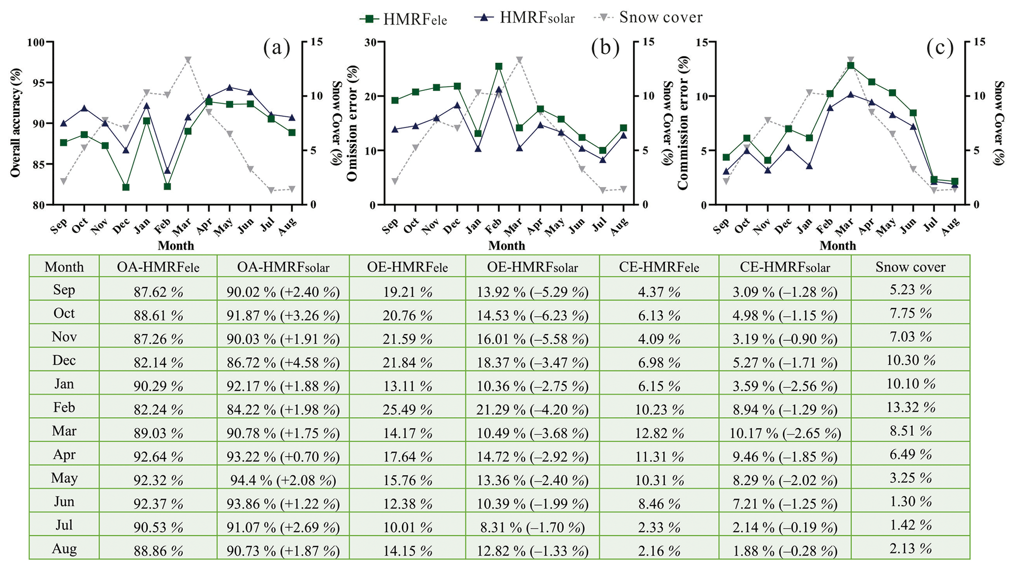
Figure 4 Temporal variations in OA (overall accuracy) (a), OE (omission error) (b), and CE (commission error) (c) of HMRF_ele- and HMRF_solar-based snow products from 2002–2021.

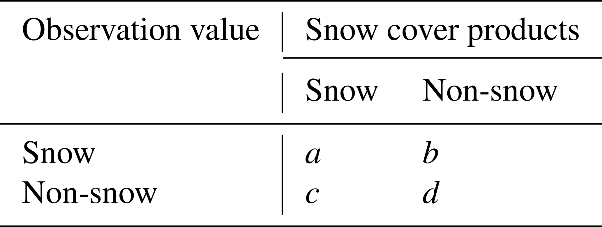
Table 1 Confusion matrix comparing snow cover products with observation value.

The three validation indices are defined as follows:

$$\begin{array}{}\text{(17)}& {\displaystyle }\mathrm{OA}=\left({\displaystyle \frac{a+d}{a+b+c+d}}\right)\times \mathrm{100}\mathit{\%}\text{(18)}& {\displaystyle }\mathrm{OE}=\left({\displaystyle \frac{b}{a+b}}\right)\times \mathrm{100}\mathrm{\%}\text{(19)}& {\displaystyle }\mathrm{CE}=\left({\displaystyle \frac{c}{c+d}}\right)\times \mathrm{100}\mathrm{\%}.\end{array}$$

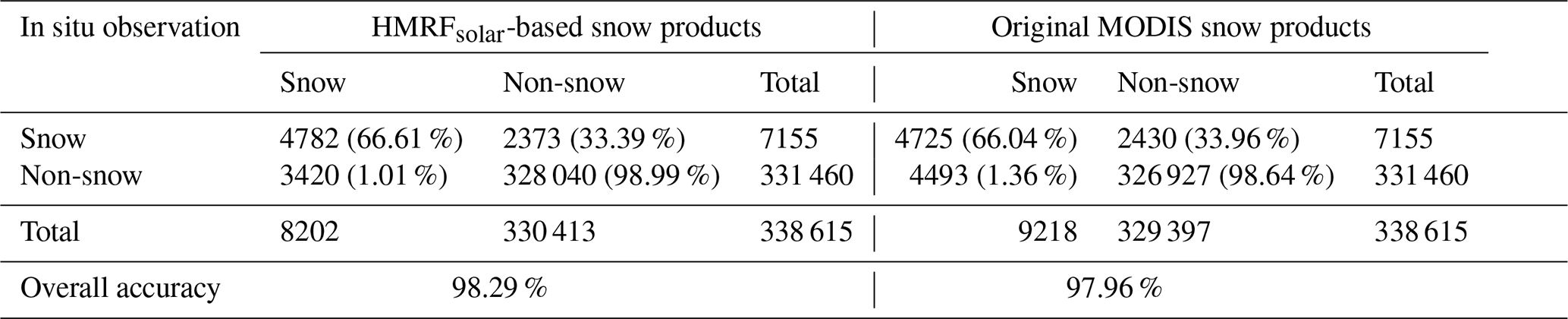
Overall accuracy (OA) is the probability a pixel that is correctly classified; and omission error (OE) and commission error (CE) represent the underestimated and overestimated snow pixels, respectively. We first compared our daily HMRF_solar-based and original MODIS snow products with snow depth observed from 137 in situ stations from 2002–2021 (Table 2). The OA of all gap-free pixels in original MODIS products was 97.96 %. After employing the HMRF_solar-based method, the OA of these gap-free pixels was increased to 98.29 %. The OE was reduced by 0.57 %. Since the in situ stations in the TP are primarily distributed in low-altitude areas (Fig. 1a), only using in situ observations may not be representative and lead to biases in the accuracy assessment. Therefore, we also conducted evaluation in comparison with snow cover mapped from Landsat data obtained from 2002–2021, and regarded it as the true verification value in the following accuracy evaluation.

Table 2 Confusion matrices between HMRF_solar-based, original MODIS snow products and in situ observation for gap-free pixels in original MODIS snow products during 2002–2021.

4.2 Accuracy assessment based on Landsat data

A total of 81 Landsat-8 images (Fig. 1a, Table A1) with less than 2 % cloud coverage were selected for this accuracy assessment. We constructed the confusion matrices for the HMRF_solar-based snow cover products, HMRF_ele-based snow products, and original MODIS snow cover products against snow cover mapped from Landsat series data products (Table 3). The OA for gap-free pixels in original MODIS products was 89.31 %. When we used surface elevation to represent the environmental association in HMRF modeling technique, the OA of these gap-free pixels was increased to 90.47 %. Since using surface elevation only cannot well-represent the influence of complex topography on snow cover distribution over the TP, this improvement is still limited. After incorporating the solar radiation to model the comprehensive influence of multiple topographic factors on snow cover, the OA of our HMRF_solar-based snow products was increased by 2.06 % compared with the OA of original MODIS products. C. Liu et al. (2020) indicated that the classification errors in original MODIS snow products were strongly affected by OE. Our snow cover product provided a considerable improvement in this respect. The OE of our HMRF_solar-based snow products was 3.24 % lower than that of original MODIS products (Table 3).

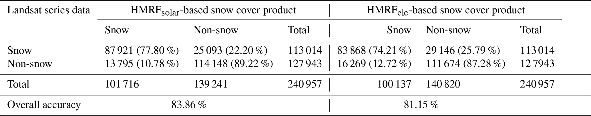
Particularly, our HMRF method is able to fill data gaps in original MODIS products in which spectral information is unavailable caused by cloud, by integrating spatiotemporal and environmental information together. Table 4 shows that the OA of the HMRF_solar- and HMRF_ele-based snow cover products for those data-gap pixels in original MODIS products was 83.86 % and 81.15 %, which is 7.50 % and 9.32 % lower than that of gap-free pixels. It is also showed that the OA of HMRF_solar-based snow cover product is 2.71 % higher than that of HMRF_ele-based snow cover product. Both Tables 3 and 4 confirmed that using solar radiation as the environmental information in the HMRF framework can develop more reliable snow cover products.

Figure 5 Effect of elevation on OA (a), OE (b), and CE (c) of HMRF_ele- and HMRF_solar-based snow products from 2002–2021.

4.3 Accuracy improvement in different times of a snow season

To explore the details of snow cover variation, we define the snow season from September of the previous year to August of the following year, for example, the time range of the 2002 snow season is 1 September 2002–31 August 2003​​​​​​​ (Chen et al., 2018b). Previous studies (Huang et al., 2018; Klein, 2003; X. Li et al., 2019) have suggested that the snow cover estimation accuracy was generally low during snow transitional period (i.e., the beginning and end of a snow season). We plotted the temporal variations in the OA, OE, and CE of the HMRF_solar- and HMRF_ele-based snow cover products (Fig. 4). Except November, December, and February, the OAs of the new snow products were more than 90 % in all months. The accuracy was relatively low during snow transitional period (November, December, and February to April), whereas the accuracy was higher in snow stable period. The trend of the CE was almost the same as that of snow cover; that is, the months with more snow cover had a larger CE. However, the CE was generally low in all months. By comparison with the HMRF_ele-based products, the accuracy of our new products was higher in almost all months. In addition to the stable snow period, the improvement for transition period was also notable, which increased by an average of 2.18 %. In transition period, with rapid temperature changes, the snow status changed rapidly, and the snow mapped by MOD10A1 (crossing at 10:30) and MYD10A1 (crossing at 13:30) were different because of the different temperatures and solar radiation. The original MODIS snow cover products have relatively high error during snow transitional period (Y. Li et al., 2019​​​​​​​). After incorporating solar radiation as an environmental contextual information in HMRF, the accuracy of snow cover products has been improved effectively.

Table 3 Confusion matrices between HMRF_solar-based snow products, HMRF_ele-based snow products, original MODIS snow products, and snow cover mapped from Landsat series data products for gap-free pixels during 2002–2021.

Table 4 Confusion matrices between HMRF_solar-based snow cover products, HMRF_ele-based snow cover products, and snow cover mapped from Landsat series data products for data-gap pixels during 2002–2021.

4.4 Accuracy improvement for different surface topography

We divided the elevation of the study area into four categories: <3000, 3000–4000, 4001–5000, and >5000 m, to explore the effect of elevation on snow cover. We then calculated the snow cover products accuracy in each category. Figure 5 indicates that the OA of the products decreased with increasing elevation. The accuracy of our products was highest in the <3000 m category (94.26 %). With increasing elevation, the OE first decreased and then increased; that is, the OE value was the lowest in the 4001–5000 m category, whereas the CE was the highest in the 4001–5000 m category. Li et al. (2020) established the effect of elevation on snow cover and also demonstrated the accuracy of original MODIS snow products generally decreased with increasing elevation. Areas at higher elevation generally receive more solar radiation; hence, the snow status changes more rapidly at higher elevations, resulting in decreased snow cover estimation accuracy.

By comparison with the HMRF_ele-based products, the accuracy of our new products was higher in almost all elevation categories, and as the elevation increased, the accuracy improvement was more remarkable (reaching an improvement of 3.16 % in the >5000 m category). The improvements in OE first decreased and then increased; that is, the accuracy improvement of the OE value was the smallest in the 4001–5000 m category, with an improvement of 3.47 %. The CE exhibited the opposite trend; that is, the accuracy improvement in the CE value was the largest in the 4001–5000 m category, at 2.33 %. The accuracy improvement provided by our new snow cover product was substantially increased with the increase in elevation, indicating its effectiveness in high-altitude areas.

To explore the effect of slope on snow cover, we divided the slope of the study area into five categories: <10, 10–20, 21–30, 31–40, and >40^∘. The OA of the snow cover products decreased with increasing slope, which is consistent with the trend of the changes in accuracy with increasing elevation (Fig. 6). The accuracy of our new products was highest in the 0–10^∘ category, with a value of 93.78 %. The OE was high for relatively low-slope areas (<30^∘), and the CE was high for high-slope areas (≥30^∘).

By comparison with the HMRF_ele-based products, the accuracy of our new products was higher in almost all slope categories, and the accuracy improvement was remarkable in the 10–20^∘ category (reaching an improvement of 2.90 %). This means topography of 10–20^∘ slopes had the strongest impact on snow cover on the TP. The accuracy improvements in OE decreased with increasing slope, whereas the accuracy improvements in CE increased with increasing slope. In the <10^∘ category, the improvement in CE was the smallest, at 0.56 %, whereas the improvement in OE was the largest, at 6.83 %. In the >40^∘ category, the improvement in CE was the largest, at 2.20 %, whereas the improvement in OE was the smallest, at 0.81 %.

Figure 6 Effect of slope on OA (a), OE (b), and CE (c) of HMRF_ele- and HMRF_solar-based snow products from 2002–2021.

Finally, we explored the effect of aspect on snow cover (Fig. 7). The OA of the snow cover products was higher on shaded slopes than on sunny slopes. The OAs of our new products on sunny and shaded slopes were 88.37 % and 90.07 %, respectively. By comparison with the HMRF_ele-based products, the accuracy improvement provided by our new products was remarkable on sunny slopes (improvement of 3.16 %) than on shaded slopes (improvement of 1.75 %), corresponding with the actual situation. The improvement in the OE on sunny slopes was also remarkable (improvement of 3.63 %).

Figure 7 Effect of aspect on OA (a), OE (b), and CE (c) of HMRF_ele- and HMRF_solar-based snow products from 2002–2021.

5 Discussion

5.1 Effect of the HMRF_solar-based snow cover products over complex terrain

Long-term and high-precision snow cover products are key to the snow hydrology research in the TP. Compared to the heterogeneous land cover, complex terrain has more severe effects on MODIS snow products in the TP (C. Liu et al., 2020; Azizi and Akhtar, 2021). To enhance snow detection accuracy in mountainous areas, we used solar radiation as the environmental contextual information rather than surface elevation used in the original HMRF_ele modeling technique (Huang et al., 2018). The calculated optimal parameters used in Eq. (1) could reflect the importance of each energy to a certain extent. The optimal parameters of the HMRF_solar-based products for spectral, spatial–temporal, and environmental information were 0.117, 1.294, and 0.532, respectively, while that of the original HMRF_ele-based products were 0.338, 1.419, and 0.576, respectively. The proportion of environmental information of HMRF_solar-based products (27.37 %) were higher than that of HMRF_ele-based products (24.70 %), which shows the improvement of HMRF_solar-based products over complex terrain. Moreover, Fig. 8a shows a true-color Sentinel-2B image. Figure 8b, c, and d show the original MODIS, HMRF_ele- and HMRF_solar-based snow cover products, respectively, on 31 October 2018. The examples in Fig. 8 (where the topography has a dominant effect on snow cover) show that the original HMRF_ele-based snow cover products mapped all data gaps in the shaded and sunny slopes at the same elevation as snow-covered pixels; however, after incorporating solar radiation, our new products accurately identified them as non-snow-covered pixels. In general, since sunny slopes receive relatively more solar radiation, the area of snow cover on sunny slopes is smaller than that on shaded slopes. The new HMRF_solar-based snow products more effectively filled the data gaps on sunny slopes, producing more realistic results. Solar radiation was particularly effective as an environmental contextual factor to correct the snow detection errors in mountainous areas.

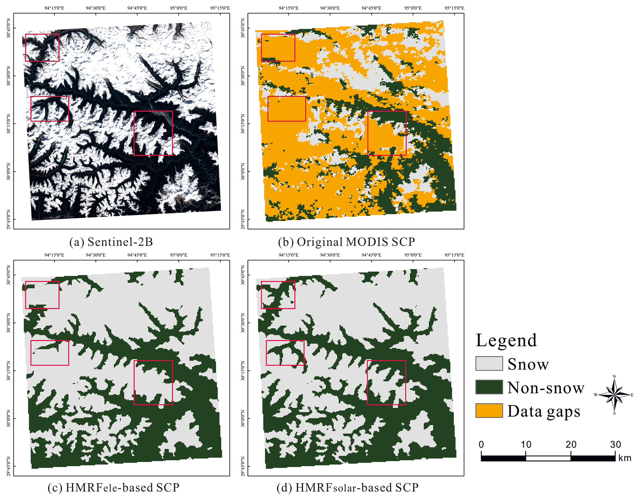
Figure 8 Comparison between true-color Sentinel-2B imagery (a), original MODIS snow products (b), HMRF_ele-based snow products (c), and HMRF_solar-based snow products.

5.2 Potential applications of the HMRF_solar-based snow cover products

Compared with in situ observations, the overall accuracy of snow cover products on the TP reported by other studies is in the range of 90.74 %–96.6 %, and the OE is greater than the CE (Yu et al., 2016; Xu et al., 2017; Zheng and Cao, 2019). The overall accuracy of our new snow products is 98.29 % in comparison with in situ observations, and the new product has a considerable improvement in OE. The new snow cover products provide spatiotemporally continuous snow cover distribution at 500 m resolution over the past two decades, thus having a great application potential for analyzing the processes of snow accumulation and melting. Figure 9 shows the snow cover trends over a sample area (location shown in Fig. 1) from our daily gap-free snow products and 8 d composite MODIS snow products on Terra (MOD10A2 v6.1) (Hall and Riggs, 2021​​​​​​​) during the 2017 snow season. We chose this sample region because it covers more mountainous areas including Hengduan Mountain and Bayankala Mountain, and has seasonal snow for multiple years. The MOD10A2 v6.1 products composite 8 d MODIS data to reduce the data gaps in the original daily MODIS snow products, and represent the maximum snow cover extent in 8 d, which means once snow is identified on any day in the 8 d time window, the pixel is mapped as snow. Although the overall variation trends of snow cover are similar between these two products, the snow cover percentage obtained from the MOD10A2 v6.1 data was 19.60 % higher than that of daily products during the 2017 snow season. The status of the snow in the TP changes rapidly. Compared with the 8 d composite MODIS snow products (MOD10A2 v6.1), the HMRF_solar-based snow cover products can get more detailed and accurate information on snow accumulation and melting processes, particularly during the snow transitional periods (February to April and November to December) when short-term snowfall events occur frequently (Fig. 9). In addition, owing to its high temporal resolution (daily) and long-term spatiotemporal continuity, the generated snow cover products also provide important baseline information for monitoring climate change, calibrating hydrological models, and simulating snowmelt runoff in the TP.

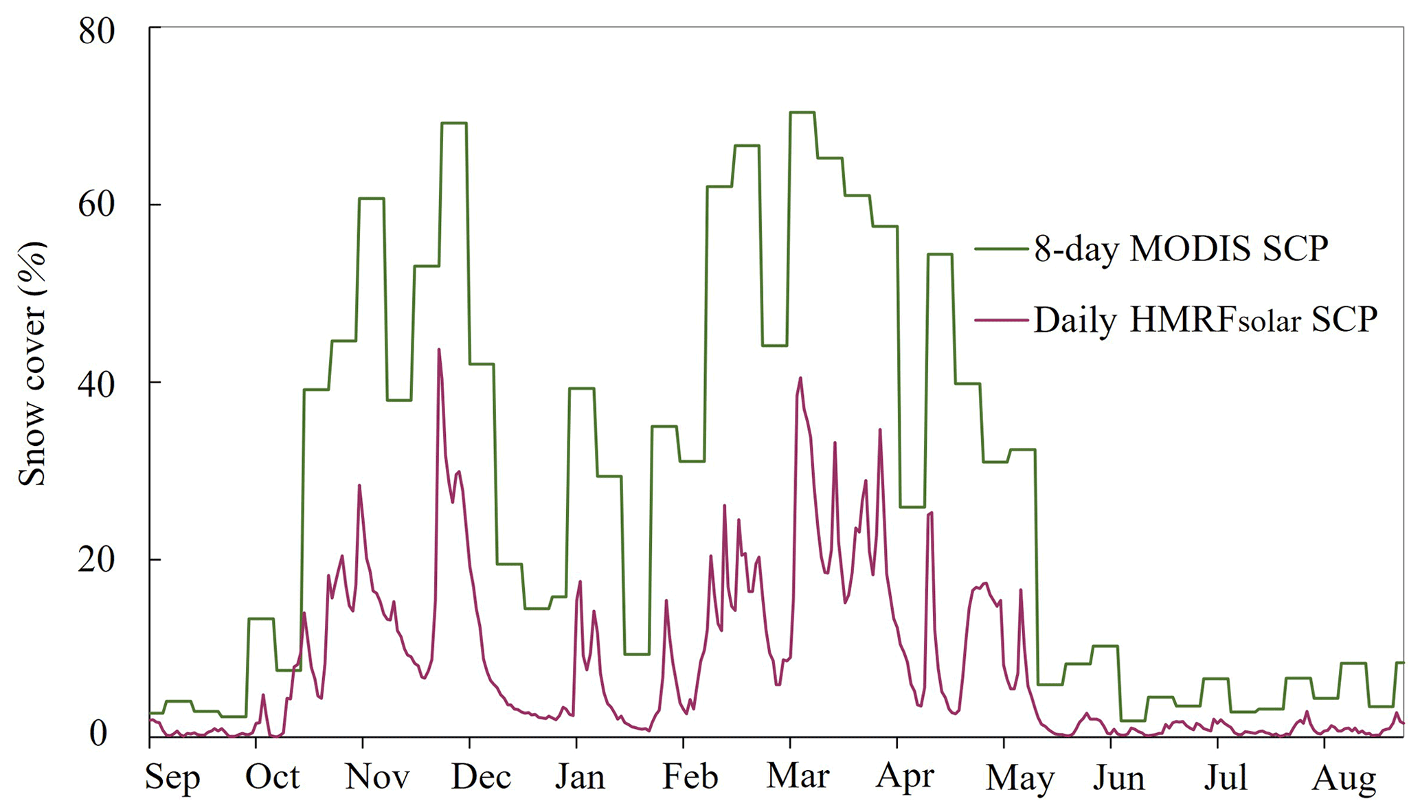
Figure 9 Snow cover percentage for daily HMRF_solar-based snow cover products and 8 d composite MODIS snow products in a sample area during the 2017 snow season of the TP. (SCP stands for snow cover products.)

5.3 Limitations of the HMRF_solar-based snow cover products

The accuracy evaluation for the new snow cover products had some limitations. The majority of in situ observations in the TP are distributed in the low-altitude areas in the east, with only 22 % located in high-altitude areas (Fig. 1a). The number of in situ observations in the snow category was considerably smaller than that in the non-snow category, which created challenges in verifying snow category classification (Zhang et al., 2021). C. Liu et al. (2020) demonstrated that compared to in situ observations, snow cover mapped from Landsat series images is more related to MODIS snow cover products owing to the closer spatial match. Therefore, the conclusions about the new snow products were based on the accuracy evaluation against Landsat images, which may still contain some bias. Additionally, the solar radiation indicated used only imitates the solar radiation under clear-sky conditions. In a follow-up study, we will simulate the solar radiation throughout the year according to the weather conditions (e.g., the effect of cloud cover), and use parallel calculations to enhance calculation efficiency and further improve the snow cover product accuracy.

6 Data availability

The long-term daily snow cover products produced here are gap-free at 500 m resolution under the Universal Transverse Mercator (UTM zone 45) projection, and can be freely accessed from the National Tibetan Plateau Data Center at https://doi.org/10.11888/Cryos.tpdc.272204 (Huang and Xu, 2022), which is stored as a zip file (∼ 1.61 GB) for each year. By uncompressing the zip file, the daily snow cover data are provided in GeoTIFF format, and the values in the snow cover products are classified as snow (1) and non-snow (2). The name of each file is “HMRFSTP_yyyyddd.tif”, in which HMRFSTP is the abbreviation of “hidden Markov random field-based snow cover products for Tibetan Plateau”, yyyy stands for year, and DDD stands for Julian day, such as 2002135.tif describes the snow cover on Tibet Plateau on the 135th day of 2002.

7 Conclusions

In this study, we generated long-term daily gap-free snow cover products at 500 m resolution from original MODIS snow products in the TP over the past two decades. The snow cover estimate accuracy was greatly improved by incorporating solar radiation as a surrogate for environmental contextual information in HMRF framework in mountainous areas. We validated and evaluated our snow cover products through comparison with in situ observations and high-resolution snow cover mapped from Landsat images, with accuracy estimates of 98.29 % and 91.36 %, respectively. Our evaluation also suggests that incorporating solar radiation, instead of the simple use of surface elevation as the environmental contextual information in HMRF framework, results in the accuracy of the snow products increases by 2.71 % and the OE decreases by 3.59 %. Specifically, the accuracy of the new snow products is particularly improved during snow transitional period and over complex terrains with high elevation and sunny slopes.

We believe that the long-term and spatiotemporally continuous snow cover products generated in this study have great potential to analyze the processes of snow accumulation and melting, to monitor climate change, and to understand hydrological cycling in the TP.

Appendix A

Table A1 Landsat series images used for assessment of the HMRF-based snow cover products in this study.