The NIEER AVHRR snow cover extent product over China – a long-term daily snow record for regional climate research

A long-term Advanced Very High Resolution Radiometer (AVHRR) snow cover extent (SCE) product from 1981 until 2019 over China has been generated by the snow research team in the Northwest Institute of Eco-Environment and Resources (NIEER), Chinese Academy of Sciences. The NIEER AVHRR SCE product has a spatial resolution of 5 km and a daily temporal resolution, and it is a completely gap-free product, which is produced through a series of processes such as the quality control, cloud detection, snow discrimination, and gap-filling (GF). A comprehensive validation with reference to ground snow-depth measurements during snow seasons in China revealed the overall accuracy is 87.4 %, the producer's accuracy was 81.0 %, the user's accuracy was 81.3 %, and the Cohen's kappa (CK) value was 0.717. Another validation with reference to higher-resolution snow maps derived from Landsat-5 Thematic Mapper (TM) images demonstrates an overall accuracy of 87.3 %, a producer's accuracy of 86.7 %, a user's accuracy of 95.7 %, and a Cohen's kappa value of 0.695. These accuracies were significantly higher than those of currently existing AVHRR products. For example, compared with the well-known JASMES AVHRR product, the overall accuracy increased approximately 15 %, the omission error dropped from 60.8 % to 19.7 %, the commission error dropped from 31.9 % to 21.3 %, and the CK value increased by more than 114 %. The new AVHRR product is already available at https://doi.org/10.11888/Snow.tpdc.271381 (Hao et al., 2021).

1 Introduction

Snow cover is closely bound up with our climate. On the one hand, owing to snow's unique optical properties (high albedo) it can affect the surface radiation budget severely and thereby our climate systems significantly (Warren, 1982; Huang et al., 2019). On the other hand, changes in climate in turn affect global and regional snow covers. With the continuous warming of the global climate, snow cover on the Earth has been clearly shrinking over the past several decades (Barnett et al., 2005; Bormann et al., 2018). Therefore, long-term snow cover data are not only particularly important for climate research but also an indispensable indicator of climate change.

Remote sensing is a widely used tool for monitoring snow cover extent (SCE) globally and regionally at various spatial and temporal resolutions (Konig et al., 2001; Dozier and Painter, 2004; Frei et al., 2012; Wang et al., 2014) since the beginning of the satellite era in the 1960s. The Northern Hemisphere Weekly Snow Cover and Sea Ice Extent (NHSCE) product provides weekly SCE with spatial resolutions of about 190 km from 1966 to 1997 (Robinson et al., 1993). Although the time coverage is long, the NHSCE product has a low spatiotemporal resolution, hand-drawn snow line maps, and incomplete spatial coverage due to swath gaps or cloud obscuration, largely restricting its application in climate research. With the development of satellite sensors, SCE products with high spatial resolution have been issued in the last decades, such as the Interactive Multisensor Snow and Ice Mapping System (IMS), which provides daily SCE with spatial resolutions of 24, 4, and 1 km from 1997 to the present (Helfrich et al., 2007; Ramsay, 1998). The Moderate Resolution Imaging Spectroradiometer (MODIS) provides daily SCE with a spatial resolution of 500 m from 2000 to the present (Hall et al., 2002; Riggs et al., 2017). The Fengyun daily SCE products have a spatial resolution of 1 km from 2003 to the present (Min et al., 2021). These SCE datasets have good quality with a high spatiotemporal resolution, but their short period is insufficient to create a climatological baseline of snow cover.

The Japan Aerospace Exploration Agency (JAXA) recently issued the long-term SCE product JASMES with a spatial resolution of 5 km throughout the Northern Hemisphere. This product consists of satellite-derived daily, weekly, and half-monthly averaged global snow covers derived from 5 km resampled radiance data of Advanced Very High Resolution Radiometer (AVHRR) Global Area Coverage (GAC) radiance data on board NOAA series satellites (1978–2001) and MODIS on board the Terra and Aqua satellites (2000–the present) (Hori et al., 2017). Although the JASMES product presented a long time series and significantly enhanced spatial and temporal resolutions, several shortcomings have been found. (1) The JASMES product uses AVHRR before 2000 and MODIS data after 2000. Although calibrated by the authors, the bandwidths of the two sensors are not consistent, and using the same algorithms for both can cause discontinuities in the data. (2) Previous work showed that the JASMES snow product has an excessive cloud mask which would cause a considerable number of snow pixels to be misidentification as cloud pixels (Wang et al., 2018). (3) JASMES snow algorithm tended to underestimate snow in China, especially on the Qinghai–Tibet Plateau (Wang et al., 2018). (4) Finally, JASMES SCE exhibits incomplete spatial coverage caused by clouds and data gaps. These shortcomings limit its application in snow monitoring and climate studies in China. Thus, China still lacks a high-quality, long-term SCE product with complete spatial coverage for climate research.

Therefore, a new daily 5 km gap-free AVHRR snow cover extent product for China was produced based on the Google Earth Engine platform from 1981 to 2019. The new product provides a long time series of SCE with high quality for China and makes six improvements. (1) The Climate Data Record (CDR) of AVHRR surface reflectance (SR) is used as a data source after 2000 rather than MODIS to ensure product continuity. (2) Considering sensor attenuation of Band 11 before and after 2000, the algorithm chooses different training samples and discriminant thresholds separately. (3) An improved cloud detection test and new thresholds are obtained by a volume of training data which can solve the snow/cloud confusion. (4) A multi-level decision tree for the snow discrimination algorithm is applied which significantly improved snow discrimination accuracy. (5) Improved gap-filling (GF) strategies are adopted to obtain complete snow coverage. (6) Land surface temperature (LST) reanalysis is used to exclude the false snow identification. Due to these improvements, the new AVHRR SCE product may serve as a baseline record for climate and other related applications.

2 Datasets and preprocessing

2.1 AVHRR surface reflectance CDR

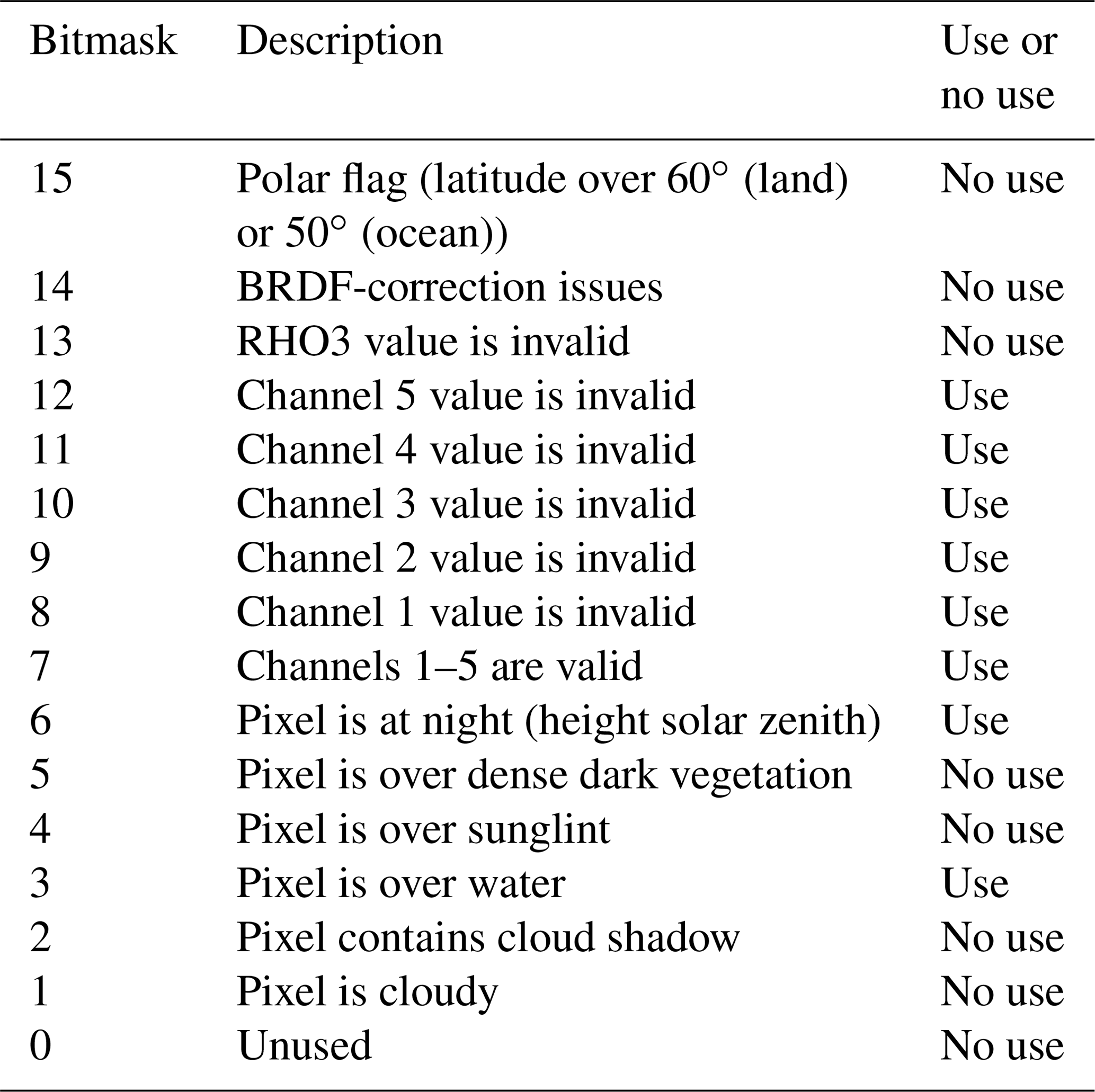
The NOAA CDR of AVHRR Surface Reflectance Version 4 (AVHRR SR V4) was used as basic input data. AVHRR SR V4 is generated using AVHRR GAC Level 1B data through geolocation, calibration, and atmospheric correction, and it has latitudinal and longitudinal dimensions of 3600×7200, covering the globe at 0.05^∘ spatial resolution (Vermote et al., 2014). The dataset contains surface reflectance, brightness, temperatures, and quality control flags for the period between 24 June 1981 and 16 May 2019. Google established the Google Earth Engine (GEE) cloud computing platform in 2012. GEE enables academics to quickly access massive amounts of remote sensing data without downloading it, which could support scientific analysis and visualization of geospatial datasets at petabyte scale (Gorelick, 2012). In this study, all AVHRR SR V4 images were processed by GEE cloud platform. The reflectance, brightness, and temperature data are described in Table 1. The quality control flags are summarized in Table 3.

Table 1 The details of spectral bands from the CDR of AVHRR Surface Reflectance Version 4 from GEE platform.

2.2 Landsat-5 TM snow map

This study used two groups of Landsat-5 Thematic Mapper (TM) maps across China from 1985 to 2013. The first group was used as “true” values to acquire the training data of AVHRR surface reflectance. TM snow maps were produced by the improved “SNOMAP” algorithm developed by Chen et al. (2020) for the snow season (beginning on 1 November through 31 March of the following year). Each map contained three classes, namely snow, non-snow, and cloud. Considering sensor attenuation before and after 2000, the algorithm chose different TM images separately. Table 2 shows the number of Landsat-5 TM scenes used for training before and after 2000. The second group of maps was used as ground truth values to evaluate the AVHRR SCE product. A total of nine Landsat-5 TM snow maps were used as the validation dataset (Fig. 1). To ensure reliability and representativeness, the training and validating samples were evenly distributed in three major seasonally snow-covered regions across China's mainland, including north Xinjiang, Northeast China, and the Qinghai–Tibet Plateau.

Table 2 The number of training scenes using Landsat-5 TM.

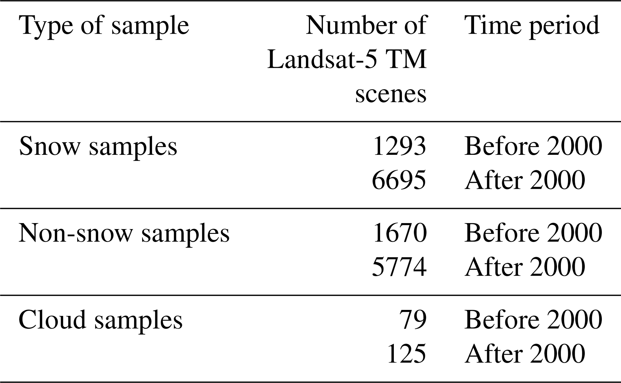
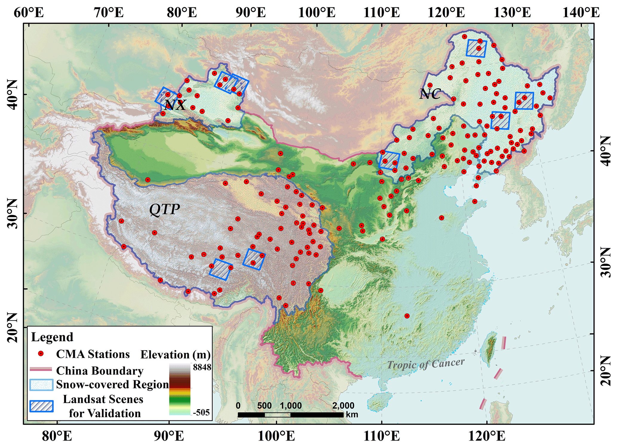
Figure 1 The geographic location of study area and the spatial distribution of major snow-covered regions, climate stations, and Landsat-5 validation dataset. The elevation data were derived from Shuttle Radar Topography Mission (SRTM).

2.3 AVHRR training samples

Snow and non-snow training samples from the AVHRR were generated from spatially and temporally (same day) collocated AVHRR surface reflectance along with the Landsat-5 snow maps. Cloud training samples came from AVHRR surface reflectance with Landsat-5 cloud flags during summer (1 June to 31 August). The training samples before 2000 included 717 172 snow samples, 804 104 non-snow samples, and 82 904 cloud samples. Samples after 2000 included 7 304 310 snow samples, 8 394 959 non-snow samples, and 44 422 cloud samples.

2.4 Ground snow-depth measurements

Ground snow-depth measurements provided by the China Meteorological Administration (CMA) were used to validate the AVHRR SCE products. Daily snow depth was measured near the stations using a professional meter ruler. All measurements were conducted at 08:00 Beijing time when the fractional snow cover in the field of view was more than 50 % (C.M.A, 2003). Validation CMA stations were carefully selected because too many non-snow samples can affect the accuracy of the assessment. To ensure the validation reliability, the selected CMA stations had ≥20 d with true snow (>1 cm) at the CMA site per snow season (Metsämäki, 2016). Finally, a total of 191 meteorological stations at 38-year periods (from 1981 to 2019; Fig. 1) were used to validate the AVHRR SCE products. The available CMA stations were evenly distributed across the three major seasonally snow-covered regions in China.

2.5 Ancillary data

Che et al. (2008) and Dai et al. (2015) generated snow-depth data by using an inter-sensor calibration of multiple satellites' passive-microwave observations, which provides daily 0.25^∘ snow-depth data for China from 1979 to 2020, and this dataset of long-term daily snow depth in China is available at https://doi.org/10.11888/Geogra.tpdc.270194. This dataset was used as a supplement to the gap-filling strategies. We used the land surface temperature (LST) daily product to alleviate the cloud–snow confusion by averaging the hourly ERA 5 land climate reanalysis dataset on the GEE platform (Muñoz Sabater, 2019). Digital elevation model (DEM) data were used as auxiliary data in the cloud and snow discrimination algorithm, mask, and validation. The Shuttle Radar Topography Mission (SRTM) DEM product has an original resolution of 90 m and is also available on the GEE platform. To match with AVHRR products, these products were resampled or aggregated into 5 km.

3 Methodology

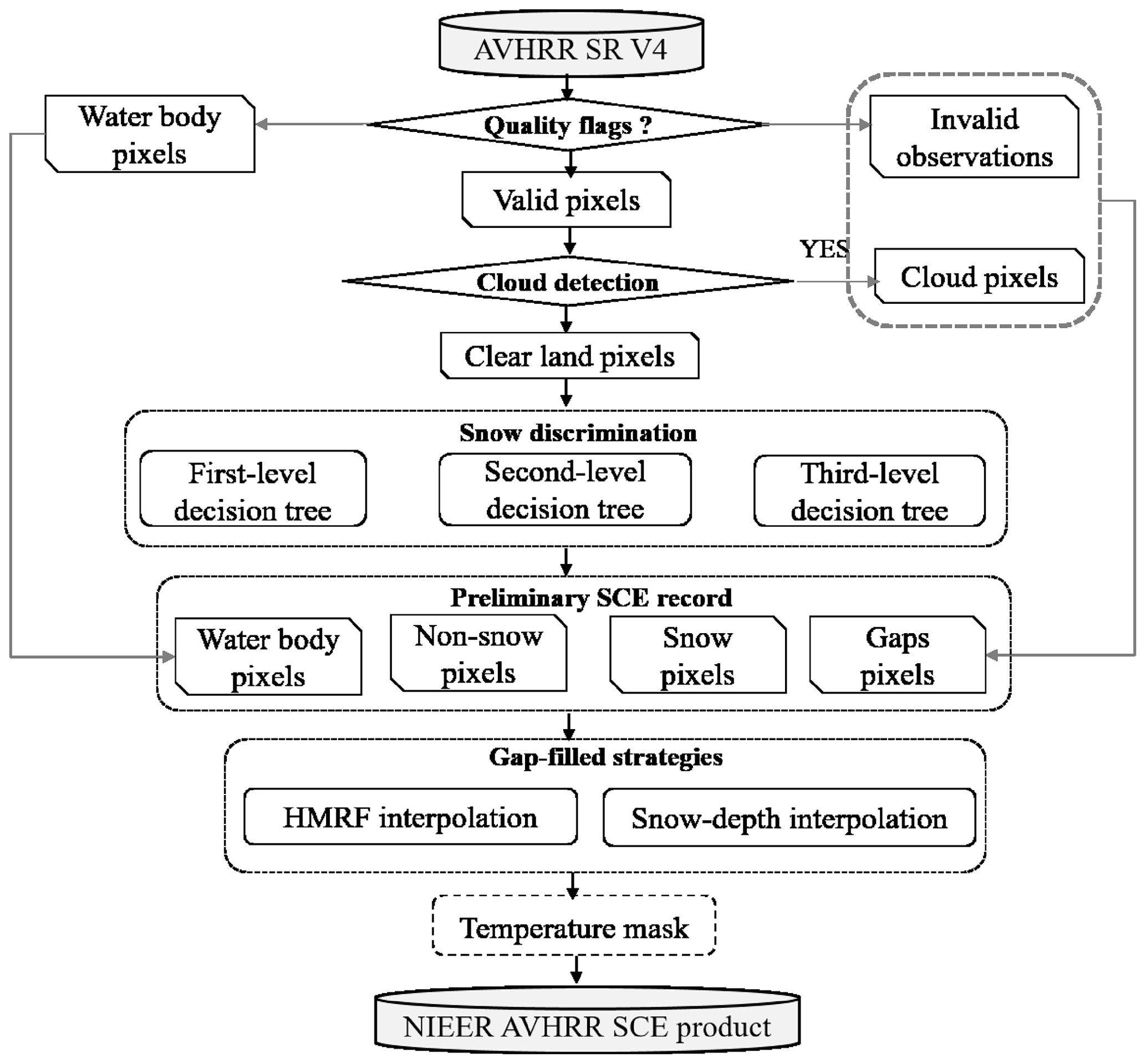
Figure 2 shows the different steps in the generation of the Northwest Institute of Eco-Environment and Resources (NIEER) AVHRR SCE product. Starting with AVHRR Surface Reflectance Version 4 (AVHRR SR V4) data on the GEE platform, valid observations were selected first by the quality control flags of AVHRR SR V4. Then, an improved cloud detection algorithm was developed to distinguish cloudy pixels, water pixels, and clear pixels. Third, clear pixels were determined as snow-covered or not by a multi-level decision tree, generating a set of AVHRR preliminary SCE records. Fourth, the gaps caused by clouds or invalid observations in the preliminary SCE record were filled with a set of gap-filling techniques, including HMRF-based (hidden Markov random field) interpolation and snow-depth interpolation. Finally, postprocessing based on land surface temperature and DEM was conducted to exclude false snow identifications.

Figure 2 Generation flowchart of NIEER AVHRR snow cover extent product (NIEER AVHRR SCE).

3.1 Quality control of AVHRR

Only observations valid in all AVHRR channels were employed to directly generate SCE records by using the quality control bit flags of AVHRR SR V4. Table 3 shows all the quality control information from AVHRR SR V4 and the status of usage in this study. After quality control processing, the valid pixels were used as input for retrieval, and the invalid pixels were regarded as gap pixels.

Table 3 The descriptions of quality control of AVHRR SR V4.

3.2 Cloud detection algorithm

In this study, we could not directly adopt the cloudy flags of AVHRR SR V4 due to the obvious cloud overestimation (Chen et al., 2018).

As stated by previous studies (Hori et al., 2007; Hori et al., 2017; Stamnes et al., 2007; Yamanouchi et al., 1987), the following eight variables were used in the cloud detection test: SR1, SR2, SR3, BT11, the reflectance differences between SR1 and SR2 (SR1-SR2), the brightness temperature (BT) differences between BT37 and BT11 (BT37-BT11), the BT differences between BT11 and BT12 (BT11-BT12), and the normalized difference vegetation index (NDVI). The calculation of the NDVI is based on formula (Eq. 1).

$$\begin{array}{}\text{(1)}& \text{NDVI}={\displaystyle \frac{\text{SR}\mathrm{2}-\text{SR}\mathrm{1}}{\text{SR}\mathrm{1}+\text{SR}\mathrm{2}}}\end{array}$$

For cloud detection, “BT37-BT11” was used as the primary test. We adopted the cloud test scheme by Hori et al. (2017), but the critical threshold value of BT37-BT11 was adjusted. As earlier thresholds of BT37-BT11 used a stronger cloud discrimination algorithm and ignored the cloud/snow confusion problem, further optimization was needed to minimize misclassification and the omission of clouds. Therefore, we focused on optimizing the cloud algorithm thresholds. Using the Landsat-5 TM maps for the true values, we trained the frequency distribution characteristics of BT37-BT11 for cloud and snow samples from AVHRR SR. Table 4 shows the cloud discrimination schemes, with 10 cloud detection schemes and 4 non-cloud schemes. With A1 type as an example, Fig. 3 shows the optimal BT37-BT11 determination scheme. Figure 3a presents the BT37-BT11 frequency distribution of cloud and snow training samples from AVHRR before 2000, and Fig. 3b presents the variation in the overall accuracy at different BT37-BT11 thresholds. Optimum accuracy (84.76 %) occurred at the cross-point of snow and cloud frequency distributions, with a BT37-BT11 threshold of 14.5 K. This cross-point also represents a compromise for cloud omission (10.49 %) and commission (19.92 %) errors. Thus, the final threshold value was 14.5 K according to the optimal overall accuracy (OA), which means that a pixel is classified as a cloud when BT37-BT11 > 14.5 K. Following the same procedure, the optimal BT37-BT11 thresholds were obtained from AVHRR data before and after 2000, as listed in Table 4.

Table 4 Cloud detection tests and the corresponding thresholds. Target A indicates high and cold land (elevation > 300 m and BT11 < 260 K), which has four types: A1–A4. Target B indicates the remaining land, which includes 10 types: B1–B10. The cloud detection test was conducted from the top of the list to the bottom for each target. If the switch of the cloudy flag was “on”, the pixel was set to cloudy when the threshold tests met the conditions listed on the right-hand side. If the switch was “off”, the pixel identified as cloudy in the previous tests was reset to clear.

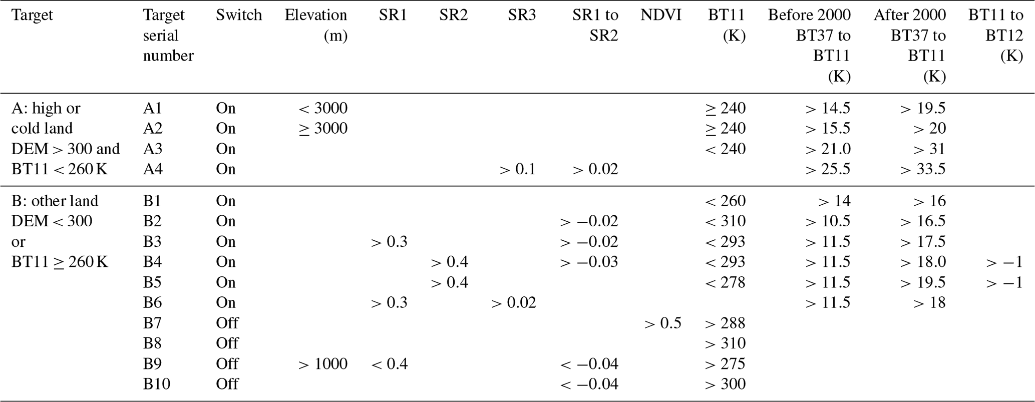
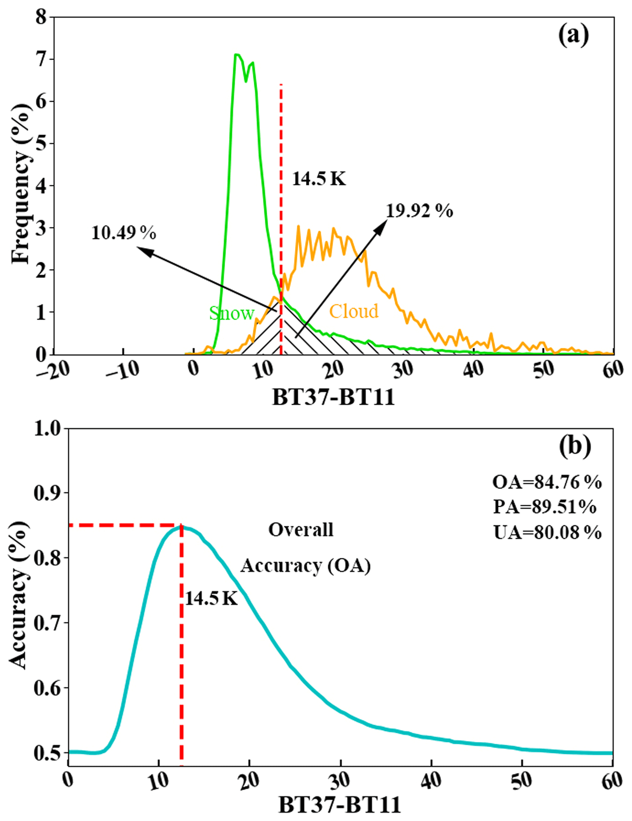
Figure 3 The frequency distribution of BT37-BT11 and optimal threshold acquisition of snow and cloud from A1 before 2000. Panel (a) shows the frequency distribution of snow and cloud on AVHRR, and panel (b) shows the determination of optimal threshold for cloud detection.

3.3 Snow discrimination algorithm

According to the previous snow classifications with AVHRR data (Hori et al., 2007; Hori et al., 2017; Stamnes et al., 2007; Yamanouchi et al., 1987), snow discrimination test variables included SR1, BT11, the reflectance ratio between SR3 and SR2 (SR3/SR2), reflectance differences between SR3 and SR2 (SR3-SR2), NDVI, the normalized difference snow index (NDSI), and BT differences between BT11 and BT12 (BT11-BT12). For snow discrimination, the NDSI was one of the primary tests. The NDSI is usually calculated using the green (around a wavelength of 0.50 µm) and shortwave infrared (around a wavelength of 1.60 µm) bands. As there were no shortwave infrared observations around 1.60 µm in AVHRR SR V4, we used the reflectance at 3.7 µm for an NDSI-like calculation, following Hori et al. (2017). The calculation of NDSI is shown in formula (Eq. 2).

$$\begin{array}{}\text{(2)}& \text{NDSI}={\displaystyle \frac{\text{SR}\mathrm{1}-\text{SR}\mathrm{3}}{\text{SR}\mathrm{1}+\text{SR}\mathrm{3}}}\end{array}$$

To improve the snow discrimination under clear-skies, all decision rules were re-adjusted according to the training samples from high-resolution snow maps. We developed a three-level decision tree algorithm which obtained the optimal threshold values from the training data. Using Landsat-5 TM data as true values, we obtained the frequency distribution characteristics of each band from AVHRR data in the snow and non-snow areas at SR1, BT11, SR3/SR2, SR3-SR2, NDVI, and NDSI. Figure 4 shows the flowchart of the three-level decision tree snow discrimination algorithm.

1. First-level decision tree. SR1, BT11 combined with DEM, and SR3/SR2 were chosen as first-level discriminators. The main purpose of the first-level decision tree is to exclude pixels that are definitely non-snow pixels. Snow has high reflectance in the SR1 band and low brightness temperature in the thermal infrared BT11 band. Since the ability to distinguish snow of SR3/SR2 is lower than SR3-SR2 by our training test, the SR3/SR2 was chosen as a first-level discriminator. Based on the frequency distributions of snow and non-snow pixels for the first-level discriminators for Landsat-5 TM maps, a confidence level of 95 % of snow samples was set to obtain the threshold value of certain non-snow pixels. As shown in Table 5, for the samples before 2000, SR1 >0.14 and BT11 < 274 K when DEM < 1300 m, BT11 <281 K when DEM ≥ 1300 m, and SR3/SR2 < 0.50 were the possible snow images, while the remaining pixels were non-snow pixels. The potential snow pixels were used as input for the second-level decision tree.

2. Second-level decision tree. NDVI and SR3-SR2 were chosen as second-level discriminators. The second-level decision tree was mainly used to obtain certain snow pixels from the possible snow pixels. Based on the frequency distributions of snow and non-snow pixels from potential snow pixels processed by the first-level decision tree, a confidence level of 99 % of non-snow samples was set to obtain the threshold value of certain snow pixels. For the samples before 2000, a pixel was classified as certain snow when $\text{NDVI}<-\mathrm{0.16}$ or SR3-SR$\mathrm{2}<-\mathrm{0.81}$ (Table 5). Other pixels were considered as the potential snow pixels, which were used as input for the third-level decision tree.

3. Third-level decision tree. NDSI was used as the third-level discriminator due to its excellent discrimination ability of snow cover and other land covers. Based on the frequency distributions of potential snow pixels derived from the second-level decision tree, the optimal NDSI threshold value was calculated by a method similar to that of the cloud test. Figure 5 shows the optimal NDSI scheme. Figure 5a presents the NDSI frequency distribution histogram of snow and non-snow pixels. The cross-point of snow and non-snow that has the highest overall accuracy (85.87 %) was chosen as the optimal NDSI threshold (0.73), as shown in Fig. 5b. The cross-point also represents a compromise for the snow omission (15.83 %) and commission error (13.03 %). Thus, pixels with NDSI > 0.73 were identified as snow for the samples before 2000.

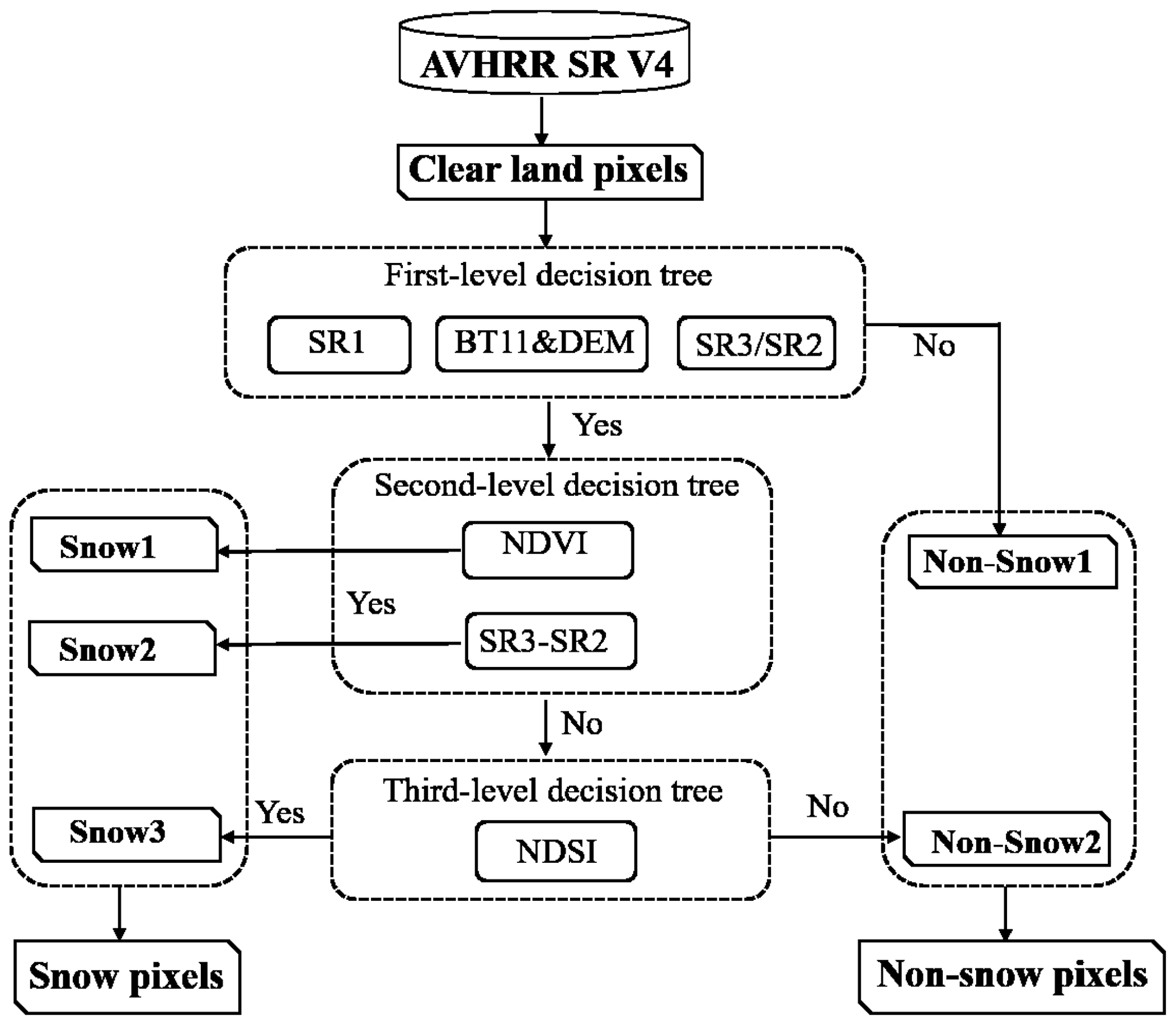
Figure 4 The flowchart of a three-level decision tree snow discrimination algorithm for NIEER AVHRR SCE product.

Table 5 Snow discrimination algorithm and its threshold values.

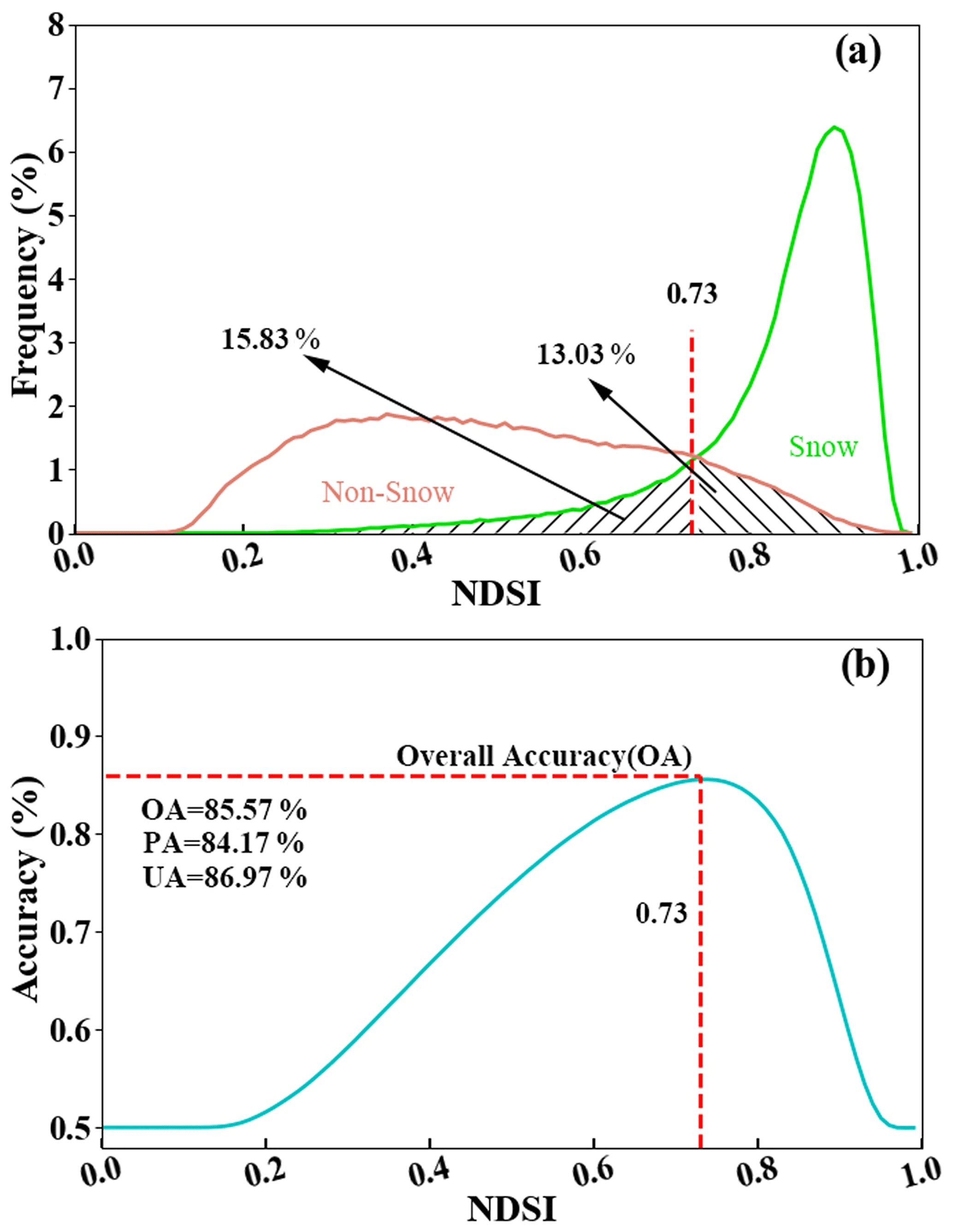
Figure 5 NDSI frequency distribution histogram and optimal threshold acquisition of snow and non-snow before 2000. Panel (a) is the frequency distribution of snow and non-snow on AVHRR, and panel (b) is the optimal NDSI threshold value.

Following the same strategy, optimal snow discrimination threshold values were obtained from AVHRR data before and after 2000 (Table 5). Using the above-mentioned algorithm, we produced the AVHRR preliminary SCE record for China based on the AVHRR SR V4.

3.4 Gap-filling strategies

For daily AVHRR preliminary SCE records, gaps caused by frequent cloud obscuration or swath gaps remained serious. Two gap-filling strategies described below were used to generate a spatially complete daily AVHRR SCE record.

3.4.1 HMRF-based spatiotemporal modeling

Here, we present a spatiotemporal modeling technique for filling up gap pixels in daily snow cover estimates based on the time series of AVHRR preliminary SCE records. The spatiotemporal modeling technique integrated AVHRR preliminary SCE spatial and temporal contextual information within an HMRF model (Melgani and Serpico, 2003). Initially, Huang et al. (2018) utilized HMRF-based spectral information, spatiotemporal information, and environmental information to reclassify snow and non-snow classes by MODIS snow products. In our study, we only used the spatiotemporal information for filling up gap pixels. The core of this method is computing the spatiotemporal cubic energy function for every gap from the neighborhood pixels and further classifying the gap pixels as snow pixels, non-snow pixels, or gap pixels using

$$\begin{array}{}\text{(3)}& U_{\mathrm{T}}\left({\mathit{\beta }}_n\right)=U_{\text{st}}\left({\mathit{\beta }}_n\left|N_{\text{sp}},N_{\text{tp}}\right.\right),\end{array}$$

where U_T is the total energy function of belonging to the class of β_n (n=2, β₁ denotes snow and β₂ denotes non-snow), and U_st is the spatiotemporal neighborhood cubic energy function. N_sp and N_tp denote the spatial neighborhood and temporal neighborhood centered with the gap pixel, respectively.

Figure 6 illustrates our gap-filling process based on the HMRF technique. For a given gap at the center, we first calculated U(β₁) and U(β₂) based on a spatiotemporal surrounding cube with $\mathrm{3}\text{rows}\times \mathrm{3}\text{columns}\times \mathrm{3}\mathrm{d}$. If U(β₁) >U(β₂), gap pixels were classified as snow pixels. Otherwise, they were classified as non-snow pixels. If U(β₁)=U(β₂) or there were not sufficient valid pixels for calculating U(β_n), we extended the spatiotemporal neighborhood to $\mathrm{3}\text{rows}\times \mathrm{3}\text{columns}\times \mathrm{5}\mathrm{d}$. If there were still insufficient valid pixels, the spatiotemporal neighborhood was expanded to $\mathrm{5}\text{rows}\times \mathrm{5}\text{columns}\times \mathrm{5}\mathrm{d}$. If the strategy above failed, gap pixels were maintained.

Figure 6 Diagram of the HMRF-based gap-filling process used in the study.

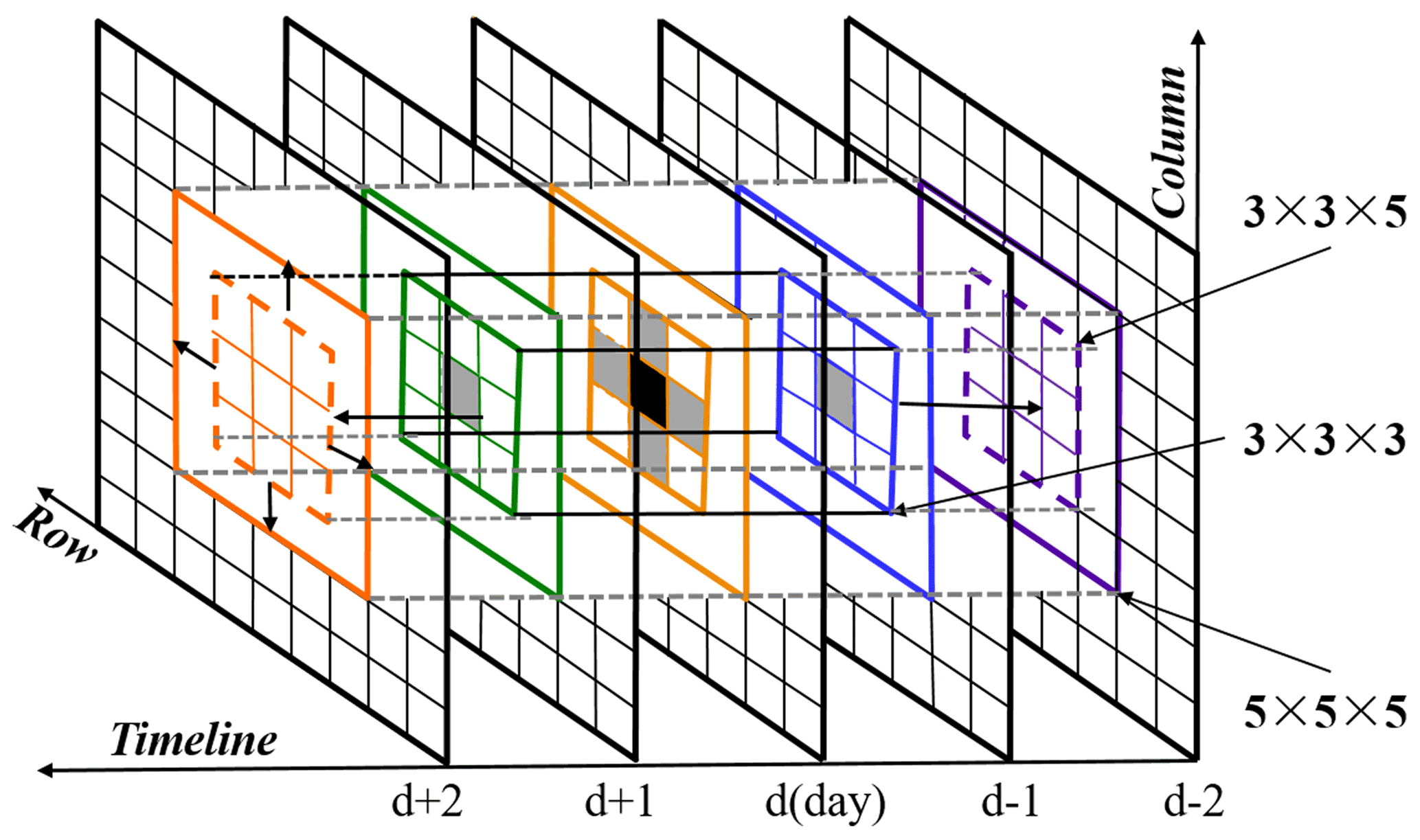
Table 6 The monthly average gap ratio of AVHRR preliminary SCE record in China before and after HMRF-based spatiotemporal interpolation from 1981 to 2019.

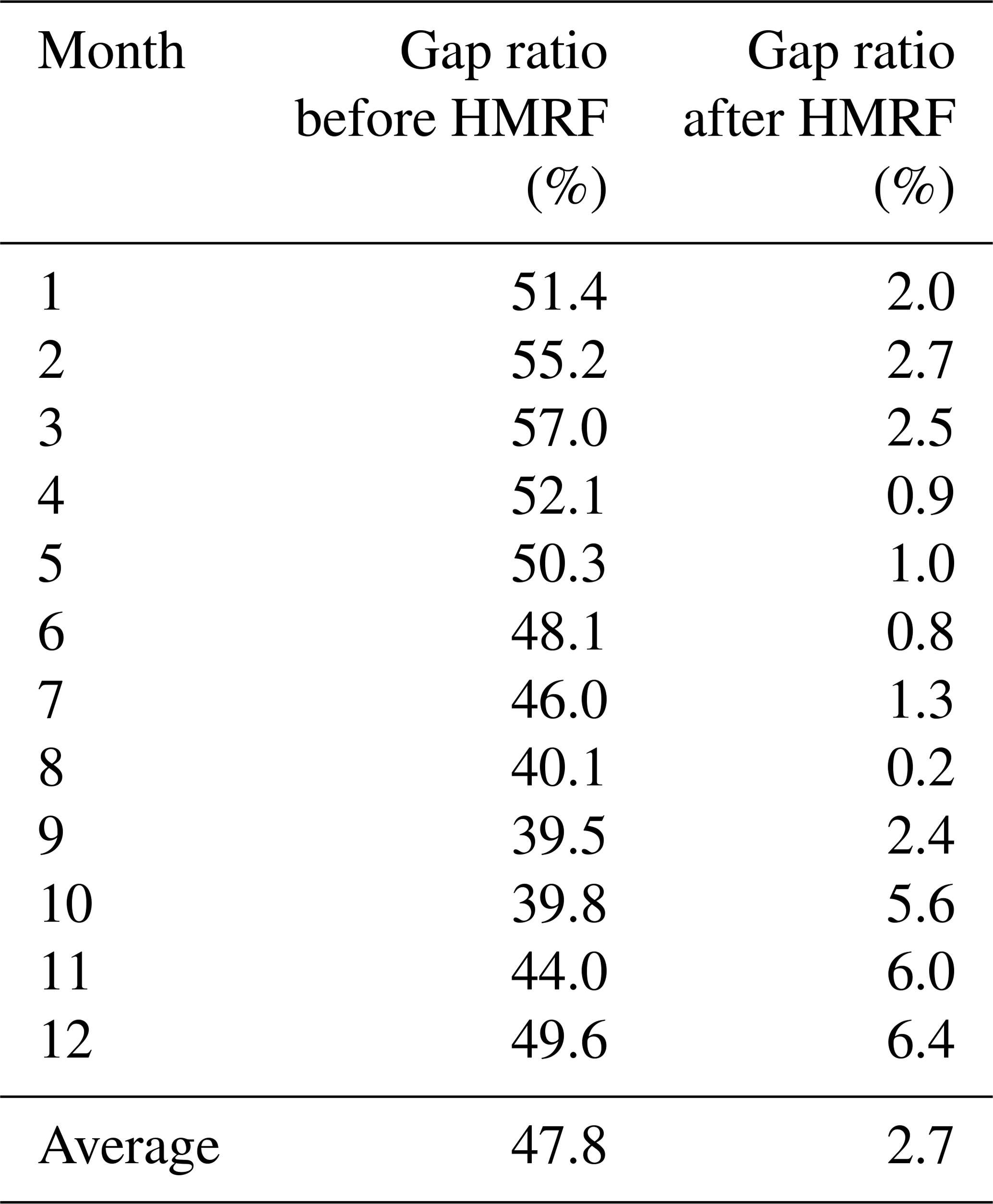
The HMRF-based modeling provided a rigorous interpolation framework for optimally integrating spatiotemporal contexts. To test the effect of HMRF-based interpolation for gap pixels, we compared the monthly average gap ratio of the AVHRR preliminary SCE record from 1981 to 2019 before and after HMRF-based interpolation (Table 6). The gap ratio of the AVHRR preliminary SCE record before HMRF-based interpolation was within 40 %–60 % (average: 47.8 %), and the gap ratio after HMRF-based interpolation ranged between 0.2 % and 6.4 % (average: 2.7 %). Almost 90 % of gap pixels could be reduced. The HMRF-based spatiotemporal model significantly improved the practicability of the AVHRR SCE product.

3.4.2 Interpolation based on passive microwave snow-depth data

Although most gap pixels were filled after interpolating the HMRF-based spatiotemporal model, there were still ∼6 % gaps left in the daily SCE data. Therefore, a fusion method combining the passive microwave daily snow-depth data and the AVHRR snow cover data was performed for these residual gap pixels. The passive microwave daily snow-depth data (25 km) were resampled to the same cell size as the AVHRR data (5 km) by the nearest neighbor interpolation method. If collocated snow depth was ≥2 cm, the gap was considered as a snow pixel. Otherwise, it was considered as a non-snow pixel (Hao et al., 2019).

3.5 Postprocessing based on surface temperature and DEM

Because of their similar optical properties, ice-cloud pixels are sometimes mistaken for snow pixels, which will result in artifact snow covers in southern China even during summers where and when snow is impossible. Referencing the MODIS algorithm, the postprocessing adopts LST products of ERA5 reanalysis and DEM to eliminate these snow pixels. The pixel is reclassified as snow-free under two condition: (1) LST ≥275 K and DEM ≤1300 km; (2) LST ≥281 K and DEM ≥1300 km.

4 Accuracies of the NIEER AVHRR SCE product

4.1 Metrics of accuracy evaluation

A confusion matrix similar to that given in Table 7 is used to assess all associated AVHRR SCE data in the paper. Four kinds of accuracy metrics were used in this study, following on previous studies (Dong et al., 2014; Zhang et al., 2019), including the OA, the producer's accuracy (PA), the user's accuracy (UA), and Cohen's kappa (CK) value. The OA is the fraction of the correctly detected cases and all cases. The PA measures the probability of correctly detected snow cases by AVHRR in the actual snow cases. The UA measures the proportion of true snow cases in all the detected snow cases by AVHRR. The sum of PA and omission error equals 1, and the sum of UA and commission error equals 1 (Arsenault et al., 2014). CK value is an overall measurement of the agreement and is considered a more robust metric than OA (Cohen, 1960; Powers and Ailab, 2011).

Table 7 Description of a confusion matrix of snow classification between NIEER AVHRR SCE product and truth value which reference ground snow-depth measurements or Landsat-5 TM SCE maps.

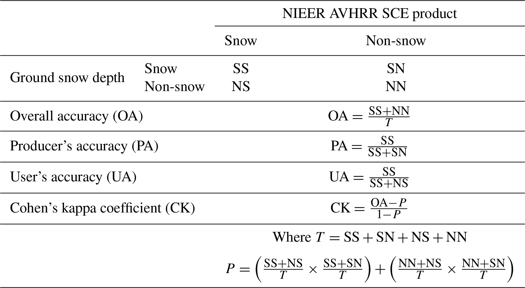
Note: SS, NN, NS, and SN are all numbers. SS represents the number of cases that AVHRR predicts snow, and the ground snow depth measures snow. NN represents the number of cases that AVHRR predicts non-snow, and the ground snow depth measures non-snow. SN represents the number of cases that AVHRR predicts non-snow, while the ground snow depth measures snow. NS represents the number of cases that AVHRR predicts snow, while the ground snow depth measures non-snow.

4.2 Validation with ground snow-depth measurements

As mentioned above, we will use 38-year CMA ground snow-depth measurements at 191 stations to validate the new NIEER AVHRR SCE product. Table 8 presents an overview of validation results. The OA is up to 87.4 %. The value of PA (81.0 %) was close to the UA (81.3 %), which indicated that the algorithm sensibly performed a trade-off between the omission error (19.0 %) and commission error (18.7 %). In addition, the CK value was 0.717. According to the guidelines presented by Landis and Koch (1977), this would place the level of agreement as “substantial”. All reveal that on a whole the new NIEER AVHRR product is accurate and has a good agreement with measurements of CMA stations.

Table 8 A confusion matrix for NIEER AVHRR SCE maps versus ground snow-depth measurements.

To validate the stability and reliability of the NIEER AVHRR SCE product, Fig. 7 presents the four accuracy metrics' annual fluctuation over the past 38 years. The OA ranged within 80 %–90 %, the PA and UA ranged within 70 %–90 %, and the CK value ranged from 0.61 to 0.8. Several considerable annual fluctuations mainly occurred in 1993, 1994, and 2017, which were mainly caused by the poor quality of raw satellite data rather than the algorithm. In summary, the product maintained a higher precision with small annual fluctuations, which indicated the effectiveness and stability of the training framework with different thresholds before and after 2000.

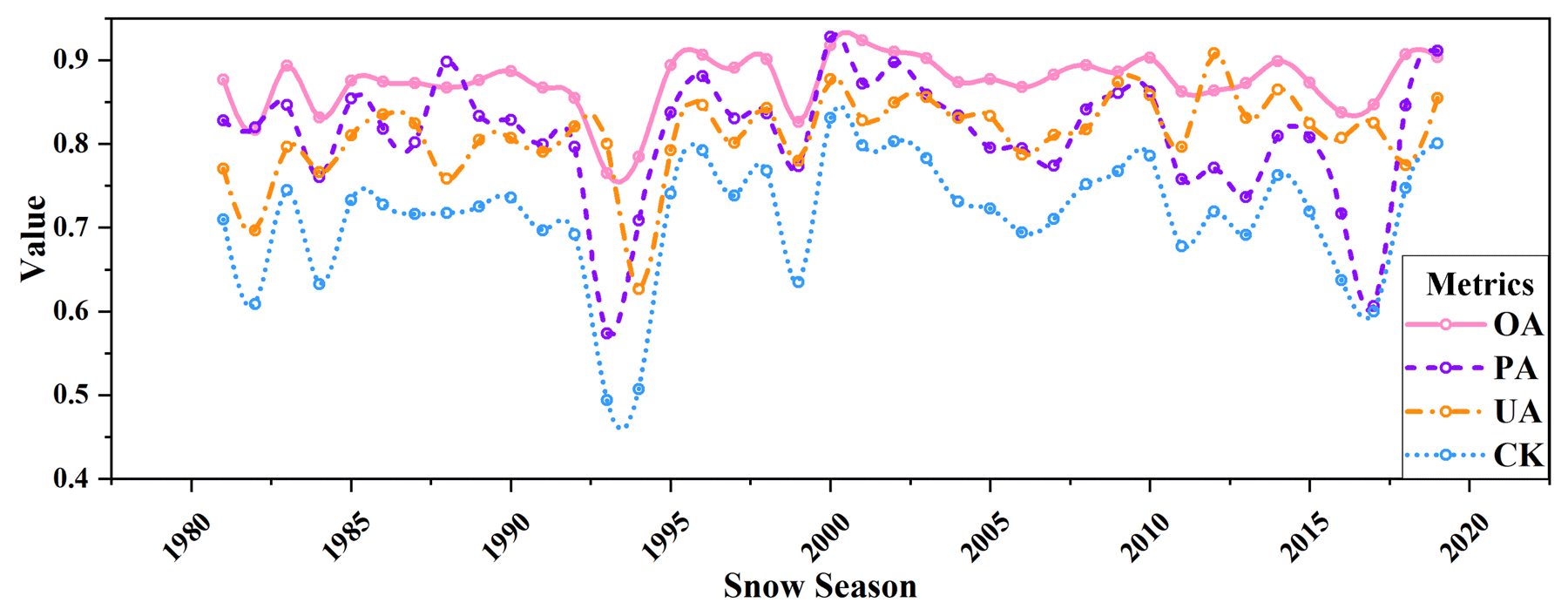
Figure 7 Accuracy fluctuations of NIEER AVHRR product based on ground snow-depth measurements in the past 38 years.

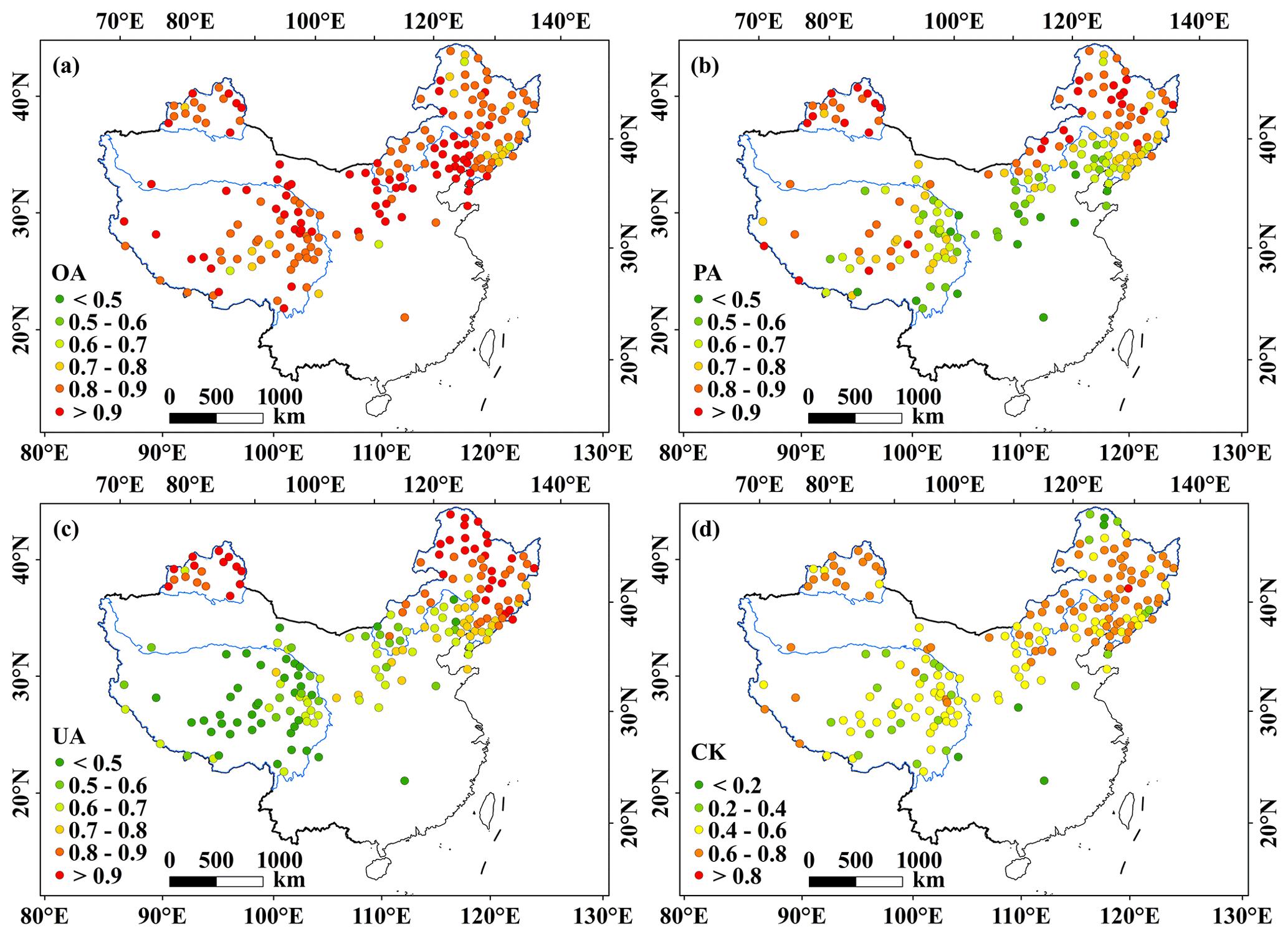
Figure 8 Point-based accuracy results of NIEER AVHRR product: (a) OA, (b) PA, (c) UA, and (d) CK. The snow depth of 191 climate stations used is provided by the China Meteorological Administration (CMA). OA, PA, UA, and CK represent overall accuracy, producer's accuracy, user's accuracy, and Cohen's Kappa coefficient.

Figure 8 further detailed accuracy metrics at each CMA station. From this figure, the OAs had higher values within 80 %–90 % at most stations across China, but PA, UA, and CK had low values with a clear spatial inconsistency. We found that the product performed well in north Xinjiang and the north of Northeast China where the stable snow was widely distributed. In contrast, the accuracy was relatively lower on the Qinghai–Tibet Plateau, Loess Plateau, in the northeast of Inner Mongolia, and in the south of Northeast China, where snowpack may be instable due to patchy snow-cover features, rugged terrains, or rapid melt even in winter.

4.3 Validation with Landsat-5 TM SCE maps

The measurements from CMA stations can provide time-continuous validation. However, such a “point-to-area” evaluation method also ignores the heterogeneity within pixels (Huang et al., 2011). The snow condition of an individual CMA station may not represent the larger area viewed by AVHRR. The “area-to-area” method using higher-resolution images has pointed out a good way to assess the snow spatial distribution of the AVHRR SCE product.

In the study, nine Landsat-5 snow maps were used to further evaluate the NIEER AVHRR product. Table 9 gives the validation results of our maps versus the Landsat-5 TM SCE maps. The OA was as high as 87.3 %. The high UA and low PA revealed that the product has a slight tendency to underestimate the snow cover extent. The CK value (0.695) of the area-to-area method also demonstrated “substantial” agreement, which was close to that of ground measurements validation (0.717). Therefore, no matter from either point of view (ground measurements) or area of view (Landsat-5 SCE maps), the NIEER AVHRR product is accurate. In general, the NIEER AVHRR SCE product is promising to better serve the climatic and other related studies in China.

Table 9 The accuracy of NIEER AVHRR SCE maps versus Landsat-5 TM SCE maps. C1–C8 denotes the different Landsat-5 TM SCE.

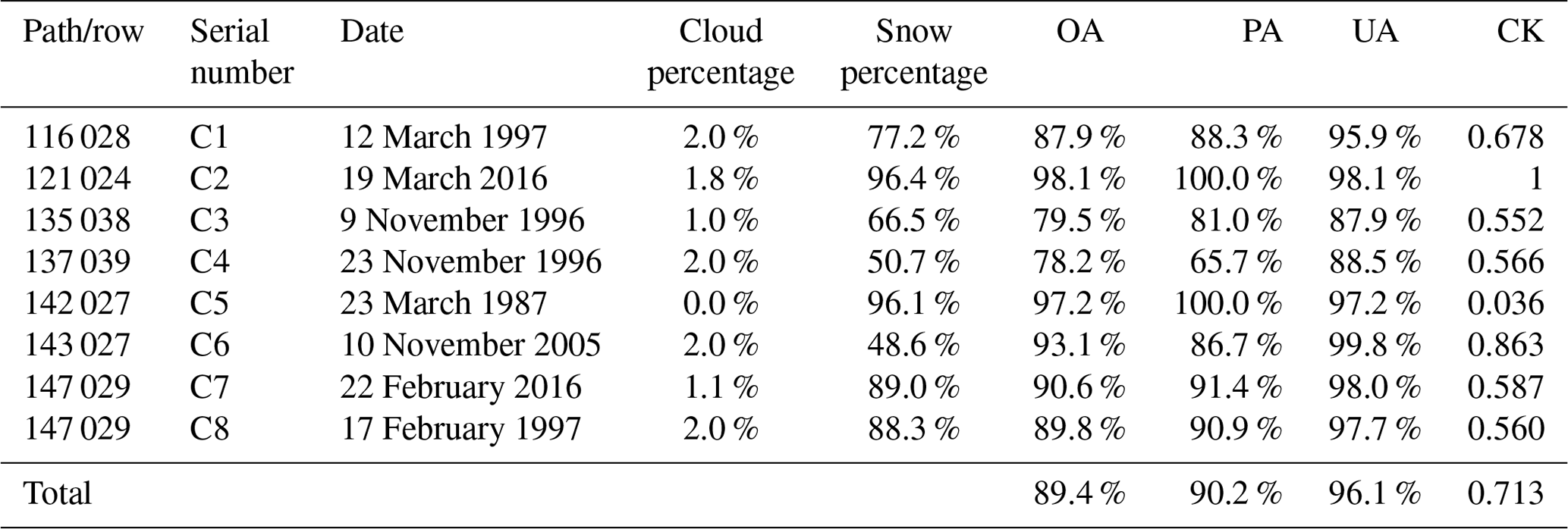
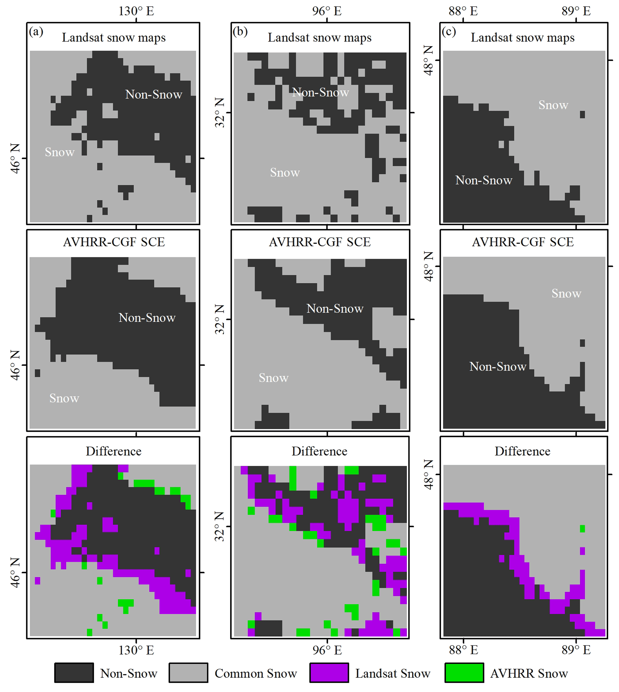
Figure 9 Comparison of Landsat reference images with NIEER AVHRR SCE images. Panel (a) is located in Northeast China on 12 March 1997, panel (b) is located in Qinghai–Tibet Plateau on 9 November 1996, and panel (c) is located in north Xinjiang on 10 November 2005.

Figure 9 further displays three intuitional examples demonstrating the detailed difference between NIEER AVHRR SCE maps and Landsat-5 SCE reference maps. The three images (serial numbers C1, C5, and C8) were located in Northeast China, the Qinghai–Tibet Plateau, and north Xinjiang, respectively. It was clear that the NIEER AVHRR SCE maps agree much better with higher-resolution snow maps in a wide range of snow-covered areas. However, in the boundaries of snow-covered areas, the NIEER AVHRR SCE maps failed to identify most snow pixels in the Landsat-5 SCE maps, which could be explained by the low ability of our product to detect low fractional snow-covered pixels.

5 Discussion

5.1 Uncertainties of the NIEER AVHRR SCE product

The validation based on both CMA stations and Landsat TM images indicated that the NIEER AVHRR SCE product performs well for large and deep snow cover. To explore the uncertainties of our product in the thin snow-covered areas, we set different snow-depth (SD) thresholds based on CMA measurements to further evaluate the NIEER AVHRR SCE product. Figure 10 shows the accuracy metrics of the product under different SD thresholds (SD ≥ 1 cm, SD ≥ 2 cm, SD ≥ 3 cm, SD ≥ 4 cm, and SD ≥ 5 cm).

Figure 10 Histogram of accuracy results of NIEER AVHRR SCE product under different snow-depth thresholds.

The results showed that the OA, UA, and CK values of the product decreased with increasing SD thresholds, while the PA values of the product increased with the increase in SD threshold. As SD increased, the UA presented a sharply decreasing trend, and PA presented a slightly increasing trend. On a whole, OA and CK values showed a significant decreasing trend. We can see our algorithm performed well at lower SD thresholds, which indicated the product has a better recognition ability for shallow snow.

Figure 11 Histogram of accuracy results of NIEER AVHRR SCE product in different snow periods, including accumulation period, stable period, and melting period.

Table 10 The confusion matrix and accuracy results of NIEER AVHRR and JASMES SCE products based on snow-depth measurements from CMA. OA, PA, UA, and CK.

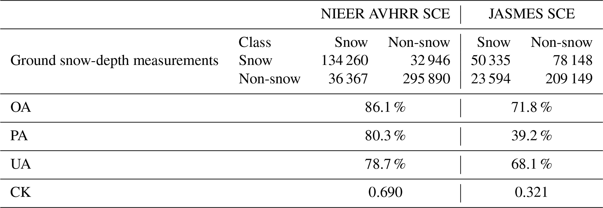
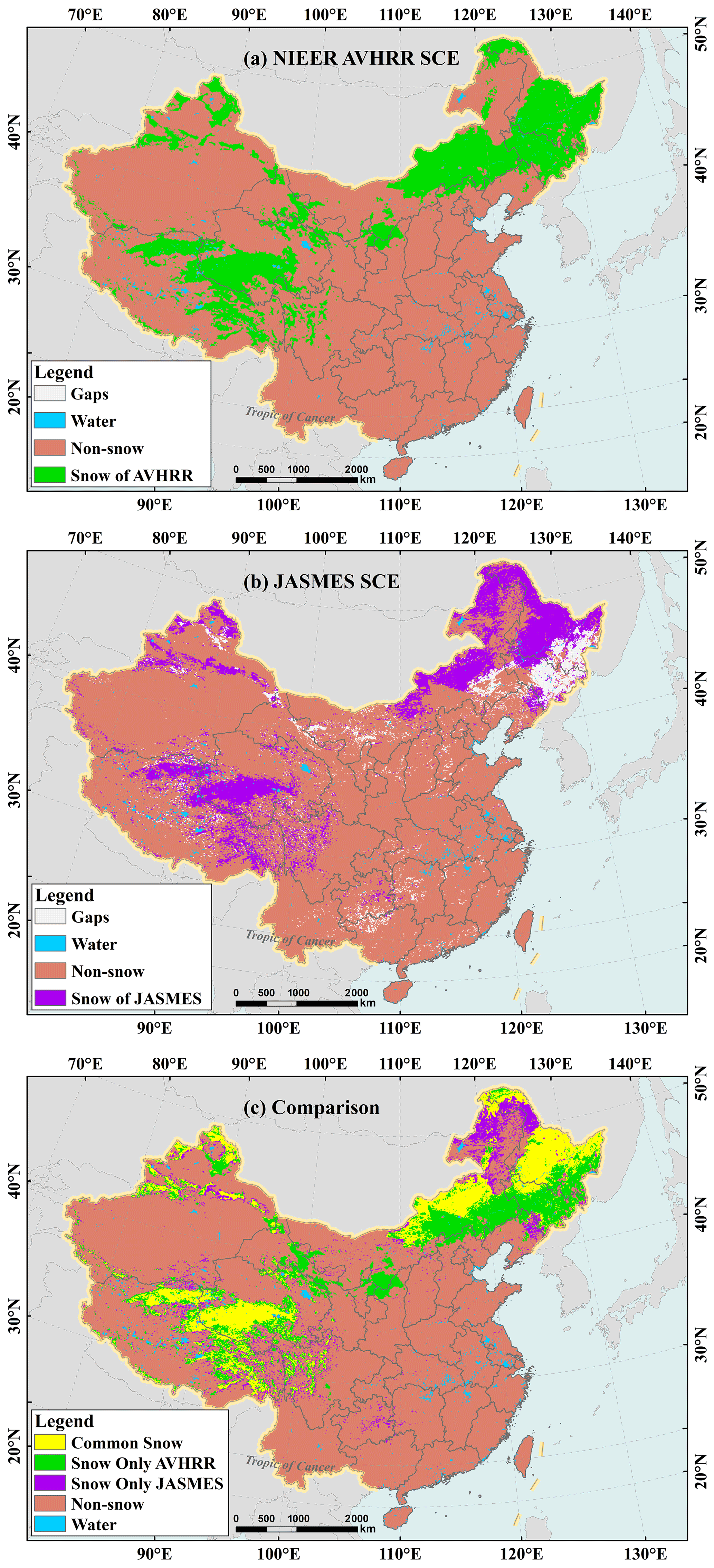
Figure 12 Comparison of snow cover maps between the NIEER AVHRR and JASMES SCE map over mainland China on 15 November 1985. Panel (a) is the NIEER AVHRR SCE map, panel (b) is the JASMES SCE map, and panel (c) is the comparison between the two snow maps.

Table 11 The description of NIEER AVHRR SCE product.

According to the snow cover temporal distribution feature in China, three seasonal snow periods were defined, i.e., the snow accumulation period, stable snow period, and snow melting period. The snow accumulation period is November. The stable snow period ranges from the beginning of December of the year to the end of February, and the snow melting period is March. Figure 11 presents the accuracy results of the NIEER AVHRR SCE product in different snow periods. The OAs of the accumulation period (87.7 %), stable period (86.7 %), and melting period (89.0 %) showed a similar response. However, the PAs, UAs, and CK values of the accumulation and melting periods were markedly lower than those of the stable snow period. The product had the highest omission errors (29.5 %) during the accumulation period because of the mixed pixels in the early snowfall seasons, while the product had the highest commission error (30.3 %) during the melting period due to the influence of wet snow.

5.2 Comparison of NIEER AVHRR and JASMES SCE products

To more objectively assess our product, we compared the NIEER AVHRR SCE product with JASMES SCE product. Since the JASMES SCE product was only generated by AVHRR data from 1981 to 1999, comparisons were made against the same ground snow-depth reference measurements in 19 snow seasons (1981–1999). Table 10 lists the comparison of the accuracy metrics. Our product performed well, with OA, PA, UA, and CK values of 86.1 %, 80.3 %, 78.7 %, and 0.690, respectively. The JASMES SCE products performed much worse, with total OA, PA, UA, and CK values amounting to 71.8 %, 39.2 %, 68.1 %, and 0.321, respectively. It means that our product clearly outperforms the JASMES product. Relative to the JASMES SCE product, the NIEER AVHRR OA increased approximately 15 %, the omission error dropped from 60.8 % to 19.7 %, the commission error dropped from 31.9 % to 21.3 %, and the CK value increased by more than 114 %. The JASMES product markedly underestimated the snow in China. In addition, there were about 50 000 validation samples in our product and only about 36 000 SD measurements in that of the JASMES product. Thus, our product should fill more gap pixels than JASMES. On the whole, the snow and cloud detection algorithm and the gap-filling strategy of our product performed better than those of JASMES.

To better figure out the spatial distribution difference between the two sets of products, comparison maps were constructed for 15 November 1985. Figure 12 presents the two SCE maps and their difference. There were significant differences in mapped snow extent between the two maps in the three major seasonal snow regions in China, i.e., north Xinjiang, Northeast China, and the Qinghai–Tibet Plateau. Our product mapped more snow in north Xinjiang, the Qinghai–Tibet Plateau, and the non-forest area in the northeast of China than JASMES. The most considerable discrepancy occurred on the Qinghai–Tibet Plateau where our product identified more snow-covered areas than JASMES. JASMES maps had more snow in the forested area of Northeast China than our product. Three improvements contributed to this phenomenon. Firstly, the snow algorithm proposed improved snow discrimination accuracy and reduced omission errors largely. Secondly, the cloud detection algorithm effectively improved the cloud–snow confusion, which identified the snow pixels that were misidentified as clouds pixels in the JASMES. Thirdly, the gap-filling strategy provided complete spatial coverage of snow cover.

6 Data availability

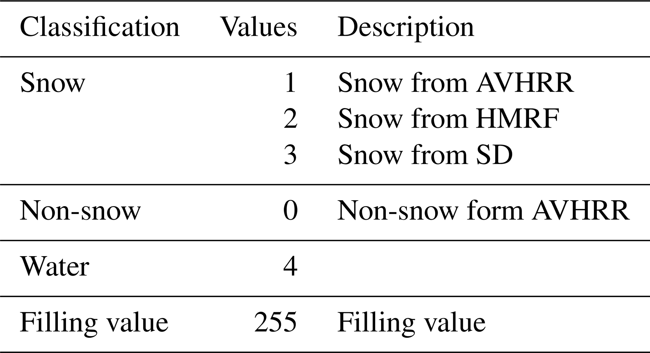
The NIEER AVHRR SCE product was named in the manner of NIEER_GF AVHRR SCE_yyyymmdd_DAILY_5km_V01 (V01 denotes the first version). It has a spatial resolution of 5 km and a daily temporal resolution. It spans latitude 16–56^∘ N and longitude 72–142^∘ E and now is freely accessible at https://doi.org/10.11888/Snow.tpdc.271381 (Hao et al., 2021). Detailed information on the product is listed in Table 11. The values in the product are classified as non-snow (0), snow from AVHRR (1), snow from HMRF (2), snow from SD (3), water (4), and filling value (255).

7 Conclusions

In this study, a daily AVHRR SCE product with a spatial resolution of 5 km across China's mainland from 1981 to 2019 has been generated by the snow research team in the NIEER, Chinese Academy of Sciences. The NIEER AVHRR SCE product used a multi-level decision tree algorithm for cloud and snow discrimination and an improved GF technique. The product was validated using snow-depth measurements provided by the China Meteorological Administration and higher-spatial-resolution SCE maps derived from Landsat-5 TM.

The OA of the NIEER AVHRR product was 87.4 %, a high accuracy, while the PA and UA were 81.0 % and 81.3 %, respectively. The PA and UA were similar, showing that the algorithm of the NIEER AVHRR product performed a trade-off between commission and omission errors. The CK value was 0.717, which indicated that the product had an agreement level of “substantial”. Considering the limitations of point-to-area validation, the overall OA, PA, UA, and CK values were 87.3 %, 86.7 %, 95.7 %, and 0.695, respectively, using area-to-area method compared to Landsat 5 TM, which showed the same trend of accuracy as the point validation. Therefore, no matter from either point of view or area of view, our AVHRR SCE product has high accuracy.

The performance of the NIEER AVHRR product in China was compared with the existing JASMES AVHRR SCE product. The OA, PA, UA, and CK value of the NIEER product were 86.1 %, 80.3 %, 78.7 %, and 0.690, and those of JASMES were 71.8 %, 39.2 %, 68.1 %, and 0.321. Compared with the JASMES product, the NIEER product OA increased approximately 15 %, the omission error dropped from nearly 60 % to 19.7 %, the commission error dropped from 31.9 % to 21.3 %, and the CK value increased by more than 114 %. Accordingly, the NIEER AVHRR product had a higher accuracy than the JASMES product. Furthermore, the NIEER product provides a completely gap-free product for China, permitting its wide applications.

Finally, we assessed the behavior of the NIEER AVHRR product during the snow accumulation, stable snow, and melting periods. The SCE performed best during the stable period, and the product was more accurate in the snow accumulation than the melting period. In general, the algorithm had a relatively high ability to identify shallower snow, but some uncertainties existed in patchy snow areas, regarding thinner snow, and in rugged terrain areas. As a long-term record, the dataset will provide a valuable data source for analyzing the influence of climate changes on the cryosphere on multiple timescales.