the Creative Commons Attribution 4.0 License.
the Creative Commons Attribution 4.0 License.
 | 07 Sep 2021
ERA5-Land: a state-of-the-art global reanalysis dataset for land applications
Joaquín Muñoz-Sabater
Emanuel Dutra
Anna Agustí-Panareda
Clément Albergel
Gabriele Arduini
Gianpaolo Balsamo
Souhail Boussetta
Margarita Choulga
Shaun Harrigan
Hans Hersbach
Brecht Martens
Diego G. Miralles
María Piles
Nemesio J. Rodríguez-Fernández
Ervin Zsoter
Carlo Buontempo
Jean-Noël Thépaut
Framed within the Copernicus Climate Change Service (C3S) of the European Commission, the European Centre for Medium-Range Weather Forecasts (ECMWF) is producing an enhanced global dataset for the land component of the fifth generation of European ReAnalysis (ERA5), hereafter referred to as ERA5-Land. Once completed, the period covered will span from 1950 to the present, with continuous updates to support land monitoring applications. ERA5-Land describes the evolution of the water and energy cycles over land in a consistent manner over the production period, which, among others, could be used to analyse trends and anomalies. This is achieved through global high-resolution numerical integrations of the ECMWF land surface model driven by the downscaled meteorological forcing from the ERA5 climate reanalysis, including an elevation correction for the thermodynamic near-surface state. ERA5-Land shares with ERA5 most of the parameterizations that guarantees the use of the state-of-the-art land surface modelling applied to numerical weather prediction (NWP) models. A main advantage of ERA5-Land compared to ERA5 and the older ERA-Interim is the horizontal resolution, which is enhanced globally to 9 km compared to 31 km (ERA5) or 80 km (ERA-Interim), whereas the temporal resolution is hourly as in ERA5. Evaluation against independent in situ observations and global model or satellite-based reference datasets shows the added value of ERA5-Land in the description of the hydrological cycle, in particular with enhanced soil moisture and lake description, and an overall better agreement of river discharge estimations with available observations. However, ERA5-Land snow depth fields present a mixed performance when compared to those of ERA5, depending on geographical location and altitude. The description of the energy cycle shows comparable results with ERA5. Nevertheless, ERA5-Land reduces the global averaged root mean square error of the skin temperature, taking as reference MODIS data, mainly due to the contribution of coastal points where spatial resolution is important. Since January 2020, the ERA5-Land period available has extended from January 1981 to the near present, with a 2- to 3-month delay with respect to real time. The segment prior to 1981 is in production, aiming for a release of the whole dataset in summer/autumn 2021. The high spatial and temporal resolution of ERA5-Land, its extended period, and the consistency of the fields produced makes it a valuable dataset to support hydrological studies, to initialize NWP and climate models, and to support diverse applications dealing with water resource, land, and environmental management.
The full ERA5-Land hourly (Muñoz-Sabater, 2019a) and monthly (Muñoz-Sabater, 2019b) averaged datasets presented in this paper are available through the C3S Climate Data Store at https://doi.org/10.24381/cds.e2161bac and https://doi.org/10.24381/cds.68d2bb30, respectively.
- Article
(9152 KB) - Full-text XML
-
Supplement
(987 KB) - BibTeX
- EndNote


The land surface state plays a crucial role in the coupled Earth system, especially on seasonal to interseasonal predictability and climate projections (Koster et al., 2004). The development of land surface models has greatly benefited from offline simulations to isolate the role of different land surface processes and to increase the performance of hydrological and thermodynamic variables. Land surface models were initially used in offline mode for model development with early intercomparison studies driven by either in situ observations (Henderson-Sellers et al., 1995; Etchevers et al., 2004) or global reanalysis datasets (Dirmeyer et al., 1999). More recently, multi-model intercomparison studies and datasets focusing on water resources monitoring (Harding et al., 2011; Schellekens et al., 2017) or climate modelling (van den Hurk et al., 2016; Krinner et al., 2018) have gained significant visibility. Offline simulations remain attractive due to their computational affordability and the needs that follow from the rapid evolution of land surface models (Pitman, 2003; Vereecken et al., 2019; Boussetta et al., 2021).
A key advantage of using offline land surface estimates is their temporal consistency, unlike in the case of coupled land–atmosphere predictions (e.g. operational weather forecasts) that experience frequent updates. Atmospheric reanalyses also provide such a consistency. However, atmospheric reanalysis can be affected by systematic biases, in particular in precipitation, which has led to the development of bias correction methodologies (Weedon et al., 2011; Reichle et al., 2017). Land data assimilation systems (LDASs) also provide an important component of reanalyses, which can mitigate model errors and enhance the representation of the land surface state in regions and periods with available observations (Albergel et al., 2017). However, this can also result in temporal and spatial inconsistencies (e.g. due to changing observations' availability) as well as limitations in the closure of the surface water budget (Zsoter et al., 2019). Examples of existing global offline datasets are the Global Offline Land-surface Data-set (GOLD) (Dirmeyer and Tan, 2001), MERRA-Land (Reichle et al., 2011), and ERA-Interim/Land (Balsamo et al., 2015). The latter was motivated by important updates to the European Centre for Medium-Range Weather Forecasts (ECMWF) land surface scheme introduced in the operational forecasting model in 2006, when the production of ERA-Interim started. These changes embedded in ERA-Interim/Land provided seasonal forecasting with more accurate and consistent land initial conditions. Compared to atmospheric reanalysis, offline land surface reanalyses can be produced faster and at more affordable computational cost. An arguable disadvantage compared to high-resolution Earth observation data is the lack of small-scale heterogeneity found in offline model-only based estimates. However, observational datasets suffer from temporal and spatial gaps, and only a few land variables are directly “observable”, so complex algorithms that blend observations and model output are needed to retrieve a complete estimate of land variables. Furthermore, advances in land surface modelling and the increase of computational resources now make it feasible to run offline models at finer resolutions than traditionally possible. Therefore, offline global simulations are a valuable way to ensure continuity and completeness of the land surface fields, which are two important aspects to foster research at continental scales in climate studies.
Although the development of offline model estimates has been motivated mainly by climate and weather research, new user requirements are constantly emerging in society. The effects of climate change are pushing different economic sectors to implement novel adaptation strategies to adjust to the new reality. For example, crop production is already being affected by increasing temperatures and decreased water availability (Lobell et al., 2011; Wheeler and von Braun, 2013; Zhao et al., 2017). This may induce changes to traditional watering crop strategies, harvesting periods, pest management, or even crop culture replacements. Likewise, insurance (and reinsurance) companies need reliable historical data to assess the risk of severe droughts or flooding (Tadesse et al., 2015; Jensen and Barrett, 2016), in particular for smallholder agriculture. For public and private stakeholders, offline land surface datasets can provide complementary information needed to support decision makers.
This paper documents the new land component of the fifth generation of European ReAnalysis (ERA5), hereafter referred to as the ERA5-Land dataset (Muñoz-Sabater, 2019a). Unlike ERA-Interim/Land, which was produced as a one-off single-simulation research dataset covering the period of 1979–2010, ERA5-Land is now an integral and operational component of the Copernicus Climate Change Service (C3S). This means, among others, that the production is guaranteed with timely updates and synchronized with ERA5 monthly updates. To investigate the added value of ERA5-Land, the latter was compared to two other operational reanalysis products: ERA5 and ERA-Interim (operational until 31 August 2019). This comparison also makes it possible to study the evolution of ECMWF operational reanalyses. ERA-Interim/Land was not included in the comparison as it was only available until 2010, and it was intended to be a research dataset. As a reference for the evaluation, in situ observations from different networks around the globe have been used for comparison to the reanalyses estimates. In addition, complementary global gridded model- or satellite-based datasets have been incorporated into the evaluation exercise. Improvements in ERA5 compared to ERA-Interim are mainly due to 10 years of additional research and development (R&D) in the use of satellite data in numerical weather prediction (NWP) and atmospheric modelling (Hersbach et al., 2020). Differences between ERA5 and ERA5-Land are not so obvious. They both share quite similar parameterizations of land processes; the main improvement of ERA5-Land is due to the non-linear dynamical downscaling with corrected thermodynamic input.
Section 2 describes the main steps of the methodology used to produce ERA5-Land; in Sect. 3, the data used to investigate the added value of ERA5-Land compared to ERA5 and ERA-Interim (mainly from the years 2000–2018) are described. Section 4 shows the results of the evaluation exercise, while information on access to the data is presented in Sect. 5. A discussion of the results and the conclusions is presented in Sect. 6, followed by perspectives for future updates in Sect. 7
ERA5-Land produces a total of 50 variables describing the water and energy cycles over land, globally, hourly, and at a spatial resolution of 9 km, matching the ECMWF triangular–cubic–octahedral (TCo1279) operational grid (Malardel et al., 2016). For a full list of the available fields in the ERA5-Land catalogue, see Table A2 in Appendix A. The production is conducted in three segments or streams. The reason is two-fold: (1) it allows the production of parallel streams, therefore accelerating the production and the public availability of the data; (2) the atmospheric forcing necessary to produce ERA5-Land is derived from ERA5, and thus the production needs the corresponding segment of ERA5 completed for the same time period. Figure 1 shows the different data streams designed in the production of ERA5-Land. The production started with data from the year 2001 (stream-1) aiming at making available firstly the most recent data, while the back extension from 1950 to 1980 (stream-3) is currently under production.
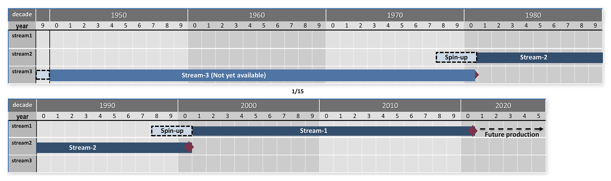
Figure 1Diagram of the production streams of ERA5-Land. The dark blue lines correspond to the data that have already been produced and are available through the C3S Climate Data Store. The light blue line corresponds to the back-extension period, and at the time of writing this paper is under production. The 3-year spin-up period for stream-1 and stream-2 is presented with dashed rectangles. Stream-3 has a 1-year spin-up (1949). The red diamond presents the end of each stream.
Each segment or stream is initialized with meteorological fields from ERA5. ERA5-Land does not assimilate observations directly. The observations influence the land surface evolution via the atmospheric forcing. Forcing air temperature, humidity, and pressure are corrected using a daily lapse rate derived from ERA5. After that, the land surface model is integrated in 24 h cycles providing the evolution of the land surface state and associated water and energy fluxes. In addition to the hourly data, monthly means are also computed (Muñoz-Sabater, 2019b). Figure 2 shows a diagram of the algorithm used for each 24 h production cycle. The most important components of the production algorithm are presented in the following subsections.
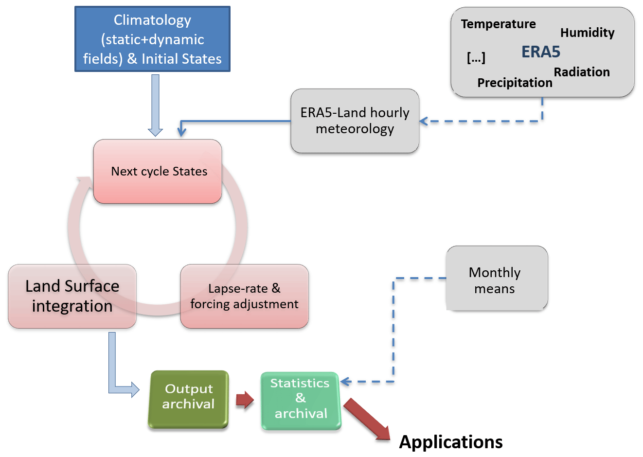
Figure 2Diagram of the algorithm used in the production of ERA5-Land. The land surface model is integrated in 24 h cycles using short-forecast meteorological forcing fields from ERA5.
2.1 Initialization
ERA5-Land is not produced as a single continuous simulation for the entire period. The production is conducted in three independent streams, as shown in Fig. 1. To avoid or minimize discontinuities between streams, a careful initialization procedure is needed for each of them. Particular attention must be given to variables carrying long memory. As an example, Fig. 3 shows time series of deep soil moisture in a band of latitude between 60 and 20∘ S, where the averaged annual soil moisture variability is low. This period includes several production streams of ERA5. ERA5 initialized each stream with ERA-Interim soil moisture initial conditions, which has a different climatology than ERA5. In ERA5, a 1-year spin-up was used for each production stream and it is normally long enough for atmospheric variables. However, it is not sufficient for deep soil moisture to reach equilibrium, which leads to discontinuities between two production streams, as shown in Fig. 3.
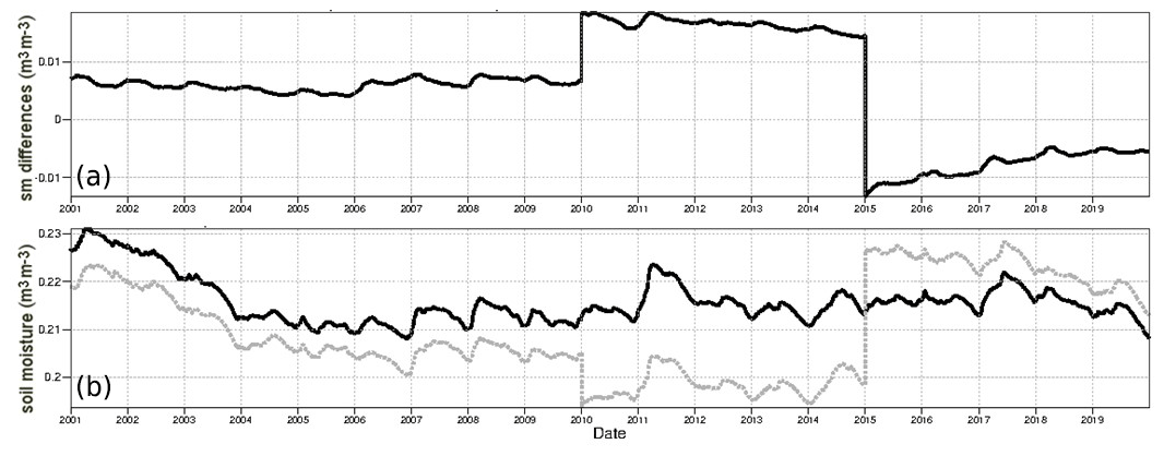
Figure 3(a) Mean differences between ERA5-Land and ERA5 soil moisture (sm) time series for the fourth soil layer of the Carbon Hydrology-Tiled ECMWF Scheme for Surface Exchanges over Land (CHTESSEL) land surface model (100–289 cm), averaged for the latitudes 60–20∘ S. The temporal resolution is 12 h. Panel (b) is the same as (a) but showing the raw time series of ERA5 (dashed light grey curve) and ERA5-Land (dark curve).
The strategy followed to initialize the ERA5-Land production stream starting in 2001 (stream-1) was to use the latest year of a long, prior ERA5 stream, and letting 3 further spin-up years to allow a long spin-up period (see Fig. 1). While this strategy provides satisfactory results for most continental masses around the world, discontinuities are still possible at areas with very low variability of soil moisture (deserts and polar regions). Particular attention was given to the treatment of permanent snow-covered regions. The current model formulation (as in ERA5) does not have an independent treatment of glaciers. Grid points with glaciers are assigned with a constant snow mass of 10 m. ERA5-Land streams are initialized on the 1 January, and a glacier mask is applied to snow mass to guarantee the correct spatial representation of glaciers. A threshold of 50 % of a grid box covered by ice is used, below which the snow depth keeps the value computed by the snow scheme of the land model. Values above the threshold assign a snow water equivalent value of 10 m. This condition is used to avoid grid points near glaciers with large unrealistic snow depth that result from the interpolation from ERA5 fields to ERA5-Land. For the stream starting in 1981 (stream-2), a long, prior ERA5 stream was not available. The strategy in this case was to initialize using a ERA5-Land climatology of 1 January for the period 2001–2018 and then allow the system to spin up for 3 years. A similar strategy was used to initialize the stream starting in 1950 (stream-3), but in this case a 1981–2010 climatology was used and only 1 spin-up year was feasible. The latter was limited by the availability of forcing data.
2.2 Static and climatological fields
As in ERA5, the land characteristics are described using several time-invariant fields. These consist of the land–sea mask, the lake cover and depth, the soil and vegetation type, and the vegetation cover. In addition, surface albedo and leaf area index are prescribed as monthly climatologies. The complete list of time invariant fields with their information source is provided in Table A1 of Appendix A.
2.3 Atmospheric forcing
ERA5-Land is driven by atmospheric forcing derived from ERA5 near-surface meteorology state and flux fields. The meteorological state fields are obtained from the lowest ERA5 model level (level 137), which is 10 m above the surface, and include air temperature, specific humidity, wind speed, and surface pressure. The surface fluxes include downward shortwave and longwave radiation and liquid and solid total precipitation. These fields are interpolated from the ERA5 resolution of about 31 km to ERA5-Land resolution of about 9 km via a linear interpolation method based on a triangular mesh. The atmospheric forcing built for ERA5-Land is hourly and consistent over the entire production period, and it is the result of the assimilation of a large number of conventional meteorological and satellite observations through a four-dimensional variational assimilation system (4D-Var) and simplified extended Kalman filter (SEKF) systems as described in Hersbach et al. (2020). Previous land reanalyses have included corrections to the precipitation forcing to address limitations of the precipitation fields of the atmospheric reanalysis. This is not the case in ERA5-Land mainly due to the (1) enhanced quality of ERA5 precipitation when compared with previous atmospheric reanalyses (e.g. Beck et al., 2019; Tarek et al., 2020; Nogueira, 2020) and (2) reduced dependencies on external data that would limit the near-real-time data availability. However, air temperature, humidity, and pressure are corrected for the altitude differences between ERA5 and ERA5-Land grids. This correction involves four steps: (i) relative humidity is computed from interpolated, uncorrected fields; (ii) air temperature is adjusted for the altitude differences using a daily environmental lapse rate (ELR) field derived from ERA5 lower troposphere temperature vertical profiles (Dutra et al., 2020); (iii) surface pressure is corrected for the altitude differences and correction of temperature; and (iv) specific humidity is computed using the corrected temperature and pressure assuming that there is no change in relative humidity. Dutra et al. (2020) present a detailed evaluation of this methodology comparing the use of a constant (time and space) ELR with daily ELR fields derived from ERA5. This methodology was shown to reduce the mean absolute error (MAE) of daily maximum temperature by 10 % and by 4 % for daily minimum temperature with respect to ERA5 when compared with 2941 stations over the western US. The importance of the ELR correction is shown in the orography map of the Alpine region around Switzerland in Fig. 4. ERA5 misses many of the highest Alpine peaks due to the coarser resolution. Taking into account these orographic differences is important for other land variables such as surface temperature. For instance, the middle and bottom rows show a more realistic spatial pattern of surface temperature in ERA5-Land, with a clear cold signal over the higher peaks. It is also remarkable to see how ERA5-Land is able to resolve lakes such as Geneva (Léman), Neuchâtel, and Constance. This is especially visible at 06:00 UTC, when the lake surface temperature is still significantly warmer than the land (Fig. 4f).
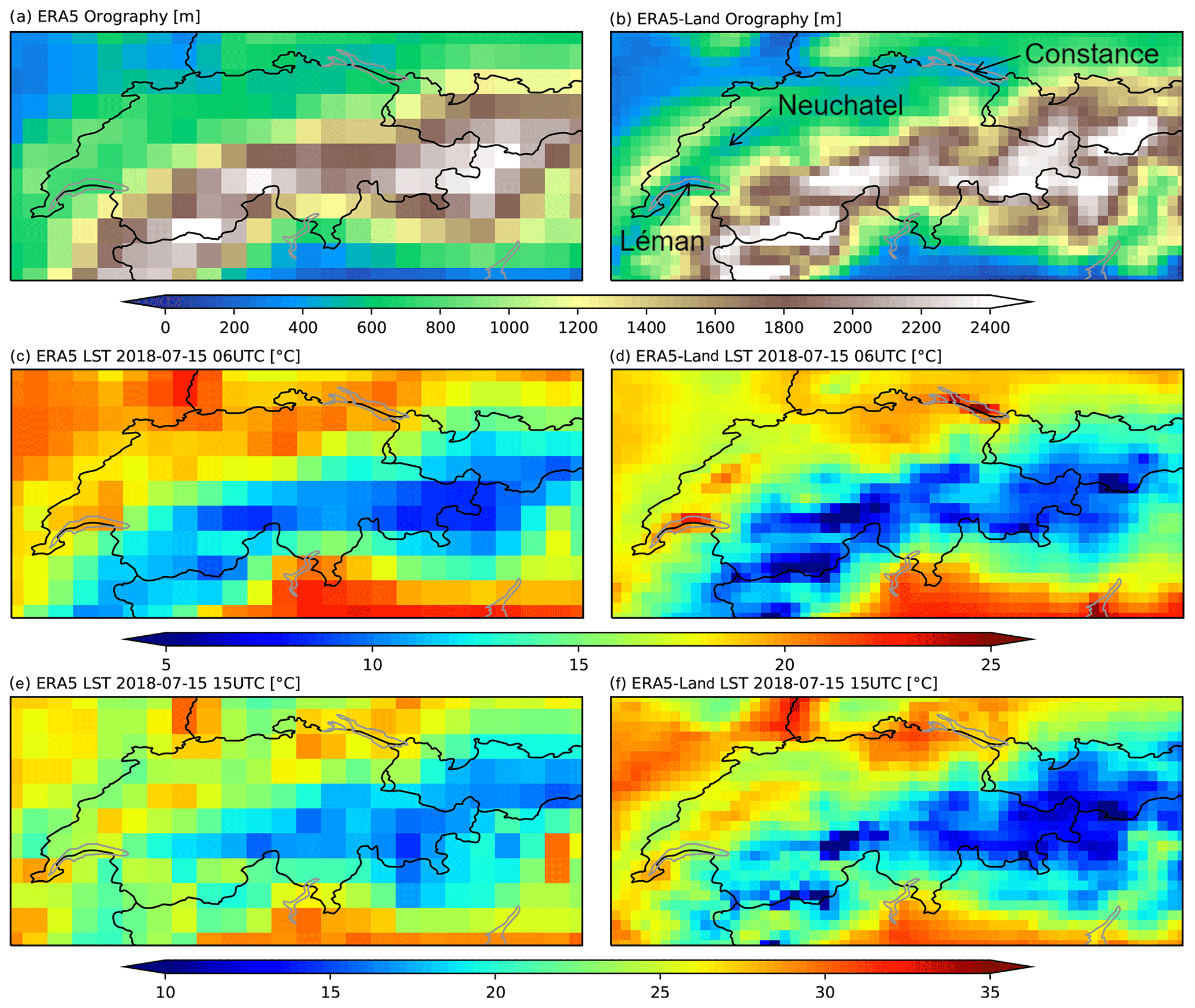
Figure 4ERA5 (a, c, e) and ERA5-Land (b, d, f) orography (a, b) of the Alpine region around Switzerland. Panels (c, d) and (e, f) show the ERA5 and ERA5-Land land surface temperature (LST) estimates on 15 July 2018 at 06:00 UTC (c, d) and 15:00 UTC (e, f), respectively. The locations of lakes Geneva (Léman), Neuchâtel, and Constance are indicated in panel (b).
2.4 Land surface model
The core of ERA5-Land is the ECMWF land surface model: the Carbon Hydrology-Tiled ECMWF Scheme for Surface Exchanges over Land (CHTESSEL). The main updates with respect to the land component of ERA-Interim are (a) a revised soil hydrology, introducing an improved formulation of the soil hydrologic conductivity and diffusivity (that now is variable as a function of soil texture) and surface runoff based on variable infiltration capacity (Balsamo et al., 2010); (b) a fully revised parametrization of the snow scheme, changing the hydrological and radiative properties of the snowpack (Dutra et al., 2010); (c) the introduction of a climatological seasonality of vegetation, in contrast to the fixed vegetation in ERA-Interim (Boussetta et al., 2013b); (d) a new scheme for bare soil evaporation, allowing soil moisture to reach values below the wilting point (Albergel et al., 2012); (e) introduction of a lake model to represent the thermodynamics of inland water bodies (Balsamo et al., 2012); and (f) a parametrization that allows the estimation of land carbon fluxes – net ecosystem exchange (NEE), gross primary production (GPP), and ecosystem respiration (Reco) – in a modular way with the Jarvis approach that computes the stomatal conductance without affecting the transpiration components (Boussetta et al., 2013a).
The land surface model version used in ERA5-Land was operational at ECMWF in 2018 with the model cycle Cy45r1. A detailed description of the model can be found in chapter IV of the Integrated Forecasting System (IFS) documentation (https://www.ecmwf.int/node/18714, last access: December 2020). Compared with the model version of ERA5, the differences are mostly technical, with the exception of (i) an updated parametrization of the soil thermal conductivity following Peters-Lidard et al. (1998) that takes into account the ice component in the case of frozen soil, (ii) a fix to improve conservation for the soil water balance, and (iii) rain over snow is accounted for and it does not accumulate in the snowpack. Potential evapotranspiration (PET) flux in ERA5 suffers from a bug present in IFS cycle 41r2 that affects PET computation over forests and deserts. This problem has been corrected in ERA5-Land, and unlike in ERA5, ERA5-Land includes PET in the portfolio of products. Given the importance of this variable for some applications, it is worth clarifying that PET is computed by making a second call to the surface energy balance assuming a vegetation type of crops and no soil moisture stress. In other words, evaporation is computed for agricultural land as if it is well watered and assuming that the atmosphere is not affected by this artificial surface condition. The latter may not always be realistic. Therefore, despite the fact that PET is meant to provide an estimate of irrigation requirements, one has to be cautious especially for arid conditions, since the method can give unrealistic results due to too-strong evaporation forced by dry air.
To evaluate the quality of the ERA5-Land fields, several key variables of the water and energy cycles were selected and compared to available in situ observations and to a series of reference datasets. Note that the list of evaluated variables and reference datasets is not exhaustive and was based on factors such as availability of data at the time of the evaluation. ERA-Interim and ERA5 reanalyses were included in the comparison, aiming at showcasing the progress of operational reanalyses at ECMWF. The variables evaluated are soil moisture, snow depth, lake surface water temperature and river discharge for the water cycle, the sensible and latent heat fluxes (the latter also a component of the water cycle), the Bowen ratio, and skin temperature for the energy cycle. This section describes the supporting datasets used in the evaluation exercise and the metrics employed to assess the quality of ERA5-Land fields.
3.1 ERA-Interim
ERA-Interim (Dee et al., 2011) is the former ECMWF reanalysis providing estimates for the atmosphere, ocean waves, and land surface. It had supported scientific progress during the previous decade and is still widely used today by the scientific community. It includes information on multiple land and atmospheric variables, and it is available from January 1979 to August 2019. It used the IFS version Cy31r2 (more detailed information available at https://www.ecmwf.int/en/publications/ifs-documentation, last access: 27 August 2021), corresponding to the IFS 2006 release, with a spatial horizontal resolution of about 80 km and 60 levels in the vertical from the surface to 0.1 hPa. The system includes a 4D-Var system (Rabier et al., 2000) providing analyses fields at a temporal resolution of 6 and 3 h for short-forecast fields (like for precipitation and fluxes). The main difference between the land component of ERA-Interim and those of both ERA5 and ERA5-Land is that the former is based on TESSEL (van den Hurk et al., 2000), which is considered the precursor of the current CHTESSEL scheme. In ERA-Interim, the soil moisture and soil temperature analyses are based on a local optimal interpolation scheme (Mahfouf, 1991; Douville et al., 2000) that assimilates surface synoptic (SYNOP) observations of temperature and relative humidity at screen level (2 m). The snow depth analysis is independent of the soil wetness and is based on a Cressman analysis that assimilates SYNOP snow reports and snow-free satellite observations (Drusch et al., 2004).
3.2 ERA5
ERA5 is the latest comprehensive ECMWF reanalysis and has replaced ERA-Interim. It is based on a version of the ECMWF IFS (Cy41r2) that was operational in 2016. ERA5 provides hourly estimates of the global atmosphere, land surface, and ocean waves from 1950 and is updated daily with a latency of 5 d. Its state estimates are based on a high-resolution (HRES) component at a horizontal resolution of 31 km and with 137 levels in the vertical spanning from the surface up to 0.01 hPa. Information on uncertainties in these are provided by a 10-member ensemble of data assimilations (EDA) at half the horizontal resolution. Both the HRES and EDA ERA5 data assimilation use background-error estimates that utilize the output from the EDA. The land component of ERA5 is, like ERA5-Land, based on the CHTESSEL model, though at a resolution of 31 km rather than 9 km. ERA5 uses new analyses of sea-surface temperature and sea-ice concentration, variations in radiative forcing derived from CMIP5 specifications, and various new and reprocessed observational data records.
The data assimilation system consists of an incremental 4D-Var component (Courtier et al., 1994) for upper-air and near-surface components, an ocean-wave optimal interpolation scheme, and a dedicated LDAS. The LDAS comprises a two-dimensional optimal interpolation scheme for the analysis of screen-level 2 m temperature and relative humidity, and for snow (depth and density), a point-wise simplified extended Kalman filter (de Rosnay et al., 2013) for three soil moisture layers in the top 1 m of soil, and a one-dimensional optimal interpolation for soil, ice, and snow temperature. Details of the ERA5 configuration are given in Hersbach et al. (2020), which also contains a basic evaluation of characteristics and performance for the segment from 1979 onward. The performance of the component from 1950 to 1978, the back extension which was made available later, is described in Bell et al. (2021), and a detailed analysis for surface temperature and humidity is provided by Simmons et al. (2021). Technical details are also provided in the online documentation (https://confluence.ecmwf.int/display/CKB/ERA5:+data+documentation, last access: 23 August 2021).
Table 1Overview of the main characteristics of ERA-Interim, ERA5, and ERA5-Land.
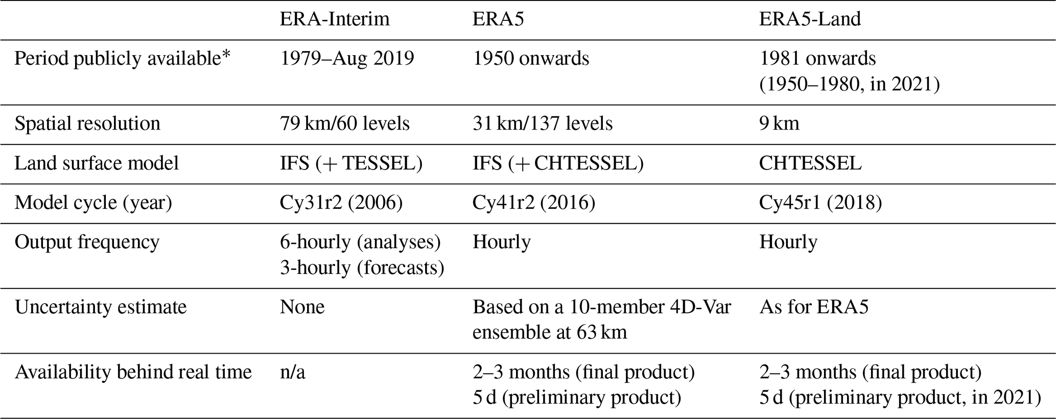
* Availability at the time of submitting this paper. n/a – not applicable.
Both ERA5 and ERA5-Land are produced as part of the Copernicus Climate Change Service that ECMWF operates on behalf of the European Commission and are available from the C3S Climate Data Store (CDS). ERA5 and ERA5-Land have a large and diverse user base (more than 40 000 users at the end of 2020). Table 1 summarizes the main characteristics of ERA-Interim, ERA5, and ERA5-Land.
3.3 Soil moisture
To evaluate the quality of the soil moisture estimates from the various reanalyses, a large number (>800) of in situ sensors in the period 2010 to 2018, many providing hourly measurements, were used. These sensors belong to the networks that are listed in Table 2. The networks are located in North America, Europe, Africa, and Australia, and all the observations were retrieved from the International Soil Moisture Network (Dorigo et al., 2011, 2021). Three reanalysis soil layer estimates were compared to measurements by sensors at three different depths. ERA5 and ERA5-Land top layer soil moisture estimates (0–7 cm) were compared to in situ sensors at 5 cm depth in North America, Africa, Europe, and Australia. A more in-depth study was performed in North America, where most of the sensors are located. For this region, surface soil moisture from ERA-Interim was also evaluated. In addition, ERA5, ERA5-Land, and ERA-Interim soil moisture for the second (7–28 cm) and third layers (28–100 cm) were evaluated against in situ measurements at 20 and 50 cm depth, respectively. In situ measurements were compared to the closest grid point of the ERA5, ERA5-Land, and ERA-Interim grids if the closest grid point was not farther than the respective model resolution. In situ time samples were selected in a ±1 h window with respect to the reanalysis timestamp. If several observations were retrieved in a single window, the average was computed. In order to consider an observed time series suited for the comparison, a minimum of 150 samples was required for the study period. To remove the seasonal cycle, anomaly time series were also computed. The soil moisture anomaly values at time t (SMAN(t)) were computed from the original time series (SM(t)) computing the mean () and the standard deviation (σSM) of soil moisture a ±17 d window as follows:
The following metrics were computed between the reanalyses estimates and the in situ time series: the standard deviation of the difference (STDD, equivalent to the unbiased RMSD), the bias, and the Pearson correlation coefficient (R). The latter was also computed for the anomaly time series (RAN). The results were grouped per continent and their distribution presented in box plots. Values are considered outliers if they are greater than or less than , with q25 and q75 the 25th and 75th percentiles, respectively.
Schaefer et al. (2007)Bell et al. (2013)Leavesley et al. (2008)Moghaddam et al. (2010b)Zacharias et al. (2011)Calvet et al. (2007)Ikonen et al. (2016)Martínez-Fernández and Ceballos (2005)Tallec et al. (2015)Lopez-Baeza et al. (2009)Bircher et al. (2012)Lafore et al. (2010)Tagesson et al. (2015)Young et al. (2008)Smith et al. (2012)Table 2In situ measurement networks used to evaluate soil moisture. The different columns contain the region and the name of the network, the depths of the probes used, and the bibliographic reference to the network.

3.4 Snow
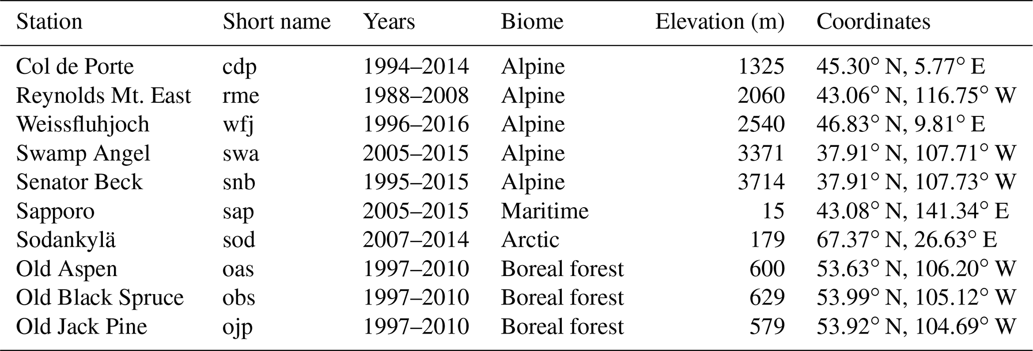
Snow depth estimates from reanalyses were compared to two sets of observational data. The first one comprises 10 sites distributed among North America, Europe, and Japan. They were selected as reference sites to evaluate cold processes by models participating in the Earth System Model – Snow Model Intercomparison Project (ESM-SnowMIP) (Krinner et al., 2018; Ménard et al., 2019). These sites provide benchmarking data for cold processes in maritime, Alpine, and taiga types of snow cover and on different types of climates. Table 3 presents these stations.
Table 3List of ESM-SnowMIP sites used for the evaluation of the snow parameters, adapted from Krinner et al. (2018).
The second dataset is retrieved from the Global Historical Climatology Network-Daily (GHCN-daily) (Menne et al., 2012b) from 1 July 2010 to 30 June 2018. The version used is v3.24 (Menne et al., 2012a). This network integrates thousands of land surface stations across the globe. The daily observed snow depth product was compared to the daily averaged snow depth estimates from ERA-Interim, ERA5, and ERA5-Land at 00:00 and 12:00 UTC. To compare the reanalysis data with the snow depth observations, the prognostic snow water equivalent (SWE, in units of m water equivalent) and snow density (ρsnow, kg m−3) from the reanalysis were combined to compute the actual snow depth (SD, m):
where ρwater=1000 kg m−3 is the reference density of the water. The GHCN observations were only considered if snow depth values were positive and missing values were lower than 50 % of the recorded time series. Also stations where the snow depth reported is lower than 1 cm in more than 5 % of the total number of days were removed. Finally, stations located in coastal areas with more than 50 % water in the pixel and on permanent snow area (glaciers) were removed. More than 6000 stations passed the quality filters, and their locations can be found in Fig. 9. The quality of the snow depth from the reanalyses was evaluated at the hemispheric scale by computing the mean bias (here defined as reanalysis estimate minus in situ observation) and root mean square error (RMSE) for the months between December and June of the 2010–2018 period.
3.5 Lakes
In 2015, the CHTESSEL land surface scheme of the operational IFS introduced a lake tile, which represents lakes, reservoirs, rivers, and coastal (subgrid) waters, and is based on the FLake (Fresh-water Lake) model of Mironov et al. (2010a). FLake is a one-dimensional model, which uses an assumed shape for the lake temperature profile including the mixed layer (uniform distribution of temperature) and the thermocline (its upper boundary located at the mixed-layer bottom, and the lower boundary at the lake bottom). To run FLake, the lake location (or fractional cover), lake depth (most important parameter, preferably bathymetry), and lake initial conditions are required. For the best performance, lake depth should be updated with the latest available information to ensure that depths are close to observed values, as overestimated depths can be blamed for cold biases in summer temperatures or lack of ice. The state of lakes in FLake is described by seven prognostic variables: mixed-layer temperature, mixed-layer depth, bottom temperature, mean temperature of the water column, shape factor (with respect to the temperature profile in the thermocline), temperature at the ice upper surface, and ice thickness. In this paper, the lake surface water temperature (LSWT) estimates from the FLake model embedded in ERA5 and ERA5-Land were compared to in situ observations from three different sources of data, during ice-free periods:
-
The Alqueva reservoir in Portugal, from the Portuguese University of Évora, provided hourly data from 2017 and 2018. In addition, daily averaged values were also computed.
-
In total, 27 Finnish lakes monitored by Finnish Environment Institute (SYKE) provided daily data (one measurement per day at 08:00 LT) from 2000 to 2016. In addition, summer month (June, July, and August) average values were calculated.
-
Summer month average values were provided from the global inventory “Globally distributed LSWT collected in situ and by satellites; 1985–2009” (https://portal.edirepository.org/nis/mapbrowse?packageid=knb-lter-ntl.10001.3, last access: 29 August 2021). In total, there were 348 lakes over the globe with in situ data for 15 years (1995–2009).
Figure 5 provides the location of all the sources of in situ data used in this study. Considering the above observations as the truth, the MAE of ERA5 and ERA5-Land LSWT estimates was computed. The significance of these results was tested using the Kruskal–Wallis test by ranks. In addition, the bias distribution was also calculated and presented in 2-D bar graphs. It should be noted that the Alqueva reservoir and the 27 Finnish lake depths were verified (in situ vs. operational values) and are in good agreement; the lake depths provided by the “Globally distributed LSWT collected in situ and by satellites; 1985–2009” global inventory were only randomly verified (e.g. by comparison with scientific publications), which might add some uncertainty when interpreting the results.
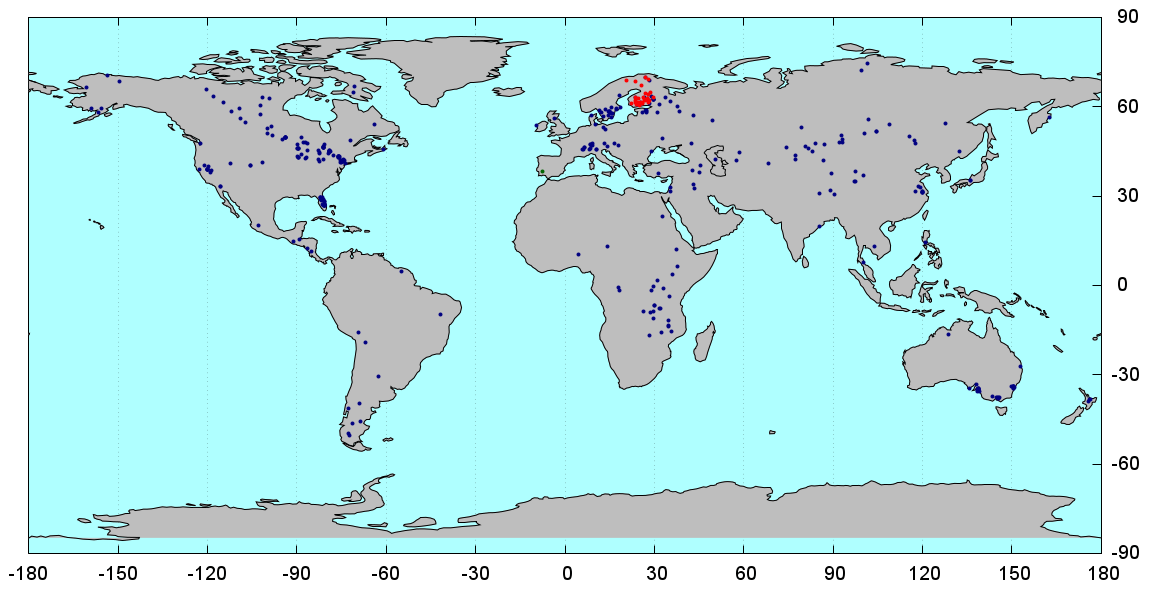
Figure 5Location of lakes with in situ data used in this study; green dots are for hourly and daily data for the Alqueva reservoir (Portugal), red for daily and 3-summer-month averaged data (Finnish lakes), blue for the 3-summer-month average data for lakes all over the globe.
3.6 River discharge
The current version of CHTESSEL does not directly produce river discharge at the river basin scale. Instead, gridded surface and subsurface runoff from CHTESSEL is coupled to the LISFLOOD hydrological and channel routing model (Van Der Knijff et al., 2010). Coupling ERA5/ERA5-Land runoff with LISFLOOD allows for lateral connectivity of grid cells with runoff routed through the river channel to produce river discharge (m3 s−1). This is the process used within the Global Flood Awareness System (GloFAS; https://www.globalfloods.eu/, last access: 29 August 2021). More details can be found in Harrigan et al. (2020). River discharge estimates from ERA5 (GloFAS-ERA5) and ERA5-Land (GloFAS-ERA5-Land) were obtained for the period January 2001 to December 2018. This is the common period for which reanalysis data were available at the time of this study. Estimates were resampled to the GloFAS 0.1∘ gridded river network at a daily time step. As part of GloFAS, a database of global hydrological observations for 2042 stations is held, consisting predominantly (i.e. ∼ 75 %) of the Global Runoff Data Centre (GRDC) and supplemented by data collected through collaboration with GloFAS partners worldwide to improve spatial coverage. The locations of the stations have been matched to the corresponding cells on the 0.1∘ GloFAS river network. Following Harrigan et al. (2020), a number of criteria were used to select stations for the evaluation:
-
at least 4 years of data available between 2001 and 2018 (not necessarily contiguous),
-
minimum upstream area of 500 km2,
-
difference in catchment area supplied by the data provider and upstream area for the corresponding cell on the GloFAS river network must be within 20 %, and
-
station with the longest record retained when multiple observation stations were matched to the same GloFAS river cell.
In addition to the above conditions, a first-order visual quality check on observed river discharge time series removed stations with erroneous data (for example, time series truncated above a threshold, showing several inhomogeneities or series monitoring an artificial canal instead of a river). This filtering procedure resulted in the selection of 1285 stations with drainage areas ranging between 575 and 4 664 200 km2, and a median of 29 963 km2. Following the methodology of Harrigan et al. (2020), hydrological performance was assessed using the modified Kling–Gupta efficiency (KGE′) metric (Gupta et al., 2009; Kling et al., 2012). The KGE′ is an overall summary measure consisting of three components important for assessing hydrological dynamics: temporal errors through correlation, bias errors, and variability errors:
where R is the Pearson correlation coefficient between reanalysis simulations (s) and observations (o), β is the bias ratio, γ is the variability ratio, μ the mean discharge, and σ the discharge standard deviation. The KGE′ and its three decomposed components (correlation, bias ratio, and variability ratio) are all dimensionless, with an optimum value of 1. To evaluate the hydrological skill of GloFAS-ERA5-Land, the KGE′ can be computed as a skill score, KGESS, with GloFAS-ERA5 used as the benchmark:
where KGE is the KGE′ value for the GloFAS-ERA5-Land reanalysis against observations, KGE is the KGE′ value for the GloFAS-ERA5 benchmark against observations, and KGE is the value of KGE′ for a perfect simulation, which is 1. KGESS=0 means the GloFAS-ERA5-Land reanalysis is no better than the GloFAS-ERA5 benchmark and thus has no skill, KGESS>0 indicates when GloFAS-ERA5-Land is considered skilful, and KGESS<0 is when the performance is worse than the GloFAS-ERA5 benchmark.
3.7 Energy fluxes
3.7.1 FLUXNET data
The evaluation of the ERA5-Land turbulent fluxes estimates was conducted mostly following the method of Martens et al. (2020). Surface sensible and latent heat fluxes (also denoted in this paper as H and λρE, respectively) derived from ERA reanalyses, as well as their ratio (i.e. the Bowen ratio, hereafter denoted as β), were compared to measurements from the FLUXNET 2015 synthesis dataset (Pastorello et al., 2020). The period under evaluation was based on the availability of reanalysis data at the time of the comparison, and therefore, unlike in Martens et al. (2020), the evaluation period is constrained to 2001–2014. Following Martens et al. (2017), the in situ flux data were subjected to quality control, including (1) the removal of rainy intervals, during which eddy-covariance measurements are typically unreliable, and (2) the removal of gap-filled records to retain only the actual measurements from the eddy-covariance sites. After quality control, only sites with a minimum record of 5 years were retained too. In total, 65 eddy-covariance sites remained after quality control and were used as in situ reference data. Note that the measured energy fluxes used as reference in this paper were not corrected for energy balance closure because the number of towers used for validation would be drastically reduced, as the ground-heat flux is also needed and is not available from many towers. Some authors have already highlighted the lack of closure in the energy balance at eddy-covariance sites and a consequential tendency to underestimate the latent heat flux (Wilson et al., 2002; Ershadi et al., 2014; Jiménez et al., 2018). The reference sites are mainly distributed across the continental US, Europe, and Australia (see their locations in Fig. 17a, b, and c, respectively). For each eddy-covariance site, the in situ measurements were aggregated from their native temporal resolution to hourly, 3-hourly, and daily intervals. In addition, standardized anomalies were calculated by subtracting for each time interval the climatological expectation (i.e. the average value across the entire record for that interval) and dividing by the standard deviation of that climatology. While the comparison to raw time series may mask the influence of short-term meteorological anomalies on surface energy partitioning (as the temporal variability of turbulent fluxes typically depends strongly on the seasonality of its main drivers), the comparison to anomaly time series reflects the response to short-term meteorological conditions. The Bowen ratio was only calculated at daily temporal resolution for numerical instability reasons. As described in Martens et al. (2020), outliers in the time series of the Bowen ratio, for both the reanalyses and in situ data, were masked using a quantile-based approach. The bias, i.e. the difference between raw in situ time series and reanalysis estimates, the standardized MAE, and the anomaly Pearson correlation coefficient (RAN) were computed. The results are shown in the form of violin plots in Sect. 4.5.1.
3.7.2 GLEAM
The Global Land Evaporation Amsterdam Model (GLEAM; Miralles et al., 2011; Martens et al., 2017) is used in this study with two objectives: (a) to compare the GLEAM evaporation estimates directly to the ERA5 and ERA5-Land estimates, which in turn will assess the skill of the underlying land surface model to simulate turbulent heat fluxes, and (b) as an intermediate tool to assess the quality differences of key input meteorological drivers of the turbulent fluxes computed by GLEAM. GLEAM is a process-based, yet semi-empirical, model that computes total evaporation and its separate components over continental masses at global scale. A detailed description of this model can be found in Martens et al. (2017) and Miralles et al. (2010, 2011). In this paper, version 3 (v3) of the GLEAM algorithm is used and forced with the same database as in the official v3.4a dataset (see https://www.gleam.eu, last access: 29 August 2021), including near-surface air temperature and surface net radiation from ERA5; this dataset is hereafter referred to as GLEAM + ERA5. Likewise, a version of GLEAM run with ERA5-Land air temperature and surface net radiation is referred to as GLEAM + ERA5-Land. Analogous comparisons between GLEAM + ERA5 and GLEAM + ERA-Interim (using forcing fields from ERA-Interim) can be found in Martens et al. (2020). Surface latent heat flux, surface sensible heat flux, and the Bowen ratio from GLEAM + ERA5 and GLEAM + ERA5-Land were evaluated against the eddy-covariance data described in Sect. 3.7.1 at daily timescales.
3.8 Skin temperature
The skin temperature is the theoretical temperature of the Earth's surface that is required to satisfy the surface energy balance. It represents the temperature of the uppermost surface layer, which has no heat capacity and thus can respond instantaneously to changes in surface fluxes. The top surface layer of the ECMWF's land surface model, CHTESSEL, covers the top 7 cm. In order to evaluate the skill of ERA5-Land land surface temperature (LST), NASA's Moderate Resolution Imaging Spectroradiometer (MODIS) MYD11C3/MOD11C3 version 6 product was used in this study. It provides monthly LST and emissivity values for Aqua and Terra in a 0.05∘ (5600 m at the Equator) latitude–longitude climate modelling grid (CMG), for day and night overpasses. Chen et al. (2017) recommended the use of the MODIS LST average ensemble (i.e. from Aqua-day, Aqua-night, Terra-day, and Terra-night) for climate studies and reported validation with 156 flux tower measurements (RMSE = 2.65, mean bias < ±1 K). In this study, the MODIS observational LST ensemble was constructed following Chen et al. (2017) and used as a reference for comparison with ERA-Interim, ERA5, and ERA5-Land monthly averaged LST data for the period January 2003 to December 2018 (16 years). MODIS data were firstly averaged to monthly timescales and then upscaled at two spatial resolutions: to 0.1∘ for comparison to ERA5-Land, and to 0.25∘ for comparison to ERA5 and ERA-Interim data. Bias, Pearson's correlation (R), and RMSE were computed on the full time series, and correlation was also computed on the anomalies (RAN), calculated as departures from the monthly climatology.
4.1 Soil moisture
Figure 6 shows the evaluation results for ERA5-Land and ERA5 top soil moisture layer against 5 cm depth measurements for sites in Europe, Africa, and Australia. For sites in Europe, both ERA5-Land and ERA5 show similar STDD and bias distributions (Fig. 6a, c). The distribution of R is also similar but the median value obtained for ERA5-Land is slightly higher than for ERA5 (Fig. 6b). In contrast, ERA5 shows a slightly higher median for the anomaly correlation, although ERA5-Land shows a more compact distribution (Fig. 6d). In Africa, only 10 sensors at a depth of 5 cm were available. The STDD shows a larger distribution for ERA5-Land (Fig. 6e); however, the latter shows slightly lower bias and better R (Fig. 6f, g). The anomaly correlation is largely improved (Fig. 6h). Finally, in Australia, ERA5-Land box plots (Fig. 6i–l) clearly show lower STDD and bias, and higher R than ERA5 (both for the original time series and the anomaly times series). The evaluation obtained over Europe, Africa, and Australia shows an overall slightly better performance of ERA5-Land over ERA5; in particular, the anomaly correlation of the top layer is improved predominantly in the warmest climates. Nonetheless, these results for the top soil layer are not conclusive, partly because of the insufficient number of available stations.

Figure 6Box plots showing the evaluation of ERA5-Land and ERA5 top layer soil moisture against in situ measurements at 5 cm for sites in Europe (a–d), Africa (e–h), and Australia (i–l). Panels (a), (e), and (i) show the standard deviation of the difference (STDD), (b), (f), and (j) the Pearson correlation coefficient (R), (c), (g), and (k) the bias, and (d), (h), and (l) the Pearson correlation of the anomaly time series (RAN). On each box, the central mark indicates the median, and the bottom and top edges of the box indicate the 25th (q25) and 75th (q75) percentiles, respectively. The whiskers extend to the most extreme data points not considered outliers.
To get more insight into the soil moisture evaluation, ERA5-Land and ERA5 were also evaluated over North America, where most of the in situ sensors are available, including several hundreds of sensors at 20 and 50 cm depths. In addition, the same evaluation was performed for ERA-Interim to address the evolution of ERA5 and ERA5-Land with respect to the previous reanalysis generation. Figure 7 shows the evaluation results for ERA5-Land, ERA5, and ERA-Interim soil moisture top three layers against measurements for sites in North America at 5 cm (Fig. 7a–d), 20 cm (Fig. 7e–h), and 50 cm depth (Fig. 7i–l). ERA5 and ERA5-Land surface soil moisture obtains quite similar results for all the metrics, although the median of the correlation and anomaly correlation are slightly better in ERA5-Land. ERA-Interim obtains lower values for these last two metrics, meaning that the land improvements in CHTESSEL compared to the old TESSEL scheme lead to better representation of the soil moisture dynamics. In deeper layers, the performance of ERA5-Land is better than that of ERA5, in particular for the third layer, for which ERA5-Land shows lower STDD (Fig. 7i) and higher correlation (Fig. 7j, l) than ERA5. It is worth mentioning that for the third soil layer of the model, ERA5 performs quite similarly to ERA-Interim, which is likely due to the initialization of the ERA5 streams with ERA-Interim soil moisture conditions.
Finally, the results were also analysed site per site taking into account the confidence interval of the Pearson correlation obtained for ERA5 and ERA5-Land versus the in situ measurements. A correlation difference is considered significant if the confidence intervals do not overlap. The Pearson correlation difference for ERA5 and ERA5-Land at 5 cm is significant for 382 sensors, of which 64 % shows higher correlation for ERA5-Land. The correlation difference at 20 cm is significant for 417 sites, of which 72 % show a higher correlation for ERA5-Land. Finally, the correlation difference at 50 cm is significant for 479 sites, of which 88 % show a higher correlation for ERA5-Land.
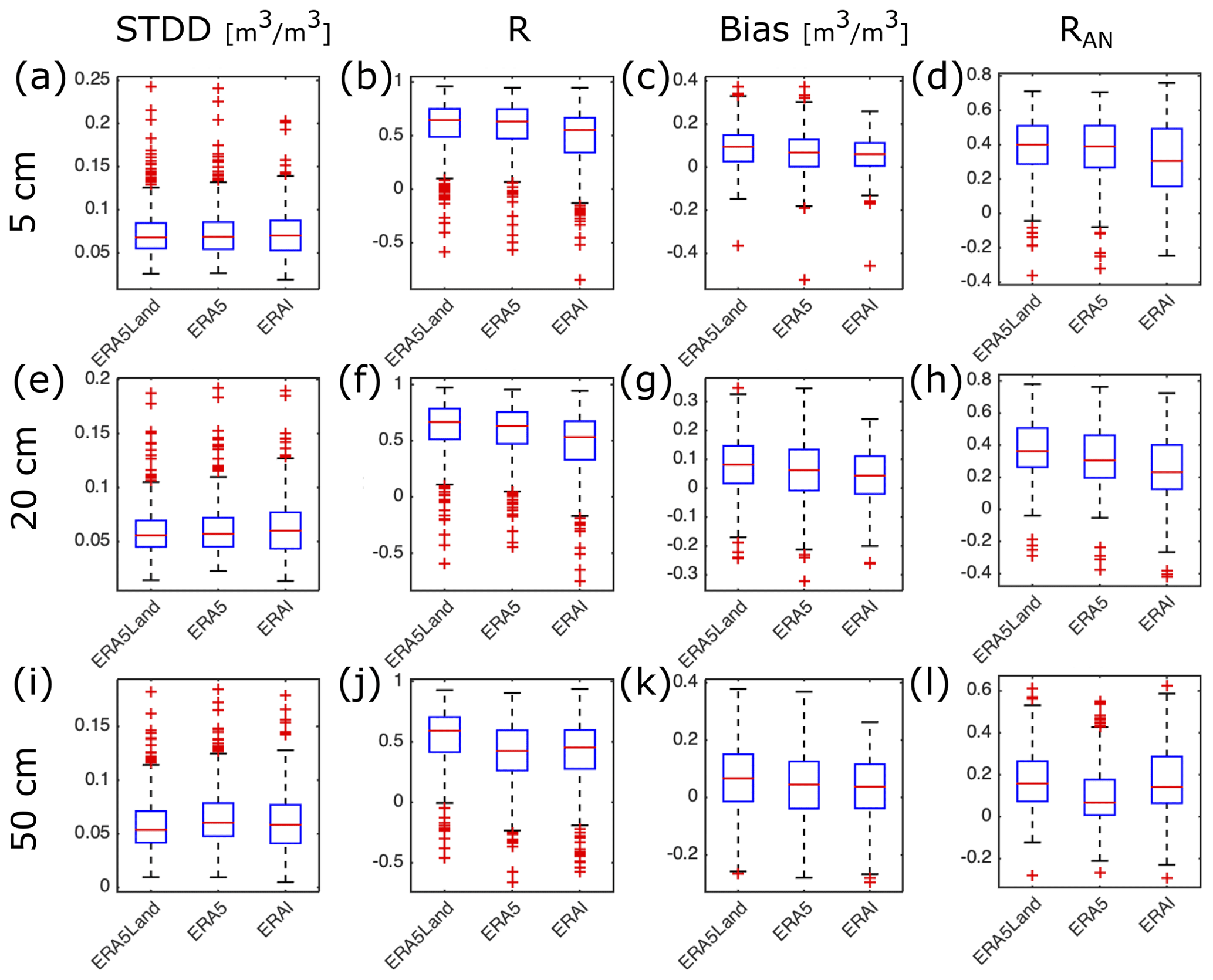
Figure 7Box plots showing the evaluation of ERA5-Land, ERA5, and ERA-Interim against in situ measurements at 5 (a–d), 20 (e–h), and 50 cm (i–l) over North America. Panels (a), (e), and (i) show the standard deviation of the difference (STDD), (b), (f), and (j) the Pearson correlation, (c), (g), and (k) the bias, and (d), (h), and (l) the Pearson correlation of the anomaly time series (RAN). On each box, the central mark indicates the median, and the bottom and top edges of the box indicate the 25th (q25) and 75th (q75) percentiles, respectively. The whiskers extend to the most extreme data points not considered outliers.
4.2 Snow
Figure 8 shows the mean bias and RMSE of the SWE normalized by the mean value and standard deviation of the observations, respectively, for the 10 sites of Table 3. Each column displays the statistics of the nearest neighbour point, whereas the vertical bars represent the minimum and maximum values of the metrics computed over the four nearest points. Hence, this enables the characterization of the spatial variability of the errors given that many sites are located in complex terrains or coastal area.

Figure 8Summary statistics of the normalized mean bias (a) and RMSE (b) of snow water equivalent (SWE) at each ESM-SnowMIP site for ERA5-Land (red), ERA5 (green), and ERA-Interim (cyan). ESM-SnowMIP sites are described in Table 3. Each reanalysis box has a vertical line representing the variability at the four nearest grid points to the site location.
Considering the mountain sites, ERA5-Land shows lower RMSE over the sites with moderate altitude, i.e. between 1300 and 2500 m (cdp, rme, wfj). ERA5-Land also clearly presents the lowest errors in the Arctic site (sod) and in the boreal forest sites (oas, obs, and ojp). Overall, the biases are smaller in ERA5-Land than in ERA5 (and ERA-Interim) at these sites. For the mountain sites, all reanalyses are characterized by a negative bias, which is very likely due to the smoothing of the orography at the resolution of the reanalysis. The higher horizontal resolution of ERA5-Land, compared to ERA5, helps to reduce the bias at cdp, rme, and wfj caused by a better orographic representation. However, the agreement with in situ observations at the sites located in very high mountains (snb and swa, located at altitudes greater than 3300 m) is slightly better with ERA5 than with ERA5-Land. It should be noted that the four nearest grid points indicate a much larger spread of errors for ERA5 than for ERA5-Land. Therefore, compensating errors could lead to better performance of ERA5 at the nearest grid point. The maritime site (sap) also shows lower RMSE in ERA5. At this site, the data assimilation can help in adding/removing snow mass for the right reason (snow density is overall well represented at this site; see time series in Fig. S1 in the Supplement), even though the spatial variability is higher in ERA5. On the contrary, at the forest sites (oas, obs, ojp), snow depth assimilation can remove snow mass to compensate for errors in snow density, the latter which are not considered in the assimilation system. Finally, noteworthy are the improvements in the transition between ERA-Interim and ERA5, in particular at Sodankylä (sod), which is caused by improved parameterizations of the snow model introduced between ERA-Interim and ERA5 productions (Dutra et al., 2010).
Figure 9 shows the maps of the RMSE difference between ERA5-Land and ERA5 snow depth estimates when compared to in situ observations of the GHCN network, for both North America and Europe. Over the US, and particularly over the Rockies region, ERA5-Land generally outperforms ERA5 in terms of lower RMSE (see Fig. 9a). In these highly complex terrain regions, the higher horizontal resolution of ERA5-Land adds value by providing more realistic orographic contours. However, over Europe (i.e. mainly Scandinavia; see Fig. 9b), where ERA5 uses a dense SYNOP network of observations in the snow assimilation system, ERA5 performs better than ERA5-Land.

Figure 9Snow depth RMSE difference between ERA5-Land and ERA5 (with respect to GHCN observations) for the months of December to June between 2010 and 2018. Negative values indicate better matching of ERA5-Land averaged snow depth with in situ measurements of the GHCN network; positive values indicate that ERA5 averaged snow depth estimates are matching better in situ measurements.
To further quantify the impact of the higher horizontal resolution of ERA5-Land on snow depth simulation, Fig. 10 shows the RMSE as a function of the height of each station. The stations were binned in height ranges of 250 m (0–250, 250–500, etc.) and the distribution of the RMSE is displayed for each height range using box plots. For heights below ≈ 1500 m a.s.l., ERA5 performs slightly better than ERA5-Land, while for heights between ≈ 1500 m a.s.l. and ≈ 3000 m a.s.l. ERA5-Land outperforms ERA5, as a result of the better resolution. For stations above 3300 m a.s.l., ERA5 performs better, which can be due to compensating errors, similarly to the ESM-SnowMIP sites. In addition, it should be noted that the number of sites at these very high altitudes is small, and therefore the statistical results should be interpreted with caution.

Figure 10Box plot of the snow depth RMSE distribution as function of the site altitude, for North America (30–80∘ N, 60–160∘ W, a) and Europe (25–80∘ N, 10∘ W–40∘ E, b), for ERA5-Land (red), ERA5 (green), and ERA-Interim (cyan). Boxes extend between the lower (25 %) and upper quartiles (75 %), and the horizontal lines within each box represent the median value of the distribution. The black line represents the number of stations grouped at each bin.
4.3 Lakes
The ERA5 and ERA5-Land hourly estimates of LSWT compared to the hourly data of the Alqueva reservoir showed that ERA5-Land obtained statistically significant MAE reduction by 2.2 % (see Table 4). While this is a positive result, ERA5-Land data showed some rapid changes in the lake mixed-layer depth (up to 5 m), which led to a quick rise of the lake surface water temperature (up to 20 ∘C). The left plot of Fig. 11 shows the bias distribution for hourly data; even though the frequency of bias around zero is larger for ERA5-Land (indicating more accurate estimates of LSWT), errors due to unrealistic temperature rise are also visible at higher frequency between 3–4 ∘C.
Table 4MAEs of the ERA5 and ERA5-Land LSWT estimates compared to in situ hourly, daily, and 3-summer-month average LSWT data. Hourly data correspond to data from the Alqueva reservoir in Portugal (2017 and 2018); daily data are from the Finnish lakes (2000–2016) and averaged hourly data from the Alqueva reservoir; summer month average data are from a global inventory (1985–2009) and the Finnish lakes. The first column is for the data type (hourly/daily/summer month average), second column provides the number of lakes for each category, third column shows the MAE (∘C) of ERA5 LSWT estimates compared to in situ measurements, and fourth column is the same as third column but for ERA5-Land.
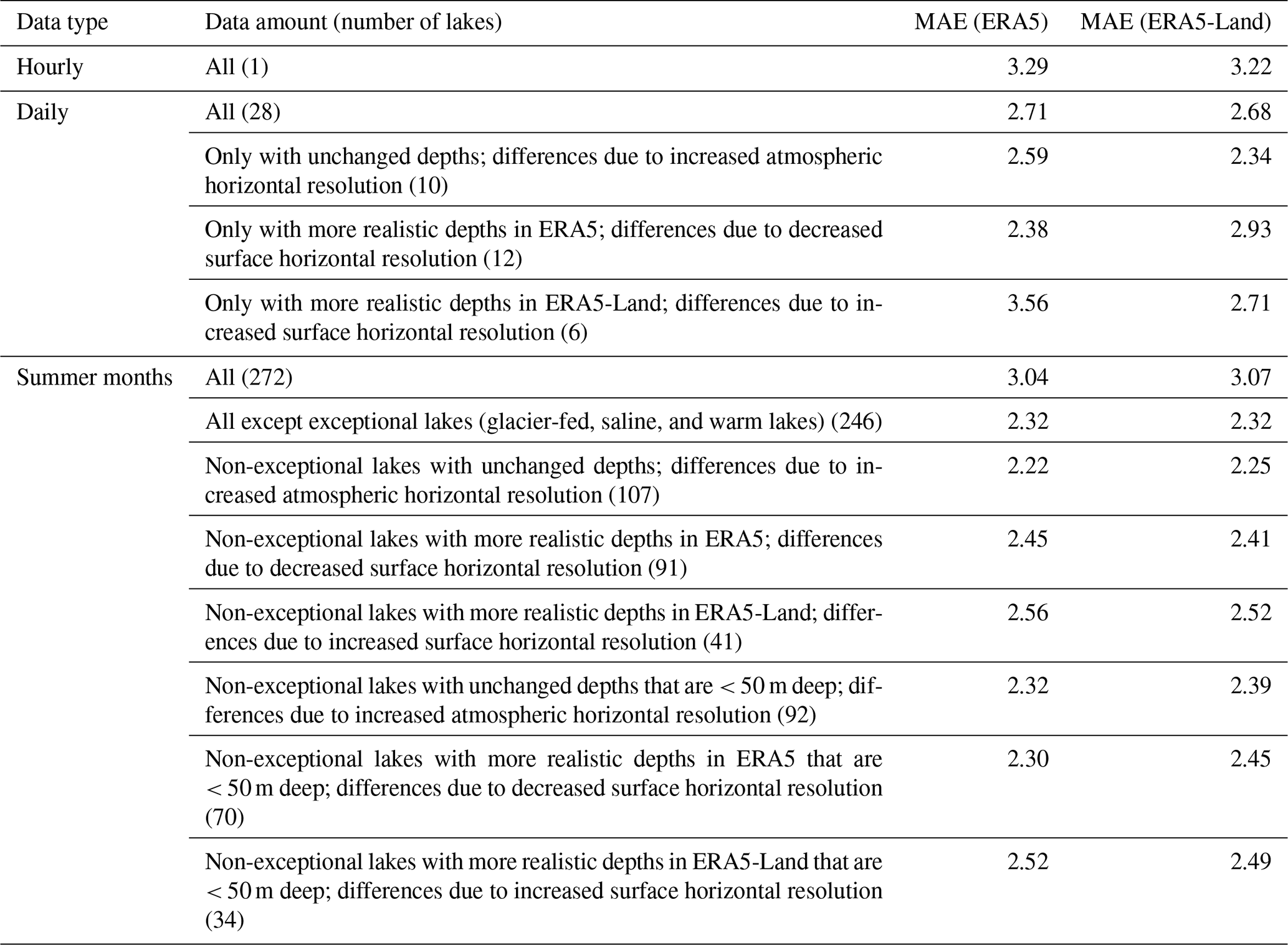
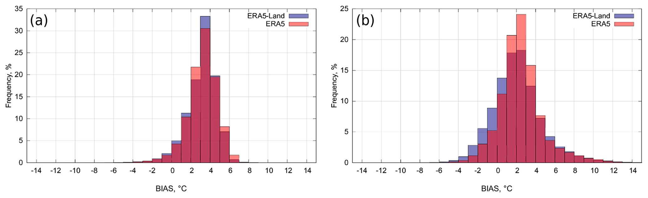
Figure 11LSWT bias (observations minus ERA5 or ERA5-Land estimates) distribution (∘C) for hourly data from the Alqueva reservoir (a) and daily data from the Alqueva reservoir and the Finnish lakes (b). The dark red colour represents the area where both ERA5 (pink colour) and ERA5-Land (violet colour) bias distribution overlap.
The comparison of the ERA5 and ERA5-Land daily averaged LSWT with Alqueva reservoir and the 27 Finnish lakes data also showed statistically significant reduction of ERA5-Land MAE (among 28 lakes) by 1.2 % (from 2.71 to 2.68 ∘C; see Table 4). It should be noted that the lake parametrization scheme relies heavily on the lake depth input data. With the increase of resolution in ERA5-Land, lake depth values change as well. For only those lakes whose depth became more realistic in ERA5-Land as result of the higher resolution, the MAE was statistically significantly reduced by 23.8 %; however, for only those lakes whose depth remained unchanged despite the change of resolution, the MAE was still statistically significantly reduced by 9.6 %, showing the positive influence of higher-resolution atmospheric input. The right plot of Fig. 11 shows, for daily data, a reduced amount of large positive errors (cold bias) in ERA5-Land and a larger frequency of errors around zero bias. Finally, only 272 lakes with averaged in situ measurements for the summer months, with 10- to 15-year data records, could be used for comparison with ERA5 and ERA5-Land LSWT estimates. The comparison showed statistically significant MAE increase by 1.0 % for ERA5-Land compared to ERA5 (see Table 4). If one bears in mind that FLake was not designed for saline, fed by glaciers or mountains and warm lakes (that excludes 26 exceptional lakes) the MAE of the remaining 246 lakes is similar in ERA5 and ERA5-Land. The right plot of Fig. 12 shows the geographical distribution of the 26 exceptional lakes and their averaged ERA5-Land MAE, which shows large LSWT errors, even beyond 10 ∘C. Note that errors for these lakes are very similar for ERA5. If, as a result of the higher resolution, only lakes whose depth became more realistic in ERA5-Land compared to ERA5 are taken into account, the MAE is statistically significantly reduced by 1.4 % in ERA5-Land. FLake was specially designed for medium depth (under 50 m) lakes. Several lakes from this database are however very deep. Nevertheless, computing the statistics for only medium depth lakes did not show any extra improvement in ERA5-Land data. The left plot of Fig. 12 presents the bias distribution of non-exceptional lakes (246) that shows wider error distribution for both ERA5 and ERA5-Land compared to hourly and daily distributions.
Figure 12LSWT bias (observations minus ERA5 or ERA5-Land estimates) distribution (∘C) for the 3-summer-month average data based on non-exceptional lakes (a), and geographical distribution of the 26 exceptional lakes (glacier-fed, saline, and warm lakes) ERA5-Land MAE (b) with colour bar in ∘C.
4.4 River discharge
Results of river discharge performance for GloFAS forced with ERA5 and ERA5-Land are shown in Fig. 13. The overall global median KGE′ across 1285 observation stations improves from 0.26 (with an interquartile range of −0.04 to 0.49) for GloFAS-ERA5 to 0.37 (0.08, 0.57) for GloFAS-ERA5-Land (Fig. 13a). In the decomposition of the KGE′, the global median Pearson correlation also improves from 0.60 (0.43, 0.75) to 0.64 (0.49, 0.77) (Fig. 13b), and global median bias ratio improves from 0.73 (0.50, 1.13) to 0.89 (0.66, 1.15) (Fig. 13c), which is equivalent to a 16 % reduction in overall bias. There is very little difference in variability errors between GloFAS-ERA5 and GloFAS-ERA5-Land (Fig. 13d).
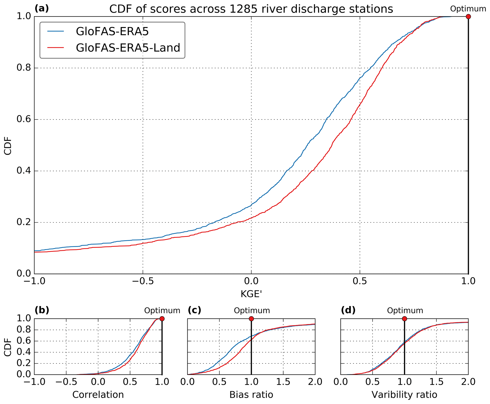
Figure 13Cumulative distribution functions (CDFs) of hydrological performance metrics across 1285 observation stations. Modified Kling–Gupta efficiency (KGE′) (a) with decomposition of KGE′ into Pearson correlation (b), bias ratio (c), and variability ratio (d) for GloFAS-ERA5-Land (red line) and GloFAS-ERA5 (blue line). The red dot marks the optimum value for each metric.
Figure 14 shows the spatial distribution of river discharge skill, measured by the KGESS. GloFAS-ERA5-Land shows positive skill compared to the GloFAS-ERA5 benchmark in 65 % of stations with a global median KGESS of 0.08 (−0.06, 0.25). Largest improvements in skill are found in North America, Europe, northern Russia, southern Africa, and Australian catchments. There is a substantial decrease in skill (i.e. KGESS < −0.2) when forcing GloFAS with ERA5-Land runoff instead of ERA5 in 11 % of stations, mainly located in the western US and South America. Care must be taken in spatial representativeness of these results, as the observation network is sparse in some regions of the world, particularly in large parts of Africa and Asia.
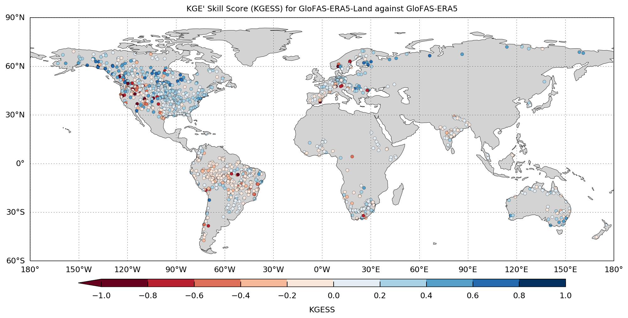
Figure 14Modified KGESS for GloFAS-ERA5-Land river discharge reanalysis against the GloFAS-ERA5 benchmark across 1285 observation stations. Optimum value of KGESS is 1. Blue (red) dots show catchments with positive (negative) skill.
4.5 Energy fluxes
4.5.1 Evaluation against eddy-covariance sites
The left panel of Fig. 15 shows the violin plots of the ERA-Interim and ERA5-Land turbulent fluxes (compared to in situ eddy-covariance measurements).
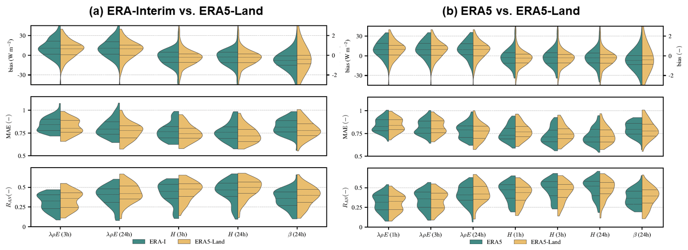
Figure 15Violin plots showing the temporally and spatially averaged statistics of the surface latent heat flux (λρE), surface sensible heat flux (H), and Bowen ratio (β) from (a) ERA-Interim (green) and ERA5-Land (yellow) and (b) ERA5 (green) and ERA5-Land (yellow). Statistics are calculated with respect to in situ eddy-covariance measurements at both 3-hourly and daily (24 h) temporal resolutions. Violin plots represent the distribution of the individual validation statistics with indication of the median and interquartile range, and are calculated using a kernel density estimation approach. Statistics include the bias, standardized MAE, and anomaly correlation coefficient (RAN). The scale used to show the bias distribution of β is that of the right y axis at the top row of each panel.
ERA5-Land compares systematically better to in situ measurements than ERA-Interim, with higher RAN values for the heat fluxes and the Bowen ratio and for both subdaily and daily temporal resolutions, as well as presenting lower bias and MAE. This result is expected, as the land surface model used in ERA5-Land benefits from many improvements compared to that of ERA-Interim (see Sect. 2.4). The right panel of Fig. 15 shows the same plot but comparing ERA5 and ERA5-Land. The violin plots are much more similar, biases for both fluxes are only marginally better in ERA5-Land (the median of the distribution is nearly the same, but the 75 % percentile is always lower), and MAE is typically lower for λρE in ERA5-Land (except at 1-hourly resolution) but higher for H. On average, correlations for ERA5-Land are only better for λρE at daily resolution and for the Bowen ratio. It also should be noted that all statistics are on average better for H than for λρE, both in ERA5 and in ERA5-Land (with lower bias, lower MAE, and higher RAN); this matches the results reported by Balsamo et al. (2015) and Martens et al. (2020). To investigate potential areas of significant improvement/degradation, the left panel of Fig. 16 shows the maps of RAN differences of λρE between ERA5-Land and ERA5, over the continental United States (CONUS). RAN is typically better for ERA5-Land across most US stations, especially near the coasts and around the lakes, where high resolution is more important. In Europe (Fig. 16, middle panel), results are very mixed, but for most of the stations in the Alps ERA5-Land performs worse than ERA5. Although for Australia ERA5-Land is slightly better than ERA5 (see right panel of Fig. 16), it is not the case for all stations. The results for the Bowen ratio are aligned with those of λρE (see Fig. S3), whereas those of H are more favourable for ERA5 (see Fig. S2).
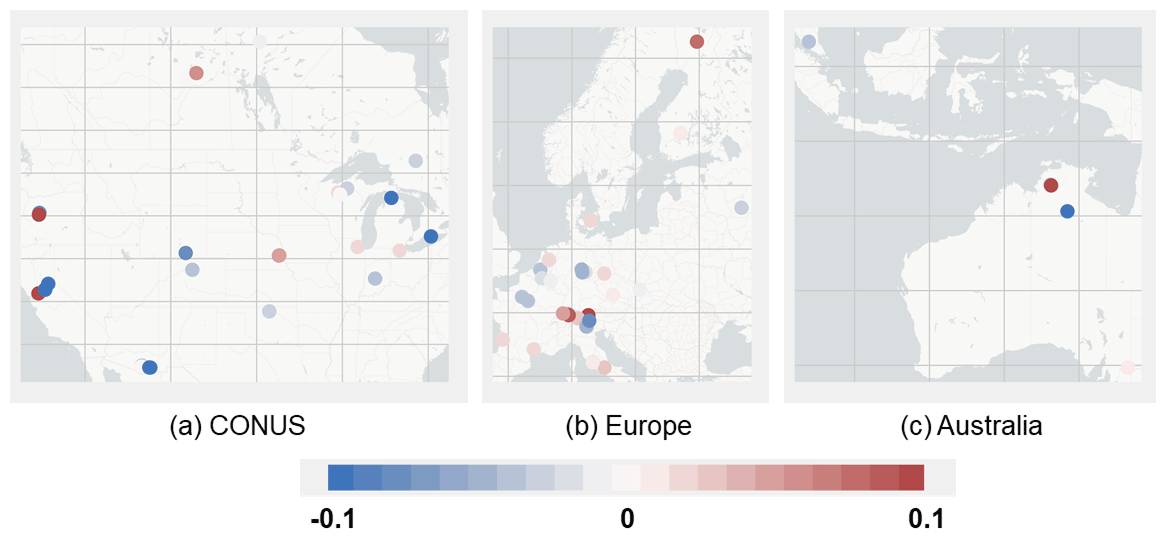
Figure 16Standardized anomaly correlation (RAN) difference of the surface latent heat flux between ERA5-Land and ERA5 with respect to eddy-covariance data. Blue colours indicate that the anomaly correlation of ERA5-Land with respect to eddy-covariance measurements is higher than for ERA5, whereas red colours indicate the opposite.
To study the influence of the eddy-covariance sites' altitude and air temperature in the heat fluxes, Fig. 17 shows the standardized mean RAN (circles) and MAE (squares) of H and λρE as a function of the station altitudes and air temperature. The results are in line with those presented in the violin plots. ERA5-Land clearly performs better for λρE and the Bowen ratio, and the largest differences between ERA5 and ERA5-Land are obtained for the sites located at high altitudes, where more extreme values are obtained and forcing errors are increased. Although for H the differences are smaller, ERA5 performs overall better than ERA5-Land and the strongest differences are also seen at high-altitude sites.
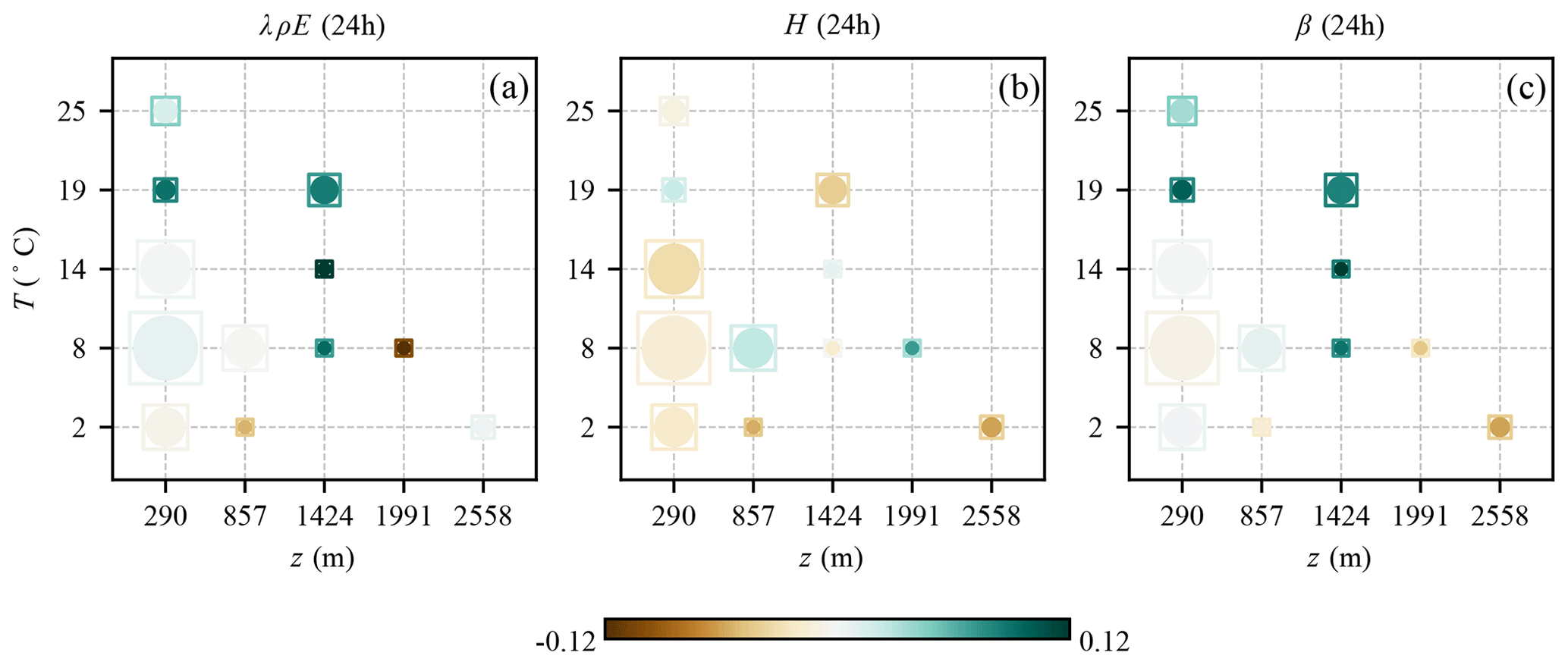
Figure 17Standardized anomaly correlation difference (circles) and standardized mean absolute differences (squares) between ERA5-Land and ERA5 latent heat flux (a), sensible heat flux (b), and Bowen ratio (c), grouped as a function of stations temperature and altitude. The size of circles and squares is proportional to the number of eddy-covariance towers. Green values denote better matching of ERA5-Land with in situ data.
4.5.2 Evaluation using GLEAM
The turbulent fluxes estimated from GLEAM forced with temperature and surface net radiation from ERA5 and ERA5-Land were also computed. ERA5-Land surface fluxes perform better than GLEAM + ERA5-Land when confronted to in situ measurements (see the violin plots in Fig. S4), except in terms of bias, in agreement with Martens et al. (2020). This result reflects the quality of the CHTESSEL land surface model, which has greatly improved the parametrization of turbulent energy fluxes and evidences the added value compared to a simpler model as in GLEAM, designed to consider only input variables that can be observed from satellite. Figure 18 is similar to Fig. 17 but comparing ERA5-Land and GLEAM + ERA5-Land, as a function of elevation and air temperature, at daily resolution. As expected, almost for all stations temperature and elevation, ERA5-Land heat fluxes match better the in situ reference measurements. The exceptions are towers at the highest altitudes where forcing errors are generally larger. Comparing GLEAM + ERA5 and GLEAM + ERA5-Land, the differences are very small, suggesting that the near-surface air temperature and net radiation are quite similar in both reanalyses for the locations of the eddy-covariance sites.
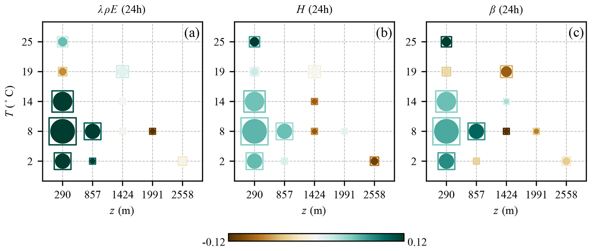
Figure 18Standardized anomaly correlation difference (circles) and standardized mean absolute differences (squares) between ERA5-Land and GLEAM + ERA5-Land latent heat flux (a), sensible heat flux (b), and Bowen ratio (c), grouped as a function of stations' temperature and altitude. The size of circles and squares is proportional to the number of eddy-covariance towers. Green values denote better matching of ERA5-Land with in situ data.
4.6 Skin temperature
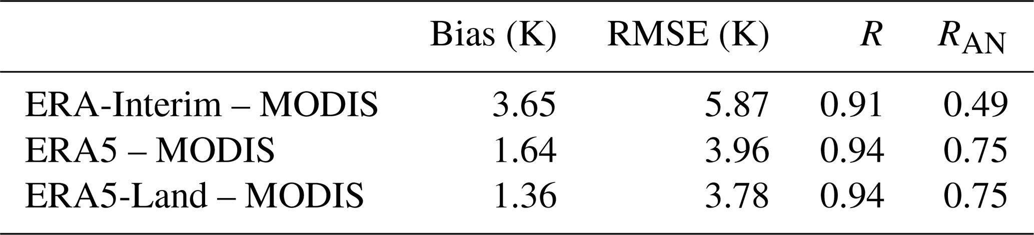
Figure 19 shows global maps of ERA5-Land and ERA-Interim mean LST for the time period 2003–2018, as well as global maps of their correlation and RMSE with respect to the MODIS LST average ensemble, constructed as indicated in Sect. 3.8. While differences in mean LST are apparently minimal among the two simulated products, there is a better correlation of ERA5-Land with MODIS in the tropical band. The low correlation obtained between the simulated and the remotely sensed LST over tropical forests should be taken with caution since persistent cloud cover as well as cloud contamination effects are known to have an impact on remotely sensed observations, leading to important differences in their absolute values (Jiménez-Muñoz et al., 2016; Gomis-Cebolla et al., 2018). Notably, ERA5-Land systematically compares better than ERA-Interim to MODIS LST in terms of RMSE, particularly at high latitudes. As shown in the averaged statistical scores on Table 5, there is an overall improvement of ERA5 and ERA5-Land LST simulations with respect to ERA-Interim, yet only modest improvements are achieved in ERA5-Land compared to ERA5 LST, mainly on bias and RMSE. The better correlation of MODIS with ERA5 and ERA5-Land than with ERA-Interim is more evident in RAN maps (see Table 5 and Fig. S5).
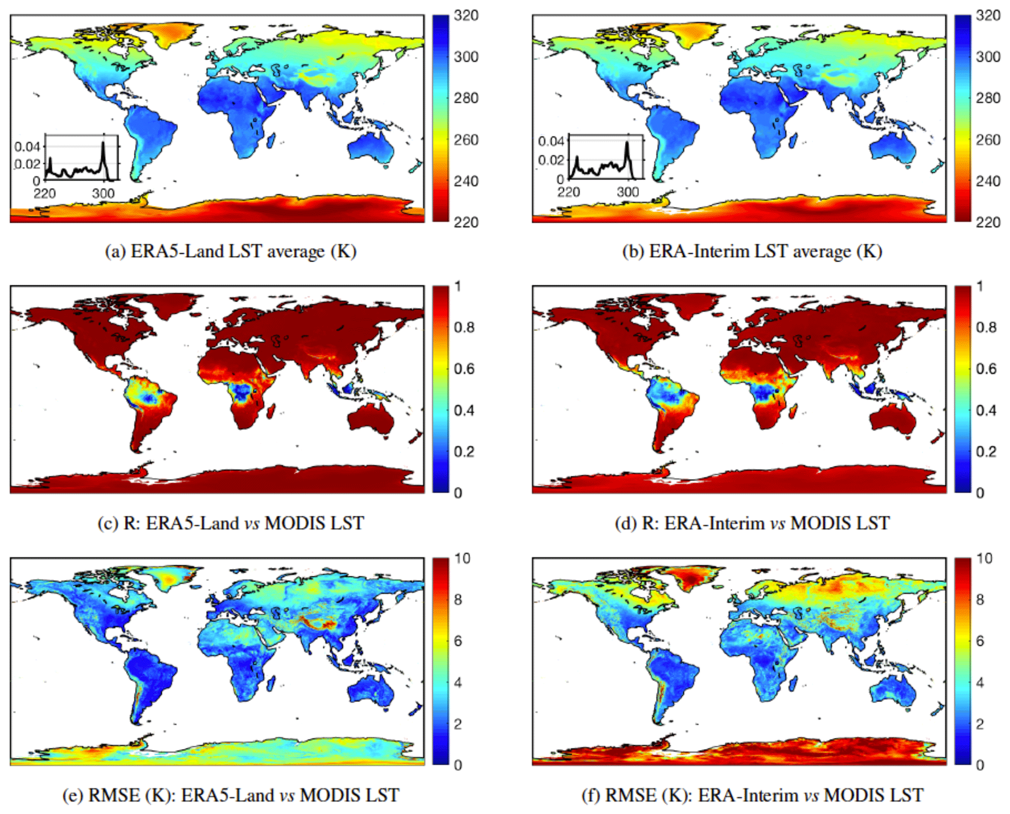
Figure 19Global statistics of ERA5-Land (a, c, e) and ERA-Interim (b, d, f) LST (in K) for the time period 2003–2018. Panels (a) and (b) are the global maps of mean LST, (c) and (d) are the correlation maps, and (e) and (f) are the RMSE maps, with respect to the MODIS LST average ensemble. Note that the LST here refers to the skin temperature.
To further scrutinize the impact of the ERA5-Land higher horizontal resolution on LST simulation, ERA5 LST was resampled to 0.1∘ and then global maps of the RMSE difference (ΔRMSE) between ERA5 and ERA5-Land with respect to the MODIS LST average ensemble were calculated. The improvement of ERA5-Land on LST in coastal areas is clearly visible in the ΔRMSE maps, as shown in Fig. 20 for the European domain. The time series at the coastal pixel in Norway illustrates how ERA5-Land LST simulations compare better to the observational record by capturing more closely the annual cycle in its whole range of variability, and therefore decreasing bias and RMSE, while the correlation with the MODIS product is very good and almost similar for both reanalyses. The time series at the other two specific locations illustrate regions of complex topography exhibiting slightly lower RMSE of ERA5-Land (Iceland), and of ERA5 (Alps), with respect to the MODIS LST average ensemble. These results highlight improved LST simulations of ERA5-Land on coastal regions.
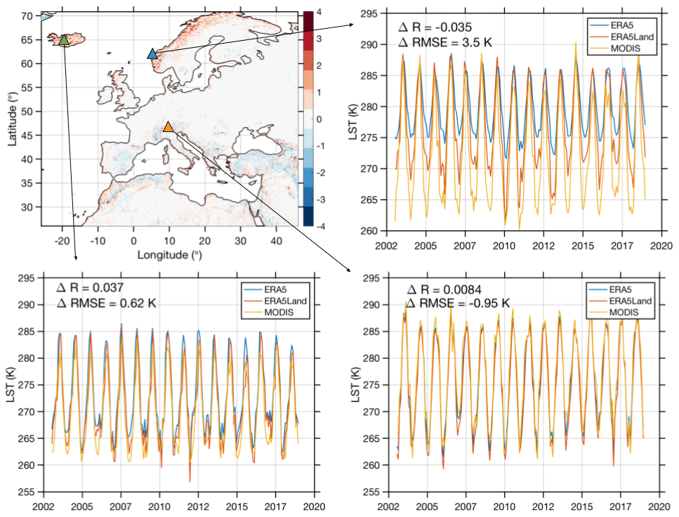
Figure 20Map of RMSE differences (ΔRMSE (K)) between ERA5 and ERA5-Land with respect to the MODIS LST average ensemble for the time period 2003–2018. Red values denote lower RMSE of ERA5-Land with respect to the observational record. Time series of ERA5, ERA5-Land, and MODIS time series at selected pixels: coast of Norway (61.6∘ N, 5.3∘ E), the Alps (47.4∘ N, 11.15∘ E), and Iceland (64.5∘ N, 20.26∘ W). The differences in RMSE (ΔRMSE) and R (ΔR) between ERA5 and ERA5-Land with respect to MODIS LST at each location are reported.
Table 5Spatially and temporally averaged bias, RMSE, R, and anomaly correlation coefficient (RAN) between ERA-Interim, ERA5, and ERA5-Land estimates and the MODIS land surface temperature average ensemble for the time period 2003–2018.
ERA5-Land data are available through the C3S CDS, and at the time of writing this paper the data are available from January 1981. The data are accessible either via the user interface (https://cds.climate.copernicus.eu/cdsapp#!/dataset/reanalysis-era5-land?tab=overview, last access: 29 August 2021, Muñoz-Sabater, 2019a) or through the CDS application program interface (API). The data are updated with 2–3 months' delay with respect to real time. However, a close-to-real-time facility is planned to be implemented in 2021. The atmospheric forcing used to drive the land simulations is also available and already interpolated to the ERA5-Land grid. Note that in the CDS, and for user convenience, the data have been interpolated to a regular lat–long grid of 0.1∘ resolution.
All ERA5-Land fields are made available at hourly temporal resolution and post-processed as monthly means. Monthly means are easier to handle and faster to retrieve, which is especially well suited for climate studies and also addresses an important requirement of reanalysis users. Two types of monthly means are post-processed:
-
monthly means of daily means (average over all the hourly fields in a month):
-
monthly means of synoptic means (averaged for a specific time of the day in a month):
with 〈x〉 the estimate of the monthly average for the field x, Nd the number of days in a month, Ns the number of forecast steps in a day, ℳ the forecast model, d the day, and s the forecast step from 00:00 UTC in a 24 h cycle. Note that the water and energy fluxes are accumulated from the beginning of the forecast time at 00:00 UTC with a maximum of 24 h accumulation period. For example, the monthly mean of surface runoff at 12:00 UTC will provide the monthly averaged runoff accumulated from 00:00 to 12:00 UTC. Therefore, for water and energy fluxes, Eq. (6) becomes
-
monthly means of daily means for water and energy fluxes
Further technical details are also provided in the online documentation (https://confluence.ecmwf.int/display/CKB/ERA5-Land:+data+documentation, last access: 31 August 2021).
ERA-Interim surface data used in this study are freely available through the ECMWF catalogue: https://apps.ecmwf.int/datasets/data/interim-full-daily/levtype=sfc/ (Dee et al., 2011).
ERA5 hourly data on single levels used in this study are also freely available through the C3S CDS (https://doi.org/10.24381/cds.adbb2d47, Hersbach et al., 2018).
All soil moisture data used for validation are available through the International Soil Moisture Network, https://ismn.earth (last access: 29 August 2021, Dorigo et al., 2011, 2021).
Access to the lake data used for evaluation in this paper is provided as follows:
-
The Alqueva reservoir hourly data were provided by the Portuguese University of Évora, data are provided on demand (personal communication with Miguel Potes, Maksim Iakunin, and Rui Salgado).
-
The 27 Finnish lakes' daily data provided by Finnish Environment Institute (SYKE) are open access and available at http://rajapinnat.ymparisto.fi/api/Hydrologiarajapinta/1.0/ (SYKE, 2017).
-
Summer month (June, July, and August) averaged values from the global inventory “Globally distributed lake surface water temperatures collected in situ and by satellites; 1985–2009” are freely available at https://doi.org/10.6073/pasta/379a6cebee50119df2575c469aba19c5 (Sharma et al., 2014).
The ESM-SnowMIP dataset used for the evaluation of the snow fields is available at https://doi.org/10.1594/PANGAEA.897575 (Ménard and Essery, 2019; see also Ménard et al., 2019). The snow depth dataset from the GHCN-daily network is available at https://www.ncdc.noaa.gov/ghcnd-data-access; the version used is v3.24 (Menne et al., 2012b).
The majority (i.e. 75 %) of river discharge observation stations used in the evaluation are openly available from GRDC: https://www.bafg.de/GRDC/EN/Home/homepage_node.html (last access: 29 August 2021). The remaining stations have been shared by GloFAS partners worldwide to improve spatial coverage. The benchmark river discharge reanalysis dataset, GloFAS-ERA5 (version 2.1), is openly available from the CDS: https://cds.climate.copernicus.eu/cdsapp#!/dataset/cems-glofas-historical?tab=overview (last access: 29 August 2021) with https://doi.org/10.24381/cds.a4fdd6b9 (Harrigan et al., 2019).
GLEAM data were accessed from https://www.gleam.eu/ (last access: 29 August 2021, Martens et al., 2017; Miralles et al., 2011), and the FLUXNET2015 Tier2 dataset can be accessed from the FLUXNET data portal at https://fluxnet.org/data/fluxnet2015-dataset (last access: 29 August 2021, Pastorello et al., 2020). This work used eddy-covariance data acquired and shared by the FLUXNET community, including these networks: AmeriFlux, AfriFlux, AsiaFlux, CarboAfrica, CarboEuropeIP, CarboItaly, CarboMont, ChinaFlux, Fluxnet-Canada, GreenGrass, ICOS, KoFlux, LBA, NECC, OzFlux-TERN, TCOS-Siberia, and USCCC. The FLUXNET eddy-covariance data processing and harmonization was carried out by the ICOS Ecosystem Thematic Center, AmeriFlux Management Project, and Fluxdata project of FLUXNET, with the support of CDIAC, and the OzFlux, ChinaFlux, and AsiaFlux offices.
MODIS LST data from Aqua and Terra (https://doi.org/10.5067/MODIS/MOD11C3.006, Wan et al., 2015) platforms are available through the Land Processes Distributed Active Archive Center (https://lpdaac.usgs.gov/, last access: 27 August 2021).
FLUXNET-2015 data used for the evaluation of GPP, NEE, and Reco are available from the Drought-2018 ecosystem eddy-covariance flux product in FLUXNET-Archive format – release 2019-1 (version 1.0); ICOS Carbon Portal, https://doi.org/10.18160/PZDK-EF78 (ICOS-ETC Drought 2018 Team, 2019).
This paper presents the new global ERA5-Land reanalysis. When the historical part is completed, it will provide a detailed record of the land surface evolution from 1950 to the present through a series of key land surface variables representing the water and energy cycles. The temporal resolution is hourly and the horizontal resolution is 9 km, making it unique and suitable for a growing number of land surface applications. The quality of ERA5-Land fields was evaluated by direct comparison to a large number of in situ observations collected mainly for the period 2001–2018, as well as by comparison to additional model or satellite-based global reference datasets. The evolution of the operational ERA series of reanalyses was also assessed by adding ERA-Interim and ERA5 global reanalyses to the evaluation exercise. Key components of the water and energy cycles were analysed. Overall, the water cycle is improved in ERA5-Land compared to ERA5 according to the different variables evaluated, whereas the energy cycle variables show similar performance; both ERA5 and ERA5-Land perform substantially better than ERA-Interim. The main evaluation findings are as follows:
- a.
Soil moisture: the box plots show a consistent improvement of the statistical metric distributions of ERA5-Land with respect to those of ERA5, in particular the improvement is more marked for the root-zone soil moisture. The root zone is characterized by a slow temporal variation and thus a good initialization is crucial to reach equilibrium on relatively short timescales. ERA5 root-zone soil moisture is penalized by initialization from ERA-Interim, which leads to a multi-annual artificial trend of the time series over arid to semi-arid climates, where the standard deviation of soil moisture is low. On the contrary, the shallow surface layer responds quickly to short-term meteorological forcing variables, and hence, for the top layer, ERA5-Land only improves slightly on ERA5 estimates at the reference stations. The main added value of high resolution at the top layer is to account for the correct soil type that changes the saturation level and the minimum level at which evapotranspiration no longer occurs. Consequently, ERA-Interim, with coarser resolution, shows the lowest performance of the three reanalyses datasets. Supporting these findings, ERA5-Land participated in a soil moisture intercomparison of 18 products against large number (826) of in situ stations and performed strongly (Beck et al., 2021).
- b.
Snow: ERA5-Land snow mass and snow depth estimates are improved on mid-altitude mountains, where the higher resolution provides better orographic contours and the temperature correction is also important. However, ERA5 snow depth estimates match measurements slightly better at the highest mountains (> 3300 m). At these altitudes, uncertainties in both the forcing and in the model parametrization are larger and can contribute to the growth of errors; processes like snow transport and sublimation, which are not considered in the current snow scheme formulation, can be important at these altitudes, as well as errors in the amount of solid precipitation. It is also worth noting that for high-altitude stations, the spread of errors is larger in ERA5 compared to ERA5-Land, which could lead to error compensation. The results per continent show the best performance of ERA5-Land snow fields in the US, especially in complex orographic areas, where spatial resolution is foremost. It implies a more accurate near-surface air temperature, especially over mountains, which leads to a better representation of the sensible heat flux and therefore better estimates of the snow depth. Also, there is a limited number of snow depth in situ observations assimilated in ERA5 over the US (de Rosnay et al., 2015), and therefore the assimilation system hardly compensates for systematic model/snowfall biases. Contrarily, ERA5 performs better over Scandinavian countries. In general, snowfall in the IFS suffers from a systematic positive bias (snow overestimation) in Europe. Although data assimilation is intended to correct for random errors, snow depth reports assimilated in ERA5 alleviate the systematic snow excess where these reports are assimilated. The improvement of the snow scheme over the previous decade is also reflected in the overall better scores of ERA5 compared to ERA-Interim.
- c.
Lakes: LSWT is slightly improved in ERA5-Land at hourly and daily averaged steps with respect to in situ data at sites in Portugal and Finland. Note however that at punctual times of the warm period in Alqueva, sudden jumps of the ERA5-Land mixed-layer depth lead to unrealistic LSWT. For instance, on 3 August 2018, from 08:00 to 09:00 LT, the mixed-layer depth jumped 5.3 m, leading to a 17.6 ∘C increase and increasing the Alqueva reservoir LSWT to 40.7 ∘C. Jumps are caused by a simplistic parametrization of the summer stratification in the lake scheme, as temperature is computed differently in calm and turbulent conditions. Ways to limit these jumps and to enable a smoother and more realistic transition are currently being investigated at ECMWF. The lake parametrization scheme relies heavily on accurate lake depth input data, and therefore poor data impact its ability to accurately simulate lake parameters such as LSWT. The higher resolution of ERA5-Land allows, in many cases, a more accurate specification of lake depth. Thus, isolating lakes whose depth is more realistic using the ERA5-Land grid (i.e. only lakes whose depth in the ERA5-Land grid matches better in situ observations), the LSWT MAE is reduced by more than 20 %. The positive influence of a higher-resolution atmospheric forcing was also verified by isolating lakes whose depth remained unchanged either using ERA5 or ERA5-Land.
Both reanalysis LSWT estimates were also compared using as reference a global inventory (1995–2009) based on summer observations from satellite sensors. In this case, the performance of both reanalyses is quite similar (excluding exceptional lakes where FLake performs poorly). The uncertainty of lake depths in the global inventory is larger and it could have an impact on these results. However, even when comparing only lakes with a depth less than 50 m (FLake was designed for medium-depth lakes), the performance of ERA5-Land LSWT does not show significant improvement compared to ERA5 (based on MAE). This might be due to the averaging technique used for the in situ measurements, which uses satellite measurements representing one instant in time rather than continuous hourly data. Nevertheless, in summer months, ERA5 LSWT biases are on average 2.2 ∘C cooler than observations, whereas ERA5-Land LSWT is just 1.3 ∘C cooler.
- d.
River discharge: river discharge integrates the various components of the water cycle. With improved soil moisture, snow, and lake characterization in ERA5-Land, all these being physical inputs of river discharge generation, it is not surprising that the GloFAS river discharge obtained overall better scores when used with input data from ERA5-Land (GloFAS-ERA5-Land). This improvement in the skill is likely due to a number factors, such as higher horizontal resolution (from which smaller catchments benefit), improved representation of root-zone soil moisture and temperature (which contributes to increase the correlation and reduce biases with river discharge observations), and snow processes (which should be an advantage in northern latitude catchments). Also, the fact that ERA5-Land does not directly assimilate any observation, as is the case for ERA5, has shown to have positive impacts on the closure of the water balance (Zsoter et al., 2019). They have shown that the snow data assimilation is detrimental to the hydrology in large parts of the snow-impacted Northern Hemisphere in the ERA5 experiment, compared with the offline simulation without coupling and land data assimilation (such as ERA5-Land). The average snow increments in ERA5 are negative, due mainly to the too-slow snowmelt in CHTESSEL, which consequently removes water from the hydrological system. This contributes to decreasing the dominantly negative biases in a large area with subsequently deteriorating the hydrological performance. The exceptions are in the western US and Amazonian basins. For the former, a later and larger snowmelt due to an excess of accumulated snow over high peaks could lead to a decrease in correlation and increased biases with respect to in situ observations. The degradation in the Amazonian basin is small, linked to an underestimation of the surface and subsurface runoff (not shown), which in turn is likely caused by a slight overestimation of evaporation.
- e.
Energy fluxes: ERA5-Land shows modest improvements in λρE and the Bowen ratio compared to ERA5 estimates, although the H is slightly better in ERA5, with the largest disagreements mainly found at high altitudes, where values are more extreme and errors are accumulated. The high resolution of ERA5-Land seems to be the reason for providing better fluxes at stations near the coasts or lakes. Under water stress conditions (e.g. the central US, California, and Australia) the λρE in ERA5-Land appears to be more accurate than the ERA5 counterpart. In Europe, the results are mixed. Nonetheless, the fluxes in the Alpine region are better in ERA5. This result coincides with a lower performance of ERA5-Land (compared to ERA5) in terms of snow and river discharge estimates in this area when compared to in situ measurements. A possible cause may be the overestimation of snow depth in high-altitude peaks in ERA5-Land (which does not benefit from the partial removal of snow by data assimilation), which in turn may lead to a late snowmelt and vegetation exposure to the atmosphere which would influence transpiration. Both ERA5 and ERA5-Land outperform GLEAM estimations of turbulent fluxes. The advantage of GLEAM over reanalysis lies in its simplicity and its ability to run on remote sensing forcing. However, through the use of common reanalysis forcing, the higher realism of the more complex model in ERA5-Land (CHTESSEL) is evident. The latter includes multiple processes that appear relevant for the surface energy partitioning and are not explicitly represented in simpler models designed for the remote sensing of evaporation, such as GLEAM. Altogether, this paper did not provide clear evidence of an overall superior performance of ERA5-Land surface energy fluxes over ERA5. While these results are inconclusive, one should bear in mind that they are only evaluated over 65 eddy-covariance sites. To better understand the possible added value of ERA5-Land turbulent fluxes, a more detailed evaluation based on towers located in contrasted climatic conditions and including other global reference datasets is recommended.
- f.
Skin temperature: the skin temperature (in this paper referred to as LST), as a variable reacting quickly to any change in surface fluxes, shows modest improvements in ERA5-Land compared to ERA5. However, as it has been the case for all variables evaluated in this paper, ERA5 and ERA5-Land LST are improved when compared to ERA-Interim. ERA5-Land obtains the lowest global averaged RMSE with respect to MODIS data, which is partly due to the contribution of the coastal points that better simulate the amplitude of the annual cycle of LST, and is a consequence of the higher spatial resolution of ERA5-Land. Other small disagreements between ERA5 and ERA5-Land are found over complex terrains, but they do not seem to favour any particular reanalysis.
With the above results, one can conclude that the horizontal resolution matters and is a very important aspect in the accurate simulation of the spatial and temporal evolution of the hydrological cycle. However, this paper could only provide evidence of a modest improvement of the surface fluxes of ERA5-Land compared to ERA5. The latter conclusion is based on an evaluation with respect to a small number of available samples. Other important aspects of the added value of ERA5-Land are the production speed (that allows cutting-edge land surface modelling advances to be incorporated more rapidly) and the consistency presented over multi-decadal timescales (that could set the basis to enable reliable trend analyses), all of them making ERA5-Land a state-of-the-art dataset for multiple land applications. The reduced impact of discontinuities by using longer spin-up periods could also be a crucial factor to obtain accurate trends over multi-decadal periods for variables slowly changing in time, for instance, the root-zone soil moisture (see bottom panel of Fig. 3). Finally, it is important to emphasize that an exhaustive evaluation of all land variables simulated in ERA5-Land is not feasible in a single paper. While this paper provides significant validation elements to demonstrate the added value of ERA5-Land, the wider scientific community is invited to carry out more detailed evaluations of individual components. For example, a more extensive validation of soil moisture following internationally agreed best practice (Gruber et al., 2020) is highlighted as an area for further research. While, in wider terms, we recommend the use of ERA5-Land fields over ERA5 for all types of land applications, one should factor in their choice elements such as available computer and data handling resources, importance of spatial resolution versus data volume, area of application, temporal consistency, etc. With the public release of ERA5-Land, research and development have already shown some caveats of the dataset, such as the treatment of soil temperature in permafrost regions (Cao et al., 2020). Further studies comparing with alternative well-referenced sites, as well as with regional and global datasets is encouraged. For instance, Pelosi et al. (2020) compared UERRA regional reanalysis (Copernicus Climate Change Service, 2020) forced by ERA-Interim and ERA5-Land to assess the performance of evapotranspiration estimates based on weather data in the south of Italy.
The ERA5-Land dataset presented in this paper is the first operational land reanalysis of the ERA series. This paper has demonstrated its added value by comparing ERA5-Land estimates to a wide range of in situ observations, ERA-Interim, and ERA5 reanalyses. Despite the overall observed improvement of the land states in ERA5-Land, there is scope for improvement for several components, which will be the focus for the construction of future enhanced versions. They are discussed below.
In the context of C3S, all operational products require an estimate of the associated uncertainty. Currently, estimates of uncertainty of ERA5-Land variables are those corresponding to the ERA5 counterpart. ERA5 uncertainties are obtained by running a 10-member EDA, which also provides the background-error estimates for the deterministic HRES 4D-Var data assimilation system (Hersbach et al., 2020). The first tests conducted at ECMWF running an ensemble of offline simulations with an ensemble of initial conditions and atmospheric forcing provided by the 10-member EDA of ERA5 indicate that the spread of the land surface variables is unrealistically low (not shown). The likely reason is that in the production of the ERA5 ensemble the physics of the surface model is not perturbed; i.e. the surface model is assumed to be perfect. To obtain realistic uncertainties, not only input and forcing parameters to the land surface model should be perturbed but also key variables and parameters of the surface scheme (e.g. MacLeod et al., 2016; Orth et al., 2016), adding the contribution of land surface model error to the ensemble spread. Future studies are envisaged to investigate this path to provide meaningful uncertainties to land reanalysis.
One of the most important driving variables of ERA5-Land is precipitation. Systematic model-based precipitation biases can potentially spread into the land state estimates. ERA5 precipitation (used as input forcing of ERA5-Land) benefits from a much improved data assimilation system assimilating millions of extra observations compared to its predecessor ERA-Interim. Indirectly, ERA5-Land benefits from these extra observations as well. However, ERA5 still has large precipitation biases, especially in tropical regions. A recent bias-adjusted dataset based on ERA5 has been produced for impact studies with a 0.5∘ resolution (WFDE5, Cucchi et al., 2020). That study demonstrated the added value of the bias corrections on large-scale hydrological modelling. Future versions of ERA5-Land could consider similar approaches, taking into account such bias-corrected coarser-resolution forcing datasets as well as their availability in near-real time. In addition to coarse-scale near-real-time bias correction, high-resolution downscaling could be also explored. Such a correction could be based on a climatological rescaling of precipitation based on a high-resolution reference climatology (e.g. Karger et al., 2017).
The land surface model used in ERA5-Land, CHTESSEL, also has the option to estimate carbon fluxes and its coupling with plants transpiration through the A-gs formulation (Jacobs et al., 1996; Calvet et al., 1998; Boussetta et al., 2013a). This module is operationally active for the vegetation, and it allows estimates for the carbon fluxes in a modular approach with evaporation being computed through a resistance approach (Jarvis et al., 1976). This choice is adopted since its integration in the operational numerical weather prediction still requires further developments (Boussetta et al., 2013a). Although carbon fluxes are an actual output of ERA5-Land, they are not made available because of persistent biases. Agustí-Panareda et al. (2016) implemented a biogenic flux adjustment scheme (BFAS), which uses the Copernicus Atmosphere Monitoring Service (CAMS) inversion by Chevallier et al. (2010) to correct for the biases in the 10 d budget of the modelled carbon fluxes at continental scales. This is currently being extended for usage in the FLUXCOM product (Jung et al., 2020) in order to bias correct the two components of the biogenic fluxes (gross primary production and ecosystem respiration) separately. Figure 21 shows carbon fluxes from the ERA5-Land simulation with and without the BFAS bias correction compared to observations from the ICOS-ETC network (ICOS-ETC Drought 2018 Team, 2019). The impact of the bias correction is largest during boreal summer when the vegetation is most active and the soil respiration is also largest. A future version of land reanalysis may include the bias-corrected carbon fluxes which will also benefit from the ongoing and future land surface model developments associated with the representation of the vegetation.
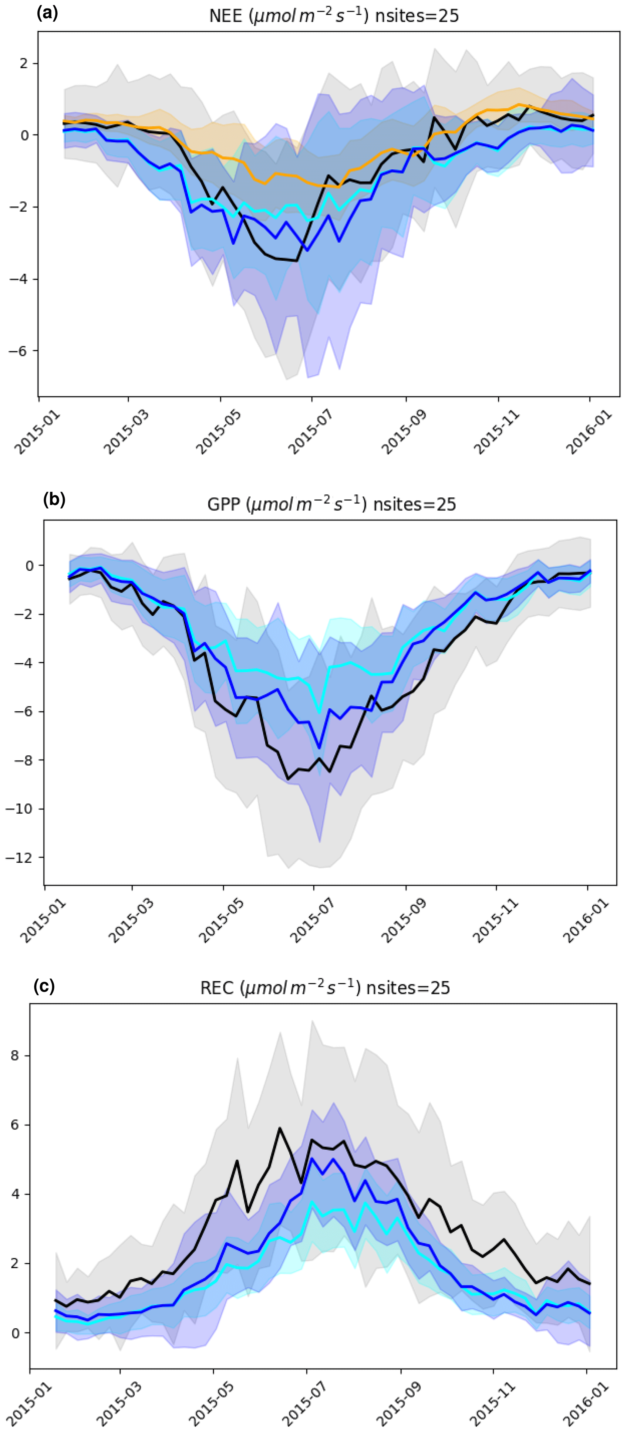
Figure 21Mean seasonal cycle of weekly CO2 biogenic fluxes µmol [m−2 s−1] from ERA5-Land (in cyan), bias-corrected ERA5-Land (in blue), and the CAMS atmospheric in situ inversion product (v18r3, https://atmosphere.copernicus.eu/data, last access: 27 August 2021, Chevallier et al., 2010) minus fossil fuel emissions (in orange) for 2015 at 25 ICOS-ETC sites over Europe (in black) (ICOS-ETC Drought 2018 Team, 2019). The shading shows the standard deviation of each dataset across the 25 sites. (a) NEE; (b) GPP; (c) ecosystem respiration (Reco).
Another important research path with large potential is the revision and use of dynamic auxiliary data. Currently, ERA5-Land assumes a fixed land cover, whereas leaf area index (LAI) and albedo are based on a static monthly climatology. The former assumes that land cover remains unaltered for the complete reanalysis period and that cities are non existent, whereas the latter will not be able to accurately represent more frequent LAI anomalies. Based on the research conducted in the ESA-CCI programme, C3S provides (through the CDS) climate data records of land cover at yearly frequency, as well as a close-to-real-time global map of LAI with 10 to 20 d latency. Moreover, recent studies have identified errors in the diurnal cycle of land surface temperature over the Iberian Peninsula associated with the current land cover used in CHTESSEL and 1 h model time steps (Johannsen et al., 2019; Nogueira et al., 2020). Therefore, the revision of the land cover and LAI to a new database as well as the introduction of their interannual variability is expected to provide more realistic land conditions as input to the surface scheme. There are also ongoing efforts to revise the vertical discretization of the vegetation roots and soil layers distribution (e.g. Mueller-Quintino et al., 2016; Stevens et al., 2020), which could complement the land cover and vegetation updates.
Finally, the coupling of the offline simulations to an offline data assimilation system is a promising approach. The advantages are multiple, in particular the assimilation of local datasets (precipitation radar observations, local soil moisture networks, etc.), permitting small adjustments of land state estimates. Undoubtedly, this will go accompanied by an increase in computational cost. Ongoing efforts to improve the parallelization of the land model will allow global high-resolution simulations for several decades to be performed at affordable computational costs.
All the components discussed above are currently under research, but they are not the only ones. ECMWF is currently working with a flexible, modular system called ECLand (Boussetta et al., 2021) which allows us to separately develop several modelling aspects of the land surface, such as the increase in the number of soil layers or the introduction of a multi-layer snow scheme, as well as make progress on other longer-term perspectives such as the introduction of a groundwater storage or the reduction of the model time step. All the above ongoing developments will provide the basis for a future new version with improved accuracy for the land states at multi-decadal timescales.
Table A1List of climatological (invariant) fields used as input in the production of ERA5-Land.
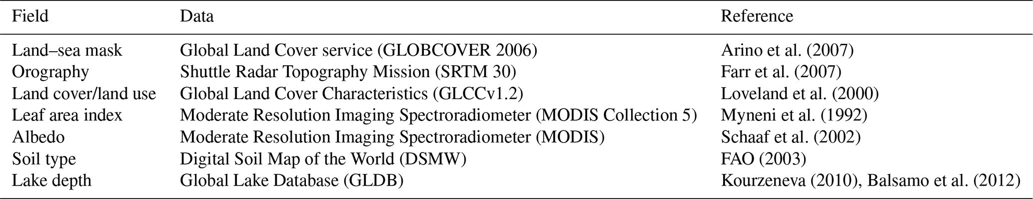
Table A2Portfolio of ERA5-Land data fields available through the Copernicus CDS. The left column shows the atmospheric forcing fields from ERA5 that have been interpolated to the ERA5-Land spatial resolution. The right column shows all fields generated by ERA5-Land. A short description of each field is available in the CDS (Muñoz-Sabater, 2019a, b).
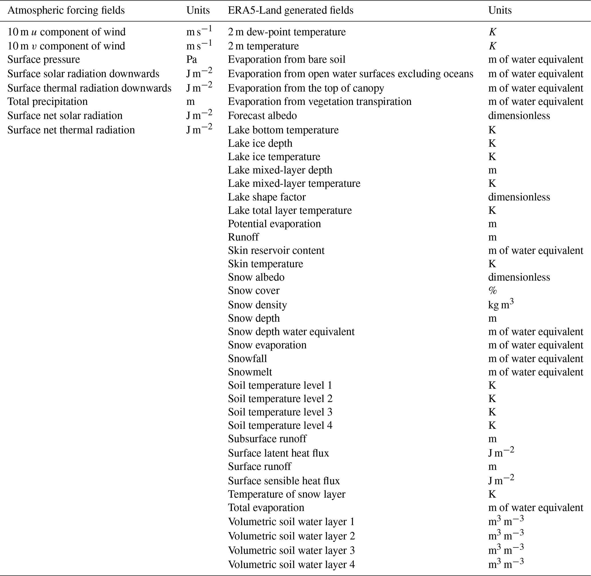
The supplement related to this article is available online at: https://doi.org/10.5194/essd-13-4349-2021-supplement.
JMS produced the ERA5-Land dataset, designed the study, and wrote the paper. ED, GB, SB, HH, DGM, CB, and JNT revised the paper and the figures, wrote some text, and provided a critical review of the paper; CA pre-processed soil moisture data; NJRF conducted the corresponding analysis; GA processed and analysed the snow data; MC collected, processed, and analysed all the lake data of this study; SH and EZ provided the evaluation of the river discharge data; BM processed and evaluated all the surface energy fluxes and ran the GLEAM model; MP collected and evaluated the skin temperature data; AAP processed and produced the bias-corrected carbon flux example. SH also proofread most of the paper.
The authors declare that they have no conflict of interest.
Publisher's note: Copernicus Publications remains neutral with regard to jurisdictional claims in published maps and institutional affiliations.
GloFAS partners and the Global Runoff Data Centre (GRDC), 56068 Koblenz, Germany, are thanked for providing river discharge observations. Laura Rontu and Matti Horttanainen are thanked for providing in situ data for the Finnish lakes. Miguel Potes, Rui Salgado, and Maksim Iakunin are thanked for providing in situ data for the Alqueva reservoir. The authors thank Alex Vermeulen (ICOS Carbon Portal) for his advice on the use of the Drought-2018 ecosystem eddy-covariance flux product in FLUXNET-Archive format – release 2019-1. The contribution of Gabriele Arduini was funded through the APPLICATE project. The APPLICATE has received funding from the European Union's Horizon 2020 research and innovation programme under grant agreement no. 727862.
ERA5-Land was produced with funding from the European Union's Copernicus Climate Change Service.
This paper was edited by Alexander Gruber and reviewed by Wouter Dorigo and one anonymous referee.
Agustí-Panareda, A., Massart, S., Chevallier, F., Balsamo, G., Boussetta, S., Dutra, E., and Beljaars, A.: A biogenic CO2 flux adjustment scheme for the mitigation of large-scale biases in global atmospheric CO2 analyses and forecasts, Atmos. Chem. Phys., 16, 10399–10418, https://doi.org/10.5194/acp-16-10399-2016, 2016. a
Albergel, C., Balsamo, G., de Rosnay, P., Muñoz-Sabater, J., and Boussetta, S.: A bare ground evaporation revision in the ECMWF land-surface scheme: evaluation of its impact using ground soil moisture and satellite microwave data, Hydrol. Earth Syst. Sci., 16, 3607–3620, https://doi.org/10.5194/hess-16-3607-2012, 2012. a
Albergel, C., Munier, S., Leroux, D. J., Dewaele, H., Fairbairn, D., Barbu, A. L., Gelati, E., Dorigo, W., Faroux, S., Meurey, C., Le Moigne, P., Decharme, B., Mahfouf, J.-F., and Calvet, J.-C.: Sequential assimilation of satellite-derived vegetation and soil moisture products using SURFEX_v8.0: LDAS-Monde assessment over the Euro-Mediterranean area, Geosci. Model Dev., 10, 3889–3912, https://doi.org/10.5194/gmd-10-3889-2017, 2017. a
Arino, O., Gross, D., Ranera, F., Leroy, M., Bicheron, P., Brockman, C., Defourny, P., Vancutsem, C., Achard, F., Durieux, L., Bourg, L., Latham, J., Di Gregorio, A., Witt, R., Herold, M., Sambale, J., Plummer, S., and Weber, J.: GlobCover: ESA service for global land cover from MERIS, IEEE Int. Geosci. Remote Se., 2007, 2412–2415, https://doi.org/10.1109/IGARSS.2007.4423328, 2007. a
Balsamo, G., Dutra, E., Stepanenko, V., Viterbo, P., Miranda, P., and Mironov, D.: Deriving an Effective Lake Depth from Satellite Lake Surface Temperature: A Feasibility Study with MODIS Data, Boreal Environ. Res., 15, 178–190, 2010. a
Balsamo, G., Salgado, R., Dutra, E., Boussetta, S., Stockdale, T., and Potes, M.: On the contribution of lakes in predicting near-surface temperature in a global weather forecasting model, Tellus A, 64, 15829, https://doi.org/10.3402/tellusa.v64i0.15829, 2012. a, b
Balsamo, G., Albergel, C., Beljaars, A., Boussetta, S., Brun, E., Cloke, H., Dee, D., Dutra, E., Muñoz-Sabater, J., Pappenberger, F., de Rosnay, P., Stockdale, T., and Vitart, F.: ERA-Interim/Land: a global land surface reanalysis data set, Hydrol. Earth Syst. Sci., 19, 389–407, https://doi.org/10.5194/hess-19-389-2015, 2015. a, b
Beck, H. E., Pan, M., Roy, T., Weedon, G. P., Pappenberger, F., van Dijk, A. I. J. M., Huffman, G. J., Adler, R. F., and Wood, E. F.: Daily evaluation of 26 precipitation datasets using Stage-IV gauge-radar data for the CONUS, Hydrol. Earth Syst. Sci., 23, 207–224, https://doi.org/10.5194/hess-23-207-2019, 2019. a
Beck, H. E., Pan, M., Miralles, D. G., Reichle, R. H., Dorigo, W. A., Hahn, S., Sheffield, J., Karthikeyan, L., Balsamo, G., Parinussa, R. M., van Dijk, A. I. J. M., Du, J., Kimball, J. S., Vergopolan, N., and Wood, E. F.: Evaluation of 18 satellite- and model-based soil moisture products using in situ measurements from 826 sensors, Hydrol. Earth Syst. Sci., 25, 17–40, https://doi.org/10.5194/hess-25-17-2021, 2021. a
Bell, B., Hersbach, H., Simmons, A., Berrisford, P., Dahlgren, P., Horanyi, A., Muñoz Sabater, J., Nicolas, J., Radu, R., Schepers, D., Soci, C., Bidlot, J., Haimberger, L., and Woollen, J.: The ERA5 Global Reanalysis: Extension to 1950, Q. J. Roy. Meteor. Soc., accepted, 2021. a
Bell, J., Palecki, M., Baker, C., Collins, W., Lawrimore, J., Leeper, R., Hall, M., Kochendorfer, J., Meyers, T., Wilson, T., and Diamond, H.: U.S. Climate Reference Network soil moisture and temperature observations, J. Hydrometeorol., 14, 977–988, 2013. a
Bircher, S., Skou, N., Jensen, K. H., Walker, J. P., and Rasmussen, L.: A soil moisture and temperature network for SMOS validation in Western Denmark, Hydrol. Earth Syst. Sci., 16, 1445–1463, https://doi.org/10.5194/hess-16-1445-2012, 2012. a
Boussetta, S., Balsamo, G., Beljaars, A., Agusti-Panareda, A., Calvet, J., Jacobs, C., van den Hurk, B., Viterbo, P., Lafont, S., Dutra, E., Jarlan, L., Balzarolo, M., Papale, D., and van der Werf, G.: Natural land carbon dioxide exchanges in the ECMWF Integrated Forecasting System: Implementation and offline validation, J. Geophys. Res., 118, 5923–5946, https://doi.org/10.1002/jgrd.50488, 2013a. a, b, c
Boussetta, S., Balsamo, G., Beljaars, A., Kral, T., and Jarlan, L.: Impact of a satellite-derived leaf area index monthly climatology in a global numerical weather prediction model, Int. J. Remote Sens., 34, 3520–3542, https://doi.org/10.1080/01431161.2012.716543, 2013b. a
Boussetta, S., Balsamo, G., Arduini, G., Dutra, E., McNorton, J., Choulga, M., Agustí-Panareda, A., Beljaars, A., Wedi, N., Muñoz Sabater, J., de Rosnay, P., Sandu, I., Hadade, I., Carver, G., Mazzetti, C., Prudhomme, C., Yamazaki, D., and Zsoter, E.: ECLand: The ECMWF Land Surface Modelling System, Atmosphere, 12, 723, https://doi.org/10.3390/atmos12060723, 2021. a, b
Calvet, J., Noilhan, J., Roujean, J.-L., Bessemoulin, P., Cabelguenne, M., Olioso, A., and Wigneron, J.-P.: An interactive vegetation SVAT model tested against data from six contrasting sites, Agr. Forest Meteorol., 92, 73–95, 1998. a
Calvet, J.-C., Fritz, N., Froissard, F., Suquia, D., Petitpa, A., and Piguet, B.: In situ soil moisture observations for the CAL/VAL of SMOS: The SMOSMANIA network, IEEE Int. Geosci. Remote Se., 2007, 1196–1199, 2007. a
Cao, B., Gruber, S., Zheng, D., and Li, X.: The ERA5-Land soil temperature bias in permafrost regions, The Cryosphere, 14, 2581–2595, https://doi.org/10.5194/tc-14-2581-2020, 2020. a
Chen, X., Su, Z., Ma, Y., Cleverly, J., and Liddell, M.: An Accurate Estimate of Monthly Mean Land Surface Temperatures from MODIS Clear-Sky Retrievals, J. Hydrometeorol., 18, 2827–2847, https://doi.org/10.1175/JHM-D-17-0009.1, 2017. a, b
Chevallier, F., Ciais, P., Conway, T. J., Aalto, T., Anderson, B. E., Bousquet, P., Brunke, E. G., Ciattaglia, L., Esaki, Y., Fröhlich, M., Gomez, A., Gomez-Pelaez, A. J., Haszpra, L., Krummel, P. B., Langenfelds, R. L., Leuenberger, M., Machida, T., Maignan, F., Matsueda, H., Morguí, J. A., Mukai, H., Nakazawa, T., Peylin, P., Ramonet, M., Rivier, L., Sawa, Y., Schmidt, M., Steele, L. P., Vay, S. A., Vermeulen, A. T., Wofsy, S., and Worthy, D.: CO2 surface fluxes at grid point scale estimated from a global 21 year reanalysis of atmospheric measurements, J. Geophys. Res.-Atmos., 115, D21307, https://doi.org/10.1029/2010JD013887, 2010. a, b
Copernicus Climate Change Service: UERRA Regional Reanalysis for Europe on Single Levels from 1961 to 2019 [data set], available at: https://cds.climate.copernicus.eu/cdsapp#!/dataset/reanalysis-uerra-europe-single-levels?tab=form (last access: 12 February 2021), 2020. a
Courtier, P., Thépaut, J.-N., and Hollingsworth, A.: A strategy for operational implementation of 4D-Var, using an incremental approach, Q. J. Roy. Meteor. Soc., 120, 1367–1387, 1994. a
Cucchi, M., Weedon, G. P., Amici, A., Bellouin, N., Lange, S., Müller Schmied, H., Hersbach, H., and Buontempo, C.: WFDE5: bias-adjusted ERA5 reanalysis data for impact studies, Earth Syst. Sci. Data, 12, 2097–2120, https://doi.org/10.5194/essd-12-2097-2020, 2020. a
de Rosnay, P., Drusch, M., Vasiljevic, D., Balsamo, G., Albergel, C., and Isaksen, L.: A simplified Extended Kalman Filter for the global operational soil moisture analysis at ECMWF, Q. J. Roy. Meteor. Soc., 139, 1199–1213, 2013. a
de Rosnay, P., Isaksen, L., and Dahoui, M.: Snow data assimilation at ECMWF, ECMWF Newsletter, 143, 26–31, https://doi.org/10.21957/lkpxq6x5, 2015. a
Dee, D. P., Uppala, S. M., Simmons, A. J., Berrisford, P., Poli, P., Kobayashi, S., Andrae, U., Balmaseda, M. A., Balsamo, G., Bauer, P., Bechtold, P., Beljaars, A. C. M., van de Berg, L., Bidlot, J., Bormann, N., Delsol, C., Dragani, R., Fuentes, M., Geer, A. J., Haimberger, L., Healy, S. B., Hersbach, H., Hólm, E. V., Isaksen, L., Kållberg, P., Köhler, M., Matricardi, M., McNally, A. P., Monge-Sanz, B. M., Morcrette, J.-J., Park, B.-K., Peubey, C., de Rosnay, P., Tavolato, C., Thépaut, J.-N., and Vitart, F.: The ERA-Interim reanalysis: configuration and performance of the data assimilation system, Q. J. Roy. Meteor. Soc., 137, 553–597, https://doi.org/10.1002/qj.828, 2011. a, b
Dirmeyer, P. and Tan, L.: A multi-decadal global land-surface data set of state variables and fluxes, Tech. rep., COLA 102, 43 pp., Center for Ocean–Land–Atmosphere Studies, 4041 Powder Mill Road, Suite 302, Calverton, MD 20705, 2001. a
Dirmeyer, P. A., Dolman, A. J., and Sato, N.: The Pilot Phase of the Global Soil Wetness Project, B. Am. Meteorol. Soc., 80, 851–878, https://doi.org/10.1175/1520-0477(1999)080<0851:TPPOTG>2.0.CO;2, 1999. a
Dorigo, W. A., Wagner, W., Hohensinn, R., Hahn, S., Paulik, C., Xaver, A., Gruber, A., Drusch, M., Mecklenburg, S., van Oevelen, P., Robock, A., and Jackson, T.: The International Soil Moisture Network: a data hosting facility for global in situ soil moisture measurements, Hydrol. Earth Syst. Sci., 15, 1675–1698, https://doi.org/10.5194/hess-15-1675-2011, 2011. a, b
Dorigo, W., Himmelbauer, I., Aberer, D., Schremmer, L., Petrakovic, I., Zappa, L., Preimesberger, W., Xaver, A., Annor, F., Ardö, J., Baldocchi, D., Blöschl, G., Bogena, H., Brocca, L., Calvet, J.-C., Camarero, J. J., Capello, G., Choi, M., Cosh, M. C., Demarty, J., van de Giesen, N., Hajdu, I., Jensen, K. H., Kanniah, K. D., de Kat, I., Kirchengast, G., Rai, P. K., Kyrouac, J., Larson, K., Liu, S., Loew, A., Moghaddam, M., Martínez Fernández, J., Mattar Bader, C., Morbidelli, R., Musial, J. P., Osenga, E., Palecki, M. A., Pfeil, I., Powers, J., Ikonen, J., Robock, A., Rüdiger, C., Rummel, U., Strobel, M., Su, Z., Sullivan, R., Tagesson, T., Vreugdenhil, M., Walker, J., Wigneron, J. P., Woods, M., Yang, K., Zhang, X., Zreda, M., Dietrich, S., Gruber, A., van Oevelen, P., Wagner, W., Scipal, K., Drusch, M., and Sabia, R.: The International Soil Moisture Network: serving Earth system science for over a decade, Hydrol. Earth Syst. Sci. Discuss. [preprint], https://doi.org/10.5194/hess-2021-2, in review, 2021. a, b
Douville, H., Viterbo, P., Mahfouf, J.-F., and Beljaars, A. C. M.: Evaluation of the Optimum Interpolation and Nudging Techniques for Soil Moisture Analysis Using FIFE Data, Mon. Weather Rev., 128, 1733–1756, https://doi.org/10.1175/1520-0493(2000)128<1733:EOTOIA>2.0.CO;2, 2000. a
Drusch, M., Vasiljevic, D., and Viterbo, P.: ECMWF's Global Snow Analysis: Assessment and Revision Based on Satellite Observations, J. Appl. Meteorol., 43, 1282–1294, https://doi.org/10.1175/1520-0450(2004)043<1282:EGSAAA>2.0.CO;2, 2004. a
Dutra, E., Stepanenko, V., Balsamo, G., Viterbo, P., Miranda, P., Mironov, D., and Schaer, C.: An offline study of the impact of lakes on the performance of the ECMWF surface scheme, Boreal Environ. Res., 15, 100–112, 2010. a, b
Dutra, E., Muñoz-Sabater, J., Boussetta, S., Komori, T., Hirahara, S., and Balsamo, G.: Environmental Lapse Rate for High-Resolution Land Surface Downscaling: An Application to ERA5, Earth Space Sci., 7, e2019EA000984, https://doi.org/10.1029/2019EA000984, 2020. a, b
Ershadi, A., McCabe, M., Evans, J., Chaney, N., and Wood, E.: Multi-site evaluation of terrestrial evaporation models using FLUXNET data, Agr. Forest Meteorol., 187, 46–61, https://doi.org/10.1016/j.agrformet.2013.11.008, 2014. a
Etchevers, P., Martin, E., Brown, R., Fierz, C., Lejeune, Y., Bazile, E., Boone, A., Dai, Y. J., Essery, R., Fernandez, A., Gusev, Y., Jordan, R., Koren, V., Kowalczyk, E., Nasonova, N. O., Pyles, R. D., Schlosser, A., Shmakin, A. B., Smirnova, T. G., Strasser, U., Verseghy, D., Yamazaki, T., and Yang, Z. L.: Validation of the energy budget of an alpine snowpack simulated by several snow models (SnowMIP project), Ann. Glaciol., 38, 150–158, https://doi.org/10.3189/172756404781814825, 2004. a
FAO: Digital Soil Map of the World (DSMW), Tech. rep., Food and Agriculture Organization of the United Nations, re-issued version, available at: http://www.fao.org/soils-portal/data-hub/soil-maps-and-databases/faounesco-soil-map-of-the-world/en/ (last access: 30 August 2021), 2003. a
Farr, T. G., Rosen, P. A., Caro, E., Crippen, R., Duren, R., Hensley, S., Kobrick, M., Paller, M., Rodriguez, E., Roth, L., Seal, D., Shaffer, S., Shimada, J., Umland, J., Werner, M., Oskin, M., Burbank, D., and Alsdorf, D.: The Shuttle Radar Topography Mission, Rev. Geophys., 45, RG2004, https://doi.org/10.1029/2005RG000183, 2007. a
Gomis-Cebolla, J., Jimenez, J. C., and Sobrino, J. A.: LST retrieval algorithm adapted to the Amazon evergreen forests using MODIS data, Remote Sens. Environ., 204, 401–411, https://doi.org/10.1016/j.rse.2017.10.015, 2018. a
Gruber, A., De Lannoy, G., Albergel, C., Al-Yaari, A., Brocca, L., Calvet, J.-C., Colliander, A., Cosh, M., Crow, W., Dorigo, W., Draper, C., Hirschi, M., Kerr, Y., Konings, A., Lahoz, W., McColl, K., Montzka, C., Muñoz-Sabater, J., Peng, J., Reichle, R., Richaume, P., Rüdiger, C., Scanlon, T., van der Schalie, R., Wigneron, J.-P., and Wagner, W.: Validation practices for satellite soil moisture retrievals: What are (the) errors?, Remote Sens. Environ., 244, 111806, https://doi.org/10.1016/j.rse.2020.111806, 2020. a
Gupta, H. V., Kling, H., Yilmaz, K. K., and Martinez, G. F.: Decomposition of the mean squared error and NSE performance criteria: Implications for improving hydrological modelling, J. Hydrol., 377, 80–91, https://doi.org/10.1016/j.jhydrol.2009.08.003, 2009. a
Harding, R., Best, M., Blyth, E., Hagemann, S., Kabat, P., Tallaksen, L. M., Warnaars, T., Wiberg, D., Weedon, G. P., Van Lanen, H., Ludwig, F., and Haddeland, I.: WATCH: Current knowledge of the terrestrial global water cycle, J. Hydrometeorol., 12, 1149–1156, https://doi.org/10.1175/JHM-D-11-024.1, 2011. a
Harrigan, S., Zsoter, E., Barnard, C., Wetterhall F., Salamon, P., and Prudhomme, C.: River discharge and related historical data from the Global Flood Awareness System, v2.1, Copernicus Climate Change Service (C3S) Climate Data Store (CDS) [data set], https://doi.org/10.24381/cds.a4fdd6b9, 2019. a
Harrigan, S., Zsoter, E., Alfieri, L., Prudhomme, C., Salamon, P., Wetterhall, F., Barnard, C., Cloke, H., and Pappenberger, F.: GloFAS-ERA5 operational global river discharge reanalysis 1979–present, Earth Syst. Sci. Data, 12, 2043–2060, https://doi.org/10.5194/essd-12-2043-2020, 2020. a, b, c
Henderson-Sellers, A., Pitman, A. J., Love, P. K., Irannejad, P., and Chen, T. H.: The Project for Intercomparison of Land Surface Parameterization Schemes (PILPS): Phases 2 and 3*, B. Am. Meteorol. Soc., 76, 489–504, https://doi.org/10.1175/1520-0477(1995)076<0489:TPFIOL>2.0.CO;2, 1995. a
Hersbach, H., Bell, B., Berrisford, P., Biavati, G., Horányi, A., Muñoz Sabater, J., Nicolas, J., Peubey, C., Radu, R., Rozum, I., Schepers, D., Simmons, A., Soci, C., Dee, D., and Thépaut, J.-N.: ERA5-Land hourly data from 1981 to present, Copernicus Climate Change Service (C3S) Climate Data Store (CDS) [data set], https://doi.org/10.24381/cds.adbb2d47, 2018. a
Hersbach, H., Bell, B., Berrisford, P., Hirahara, S., Horányi, A., Muñoz-Sabater, J., Nicolas, J., Peubey, C., Radu, R., Schepers, D., Simmons, A., Soci, C., Abdalla, S., Abellan, X., Balsamo, G., Bechtold, P., Biavati, G., Bidlot, J., Bonavita, M., De Chiara, G., Dahlgren, P., Dee, D., Diamantakis, M., Dragani, R., Flemming, J., Forbes, R., Fuentes, M., Geer, A., Haimberger, L., Healy, S., Hogan, R. J., Hólm, E., Janisková, M., Keeley, S., Laloyaux, P., Lopez, P., Lupu, C., Radnoti, G., de Rosnay, P., Rozum, I., Vamborg, F., Villaume, S., and Thépaut, J.-N.: The ERA5 global reanalysis, Q. J. Roy. Meteor. Soc., 146, 1999–2049, https://doi.org/10.1002/qj.3803, 2020. a, b, c, d
ICOS-ETC Drought 2018 Team: Drought-2018 ecosystem eddy covariance flux product in FLUXNET-Archive format – release 2019-1 (Version 1.0), ICOS Carbon Portal, https://doi.org/10.18160/PZDK-EF78, 2019. a, b, c
Ikonen, J., Vehviläinen, J., Rautiainen, K., Smolander, T., Lemmetyinen, J., Bircher, S., and Pulliainen, J.: The Sodankylä in situ soil moisture observation network: an example application of ESA CCI soil moisture product evaluation, Geosci. Instrum. Method. Data Syst., 5, 95–108, https://doi.org/10.5194/gi-5-95-2016, 2016. a
Jacobs, C., van den Hurk, B., and de Bruin, H.: Stomatal behaviour and photosynthetic rate of unstressed grapevines in semi-arid conditions, Agr. Forest Meteorol., 80, 111–134, https://doi.org/10.1016/0168-1923(95)02295-3, 1996. a
Jarvis, P. G., Monteith, J. L., and Weatherley, P. E.: The interpretation of the variations in leaf water potential and stomatal conductance found in canopies in the field, Philos. T. R. Soc. Lon. B, 273, 593–610, https://doi.org/10.1098/rstb.1976.0035, 1976. a
Jensen, N. and Barrett, C.: Agricultural Index Insurance for Development, Appl. Econ. Perspect. P., 39, 199–219, https://doi.org/10.1093/aepp/ppw022, 2016. a
Jiménez, C., Martens, B., Miralles, D. M., Fisher, J. B., Beck, H. E., and Fernández-Prieto, D.: Exploring the merging of the global land evaporation WACMOS-ET products based on local tower measurements, Hydrol. Earth Syst. Sci., 22, 4513–4533, https://doi.org/10.5194/hess-22-4513-2018, 2018. a
Jiménez-Muñoz, J. C., Mattar, C., Sobrino, J. A., and Malhi, Y.: Digital thermal monitoring of the Amazon forest: an intercomparison of satellite and reanalysis products, Int. J. Digit. Earth, 9, 477–498, https://doi.org/10.1080/17538947.2015.1056559, 2016. a
Johannsen, F., Ermida, S., Martins, J. P. A., Trigo, I. F., Nogueira, M., and Dutra, E.: Cold Bias of ERA5 Summertime Daily Maximum Land Surface Temperature over Iberian Peninsula, Remote Sensing, 11, 2570, https://doi.org/10.3390/rs11212570, 2019. a
Jung, M., Schwalm, C., Migliavacca, M., Walther, S., Camps-Valls, G., Koirala, S., Anthoni, P., Besnard, S., Bodesheim, P., Carvalhais, N., Chevallier, F., Gans, F., Goll, D. S., Haverd, V., Köhler, P., Ichii, K., Jain, A. K., Liu, J., Lombardozzi, D., Nabel, J. E. M. S., Nelson, J. A., O'Sullivan, M., Pallandt, M., Papale, D., Peters, W., Pongratz, J., Rödenbeck, C., Sitch, S., Tramontana, G., Walker, A., Weber, U., and Reichstein, M.: Scaling carbon fluxes from eddy covariance sites to globe: synthesis and evaluation of the FLUXCOM approach, Biogeosciences, 17, 1343–1365, https://doi.org/10.5194/bg-17-1343-2020, 2020. a
Karger, D. N., Conrad, O., Böhner, J., Kawohl, T., Kreft, H., Soria-Auza, R. W., Zimmermann, N. E., Linder, H. P., and Kessler, M.: Climatologies at high resolution for the earth's land surface areas, Sci. Data, 5, 170122, https://doi.org/10.1038/sdata.2017.122, 2017. a
Kling, H., Fuchs, M., and Paulin, M.: Runoff conditions in the upper Danube basin under an ensemble of climate change scenarios, J. Hydrol., 424–425, 264–277, https://doi.org/10.1016/j.jhydrol.2012.01.011, 2012. a
Koster, R. D., Dirmeyer, P. A., Guo, Z., Bonan, G., Chan, E., Cox, P., Gordon, C. T., Kanae, S., Kowalczyk, E., Lawrence, D., Liu, P., Lu, C.-H., Malyshev, S., McAvaney, B., Mitchell, K., Mocko, D., Oki, T., Oleson, K., Pitman, A., Sud, Y. C., Taylor, C. M., Verseghy, D., Vasic, R., Xue, Y., and Yamada, T.: Regions of Strong Coupling Between Soil Moisture and Precipitation, Science, 305, 1138–1140, https://doi.org/10.1126/science.1100217, 2004. a
Kourzeneva, E.: External data for lake parameterization in Numerical Weather Prediction and climate modeling, Boreal Environ. Res, 15, 165–177, 2010. a
Krinner, G., Derksen, C., Essery, R., Flanner, M., Hagemann, S., Clark, M., Hall, A., Rott, H., Brutel-Vuilmet, C., Kim, H., Ménard, C. B., Mudryk, L., Thackeray, C., Wang, L., Arduini, G., Balsamo, G., Bartlett, P., Boike, J., Boone, A., Chéruy, F., Colin, J., Cuntz, M., Dai, Y., Decharme, B., Derry, J., Ducharne, A., Dutra, E., Fang, X., Fierz, C., Ghattas, J., Gusev, Y., Haverd, V., Kontu, A., Lafaysse, M., Law, R., Lawrence, D., Li, W., Marke, T., Marks, D., Ménégoz, M., Nasonova, O., Nitta, T., Niwano, M., Pomeroy, J., Raleigh, M. S., Schaedler, G., Semenov, V., Smirnova, T. G., Stacke, T., Strasser, U., Svenson, S., Turkov, D., Wang, T., Wever, N., Yuan, H., Zhou, W., and Zhu, D.: ESM-SnowMIP: assessing snow models and quantifying snow-related climate feedbacks, Geosci. Model Dev., 11, 5027–5049, https://doi.org/10.5194/gmd-11-5027-2018, 2018. a, b, c
Lafore, J.-P., Flamant, C., Giraud, V., Guichard, F., Knippertz, P., Mahfouf, J.-F., Mascart, P., and Williams, E.: Introduction to the AMMA Special Issue on “Advances in understanding atmospheric processes over West Africa through the AMMA field campaign', Q. J. Roy. Meteor. Soc., 136, 2–7, https://doi.org/10.1002/qj.583, 2010. a
Leavesley, G., David, O., Garen, D., Lea, J., Marron, J., Pagano, T., Perkins, T., and Strobel, M.: A modeling framework for improved agricultural water supply forecasting, in: AGU Fall Meeting Abstracts, Washington, D.C., American Geophysical Union, vol. 1, p. 0497, 2008. a
Lobell, D. B., Schlenker, W., and Costa-Roberts, J.: Climate Trends and Global Crop Production Since 1980, Science, 333, 616–620, https://doi.org/10.1126/science.1204531, 2011. a
Lopez-Baeza, E., Antolin, M., Balling, J. E., Belda, F., Bouzinac, C., Camacho, F., Cano, A., Carbo, E., Delwart, S., Domenech, C., Ferreira, A. G., Fidalgo, A., Juglea, S., Kerr, Y., Marco, J., Millan-Scheiding, C., Narbon, C., Rodriguez, D., Saleh, K., Sanchis, J., Skou, Sten, N., Søbjærg, S., Soriano, P., Tamayo, J., Tauriainen, S., Torre, E., Velazquez-Blazquez, A., Wigneron, J.-P., and Wursteisen, P.: Soil moisture characterization of the Valencia anchor station. Ground, aircraft measurements and simulations, in: Proceedings of the Second EPS/MetOp RAO Workshop, European Space Agency, 2009. a
Loveland, T. R., Reed, B. C., Brown, J. F., Ohlen, D. O., Zhu, Z., Youing, L., and Merchant, J. W.: Development of a global land cover characteristics database and IGB6 DISCover from the 1 km AVHRR data, Int. J. Remote Sens., 21, 1303–1330, 2000. a
MacLeod, D. A., Cloke, H. L., Pappenberger, F., and Weisheimer, A.: Improved seasonal prediction of the hot summer of 2003 over Europe through better representation of uncertainty in the land surface, Q. J. Roy. Meteor. Soc., 142, 79–90, https://doi.org/10.1002/qj.2631, 2016. a
Mahfouf, J.-F.: Analysis of Soil Moisture from Near-Surface Parameters: A Feasibility Study, J. Appl. Meteorol., 30, 1534–1547, https://doi.org/10.1175/1520-0450(1991)030<1534:AOSMFN>2.0.CO;2, 1991. a
Malardel, S., Wedi, N., Deconinck, W., Diamantakis, M., Kuehnlein, C., Mozdzynski, G., Hamrud, M., and Smolarkiewicz, P.: A new grid for the IFS, ECMWF Newsletter, 146, 23–28, https://doi.org/10.21957/zwdu9u5i, 2016. a
Martens, B., Miralles, D. G., Lievens, H., van der Schalie, R., de Jeu, R. A. M., Fernández-Prieto, D., Beck, H. E., Dorigo, W. A., and Verhoest, N. E. C.: GLEAM v3: satellite-based land evaporation and root-zone soil moisture, Geosci. Model Dev., 10, 1903–1925, https://doi.org/10.5194/gmd-10-1903-2017, 2017. a, b, c, d
Martens, B., Schumacher, D. L., Wouters, H., Muñoz-Sabater, J., Verhoest, N. E. C., and Miralles, D. G.: Evaluating the land-surface energy partitioning in ERA5, Geosci. Model Dev., 13, 4159–4181, https://doi.org/10.5194/gmd-13-4159-2020, 2020. a, b, c, d, e, f
Martínez-Fernández, J. and Ceballos, A.: Mean soil moisture estimation using temporal stability analysis, J. Hydrol., 312, 28–38, 2005. a
Ménard, C. and Essery, R.: ESM-SnowMIP meteorological and evaluation datasets at ten reference sites (in situ and bias corrected reanalysis data), PANGAEA [data set], https://doi.org/10.1594/PANGAEA.897575, 2019. a
Ménard, C. B., Essery, R., Barr, A., Bartlett, P., Derry, J., Dumont, M., Fierz, C., Kim, H., Kontu, A., Lejeune, Y., Marks, D., Niwano, M., Raleigh, M., Wang, L., and Wever, N.: Meteorological and evaluation datasets for snow modelling at 10 reference sites: description of in situ and bias-corrected reanalysis data, Earth Syst. Sci. Data, 11, 865–880, https://doi.org/10.5194/essd-11-865-2019, 2019. a, b
Menne, M., Durre, I., Korzeniewski, B., McNeal, S., Thomas, K., Yin, X., Anthony, S., Ray, R., Vose, R., Gleason, B., and T.G., H.: Global Historical Climatology Network – Daily (GHCN-Daily), Version 3.24, NOAA National Climatic Data Center [data set], https://doi.org/10.7289/V5D21VHZ, 2012a. a
Menne, M. J., Durre, I., Vose, R. S., Gleason, B. E., and Houston, T. G.: An overview of the global historical climatology network-daily database, J. Atmos. Ocean. Tech., 29, 897–910, https://doi.org/10.1175/JTECH-D-11-00103.1, 2012b (data available at: https://www.ncdc.noaa.gov/ghcnd-data-access, last access: 30 August 2021). a, b
Miralles, D. G., Gash, J. H., Holmes, T. R. H., de Jeu, R. A. M., and Dolman, A. J.: Global canopy interception from satellite observations, J. Geophys. Res.-Atmos., 115, D16122, https://doi.org/10.1029/2009JD013530, 2010. a
Miralles, D. G., Holmes, T. R. H., De Jeu, R. A. M., Gash, J. H., Meesters, A. G. C. A., and Dolman, A. J.: Global land-surface evaporation estimated from satellite-based observations, Hydrol. Earth Syst. Sci., 15, 453–469, https://doi.org/10.5194/hess-15-453-2011, 2011. a, b, c
Mironov, D., Heise, E., Kourzeneva, E., Ritter, B., Schneider, N., and Terzhevik, A.: Implementation of the lake parameterisation scheme FLake into numerical weather prediction model COSMO, Boreal Environ. Res., 15, 218–230, 2010a. a
Moghaddam, M., Entekhabi, D., Goykhman, Y., Li, K., Liu, M., Mahajan, A., Nayyar, A., Shuman, D., and Teneketzis, D.: A wireless soil moisture smart sensor web using physics-based optimal control: Concept and initial demonstrations, IEEE J. Sel. Top. Appl., 3, 522–535, https://doi.org/10.1109/JSTARS.2010.2052918, 2010b. a
Muñoz-Sabater, J.: ERA5-Land hourly data from 1981 to present, Copernicus Climate Change Service (C3S) Climate Data Store (CDS) [data set], https://doi.org/10.24381/cds.e2161bac, 2019a. a, b, c, d
Muñoz-Sabater, J.: ERA5-Land monthly averaged data from 1981 to present, Copernicus Climate Change Service (C3S) Climate Data Store (CDS) [data set], https://doi.org/10.24381/cds.68d2bb30, 2019b. a, b, c
Mueller-Quintino, A., Dutra, E., Cloke, H. L., Verhoef, A., Balsamo, G., and Pappenberger, F.: Water infiltration and redistribution in Land Surface Models, ECMWF Tech. Mem. 791, https://doi.org/10.21957/ppksejqu9, 2016. a
Myneni, R. B., Hoffman, S., Knyazikhin, Y., Privette, J. L., Glassy, J., Tian, Y., Wang, Y., Song, X., Zhang, Y., Smith, G. R., Lotsch, A., Friedl, M., Morisette, J. T., Votava, P., Nemani, R. R., and Running, S. W.: Global products of vegetation leaf area and fraction absorbed PAR from year one of MODIS data, Remote Sens. Environ., 83, 214–231, 1992. a
Nogueira, M.: Inter-comparison of ERA-5, ERA-interim and GPCP rainfall over the last 40 years: Process-based analysis of systematic and random differences, J. Hydrol., 583, 124632, https://doi.org/10.1016/j.jhydrol.2020.124632, 2020. a
Nogueira, M., Albergel, C., Boussetta, S., Johannsen, F., Trigo, I. F., Ermida, S. L., Martins, J. P. A., and Dutra, E.: Role of vegetation in representing land surface temperature in the CHTESSEL (CY45R1) and SURFEX-ISBA (v8.1) land surface models: a case study over Iberia, Geosci. Model Dev., 13, 3975–3993, https://doi.org/10.5194/gmd-13-3975-2020, 2020. a
Orth, R., Dutra, E., and Pappenberger, F.: Improving Weather Predictability by Including Land Surface Model Parameter Uncertainty, Mon. Weather Rev., 144, 1551–1569, https://doi.org/10.1175/MWR-D-15-0283.1, 2016. a
Pastorello, G., Trotta, C., Canfora, E., Chu, H., Christianson, D., Cheah, Y.-W., Poindexter, C., Chen, J., Elbashandy, A., Humphrey, M., Isaac, P., Polidori, D., Ribeca, A., van Ingen, C., Zhang, L., Amiro, B., Ammann, C., Arain, M. A., Ardö, J., Arkebauer, T., Arndt, S. K., Arriga, N., Aubinet, M., Aurela, M., Baldocchi, D., Barr, A., Beamesderfer, E., Marchesini, L. B., Bergeron, O., Beringer, J., Bernhofer, C., Berveiller, D., Billesbach, D., Black, T. A., Blanken, P. D., Bohrer, G., Boike, J., Bolstad, P. V., Bonal, D., Bonnefond, J.-M., Bowling, D. R., Bracho, R., Brodeur, J., Brümmer, C., Buchmann, N., Burban, B., Burns, S. P., Buysse, P., Cale, P., Cavagna, M., Cellier, P., Chen, S., Chini, I., Christensen, T. R., Cleverly, J., Collalti, A., Consalvo, C., Cook, B. D., Cook, D., Coursolle, C., Cremonese, E., Curtis, P. S., D'Andrea, E., da Rocha, H., Dai, X., Davis, K. J., De Cinti, B., de Grandcourt, A., De Ligne, A., De Oliveira, R. C., Delpierre, N., Desai, A. R., Di Bella, C. M., di Tommasi, P., Dolman, H., Domingo, F., Dong, G., Dore, S., Duce, P., Dufrêne, E., Dunn, A., Dušek, J., Eamus, D., Eichelmann, U., ElKhidir, H. A. M., Eugster, W., Ewenz, C. M., Ewers, B., Famulari, D., Fares, S., Feigenwinter, I., Feitz, A., Fensholt, R., Filippa, G., Fischer, M., Frank, J., Galvagno, M., Gharun, M., Gianelle, D., Gielen, B., Gioli, B., Gitelson, A., Goded, I., Goeckede, M., Goldstein, A. H., Gough, C. M., Goulden, M. L., Graf, A., Griebel, A., Gruening, C., Grünwald, T., Hammerle, A., Han, S., Han, X., Hansen, B. U., Hanson, C., Hatakka, J., He, Y., Hehn, M., Heinesch, B., Hinko-Najera, N., Hörtnagl, L., Hutley, L., Ibrom, A., Ikawa, H., Jackowicz-Korczynski, M., Janouš, D., Jans, W., Jassal, R., Jiang, S., Kato, T., Khomik, M., Klatt, J., Knohl, A., Knox, S., Kobayashi, H., Koerber, G., Kolle, O., Kosugi, Y., Kotani, A., Kowalski, A., Kruijt, B., Kurbatova, J., Kutsch, W. L., Kwon, H., Launiainen, S., Laurila, T., Law, B., Leuning, R., Li, Y., Liddell, M., Limousin, J.-M., Lion, M., Liska, A. J., Lohila, A., López-Ballesteros, A., López-Blanco, E., Loubet, B., Loustau, D., Lucas-Moffat, A., Lüers, J., Ma, S., Macfarlane, C., Magliulo, V., Maier, R., Mammarella, I., Manca, G., Marcolla, B., Margolis, H. A., Marras, S., Massman, W., Mastepanov, M., Matamala, R., Matthes, J. H., Mazzenga, F., McCaughey, H., McHugh, I., McMillan, A. M. S., Merbold, L., Meyer, W., Meyers, T., Miller, S. D., Minerbi, S., Moderow, U., Monson, R. K., Montagnani, L., Moore, C. E., Moors, E., Moreaux, V., Moureaux, C., Munger, J. W., Nakai, T., Neirynck, J., Nesic, Z., Nicolini, G., Noormets, A., Northwood, M., Nosetto, M., Nouvellon, Y., Novick, K., Oechel, W., Olesen, J. E., Ourcival, J.-M., Papuga, S. A., Parmentier, F.-J., Paul-Limoges, E., Pavelka, M., Peichl, M., Pendall, E., Phillips, R. P., Pilegaard, K., Pirk, N., Posse, G., Powell, T., Prasse, H., Prober, S. M., Rambal, S., Rannik, U., Raz-Yaseef, N., Reed, D., de Dios, V. R., Restrepo-Coupe, N., Reverter, B. R., Roland, M., Sabbatini, S., Sachs, T., Saleska, S. R., Sánchez-Cañete, E. P., Sanchez-Mejia, Z. M., Schmid, H. P., Schmidt, M., Schneider, K., Schrader, F., Schroder, I., Scott, R. L., Sedlák, P., Serrano-Ortíz, P., Shao, C., Shi, P., Shironya, I., Siebicke, L., Šigut, L., Silberstein, R., Sirca, C., Spano, D., Steinbrecher, R., Stevens, R. M., Sturtevant, C., Suyker, A., Tagesson, T., Takanashi, S., Tang, Y., Tapper, N., Thom, J., Tiedemann, F., Tomassucci, M., Tuovinen, J.-P., Urbanski, S., Valentini, R., van der Molen, M., van Gorsel, E., van Huissteden, K., Varlagin, A., Verfaillie, J., Vesala, T., Vincke, C., Vitale, D., Vygodskaya, N., Walker, J. P., Walter-Shea, E., Wang, H., Weber, R., Westermann, S., Wille, C., Wofsy, S., Wohlfahrt, G., Wolf, S., Woodgate, W., Li, Y., Zampedri, R., Zhang, J., Zhou, G., Zona, D., Agarwal, D., Biraud, S., Torn, M., and Papale, D.: The FLUXNET2015 dataset and the ONEFlux processing pipeline for eddy covariance data [data set], Sci. Data, 7, 225, https://doi.org/10.1038/s41597-020-0534-3, 2020. a, b
Pelosi, A., Terribile, F., D'Urso, G., and Chirico, G. B.: Comparison of ERA5-Land and UERRA MESCAN-SURFEX Reanalysis Data with Spatially Interpolated Weather Observations for the Regional Assessment of Reference Evapotranspiration, Water, 12, 1669, https://doi.org/10.3390/w12061669, 2020. a
Peters-Lidard, C. D., Blackburn, E., Liang, X., and Wood, E. F.: The effect of soil conductivity parametrization on surface energy fluxes and temperature, J. Atmos. Sci., 55, 1209–1224, https://doi.org/10.1175/1520-0469(1998)055<1209:TEOSTC>2.0.CO;2, 1998. a
Pitman, A. J.: The evolution of, and revolution in, land surface schemes designed for climate models, Int. J. Climatol., 23, 479–510, https://doi.org/10.1002/joc.893, 2003. a
Rabier, F., Järvinen, H., Klinker, E., Mahfouf, J.-F., and Simmons, A.: The ECMWF operational implementation of four-dimensional variational assimilation. I: Experimental results with simplified physics, Q. J. Roy. Meteor. Soc., 126, 1143–1170, https://doi.org/10.1002/qj.49712656415, 2000. a
Reichle, R. H., Koster, R. D., De Lannoy, G. J. M., Forman, B. A., Liu, Q., Mahanama, S. P. P., and Touré, A.: Assessment and Enhancement of MERRA Land Surface Hydrology Estimates, J. Climate, 24, 6322–6338, https://doi.org/10.1175/JCLI-D-10-05033.1, 2011. a
Reichle, R. H., Liu, Q., Koster, R. D., Draper, C. S., Mahanama, S. P. P., and Partyka, G. S.: Land Surface Precipitation in MERRA-2, J. Climate, 30, 1643–1664, https://doi.org/10.1175/JCLI-D-16-0570.1, 2017. a
Schaaf, C., Gao, F., Strahler, A., Lucht, W., Li, X., Tsang, T., Strugnell, N., Zhang, X., Jin, Y., Muller, J.-P., Lewis, P., Barnsley, M., Hobson, P., Disney, M., Roberts, G., Dunderdale, M., Doll, C., d'Entremont, R., Hu, B., Liang, S., Privette, J., and Roy, D.: First operational BRDF, albedo nadir reflectance products from MODIS, Remote Sens. Environ., 83, 135–148, 2002. a
Schaefer, G., Cosh, M., and Jackson, T.: The USDA natural resources conservation service soil climate analysis network (SCAN), J. Atmos. Ocean. Tech., 24, 2073–2077, https://doi.org/10.1175/2007JTECHA930.1, 2007. a
Schellekens, J., Dutra, E., Martínez-de la Torre, A., Balsamo, G., van Dijk, A., Sperna Weiland, F., Minvielle, M., Calvet, J.-C., Decharme, B., Eisner, S., Fink, G., Flörke, M., Peßenteiner, S., van Beek, R., Polcher, J., Beck, H., Orth, R., Calton, B., Burke, S., Dorigo, W., and Weedon, G. P.: A global water resources ensemble of hydrological models: the eartH2Observe Tier-1 dataset, Earth Syst. Sci. Data, 9, 389–413, https://doi.org/10.5194/essd-9-389-2017, 2017. a
Sharma, S., Gray, D., Read, J., Oreilly, C., Schneider, P., Qudrat, A., Gries, C., Stefanoff, S., Hampton, S., Hook, S., Lenters, J., Livingstone, D., McIntyre, P., Adrian, R., Allan, M., Anneville, O., Arvola, L., Austin, J., Bailey, J., Baron, J., Brookes, J., Chen, Y., Daly, R., Dokulil, M., Dong, B., Ewing, K., de Eyto, E., Hamilton, D., Havens, K., Haydon, S., Hetzenauer, H., Heneberry, J., Hetherington, A., Higgins, S., Hixcon, E., Izmest'eva, L., Jones, B., Kangur, K., Kasprzak, P., Koster, O., Kraemer, B., Kumagai, M., Kuusisto, E., Leshkevich, G., May, L., MacIntyre, S., Mueller-Navarra, D., Naumenko, M., Noges, P., Noges, T., Niederhauser, P., North, R., Paterson, A., Plisnier, P., Rigosi, A., Rimmer, A., Rogora, M., Rudstram, L., Rusak, J., Salmaso, N., Samal, N., Schindler, D., Schladow, G., Schmidt, S., Schultz, T., Silow, E., Straile, D., Teubner, K., Verburg, P., Voutilainen, A., Watkinson, A., Weyhenmeyer, G., Williamson, C., and Woo, K.: Globally distributed lake surface water temperatures collected in situ and by satellites; 1985–2009 ver 3, Environmental Data Initiative [data set], https://doi.org/10.6073/pasta/379a6cebee50119df2575c469aba19c5, 2014. a
Simmons, A., Hersbach, H., Muñoz Sabater, J., Nicolas, J., Vamborg, F., Berrisford, P., de Rosnay, P., Willet, K., and Woollen, J.: Low frequency variability and trends in surface air temperature and humidity from ERA5 and other datasets, EMCWF Tech. Mem. 881, https://doi.org/10.21957/ly5vbtbfd, 2021. a
SYKE: Data and Information Centre [data set], available at: http://www.syke.fi/en-US/SYKE_Info/Organisation/Data_and_Information_Centre(3037), last access: 29 August 2021. a
Smith, A. B., Walker, J. P., Western, A. W., Young, R. I., Ellett, K. M., Pipunic, R. C., Grayson, R. B., Siriwardena, L., Chiew, F. H. S., and H, R.: The Murrumbidgee soil moisture monitoring network data set, Water Resour. Res., 48, W07701, https://doi.org/10.1029/2012WR011976, 2012. a
Stevens, D., Miranda, P. M. A., Orth, R., Boussetta, S., Balsamo, G., and Dutra, E.: Sensitivity of Surface Fluxes in the ECMWF Land Surface Model to the Remotely Sensed Leaf Area Index and Root Distribution: Evaluation with Tower Flux Data, Atmosphere, 11, 1362, https://doi.org/10.3390/atmos11121362, 2020. a
Tadesse, M. A., Shiferaw, B. A., and Erenstein, O.: Weather index insurance for managing drought risk in smallholder agriculture: lessons and policy implications for sub-Saharan Africa, Agricultural and Food Economics, 3, 26, https://doi.org/10.1186/s40100-015-0044-3, 2015. a
Tagesson, T., Fensholt, R., Guiro, I., Rasmussen, M. O., Huber, S., Mbow, C., Garcia, M., Horion, S., Sandholt, I., Holm-Rasmussen, B., Göttsche, F. M., Ridler, M.-E., Olén, N., Lundegard Olsen, J., Ehammer, A., Madsen, M., Olesen, F. S., and Ardö, J.: Ecosystem properties of semiarid savanna grassland in West Africa and its relationship with environmental variability, Glob. Change Biol., 21, 250–264, https://doi.org/10.1111/gcb.12734, 2015. a
Tallec, G., Ansart, P., Guérin, A., Delaigue, O., and Blanchouin, A.: Observatoire Oracle, Irstea. [data set], https://doi.org/10.17180/OBS.ORACLE, 2015. a
Tarek, M., Brissette, F. P., and Arsenault, R.: Evaluation of the ERA5 reanalysis as a potential reference dataset for hydrological modelling over North America, Hydrol. Earth Syst. Sci., 24, 2527–2544, https://doi.org/10.5194/hess-24-2527-2020, 2020. a
van den Hurk, B., Viterbo, P., Beljaars, A., and Betts, A.: Offline validation of the ERA40 surface scheme, ECMWF Tech. Mem. 295, https://doi.org/10.21957/9aoaspz8, 2000. a
van den Hurk, B., Kim, H., Krinner, G., Seneviratne, S. I., Derksen, C., Oki, T., Douville, H., Colin, J., Ducharne, A., Cheruy, F., Viovy, N., Puma, M. J., Wada, Y., Li, W., Jia, B., Alessandri, A., Lawrence, D. M., Weedon, G. P., Ellis, R., Hagemann, S., Mao, J., Flanner, M. G., Zampieri, M., Materia, S., Law, R. M., and Sheffield, J.: LS3MIP (v1.0) contribution to CMIP6: the Land Surface, Snow and Soil moisture Model Intercomparison Project – aims, setup and expected outcome, Geosci. Model Dev., 9, 2809–2832, https://doi.org/10.5194/gmd-9-2809-2016, 2016. a
Van Der Knijff, J., Younis, J., and De Roo, A.: LISFLOOD: a GIS-based distributed model for river basin scale water balance and flood simulation, Int. J. Geogr. Inf. Sci., 24, 189–212, https://doi.org/10.1080/13658810802549154, 2010. a
Vereecken, H., Weihermüller, L., Assouline, S., Šimůnek, J., Verhoef, A., Herbst, M., Archer, N., Mohanty, B., Montzka, C., Vanderborght, J., Balsamo, G., Bechtold, M., Boone, A., Chadburn, S., Cuntz, M., Decharme, B., Ducharne, A., Ek, M., Garrigues, S., Goergen, K., Ingwersen, J., Kollet, S., Lawrence, D. M., Li, Q., Or, D., Swenson, S., de Vrese, P., Walko, R., Wu, Y., and Xue, Y.: Infiltration from the Pedon to Global Grid Scales: An Overview and Outlook for Land Surface Modeling, Vadose Zone J., 18, 180191, https://doi.org/10.2136/vzj2018.10.0191, 2019. a
Wan, Z., Hook, S., and Hulley, G.: MYD11C3 MODIS/Aqua Land Surface Temperature/Emissivity Monthly L3 Global 0.05Deg CMG V006, NASA EOSDIS Land Processes DAAC [data set], https://doi.org/10.5067/MODIS/MYD11C3.006, 2015. a
Weedon, G. P., Gomes, S., Viterbo, P., Shuttleworth, W. J., Blyth, E., ÖSterle, H., Adam, J. C., Bellouin, N., Boucher, O., and Best, M.: Creation of the WATCH forcing data and its use to assess global and regional reference crop evaporation over land during the twentieth century, J. Hydrometeorol., 12, 823–848, https://doi.org/10.1175/2011JHM1369.1, 2011. a
Wheeler, T. and von Braun, J.: Climate Change Impacts on Global Food Security, Science, 341, 508–513, https://doi.org/10.1126/science.1239402, 2013. a
Wilson, K., Goldstein, A., Falge, E., Aubinet, M., Baldocchi, D., Berbigier, P., Bernhofer, C., Ceulemans, R., Dolman, H., Field, C., Grelle, A., Ibrom, A., Law, B., Kowalski, A., Meyers, T., Moncrieff, J., Monson, R., Oechel, W., Tenhunen, J., Valentini, R., and Verma, S.: Energy balance closure at FLUXNET sites, Agr. Forest Meteorol., 113, 223–243, https://doi.org/10.1016/S0168-1923(02)00109-0, 2002. a
Young, R., Walker, J., Yeoh, N., Smith, A., Ellett, K., Merlin, O., and Western, A.: Soil Moisture and Meteorological Observations From the Murrumbidgee Catchment, Tech. rep., Department of Civil and Environmental Engineering, The University of Melbourne, 2008. a
Zacharias, S., Bogena, H., Samaniego, L., Mauder, M., Fuß, R., Pütz, T., Frenzel, M., Schwank, M., Baessler, C., Butterbach-Bahl, K., Bens, O., Borg, E., Brauer, A., Dietrich, P., Hajnsek, I., Helle, G., Kiese, R., Kunstmann, H., Klotz, S., Munch, J.C., Papen, H., Priesack, E., Schmid, H.P., Steinbrecher, R., Rosenbaum, U., Teutsch, G., and Vereecken, H.: A network of terrestrial environmental observatories in Germany, Vadose Zone J., 10, 955–973, https://doi.org/10.2136/VZJ2010.0139, 2011. a
Zhao, C., Liu, B., Piao, S., Wang, X., Lobell, D. B., Huang, Y., Huang, M., Yao, Y., Bassu, S., Ciais, P., Durand, J.-L., Elliott, J., Ewert, F., Janssens, I. A., Li, T., Lin, E., Liu, Q., Martre, P., Müller, C., Peng, S., Peñuelas, J., Ruane, A. C., Wallach, D., Wang, T., Wu, D., Liu, Z., Zhu, Y., Zhu, Z., and Asseng, S.: Temperature increase reduces global yields of major crops in four independent estimates, P. Natl. Acad. Sci. USA, 114, 9326–9331, https://doi.org/10.1073/pnas.1701762114, 2017. a
Zsoter, E., Cloke, H., Stephens, E., de Rosnay, P., Muñoz-Sabater, J., Prudhomme, C., and Pappenberger, F.: How well do operational numerical weather prediction configurations represent hydrology?, J. Hydrometeorol., 20, 1533–1552, https://doi.org/10.1175/JHM-D-18-0086.1, 2019. a, b
- Abstract
- Introduction
- Methodology
- Data and evaluation strategy
- Evaluation results
- Data availability
- Discussion and conclusions
- Perspectives
- Appendix A: List of ERA5-Land input and output fields
- Author contributions
- Competing interests
- Disclaimer
- Acknowledgements
- Financial support
- Review statement
- References
- Supplement