An all-sky 1 km daily land surface air temperature product over mainland China for 2003–2019 from MODIS and ancillary data

Surface air temperature (T_a), as an important climate variable, has been used in a wide range of fields such as ecology, hydrology, climatology, epidemiology, and environmental science. However, ground measurements are limited by poor spatial representation and inconsistency, and reanalysis and meteorological forcing datasets suffer from coarse spatial resolution and inaccuracy. Previous studies using satellite data have mainly estimated T_a under clear-sky conditions or with limited temporal and spatial coverage. In this study, an all-sky daily mean land T_a product at a 1 km spatial resolution over mainland China for 2003–2019 has been generated mainly from the Moderate Resolution Imaging Spectroradiometer (MODIS) products and the Global Land Data Assimilation System (GLDAS) dataset. Three T_a estimation models based on random forest were trained using ground measurements from 2384 stations for three different clear-sky and cloudy-sky conditions. The random sample validation results showed that the R² and root-mean-square error (RMSE) values of the three models ranged from 0.984 to 0.986 and from 1.342 to 1.440 K, respectively. We examined the spatiotemporal patterns and land cover type dependences of model accuracy. Two cross-validation (CV) strategies of leave-time-out (LTO) CV and leave-location-out (LLO) CV were also used to evaluate the models. Finally, we developed the all-sky T_a dataset from 2003 to 2009 and compared it with the China Land Data Assimilation System (CLDAS) dataset at a 0.0625^∘ spatial resolution, the China Meteorological Forcing Data (CMFD) dataset at a 0.1^∘ spatial resolution, and the GLDAS dataset at a 0.25^∘ spatial resolution. Validation accuracy of our product in 2010 was significantly better than other datasets, with R² and RMSE values of 0.992 and 1.010 K, respectively. In summary, the developed all-sky daily mean land T_a dataset has achieved satisfactory accuracy and high spatial resolution simultaneously, which fills the current dataset gap in this field and plays an important role in the studies of climate change and the hydrological cycle. This dataset is currently freely available at https://doi.org/10.5281/zenodo.4399453 (Chen et al., 2021b) and the University of Maryland (http://glass.umd.edu/Ta_China/, last access: 24 August 2021). A sub-dataset that covers Beijing generated from this dataset is also publicly available at https://doi.org/10.5281/zenodo.4405123 (Chen et al., 2021a).

1 Introduction

Surface air temperature (T_a) is one of the most important variables in a wide range of fields including ecology, hydrology, climatology, epidemiology, and environmental science (Goetz et al., 2000; Stisen et al., 2007; Vancutsem et al., 2010; Zhang et al., 2018). T_a refers to the atmospheric temperature 1.5–2 m above the surface, which represents the thermal state information of the surface and the lower atmosphere. It influences the carbon cycle through the biophysical effects of vegetation and regulates many surface processes such as photosynthesis, respiration, and evaporation (Khesali and Mobasheri, 2020). Reliable estimates of T_a at fine spatiotemporal resolution are important to better understand and simulate complex surface processes and reveal changes due to climate change or local disturbances (Guan et al., 2013). Moreover, in the context of continuous global warming, meteorological disasters caused by frequent extreme weather events and consequential social and economic losses are gradually increasing. A deep understanding of the spatiotemporal patterns of T_a is also of great guiding significance for disaster prevention and reduction.

However, because of its proximity to the interface between the land/ocean and atmosphere, the near-surface air is influenced by various exchange processes between these three Earth system compartments (Schwingshackl et al., 2018). The spatiotemporal patterns of T_a can vary and be complicated due to the heterogeneity of various environmental factors (such as solar radiation, latitude, underlying surface, cloud cover, and season) that impact the energy balance of the land–atmosphere system (Benali et al., 2012; Chen et al., 2015; Prihodko and Goward, 1997).

T_a data are one of the most frequent forms of observation data recorded by meteorological stations. In situ T_a usually has reliable accuracy and high temporal resolution; however, it has some flaws, such as limited spatial representation, measurement inconsistency, and uneven spatial distribution of ground stations (Jang et al., 2014; Prihodko and Goward, 1997). Geographical interpolation methods such as inverse distance weighting (IDW), kriging, and spline function have been widely used to estimate the spatial distribution of T_a (Benavides et al., 2007; Ishida and Kawashima, 1993; Kurtzman and Kadmon, 1999). However, these methods usually consider only the autocorrelation of T_a, ignoring the complex factors that lead to its heterogeneity. The accuracy of interpolated T_a is greatly affected by station network density, which leads to relatively poor accuracy being obtained in areas with sparse station density (Stisen et al., 2007; Vogt et al., 1997). Therefore, the accuracy of interpolated T_a may have significant errors associated with unrepresentative spatial patterns, and there can be great uncertainty in describing the spatial patterns of T_a over large areas in this way (Benali et al., 2012; Rao et al., 2018).

Remotely sensed data have provided unprecedented spatial coverage at regional and global spatial scales (Liang, 2004). Over the past few decades, many schemes have been developed to estimate T_a from remotely sensed data. The strong physical relationship between the land surface temperature (LST) and T_a has become the research basis of many T_a estimation methods. Generally speaking, the LST-based T_a estimation methods can be divided into three distinct categories. The first type is the traditional statistical method, including the univariate regression method to establish a linear relationship between T_a and LST, and multiple regression methods considering various variables (such as solar zenith angle, elevation, and Julian day) in addition to LST (Lin et al., 2012; Zeng et al., 2015). The second is the temperature–vegetation index (TVX) method, based on the negative correlation between the normalized difference vegetation index (NDVI) and LST in the study area (Stisen et al., 2007; Vancutsem et al., 2010; Zhu et al., 2013). The third is the land surface energy-balance physical method, which uses the crop water stress index (CWSI) and the aerodynamic resistance to estimate T_a. This method has a good physical basis but usually relies on numerous input parameters (such as roughness and soil physical properties), which are always difficult to obtain (Sun et al., 2004). In principle, the atmospheric profile products from satellite observations include the temperature profile of the entire atmosphere but usually require additional processes to obtain T_a. The Moderate Resolution Imaging Spectroradiometer (MODIS) atmospheric profile product has been used for this purpose (Bisht and Bras, 2010; Borbas and Menzel, 2017; Famiglietti et al., 2018; Zhu et al., 2017). Generally, traditional statistical methods have been commonly used but have reported low accuracy. In recent years, machine learning methods, particularly deep learning methods, such as support vector machine (Zhang et al., 2016), artificial neural network (Jang et al., 2010; Zhang et al., 2016), M5 model trees (Emamifar et al., 2013), random forest (RF) models (Noi et al., 2017; Xu et al., 2014; Zhang et al., 2016), cubist models (Meyer et al., 2016; Noi et al., 2017; Rao et al., 2019), and advanced deep learning methods (Shen et al., 2020), have been gradually applied to T_a estimation from satellite data because of their stronger learning ability to capture the complex nonlinear relationship between various factors.

Most LST-based T_a estimation methods mentioned above are suitable only for clear-sky conditions as the current LST datasets are mainly derived from satellite thermal infrared radiances (TIR) that are susceptible to cloud contamination (Liang et al., 2019; Ma et al., 2020). Currently, there are two main strategies for estimating all-sky T_a based on LST: one is to first derive T_a from the available LST and then fill the T_a gaps (Rosenfeld et al., 2017; Zhang, 2017); the other is to first fill the LST gaps to develop a seamless product and then estimate the all-sky T_a (Kilibarda et al., 2014; Li et al., 2018; Rao et al., 2019). For example, Zhang (2017) estimated T_a under clear-sky conditions based on MODIS LST, and the Atmospheric Infrared Sounder (AIRS) standard T_a products were used to fill the cloudy-sky pixels after a downscaling process, with a mean absolute error (MAE) of 1.2 K and a root-mean-square error (RMSE) of 1.6 K overall. According to the research conducted by Kilibarda et al. (2014), the 8 d composite LST was interpolated into a daily dataset and then combined with topographic layers and a geometric temperature trend to interpolate the all-sky daily T_a, and the results reported that the RMSE values were between 2 and 4 ^∘C for daily mean, maximum, and minimum T_a. In addition, Zhu et al. (2017) developed a parameterization scheme to estimate all-sky instantaneous daytime T_a only relying on the MODIS atmospheric profile product. They first established the relationship between LST and T_a under clear-sky conditions and then estimated T_a under cloudy-sky conditions based on the established relationship, with RMSE values ranging from 2.50 to 2.56 ^∘C.

Currently, several studies have been conducted to develop all-sky T_a datasets based on remotely sensed data. For instance, Li et al. (2018) used a three-step hybrid gap-filling method to attain seamless LST; they then developed daily geographically weighted regression (GWR) models to interpolate T_a using gap-filled LST and elevation, and finally developed a 1 km daily minimum/maximum T_a dataset in urban and surrounding areas in the conterminous US for 2003–2016. The cross-validation results reported that the RMSE values were 2.1 and 1.9 ^∘C for daily minimum and maximum T_a, respectively. In the recent work conducted by Yao et al. (2020), the MODIS 8 d composite LST was averaged to obtain monthly mean LST and was then combined with the enhanced vegetation index (EVI), solar radiation, topographic index, and other features to establish a cubist model for generating 1 km monthly maximum/mean/minimum T_a products in China: the RMSE of the estimated monthly mean T_a was 0.629 ^∘C. Rao et al. (2019) first filled the gaps of LSTs and then used the gap-filled LSTs and some radiation products to build cubist models for estimating all-sky daily mean T_a, with an RMSE of 1.87 ^∘C. Finally, a 0.05^∘ × 0.05^∘ daily mean T_a product over the Tibetan Plateau for 2002–2016 was developed. In addition, multiple reanalysis and meteorological forcing datasets covering large areas or global areas exist, which are usually generated by data assimilation or data interpolation, such as the Global Land Data Assimilation System (GLDAS; Rodell et al., 2004); Modern-Era Retrospective Analysis and Research and Application, version 2 (MERRA-2; Gelaro et al., 2017); China Meteorological Forcing Data (CMFD; Yang and He, 2019); and China Land Data Assimilation System (CLDAS; Shi et al., 2011). However, these datasets have coarse spatial resolution (generally ≥ 0.1^∘ except for CLDAS, which has a spatial resolution of 0.0625^∘) and regional inaccuracy, which may limit their potential to accurately capture the spatial heterogeneity of T_a in the urban and mountainous areas and lead to uncertainties for applications at local to regional scales (Jang et al., 2014; Li et al., 2018; Zhu et al., 2017). To our knowledge, there is currently a lack of long-time-series all-sky T_a products covering vast areas with both high spatial and temporal resolution.

The main objective of this study is to develop an all-sky 1 km daily mean land T_a over mainland China for 2003–2019 by integrating satellite data products, model simulations, and ground measurements. For the first time, assimilated T_a was applied to supplement and substitute MODIS LSTs and provide the initial values of model prediction. In order to solve the issue of missing LST, a simple temporal gap-filling method was used to fill the gaps of MODIS LSTs first. Considering the differences in the relationship between T_a and other features under different weather conditions, we divided all data pairs into three types of weather conditions – (1) clear-sky conditions, (2) cloudy-sky conditions case I, and (3) cloudy-sky conditions case II – and then established three machine learning models to estimate daily mean T_a under different weather conditions. The structure of this paper is organized as follows: Sect. 2 describes the study area and the data used; Sect. 3 summarizes the overall research method; Sect. 4 reports the validation results and discusses the model performance; Sect. 5 compares the developed dataset with the existing datasets; and Sect. 6 presents the overall conclusions.

2 Data

2.1 Meteorological station data

This study was conducted in mainland China. The station-observed daily mean T_a from 2003 to 2019 was collected from 2384 standard meteorological stations in mainland China for model training and validation. During the production process of this dataset, it experienced strict quality control. Figure 1 shows the study area and the geographical location of the meteorological stations used in this study. Each dot represents a station, and different colors correspond to different land cover types. The land cover data used in the study are Finer Resolution Observation and Monitoring of Global Land Cover (FROM-GLC), version2 (2015_v1), which are 30 m resolution global land cover maps (Gong et al., 2013).

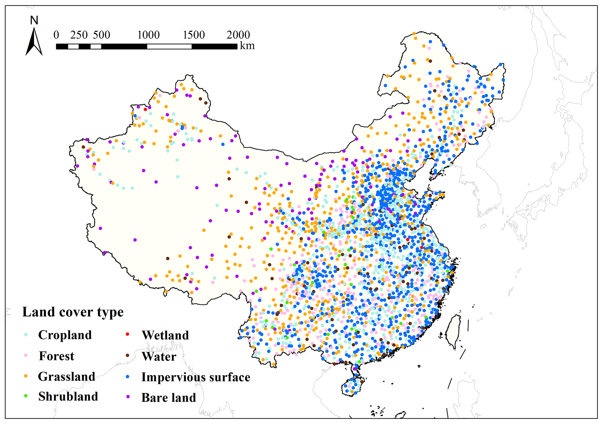
Figure 1 Study area and the location of meteorological stations used in this study. Each dot represents a station, and different colors correspond to different land cover types as shown in this figure legend.

2.2 Remotely sensed data

The satellite datasets used in this study are listed in Table 1.

Table 1 The satellite datasets used in this study.

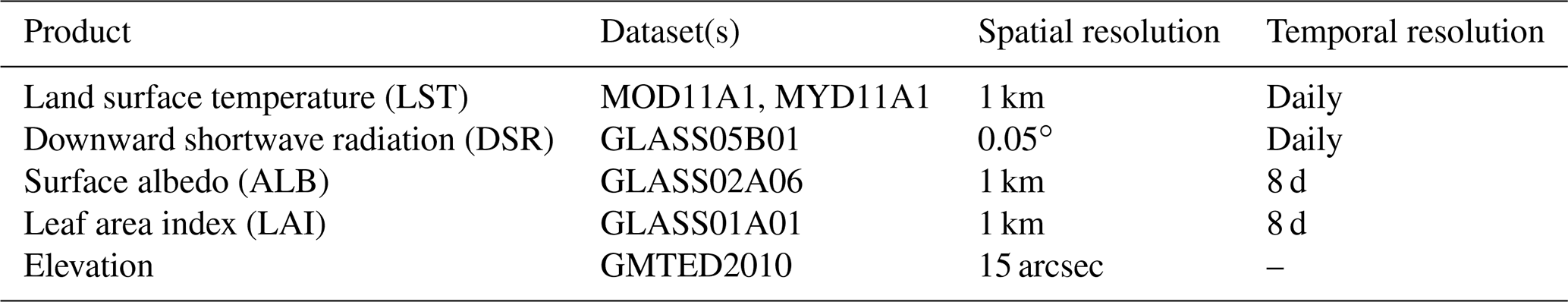
Terra and Aqua MODIS daily 1 km LST products (MOD11A1/MYD11A1, C6) both provide daytime and nighttime LSTs with a spatial resolution of 1 km (Wan et al., 2015).

Three all-sky products from the Global LAnd Surface Satellite (GLASS) products suite (Liang et al., 2013, 2021) were used, including the GLASS 1 km 8 d surface broadband albedo (ALB) product GLASS02A06 (Liu et al., 2013), the GLASS 0.05^∘ daily downward shortwave radiation (DSR) product GLASS05B01 (Zhang et al., 2019), and the GLASS 1 km 8 d leaf area index (LAI) product GLASS01A01 (Xiao et al., 2014). For the ALB product, we used the black-sky albedo of shortwave (BSA_sw), visible (BSA_vis), and near-infrared (BSA_nir) bands. As radiation products, DSR and ALB determine the shortwave solar radiation received at the surface and the fraction of total radiation reflected and absorbed by the surface, respectively.

The Global Multi-resolution Terrain Elevation Data 2010 (GMTED2010) elevation dataset, downloaded from the United States Geological Survey (USGS, https://topotools.cr.usgs.gov/GMTED_viewer/viewer.htm, last access: 24 August 2021), was also chosen to estimate T_a.

3 Methods

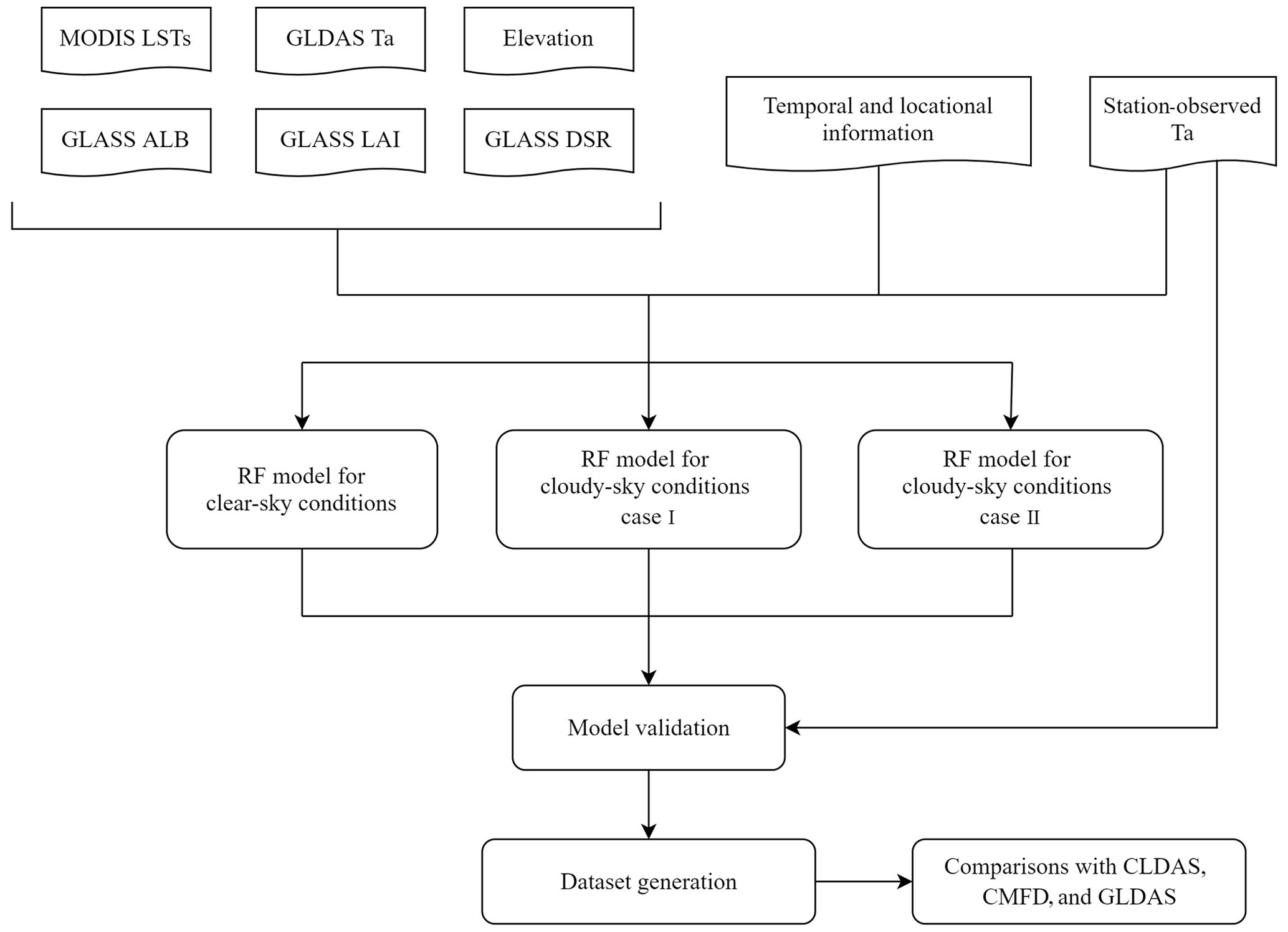
The overall framework of this study is shown in Fig. 2. First, all datasets from 2003 to 2019 were preprocessed into identical spatial and temporal resolutions. Second, we filled the gaps of MODIS LSTs and then divided all data pairs into three weather conditions according to the gap-filling results. Next, the values of all datasets were extracted using the nearest-neighbor method according to the geographical location of stations and then matched with the in situ T_a to obtain data pairs. Data pairs under different weather conditions from 2003 to 2016 were randomly divided into training, validation, and test sets (ratio of $\mathrm{3}:\mathrm{1}:\mathrm{1}$). Three RF models for different weather conditions were established and trained using the training set. Three model validation strategies of random sample validation, leave-time-out (LTO) cross-validation (CV), and leave-location-out (LLO) CV were then used to evaluate the models. Finally, we used the models to develop the all-sky T_a dataset from 2003 to 2009 and compared it with the existing datasets.

Figure 2 The overall framework of this study.

3.1 Data preprocessing

Because the spatial and temporal resolutions of all datasets were not completely consistent, we preprocessed all remotely sensed datasets and reanalysis datasets from 2003 to 2019 into identical 1 km and daily spatial and temporal resolutions, respectively. DSR, elevation, and assimilated T_a were resampled to a 1 km spatial resolution using the nearest-neighbor method. As LAI and ALB datasets both have an 8 d temporal resolution, we first combined them into a time series and then interpolated the time series using the linear interpolation method to obtain the daily datasets. For GLDAS assimilation data with a 3 h temporal resolution, we averaged all assimilated instantaneous T_a in a day to acquire the assimilated daily mean T_a for all days.

The values of all datasets were then extracted using the nearest-neighbor method according to the geographical locations of stations and matched with the in situ T_a to obtain data pairs. Next, we used a temporal gap-filling method to fill the MODIS LST gaps and divided all data pairs into three weather conditions according to the gap-filling results. The detailed gap-filling method and strategy for the division into weather condition categories is described in the Sect. 3.2. The data pairs with different weather conditions from 2003 to 2016 were then randomly divided into training, validation, and test sets (ratio of $\mathrm{3}:\mathrm{1}:\mathrm{1}$). Among them, the training set was used for model training, the validation set was used to determine the best model parameters, and the test set was used to evaluate the final model performance.

3.2 Strategies for LST gap-filling and division into weather condition categories

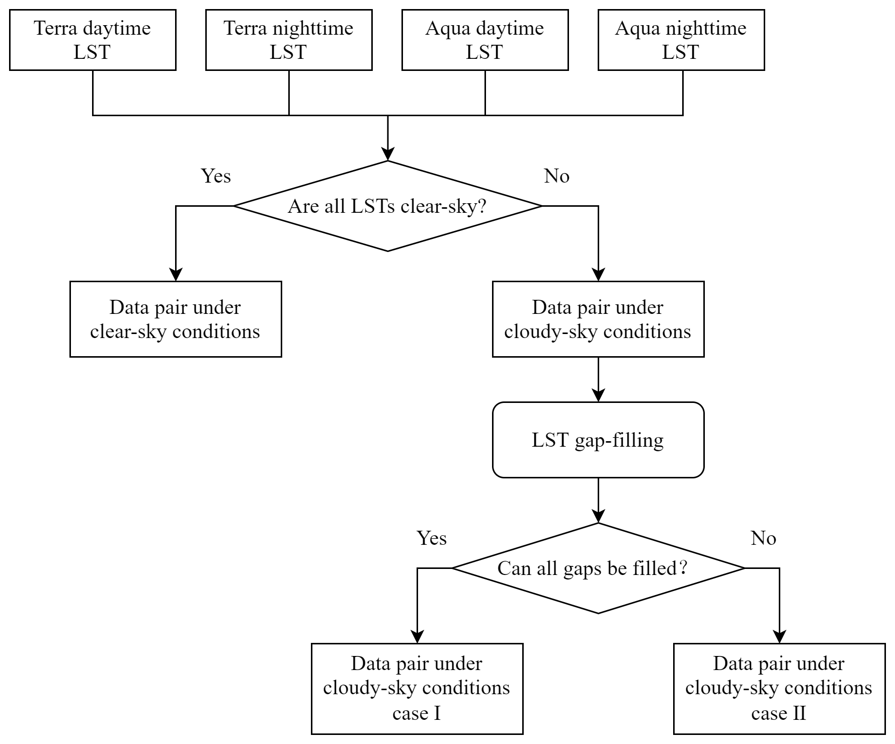
MODIS LSTs were produced under strict quality control, with each pixel marked as either a clear-sky or cloudy-sky observation. Pixels under cloudy-sky conditions had missing LST values, meaning that the LST-based method could not be applied to estimate T_a. In this study, a simple multitemporal method was used to fill the MODIS LST gaps. First, we set a time threshold (±2 d), and the missing pixel value was replaced by the clear-sky value of the nearest date within the set time threshold. If no clear-sky pixel was found within the time threshold, the missing pixel was not filled to avoid introducing high uncertainty caused by a huge temperature change between dates with large differences. This multitemporal method was used to fill the gaps of all four MODIS LSTs each day.

Considering the differences in the relationship between T_a and other features under different weather conditions, we divided data pairs into clear-sky conditions and cloudy-sky conditions according to the LSTs gap-filling results. When all four LSTs in a day were under clear-sky conditions, the data pair was identified as being under clear-sky conditions; otherwise, it was identified as being under cloudy-sky conditions. To control the uncertainty introduced by LST gap-filling, cloudy-sky conditions were divided into two cases: case I and case II. In particular, a data pair was identified as being under cloudy-sky conditions case I when there were LST gaps in the data pair and the gaps could be filled using the method mentioned above. If the LST gaps could not all be filled, the data pair was identified as being under cloudy-sky conditions case II. Therefore, we finally divided all data pairs into three weather condition categories: (1) clear-sky conditions, (2) cloudy-sky conditions case I, and (3) cloudy-sky conditions case II. The detailed criteria for dividing weather conditions are shown in Fig. 3.

Figure 3 The criteria for the weather-condition-based division of a data pair.

Next, we established three machine learning models (clear-sky model, cloudy-sky model I, and cloudy-sky model II) and trained them separately for different weather conditions. Daily LSTs were used in models for clear-sky conditions (clear-sky model) and cloudy-sky conditions case I (cloudy-sky model I), but not for cloudy-sky conditions case II (cloudy-sky model II). GLDAS-assimilated T_a, GLASS DSR, GLASS ALB, GLASS LAI, elevation, and temporal and locational information were also used in all three models as input features. For the clear-sky model, the utilized features included four clear-sky LSTs in a day. The qualification for a pixel of a given day to be judged as clear-sky may be harsh, but this ensured the use of completely clear-sky LSTs. The features of cloudy-sky model I included gap-filled LST(s), which increased the availability of LST, but the simple gap-filling strategy also introduced errors to the models. To avoid instilling high uncertainty caused by a large temperature change between dates with large differences, cloudy-sky model II did not use LST to estimate T_a.

3.3 Random forest

The RF method (Breiman, 2001) is an ensemble learning method based on classification and regression tree (CART) proposed by Breiman et al. (1984). Since it was proposed, it has attracted the attention of quite a few fields of study and has specifically had various applications in remote sensing in recent years (Gislason et al., 2006; Ham et al., 2005; Li and Zha, 2019; Xu et al., 2014).

A decision tree is a tree-like prediction model composed of nodes and directed edges. In each internal node of the decision tree, the sample set is segmented by selecting the optimal splitting feature until the segmentation termination condition is reached. Each path from the root node to the leaf nodes of a decision tree forms a classification. There are many algorithms for decision tree, such as ID3 (Quinlan, 1986), C4.5 (Quinlan, 1992), and CART. These algorithms all adopt the top-down greedy algorithm, and each internal node chooses the feature with the best classification effect to split, in order to achieve the goal of dividing samples into subsets that are as homogenous as possible, with the fastest speed. In the generation algorithms of ID3 and C4.5 decision tree, information gain or the information gain rate is used as the criterion to judge the optimal segmentation. Another type of optimal segmentation criterion is Gini impurity, which is utilized in the CART decision tree. In the RF model, multiple CART decision trees are included. The bagging method (Breiman, 1996) is used to generate independent identically distributed training sample sets for each tree and train on them.

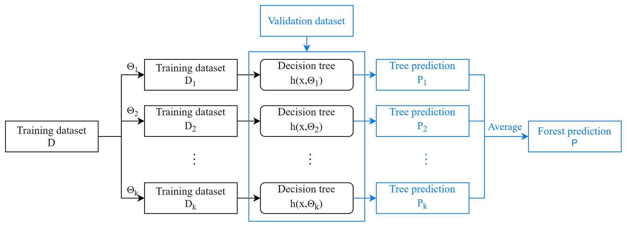
Although the application of RF at present is mainly focused on classification, it can be also used in regression analysis effectively, which can usually achieve higher accuracy than traditional regression analysis methods. The training and prediction process of the RF regression model is shown in Fig. 4. First, the bootstrapping method is used to acquire k datasets $\mathit{\{}{D}_k,k=\mathrm{1},\mathrm{2}\mathrm{\dots }\mathit{\}}$ and then k decision trees $\mathit{\left\{}h\right(x,{\mathrm{\Theta }}_k),k=\mathrm{1},\mathrm{2}\mathrm{\dots }\mathit{\}}$ are established, respectively, where x is the input vector, and Θ_k ($k=\mathrm{1},\mathrm{2}\mathrm{\dots }$) is the random vector determining the sampling of bootstrap datasets and candidate splitting features of each tree. The construction of a decision tree is realized by iteratively dividing the datasets into two subsets. Different from the RF classification model, the mean square error (MSE) is used as the optimal segmentation criterion in the RF regression model to split the nodes. Each decision tree in the RF regression model takes values rather than types as output targets, and the average of the predicted values of all the trees $\mathit{\left\{}h\right(x,{\mathrm{\Theta }}_k),k=\mathrm{1},\mathrm{2}\mathrm{\dots }\mathit{\}}$ is used as the final prediction.

Figure 4 The training and prediction process of the RF regression model.

3.4 Model training and validation

During the model training process, the training set was used for model training, and the validation set was used to determine the models with the optimal hyperparameters.

Compared with artificial neural network, the RF regression model does not need to carry out complicated parameter tuning work, and changing some insignificant parameters of the RF model may not cause substantial fluctuations in model performance. The two most critical hyperparameters, ntree and mtry, need to be determined during training. Among them, ntree refers to the number of decision trees in the RF model. Increasing ntree is conducive to improving the model performance and stability but also affects the computational efficiency of the program. Mtry refers to the maximum number of features used in a single decision tree. When mtry is less than the total number of features, the segmentation of a node is determined based on partial features that are randomly selected rather than all features. Increasing mtry allows nodes to consider more features when splitting but also reduces the diversity of individual trees, thereby increasing the risk of overfitting. Therefore, both parameters need to be properly balanced and selected, and we used the validation set to evaluate the model performance with different combinations of parameters to obtain the optimal hyperparameters.

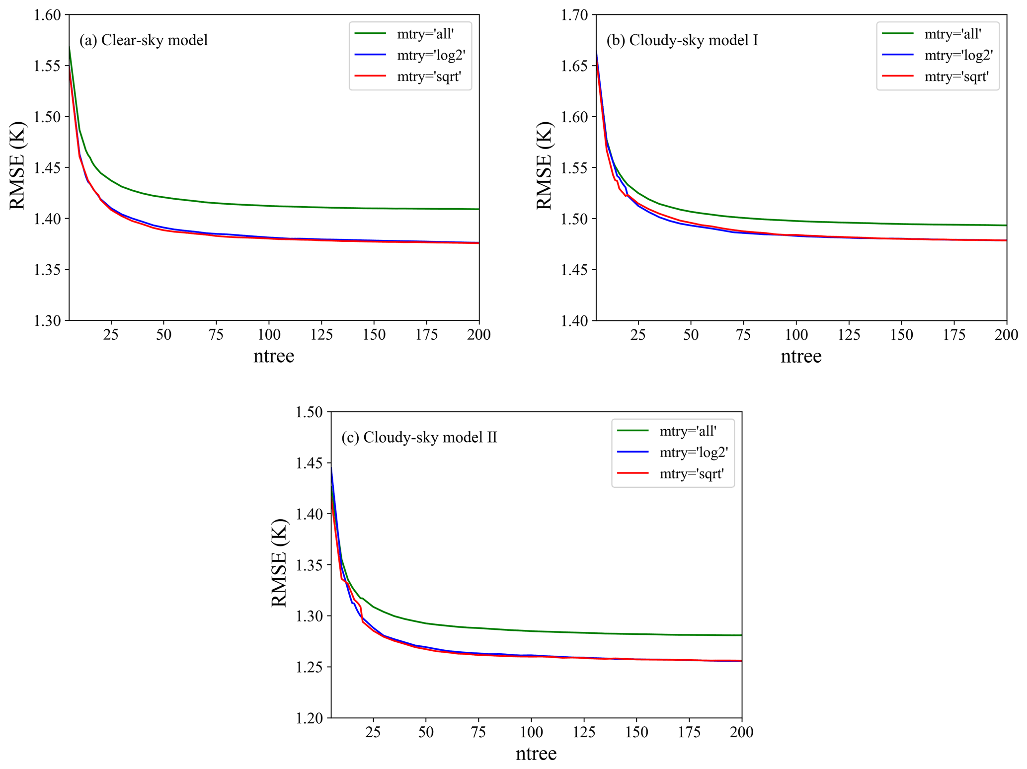
Assuming the total number of features of a sample is m, the values of mtry include log₂m, sqrt(m), and m, and ntree is set to 5–200. To analyze the RF model performance sensitivity to hyperparameters, the RMSE values of the three models for different weather conditions were calculated when setting different parameters, and the result is shown in Fig. 5. It can be seen from the results that with the change in model parameters, the three models showed similar variation patterns. With the increase of ntree, the RMSE value decreased gradually until it became almost constant (when ntree ≥ 100). The continued increase of ntree made very little contribution to improving the model performance but affected the computing efficiency. For mtry, we can see that using partial features (mtry of log₂m or sqrt(m)) resulted in significantly better performance than using all features (mtry of m). Overall, setting mtry to log₂m and sqrt(m) presented similar performance, and the setting of sqrt(m) performed slightly better than log₂m when ntree was larger than 175. Therefore, we set ntree to 200 and mtry to sqrt(m) in all models.

Figure 5 RF model performance sensitivity to hyperparameters.

To quantitatively evaluate the effect of each feature on the models, we calculated the feature importance (FI) of every feature using the permutation method for each model. The permutation method breaks the statistical relationship between feature i and the target variable and then measures the degree of deterioration in the model performance to evaluate the importance of feature i to the model (Mcgovern et al., 2019). Specifically, the model is first trained with the training set, and the RMSE of the validation set (RMSE_true) is then calculated using Eq. (1). For the calculation of the FI of feature i, RMSE_i is calculated again after all the features i of the validation set are shuffled. The difference between RMSE_true and RMSE_i is calculated and then divided by RMSE_true, and the result is used as FI, as shown in the Eq. (2). A large FI value means that the model performance decreases significantly after shuffling this feature, which indicates that this feature has a great impact on the accuracy of prediction results. On the contrary, if the model performance does not deteriorate significantly, it is obvious that this feature has less influence on the prediction process, or that other linearly dependent features are included in the model to make this feature redundant.

$$\begin{array}{}\text{(1)}& {\displaystyle }& {\displaystyle }\text{RMSE}=\sqrt{{\displaystyle \frac{\sum _{i=\mathrm{1}}^n{\left(y_{\mathrm{pre}}-y_{\mathrm{obs}}\right)}^{\mathrm{2}}}{n}}},\text{(2)}& {\displaystyle }& {\displaystyle }{\mathrm{FI}}_i={\displaystyle \frac{{\mathrm{RMSE}}_i-{\mathrm{RMSE}}_{\mathrm{true}}}{{\mathrm{RMSE}}_{\mathrm{true}}}},\end{array}$$

where y_pre refers to model prediction result, and y_obs refers to the corresponding station observation. RMSE_true is the RMSE of the validation set, and RMSE_i refers to the RMSE of the validation set after feature i has been shuffled.

The T_a predicted by the models was compared to the corresponding station observations. The RMSE, MAE, and R² were selected as criteria for model evaluation. In order to comprehensively evaluate the performance of the models, we adopted three model validation strategies: random sample validation, LTO CV, and LLO CV. For random sample validation, the test set (one-fifth of the total data from 2003 to 2016 selected randomly) was used to evaluate the performance of the final T_a estimation models. The results were grouped by elevation range, land cover type, and month to evaluate the model performance under different situations. For LTO CV and LLO CV, we divided all data pairs into 14 groups according to calendar year and 7 groups according to geographical location. In each iteration, one group of data was used for validation, and the other groups of data were used as the training set for model training. The modeling and validation process were repeated 14 and 7 times until each year's data and each cluster of data were validated, respectively. These two CV strategies have been used in some studies to evaluate the performance of spatiotemporal models in unknown time or unknown space (Liu et al., 2020; Ploton et al., 2020; Xiao et al., 2018).

4 Analysis of the results

4.1 Overall accuracy and model comparison

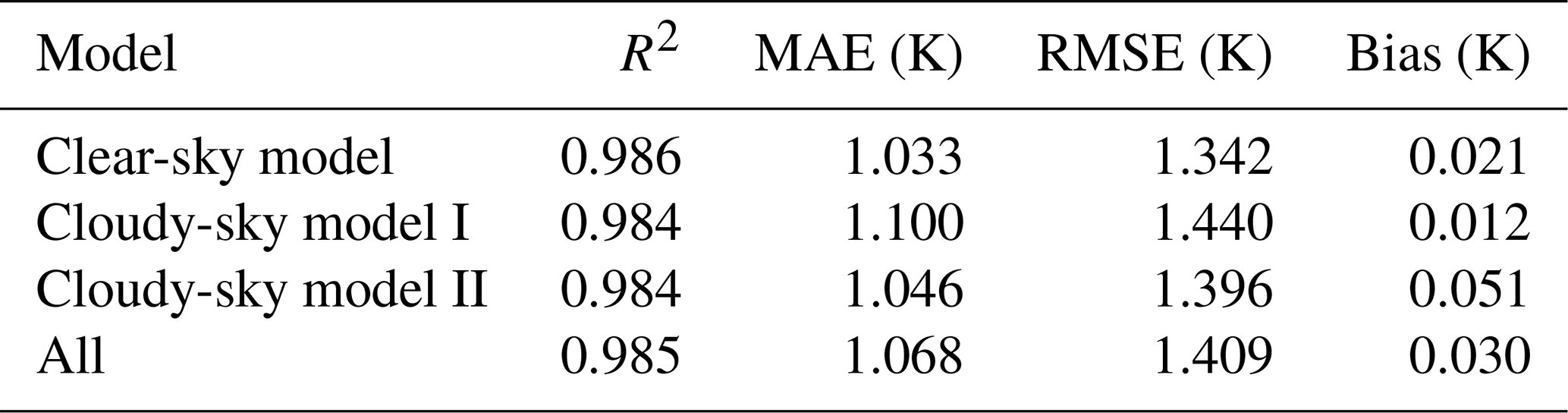
Approximately three-fifths and one-fifth of the data pairs from 2003 to 2016 were randomly selected for training and tuning the models, respectively, and the remaining one-fifth of the total data pairs were used to evaluate the performance of the final T_a estimation models. Validation statistics of models for different weather conditions and the overall accuracy of all estimated daily mean T_a are shown in Table 2. The three models presented similar validation statistics, with R², MAE, RMSE, and bias values ranging from 0.984 to 0.986, 1.033 K to 1.100 K, 1.342 K to 1.440 K, and 0.012 K to 0.051 K, respectively. The overall R², MAE, RMSE, and bias values of the estimated all-sky T_a were 0.985, 1.068 K, 1.409 K, and 0.03 K, respectively. Compared with the in situ T_a, the estimated T_a of all models showed a high correlation with little difference, confirming the great potential of the RF method to estimate the all-sky daily mean T_a over a wide spatial and temporal range.

Table 2 Model validation statistics.

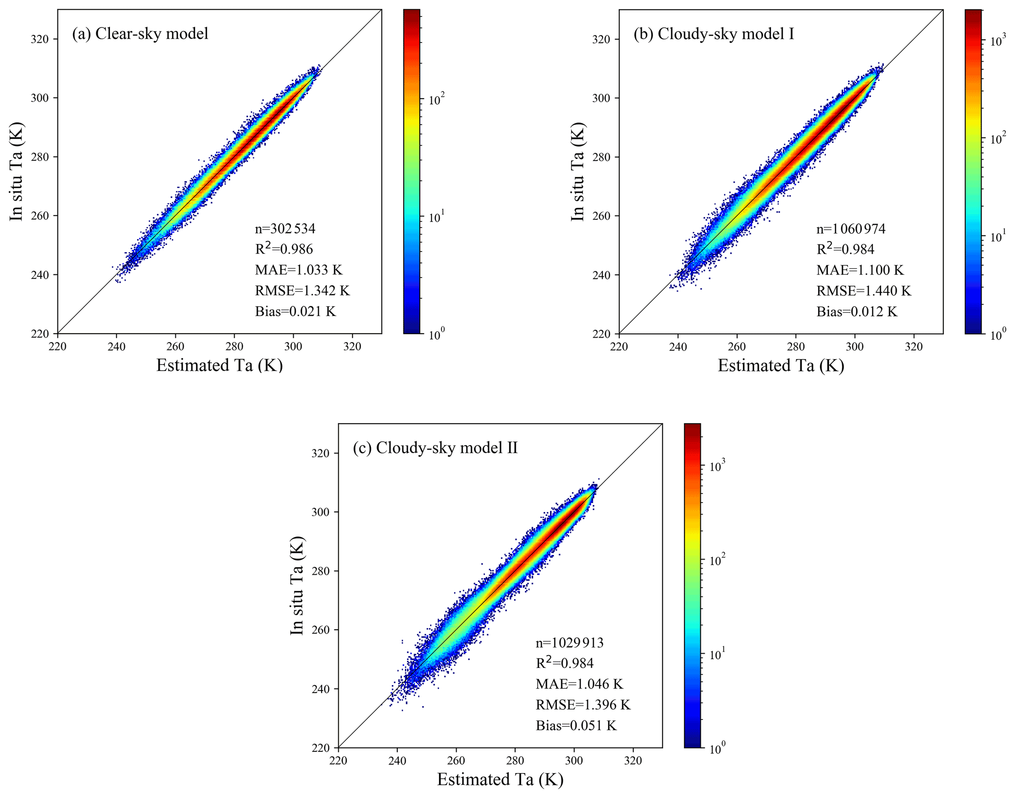
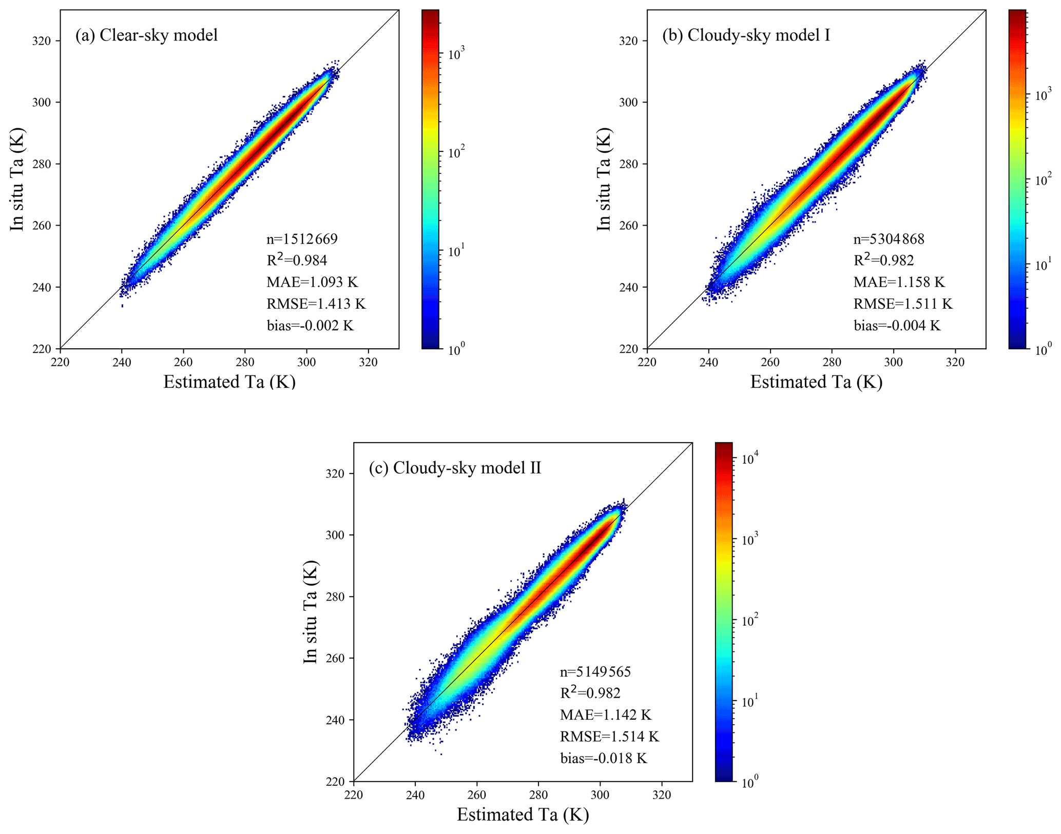
In addition, to further investigate the distribution of the prediction results and the differences between the three models, density scatterplots of the estimated T_a against the in situ T_a for the three models are shown in Fig. 6. In the three density scatterplots, most points were very concentrated near the 1:1 line, which also confirmed that these three models have achieved satisfactory accuracy in estimating daily mean T_a under different weather conditions. Among all the models, the clear-sky model had the highest stability and overall accuracy statistically, with the highest R² and the lowest MAE and RMSE. It could predict T_a under clear-sky conditions from less than 250 K to more than 300 K accurately and steadily. Compared with the clear-sky model, cloudy-sky model I had a relatively large error, which demonstrated that the LST gap-filling strategy adopted in this study introduced errors into the model to some extent, thereby increasing the uncertainty in estimating T_a under cloudy-sky conditions case I. The accuracy of the cloudy-sky model II was statistically similar to that of the clear-sky model, and it could predict a moderate temperature range close to 275 K with satisfactory performance. However, it can be seen from the density scatterplot for cloudy-sky model II that some discrete points deviated from the 1:1 line in the low-temperature range, which indicated that there may be much uncertainty in predicting the low-temperature range, especially at temperatures less than 260 K.

Figure 6 Density scatterplots of the estimated T_a against the in situ T_a for three models.

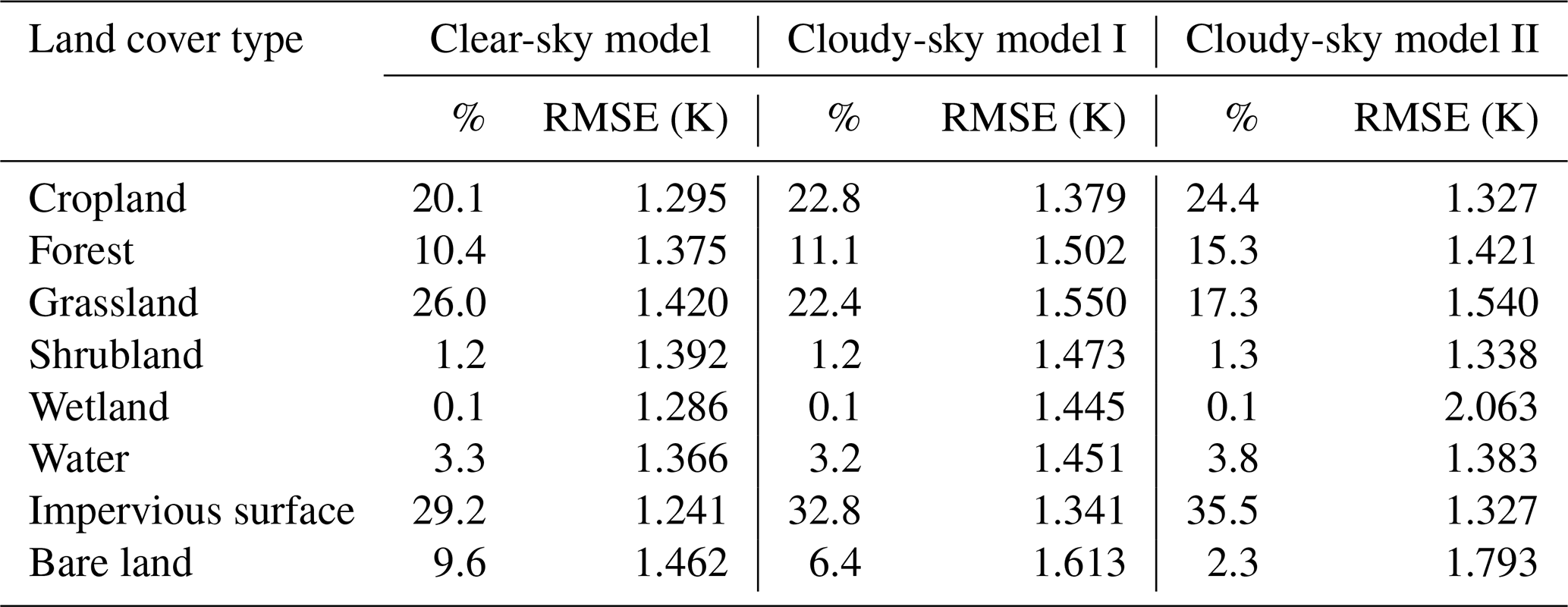
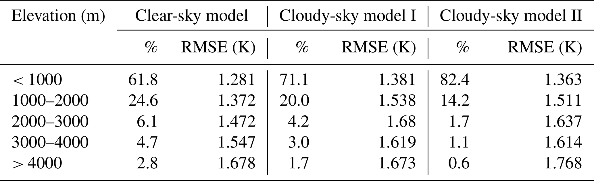
Many studies have proved that land cover type and elevation have a significant impact on the heterogeneity of T_a (Benali et al., 2012; Good et al., 2017; Lin et al., 2012; Marzban et al., 2017). Therefore, to comprehensively analyze the performance of the T_a estimation models, we grouped the results by land cover type and elevation range, and then compared the model performance for different groups. The model performance for different land cover types is listed in Table 3. All models showed relatively good performance (RMSE < 1.5 K) for cropland, shrubland, water, and impervious surface, whereas RMSE values were higher for grassland and bare land, which was consistent with the findings of Shen et al. (2020). The model performance for different elevation ranges is also listed in Table 4. With the increase in elevation, RMSE values of all models had a certain upward trend. However, as shown in the Fig. 7, the elevations of the stations used in this study are mainly distributed in the range from 0 to 2000 m, so the quantity of training samples in this elevation range have an absolute superiority, whereas the samples from higher elevations (elevation > 2000 m) only occupy a small part. The problem of class imbalance may contribute to the relatively large errors when predicting T_a at high elevation. In addition, factors such as complex and varied topography, vertical variation in T_a, and scale differences between remotely sensed image pixels and station observation data points will lead to high difficulty and uncertainty in T_a estimation at higher elevations (Rao et al., 2019).

Table 3 Model performance for different land cover types.

Figure 7 Elevation histogram of stations used in this study.

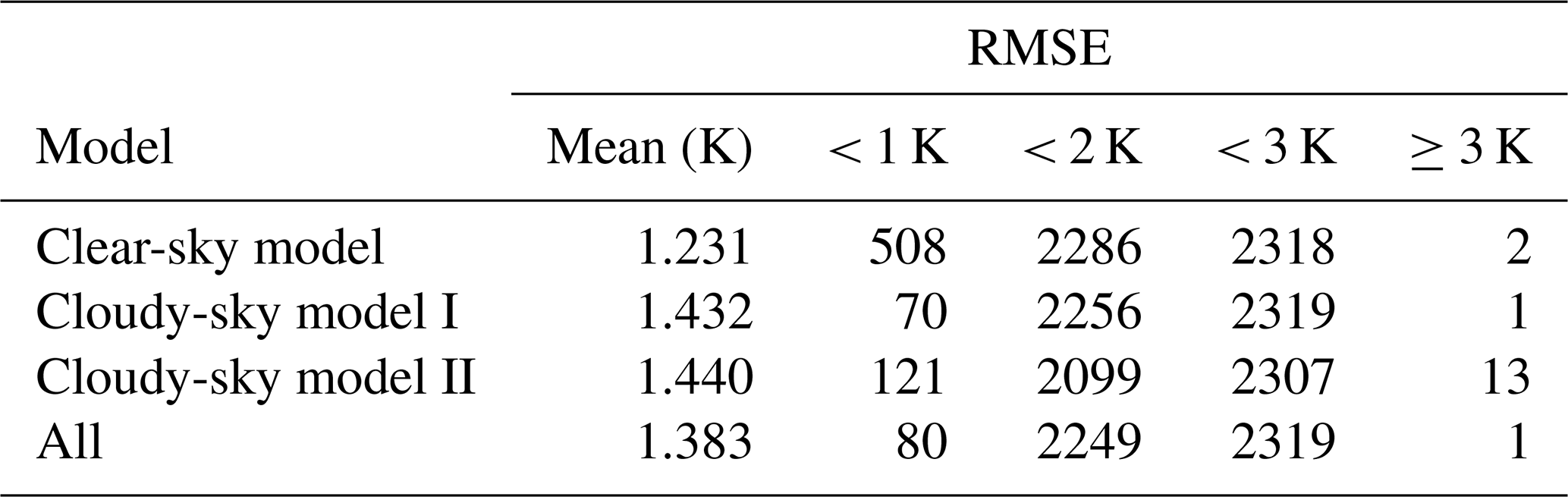
We further evaluated the error distribution of the three models at the stations. Due to the absence of in situ T_a at some ground stations on some days, only the stations that recorded more than 20 d for all three weather conditions were taken into account. Thus, the results of 2320 valid stations were finally obtained, as shown in Table 5. In general, the models showed good performance at most stations, with a mean RMSE value of 1.383 K. Moreover, 97 % of stations had RMSE values less than 2 K and only 1 of the 2320 statistical stations had an RMSE value greater than 3 K. The clear-sky model also had the best performance at the station scale, with the lowest mean RMSE of 1.231 K. A total of 508 stations had RMSE values less than 1 K, 2286 stations had RMSE values less than 2 K, while only 2 stations had RMSE values greater than 3 K. For cloudy-sky model I, the mean RMSE reached 1.432 K. The RMSE values of 2256 stations were less than 2 K, and only 1 station had an RMSE greater than 3 K. For cloudy-sky model II, the mean RMSE was 1.440 K, which was close to cloudy-sky model I, and 121 stations had RMSE values less than 1 K. However, 13 stations had RMSE values greater than 3 K for cloudy-sky model II, and most of these stations had RMSE values less than 3 K for the other two models.

Table 4 Model performance for different elevation ranges.

Table 5 Error distributions of three models at the stations.

For model comparison, as expected, the clear-sky model that used absolutely clear-sky LSTs performed better than cloudy-sky model I and cloudy-sky model II in almost every aspect and presented the highest stability. Cloudy-sky model I, which contained gap-filled LSTs, did not perform as well as the clear-sky model because, although the time threshold (±2 d) of the LST gap-filling method was relatively small, the LST value of a missing pixel of a date may be replaced by a clear-sky value with a difference of up to 2 d. However, the LST can vary considerably in just a few days, so the LST gap-filling process can introduce large errors into the model, thereby affecting the accuracy of T_a estimation. Surprisingly, cloudy-sky model II, which did not use LST features, achieved a comparative accuracy with the clear-sky model (respective RMSE values of 1.396 K vs. 1.342 K) statistically. However, when we further analyzed the model performance in specific situations, we detected differences in the performance of the three models. There may be considerable uncertainty associated with the cloudy-sky model II with respect to predicting the low-temperature range, especially at less than 260 K. Notably, cloudy-sky model II performed poorly for wetlands, with an RMSE of 2.063 K, whereas both the clear-sky model and cloudy-sky model I performed well on this type of land cover. This may be because wetlands are a mixture of water and land, with diverse complex ecological environments. Using LST can significantly improve the T_a estimation accuracy of this land cover type.

In summary, because of the strong correlation between T_a and LST, adding daily LSTs as features to models can improve the model stability and robustness. In the absence of LST, assimilated T_a can be used as a substitute for LST to provide an initial value or first guess for the model to estimate T_a with acceptable accuracy when combined with other features. However, the resolution of the reanalysis product is relatively coarse, and some local details were ignored when sampling from a larger scale (0.25^∘ × 0.25^∘) to a smaller scale (1 km × 1 km), thereby causing explicit uncertainties for cloudy-sky model II with respect to predicting the low-temperature range or some regions, especially some specific land cover types or regions with complex terrain. Overall, none of the three models showed significant differences in the model performance, and the model performance discrepancies for different land cover types and elevation ranges were acceptable. The proposed models can perform well in different situations and are suitable for T_a estimation under different weather conditions.

4.2 Cross-validation

In addition to random sample validation, two CV methods were used to further evaluate model performance. For the LTO CV, we divided the data pairs from 2003 to 2016 into 14 groups by calendar year. In each iteration, 13 groups of data were used as a training set for model training, and the remaining 1 group of data was used for validation. The modeling and validation process were repeated 14 times until the data for each year were validated. The results are shown in Fig. 8. The RMSE values of validation results for different groups of data ranged from 1.359 to 1.665 K. The minor difference between the LTO CV results proved that these models have good extensibility in time.

Figure 8 Density scatterplots of the LTO CV results for three models.

For the LLO CV, we then divided seven clusters in the Chinese region using the similar separation strategy of Xiao et al. (2018). Stations used in this study were divided into different clusters according to their spatial locations, and all data pairs were divided into seven groups according to the cluster of station. In each iteration, six groups of data were used as training sets and the remaining one group of data was used for validation. The modeling and validation process were repeated seven times until the data of each group were validated. The total validation results of the models under the three weather conditions are shown in Fig. 9, with RMSE values ranging from 1.615 to 1.957 K. As expected, the error of the LLO CV increased relative to random sample validation. This is because the relationship between T_a and other features varies with geographical location. The prediction error of the northwest and southwest clusters was larger than that of other clusters. The RMSE values of these two clusters exceeded 2.5 K under cloudy-sky conditions case II, whereas the RMSE values of the other clusters were about 1.5 K. This is consistent with the analysis of the spatial distribution of model accuracy in Sect. 4.4 of the paper. The meteorological stations in northwestern and southwestern China are distributed discretely and at a distance from other stations in China, leading to a large difference between the training set and the test set and, ultimately, resulting in the relatively poor performance in the LLO CV strategy in these two regions. Furthermore, the LLO CV results of cloudy-sky model II were worse than those of the clear-sky model and cloudy-sky model I, indicating that LSTs help to reduce the spatial overfitting of the models.

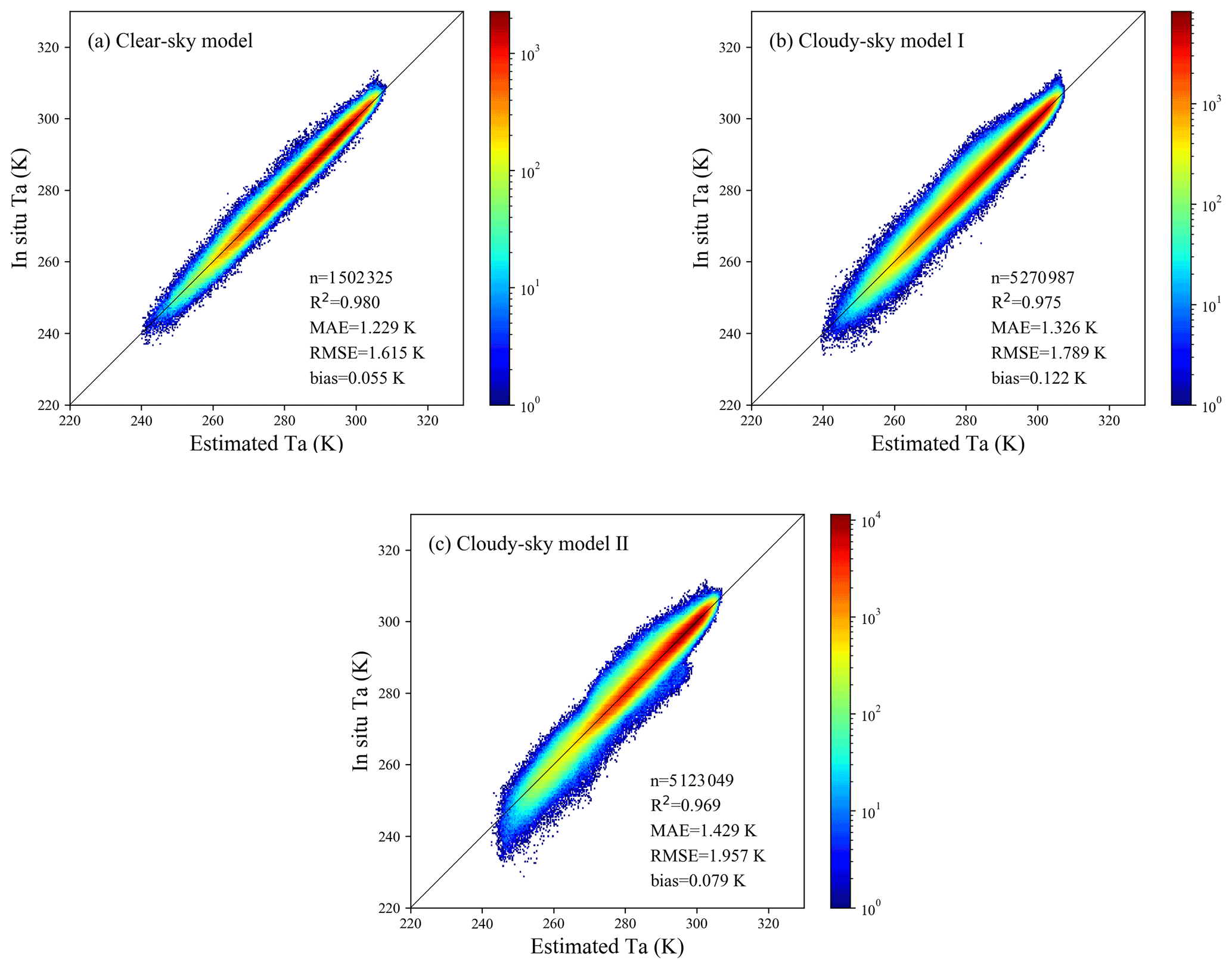
Figure 9 Density scatterplots of the LLO CV results for three models.

4.3 Feature importance analysis

To quantitatively evaluate the contribution of each feature included in the RF models, the FI of every feature for the three models was calculated using the permutation method described in Sect. 3.4 and was then ranked. To reduce the impact of contingency on the experimental results, we repeated the experiment 30 times and took the average value of all experimental results as the final FI of each feature for each model. The FI results are shown in Fig. 10, with the importance decreasing from top to bottom. The gray line indicates the FI range of each feature for multiple repeated experiments. All features are divided into four types and represented by different colors, among which the blue rectangles represent MODIS LSTs, the orange rectangles represent GLDAS-assimilated T_a, the red rectangles represent radiation products including DSR and ALB, and the green rectangles represent other features.

Figure 10 FI of each feature for three models.

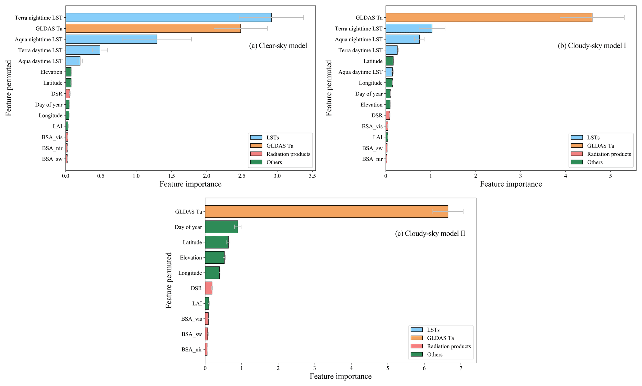
For clear-sky model, Terra nighttime LST was of the highest importance (FI of 2.92), followed by assimilated T_a (FI of 2.48), indicating that the prediction accuracy of the clear-sky model was significantly reduced after permuting these two features. They were followed by Aqua nighttime LST (FI of 1.3) and two daytime LSTs (FI of 0.49 and 0.21, respectively). For cloudy-sky model I, assimilated T_a ranked first (FI of 4.59), followed by Terra nighttime LST (FI of 1.03). For cloudy-sky model II, which did not include LST as features, assimilated T_a played a more importance role (FI of 6.65) than it did for cloudy-sky model I. The FI of radiation products and other features were all less than one for all the models, showing that they only slightly improved the model performance.

The energy exchange between the land surface and the near-surface atmosphere takes the form of longwave radiation, evapotranspiration, and turbulent exchange, or other phenomena. LST and land surface emissivity (LSE) determine the longwave radiation in land surface radiation and energy budgets (Liang and Wang, 2019). Thus, there is a strong and complicated physical correlation between LST and T_a. It can be seen from Fig. 8 that all four daily LSTs, especially nighttime LSTs, had relatively high FI values for both the clear-sky model and cloudy-sky model I. Among all the daily LSTs, nighttime LSTs outweighed daytime LSTs, and the Terra nighttime LST was of higher importance than the Aqua nighttime LST, which was consistent with the findings of many studies (Benali et al., 2012; Li and Zha, 2019; Zhang et al., 2011). In the study by Lin et al. (2012), the MAE between LST and T_a during the day and during the night were calculated separately, and they found that there was better agreement between LST and T_a during the night. In addition, due to the lack of solar radiation and its influence on the thermal infrared signal, remotely sensed nighttime LST products usually have higher stability (Benali et al., 2012; Vancutsem et al., 2010).

Assimilated T_a also mattered considerably for T_a estimation models. Its FI was second only to Terra nighttime LST for the clear-sky model and highest for cloudy-sky model I and cloudy-sky model II. For cloudy-sky model I, originally missed LSTs were replaced by clear-sky values from a nearby date, and the error introduced by this simple LST gap-filling strategy resulted in a decrease in the overall LST accuracy, thereby causing the FI of assimilated T_a to exceed that of LSTs. Compared with cloudy-sky model I, assimilated T_a was of higher importance, with a FI of 6.65 for cloudy-sky model II, indicating that it became the absolute dominant factor in T_a estimation when LST was not included in the T_a estimation model. Cloudy-sky model II also achieved satisfactory accuracy in the validation results. This demonstrates that although the spatial resolution of the assimilated T_a is relatively coarse, it can be a supplement or substitute for MODIS LSTs and provide an initial value or first guess for models to predict T_a with a higher resolution.

Radiation products and other features helped to improve the accuracy of T_a estimation models to a small extent. Among them, latitude, longitude, elevation, and day of year had relatively high importance in all three models. Latitude and longitude determine the relative position of the sun, which influences day length and, thus, the distribution of total solar radiation that the surface receives throughout the year; this, in turn, affects the patterns of T_a (Benali et al., 2012). Elevation affects how the ground is heated and how much radiation energy is absorbed by the atmosphere, resulting in vertical variations in T_a. In addition, the relationship between T_a and LST has great heterogeneity in different regions and at different times and is greatly affected by surface characteristics and atmospheric conditions. The day of year helps to explain the seasonal changes in atmospheric physical conditions, chemical composition, and surface characteristics to distinguish the different relationships between T_a and LST in different seasons and subsequently improve the accuracy of T_a estimation (Yao et al., 2020; Zhang et al., 2011). For LAI, DSR, and ALB, it is likely that other collinear features in the models made the information provided by them redundant, so their FI was relatively low in the T_a estimation models. However, in the analysis of the results of some stations, it was found that adding radiation features to the models helped improve the T_a estimation accuracy on some days. The radiation features can play a supplementary role in the case of some other features that do not perform well. Therefore, we finally decided to retain the radiation features in the T_a estimation models.

4.4 Spatial distribution of accuracy

The RMSE value was calculated for each meteorological station that recorded more than 20 d for all three weather conditions. To obtain a deeper understanding of the spatial distribution of model performance, the RMSE spatial distribution of stations for the three models was mapped, as shown in Fig. 11. It is evident that the model performance varied at different geographical locations for all three models. The clear-sky model presented the most stable results in different regions compared with cloudy-sky model I and cloudy-sky model II, with RMSE values of all stations ranging from 0.566 to 3.453 K. The RMSE range of cloudy-sky model I was 0.823–4.370 K and that of cloudy-sky model II was 0.809–4.198 K. The spatial patterns of cloudy-sky model I and cloudy-sky model II were generally similar, but there were more stations with good performance (RMSE < 1 K) and poor performance (RMSE > 3 K) for cloudy-sky model II, showing relatively poor stability.

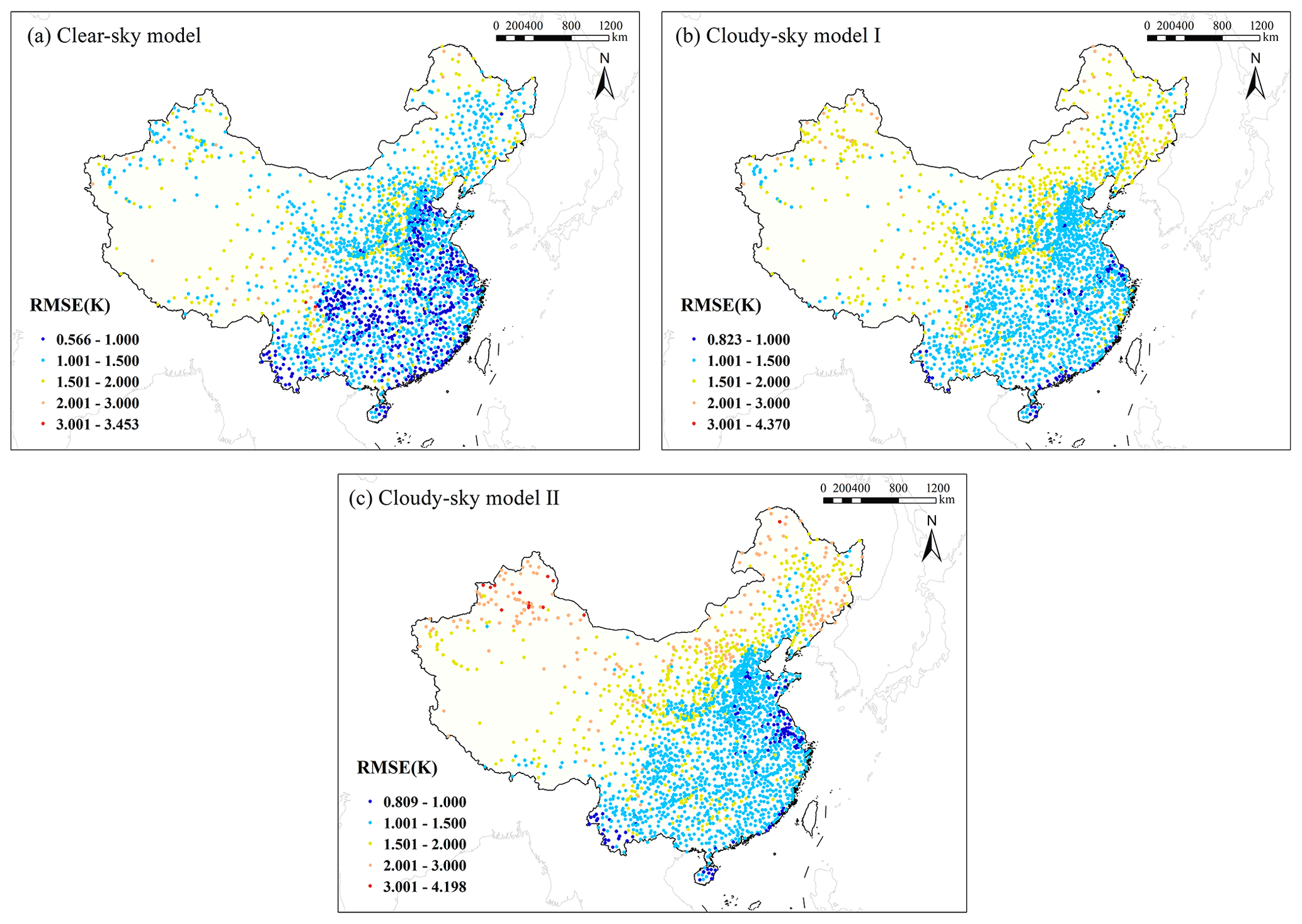
Figure 11 RMSE spatial distribution of stations for three models.

Overall, the stations in central, eastern, and southern China presented high levels of accuracy for all three models, with RMSE values of most stations in these places of less than 1.5 K. Most stations with large RMSE values were located in southwest, northwest, and northern China, which was consistent with the results of Shen et al. (2020), and the RMSE values of cloudy-sky model II in these positions were larger than those of the clear-sky model and cloudy-sky model I. On the one hand, the spatial heterogeneity of model performance is largely due to the uneven distribution density of meteorological stations. As can be seen from the geographical locations of the meteorological stations used in this study (Fig. 1), it is obvious that stations in central, eastern, and southern China are densely distributed, whereas stations in northern and western China are relatively rare, which may contribute to the uneven distribution of model performance. Additionally, the terrain environment in central, eastern, and southern China is not complex, whereas high elevation and some climate types will increase the uncertainty of T_a estimation in northern and western China. The climate types of stations with poor performance were mostly temperate continental and plateau mountain climates, and the land cover types were mainly bare land and grassland. It can be seen from Table 4 that cloudy-sky model II showed relatively poor performance for these two land cover types. Therefore, there was an explicit uncertainty when only assimilated T_a and other features except LSTs were included to predict T_a in places with these climate and land cover types. Overall, although the spatial distribution of the model performance was relatively uneven, the T_a estimation models for different weather conditions all showed satisfactory performance.

4.5 Seasonal distribution of accuracy

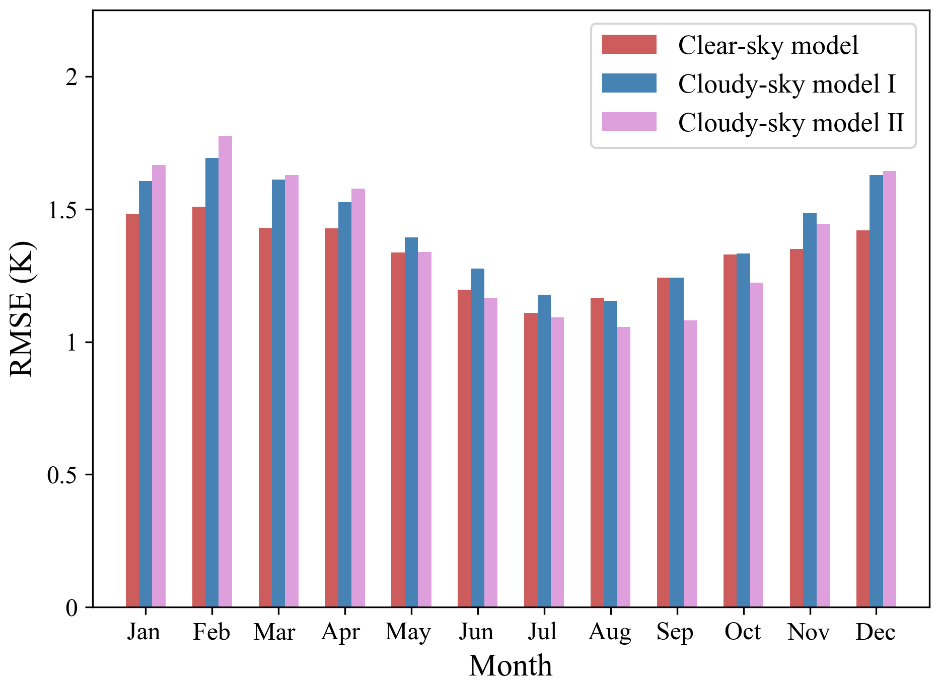
The model performance at the monthly scale was also evaluated, and the RMSE monthly distribution for the three models is shown in Fig. 12. The RMSE range of the clear-sky model was 1.109–1.508 K, the cloudy-sky model I was 1.178–1.692 K, and the cloudy-sky model II was 1.056–1.777 K. It is obvious that there was temporal heterogeneity in the model performance, and the estimation accuracy presented similar seasonal variation patterns for all three models. The RMSE values were lower in summer and autumn, and higher in spring and winter, reaching a peak in February and reaching a bottom in July or August. We can conclude that models performed better on warm days, with RMSE values for all three models of below 1.22 K in July and August. This finding was consistent with the validation results at the monthly scale of Yao et al. (2020) and Li and Zha (2019). This phenomenon may be partly due to the fact that China is vast in territory with a latitudinal difference between the northernmost station and the southernmost stations of about 30^∘; therefore, the range of T_a is wider on cold days than on hot days.

Figure 12 RMSE monthly distribution for three models.

Monthly differences in model performance also indicated that the relationship between T_a and other factors varied seasonally and may have been more consistent in the same month. It was confirmed in the research of Yao et al. (2020) that modeling data of the same month together could achieve more accurate results. Therefore, although day of year was used in the modeling in this study, this temporal difference was not completely eliminated. Modeling the datasets of all seasons together in this study may increase the temporal heterogeneity of accuracy. It is worthwhile considering grouping the data of the same month to establish monthly models in the future, which may be conducive to further improving the accuracy of T_a estimation.

5 Comparison with existing datasets

For a more comprehensive evaluation of the estimated daily mean T_a, we compared it with three reanalysis and meteorological forcing datasets, including CLDAS, CMFD, and GLDAS, in terms of validation statistics and spatiotemporal patterns. The station observations in 2010 were used to validate the accuracy of these four T_a datasets. It should be noted that we estimated daily mean T_a for the period ending at local midnight rather than 24:00 UTC. To ensure the time consistency, we calculated the average value of all simulations on a local day as the daily mean T_a for the reanalysis and meteorological forcing datasets. The statistical results and the density scatterplots are shown in Table 6 and Fig. 13, respectively. It can be seen that, compared with the reanalysis datasets, the RF T_a presented the highest consistency with the station observations, with the best performance in all accuracy assessment criteria (R², MAE, RMSE, and bias values were 0.992, 0.680 K, 1.010 K, and 0.063 K, respectively). The points in the density scatterplot of the RF T_a were more concentrated near the 1:1 line. CLDAS T_a and CMFD T_a both showed almost zero bias with the station observations, but their RMSE values were both close to 2 K. GLDAS T_a reported slight underestimation (bias of 0.900 K). In general, this comparison confirmed the applicability of the RF method in T_a estimation and the higher accuracy of our estimated T_a compared with the reanalysis products.

Table 6 Evaluation results of four datasets in 2010.

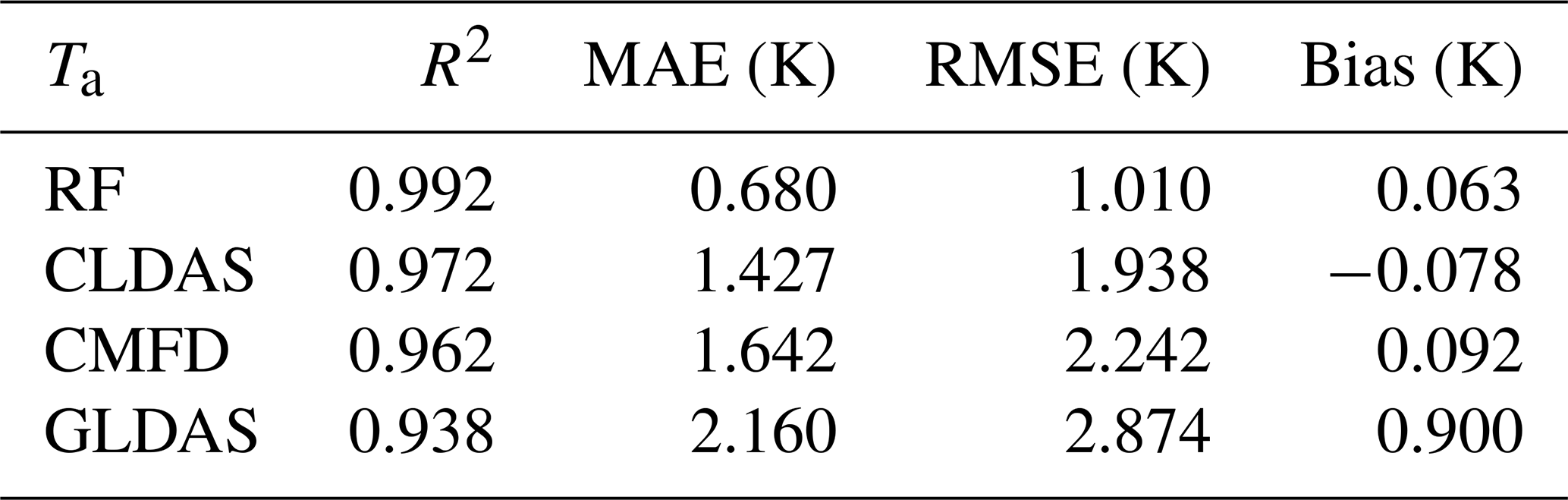
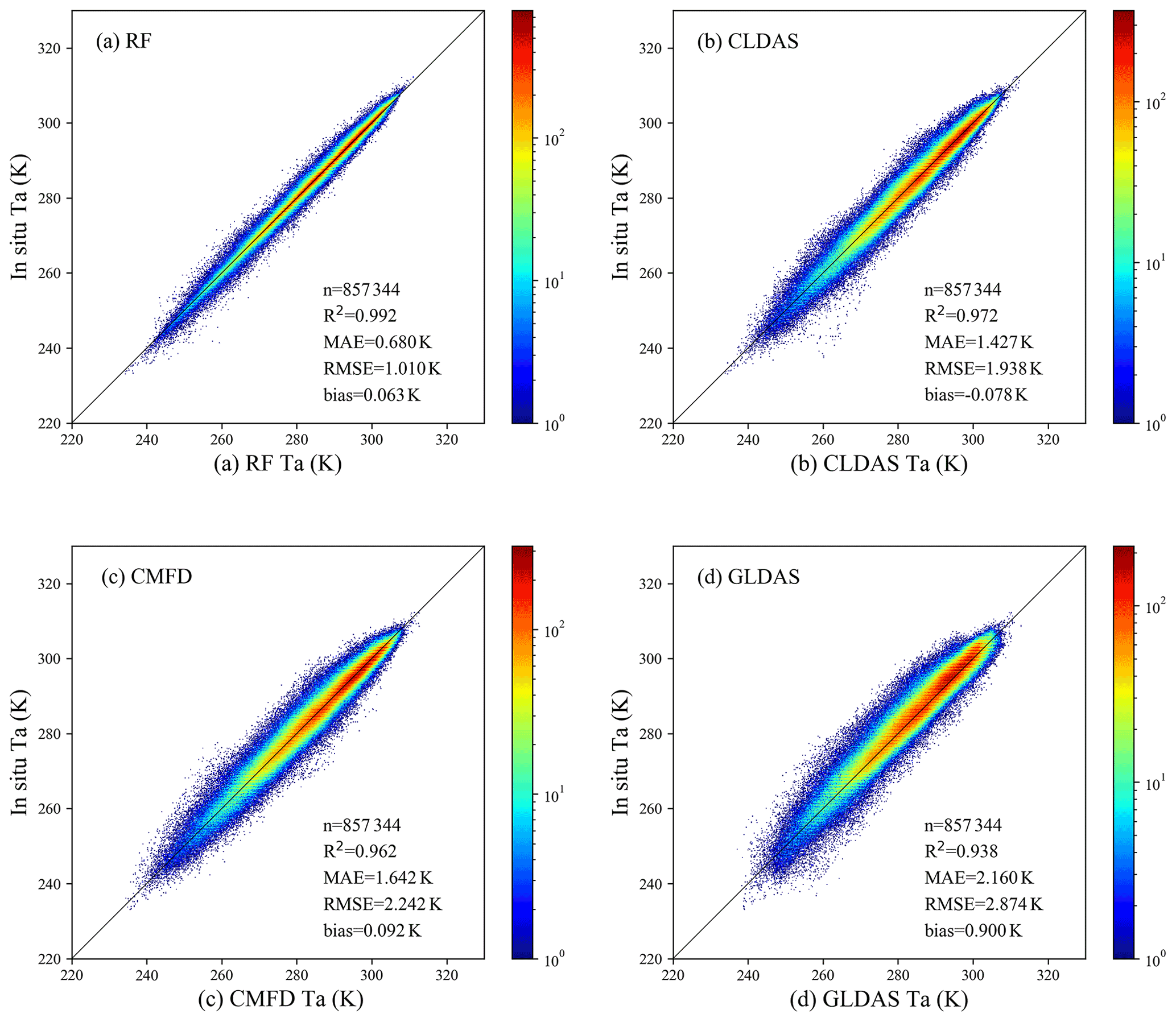
Figure 13 Density scatterplots of the estimated T_a and reanalysis T_a against the in situ T_a in 2010.

In addition, the spatiotemporal patterns of these four T_a datasets were compared. We calculated the monthly mean T_a in 2010 for all datasets. The RF monthly mean land T_a mappings over mainland China in February, May, August, and November 2010 are shown in Fig. 14a–d. The CLDAS (Fig. 14e–h), CMFD (Fig. 14i–l), and GLDAS (Fig. 14m–p) monthly mean T_a mappings in the same months are also shown in Fig. 12. The spatial resolutions of RF, CLDAS, CMFD, and GLDAS monthly mean T_a are approximately 0.01^∘ × 0.01^∘, 0.0625^∘ × 0.0625^∘, 0.1^∘ × 0.1^∘, and 0.25^∘ × 0.25^∘, respectively. We used GLDAS-assimilated T_a and GLASS LAI in T_a estimation, which have no value in most water bodies; thus, the T_a of these areas was also not estimated.

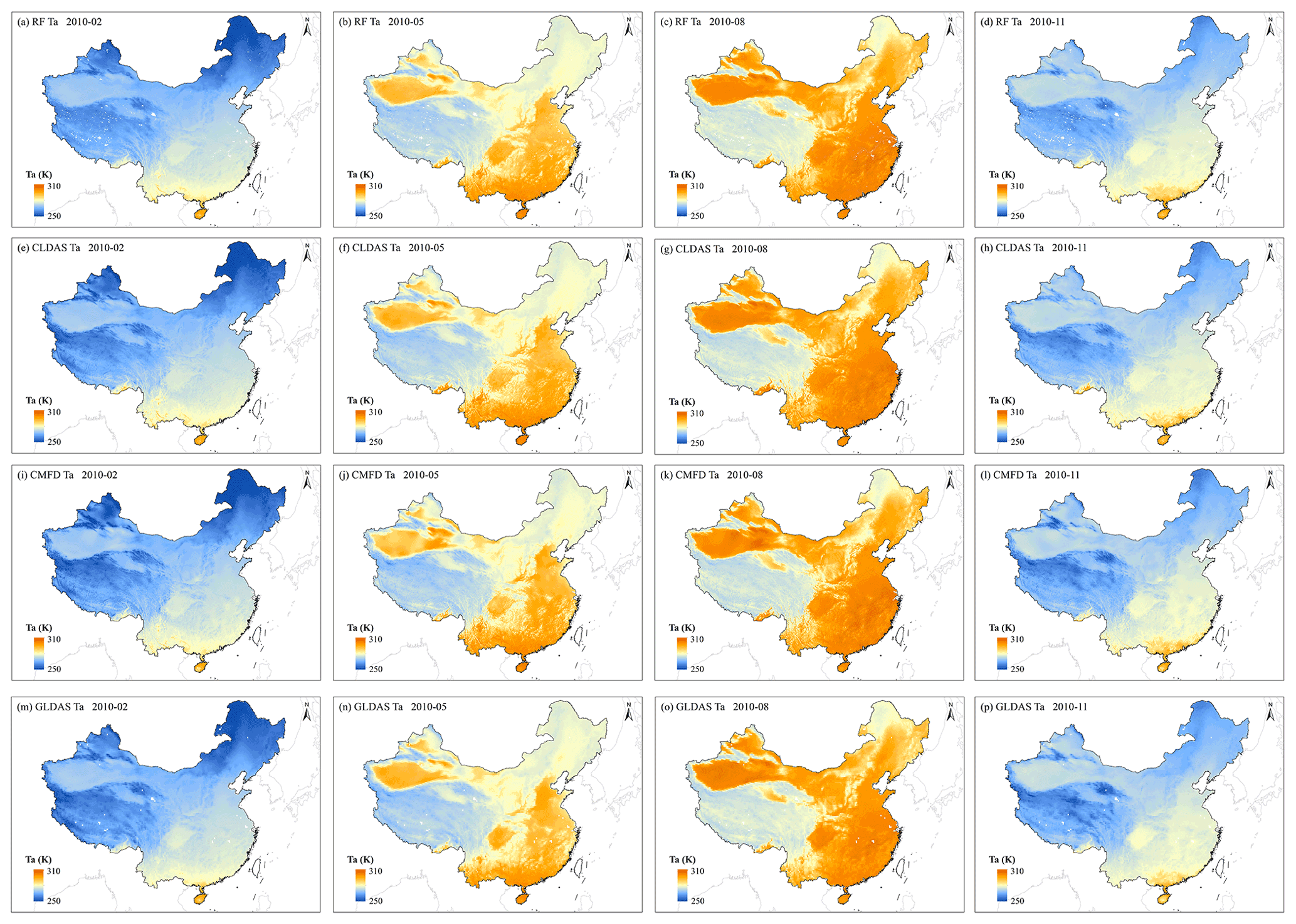
Figure 14 Maps of monthly mean T_a over mainland China. Panels (a)–(d) show the the RF T_a, panels (e)–(h) show the CLDAS T_a, panels (i)–(l) show the CMFD T_a, and panels (m)–(p) show the GLDAS T_a in February, May, August, and November 2010, respectively. The white pixels in mainland China indicate no data value and are always water bodies.

As can be seen from Fig. 14, it is clear that these four datasets basically showed a high degree of consistency in the spatiotemporal patterns over mainland China. China has a vast territory, and its topography is high in the west and low in the east. The spatial patterns of T_a over mainland China present great seasonal heterogeneity. In winter, the sun shines directly in the Southern Hemisphere, and the Northern Hemisphere consequentially receives less solar energy. The T_a in northern China and the Tibetan Plateau are generally low, and the T_a difference between the north and the south exceeds 50 K. On the contrary, in summer, as the sun shines directly in the Northern Hemisphere, T_a in most parts of China are generally high except for the Tibetan Plateau, with little T_a difference between the north and the south. As an expectable consequence of higher spatial resolution, the RF T_a mappings were capable of providing more detail on the T_a spatial patterns than the reanalysis and meteorological forcing T_a, especially in mountainous areas with complicated terrain. GLDAS T_a presented an obvious pixel effect because of the relatively coarse spatial resolution. In summary, the all-sky daily mean land T_a product developed in this study has achieved satisfactory accuracy and high spatial resolution simultaneously, which can reveal the seasonal variation trend and the spatial patterns of T_a over China well. This product can provide a long time series of daily mean T_a with the spatial resolution of 1 km over mainland China, which fills the current dataset gap in this field. Moreover, this product is also conducive to observing and analyzing the climate characteristic of China and plays an important role in the studies of climate change and the hydrological cycle.

6 Data availability

The daily mean land T_a product over mainland China is currently freely available at https://doi.org/10.5281/zenodo.4399453 for the period from 2003 to 2008 (Chen et al., 2021b) and at the University of Maryland (http://glass.umd.edu/Ta_China/, last access: 24 August 2021) for the period from 2003 to 2019. In order to make this big dataset easier to understand and use, we created a provincial sub-dataset with a smaller geographic coverage. An all-sky 0.01^∘ daily T_a product over Beijing (2003–2019) was generated from the developed dataset over mainland China after resampling and clipping, and it is publicly available at https://doi.org/10.5281/zenodo.4405123 (Chen et al., 2021a).

The MODIS product and the GLDAS dataset were downloaded from https://earthdata.nasa.gov/ (last access: 24 August 2021). The GLASS products were downloaded from http://www.glass.umd.edu (last access: 24 August 2021). The CLDAS and CMFD datasets were downloaded from http://tipex.data.cma.cn (last access: 24 August 2021) and http://data.tpdc.ac.cn/ (last access: 24 August 2021), respectively.

7 Conclusions

T_a is a key variable in climate and global change research. In this study, we developed an all-sky 1 km daily mean land T_a product for 2003–2019 over mainland China mainly based on MODIS and GLDAS data using the RF method. An efficient temporal gap-filling method was first used to fill MODIS LST gaps under cloudy-sky conditions. We predicted T_a under three different weather conditions separately: clear-sky conditions (when the daily LSTs are all clear-sky), cloudy-sky conditions case I (when the daily LST gap(s) can be filled), and cloudy-sky conditions case II (when the daily LST gap(s) cannot all be filled). The validation results using station measurements (one-fifth of the total data from 2003 to 2016 selected randomly), which were not used for model training, showed that the R² values were 0.986, 0.984, and 0.984 and the RMSE values were 1.342, 1.440, and 1.396 K for the clear-sky model, cloudy-sky model I, and cloudy-sky model II, respectively. In general, the models showed excellent performance at most stations, with a mean RMSE of 1.383 K, and there were 97 % stations with RMSE values less than 2 K and only 1 of 2320 stations with an RMSE value greater than 3 K. In addition, we examined the spatiotemporal patterns and land cover type dependences of model accuracy and concluded that model performance under all conditions was acceptable overall, despite some heterogeneity under different conditions. The relative contributions of different features to models were also quantitatively analyzed, and it was found that LST and assimilated T_a were of great significance in T_a estimation. Finally, we compared the T_a dataset in 2010 with the CLDAS, CMFD, and GLDAS datasets, finding great consistency in the spatiotemporal patterns. The estimated T_a in 2010 reported significantly higher accuracy against the station observations, with R², RMSE, and bias values of 0.992, 1.010 K, and 0.063 K, respectively.

Overall, this study developed a robust scheme that used a machine learning method to estimate all-sky daily mean T_a over a large spatial and temporal range. This approach can be applied globally. The generated all-sky T_a product has achieved a high degree of accuracy compared with the existing datasets, which fills the current dataset gap in this field and plays an important role in many scientific fields such as climate change, the hydrological cycle, and the energy balance. Future work should focus on developing better LST gap-filling methods and experimenting with more advanced deep learning methods that take the spatial and temporal dependence of T_a into account.