A global eddy-collocated temperature and salinity profile dataset (v1.0): integrating multiplatform in situ observations with satellite-tracking mesoscale eddies

Mesoscale eddies are ubiquitous rotating water masses with horizontal scales of tens to hundreds of kilometers that play a key role in redistributing heat and salt throughout the global ocean. However, the lack of long-term observational records has limited systematic assessments of their thermohaline effects from regional to global scales. Here, we present a global eddy-collocated temperature and salinity profile dataset spanning 29 years (1993–2021), constructed by integrating multiplatform in situ hydrographic observations with satellite-derived mesoscale eddy tracking products. The dataset contains 5.46 million quality-controlled temperature–salinity profiles, each collocated with its nearest mesoscale eddy and is publicly available at https://doi.org/10.5281/zenodo.20607854 (He, 2026). The observations provide broad global coverage, with most 2° × 2° grid boxes containing more than 200 profiles, enabling statistically robust analyses of eddy-induced temperature and salinity anomalies. Validation against previously documented regional eddy signatures demonstrates that the dataset reliably captures characteristic temperature and salinity anomaly structures associated with eddies. Example applications demonstrate its utility for characterizing regional three-dimensional eddy thermohaline patterns, assessing global eddy effects on upper ocean stratification and subsurface temperature extremes, and providing an observational basis for estimating eddy-induced heat, salt, and water-mass transports. As a long-term observation-based eddy-collocated profile product, this dataset provides a valuable resource for studies of eddy impacts on ocean circulation, tracer redistribution, climate variability, and model evaluation.

1 Introduction

Mesoscale eddies, as rotating currents with horizontal scales of O(100 km) and lifespans of weeks to months, are one of the most energetic and ubiquitous features in the global ocean (Chelton et al., 2011b). These features occupy 25 %–30 % of the global ocean surface and account for 90 % of the total kinetic energy in the ocean (Chaigneau et al., 2009; Ferrari and Wunsch, 2009). Through vertical thermohaline displacements, horizontal rotational advection, and lateral trapping (Gaube et al., 2014; McGillicuddy, 2016), eddies generate pronounced temperature and salinity perturbations that can extend hundreds to even thousands of meters below the sea surface (Frenger et al., 2015; He et al., 2018; Sun et al., 2017), playing essential roles in modulating upper-ocean heat and water mass redistribution (Dong et al., 2014; Sun et al., 2019; Zhang et al., 2014), regional circulation (Jan et al., 2017; Jing et al., 2020; Schubert et al., 2021), biogeochemical environments (Amos et al., 2019; Arostegui et al., 2022; He et al., 2021; Omand et al., 2015), and marine animal behaviors (Arostegui et al., 2022; Braun et al., 2025, 2019). These impacts highlight the importance of characterizing the three-dimensional thermohaline structure of eddies and quantifying their contributions to regional-to-global heat and salt redistributions.

Although significant advances have been made, important gaps remain in our understanding of the vertical structure, regional variability, and cumulative effects of eddy-induced thermohaline anomalies. For example, the intensity and penetration depths of eddy-induced temperature and salinity anomalies vary substantially among ocean basins (Lin et al., 2015; Schütte et al., 2016; Yang et al., 2013; Zhang et al., 2018), reflecting differences in background stratification, eddy nonlinearity, life-cycle stage, and interactions with mean currents and topography (He et al., 2020; Liu et al., 2019; Moreau et al., 2017; Samelson et al., 2014). Quantifying eddy-driven temperature and salinity anomalies and the associated heat and freshwater transports thus require large-amount observations that are targeted to eddy fields.

The emergence of high-resolution satellite altimetry products and automated eddy tracking algorithms has revolutionized the study of mesoscale eddies over the past two decades (Chelton et al., 2011b, 2007; Dufau et al., 2016). Although individual eddies vary in shapes, eddy-centric composite analyses reveals that the mean sea-level anomalies of eddies in a relatively small region exhibit a coherent monopole structure (Gaube et al., 2013; He et al., 2017), indicating that eddies have a robust regional mean character (Zhang et al., 2013). By collocating altimetric eddy fields with other concurrent satellite observations, the composite analysis has been widely used to reveal regional mean eddy impacts on sea surface temperature (Lv et al., 2022; Ni et al., 2021; Zhan et al., 2023), salinity (Delcroix et al., 2019; Hasson et al., 2019; Trott et al., 2019), chlorophyll (Chelton et al., 2011a; Frenger et al., 2018; He et al., 2021), and air-sea fluxes (Frenger et al., 2013; Guo and Timmermans, 2024; Villas Bôas et al., 2015).

Concurrently, in situ observing systems, such as mooring arrays, Argo floats, and gliders, have expanded rapidly. The World Ocean Database (WOD) now have collected millions of historical available temperature and salinity profile observation data from these instruments and platforms (Mishonov et al., 2024; Riser et al., 2016), making regional to global eddy-profile collocation feasible. By combining Argo profiles or subsets of WOD data with satellite eddy observations, studies have revealed the vertical structure of eddy-driven thermohaline anomalies and the associated transports in many oceans such as the South China Sea (He et al., 2018; Sun et al., 2018), the Indian Ocean (de Marez et al., 2019; Gulakaram et al., 2020; Yang et al., 2015), the North Pacific (Dong et al., 2017; Sun et al., 2017; Xu et al., 2016), the Southern Ocean (Frenger et al., 2015; Laxenaire et al., 2019), the Agulhas retroflection region (Laxenaire et al., 2020; Wei and Wang, 2025), and globally (Dong et al., 2014; Sun et al., 2019). However, most of existing studies focus on specific regions, time periods, instrument types, or coarse statistic grids, limiting global comparability.

In 2024, Ioannou et al. (2024) developed a global eddy dataset (TOEddies) with nearly 3 million collocated Argo profile data spanning 2000–2023, favoring global-scale analyses of eddy-induced subsurface variability. Subsequently, Simoes-Sousa et al. (2026) expanded this framework by incorporating additional profile observations from other instruments including Conductivity–Temperature–Depth (CTD), expendable bathythermograph (XBT), autonomous pinniped bathythermograph (APB), and gliders, producing an eddy-collocated dataset based on 4.2 million profiles and the altimetry-derived META3.2 DT eddy product. However, the profiles were only classified according to whether they were located inside or outside eddies. The absence of information on the relative distance between profiles and eddy centers limits the reconstruction of the three-dimensional structure of eddy imprints and the characterization of how eddy impacts vary with distance from the eddy core.

Here we address this gap by constructing a global eddy-collocated temperature and salinity profile dataset that integrates the world's most extensively accumulated historical hydrographic profiles (5.46 million profiles from the WOD) with mesoscale eddies identified from satellite altimetry (Fig. 1). All profiles collected during the satellite altimetry period are matched to the nearest eddy realization, and the profile–eddy distance is normalized by the eddy radius to provide a consistent spatial framework for composite and process-oriented analyses. Validations against published data and studies are processed to check the reliability of the data in capturing regional eddy thermohaline structures. Example applications are also provided to demonstrate the dataset's utility for characterizing, e.g., regional and global eddy-induced thermohaline anomalies, mixed-layer perturbations, extreme temperature events, and eddy-driven transports. By integrating satellited-derived surface eddy signatures with in situ subsurface temperature and salinity observations, this unified dataset provides a reproducible foundation for quantifying regional mean three-dimensional thermohaline structure of mesoscale eddies and their impacts across the global ocean, which may also provide a valuable benchmark for high-resolution (eddy-resolved) model evaluation, ocean state estimation, and climate research.

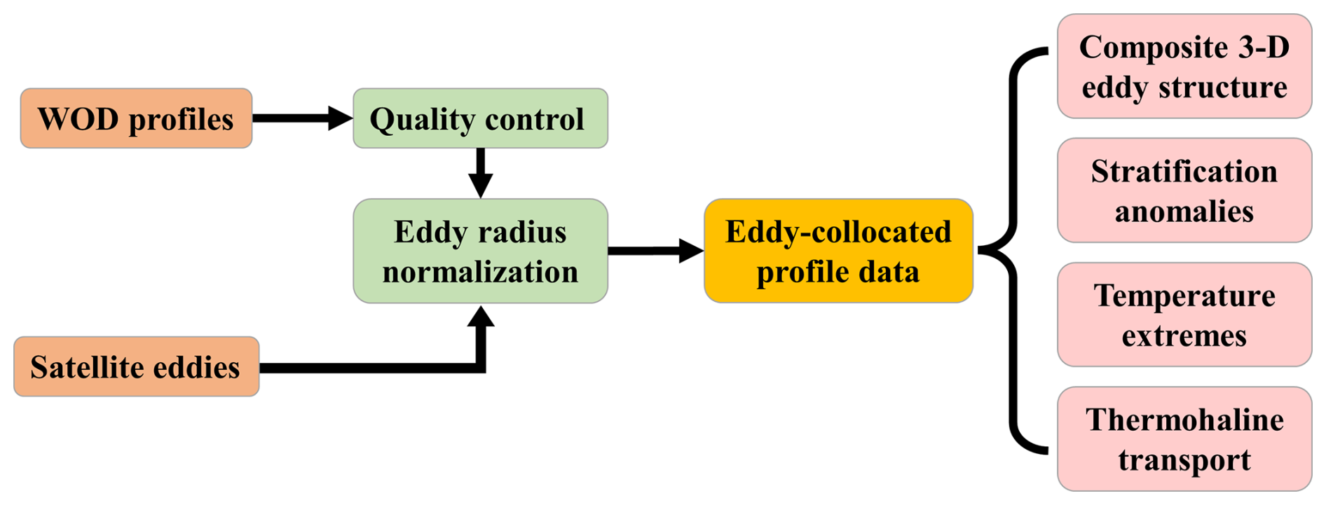
Figure 1 Flowchart illustrating the data source, main workflow, and potential implications of eddy-collocated profile dataset.

2 Data and methods

2.1 Mesoscale eddy product

Mesoscale eddies were identified and tracked based on overlapping closed contours of daily absolute dynamic topography (ADT) fields from multi-satellite altimeter data (Pegliasco et al., 2022). The global mesoscale eddy trajectory atlas product (META3.2, allsat) used in this study was produced by SSALTO/DUACS and distributed by AVISO⁺. The eddy product contains daily time series of the position, polarity (cyclonic/anticyclonic), amplitude, radius, rotational speed, and associated edge contours of each identified and tracked eddy trajectory between January 1993 and February 2022. Only those eddies with lifetimes longer than 10 d were considered have stable structures and used in this study.

In the Northern Hemisphere, eddies with regional extreme low (high) sea level anomalies and rotate anticlockwise (clockwise) are defined as cyclonic eddies (anticyclonic eddies). The vice versa in the Southern Hemisphere. Eddy radius is estimated as the radius of the best fit circle corresponding to the contour of maximum circum-average geostrophic speed at eddy edge (Pegliasco et al., 2022). Eddy amplitude is defined as the absolute SSH difference between the extremum sea level anomaly in eddy center and that at edge. Eddy rotational speed is estimated as the average geostrophic speed of the contour defining the speed radius. Eddy edge contour is the contour of maximum circum-average geostrophic speed for the detected eddy. A detailed description of the process of eddy detection, eddy tracking and the statistics of eddy outputs can be found in Pegliasco et al. (2022). To facilitate the analysis of eddy evolution, we added a normalized eddy age parameter by scaling the observation sequence number of each eddy trajectory to the range of 0 to 1. Based on eddy edge contours, we estimated eddy occurrence probability, at each $\mathrm{1}/\mathrm{4}$° × $\mathrm{1}/\mathrm{4}$° grid point, as the percentage of days a point is located within eddy interiors during the observation period.

2.2 Historical temperature and salinity profiles

The World Ocean Database (WOD) collected global historical available temperature and salinity profile measurements from a wide range of instruments and platforms, including ocean station data (OSD), CTD, XBT, APB, Argo float, moored buoy, drifter buoy, glider and others (Garcia et al., 2026; Mishonov et al., 2024). These profile measurements constitute the most comprehensive global in situ observation dataset, providing invaluable support for investigating ocean environment states and their changes under global warming. In this work, we used the quality-controlled and bias-corrected WOD temperature and salinity profile dataset (CODC-v2) developed by Zhang et al. (2024a) and Tan et al. (2025). This dataset not only applied systematic quality-control procedures to remove outliers, but also performed instrument-specific bias corrections, thereby retaining as many high-quality profiles as possible (Tan et al., 2023). From this product, we extracted approximately 5.46 million profiles collected between 1993 and 2021 that contain observations shallower than 20 m and deeper than 200 m.

To facilitate data usage, all extracted profiles were vertically interpolated onto a uniform depth grid extending from the surface to 1500 m, with vertical intervals of 5 m between 0–1000 m, 10 m between 1000–1500 m, and 50 m below 1500 m. This reduction in vertical grid resolution at depths aims to decrease storage requirements and computational memory usage. Considering that deep-ocean temperature variations are weaker and smoother than those near the surface, this adjustment may not substantially affect the statistical characteristics of eddy impacts (Dong et al., 2017; Frenger et al., 2015).

2.3 Collocating profile observations to eddy fields

To collocate in situ profile measurements to mesoscale eddies, we assumed that a given profile is influenced primarily by the eddy closest to its sampling location. For each profile, we searched for the nearest eddy, either cyclonic or anticyclonic, within a 10° × 10° grid box centered on the profile location on the same sampling day, and collocated the two accordingly. As eddies vary in size and shape, the distance between each profile and the center of its collocated eddy (d) was normalized by dividing it by the distance from the eddy center to the eddy boundary along the same azimuthal direction as the profile (D) (Fig. 2). This normalization transforms eddies of different sizes and shapes into a unified circular framework, facilitating intercomparison among eddies and enabling consistent dimensionless composite analyses of their thermal and biogeochemical imprints.

Figure 2 Schematic demonstrating the process of collocating WOD profiles to the nearest eddy and compositing them to a radius-normalized eddy‐centric coordinate. The circles are eddies of various sizes and the dots are data profiles. The d denotes the distance between a profile and its collocated eddy center, D represents the distance from the eddy center to the eddy boundary along the same azimuthal direction as the profile, and R is eddy radius.

This profile-collocating approach differs from methods that search for profiles around each eddy snapshot (Chaigneau et al., 2011; Sun et al., 2017; Yang et al., 2015). Considering that satellite altimetry typically resolves many more eddies than the ocean is sampled by in situ profilers (especially before 2010), associating each profile with its nearest eddy is computationally more efficient and avoids double counting. It prevents a single profile from being simultaneously assigned to both the interior of one eddy and the periphery of another, an ambiguity that commonly arises in “eddy-surrounding-search” methods when eddies are densely clustered.

2.4 Eddy imprints extraction

As most of the profiles were discretely sampled around or within different locations of different eddies, we cannot obtain the three-dimensional structure of a specific eddy. Whereas, within a relatively small region with relatively uniform thermal and dynamical environments, eddies are expected to share some common characteristics (Zhang et al., 2024b). Thus, we can reveal the mean eddy imprints by compositing eddy-associated profile observations to a uniform radius-normalized eddy-centric coordinate system based on their relative distance and azimuthal direction to eddy centers (Fig. 3). To remove seasonal cycle signals and diminish aliasing due to sparse historical sampling, temperature/salinity anomalies were estimated for each profile by subtracting the corresponding climatological monthly mean value at the nearest grid point in the World Ocean Atlas 2023 products (WOA 2023) (Swart et al., 2018).

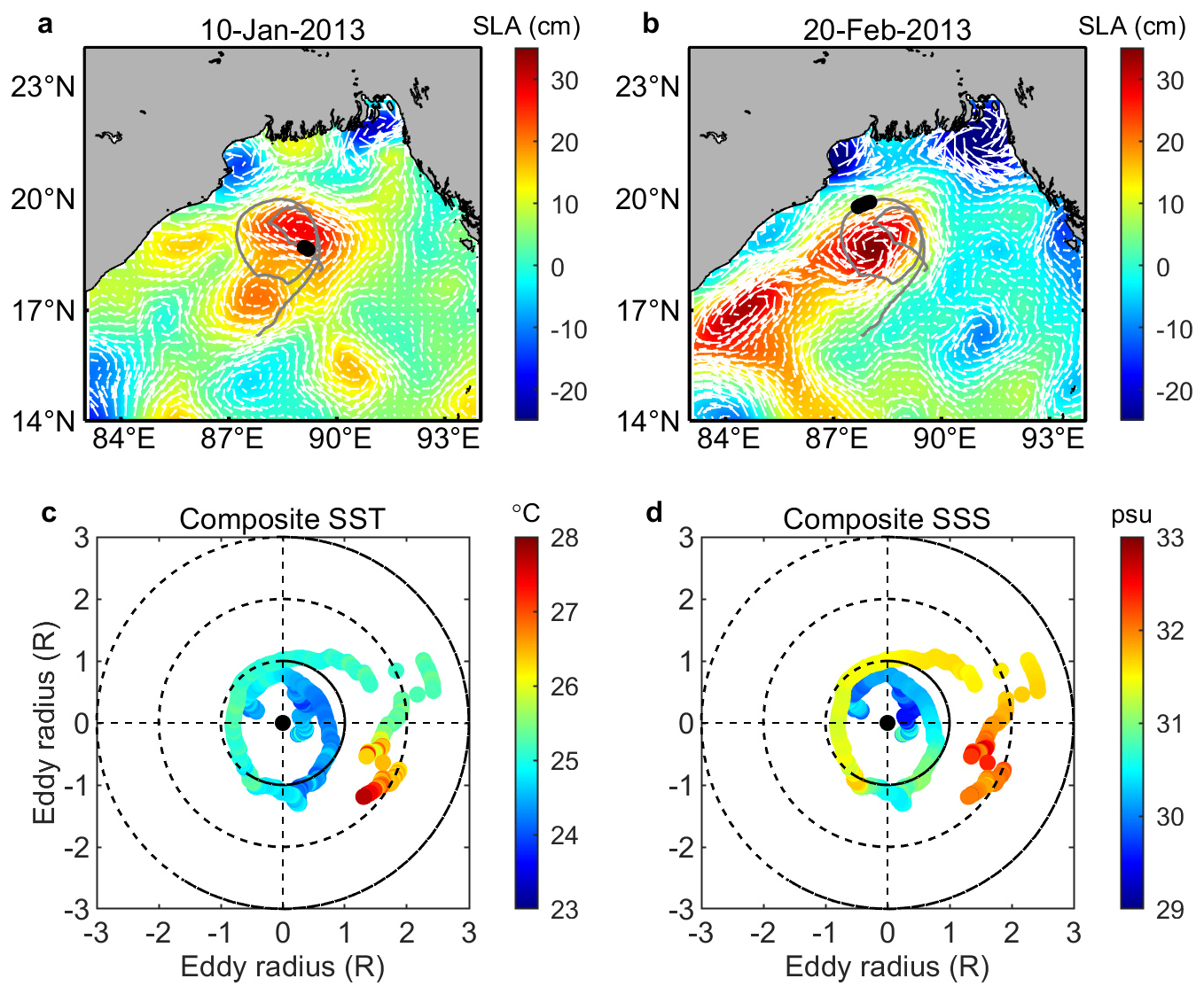
Figure 3 An example demonstrating the composite analysis of eddy effects on sea surface temperature and salinity using Argo float observations. (a–b) Geographic distributions of sea level anomalies (colors) and geographic current anomalies (vectors) in the Bay of Bengal on 10 January and 20 February 2013, respectively. The gray line indicates the trajectory of the Argo float (ID: 5903744) and the black dots are its positions at the sampling day. (c–d) Composite trajectories of the float relative to the center of the eddy. The colors are the float-estimated sea surface temperature (c) and sea surface salinity (d), respectively.

When all eddy-collocated profiles within a study region were mapped onto a normalized composite eddy framework, the scattered observations exhibit systematically higher/lower temperature and salinity values in eddy interiors relative to the eddy peripheries (Fig. 3c–d), highlighting the prevailing influence of mesoscale eddies on local thermohaline distributions. Then, by interpolating the scattered profile observations onto a standard three-dimensional grid, we can obtain the mean three-dimensional structure of eddy-induced temperature/salinity anomalies (He et al., 2018). Simultaneously, taking averages as a function of eddy radius can obtain the vertical section of temperature/salinity anomalies across eddy center. Mean temperature/salinity anomalies within eddies can be estimated by computing mean temperature/salinity anomalies between profile measurements within eddy interiors (d<1R) and outside eddies (usually d>2R) (He et al., 2024a). The choice of profiles outside twice eddy radii as referenced background fields aims to diminish the possible influence of twisted eddy shapes, vertical eddy tilting, and the complex submesoscale processes at eddy edges (Klein and Lapeyre, 2009; Li et al., 2022; Siegelman et al., 2019).

3 Results

3.1 Overview of the eddy-collocated profile dataset

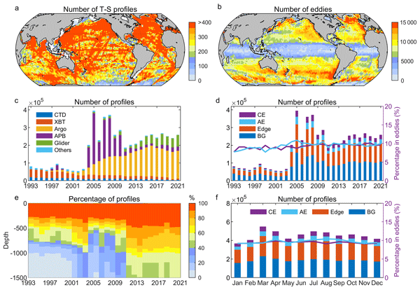
We obtained a total number of 5.46 million temperature and/or salinity profiles in the global ocean during the period with available satellite-derived eddy data (1993–2021) (Fig. 4). These profiles were collocated with cyclonic and anticyclonic eddy realizations, with 9.4 % and 9.7 % located within cyclonic and anticyclonic eddy interiors, respectively (Figs. 4d and 5). For each profile, the dataset provides the sampling time and location, vertical temperature and salinity distribution in the upper 1500 m, and corresponding temperature and salinity anomalies relative to the local monthly climatology (Table 1). In addition, the relative distance and azimuth between each profile and its associated eddy are provided. The dataset also includes key properties of the matched eddy, such as eddy center location, polarity (cyclonic/anticyclonic), amplitude, radius, rotational speed, edge contour, normalized age, and the trajectory number and observation number from the original eddy product (Pegliasco et al., 2022).

Table 1 Information of the eddy-collocated temperature and salinity profile dataset.

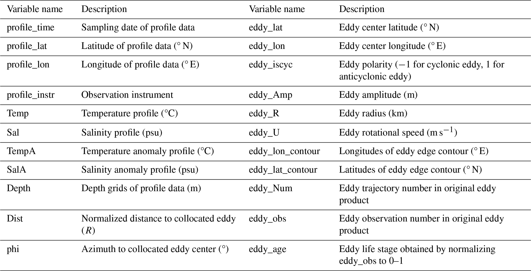
Figure 4 Spatial and temporal distributions of eddy-collocated temperature and salinity (T-S) profile data in the global ocean between 1993 and 2021. (a) Geographic distribution of the number of T-S profiles within 2° × 2° grid boxes. (b) The same as a but for the number of satellite-detected eddies. (c) Yearly statistics of T-S profiles from different instruments. (d) Yearly statistics of T-S profiles within cyclonic eddies (CE, d<R), anticyclonic eddies (AE, d<R), at eddy edges ($R<d<\mathrm{2}R$), and at background fields (BG, d>2R). The purple and cyan lines are the percentages of profiles within CEs and AEs, respectively. (e) The same as (c), but for the density of profile observations as a function of depth. (f) The same as (d), but for monthly statistics of the profile data.

The eddy-collocated profiles scattered across most regions of the global ocean, with the highest data density in the northwestern Pacific, the North Atlantic, and the northern Indian Ocean, where more than 400 profiles are available within a 2° × 2° grid box (Fig. 4a). Approximately 85 % of the statistical grid boxes between 60° S and 60° N has more than 200 profiles. Regions with relatively lower data density are primarily located in the South Atlantic and south of the Antarctic Circumpolar Current (ACC). Nevertheless, most of these regions still contain more than 100 profiles per 2° × 2° grid box, enabling the statistical analyses of eddy thermohaline imprints.

The number of the profile observations was relatively limited prior to 2003, averaging approximately 80 000 profiles per year (Fig. 4c). These profiles were derived mainly from ship-based CTD measurements and XBTs. Following the implementation of APB measurements, the number of profiles increased rapidly after 2004 and exceeded 200 000 per year. Although APB observations declined sharply after 2010 to less than 30 000 profiles annually, the increasing contributions from the Argo project and glider observations maintained the total number of profiles at a relatively stable level above 200 000 per year, substantially enriching the observational basis for investigating ocean environmental variability. Because profiles with maximum sampling depths shallower than 200 m were excluded, more than 90 % of the remained profiles in this dataset extend deeper than 300 m, over 80 % extend deeper than 500 m, and more than 60 % extend deeper than 1000 m (Fig. 4e). Profiles with relatively shallow sampling depths are mainly derived from CTD, XBT, and APB observations. In contrast, approximately 90 % of Argo profiles extend deeper than 500 m, and about 70 % reach depths greater than 1000 m (Mishonov et al., 2024).

Notably, the number of profiles included in this dataset is substantially larger than that used in our previous study (He et al., 2024b). One important reason is that profiles with relatively coarse vertical resolution were excluded in the earlier dataset. The profile number is also considerably greater than that in the dataset released by Ioannou et al. (2024) (∼ 3 million profiles) and Simoes-Sousa et al. (2026) (∼ 4 million profiles), primarily because the present profile dataset applies more comprehensive bias correction and quality re-control procedures to retain as many valid observations as possible (Zhang et al., 2024a). This substantial increase in profile number is particularly important for reconstructing regional mean three-dimensional eddy thermohaline structures and for investigating their seasonal and interannual variability.

Although the number of profiles exhibits pronounced interannual variability, the fraction of profiles located within mesoscale eddies remains relatively stable, with nearly 10 % occurring within cyclonic eddies and another 10 % within anticyclonic eddies, throughout the study period (Fig. 4d). Neither the total number of profiles nor the fraction of profiles located within eddies exhibits pronounced seasonal variability (Fig. 4f). Additionally, the proportion of profiles located within eddies closely resembles the geographic distribution of eddy occurrence probability (Fig. 5). These features suggest that the profile observations are approximately randomly sampled relative to mesoscale eddies. Therefore, the spatiotemporal inhomogeneity of the profile observations may not substantially bias analyses of eddy-induced temperature and salinity anomalies.

Figure 5 Consistency between the percentage of profile data within eddies and eddy occurrence probability. (a) Geographic distribution of the percentage of profile data within anticyclonic eddies (Γ_AE) within 2° × 2° grid boxes. (b) Geographic distribution of anticyclonic eddy occurrence probability (P_AE) estimated, at each $\mathrm{1}/\mathrm{4}$° × $\mathrm{1}/\mathrm{4}$° grid point, as the percentage of days a point was located within eddy interiors between 1993 and 2021. (c) Zonal averages of (a) and (b). (d–f) The same as (a)–(c), but for cyclonic eddies (CE).

3.2 Validation of the eddy-collocated profile dataset

To validate the capability of the eddy-collocated profile dataset in capturing eddy thermohaline structures, we first examined an eddy observation case that was tracked by an Argo float in the northern Bay of Bengal. The float was deployed southeast of an anticyclonic eddy at 89.5° E and 18° N on 2 January 2013 and then drifted within and around the eddy for more than one month (Fig. 3a–b). For each sampling day, the positions of the float were relocated relative to the eddy's center and mapped onto a radius-normalized eddy-centric coordinate. The resulting observations along the float trajectory show systematically lower sea surface temperature and salinity in the eddy interior compared to the surroundings (Fig. 3c–d), demonstrating that the eddy-centered composite framework is capable of revealing the thermohaline structure of the eddy.

Using the collocated profile dataset, we estimated mean eddy-induced temperature anomalies, within each 2° × 2° grid at representative depths of 20, 200, and 800 m across the global ocean, and compared the results with those derived from our previously dataset of He24 (He et al., 2024b) and the recently published dataset of Simoes-Sousa et al. (2026) (SS26) and Ioannou et al. (2024) (TOE). For each grid cell, the mean eddy-associated temperature anomaly was calculated as the difference between the average temperature anomaly inside eddies (<1R) and that outside eddies (>2R). The results reveal predominantly positive temperature anomalies within anticyclonic eddies and negative anomalies within cyclonic eddies in most regions of the global ocean, with the strongest signals occurring in the subsurface layers of midlatitude main current systems and subtropical gyres (Figs. 6 and 7). Both the horizontal distributions and vertical structures of the temperature anomalies closely resemble those derived from the He24, the SS26, and the TOE, yielding spatial correlation coefficients exceeding 0.8 at most of the analyzed depths (p<0.05).

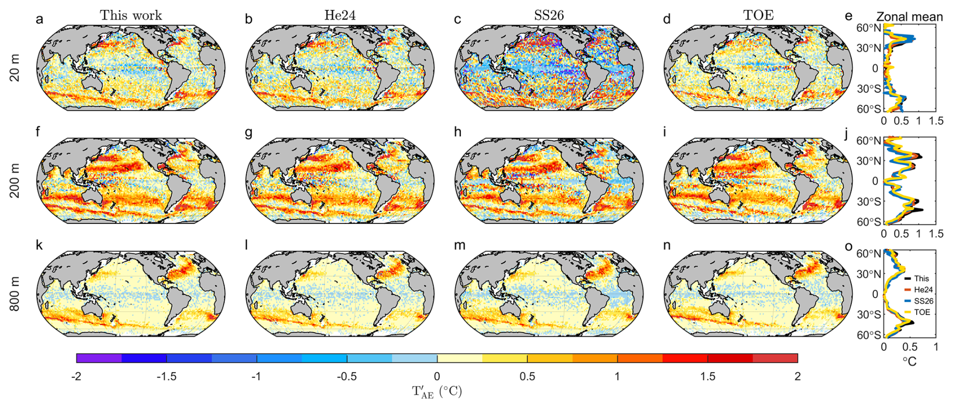
Figure 6 Geographic distribution of mean temperature anomalies within anticyclonic eddies, estimated within each 2° × 2° grid box, at the depths of (top to bottom) 20, 200, and 800 m. The left four panels are eddy-induced temperature anomalies estimated from the profile dataset in this study, He et al. (2024b) (He24), Simoes-Sousa et al. (2026) (SS26), and Ioannou et al. (2024) (TOE), respectively. The right panel is the zonal mean of the left four panels.

Figure 7 The same as Fig. 6, but for mean temperature anomalies within cyclonic eddies.

Notably, the temperature anomalies derived from the SS26 exhibit noticeably noisier patterns near the sea surface than those obtained from the other datasets (Figs. 8 and 9). A likely explanation is that their dataset excluded eddies with lifetimes shorter than 30 d or mean amplitudes smaller than 2.5 cm (Simoes-Sousa et al., 2026). Consequently, some profiles that would otherwise be associated with these weak eddies may instead be assigned to neighboring eddies, introducing additional uncertainty into the estimated temperature anomalies. Because the excluded eddies are generally weak and have relatively limited vertical influence, the impact of their exclusion is expected to decrease with depth, consistent with the reduced differences among the datasets in the subsurface ocean. Compared with TOE, the temperature anomalies derived from the present dataset are generally stronger in the midlatitude main current systems (Figs. 8 and 9). One possible explanation is that the TOE dataset detects a larger proportion of relatively weak eddies (Ioannou et al., 2024), resulting in weaker composite temperature anomalies after averaging.

Figure 8 Differences in mean temperature anomalies within anticyclonic eddies between this dataset and the other three datasets at 20, 200, and 800 m depths. The left three panels are the difference between this work and He24, SS26, and TOE, respectively. The right panel is the zonal mean of the left three panels.

Figure 9 The same as Fig. 8, but for temperature anomalies within cyclonic eddies.

Since approximately 80 % of the profile data used in He24 originated from Argo observations, the estimated eddy-induced temperature anomalies in that study can be regarded largely as Argo-based results. In the present study, a substantial number of observations from additional platforms were incorporated. Yet, the resulting temperature anomaly patterns remain highly consistent with the earlier results (Figs. 8 and 9). This agreement suggests that the inclusion of observations from multiple observing systems does not materially alter the statistical characteristics of the estimated eddy imprints. Rather, the improved quality control and expanded observational sampling are expected to reduce sampling-induced outliers in the estimated eddy-induced temperature anomalies, particularly in regions and time periods with sparse Argo observations, while enabling more robust analyses of mean eddy imprints at finer regional scales.

The temporal evolution of eddy-induced temperature anomalies is also highly consistent among the four datasets (Fig. 10). Overall, the SS26 dataset tends to produce slightly stronger near-surface temperature anomalies, whereas the TOE dataset generally yields weaker anomalies, consistent with the fact that SS26 excludes relatively weak eddies, while TOE identifies a larger proportion of weak eddies (Ioannou et al., 2024; Simoes-Sousa et al., 2026). These differences become much smaller in the subsurface ocean, where the four datasets exhibit remarkably similar temporal variability. More pronounced discrepancies occur prior to 2000, particularly in the Southern Ocean (the Agulhas System and the Brazil–Malvinas Confluence), where hydrographic observations were sparse before the Argo era. Consequently, the Argo-based TOE dataset exhibits large temporal fluctuations and substantial data gaps during the early years. By incorporating quality-controlled observations from multiple platforms, the present dataset provides a more temporally continuous record of eddy-induced temperature anomalies while remaining highly consistent with previous datasets. This improved temporal continuity extends the applicability of the dataset to investigations of seasonal-to-interannual variability and potential long-term changes in eddy-induced thermohaline anomalies.

Figure 10 Time series of eddy-induced temperature anomalies within anticyclonic and cyclonic eddies at depths of (top to bottom) 20, 200, and 800 m, estimated using a 12-month running mean. Columns correspond to the Kuroshio Extension (KE, 28–40° N and 140–180° E), the Gulf Stream (GS, 35–50° N and 30–70° W), the Agulhas System (AS, 27–42° S and 0–40° W), and the Brazil–Malvinas Confluence (BMC, 35–55° S and 30–65° W), respectively. Black, red, blue, and yellow curves represent estimates derived from the dataset developed in this study, He24, SS26, and TOE, respectively.

We further examined the spatial distribution of eddy-induced salinity anomalies. Unlike the relatively uniform sign of temperature anomalies (Figs. 6 and 7), salinity anomalies exhibit much more complex horizontal and vertical patterns (Figs. 11 and 12). In the near-surface ocean, salinity anomalies within anticyclonic eddies are generally positive in midlatitude main current regions but negative across much of the tropical and subtropical oceans (Fig. 11). At 200 m depth, however, positive anomalies become dominant within anticyclonic eddies across most regions. Cyclonic eddies exhibit broadly opposite anomaly patterns (Fig. 12). Despite the greater complexity of the salinity field, the spatial distributions derived from this dataset remain highly consistent with those obtained from the other three datasets (Figs. 11 and 12), confirming the robustness of the estimated eddy-induced salinity anomalies. For brevity, the differences in eddy-induced salinity anomalies among the datasets and their temporal evolution are not shown, as they generally resemble those obtained for temperature anomalies.

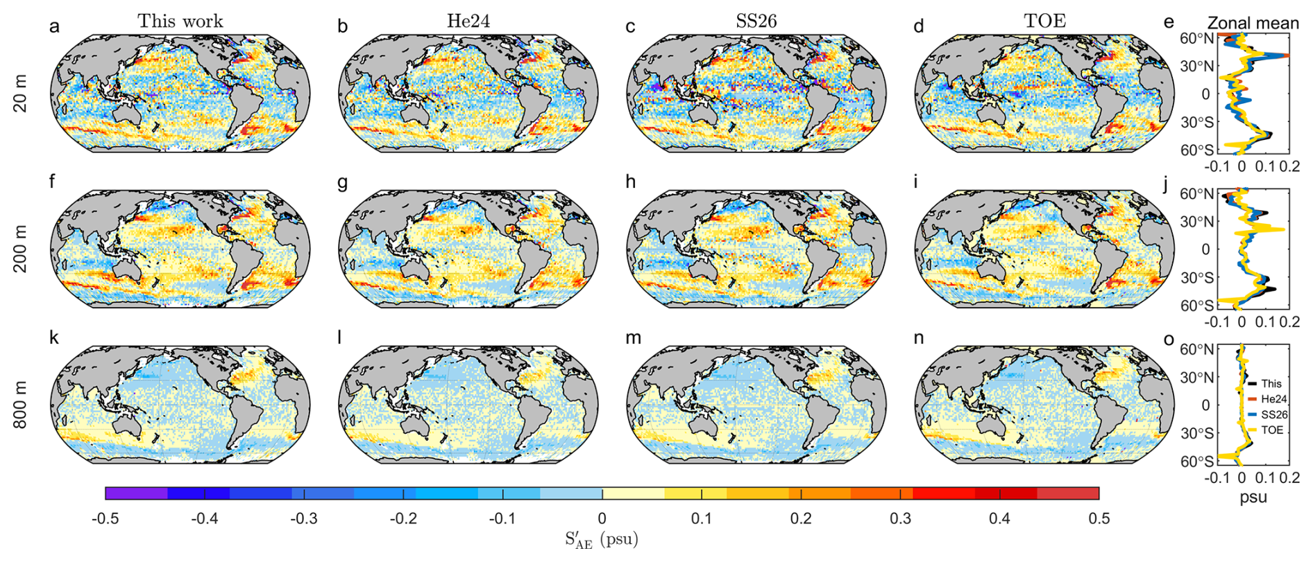
Figure 11 The same as Fig. 6, but for mean salinity anomalies within anticyclonic eddies.

Figure 12 The same as Fig. 7, but for mean salinity anomalies within cyclonic eddies.

We note that, despite the overall agreement among the datasets, isolated grid boxes with anomalously large temperature or salinity anomalies still occur in a small number of locations, particularly in equatorial regions where eddy activity is relatively weak. Such outliers appear less frequently in the present dataset and the He24. In the latter case, profiles with coarse vertical resolution were excluded, yielding a dataset dominated by Argo observations with relatively consistent sampling characteristics. For the present dataset, newly developed quality-control and bias-correction procedures were applied to identify and correct or remove anomalous measurements and problematic profiles (Zhang et al., 2024a). However, no automated quality-control system can completely eliminate all erroneous observations. Consequently, a small number of outliers remain. While their influence on basin-scale and global-scale analyses is negligible, additional screening may be beneficial for applications focused on limited geographic regions or individual eddy cases.

4 Potential data applications

4.1 Regional three-dimensional eddy structure

Compared with existing eddy-collocated products, the inclusion of relative distance and azimuthal direction of profiles to collocated eddy centers in this dataset enables the reconstruction of regional mean three-dimensional thermohaline structure of mesoscale eddies. As an example, we extracted all eddy-collocated profiles in the northern Bay of Bengal and mapped them onto normalized cyclonic and anticyclonic eddy-centric coordinate systems according to the polarity of their associated eddies (Fig. 13). The resulting profiles are relatively evenly distributed both within eddies and in the surrounding regions (Fig. 13b–c), providing sufficient sampling coverage for three-dimensional interpolation of temperature anomalies. The resulting composite fields reveal that the maximum negative temperature anomaly within cyclonic eddies occurs near the eddy center at a depth of approximately 110 m, with magnitudes exceeding 1.5 °C (Fig. 13d–e). The anomaly weakens progressively with depth and becomes negligible below 300 m. Anticyclonic eddies exhibit a similar vertical structure, but with positive temperature anomalies and a slightly deeper core depth of approximately 130 m. These features are in agreement with previously in situ eddy case studies in the Bay of Bengal (Sarma et al., 2018, 2020). Such three-dimensional representations provide a valuable basis for quantifying key eddy properties, including core intensity, spatial extent, penetration depth, and the associated heat and salt transports.

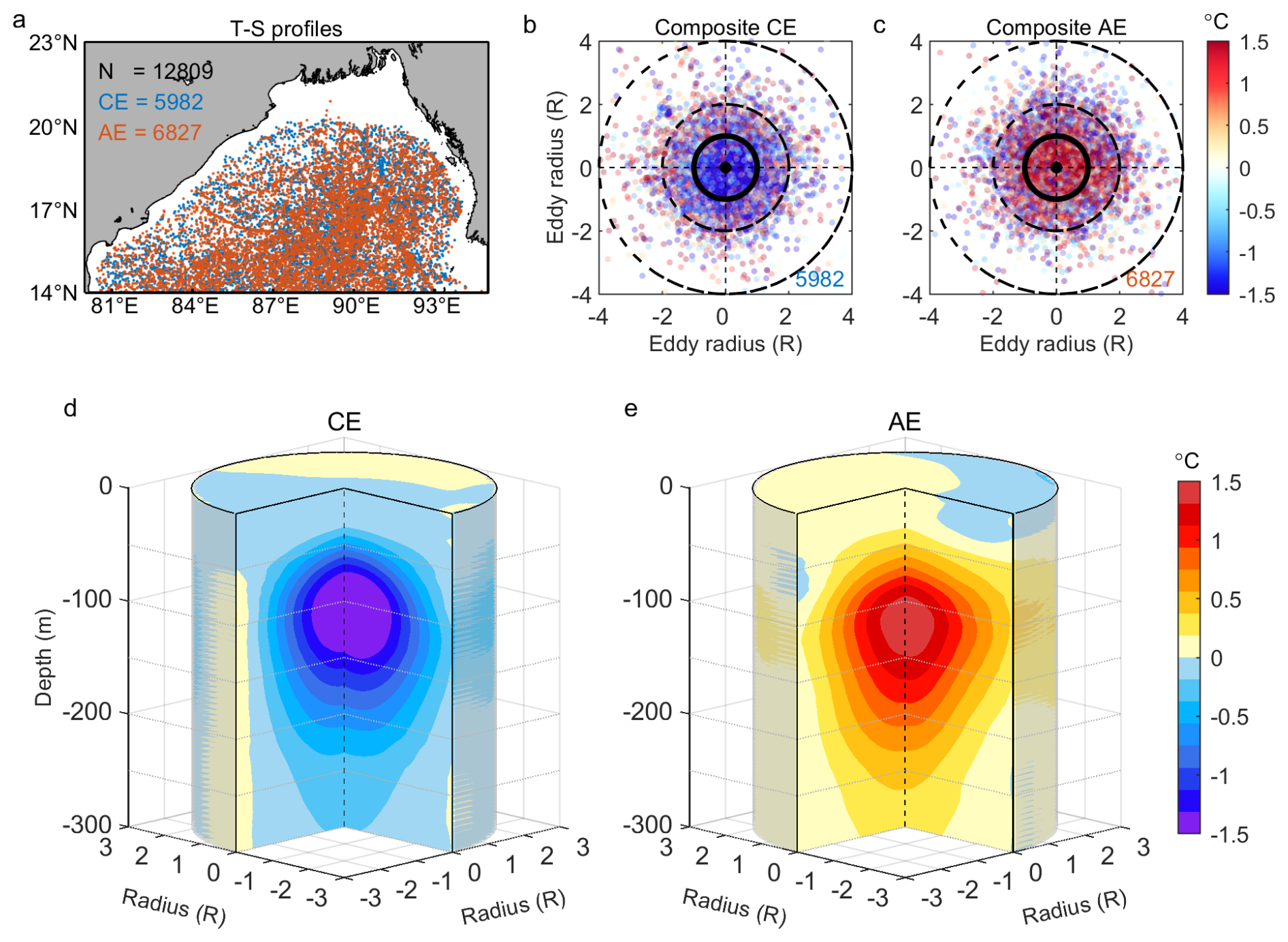
Figure 13 An example demonstrating the reconstruction of mean three-dimensional eddy temperature anomaly structures. (a) Geographic distribution of eddy-collocated temperature and salinity (T-S) profile data in the northern Bay of Bengal. The red and blue dots denote the profiles collocated with anticyclonic eddies (AE) and cyclonic eddies (CE), respectively. (b–c) Spatial distributions of the cyclonic and anticyclonic eddy-collocated profiles (in a) in radius-normalized eddy‐centric coordinates. The colors are the observed temperature anomalies relative to climatological monthly mean state at the depth of 100 m. (d–e) Reconstructed mean three-dimensional eddy temperature anomaly structures by interpolating the profile observations in (b)–(c) to standard 0.1R×0.1R grid boxes using ordinary kriging interpolation at each depth.

The ability to reconstruct regional three-dimensional eddy structures enables systematic interregional comparisons of eddy vertical structure that cannot be achieved using a simple inside/outside eddy classification. Using the collocated profile dataset, we derived mean west–east sections of eddy-induced temperature anomaly in several representative regions, including the South China Sea, the tropical southeastern Indian Ocean, the Kuroshio Extension, the Gulf Stream, the southeastern Pacific Ocean, the Southern Ocean, the Agulhas System, and the Brazil‐Malvinas Confluence (Fig. 14). The resulting composite structures successfully reproduced previously reported regional characteristics, including the relatively weak (∼ 1 °C) and shallow (∼ 100 m) eddy cores in the tropical southeastern Indian Ocean and the South China Sea (He et al., 2018; Sun et al., 2018; Yang et al., 2015), the deeper anticyclonic eddy cores relative to cyclonic eddies in the southeastern Pacific (Chaigneau et al., 2011), and the strong, deep penetrating (> 1000 m) eddy signals in midlatitude main current systems (Dong et al., 2017; Frenger et al., 2015; Laxenaire et al., 2019; Mason et al., 2017). Direct comparison of the reconstructed eddy structures across regions reveals substantial geographic variability in eddy vertical characteristics. Specifically, the intensity and vertical extend of temperature anomalies in the tropical southeastern Indian Ocean and the South China Sea are less than half of those in the midlatitude main currents. In addition, among the western boundary currents, the core depth and penetration depth of eddy-induced temperature anomalies in the Gulf Stream exceed those in the Kuroshio Extension and the Brazil–Malvinas Confluence by more than 300 m. These pronounced regional contrasts underscore the importance of background oceanographic conditions in shaping eddy structure and may help explain geographic differences in eddy-driven physical and biogeochemical processes.

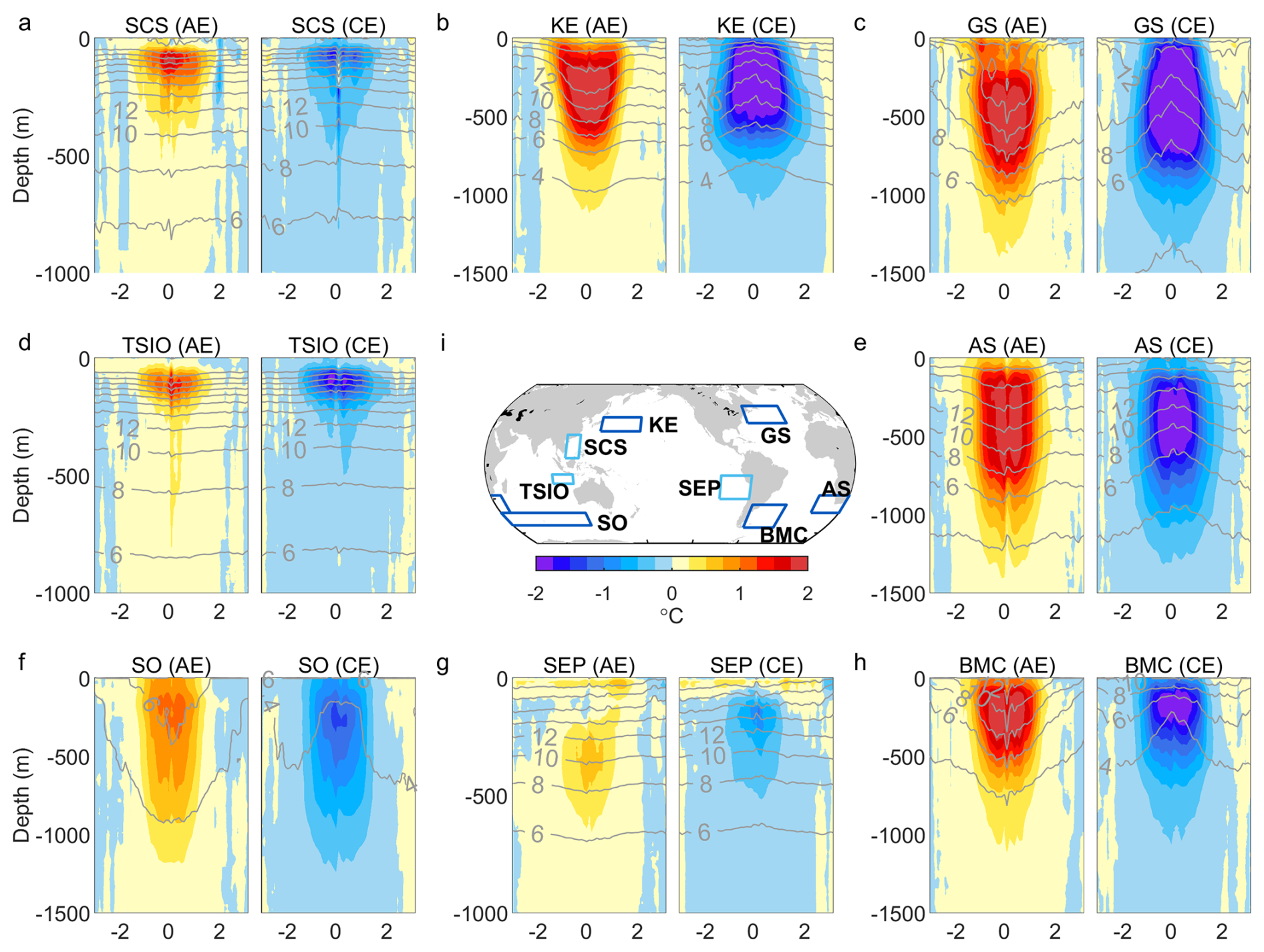
Figure 14 Composite mean eddy temperature anomaly structures in representative regions of the global ocean. (a–h) West-east sections of mean temperature anomalies across the composite centers of anticyclonic (AE) and cyclonic (CE) eddies in the South China Sea (SCS), the Kuroshio Extension (KE), the Gulf Stream (GS), the tropical southeastern Indian Ocean (TSIO), the Agulhas System (AS), the Southern Ocean (SO), the southeastern Pacific Ocean (SEP), and the Brazil‐Malvinas Confluence (BMC). (i) The statistical regions (boxes) of (a)–(h).

In addition to temperature, the dataset enables the concurrent reconstruction of three-dimensional eddy-induced salinity anomaly structures (Fig. 15). The results show that, although eddies in the tropical southeastern Indian Ocean and the South China Sea exhibit comparable temperature anomalies, salinity anomalies in the former are substantially stronger and penetrate deeper. Another notable feature is observed in the Kuroshio Extension, the Southern Ocean, and the Brazil–Malvinas Confluence regions, where salinity anomalies within anticyclonic eddies are positive above approximately 700 m but negative below this depth, with the opposite pattern observed within cyclonic eddies. This vertical sign reversal contrasts sharply with the temperature anomalies, which generally retain the same sign throughout the upper ocean (Fig. 14). Direct comparison with the background salinity structure (gray contours in Fig. 15) suggests that the sign reversal is likely associated with the vertical displacement of subsurface salinity minimum layer (McGillicuddy, 2016). An interesting phenomenon occurs in the Southern Ocean, where anticyclonic eddies are characterized by uplifted isohalines but depressed isotherms (Figs. 14e and 15e). This contrasting thermohaline response suggests that vertical displacement alone may not fully explain the observed anomalies and that eddy trapping of warm and saline subtropical water could play an important role. Because salinity is less directly affected by air–sea heat exchange and therefore behaves more conservatively than temperature (McDougall, 2003), combining salinity and temperature anomaly structures provides stronger observational constraints on the processes governing regional eddy-induced thermohaline variability.

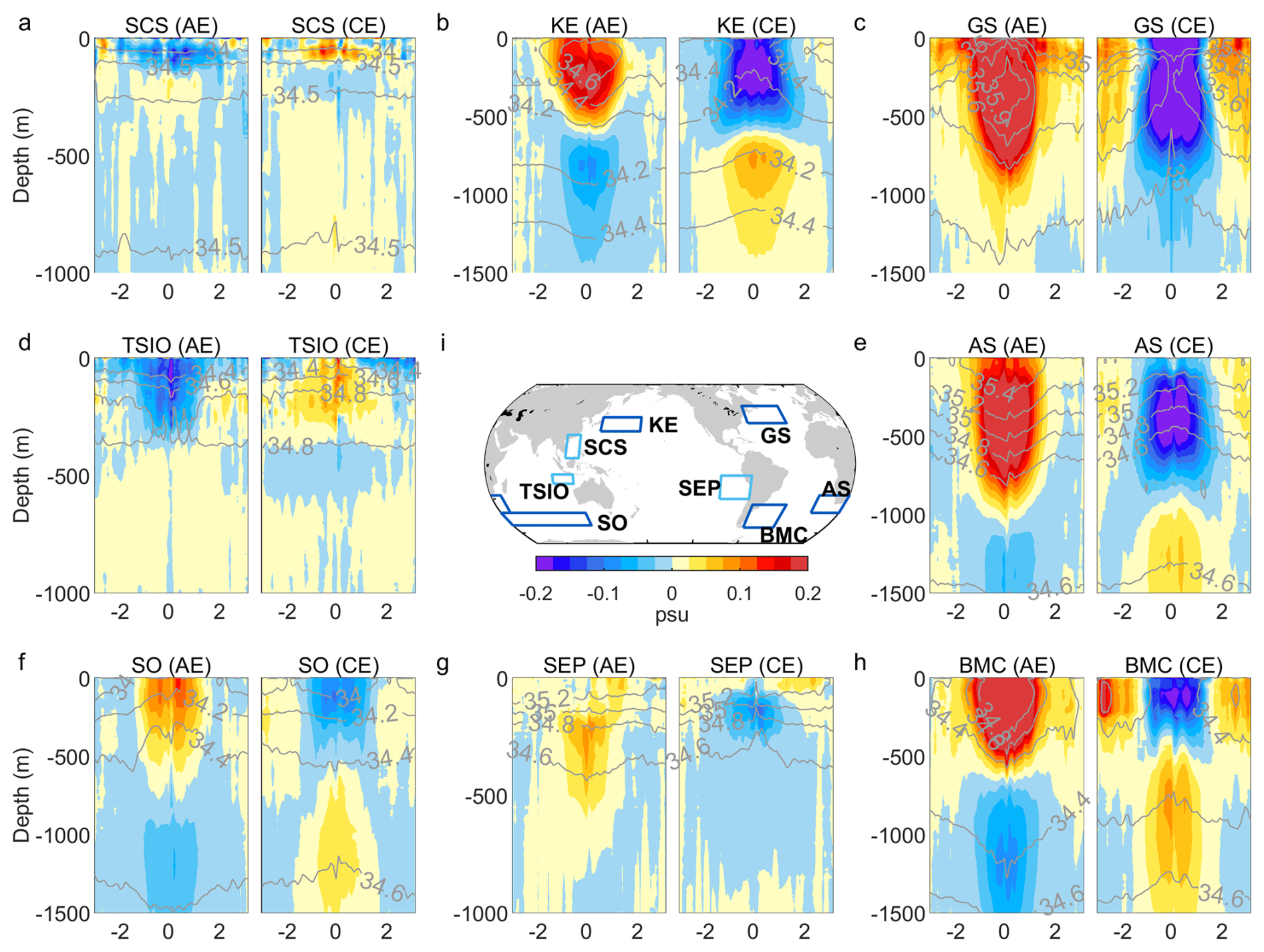
Figure 15 The same as Fig. 14, but for eddy salinity anomaly structures.

4.2 Global eddy thermohaline impacts

The extensive spatial coverage and large sample size of this dataset enable the characterization of eddy-induced temperature and salinity anomalies on relatively fine statistical grids (e.g., 2° × 2°), providing a global view of the spatial heterogeneity of eddy impacts (Figs. 6–7 and 11–12). Beyond serving as a validation of the dataset, these maps demonstrate its capability to resolve regional variability in eddy-induced thermohaline anomalies across the global ocean. For temperature, the strongest near-surface anomalies (with magnitudes exceeding 2 °C) occur in energetic regions such as western boundary currents and the Antarctic Circumpolar Current, where mesoscale eddy activity is most intense (Martínez-Moreno et al., 2021). At subsurface depths (e.g., 200 m), pronounced temperature anomalies are also evident within subtropical gyres, despite their comparatively weaker eddy kinetic energy (Figs. 6f and 7f). This pattern is consistent with previous studies showing that eddy-induced vertical displacement can generate large temperature anomalies in regions characterized by strong thermocline stratification (de Marez et al., 2019; Yang et al., 2013). Below this depth, temperature anomalies generally weaken with depth, although significant signals persist below 800 m in several major current systems, supporting earlier findings that mesoscale eddies can influence the deep ocean in dynamically active regions (Frenger et al., 2015; Sun et al., 2017). Notably, the penetration of temperature anomalies in the Gulf Stream is systematically deeper than in the Kuroshio Extension, despite comparable levels of eddy kinetic energy in the two regions (Martínez-Moreno et al., 2021). This result highlights that eddies with similar surface signatures can exhibit markedly different subsurface structures. The dataset therefore provides important observational constraints on the subsurface characteristics of mesoscale eddies that are not discernible from satellite observations alone.

Compared with temperature, eddy-induced salinity anomalies exhibit substantially greater spatial complexity (Figs. 11 and 12). Near the surface, anticyclonic eddies are associated with positive salinity anomalies in western boundary current regions but negative anomalies in tropical and subtropical regions, with the opposite pattern observed for cyclonic eddies (Figs. 11a and 12a). This large-scale contrast is consistent with previous studies that highlighted the influence of subsurface salinity maximum layers on the salinity response to eddy-induced vertical displacement (Yang et al., 2013). Below the subsurface salinity maximum layer (around 200 m), the same vertical displacement leads to depression of warm and salty water, thus resulting in positive temperature and salinity anomalies (Figs. 11f and 12f). At greater depths (e.g., 800 m), an interesting feature is the negative (positive) salinity anomalies within anticyclonic (cyclonic) eddies in the North Pacific and south of the ACC, opposing to the anomalies in the upper layer and at lower latitudes (Figs. 11k and 12k). This phenomenon is likely attributable to the depress (uplift) and/or poleward transport of subsurface salinity minima water at these depths (Mo et al., 2024).

Previous analyses based on earlier versions of the eddy-collocated profile archive have documented many of these regional characteristics (He et al., 2024a; Mo et al., 2024). The substantially expanded profile archive provided here more than doubles the available observational sampling, providing new opportunities to investigate eddy-induced thermohaline anomalies at finer spatial and temporal scales. Such improved sampling may facilitate future analyses of seasonal eddy structure variability and the evolution of eddy structure throughout the eddy life cycle, including the changes in core intensity, penetration depth, heat-content anomalies, and associated heat and salt transports (Laxenaire et al., 2019, 2020). More broadly, because eddies dynamics redistribute not only temperature and salinity but also nutrients, dissolved oxygen, pH, and other biogeochemical properties (Ellwood et al., 2020; Keppler et al., 2024; Xu et al., 2016), the dataset can also provide an important observational basis and physical constraint for studies of eddy impacts on marine biogeochemical environments.

4.3 Eddy effects on mixing and stratification

Because temperature and salinity determine seawater density, eddy-induced thermohaline anomalies can modify upper-ocean stratification and mixed-layer properties. As an illustrative application, we estimated the mean mixed-layer depth (MLD) anomalies within cyclonic and anticyclonic eddies, respectively, within each 2° × 2° grid box across the global ocean. MLD here was calculated for each profile as the depth at which the increase in potential density relative to the surface equals the increase in surface potential density associated with a 0.5 °C decrease in sea-surface temperature (de Boyer Montégut et al., 2004). At the global scale, anticyclonic eddies are generally associated with a shallower mixed layer, whereas cyclonic eddies are associated with a deeper mixed layer, with typical anomaly magnitudes of 10–20 m (Fig. 16). The strongest MLD anomalies occur in the Gulf Stream and the ACC regions, where anomaly magnitudes frequently exceed 50 m and locally approach 100 m. These large-scale patterns are consistent with previous observational analyses of eddy-induced mixed-layer variability (Gaube et al., 2019; Hausmann et al., 2017), providing further evidence that the dataset captures the major upper-ocean impacts of mesoscale eddies.

Figure 16 Geographic distribution of mean MLD anomalies within anticyclonic eddies (AE, left) and cyclonic eddies (CE, right). The right panel is the zonal mean of the left panels.

Compared with temperature and salinity anomalies, eddy-induced MLD anomalies exhibit less spatially coherent patterns, particularly at mid and high latitudes. This likely reflects the strong sensitivity of MLD estimates to small vertical variations in temperature and salinity (de Boyer Montégut et al., 2004), which can introduce substantial uncertainty when sampling is limited. Nevertheless, the expanded observational data enables the characterization of eddy-induced mixed-layer variability at a finer spatial resolution of 2° × 2°. Compared with the 5° × 5° climatology of Gaube et al. (2019), the resulting maps reveal finer-scale spatial heterogeneity, particularly in dynamically active regions such as the ACC and Gulf Stream (Fig. 16). This improvement highlights the potential of the expanded profile archive for resolving regional eddy impacts that may be obscured in coarser statistical products. More broadly, the successful mapping of MLD anomalies demonstrates the potential of this dataset for investigating other stratification-related properties, including thermocline depth, thermocline thickness, barrier-layer thickness, and upper-ocean stratification strength (Chen and Chen, 2020; Chen et al., 2021; de Boyer Montégut et al., 2007). Such applications may provide new insights into the role of mesoscale eddies in regulating upper-ocean mixing and water-mass exchange processes.

4.4 Eddy contribution to extreme temperature events

Given the ability of eddies to generate substantial temperature anomalies, they may contribute to extreme ocean temperature events, including marine heatwaves and cold-spells (Oliver et al., 2021; Schlegel et al., 2021). Because the present dataset is based on discrete profile observations rather than continuous time series, we focus on extreme temperature anomalies, which can serve as useful proxies for extreme temperature events (He et al., 2024b). Using this dataset, we quantified the contribution of mesoscale eddies to temperature extremes by calculating the percentage of extreme temperature anomalies occurring within eddy interiors within each 2° × 2° grid box (Fig. 17). Extreme high (low) temperature anomalies here were identified as temperature anomalies exceeding the 95th (falling below the 5th) percentile of all temperature anomalies within each grid box during the study period between 1993 and 2021. Given that anticyclonic (cyclonic) eddies are generally associated positive (negative) temperature anomalies, they are expected to contribute preferentially to extreme high (low) temperature anomalies. Therefore, we focus on the fraction of extreme high temperature anomalies occurring within anticyclonic eddies and extreme low temperature anomalies occurring within cyclonic eddies.

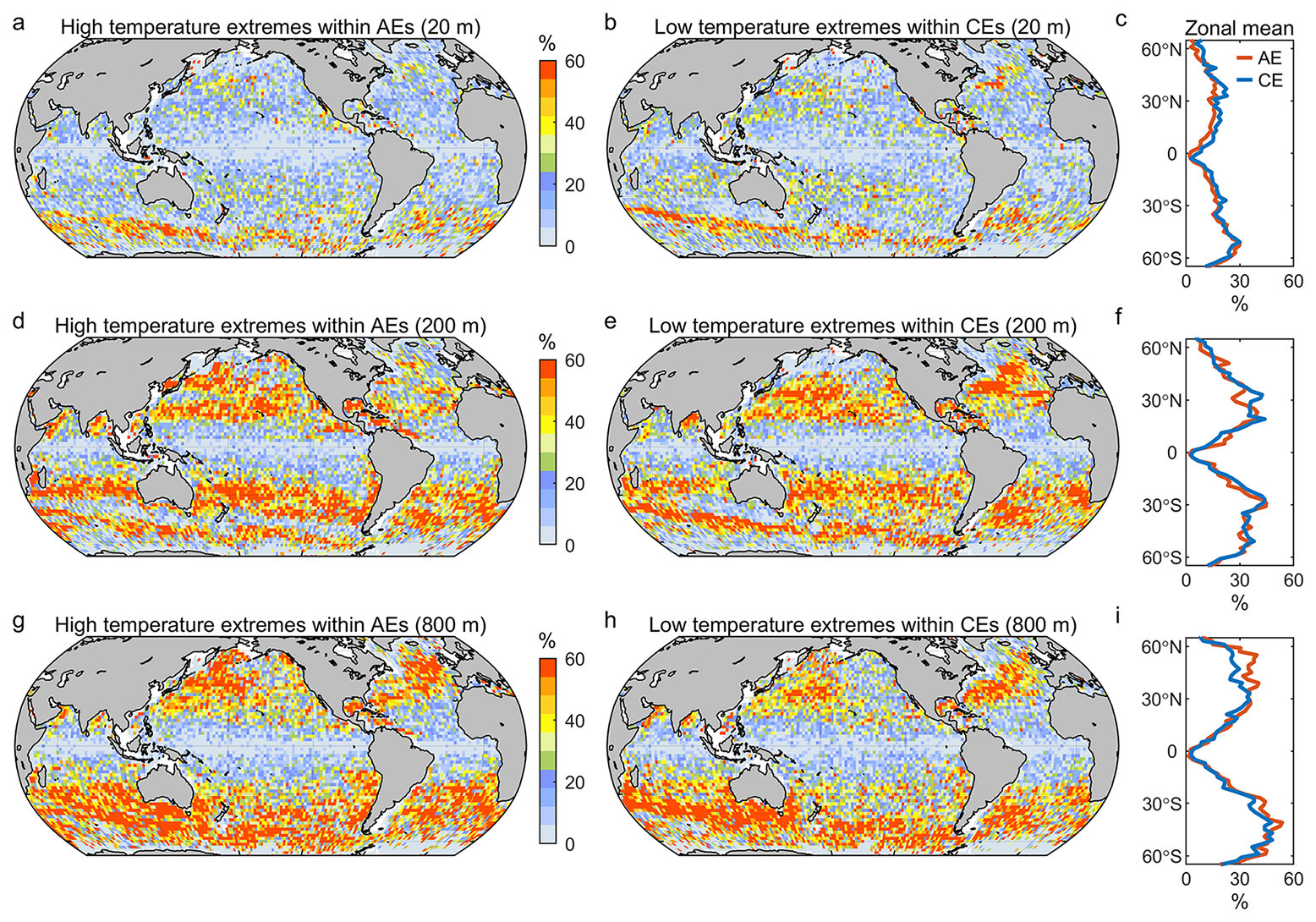
Figure 17 Spatial variability in eddy contribution to extreme temperature events in the upper ocean. (a–h) Global distribution of the percentages of extreme high temperature anomalies occurred within anticyclonic eddies (AE, left), extreme low temperature anomalies occurred cyclonic eddies (CE, middle), and the corresponding zonal averages (right) at the depths of 20, 200, and 800 m, respectively.

At the global scale, this fraction is typically around 10 % near the surface, except in the ACC region values can reach up to 30 % (Fig. 17a–c). These percentages are close to the overall probability of eddy occurrence (Fig. 5), suggesting that mesoscale eddies do not noticeably enhance the occurrence of surface temperature extremes. In contrast, the contribution of mesoscale eddies increases markedly below the surface. At 200 m depth, approximately half of extreme high (low) temperature anomalies in subtropical gyres and western boundary current regions occur within anticyclonic (cyclonic) eddies (Fig. 17d–f). Similar patterns remain evident at depths of up to 800 m (Fig. 17g–i), highlighting the important role of mesoscale eddies in shaping subsurface temperature extremes. These results are generally consistent with those reported by He et al. (2024b), providing further evidence that the dataset captures the major characteristics of eddy contributions to extreme temperature anomalies. Compared with the previous analysis based on 5° × 5° grid boxes, the expanded profile archive enables these relationships to be characterized at a substantially finer spatial resolution (2° × 2°), revealing greater regional variability in eddy–extreme temperature relationships. The dataset therefore provides an improved observational basis for future investigations of mesoscale eddy influences on marine heatwaves, cold spells, extreme salinity anomalies, and other ocean extremes.

4.5 Eddy-driven heat and salt transports

The dataset enables the characterization of the vertical structure of eddy-induced temperature and salinity anomalies across the global ocean. Combined with satellite-derived information on eddy occurrence probability, rotational velocity, and movement speed, these observations provide an observational basis for estimating eddy-induced heat and salt transports and for identifying regions where mesoscale eddies may contribute substantially to tracer redistribution. Furthermore, by interpolating the eddy-collocated profiles to a standardized three-dimensional coordinate system, the dataset can be used to reconstruct the composite three-dimensional thermohaline structure of mesoscale eddies (Fig. 13), and subsequently horizontal geostrophic velocity and potential vorticity fields (Chen et al., 2012; Yang et al., 2015). These products could subsequently support estimates of heat, salt, and water-mass transports associated with eddy stirring and rotational motions (Sun et al., 2019). At present, the available profile density may still be insufficient to robustly reconstruct mean three-dimensional eddy structures in relatively small regions (e.g., 2° × 2° grid boxes). Nevertheless, the continuing growth of the global in situ observing system will provide opportunities to improve the spatial resolution and robustness of regional eddy reconstructions. Such developments may facilitate more detailed assessments of the role of mesoscale eddies in water-mass transport, heat and salt redistribution, and ocean heat balance from regional to global scales.

4.6 Eddy response to climate change

Understanding how mesoscale eddies respond to and interact with long-term ocean warming remains an important challenge in climate research. Because eddy-induced thermohaline anomalies directly reflect the influence of mesoscale eddies on ocean temperature and salinity distributions, their long-term variability provides a useful observational indicator of changing eddy impacts under a warming climate. Progress in this area has been limited by the lack of long-term, observation-based records of eddy thermohaline structure. The present dataset provides 5.46 million eddy-collocated temperature and salinity profiles spanning the period 1993–2021. Although profile numbers remain relatively limited before 2003 (< 100 000 profiles yr⁻¹), the dataset contains more than 200 000 profiles annually thereafter (Fig. 4c). This extensive observational archive provides opportunities to investigate temporal changes in eddy-induced thermohaline anomalies in densely sampled regions, such as the northwestern Pacific, and north Atlantic, and north Indian Ocean (Fig. 4a). Such analyses may help improve understanding of how mesoscale eddy impacts have evolved in response to ongoing ocean warming (Fig. 10). More broadly, the dataset provides a long-term observational benchmark for evaluating the ability of ocean and climate models to simulate eddy-induced thermohaline variability and its role in ocean heat uptake, heat redistribution, and climate variability change (Jing et al., 2020; Rackow et al., 2022; Wang et al., 2024; Westen and Dijkstra, 2021).

5 Limitations of the collocated dataset

Although this dataset provides a comprehensive observational resource for investigating eddy-induced thermohaline anomalies and transports from regional to global scales, several limitations should be considered when using the product. First, mesoscale eddies were identified from satellite altimetry and therefore only eddies with sufficiently strong sea surface height anomaly signatures can be detected. Consequently, eddies during their formation and dissipation stages may be underrepresented. In addition, although the META eddy product used in this study is among the most widely used global eddy datasets, it has known limitations in representing eddy splitting and merging processes, which may introduce uncertainties in profile–eddy associations during such events (Ioannou et al., 2024; Laxenaire et al., 2018). Second, satellite observations characterize only the surface expression of mesoscale eddies. Beneath the surface, eddies may exhibit vertically tilted structures, subsurface-intensified cores, or other forms of structural variability (Laxenaire et al., 2019; Zhang et al., 2016, 2017). Through composite averaging, the present dataset can reconstruct the mean three-dimensional eddy structure within a target region and reveal systematic regional differences among eddies. However, individual eddies may deviate substantially from the regional mean structure, and such composite analyses may not capture the full range of individual eddy variability. Third, during the collocation procedure, each profile was assigned to its nearest eddy to avoid multiple associations. Although this approach provides a consistent framework for large-scale statistical analyses, hydrographic conditions may occasionally be influenced by multiple neighboring eddies, particularly in regions of dense eddy activity or strong eddy–eddy interactions. Such effects are expected to occur primarily near eddy boundaries and are therefore likely to have a limited influence on estimates of eddy-core thermohaline anomalies. Finally, subsurface and deep-ocean eddies that do not produce detectable sea surface height anomaly signatures cannot be represented in the present dataset. Consequently, the thermohaline structures, transports, and environmental impacts associated with these eddies remain unresolved and require dedicated observational approaches beyond satellite-altimetry-based eddy identification.

6 Data availability

The eddy-collocated T-S profile data product used in this manuscript is publicly available at https://doi.org/10.5281/zenodo.20607854 (He, 2026) and https://data.scsio.ac.cn/metaData-detail/2076524929418170368 (last access: 9 June 2026). The quality-controlled and bias-corrected WOD temperature and salinity profile dataset (CODC-v2) is available at http://www.ocean.iap.ac.cn/ftp/cheng/CODCv2_Insitu_T_S_database/ (last access: 20 April 2026). The original WOD temperature and salinity profile dataset is available at https://www.nodc.noaa.gov/OC5/WOD/pr_wod.html (last access: 7 May 2025). The eddy product is delivered by the AVISO⁺ at https://www.aviso.altimetry.fr/en/data/products/value-added-products/global-mesoscale-eddy-trajectory-product/meta3-2-dt.html (last access: 27 September 2022). The climatology sea water temperature data (WOA 2023) is available at https://www.ncei.noaa.gov/access/world-ocean-atlas-2023/ (last access: 9 December 2025).

7 Conclusions

We developed a global eddy-collocated temperature and salinity profile dataset by integrating 29 years (1993–2021) of in situ hydrographic observations with satellite-derived mesoscale eddy information. The dataset provides 5.46 million temperature–salinity profiles associated with individual mesoscale eddies and includes both hydrographic properties and their corresponding anomaly fields relative to climatology. By linking subsurface observations with eddy characteristics, the dataset provides a global observational framework for investigating the three-dimensional thermohaline signatures of mesoscale eddies. The dataset successfully reproduces many previously reported characteristics of eddy-induced temperature and salinity anomalies across diverse oceanic regimes, including their vertical structures, regional variability, and impacts on upper-ocean stratification. The substantially expanded observational sampling also enables analyses at finer spatial scales than previously possible, revealing pronounced regional heterogeneity in eddy-induced thermohaline anomalies, mixed-layer perturbations, and extreme temperature variability throughout the upper 1000 m of the ocean. These results demonstrate that the dataset provides a robust observational basis for characterizing the regional variability of eddy impacts on oceanic thermohaline structure across the global ocean. Beyond these applications, the dataset provides new opportunities to investigate a broad range of eddy-related processes, including heat and salt redistribution, water-mass transport, ocean temperature extremes, long-term changes in eddy thermohaline properties, and eddy biogeochemical impacts. As the global observing system continues to expand, future updates of the dataset may further improve observational coverage and statistical robustness, particularly at regional scales. More broadly, this dataset provides a long-term, observation-based benchmark for evaluating ocean and climate model simulations and contributes to a better understanding of the role of mesoscale eddies in regulating ocean circulation, heat uptake, and climate variability.