A decade of monthly frontal ablation at 147 tidewater glaciers in Svalbard

We present a regional-scale monthly analysis of frontal ablation at 147 tidewater glacier basins in Svalbard from January 2015 through December 2024. A multi-temporal, deep-learning segmentation model was implemented to reduce the manual labor cost of mapping 203 294 terminus positions, yielding 15 647 monthly-averaged calving fronts derived from Sentinel-1 SAR imagery. In addition, a monthly ice discharge time series is developed from the ITS_LIVE velocity database, as well as regionally existing ice thickness products. To account for ice mass loss due to surface processes between the fluxgate and terminus (i.e. the glacier domain), the climatic mass balance is integrated over the domain area using monthly aggregated daily outputs from the MAR regional climate model. The result is a high spatio-temporal resolution frontal ablation time series (15 500 monthly estimates), allowing new insights and progress towards a process understanding of frontal ablation. The mean annual frontal ablation rate across all glaciers from 2015 to 2024 is 21.57±0.97 Gt yr⁻¹. The Austfonna ice cap accounts for ∼48 % of Svalbard's frontal ablation, due to the dominant Austfonna Basin 3, with a 5.05±0.35 Gt yr⁻¹ annually averaged rate. As frontal ablation measurements have historically been limited to annual and decadal temporal resolution, this dataset addresses the intra-annual and seasonal variability knowledge gap, while providing valuable reference data for the modeling community. The frontal ablation, ice discharge, and calving front time series are publicly available at https://doi.org/10.5281/zenodo.19481461 (Pyles et al., 2026).

1 Introduction

Glaciers terminating in bodies of water lose mass through frontal ablation at the ice-water and ice-air interfaces. Defined as mass lost along the near-vertical calving front, frontal ablation collectively describes several mass loss processes including subaqueous melting, subaerial sublimation and melting, and iceberg calving (Cogley et al., 2011). As frontal ablation is a fundamental contributor to tidewater glacier mass balance (Huss and Hock, 2015), accurate quantification and partitioning of the mass loss components is crucial for assessing its controls (Kochtitzky et al., 2022a, b) and calibrating models (Malles et al., 2023; Recinos et al., 2022; Rounce et al., 2023; Zekollari et al., 2024). Individual frontal ablation processes significantly contribute to mass budgets, as calving accounts for an estimated 32 % of marine-terminating glacier mass loss in Svalbard and ∼16 %–25 % of Svalbard's total ice loss (Błaszczyk et al., 2009; Hagen et al., 2003). Similarly, several case studies indicate that subaqueous melting is an important control on the mass loss and dynamics of tidewater glaciers, with melt rates up to ∼3–9 m d⁻¹ (Bartholomaus et al., 2013; Fried et al., 2015; Sutherland et al., 2019). Because calving and submarine melting are physically complex processes, likely influencing each other (Ma and Bassis, 2019; Slater et al., 2018; Wagner et al., 2019), frontal ablation has been difficult to constrain and remains a major uncertainty in current cryosphere research (Schuler et al., 2020). Resolving frontal ablation's contribution to glacier and regional mass budgets at high temporal resolutions (i.e. annual and seasonal) is important for understanding the spatial heterogeneity and temporal variability of frontal ablation (Kochtitzky et al., 2022a; Schuler et al., 2020).

Though recent studies have computed frontal ablation of tidewater glaciers on regional extents (Kochtitzky et al., 2022b; Temme et al., 2025), the estimates are often calculated on multi-annual or decadal timescales, leaving a knowledge gap in the temporal evolution, and consequently, the process understanding of frontal ablation. The coarse temporal resolution is largely due to the demanding nature of frontal ablation computation. Ice discharge (velocity and thickness), climatic mass balance (CMB), and frontal area change datasets are required to fully resolve and partition the frontal ablation components. However, much of the data is difficult to obtain and aggregate on consistent spatio-temporal scales. Of the most time- and labor-intensive tasks, Kochtitzky et al. (2022b), McNabb et al. (2015), and Minowa et al. (2021) manually mapped ∼4500, >10 000, and 3969 calving front positions, respectively, to estimate mass change at the terminus.

In contrast, several studies have achieved annual or seasonal frontal ablation estimates, each with different methodological or spatial limitations. While Osmanoğlu et al. (2013, 2014) provided annual frontal ablation analysis for King George Island and Livingston Island in the South Shetland Islands archipelago, they did not account for mass changes due to variations in the calving fronts. Currently, McNabb et al. (2015), Minowa et al. (2021), and Fahrner et al. (2025) are the only regional scale studies that partitioned ice discharge and terminus mass changes at annual or seasonal resolution. However, each study calculated frontal ablation for a select subset of tidewater glaciers across their broader study regions; McNabb et al. (2015) considered 27 Alaskan glaciers with large, active calving fronts and aggregated frontal ablation annually over 1985–2013, Minowa et al. (2021) derived annual estimates for 38 major glaciers in the Patagonia icefields between 2000–2019, and Fahrner et al. (2025) delivered a seasonal (3-monthly) frontal ablation dataset for 49 tidewater glaciers on the Greenland Ice Sheet from 1987–2020.

With the increasing availability of Earth Observation and globally modeled datasets (Farinotti et al., 2019; Gardner et al., 2025; Hugonnet et al., 2021; Millan et al., 2022), as well as the development of deep-learning based segmentation algorithms (Gourmelon et al., 2022a; Herrmann et al., 2023; Mohajerani et al., 2019; Zhang et al., 2021), the previously high data and labor demands may be bypassed, enabling frontal ablation estimation at high temporal resolution on a full-regional scale. To address the community's demand for annually and seasonally resolved frontal ablation estimates, we developed an approach that leverages the recent data and technological advancements, chiefly, by implementing a multi-temporal calving front segmentation model to automate terminus delineation (Dreier et al., 2026a, b). Similarly, Li et al. (2024) generated just under 125 000 calving front positions across 149 tidewater glaciers in Svalbard from 1985–2023 using an automated deep-learning framework. In a subsequent study, Li et al. (2025) discovered pervasive glacier retreat across Svalbard, with apparent seasonality in calving front positions for 86 of 138 non-surging glaciers, however, the scope was limited to oceanic and atmospheric controls on terminus position. To extend the automated workflow analysis, we apply a novel routine to generate a monthly frontal ablation dataset across Svalbard's marine-terminating glaciers between 2015–2024, marking the first frontal ablation study produced from model-derived terminus segmentations.

2 Study region

Situated between 76 and 81° N, Svalbard is an Arctic region surrounded by the Greenland and Barents Seas in the south and the Arctic Ocean to the north (Fig. 1). The geography of the Svalbard Archipelago is characterized by five main islands – Spitsbergen, Nordaustlandet, Edgeøya, Barentsøya, and Kvitøya – of which we subset into seven established glaciated regions (Li et al., 2025; Moholdt et al., 2010; Sochor et al., 2021; Wang et al., 2022): Northwest Spitsbergen (NW), Northeast Spitsbergen (NE), South Spitsbergen (SS), Barentsøya and Edgeøya (BE), Austfonna ice cap (AF), Vestfonna ice cap (VF), and Kvitøya (KV), an island (657 km²) predominately covered by the Kvitøyjøkulen ice cap. Kvitøyjøkulen is a key contributor to Svalbard's frontal ablation (Kochtitzky et al., 2022a), as the 100 km calving front ice cliffs constitute ∼90 % of the island's coastline (updated from Bamber and Dowdeswell, 1990).

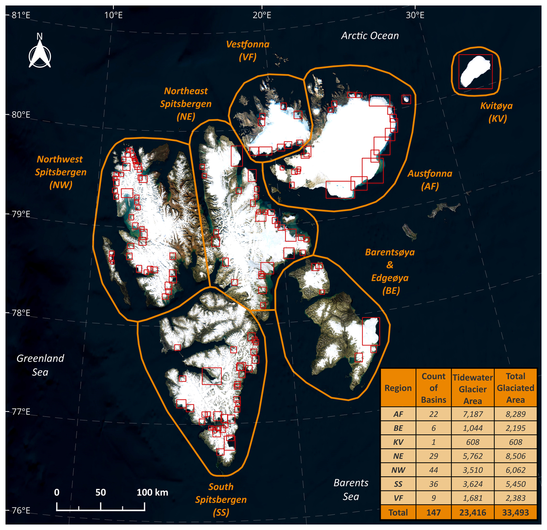
Figure 1 Geographic map of Svalbard, split into seven distinct regions. Spitsbergen (NW, NE, SS) is characterized by rugged topography, compared to the low-elevation ice caps of the Edgeøya (south BE), Kvitøya (KV), and Nordauslandet (AF, VF) islands. The subregions are distinguished by Randolph Glacier Inventory version 6 (RGI Consortium, 2017) basins (red boxes) corresponding to marine-terminating glaciers, as well as the tidewater glacier drainage area (km²) and total glacierized area (km²) in the provided table. Overall, 151 tidewater glaciers compose 147 defined basins, where a monthly frontal ablation time series is produced from January 2015 through December 2024. Background imagery provided from the Bing Satellite ©.

Svalbard's tidewater glaciers and outlet areas vary in size, shape, flow style, and geographic setting. From the 151 tidewater glaciers distinguished in this study, 53 have a terminus length less than 2 km, 56 are between 2–5 km, and 42 are greater than 5 km. In total, ∼900 km of terminus length was exposed to frontal ablation in 2024, an increase from ∼835 km in 2015. The AF, BE, and KV subregions are distinguished by large ice cap style glaciers whose termini splay outward to the ocean, while the VF, NW, NE, and SS regions have more traditional fjord-style glaciers with constrained flow. Several glaciers are protected by natural land inlets or isles, while most have an unobstructed ocean interface. In addition, marine-terminating glaciers in Svalbard have historically exhibited surge-type behavior, particularly on the largest island, Spitsbergen (Błaszczyk et al., 2009; Dowdeswell et al., 1991; Farnsworth et al., 2016; Jiskoot et al., 1998; Szafraniec, 2020). Given the diverse glacier geometries, outlet areas, flow types, and observed behavior of Svalbard's marine-terminating glaciers, the region is an ideal test site for this frontal ablation pilot study.

3 Methods

Frontal ablation is difficult to quantify directly, due to uncertainties in measuring or modeling subaqueous melt and the volume of calving events (Kochtitzky et al., 2022b; Truffer and Motyka, 2016). Therefore, to approximate the frontal ablation we use a fluxgate input-output method, where the fluxgate bounds an area of downstream ice between the gate and terminus. We refer to this bounded area as the glacier domain and calculate the mass budget within the domain, using the frontal ablation equation described in Minowa et al. (2021):

$$\begin{array}{}\text{(1)}& A_{\mathrm{f}}=S_{\mathrm{g}}{\displaystyle \frac{W_{\mathrm{f}}}{W_{\mathrm{g}}}}\dot{L}-D-{\dot{B}}_{\mathrm{f}}\end{array}$$

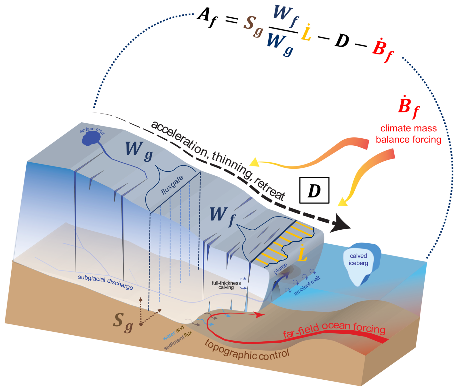
Figure 2 Frontal ablation schematic adapted from Catania et al. (2020) and annotated with Eq. (1) terms to visualize the relevant mass budget processes at a marine-terminating glacier. Ice discharge (D) is computed at the fluxgate, the CMB (${\dot{B}}_{\mathrm{f}}$) is estimated over the glacier domain between W_g and W_f, while the width-averaged frontal displacement rate ($\dot{L}$) is averaged between two timesteps of the terminus position (straight and sinuous blue lines) and S_g is the cross-sectional area at the fluxgate. Frontal ablation is primarily accounted for by calving events and ambient undercutting melt from the ocean, as well as subglacial discharge and localized meltwater plumes. By the equation's convention in Minowa et al. (2021), positive frontal ablation indicates terminus advance and/or ice thickening within the domain, opposed to frontal retreat and/or thinning for negative values.

where A_f is the frontal ablation, D is the ice discharge, ${\dot{B}}_{\mathrm{f}}$ is the climatic mass balance, S_g is the glacier's cross-sectional area at the fluxgate, $\dot{L}$ is the width-averaged frontal displacement rate, and W_f and W_g are the widths of the ice front and fluxgate, respectively (Fig. 2). The datasets and processing methods used to obtain a per-glacier monthly time series from January 2015 through December 2024 (hereafter commonly referred to as 2015–2024) for the components composing the equation – frontal area change, ice discharge, climatic mass balance – are described in subsections below.

3.1 Frontal area change

3.1.1 Sentinel-1 SAR imagery

Producing a monthly frontal area change time series requires consistent, year-round monitoring of the tidewater glaciers. The radar capabilities of the Sentinel-1 platform are well suited for this application, as the Sentinel-1A and 1B satellites provide regular imagery independent of weather conditions and solar illumination at the high latitudes of Svalbard. We use a Sentinel-1 Synthetic Aperture Radar (SAR) normalized radar backscatter product developed by the German Aerospace Center (DLR) and the Leibniz Supercomputing Center (LRZ) High-Performance Data Analytics platform, terrabyte (Truckenbrodt et al., 2023). The product is derived from Sentinel-1 Ground Range Detected data, radiometrically calibrated to gamma-naught (γ⁰), and provided as intensity imagery representing incidence angle normalized radar measurements. Additionally, to facilitate seamless user analysis, the product is terrain-corrected, denoised, projected, and geolocated (Albinet et al., 2022). We preprocess Sentinel-1 SAR imagery acquired in Interferometric Wide Swath mode (IW), for all but one glacier – the Kvitøyjøkulen ice cap (KV) in northeast Svalbard – to leverage the mode's high 10 m spatial resolution. For Kvitøyjøkulen, we use SAR images from the Extra Wide Swath (EW) acquisition mode with 40 m resolution, as IW mode data are unavailable. Scenes from all polarization channels – the co-polarized HH/VV and cross-polarized HV/VH – are included in the training dataset and the preprocessed imagery used to generate predictions with the segmentation model, which only takes one polarization at a time.

3.1.2 Multi-temporal segmentation model

To automate calving front delineation, we employed the deep-learning multi-temporal segmentation model Tyrion-T-GRU (Dreier et al., 2026b), which performs pixel-wise semantic classification of SAR imagery. From the predicted ice and ocean classes, the calving front can be extracted. In contrast to earlier architectures such as Tyrion and Hookformer (Gourmelon et al., 2025; Wu et al., 2024), which process individual images independently, Tyrion-T-GRU operates on time series of SAR imagery, allowing the model to observe a wider temporal context. The approach was further refined by adapting the input time series to include a static land mask of the study area and by ensuring that each sequence contained relatively unambiguous (“easy”) reference samples during model application (Dreier et al., 2026a), which helped stabilize the predictions. Additional details on the model architecture can be found in Gourmelon et al. (2025) and Dreier et al. (2026a).

3.1.3 RGI boxes and regional zone labels

A critical step for processing frontal area changes is defining a consistent sampling geometry for each Randolph Glacier Inventory version 6 (RGI) basin that contains at least one marine-terminating glacier. To identify all tidewater glaciers in Svalbard, we use the manually digitized termini polygons from summer 2019 in Kochtitzky et al. (2022b), hereafter called the “2019 polygons”; detailed mapping dates can be found at https://doi.org/10.5281/zenodo.19481461 (Pyles et al., 2026). We refer to the sampling geometries as “RGI boxes”, which are created by buffering the minimum bounding envelope of all 2019 polygons per RGI-ID by two kilometers, ensuring that the sampling extent captures all frontal changes (i.e. sustained retreat or advance) between 2015–2024. While rare, the position of an RGI box may be manually adjusted to facilitate an optimal sampling extent. In total, 147 RGI boxes are defined, encompassing 151 marine-terminating glaciers (defined by Kochtitzky et al., 2022b), with four RGI boxes containing two separate glaciers. The two distinct 2019 polygons in these four boxes (RGI60-07.00703, RGI60-07.00854, RGI60-07.01354, and RGI60-07.01482) have the same RGI v6 ID, and therefore in downstream tasks are processed together and handled as one RGI basin. Some RGI boxes have large spatial overlaps with adjacent boxes (i.e. glaciers that merge into a single terminus; RGI60-07.00296 and RGI60-07.00422), however, we retain such cases as individual glacier basins, consistent with their definition in Kochtitzky et al. (2022b). In addition to the RGI box vector geometry, a reference raster and geotransform are generated by rasterizing each box onto a 10 m spatial grid in the WGS84 UTM zone 33N coordinate reference system (EPSG:32633), enabling a consistent georeference for downstream raster processing.

To develop zone type labels for training the model to map Svalbard's calving fronts, we created a regional label for ice, ocean, and land, encompassing Svalbard and its marine-terminating glaciers (Fig. 3a). The process begins with building an updated glacier inventory by adjusting the RGI basin at the ice-ocean interface for all 151 glacier termini (Fig. 3c). Specifically, the existing RGI v6 calving front geometry is replaced with the 2019 polygon geometry from Kochtitzky et al. (2022b). Before updating the termini, initial regional-scale zone labels are produced using the Svalbard coastline extracted from OpenStreetMap (OpenStreetMap Contributors, 2024); all non-ice area (from RGI v6) inland of the coastline is defined as land, while all area within a 10 km buffer of the coastline's convex hull is defined as ocean. To produce accurate zone labels, we manually create intermediate glacier-specific ocean and land polygons centered around the terminus, which are designed to assist in merging the existing RGI and 2019 polygon together. For a visual reference, the intermediate ocean and land polygons are generated using the same optical image (Landsat-8) as the 2019 polygon was digitized from; the land polygon's function is to reclassify RGI area forward and lateral of the 2019 polygon as land, while the ocean polygon traces the ocean-ice and ocean-land interfaces with close precision, filling in retreated area with ocean if the 2019 polygon has retreated relative to the RGI terminus position (Fig. 3c). After applying the intermediate land and ocean layers, the updated terminus geometry is joined onto the largest upstream RGI basin boundary to inherit metadata attributes; because of the largest boundary merge criteria, some glaciers composed of multiple RGI basin ice trunks may receive metadata (RGI-ID and name) different from their established names in existing literature. Nevertheless, the resultant zone labels are highly detailed at each glacier's outlet area and serve as the ground truth for the segmentation model's training data (Fig. 3b).

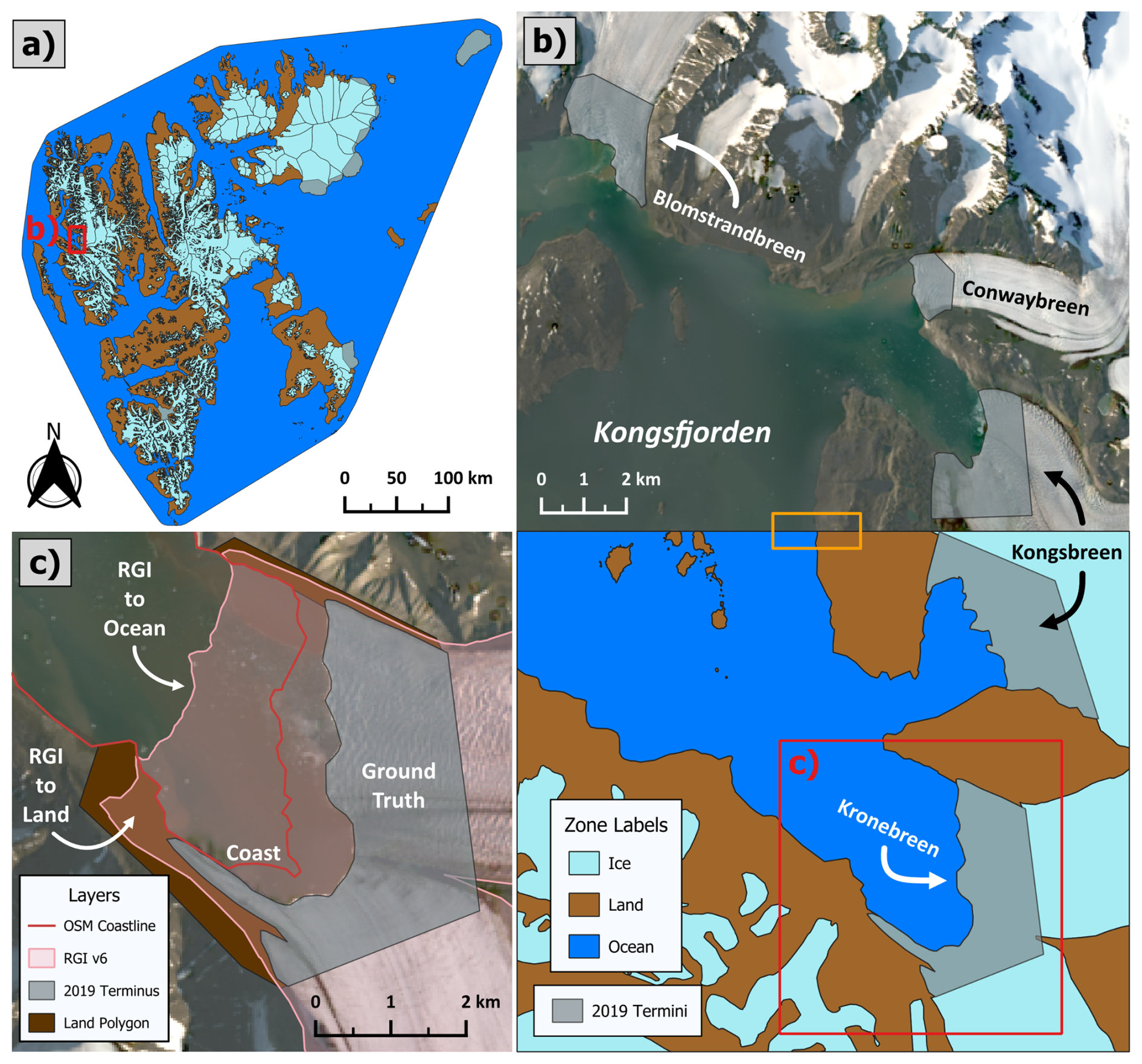
Figure 3 (a) Full Svalbard regional extent of the updated ice, ocean, and land zone labels. A red inset map of the zoomed window in (b) focuses on the Kongsfjorden where Kronebreen (c) is located. (b) Spatially contiguous top and bottom subpanels (see land-ocean area within orange box) of the Kongsfjorden and its four tidewater glaciers, showing zone label accuracy with respect to the reference optical image. The top panel shows the termini polygons manually delineated by Kochtitzky et al. (2022b) in 2019, with the Landsat-8 image (28 July 2019) they used for front mapping plotted as background. Bottom panel is the resulting zone labels at the terminus after applying the layers and processing steps in (c); compare Kronebreen in panels (c) and (b) for a before/after example. c) An overview for updating the RGI v6 ice extent at the Kronebreen terminus to the ground truth front position mapped by Kochtitzky et al. (2022b), which results in updated ocean and land zone labels around the glacier outlet area. The OpenStreetMap coastline (© OpenStreetMap contributors, https://www.openstreetmap.org/copyright, last access: April 2026) provides a reference for maintaining the land-ocean interface during zone label updates and assists in illustrating the enclosed RGI v6 areas (pink) that become land/ocean. The workflow is applied to all 147 tidewater glacier basins.

3.1.4 Training data generation and SAR image preprocessing

The segmentation model is pre-trained on the CaFFe benchmark dataset, comprised of 681 multi-mission (radar and optical) images across five glaciers in the Antarctic Peninsula, as well as one each in Alaska and Greenland (Gourmelon et al., 2022a). To improve the performance of the segmentation model at Svalbard, training data are developed for fine-tuning the model on the unseen Svalbard domain. The training data are built using SAR imagery over a two-month period from July-August 2019, coincident with the interval during which the 2019 polygons were manually digitized from optical images (Kochtitzky et al., 2022b). We create two styles of training data: (1) a glacier-style dataset, defined by the RGI box extent, and (2) a regional-style dataset, where full Sentinel-1 scenes are clipped to the Svalbard zone label extent defined by the ocean label bounds (Fig. 3a, blue area). The glacier-style dataset focuses on the glacier outlet area, allowing the model to learn a glacier's environment where the detailed zone labels were manually curated (Fig. 4a). Two glaciers – Austre Torellbreen and Vestre Torellbreen in southwest Svalbard – lack training data, as their reference polygons were digitized in August 2017 due to inadequate optical imagery over the 2019 period; despite exclusion from the training set, we still predict the terminus position from the available SAR time series. The regional-style dataset gives the model a broader scope of the zone labels, ranging from ∼1000 to 40 000 km² valid pixel area, and thereby additional information to distinguish spectral differences between the zone types. For the regional-style dataset and per RGI box for the glacier-style dataset, the training data are composed of all available SAR images within the defined summer period, which are paired with a coregistered zone label image. In total, we train on 4703 glacier-style and 213 regional-style SAR-zone label pairs.

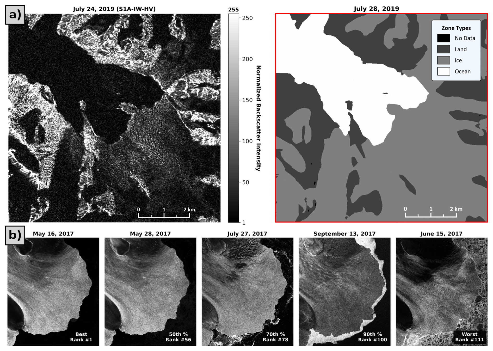
Figure 4 (a) Preprocessed SAR and zone label glacier-style training data image pair rasterized to the glacier's RGI box extent at 10 m spatial resolution. The pictured SAR image, obtained by the Sentinel-1A satellite on 24 July 2019, in IW mode with HV cross-polarization, is four days before the date in which Kochtitzky et al. (2022b) mapped the terminus position from a Landsat-8 optical image at this glacier (28 July 2019). (b) A series of preprocessed SAR images at Austfonna Basin 3 demonstrating the relative image quality ranking system per RGI basin per year, which helps select reference images for supporting the multi-temporal segmentation model. The best, 50–70–90th percentile, and worst images are shown left to right, with their image date and rank number provided among the 111 available SAR images at Austfonna Basin 3 in 2017. Spectral signatures can vary temporally under the applied normalization due to changes in the glacier's velocity (best and 50th % images), presence of sea ice or mélange (90th % and worst images), as well as surface melt and snowfall.

To preprocess SAR images for training, full Sentinel-1 scenes are cropped to the RGI box geometry and coregistered to the box's reference raster. Due to the spatial footprint of along-orbit acquisitions, a coregistered image may only partially cover the box's extent (see Fig. S1a in the Supplement); in some cases, incomplete coverage is restored by mosaicking consecutive along-orbit images. After merging, all coregistered images are normalized with a percentile-based scaling, where pixel intensities are clipped to the 5th and 95th percentiles of the image's valid data distribution and linearly rescaled to an integer range of 1–255, with the nodata value set to 0. For quality control, any lingering partial cover images with less than 99 % data coverage are removed if the corresponding reference 2019 polygons are not fully contained by valid data pixels. The accompanying zone label image is produced by clipping each of the zone layers with the RGI box, rasterizing the clips onto the reference raster, and burning the SAR image's nodata pixels onto the raster.

Before generating predictions, all SAR scenes from 2015–2024 are preprocessed with the same cropping, coregistration, merging, and normalization workflow as applied to the training data. However, the handling of partial coverage images is modified to retain images that may still provide useful frontal information. Like the training data, images with less than 99 % valid data coverage are identified; from the filtered set, images under 75 % overall coverage or less than 90 % coverage within the rasterized postprocessing geometry are removed (see Sect. S1.2 in the Supplement for RGI box postprocessing geometry). To support model segmentation stability during training and when generating predictions, the multi-temporal input sequence is complemented with a fixed land mask, as we assume land to be constant throughout the study period. Additionally, we implement a relative image quality ranking scheme for each RGI basin and year, to identify the most suitable reference images for the segmentation model (Fig. 4b). For each SAR image, pixel intensities are sampled over common ocean and ice masks derived by rasterizing the regional zone label (i.e. the training label) geometry onto the RGI box reference raster. While the masks are static and glacier termini evolve throughout the study period, retrospective analysis using the minimum and maximum observed monthly glacier extents (see Sect. 3.1.5) demonstrates that frontal displacement is small relative to glacier outlet area. Across all glaciers, the median maximum disagreement between the static ice mask and the observed glacier extents over the study period is 2.7 % (95th percentile: 11.6 %) of the outlet area. Similarly, the median glacier area variability between the minimum and maximum observed monthly extents is 3.9 % (95th percentile: 17.6 %) of the outlet area. These results support the use of static ice and ocean masks as a close approximation of the regions sampled for reference image quality ranking. Seven statistical metrics describing ice-ocean separability and noise characteristics are computed from the sampled backscatter values: (1) a normalized percentile overlap metric, (2) the median intensity contrast, (3) the mean ice-to-ocean intensity ratio, (4) the ice-ocean Shannon entropy difference (Shannon, 1948), (5) the ocean dark-pixel fraction, (6) the ice-to-ocean coefficient of variation ratio, and (7) a Kolmogorov–Smirnov contrast metric (Kolmogorov, 1933). The metrics are standardized and combined using a principal component analysis, with the first component used as a composite image quality score. The composite score is sorted such that higher scores correspond to stronger ice–ocean contrast, and images are ranked accordingly within each RGI-ID per year. Detailed definitions of the individual image quality metrics are provided in the supplementary material (Sect. S1.1). The described SAR image preprocessing is the same for images acquired with IW and EW mode, except during image coregistration the 40 m native spatial resolution of EW images (only used for KV) is upscaled to match the native 10 m resolution of IW acquisitions. In total, we preprocess, rank, and output model predictions for 203 294 images across all RGI boxes from 2015–2024.

3.1.5 Monthly prediction averaging and glacier domain polygons

Using the segmentation model's postprocessed predictions (see supplement Sect. S1.2 for postprocessing method), ice front positions are averaged to a monthly mean. Postprocessed predictions are first constrained to only consider connected ice pixel clusters that intersect the fluxgate geometry (see Sect. 3.2.1 for fluxgates). These connected ice clusters are then converted into signed distance transform (SDT) fields (Felzenszwalb and Huttenlocher, 2012), denoting the closest Euclidean distance to the ice cluster boundary per pixel. The SDT fields are stacked using all available predictions per month and aggregated using the mean distance value per pixel. The monthly mean SDTs are subsequently reclassified into ice, ocean, and land classes by thresholding the ice-ocean boundary along the zero-distance contour and preserving the fixed land pixels from the postprocessed prediction. The SDT approach produces a geometrically averaged ice front position that is spatially coherent, temporally stable, and robust to prediction variability. Given 147 RGI boxes and 120 months in the study period, there are 17 640 possible monthly front positions, of which we produce 16 704 due to the prefiltered outliers during the postprocessing.

To extract calving front lines, an SDT field is calculated for each monthly mean zone prediction, then the zero contours of fluxgate-connected ice clusters are extracted and smoothed with an adaptive window Savitzky-Golay filter (Savitzky and Golay, 1964) based on ice front length to reduce pixel discretization while preserving terminus geometry. SDT values for N/A and land pixels are masked, resulting in contours that only correspond to the ice-ocean interface (Fig. 5). For quality control, the resulting front lines are manually checked for outliers across all glaciers, using the preprocessed SAR imagery from matching months as a reference comparison for suspect ice fronts. Front lines of apparent surge events are rigorously inspected for relative scale and temporal accuracy. Overall, 1057 fronts are manually removed, leaving a total of 15 647 valid monthly ice front predictions or 88.7 % temporal coverage of all possible fronts. The missing 11.3 % of possible front predictions is due to a combination of insufficient temporal coverage of IW mode SAR imagery, automated postprocessing filters of the daily predictions, and the manual outlier inspection of monthly averaged ice fronts.

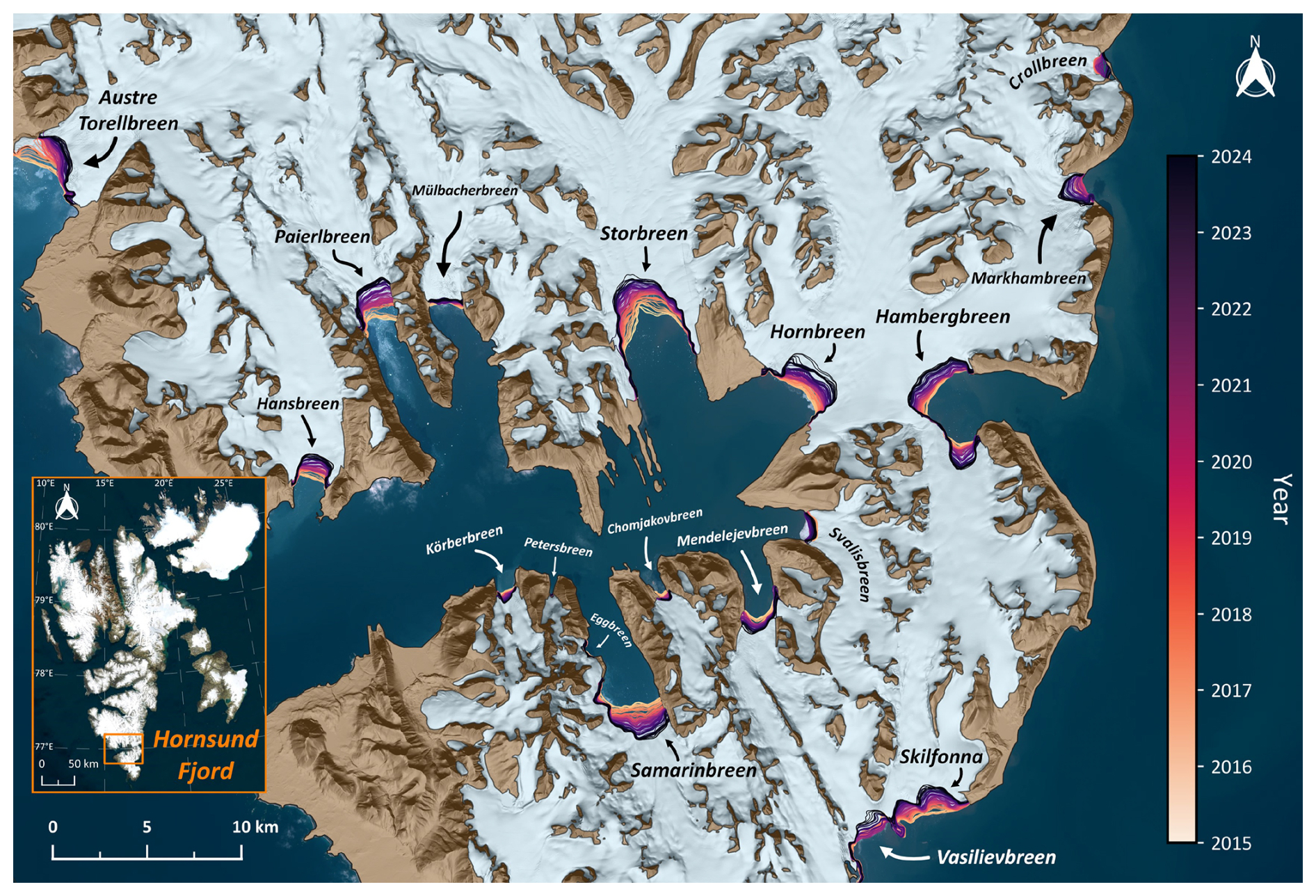
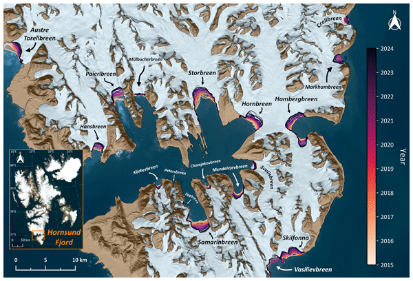
Figure 5 Geographic map of the Hornsund Fjord and peripheral tidewater glaciers in South Spitsbergen (SS), showing a spatial distribution and variability of monthly-averaged terminus position segmentation predictions from 2015–2024 across 18 glaciers (2050 calving fronts). Background of the inset map is provided by the Bing Satellite ©, ocean imagery is cropped from a Sentinel-2 scene obtained on 18 August 2019, and the topography of ice and land is given by a hill shade generated from a Svalbard DEM (Geyman et al., 2021). Extent of ice, ocean, and land reflects the updated regional zone labels, originally derived from RGI version 6.

After manual front filtering, we generate polygons of the glacier domain from the remaining monthly predictions to estimate the ice area by only retaining features that intersect the glacier's fluxgate geometry. Polygon boundaries are smoothed using buffer-based geometric smoothing and simplification to produce a more realistic front morphology and reduce the stair-stepping artifacts inherent to raster-derived outlines. Smoothed polygons are clipped with the regional land zone label to clean fragments overlapping land area. As the polygon area always extends above and below the fluxgate, the polygons are subsequently split with the fluxgate line geometries, and glacier orientation points are used to determine which split polygon corresponds to the glacier domain (see Sect. 3.2.1 for orientation points). If multiple valid polygons exist in the glacier domain, usually due to retreat and separation of ice into distinct glacial trunks, the polygons are merged.

3.1.6 Frontal area change and uncertainty

To fully resolve the frontal area change component, we calculate the width-averaged frontal displacement rates, define the width of all monthly-averaged predicted ice fronts, and estimate cross-sectional areas at the fluxgate. Recalling the frontal area change component in Eq. (1):

$$\begin{array}{}\text{(2)}& A_{\mathrm{front}}=S_{\mathrm{g}}{\displaystyle \frac{W_{\mathrm{f}}}{W_{\mathrm{g}}}}\dot{L}.\end{array}$$

The frontal displacement rate term $\dot{\left(L\right)}$ is defined such that:

$$\begin{array}{}\text{(2a)}& \dot{L}={\displaystyle \frac{\mathrm{\Delta }A}{{\stackrel{\mathrm{‾}}{W}}_{\mathrm{f}}\mathrm{\Delta }t}}\end{array}$$

where ΔA is the planimetric area change between consecutive glacier domain polygons, ${\stackrel{\mathrm{‾}}{W}}_{\mathrm{f}}$ is the averaged ice front width from both time steps, and Δt is the elapsed time given in months. The ice front width is approximated by summing the length of all zero contours per reference front line, yielding the terminus length for each month. The cross-sectional area (S_g) is computed by summing the discrete ice column areas for all flux segments across the fluxgate (see Sect. 3.2.4). The ratio $W_{\mathrm{f}}{W}_{\mathrm{g}}^{-\mathrm{1}}$ is a geometric width-scaling factor that accounts for differences between the fluxgate and frontal widths by rescaling the fluxgate cross-sectional area so that the area change is expressed in terms of frontal geometry; the front and fluxgate widths from the second time step are used.

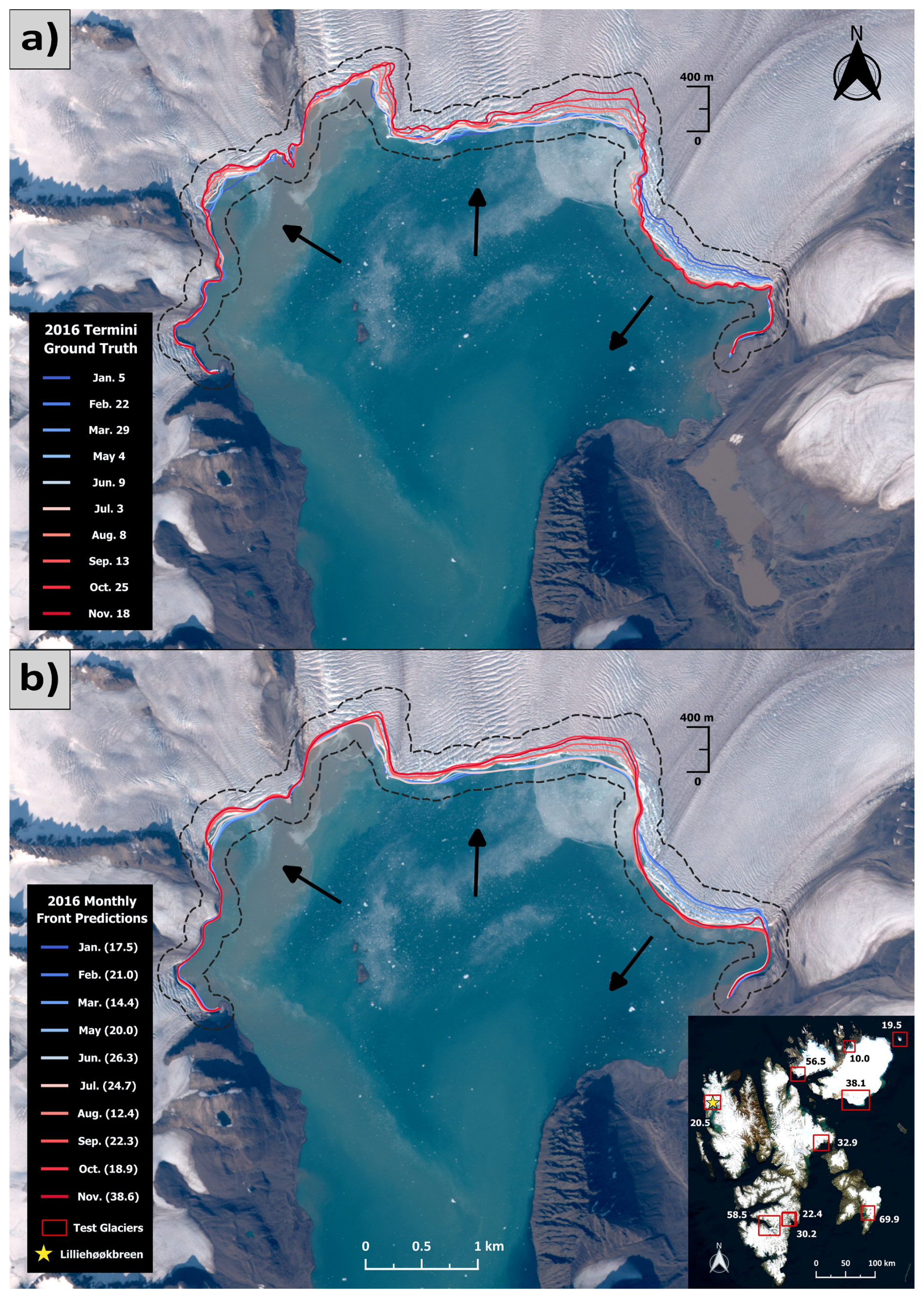
Figure 6 Background for both panels is a Sentinel-2 image obtained on 2 August 2016. (a) The 10 manually mapped terminus positions from SAR images at Lilliehøøkbreen over the evaluation period in 2016. Arrows indicate a retreat over the year on the left and middle thirds of the glacier and a frontal advance on the right third. The dashed black line provides a consistent visual reference for comparing the panels. (b) The 10 monthly-averaged ice front model predictions, forming pairs with the ground truth positions by the corresponding month. The model captures the observed contrasting retreat/advance pattern during 2016. The width-averaged spatial uncertainty per pair is provided in meters in the legend. The inset map shows the geographic location of all glaciers included in the frontal uncertainty analysis, with the map background given by the Bing Satellite ©. Mean pair spatial uncertainties are annotated in meters on the inset map per testing glacier.

Uncertainty in the frontal displacement rate (${\mathit{\sigma }}_{\dot{L}}$) is estimated by comparing manually delineated and model-predicted glacier domain polygons from the same month (Fig. 6), across a geographically, geometrically, and behaviorally diverse subset of 10 tidewater glaciers (Table S1 in the Supplement). The glaciers were manually selected to be representative of the various types of glaciers found in Svalbard (Sect. S1.3), including factors such as variable calving front length, observed surge behavior, complex and simple frontal geometry, and glacier flow type (fjord or ice cap style). While 10 ground truth ice fronts are manually digitized per glacier across the evaluation period in 2016 (100 total), comparisons are only made for months with an accompanying model-predicted polygon, leaving 89 polygon pairs for evaluation. To estimate the uncertainty per pair (σ_front,i), the absolute area disagreement between the manually digitized and predicted polygon is normalized by the ground truth terminus length (W_manual), giving a spatial uncertainty that reflects geometric complexity of the ice front:

$$\begin{array}{}\text{(3a)}& {\mathit{\sigma }}_{\mathrm{front},i}={\displaystyle \frac{\left|\mathrm{\Delta }{A}_{\text{pred-manual}}\right|}{W_{\mathrm{manual}}}}.\end{array}$$

We define a regional uncertainty (${\stackrel{\mathrm{‾}}{\mathit{\sigma }}}_{\mathrm{front}}$) by taking the mean of the per-glacier mean uncertainties, representing a typical frontal displacement uncertainty applicable to glaciers lacking manual validation. The mean regional frontal uncertainty is 38.1 m. The regional spatial uncertainty is converted to a frontal displacement rate uncertainty by dividing with the time separation between consecutive polygon predictions:

$$\begin{array}{}\text{(3b)}& {\mathit{\sigma }}_{\dot{L}}={\displaystyle \frac{{\stackrel{\mathrm{‾}}{\mathit{\sigma }}}_{\mathrm{front}}}{\mathrm{\Delta }t}}.\end{array}$$

Consistent with the calculation of the cross-sectional area, the uncertainty (${\mathit{\sigma }}_{S_{\mathrm{g}}}$) is estimated by summing the discrete ice column area errors for all flux segments across the fluxgate. The frontal area change uncertainty (${\mathit{\sigma }}_{A_{\mathrm{front}}}$) is then given by standard error propagation of products, assuming independent uncertainties:

$$\begin{array}{}\text{(4)}& {\mathit{\sigma }}_{A_{\mathrm{front}}}={\displaystyle \frac{W_{\mathrm{f}}}{W_{\mathrm{g}}}}\sqrt{{\left(\dot{L}{\mathit{\sigma }}_{S_{\mathrm{g}}}\right)}^{\mathrm{2}}+{\left(S_{\mathrm{g}}{\mathit{\sigma }}_{\dot{L}}\right)}^{\mathrm{2}}}.\end{array}$$

As the fluxgate width is fixed to finite points along the gate (see Sect. 3.2.1), the width of the gate (W_g) has no uncertainty. Likewise, following the approach of Minowa et al. (2021), uncertainty in W_f has a negligible contribution (1.7 %) compared to the other propagated components in Eq. (4) and is therefore not considered.

3.2 Ice discharge

3.2.1 Fluxgates, points, and flow orientation

To calculate ice discharge, we first describe the placement of fluxgates, the sampling scheme of terms composing the discharge, and define an orientation of ice flow towards the ocean. Fluxgates are manually digitized, placing the gate behind the most retreated terminus extent over the full time series for a given glacier. However, we do not place the gate too far upstream of this extent, as to not introduce unnecessary ice area into the glacier's domain, which is important for minimizing the uncertainty in the climatic mass balance correction (see Sect. 3.3). If the ice thickness coverage is sparse around the retreated extent, the gate is moved further upstream where complete thickness coverage exists. A gate's endpoints are often bounded to the regional land zone label to facilitate splitting of the monthly ice area polygons and extraction of the ice area within the domain (see Sect. 3.1.5). However, some glacier domains are adjacent to each other and there is no land label within their RGI boxes; in these cases, we extend the endpoints across both glaciers' laterally shared ice boundary, ensuring that all ice polygons can be split with the gate geometry. Some RGI basins contain multiple gates to partition separate tidewater glaciers within the box, with the final discharge being summed. As the Svalbard archipelago is not characterized by ice shelves and only small areas near the glacier termini may be floating, we assume the upstream placements of the fluxgates are positioned over grounded ice.

Along a fluxgate, we interpolate evenly spaced fluxgate points every 100 m, with the flux points serving as the sampling geometries for ice discharge computation. The points are generated in the WGS84 NSIDC Sea Ice Polar Stereographic North projection (EPSG 3413) for compatibility with the ice velocity and thickness datasets. An ice discharge is computed for each flux point contained within the regional ice zone label. To integrate point sampled values across the width of the fluxgate, a flux segment or “ice column” is defined by the midpoints between consecutive flux points. On both sides of a flux point (p), there are two midpoints (m₁, m₂) that are some distance from the flux point, with the sum of these distances (w₁, w₂) defining the width of the flux segment (w_seg):

$$\begin{array}{}\text{(5a)}& {\displaystyle }& {\displaystyle }\mathit{p}=\left(x_p,y_p\right){\mathit{m}}_{\mathrm{1}}=\left(x_{\mathrm{1}},y_{\mathrm{1}}\right){\mathit{m}}_{\mathrm{2}}=\left(x_{\mathrm{2}},y_{\mathrm{2}}\right)\text{(5b)}& {\displaystyle }& {\displaystyle }{w}_i=\sqrt{{\left(x_p-x_i\right)}^{\mathrm{2}}+{\left(y_p-y_i\right)}^{\mathrm{2}}},i=\mathrm{1},\mathrm{2}\text{(5c)}& {\displaystyle }& {\displaystyle }{w}_{\mathrm{seg}}=w_{\mathrm{1}}+w_{\mathrm{2}}.\end{array}$$

To spatially orient a fluxgate relative to ice flow direction through the gate, an orientation point is manually placed on the glacier, also behind the most retreated terminus extent. There are two types of orientation point placements, which depend on the glacier's morphologic flow style; the point for most fjord-style glaciers is set within the glacier domain, downstream of the fluxgate (orientation = 0, Fig. 7a), however, for ice cap- and island-style glaciers with unconstrained flow, the orientation point is placed upstream of the fluxgate (orientation = 1, Fig. 7b).

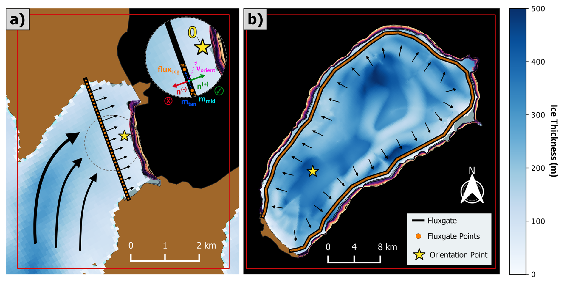
Figure 7 Example of the fluxgates, flux points, and orientation point geometry styles. The fluxgate and orientation point are placed behind the most retreated terminus position. Ice thickness, velocity, and surface elevation change data are point-sampled at the flux points. Red outlines are the glaciers RGI boxes. Thickness data are derived from Fürst et al. (2018a). (a) Fjord-style morphology where the orientation point equals 0 and is placed within the glacier domain, with ice flow towards the point. Large arrows represent possible flow directions to the fluxgate and small arrows show normal flow vectors perpendicular to flux segments. The pop-out schematic (within the dashed grey circle) illustrates an example of the normal orientation selection process, showing the accepted (green check) and rejected (red x) candidate normal directions for a single flux segment. (b) The Kvitøyjøkulen ice cap representative of an island-style glacier with morphologically unconstrained flow and an orientation point value of 1; ice flows away from the orientation point and toward the terminus (arrows).

The primary purpose of the orientation point is to define a consistent normal flow direction for each flux segment. To compute ice discharge through a flux segment, the sampled ice surface velocity is projected onto the selected segment normal. Because each flux segment has two possible perpendicular directions, the downstream flow direction is ambiguous. The orientation point resolves this ambiguity by consistently identifying the downstream side of the fluxgate. For each flux segment, the local tangent vector (m_tan) is computed as the difference between the segment's midpoints. The tangent angle (θ_tan) is then calculated from this vector, and two normals (n⁽⁺⁾, n⁽⁻⁾) are defined:

$$\begin{array}{}\text{(6a)}& {\displaystyle }& {\displaystyle }{\mathit{m}}_{\tan }={\mathit{m}}_{\mathrm{2}}-{\mathit{m}}_{\mathrm{1}}\text{(6b)}& {\displaystyle }& {\displaystyle }{\mathit{\theta }}_{\tan }=\mathrm{atan}\mathrm{2}\left(m_{\tan ,y},m_{\tan ,x}\right)\text{(6c)}& {\displaystyle }& {\displaystyle }{\mathit{n}}^{(+)}=\left(\begin{array}{c}-\sin {\mathit{\theta }}_{\tan }\\ \cos {\mathit{\theta }}_{\tan }\end{array}\right),{\mathit{n}}^{(-)}=\left(\begin{array}{c}\sin {\mathit{\theta }}_{\tan }\\ -\cos {\mathit{\theta }}_{\tan }\end{array}\right).\end{array}$$

The orientation point defines an orientation vector (v_orient) between the orientation point (o) and the segment midpoint (m_mid). Depending on the orientation flag, the vector is directed either from the segment midpoint to the orientation point (orientation = 0) or from the orientation point to the segment midpoint (orientation = 1):

$$\begin{array}{}\text{(6d)}& {\displaystyle }& {\displaystyle }\mathit{o}=\left(x_{\mathrm{o}},y_{\mathrm{o}}\right),{\mathit{m}}_{\mathrm{mid}}={\displaystyle \frac{\left({\mathit{m}}_{\mathrm{1}}+{\mathit{m}}_{\mathrm{2}}\right)}{\mathrm{2}}}\text{(6e)}& {\displaystyle }& {\displaystyle }{\mathit{v}}_{\mathrm{orient}}=\left\{\begin{array}{cc}\mathit{o}-{\mathit{m}}_{\mathrm{mid}},& \mathrm{if}\mathrm{orientation}=\mathrm{0}\\ {\mathit{m}}_{\mathrm{mid}}-\mathit{o},& \mathrm{if}\mathrm{orientation}=\mathrm{1}\end{array}\right..\end{array}$$

The candidate normal (n) whose direction is most closely aligned with the orientation vector is then selected:

$$\begin{array}{}\text{(6f)}& \mathit{n}=\begin{array}{c}\mathrm{argmax}\\ {\mathit{n}}^{(\pm )}\end{array}\left({\mathit{n}}^{(\pm )}\cdot {\mathit{v}}_{\mathrm{orient}}\right).\end{array}$$

This process ensures a consistent sign convention for ice discharge across all flux segments because the orientation point is always downstream (orientation = 0) or upstream (orientation = 1) of the fluxgate's local tangent vectors.

3.2.2 Ice thickness and surface elevation change

To estimate the ice discharge, ice thickness information is essential. An ice thickness map (H_ref) is generated for Svalbard by differencing the surface reference Copernicus GLO-30 Digital Elevation Model (DEM; European Space Agency and Airbus, 2022) from the ice-free bedrock topography of Svalbard (Fürst et al., 2017, 2018a, b). Similarly, ice thickness uncertainties are obtained from the error map provided in Fürst et al. (2018a). If a flux point contained within the regional ice zone label is missing thickness or error measurements, values are linearly interpolated across the flux points. We sample ice surface elevation change rates from a $\partial H\partial t^{-\mathrm{1}}$ field derived by DEM differencing between 2013–2018 (Malz et al., 2021). Two island glaciers in northeast Svalbard – Kvitøyjøkulen and Storøyjøkulen – are missing surface elevation change data, which is filled with a glacier-specific constant rate from the period January 2015–2020 for all flux points (Hugonnet et al., 2021). There are 11 additional glaciers with partial elevation change data due to radar shadow, whose missing flux points are filled with the mean rate of available point measurements. Ten of these glaciers are only missing data at one or two flux points, with the final glacier of the subset missing a larger proportion of points because of poor scene coverage in the DEM differencing. We assume the thickness map reference date to be 31 December 2013, coincident with the survey period of the Copernicus DEM (January 2011–July 2015). Therefore, to estimate time-corrected ice thicknesses (H) at each monthly time step, the reference ice thickness (H_ref) is linearly adjusted using the sampled ice surface elevation change rates ($\partial H\partial t^{-\mathrm{1}}$) such that:

$$\begin{array}{}\text{(7)}& H=H_{\mathrm{ref}}+{\displaystyle \frac{\partial H}{\partial t}}\mathrm{\Delta }t\end{array}$$

where Δt is the time difference between the ice thickness reference date and the target month's midpoint in days.

3.2.3 Ice velocity

The Inter-mission Time Series of Land Ice Velocity and Elevation (ITS_LIVE) catalog provides tiled ice velocity datacubes (Gardner et al., 2025; ITS_LIVE team, 2026). We use all available image-pair velocity maps within a temporal baseline of one month (≤32 d) from 2015–2024, including pairs from Sentinel-1 A/B, Sentinel-2 A/B, and Landsat 8/9. For a fluxgate and its flux points, vector velocities (v_x, v_y) and errors (${\mathit{\sigma }}_{v_x}$, ${\mathit{\sigma }}_{v_y}$) are sampled from all overlapping ITS_LIVE tiles and the velocity magnitude (v) and uncertainty (σ_v) are derived:

$$\begin{array}{}\text{(8)}& {\displaystyle }& {\displaystyle }v=\sqrt{v_x^{\mathrm{2}}+v_y^{\mathrm{2}}}\text{(9)}& {\displaystyle }& {\displaystyle }{\mathit{\sigma }}_v=\sqrt{{\left({\displaystyle \frac{v_x}{v}}{\mathit{\sigma }}_{v_x}\right)}^{\mathrm{2}}+{\left({\displaystyle \frac{v_y}{v}}{\mathit{\sigma }}_{v_y}\right)}^{\mathrm{2}}}.\end{array}$$

Ice flow direction (θ_v) is computed from the vector velocity components and defined as a bearing measured clockwise from north, constrained to [0, 360°). The uncertainty in flow direction (${\mathit{\sigma }}_{{\mathit{\theta }}_v}$) is estimated by propagating uncertainties in the velocity components; measurements with an angular uncertainty exceeding 180° are discarded to remove poorly constrained flow directions:

$$\begin{array}{}\text{(10)}& {\displaystyle }& {\displaystyle }{\mathit{\theta }}_v=\left(\mathrm{90}\mathit{°}-\mathrm{atan}\mathrm{2}\left(v_y,v_x\right)\right)\mathrm{mod}\mathrm{360}\mathit{°}\text{(11)}& {\displaystyle }& {\displaystyle }{\mathit{\sigma }}_{{\mathit{\theta }}_v}=\sqrt{{\displaystyle \frac{v_y^{\mathrm{2}}{{\mathit{\sigma }}_{v_x}}^{\mathrm{2}}+v_x^{\mathrm{2}}{{\mathit{\sigma }}_{v_y}}^{\mathrm{2}}}{{\left(v_x^{\mathrm{2}}+v_y^{\mathrm{2}}\right)}^{\mathrm{2}}}}}.\end{array}$$

To produce a monthly velocity magnitude, flow direction, and associated uncertainties, observations are aggregated in two stages: daily, then monthly. In the sampled time series, a day may contain multiple velocity measurements due to overlapping satellite acquisitions. Therefore, to prevent the monthly average from being biased to a skewed daily distribution, all measurements are first averaged on a per day resolution. Daily velocity magnitudes and their uncertainties are computed as means, and monthly values are then derived from the mean of the daily means.

Because flow direction is an angular variable, directional averaging is performed using circular statistics. Daily mean flow direction (θ_d) is calculated by averaging the sine and cosine components of the flow directions and deriving the mean angle from the resulting mean vector. Uncertainty in the daily mean flow direction (${\mathit{\sigma }}_{{\mathit{\theta }}_{\mathrm{d}}}$) is propagated from the individual angular uncertainties, assuming independent measurements:

$$\begin{array}{}\text{(12)}& {\displaystyle }& {\displaystyle }{\mathit{\theta }}_{\mathrm{d}}=\mathrm{atan}\mathrm{2}\left({\displaystyle \frac{\mathrm{1}}{N_{\mathrm{d}}}}\sum _{i=\mathrm{1}}^{N_{\mathrm{d}}}\sin {\mathit{\theta }}_{v,i},{\displaystyle \frac{\mathrm{1}}{N_{\mathrm{d}}}}\sum _{i=\mathrm{1}}^{N_{\mathrm{d}}}\cos {\mathit{\theta }}_{v,i}\right)\text{(13a)}& {\displaystyle }& {\displaystyle }{\mathit{\sigma }}_{{\mathit{\theta }}_{\mathrm{d}}}=\sqrt{{\displaystyle \frac{\mathrm{1}}{N_{\mathrm{d}}}}\sum _{i=\mathrm{1}}^{N_{\mathrm{d}}}{\mathit{\sigma }}_{{\mathit{\theta }}_{v,i}}^{\mathrm{2}}}\end{array}$$

where N_d denotes the number of velocity observations available on day d. Monthly flow direction (θ_m) is computed as the circular mean of the daily mean flow directions, given by:

$$\begin{array}{}\text{(14)}& {\mathit{\theta }}_{\mathrm{m}}=\mathrm{atan}\mathrm{2}\left({\displaystyle \frac{\mathrm{1}}{N_{\mathrm{m}}}}\sum _{d=\mathrm{1}}^{N_{\mathrm{m}}}\sin {\mathit{\theta }}_{\mathrm{d}},{\displaystyle \frac{\mathrm{1}}{N_{\mathrm{m}}}}\sum _{d=\mathrm{1}}^{N_{\mathrm{m}}}\cos {\mathit{\theta }}_{\mathrm{d}}\right)\end{array}$$

where N_m is the number of daily mean flow directions available in month m. The monthly flow uncertainty is defined using two alternative approaches: (1) when sufficient daily observations are available and the resulting angular dispersion is physically meaningful (i.e. ≤180°), uncertainty is quantified using the circular standard deviation, otherwise, (2) the monthly uncertainty is defined as the mean of the propagated daily uncertainties. This fallback is applied for months with sparse velocity observations or highly variable daily flow directions, both of which are rare. The circular standard deviation (${\mathit{\sigma }}_{{\mathit{\theta }}_{\mathrm{m}}}^{\mathrm{circ}}$) is calculated from the mean resultant length (R_m):

$$\begin{array}{}\text{(13b)}& {\displaystyle }& {\displaystyle }{R}_{\mathrm{m}}=\sqrt{{\left({\displaystyle \frac{\mathrm{1}}{N_{\mathrm{m}}}}\sum _{d=\mathrm{1}}^{N_{\mathrm{m}}}\cos {\mathit{\theta }}_{\mathrm{d}}\right)}^{\mathrm{2}}+{\left({\displaystyle \frac{\mathrm{1}}{N_{\mathrm{m}}}}\sum _{d=\mathrm{1}}^{N_{\mathrm{m}}}\sin {\mathit{\theta }}_{\mathrm{d}}\right)}^{\mathrm{2}}}\text{(13c)}& {\displaystyle }& {\displaystyle }{\mathit{\sigma }}_{{\mathit{\theta }}_{\mathrm{m}}}^{\mathrm{circ}}=\sqrt{-\mathrm{2}\ln \left(R_{\mathrm{m}}\right)}.\end{array}$$

The final monthly flow-direction uncertainty (${\mathit{\sigma }}_{{\mathit{\theta }}_{\mathrm{m}}}$) is then defined as:

$$\begin{array}{}\text{(15)}& {\mathit{\sigma }}_{{\mathit{\theta }}_{\mathrm{m}}}=\left\{\begin{array}{ll}{\mathit{\sigma }}_{{\mathit{\theta }}_{\mathrm{m}}}^{\mathrm{circ}},& \mathrm{if}{N}_{\mathrm{m}}>\mathrm{1}\mathrm{and}{\mathit{\sigma }}_{{\mathit{\theta }}_{\mathrm{m}}}^{\mathrm{circ}}\le \mathit{\pi }\\ \frac{\mathrm{1}}{N_{\mathrm{m}}}\sum _{d=\mathrm{1}}^{N_{\mathrm{m}}}{\mathit{\sigma }}_{{\mathit{\theta }}_{\mathrm{d}}},& \mathrm{otherwise}\end{array}\right..\end{array}$$

For additional details on deriving the complete monthly ice velocity time series, including quality control filters and subsequent reconstruction, see the supplementary material (Sect. S2).

3.2.4 Ice discharge and uncertainty equations

In the frontal ablation equation, ice discharge (D) is calculated as the product of ice velocity (v) and thickness (H). We assume a bulk ice density (p_ice) of 900 kg m⁻³ to account for the presence of air bubbles and porosity within glacier ice, and a sliding coefficient (γ) of 0.95 (Cuffey and Paterson, 2010), to account for depth-averaged velocity ($\stackrel{\mathrm{‾}}{v}$), where $\stackrel{\mathrm{‾}}{v}=v\mathit{\gamma }$. Because discharge is calculated at discrete points and integrated over finite flux segments of length w_seg, the discharge is summed across all segments (N_seg):

$$\begin{array}{}\text{(16)}& D=p_{\mathrm{ice}}\sum _{n=\mathrm{1}}^{N_{\mathrm{seg}}}\stackrel{\mathrm{‾}}{v}H{w}_{\mathrm{seg}}\cos \left(\mathrm{\Delta }\mathit{\theta }\right).\end{array}$$

Equation (16) approximates a glacier's total monthly ice discharge across the fluxgate, where the cosine term accounts for the angular difference (Δθ) between the monthly ice flow direction and the fluxgate normal. The segment-wise uncertainty in ice discharge (σ_Dseg) is also estimated through standard error propagation, assuming independent uncertainties of the discharge components:

$$\begin{array}{}\text{(17)}& {\mathit{\sigma }}_{\mathrm{Dseg}}=\sqrt{{\left({\displaystyle \frac{\partial D}{\partial H}}{\mathit{\sigma }}_H\right)}^{\mathrm{2}}+{\left({\displaystyle \frac{\partial D}{\partial v}}{\mathit{\sigma }}_v\right)}^{\mathrm{2}}+{\left({\displaystyle \frac{\partial D}{\partial \mathrm{\Delta }\mathit{\theta }}}{\mathit{\sigma }}_{\mathrm{\Delta }\mathit{\theta }}\right)}^{\mathrm{2}}}.\end{array}$$

Uncertainty in the flux segment width is not propagated, as we assume a constant segment width with no associated uncertainty. Evaluating the partial derivatives in Eq. (17), summing the segment uncertainties, and multiplying by the ice density yields the discharge uncertainty (σ_D) equation:

$${\mathit{\sigma }}_{\mathrm{D}}=p_{\mathrm{ice}}\sum _{n=\mathrm{1}}^{N_{\mathrm{seg}}}{w}_{\mathrm{seg}}$$

$$\begin{array}{}\text{(17a)}& \sqrt{{\left(\stackrel{\mathrm{‾}}{v}\cos \left(\mathrm{\Delta }\mathit{\theta }\right){\mathit{\sigma }}_H\right)}^{\mathrm{2}}+{\left(H\cos \left(\mathrm{\Delta }\mathit{\theta }\right){\mathit{\sigma }}_v\right)}^{\mathrm{2}}+{\left(H\stackrel{\mathrm{‾}}{v}\sin \left(\mathrm{\Delta }\mathit{\theta }\right)\cdot {\mathit{\sigma }}_{\mathrm{\Delta }\mathit{\theta }}\right)}^{\mathrm{2}}}.\end{array}$$

3.3 Climatic mass balance

The Modèle Atmosphérique Régional climate model (MAR v3.14) provides CMB estimates over the glacier domains from 2015–2024 (Fettweis and Grailet, 2024; Haacker et al., 2024). The MAR data are daily fields, gridded at 6 km spatial-resolution and forced with ECMWF Global Reanalysis v5 atmospheric data (Hersbach et al., 2020). The CMB is approximated as:

$$\begin{array}{}\text{(18)}& \mathrm{CMB}\sim \mathrm{SF}+\mathrm{RF}-\mathrm{RU}-\mathrm{SU}\end{array}$$

where SF is snowfall, RF is rainfall, RU is run-off of melt and rainwater, and SU is sublimation from snow. To prepare the CMB fields for sampling, the grid is transformed from its native Polar Stereographic (EPSG 3413) projected coordinates to the regional Svalbard UTM projection (EPSG 32633). After defining the regional grid, the daily data are aggregated to a monthly resolution, then linearly reprojected onto the regional grid. For each glacier domain, the area between the fluxgate and calving front, monthly mean CMB estimates are derived using a MAR pixel area-weighted mean, integrated over the monthly ice polygon(s), and converted from mm w.e. to m³ w.e. (Fig. 8).

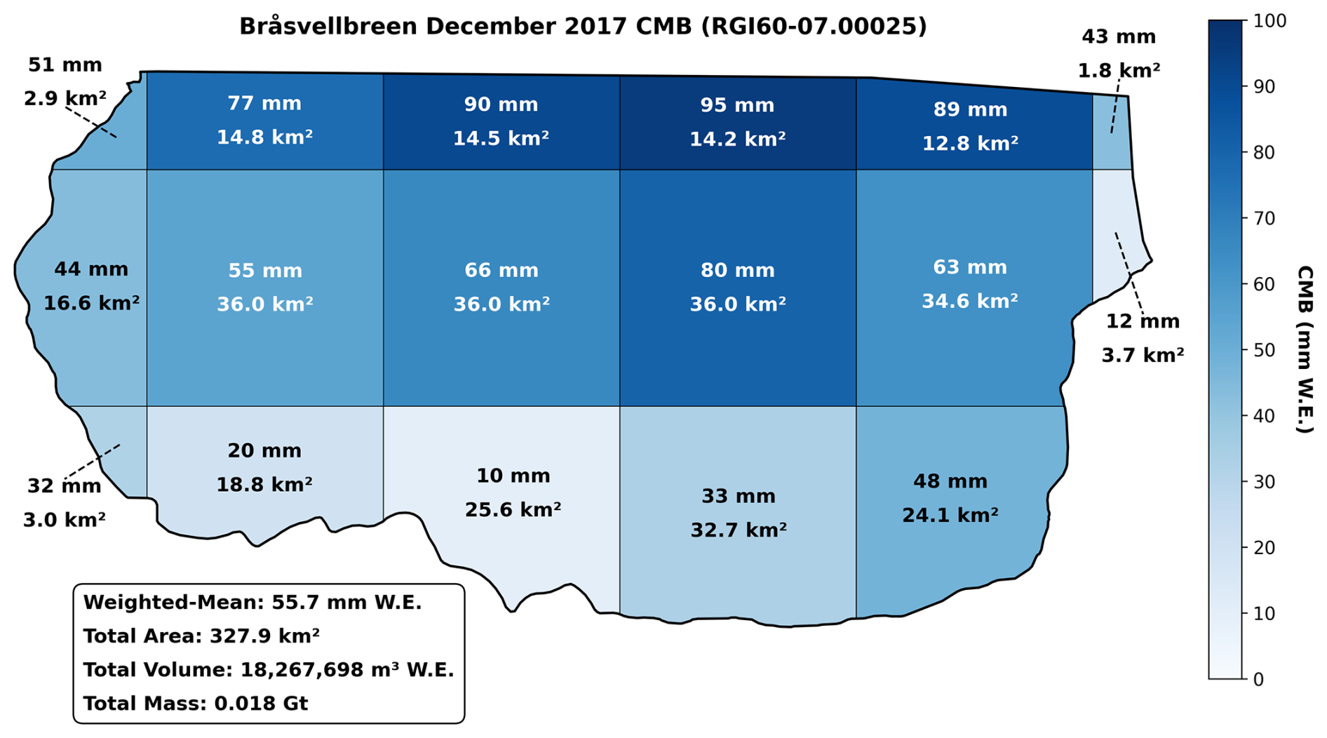
Figure 8 Example of a MAR pixel area-weighted mean CMB, integrated over the glacier domain polygon at Bråsvellbreen in December 2017. A full pixel is 36 km² and partial pixels resulting from clipping to the corresponding monthly ice front polygon or splitting with the fluxgate are weighted accordingly.

3.4 Frontal ablation and uncertainty

With the monthly frontal area change, ice discharge, and CMB time series, the frontal ablation is calculated for all 147 RGI basins. As each glacier must begin with a reference state, frontal ablation is not computed for the first month in a glacier's time series. Therefore, from 15 647 available months, we produce 15 500 monthly frontal ablation estimates in Gt yr⁻¹. Uncertainty in the frontal ablation is defined by standard error propagation of the frontal area change, ice discharge, and CMB uncertainty components:

$$\begin{array}{}\text{(19)}& {\mathit{\sigma }}_{A_{\mathrm{f}}}=\sqrt{{\left({\mathit{\sigma }}_{A_{\mathrm{front}}}\right)}^{\mathrm{2}}+{\left({\mathit{\sigma }}_{\mathrm{D}}\right)}^{\mathrm{2}}+{\left({\mathit{\sigma }}_{{\dot{B}}_{\mathrm{f}}}\right)}^{\mathrm{2}}}.\end{array}$$

To account for temporal gaps in a glacier's time series where frontal information is missing, the computed frontal area change for the latter gap-bounding month is linearly interpolated. The associated uncertainty is propagated assuming independent contributions across the gap months, such that the uncertainty assigned to each month scales with $\frac{\mathrm{1}}{\sqrt{n}}$ to conserve total variance, where n is the number of missing months. To leverage the temporally complete, monthly MAR outputs and capture CMB seasonality over the gap interval, a pixel area-weighted mean CMB is computed independently for each gap month using the first available post-gap polygon. While frontal variations are not considered within the gap period, area changes are generally small relative to the glacier domain; across all interpolation gaps, the median relative change between the pre- and post-gap glacier domains was 2.8 %, while the 95th percentile was 10.1 %. This supports the use of a common glacier domain during interpolation, allowing monthly CMB variability to be retained, rather than restricting CMB sampling to months with available frontal geometry. Similarly, as the complete monthly ice discharge time series is independent from frontal geometry, the standard mean discharge is taken over all gap months (see Sect. 3.2.4). With the complete monthly record of ice discharge and CMB, as well as the temporally interpolated frontal area change, the frontal ablation time series is completed with 17 340 monthly measurements. As such, the only temporal gaps remaining are for glaciers whose frontal geometry record begins after January 2015 or ends before December 2024, as we cannot extrapolate frontal information. Although none of the glaciers have a gapless frontal geometry record (i.e. all have interpolated gaps) due to the filtered outliers (see Sects. 3.1.5 and S1.2), 37, 99, and 129 of the 147 glaciers have a non-interpolated monthly frontal ablation temporal coverage of 95 %, 90 %, and 80 %, respectively. Further, the glacier with the worst non-interpolated temporal coverage is the Doktorbreen/Nathorstbreen system (RGI60-07.01474), with 57 of 119 possible months (∼48 %).

As frontal ablation and its associated component values are averaged temporally – annually and a decadal average of the annual rates between 2015–2024 – and aggregated spatially, the propagation of errors follows a standard sequence consistent with the averaging steps performed on the measured quantities. The uncertainty of per-glacier yearly mean rates (${\mathit{\sigma }}_{X,\mathrm{g},y}$) is the root-sum-square (RSS) of monthly uncertainties for a given component (X), normalized by the number (N) of available months (m) for a glacier (g) in the year (y):

$$\begin{array}{}\text{(20a)}& {\mathit{\sigma }}_{X,\mathrm{g},y}={\displaystyle \frac{\mathrm{1}}{N_{\mathrm{m},\mathrm{g},y}}}\sqrt{\sum _{m=\mathrm{1}}^{N_{\mathrm{m},\mathrm{g},y}}{\left({\mathit{\sigma }}_{X,\mathrm{g},y,\mathrm{m}}\right)}^{\mathrm{2}}}.\end{array}$$

Total regional yearly rates across Svalbard, or its subregions, are summed from the per-glacier yearly means. The uncertainty (${\mathit{\sigma }}_{X,y}^{\mathrm{reg}}$) is defined as the RSS of glacier-year uncertainties for component (X), assuming independent errors between glaciers:

$$\begin{array}{}\text{(20b)}& {\mathit{\sigma }}_{X,y}^{\mathrm{reg}}=\sqrt{\sum _{g=\mathrm{1}}^{N_{\mathrm{g},y}}{\left({\mathit{\sigma }}_{X,\mathrm{g},y}\right)}^{\mathrm{2}}}.\end{array}$$

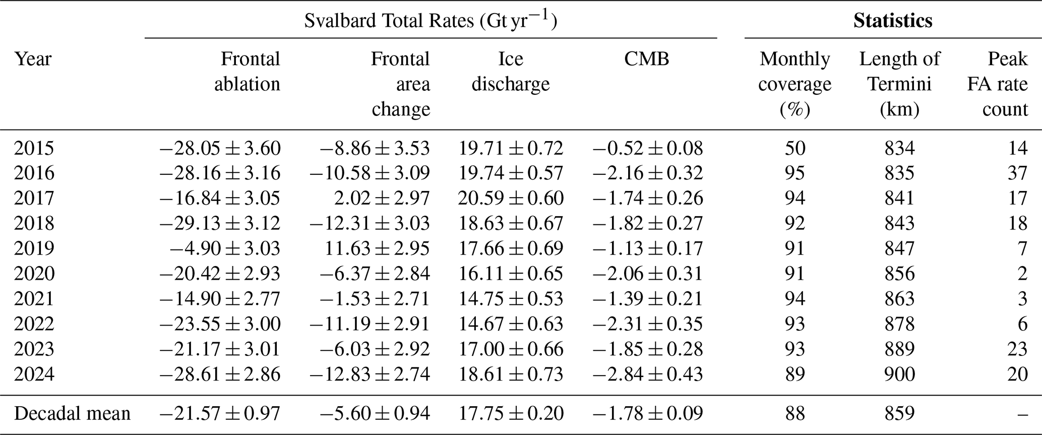
Table 1 Total yearly and decadal frontal ablation, frontal area change, ice discharge, and CMB rates in Gt yr⁻¹, averaged per glacier and summed across all 147 marine terminating glaciers in Svalbard from 2015 to 2024. The monthly coverage is calculated for each year as the percentage of available measurements with frontal information (i.e. non-interpolated) relative to possible measurements for all glaciers. Length of termini is the total summed width of all tidewater glacier fronts. Peak FA rate count is the number of glaciers that had a maximum frontal ablation rate for the given year.

For the reported uncertainties of the regional yearly-averaged CMB component, we apply a 15 % uncertainty, consistent with the established MAR uncertainty for CMB values aggregated across multiple months (Mankoff et al., 2021). Finally, uncertainty in the decadal mean rate (${\mathit{\sigma }}_X^{\mathrm{dec}}$) is estimated by the RSS of regional yearly uncertainties for component (X), normalized by the number of years (i.e. 10):

$$\begin{array}{}\text{(20c)}& {\mathit{\sigma }}_X^{\mathrm{dec}}={\displaystyle \frac{\mathrm{1}}{N_y}}\sqrt{\sum _{y=\mathrm{1}}^{N_y}{\left({\mathit{\sigma }}_{X,y}^{\mathrm{reg}}\right)}^{\mathrm{2}}}.\end{array}$$

The resulting uncertainty represents the propagated measurement uncertainty of the decadal mean and therefore decreases as independent annual estimates are averaged (see Sect. 4.1, Table 1).

4 Results

4.1 Svalbard totals

In total, of 17 493 possible monthly measurements across the 147 marine terminating glaciers defined in the study, we generate 15 500 estimates of frontal ablation, frontal area change, ice discharge, and CMB constrained to model-predicted frontal geometry from 2015–2024 (88 % temporal coverage). An additional 1840 monthly estimates are produced by linearly interpolating temporal gaps of frontal area change within each glacier's time series, resulting in 99 % total temporal coverage (see Sect. 3.4). A yearly rate, averaged across all Svalbard glaciers, is reported for all four components, as well as an annually averaged mean rate over the decade (Table 1), which we hereafter refer to as a decadal rate. Negative frontal ablation, frontal area change, and CMB estimates indicate mass loss. The decadal frontal ablation rate for Svalbard is $-\mathrm{21.57}\pm \mathrm{0.97}$ Gt yr⁻¹ and negative in all years, with a peak yearly rate in 2018 and a low in 2019. Decadal frontal area change is $-\mathrm{5.60}\pm \mathrm{0.94}$ Gt yr⁻¹, with large interannual variability ranging from $-\mathrm{12.83}\pm \mathrm{2.74}$ Gt yr⁻¹ in 2024 to 11.63±2.95 Gt yr⁻¹ in 2019. Eight years are characterized by negative values indicating widespread retreat, juxtaposed to two positive years (2017 and 2019). Comparatively, ice discharge is stable interannually with a peak rate in 2017 (20.59±0.60 Gt yr⁻¹) and a minimum in 2022 (14.67±0.63 Gt yr⁻¹). The decadal ice discharge rate is 17.75±0.20 Gt yr⁻¹ and accounts for ∼82 % of the decadal frontal ablation rate, with the remaining 18 % attributed to mass changes at the terminus (i.e. frontal area change – CMB).

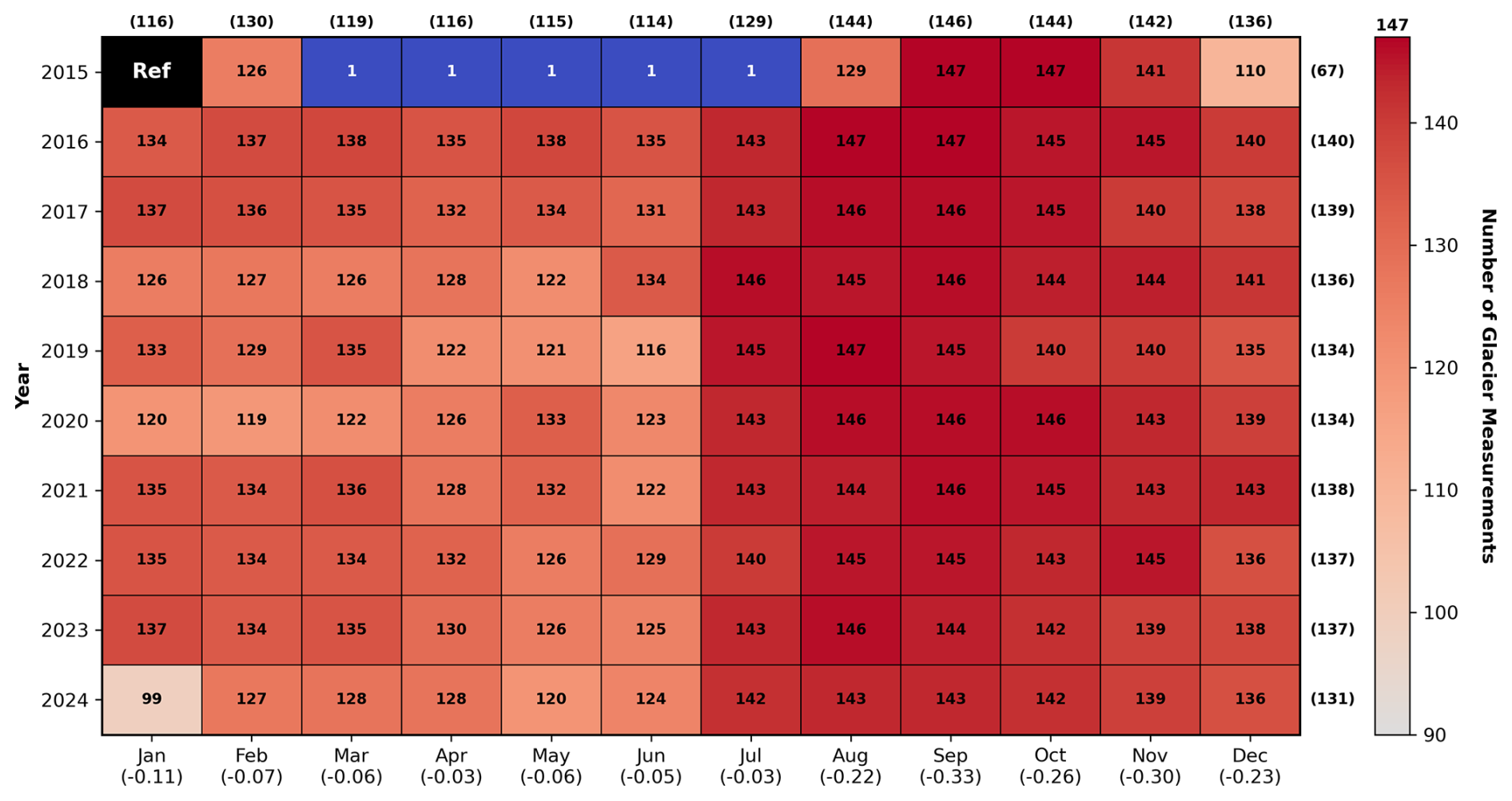
Figure 9 Heat map detailing the number of available per-glacier frontal ablation measurements constrained to frontal geometry (i.e. non-interpolated time series) for all 120 year-month combinations between January 2015 and December 2024. Lower counts are therefore explained by missing monthly frontal information, due to automated and manual outlier filtration. January 2015 is the reference month and thereby has zero frontal ablation measurements. The mean count of available measurements per month is annotated in parentheses on the top axis, and similarly the yearly mean count is provided along the right axis. The mean monthly frontal ablation (Gt yr⁻¹) for all available glacier measurements (interpolated and geometry constrained) is provided below the month axis label.

CMB within the glacier domains is moderately negative in all years, with a mean decadal rate of $-\mathrm{1.78}\pm \mathrm{0.09}$ Gt yr⁻¹, signifying sustained mass loss across the glacier domains due to the climate. Mass loss from the CMB is strongest in 2024 ($-\mathrm{2.84}\pm \mathrm{0.43}$ Gt yr⁻¹) and lowest in 2015 ($-\mathrm{0.52}\pm \mathrm{0.08}$ Gt yr⁻¹). Each year has nearly 90 % temporal monthly measurement coverage averaged across all glaciers, except for 2015 with only 50 % cover because of insufficient Sentinel-1 SAR imagery in the interferometric wide swath (IW) acquisition mode at the beginning of the platform's mission, explaining the lack of spring and summer ice front positions from March to July (Fig. 9). On a per-glacier average, the measurement coverage is more complete in the second half of the years (July–December), suggesting that Svalbard-wide monthly-mean rates are more robust and reliable during these months. Frontal ablation rates are elevated between August and December, with a peak in September (−0.33 Gt yr⁻¹) and a minimum rate in April and July (−0.03 Gt yr⁻¹). The lower data return in the first six months (Fig. 9) is most likely attributed to sea ice and mélange presence, which impacts the segmentation model's predictive performance and consequently results in more outlier predictions than months with ice-free conditions. Another possible explanation, complementary to the impact of ice mélange, is that because the segmentation model is trained on SAR imagery from July and August 2019, there may be a bias towards the ice-free seasonal conditions of those months, potentially affecting the segmentation performance of other months.

The combined length of the tidewater glacier termini increased every year, albeit gradually from 2015 to 2019 (834 to 847 km), then more rapidly from 2019 to 2024 (847 to 900 km) possibly suggesting a destabilization of glacier termini over the 5-year period. Overall, from 2015 to 2024, an additional 66 km of termini (∼8 % increase) were exposed to ocean, and consequently, frontal ablation processes. Analyzing the peak frontal ablation rate year of all 147 glaciers reveals an increased sensitivity to frontal ablation processes in 2016, as 37 glaciers experienced a maximum rate. By distribution, the majority of glaciers (88 %) had a peak rate for years between 2015–2018 and 2023–2024 (Table 1).

4.2 Subregions of Svalbard

Among Svalbard's seven distinguished subregions, frontal ablation is dominated by the Austfonna ice cap (AF) in the northeast of Svalbard (Table 2), which is expected given the presence of the destabilized and surging Austfonna Basin 3. With a decadal mean rate of $-\mathrm{10.38}\pm \mathrm{0.63}$ Gt yr⁻¹ and a peak in 2015, the frontal ablation of AF is approximately four times the magnitude of the second strongest contributing region, SS ($-\mathrm{2.58}\pm \mathrm{0.14}$ Gt yr⁻¹). The discrepancy is largely explained by the increased input of ice discharge into the glacier domain, with a decadal mean rate of 8.74±0.13 Gt yr⁻¹, also just under four times the second largest discharge contributor, SS (2.44±0.04 Gt yr⁻¹). While less pronounced, similarly, the decadal frontal area change is more than double of any other region with a rate of $-\mathrm{2.12}\pm \mathrm{0.62}$ Gt yr⁻¹. The signal of frontal ablation and its components at the BE and KV subregions is overwhelming controlled by the distinctive glacier of each region. The single glacier in KV, the Kvitøyjøkulen ice cap, has a significant impact on Svalbard's total frontal ablation with a decadal rate of $-\mathrm{1.86}\pm \mathrm{0.61}$ Gt yr⁻¹. Of the six glaciers in BE, Stonebreen, the largest glacier on the Edgeøyjøkulen ice cap, accounts for ∼87 % of BE's $-\mathrm{1.42}\pm \mathrm{0.29}$ Gt yr⁻¹frontal ablation rate.

Table 2 Decadal frontal ablation, frontal area change, ice discharge, and CMB rates for the seven glaciated subregions of Svalbard. Monthly coverage is calculated as the percent of available measurements from total possible months, based on the number of glaciers in the region. Peak year indicates when the region's frontal ablation mass loss was most negative between 2015 and 2024. Termini length is the decadally-averaged, summed length of all glacier fronts corresponding to the region. FA per 100 km is the region's decadal frontal ablation rate normalized per 100 km of terminus length. Specific CMB is the region's decadal CMB rate normalized by the mean glacier domain area of the region.

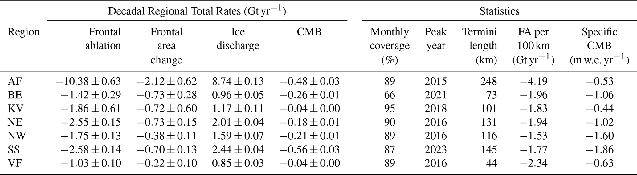
The three regions characterizing the island of Spitsbergen (NE, NW, SS) have comparable yet distinct rates, with all three regions peaking in 2016. The southern region loses the most mass to frontal ablation ($-\mathrm{2.58}\pm \mathrm{0.14}$ Gt yr⁻¹), closely followed by the northeast third ($-\mathrm{2.55}\pm \mathrm{0.15}$ Gt yr⁻¹), and lastly the northwest extent of the island ($-\mathrm{1.75}\pm \mathrm{0.13}$ Gt yr⁻¹). The final subregion, Vestfonna ice cap (VF), has the lowest decadal rate ($-\mathrm{1.03}\pm \mathrm{0.10}$ Gt yr⁻¹) of all regions. However, to facilitate comparisons among regions with different total calving front lengths, frontal ablation is also normalized by the total terminus length and expressed per 100 km of calving front (Table 2). VF has the second highest frontal ablation intensity rate (−2.34 Gt yr⁻¹ (100 km)⁻¹) of all regions, revealing the region's relevance for studying controls on and impacts of frontal ablation in Svalbard. Expectedly, AF exhibits the strongest frontal ablation intensity (−4.19 Gt yr⁻¹ (100 km)⁻¹), further demonstrating its dominant contribution to Svalbard's frontal ablation mass budget. Although the largest absolute CMB corrections occur in AF ($-\mathrm{0.48}\pm \mathrm{0.03}$ Gt yr⁻¹) and SS ($-\mathrm{0.56}\pm \mathrm{0.03}$ Gt yr⁻¹), the specific CMB (Table 2) is most negative in SS (−1.86 m w.e. yr⁻¹), NW (−1.60 m w.e. yr⁻¹), and BE (−1.06 m w.e. yr⁻¹), indicating that these regions experience the strongest climatic mass losses relative to their glacierized area. Regionally, the monthly measurement coverage is greater than 85 % for all subregions except BE (66 %), which is affected by a small sample size (714 possible months for 6 glaciers), as well as complex glacier geometries and outlet areas, leading to removed model prediction outliers.

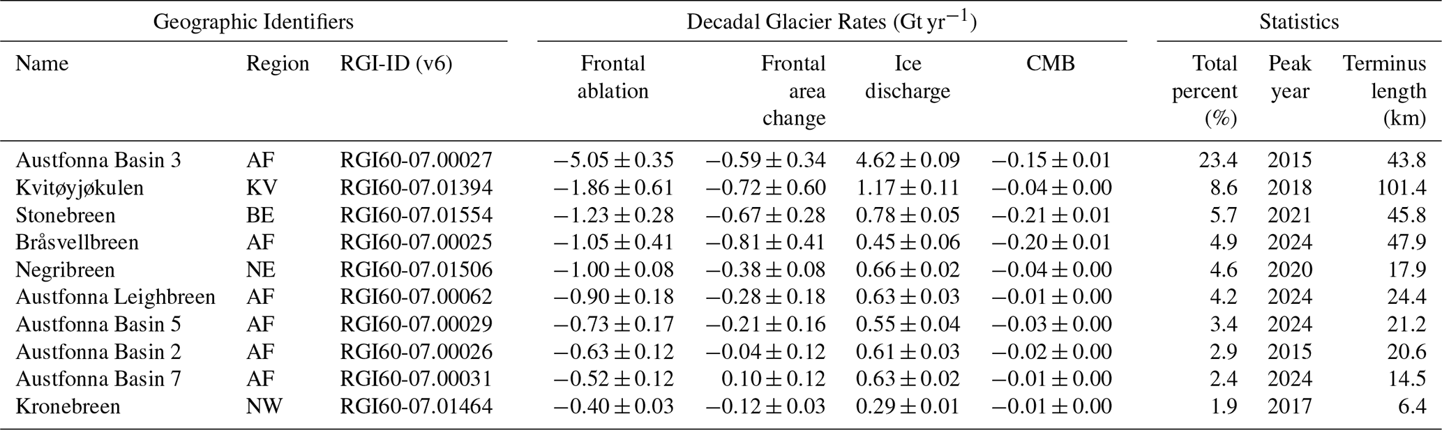
Table 3 Decadal frontal ablation, frontal area change, ice discharge, and CMB rates for the top 10 contributing glaciers to the total Svalbard frontal ablation rate. Glaciers are identified by their subregion and RGI-ID (version 6). Austfonna basins are defined in Dowdeswell et al. (2008) and Zheng (2022). Total percent is the glacier's contribution to the summed Svalbard decadal frontal ablation rate, peak year is the highest yearly rate of frontal ablation mass losses, and terminus length is the decadally-averaged ice front width.

4.3 Dominant glaciers

Across Svalbard, 47 % of the total decadal frontal ablation rate is explained by five key glaciers (Table 3), while 80 % is attributed to the top 27 contributors (Fig. 10), with the final 20 % accounted for by the remaining 120 glaciers. Overall, 20 glaciers contribute more than 1 % to the total decadal rate. Six of the top 10 glaciers are located on the Austfonna ice cap, however, the top five are distributed across four different regions (AF, BE, KV, NE). The previously described Austfonna Basin 3, Kvitøyjøkulen ice cap, and Stonebreen have the largest rates (38 % combined), with AF Basin 3 ($-\mathrm{5.05}\pm \mathrm{0.35}$ Gt yr⁻¹) contributing nearly 25 % to the Svalbard total. Kvitøyjøkulen's standing as the second highest contributor is attributable to its massive scale, with a staggering 101 km terminus subjected to calving, subaqueous and subaerial melt, and sublimation along the ice front.

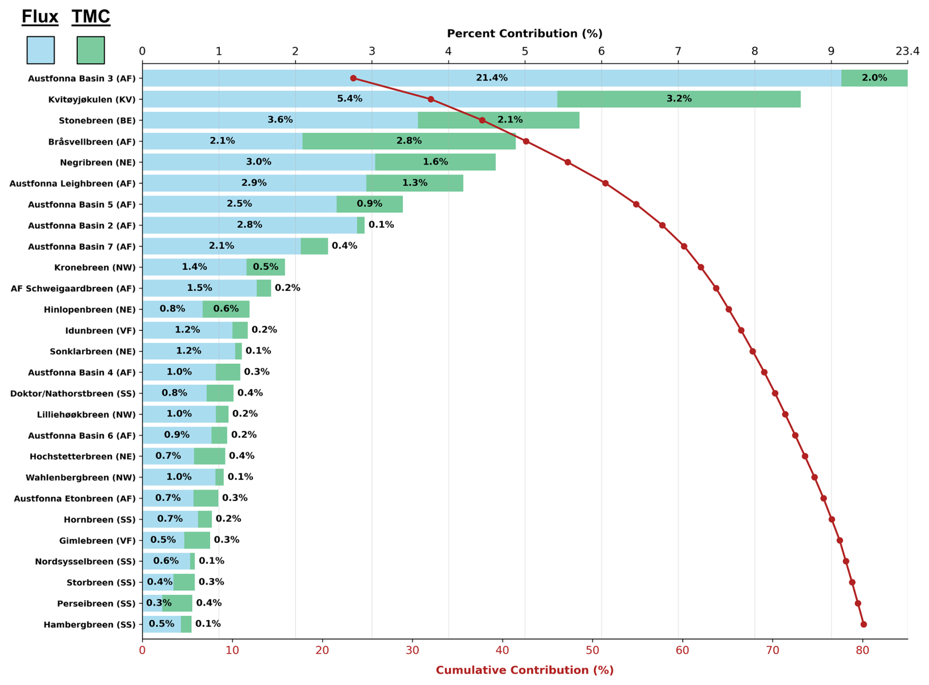
Figure 10 Percent contribution of individual, dominant glaciers to the total Svalbard frontal ablation rate, with 27 glaciers cumulating 80 % of the total (red line). The top 20 all account for at least 1 % of the total and are regionally distributed with nine in AF, four in NE, three in NW, and one in KV, BE, VF, SS. Component contributions of the ice discharge (flux) and terminus mass change (TMC) are partitioned for each glacier. The component percentages and their relative visual scaling for Austfonna Basin 3 are correct, however, due to its dominance in the Svalbard frontal ablation budget (23.4 %), the glacier was scaled to fit the figure (see top x axis).

The signal of frontal area change is greatest at Bråsvellbreen ($-\mathrm{0.81}\pm \mathrm{0.41}$ Gt yr⁻¹) due to a sustained retreat over the decade. Bråsvellbreen's location at the most southern extent of the AF ice cap might indicate an increased sensitivity to ocean temperature and dynamics, or its terminus changes might follow similar controls to the nearby AF Basin 3, which has a comparable area change magnitude ($-\mathrm{0.59}\pm \mathrm{0.34}$ Gt yr⁻¹). Influence of the CMB is most notable at Stonebreen, Bråsvellbreen, and AF Basin 3, stemming from the relatively upstream fluxgate placement, which exposes more ice surface area to climate effects. Interestingly, the fifth strongest frontal ablation contributor, Negribreen in NE ($-\mathrm{1.00}\pm \mathrm{0.08}$ Gt yr⁻¹), only has an ∼18 km terminus, compared to termini greater than 40 km for the other glaciers in the top five. Negribreen exhibited surge behavior and localized retreat patterns, accompanied by complex geometry changes at its ice front, explaining the large rate (Fig. 11). Normalized per 100 km of terminus, AF Basin 3, Negribreen, and the 10th strongest contributor, Kronebreen in NW, have the most intense frontal ablation intensity rates. While Kronebreen has the 10th highest rate, its decadal terminus length (6.4 km) ranks 30th; given its small size relative to other glaciers in the top 10, as well as its large frontal area change ($-\mathrm{0.12}\pm \mathrm{0.03}$ Gt yr⁻¹) and ice discharge (0.29±0.01 Gt yr⁻¹) rates, like Negribreen, Kronebreen is distinguished as a highly dynamic glacier. The four remaining glaciers in the top 10 are large basins of the AF ice cap, including AF Leighbreen and AF Basins 2-5-7. Though their frontal ablation rates range from −0.52 to −0.90 Gt yr⁻¹, the ice discharge is homogenous, with rates between 0.55 to 0.63 Gt yr⁻¹. The frontal ablation variability is due to frontal area change rates ranging from −0.28 to 0.10 Gt yr⁻¹. AF Basin 7 is the only glacier in the top 10 contributors to have advanced over the decade, with a positive frontal area change of 0.10±0.12 Gt yr⁻¹, though the uncertainty is greater than the frontal trend.

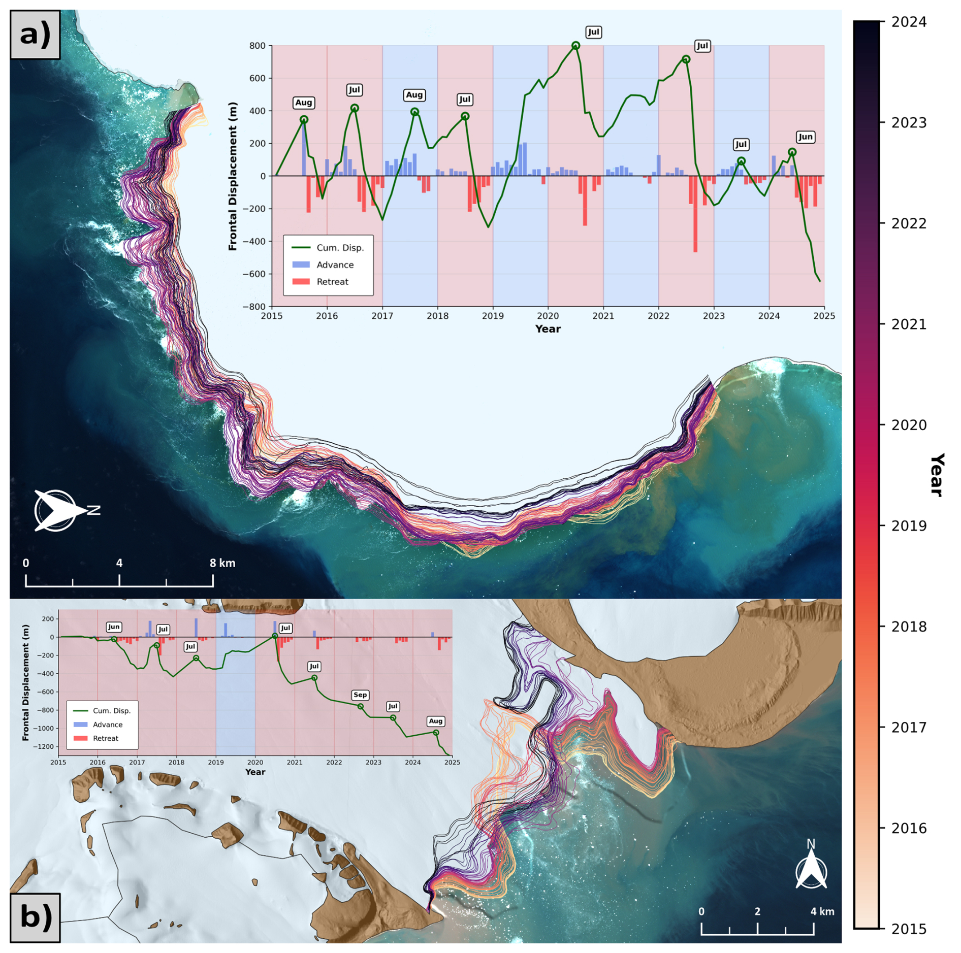
Figure 11 Frontal evolution of the destabilized Austfonna Basin 3 glacier and Negribreen, with monthly-averaged terminus predictions and a superimposed cumulative frontal displacement plot showing the monthly displacement signal for all available frontal positions. The monthly displacement bars are plotted to delineate retreating and advancing months, while each year is shaded light red or blue to indicate a retreat or advance between the first and last available terminus position in the given year. (a) Austfonna Basin 3 displays a seasonal cycle of advance until the annotated month, followed by a rapid retreat in all years except 2019 and 2021. The background is a Sentinel-2 image from 7 July 2022, and 112 of 120 monthly fronts are available. (b) Negribreen also has an annual retreat cycle in the second half of the year for all years except 2015 and 2019, however, with only 75 of 120 possible monthly front positions, the frontal trend in the first half of the year is mostly ambiguous. The background is a Sentinel-2 image obtained on 2 August 2019.

5 Discussion

5.1 Comparison to prior work

As this study is structured around the work established at Svalbard by Kochtitzky et al. (2022b), naturally our frontal ablation estimates may be compared due to a common definition of marine-terminating glaciers from their manually delineated termini in summer 2019. For consistency, we flip the signs of our frontal ablation rates, as equations were defined with contrasting sign in the studies. Kochtitzky et al. (2022b) computed separate frontal ablation estimates generalized to periods between 2000–2010 and 2010–2020; the computed temporal period varies glacier-to-glacier in Kochtitzky et al. (2022b) (i.e. not strict decades), however, all frontal ablation estimates are constrained within July 1999 through August 2011 in the 2000–2010 period and from July 2010 through August 2019 in the 2010–2020 period. Due to the variable temporal periods, like Kochtitzky et al. (2022b), we refer to these periods as 2000–2010 and 2010–2020. Nevertheless, a continuation of the long-term frontal ablation record in Svalbard is possible, given our study period's approximately five-year offset (January 2015 through December 2024) from the 2010–2020 period. Mass loss due to frontal ablation has rapidly increased since 2000, with regional rates reported in Kochtitzky et al. (2022b) of 7.62±2.65 and 16.82±2.48 Gt yr⁻¹ over their successive measurement periods (120 % increase), the former of which (2000–2010) is corroborated by another Svalbard-wide calving rate estimate (excluding KV) of 6.75±1.7 Gt yr⁻¹ between 2000–2006 (Błaszczyk et al., 2009). Though there is a five-year overlap with the 2010–2020 estimate, our annually averaged rate of 21.57±0.97 Gt yr⁻¹ reveals a sustained mass loss increase due to frontal ablation, and an 183 % increase in the rate from 2000–2010. All three long-term rates are outside the uncertainty range of each other, supporting the escalating trend in frontal ablation mass loss. In Kochtitzky et al. (2022b), the increasing frontal ablation rate is strongly driven by increased ice discharge with consecutive long-term rates of 4.88±1.98 and 14.41±1.05 Gt yr⁻¹, respectively. Conversely, terminus mass loss slightly decreased between their two periods, from −2.74 to −2.40 Gt yr⁻¹, contrasting with the shift in the relative importance of ice discharge and terminus mass loss in driving the increasing frontal ablation observed in our results. Although the long-term ice discharge trend is continuously increasing – with rates of 4.88±1.98, 14.41±1.05, and 17.75±0.20 Gt yr⁻¹ from 2000–2010, 2010–2020, and 2015–2024, respectively (∼25 % increase since 2010–2020) –, terminus mass loss (i.e. frontal area change – CMB) accelerated more rapidly from $-\mathrm{2.4}\pm \mathrm{2.25}$ Gt yr⁻¹ over 2010–2020 to $-\mathrm{3.82}\pm \mathrm{0.94}$ Gt yr⁻¹ over our study period (∼60 % increase). Indeed, the upper bound of the uncertainty range for the 2010–2020 rate reported by Kochtitzky et al. (2022b) overlaps with the lower bound of our long-term estimate, suggesting that the apparent increase in terminus mass loss should be interpreted with caution. Nevertheless, comparison of the two non-overlapping five-year periods within our record reveals substantially greater terminus mass loss during 2020–2024 than during 2015–2019, with mean rates of $-\mathrm{5.50}\pm \mathrm{1.27}$ and $-\mathrm{2.15}\pm \mathrm{1.40}$ Gt yr⁻¹, respectively. The 2015–2019 period includes two years of net terminus mass gain (2017 and 2019), which partially offset substantial mass loss in 2015, 2016, and 2018, whereas 2020–2024 was characterized predominantly by net mass loss, despite near-neutral change in 2021. Furthermore, because the 2010–2020 mean reported by Kochtitzky et al. (2022b) ($-\mathrm{2.40}\pm \mathrm{2.25}$ Gt yr⁻¹) is more negative than our 2015–2019 mean ($-\mathrm{2.15}\pm \mathrm{1.40}$ Gt yr⁻¹), terminus mass loss during 2010–2014 can be estimated at approximately −2.65 Gt yr⁻¹, assuming equal temporal weighting of the two five-year periods. Although the magnitude of terminus mass loss varied across these three consecutive five-year periods (2010–2014, 2015–2019, and 2020–2024), the substantial intensification during 2020–2024 provides an opportunity for future work to study the controls across Svalbard's tidewater glacier termini and build on the findings of recent studies (Foss et al., 2024; Holmes et al., 2019, 2023; Luckman et al., 2015; Nanni et al., 2025).

By volume, the long-term frontal ablation rate of 94 glaciers rose over the five-year offset between our study period and 2010–2020 in Kochtitzky et al. (2022b), compared to 53 with a reduced rate. However, by accounting for numerical noise of small glaciers with negligible frontal ablation, only 80 of 147 glaciers have an absolute long-term rate change greater than 0.01 Gt yr⁻¹, of which 60 and 20 glaciers increased and decreased, respectively. Overall, 16 glaciers had an absolute change rate exceeding 0.1 Gt yr⁻¹, with Austfonna Basin 3 the only glacier whose rate decreased in the subset from 6.10±0.24 Gt yr⁻¹ in 2010–2020 to 5.05±0.35 Gt yr⁻¹ in this study. Two case studies on Austfonna Basin 3 by Dunse et al. (2015) and Schellenberger et al. (2017) support our lower frontal ablation rate compared to Kochtitzky et al. (2022b); Dunse et al. (2015) estimated an iceberg calving rate of 4.2±1.6 Gt yr⁻¹ between 19 April 2012 and 9 May 2013, while Schellenberger et al. (2017) reported a 5.2±1.9 Gt yr⁻¹ frontal ablation rate from 19 April 2012 to 26 July 2016. Though AF Basin 3 is the overwhelming contributor to frontal ablation mass loss in Svalbard, results from both studies, combined with our more recent decadal rate, suggest that the rate of mass loss is stable since the destabilization in 2012. Besides AF Basin 3, the other four glaciers with positive long-term rate changes exceeding 0.5 Gt yr⁻¹ between this study and Kochtitzky et al. (2022b) are all top five frontal ablation contributors in Svalbard (see Sect. 4.3), with the following magnitude increases in Gt yr⁻¹: Negribreen (0.78), Kvitøyjøkulen (0.57), Bråsvellbreen (0.53) and Stonebreen (0.51). The acceleration of Negribreen is especially noteworthy, increasing its frontal ablation rate by ∼375 % from 0.21±0.15 Gt yr⁻¹ in 2010–2020 to 1.00±0.08 Gt yr⁻¹ over 2015–2024. Consequently, we recommend Negribreen as a prime case study candidate to understand frontal ablation controls and build upon the recent investigation of surge mechanisms driving the glacier's frontal destabilization and geometric change (Haga et al., 2020; Middleton et al., 2025). In addition, we assessed whether differences in ice thickness reconstruction methods could contribute to the glacier-scale differences in frontal ablation estimates. This study derives ice thicknesses (Sect. 3.2.2) from the SVIFT thickness dataset (Fürst et al., 2018a), whereas Kochtitzky et al. (2022b) primarily used spatially distributed GlaThiDa observations supplemented by Millan et al. (2022) modeled thickness estimates where observations were unavailable. Comparison of mean ice thicknesses at the fluxgates shows a mean absolute difference of 37.7 m (RMSE = 47.3 m) across the 147 glaciers (see supplement Fig. S5). However, absolute thickness differences are not significantly correlated with absolute frontal ablation differences (Pearson $r=-\mathrm{0.08}$, p=0.31), suggesting that differences between the thickness datasets are unlikely to be the dominant explanation for the glacier-scale differences in frontal ablation estimates.

Like Li et al. (2025), we detect widespread retreat across Svalbard's tidewater glaciers, with 119 glaciers having a negative width-averaged frontal displacement between their first and last ice front position in the time series, while 28 exhibit calving front advance indicated by positive displacement. Nuancing the terminus position trends for scale, only nine advancing glaciers (eight of which surged; Strozzi et al., 2026) have an area gain exceeding 1 km² – Borebreen and Sefströmbreen in NW, Austfonna Basin 2 and 7 in AF, and Strongbreen, Kvalbreen, Recherchebreen, Arnesenbreen, Skobreen (Paulabreen) in SS – opposed to 59 with a retreat area greater than 1 km². We cannot directly compare terminus trends with Li et al. (2024) due to differences in tidewater glacier selection and partitioning of ice streams into singular or distinct terminus features. However, our studies share 130 commonly defined glaciers, of which 120 may be compared, as Li et al. (2024) defined 10 surge-type glaciers without providing a retreat or advance classification. We have an 83 % agreement rate across 100 glaciers, with differing calving front trends for the remaining 20 glaciers, owing to recent calving front changes monitored in this study. Of the divergent subset, seven are explained by frontal advance in 2023 and 2024, which is just beyond or on the fringe of the 1985–2023 study period in Li et al. (2024). Similarly, four more glaciers began rapid retreat phases in 2024, resulting in terminus shifts behind the reference state in 2015, and consequently, contrasting movement regimes. Another eight disagreements are attributable to glaciers with stagnant fronts and negligible terminus position variability, where the decadal area change and frontal displacement is less than 0.2 km² and 100 m, respectively. Particularly noteworthy, the final disagreed glacier is the dominant Austfonna Basin 3, which, apart from a stable advance in 2019 and to a lesser degree in 2021, has a consistent seasonal cycle of frontal advance in the first half of the year (Fig. 11), followed by rapid retreat in the second half from 2015–2024, also reported by Li et al. (2024) from 2014–2023. The decadal area difference between February 2015 and December 2024 reveals a retreat of ∼30 km² and a negative width-averaged frontal displacement of ∼800 m, averaged over a ∼37.5 km terminus length in December 2024.

6 Code and data availability

The monthly frontal ablation, ice discharge/velocity, and calving front datasets, as well as relevant vector geometries (regional zone labels, fluxgates/points, RGI boxes, etc.), are publicly available in version 4 of the dataset at https://doi.org/10.5281/zenodo.19481461 (Pyles et al., 2026). Jupyter notebooks with the code developed for this study – processing geometries, training data, image preprocessing, model prediction and outlier postprocessing, frontal uncertainty evaluation, ITS_LIVE velocity, ice discharge computation, and frontal ablation computation – are provided as well.

The code for the multi-temporal segmentation model is publicly available in Dreier et al. (2026b). The CaFFe benchmark dataset, which the model is pretrained on, is publicly available at https://doi.org/10.1594/PANGAEA.940950 (Gourmelon et al., 2022b).

7 Conclusions

We conclude by reflecting on the methodological framework developed in this study and outlining recommendations for future studies to improve the process understanding of frontal ablation. To begin, while linear interpolation across temporal gaps bounded by frontal geometry is a reasonable assumption, future studies mapping calving fronts with a segmentation model for subsequent glaciological applications may benefit by providing complete frontal information at the target resolution. Building on the foundation of SAR image segmentation in this study, missing frontal geometry could be addressed with two complementary approaches, which were not implemented here as the suggestions are reflections on the methodology after the large-scale bulk data processing and frontal ablation application: (1) besides the Kvitøyjøkulen ice cap which lacked IW mode Sentinel-1 SAR data, this study did not leverage the available Sentinel-1 record of EW mode acquisitions, which indeed have a coarser 40 m resolution compared to the 10 m IW mode, yet, EW scenes have proven to be functional for segmentation applications and are an untapped resource; (2) missing monthly terminus positions may be linearly interpolated between the ice-ocean boundaries of the first and last available monthly-averaged segmentation predictions bounding the gap. Such a workflow could enable a total summation of the frontal ablation at the annual and decadal levels.

We suggest future frontal ablation studies focus on the controls and forcings (oceanic, climatic, dynamical, fjord and glacier geometry, ice mélange and buttressing, bathymetry, etc.) of frontal ablation at glacier and sub-regional scales, build stronger links between the timing of terminus displacement and frontal ablation response, and discern how subglacial hydrology systems and submarine melt variability impact frontal ablation magnitude and observed terminus geometry changes. This study provides an ideal database (https://doi.org/10.5281/zenodo.19481461; Pyles et al., 2026) for such further analysis and for addressing persisting knowledge gaps by providing unprecedented spatially and temporally detailed information on frontal ablation and its components throughout Svalbard. Furthermore, the modeling community can harness the high spatio-temporal resolution of the dataset to calibrate models, tune parameterizations, and improve the deficient representation of frontal ablation in model outputs.