Marine Heat Waves and Cold Spells – Multiple Analysis/Definitions (MHW-MAD): A Multi-Definition Global Marine Heatwave Database from Satellite Sea Surface Temperature Data

Marine heatwaves (MHWs) are prolonged anomalies of warm sea surface temperature (SST) that can disrupt marine ecosystems, physical climate processes, and human coastal activities. MHW definitions vary due to different stakeholders requirements, such as ecological scientists and climate scientists having differing yet specific thresholds and metrics. Here we introduce a new global database of daily MHW metrics: climatological baselines, threshold exceedances, SST anomalies, and categorical event classifications of severity, derived from the European Space Agency SST Climate Change Initiative (ESA SST CCI) climate data record (CDR; 1982–2021) version 3.0 and an extension from 2022–2024 provided as an interim climate data record (iCDR). Building on the widely used definition of MHWs, periods in which SST exceeds the local 90th percentile for 5 or more days, our database extends this framework by incorporating multiple baseline climatologies (including fixed 30-year periods and rolling 30-year windows, as well as the period for reanalysis 1993–2022), varied percentile thresholds (90th, 95th, 99th), and both raw and linearly detrended SST anomalies. We also implement alternative event duration criteria (minimum 10 and 30 d persistence) to classify longer-lasting warm events. In addition to warm extremes, we provide marine cold spell (MCS) indices derived from the 1st, 5th and 10th percentiles, enabling analysis of cold as well as warm ocean extremes within the same framework. All data products are provided at daily resolution on a 0.05° (∼ 5 km) grid, with outputs including daily climatological percentiles, SST anomalies and binary MHW flags with severity category indices. This comprehensive database provides a consistent foundation for detecting and analysing MHWs across time and space, enabling researchers to assess how methodological choices affect MHW characterisation. By offering multiple definitions in parallel, the database facilitates intercomparison studies and supports applications from climate monitoring and model evaluation to marine ecological impact assessment, thereby providing users with pre-made indices for extremes, with the ambition to be rolled out into the future with new data releases. The dataset is available at https://doi.org/10.5281/zenodo.21835325 (Hayward et al., 2026).

1 Introduction

Marine heatwaves (MHWs) are discrete, prolonged periods of abnormally high ocean temperatures relative to typical local conditions (Hobday et al., 2016). They often persist for days to months and can extend over vast regions (> 1000 km²). MHWs can have important ecological and socioeconomic impacts. For example, extreme warming events have caused mass mortalities of marine organisms and biodiversity loss, including coral bleaching events (Garrabou et al., 2019), harmful algal blooms (Roberts et al., 2019), shifts in species distributions (Lonhart et al., 2019), and declines in fisheries (Wernberg et al., 2016; Smale et al., 2019; Gonzalez et al., 2025). Demonstrating these effects, an intense MHW off Western Australia in 2011 removed ∼ 100 km of kelp forests (∼ 90 % of the region's kelp), leading to a regime shift in the local ecosystem (Wernberg et al., 2016). Such events threaten the resilience of marine ecosystems and the services they provide to coastal communities.

There is clear evidence that the frequency and intensity of MHWs are increasing under climate change (Frölicher et al., 2018; Lien et al., 2024). Long-term analyses indicate that from 1925 to 2016, the average annual number of MHW days has increased globally by over 50 % (Oliver et al., 2018). In recent decades, many MHWs have been attributed to anthropogenic warming (Oliver et al., 2018; Smale et al., 2019), and are expected to increase in frequency by the end of the century (Frölicher et al., 2018). In particular, the duration and spatial extent of MHWs have expanded, coincident with the rise in baseline ocean temperatures. These trends underscore the urgency of monitoring MHWs as well as understanding their drivers.

Despite growing research, there is still ongoing debate on how best to define and detect MHWs across different studies (Farchadi et al., 2025; Smith et al., 2025), with the most common definition taken from Hobday et al. (2016). How MHWs are identified depends on methodological choices including the baseline climatology period, threshold percentiles, and minimum duration, among other factors. Some studies use a fixed historical baseline (e.g. 30-year climatology) whereas others use a shifting baseline that moves with each year. In a warming climate, a fixed baseline (such as the standard World Meteorological standard 30-year baseline between 1991 to 2020) will likely label more recent warm events as extreme (Oliver et al., 2018) compared to a moving baseline (or periodically updated “normal”). A shifting baseline effectively raises the threshold over time, filtering out the warming (or cooling) trend and highlighting interannual variability. Similarly, choosing a 90th percentile threshold versus a more extreme 95th or 99th percentile can substantially change which events qualify as MHW. The required duration matters as well too; the original Hobday et al. (2016) definition requires ≥ 5 consecutive days, but some applications consider longer minima (e.g. 10 d or more) to isolate only the most persistent events. Due to the vast array of methodological differences, recent studies have called for clearer and more standardised MHW definitions to aid comparisons and decision-making (Amaya et al., 2023; Farchadi et al., 2025).

To address these differences, we present a “multi-definition” global MHW database that allows users to examine events under a suite of definitions within a single, consistent framework. We derive this database from the European Space Agency SST Climate Change Initiative (ESA SST CCI) Climate Data Record (CDR) v3.0 (Embury et al., 2024), which combines data from different satellite sensors into a daily 0.05° gridded gap-free SST product (in the future we plan to incorporate more SST products).

The MHW database provides multiple climatological baselines (both a fixed 30-year baseline and rolling 30-year windows) so that users can explore the influence of baseline period on detected MHWs. We include both raw and detrended SST anomaly fields, enabling analysis of MHWs with and without the long-term warming signal. Furthermore, we provide event detections based on the standard 90th-percentile/5 d definition, but also on more stringent threshold exceedances (95th and 99th percentiles) and longer minimum durations (10 and 30 d). By offering these options side-by-side, the database facilitates comparative studies of how MHW properties change under different definition choices. In the following, we describe the data sources and processing methods, present example results comparing definitions including a case study of the 2014 “Blob” event in the Northeast Pacific (Bond et al., 2015), an unusually large and persistent MHW (2013–2016) that disrupted ecosystem processes, causing mass mortalities (Renner et al., 2024). Further to this, we detail data availability and potential uses, and examine the broader implications of this multi-definition approach.

2 Sea Surface Temperature Data

The ESA SST CCI CDR v3.0 CDR and ICDR are based on the same software and systems, which ensures a consistent and uninterrupted daily global SST time series covering the years 1982 through 2025. In this study, the Level 4 (L4) analysis product is used, which combines SST observations from multiple satellite instruments into a daily gridded gap-free product at 0.05° × 0.05° resolution. The L4 analysis product integrates infrared and microwave sensor SST retrievals from 22 different satellite missions (Embury et al., 2024). The infrared and microwave signals were collected from the following four series of sensors: 15 Advanced Very High Resolution Radiometers (AVHRRs), three Advanced Along-Track Scanning Radiometers ((A)ATSR), two Sea and Land Surface Temperature Radiometer (SLSTR) and two Advanced Microwave Scanning Radiometers (AMSRs). The L4 analysis product is produced using the climate configuration of the Operational Sea Surface Temperature and Ice Analysis (OSTIA) system (Donlon et al., 2012; Good et al., 2020), which blends the input SST data from multiple satellite sensors and corrects for diurnal warming and depth-based temperature gradients, by standardising SST values to ∼ 20 cm depth. Unlike the OSTIA reprocessed L4 database (Good et al., 2020), the ESA SST CCI system does not assimilate in situ data into its L4 product, thereby preserving satellite-derived trends.

The ESA SST CCI CDR v3.0, is specifically designed for robust climate research through rigorous inter-sensor calibration and bias corrections (Embury et al., 2024). As a result, the physics-based retrieval algorithms generate a stable, low-bias SST database that is largely independent of in situ observations. The CCI SST L4 SST product adheres to Group for High Resolution SST (GHRSST) standards, delivering daily, gap-free global SST fields ideal for the assessment of MHWs (Yang et al., 2021). Furthermore, the SST CCI v3.0 has been proven as a suitable product for long-term ocean climate studies, including the detection and characterisation of MHWs (Yang et al., 2021). This being said, the approach taken can be implemented on different SST products and algorithms, and we hope to explore this in the future.

3 Marine Heatwave Definitions and Framework

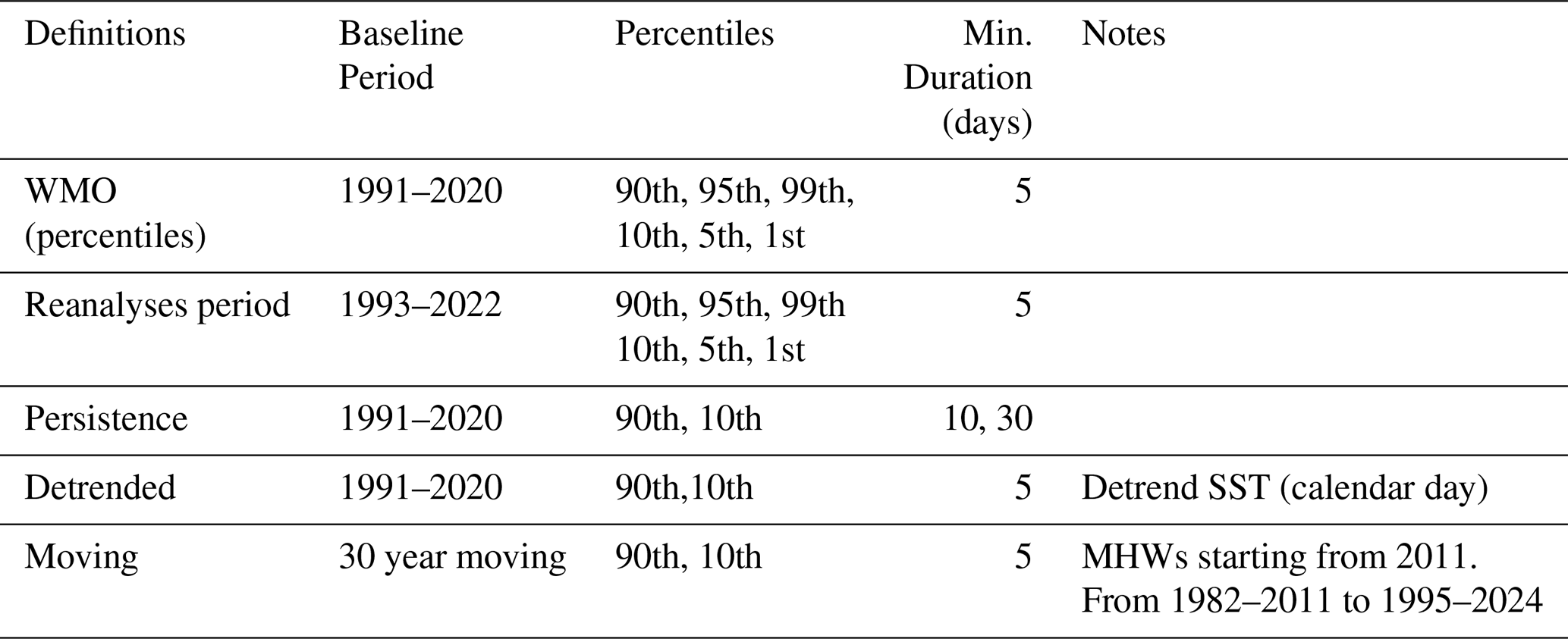
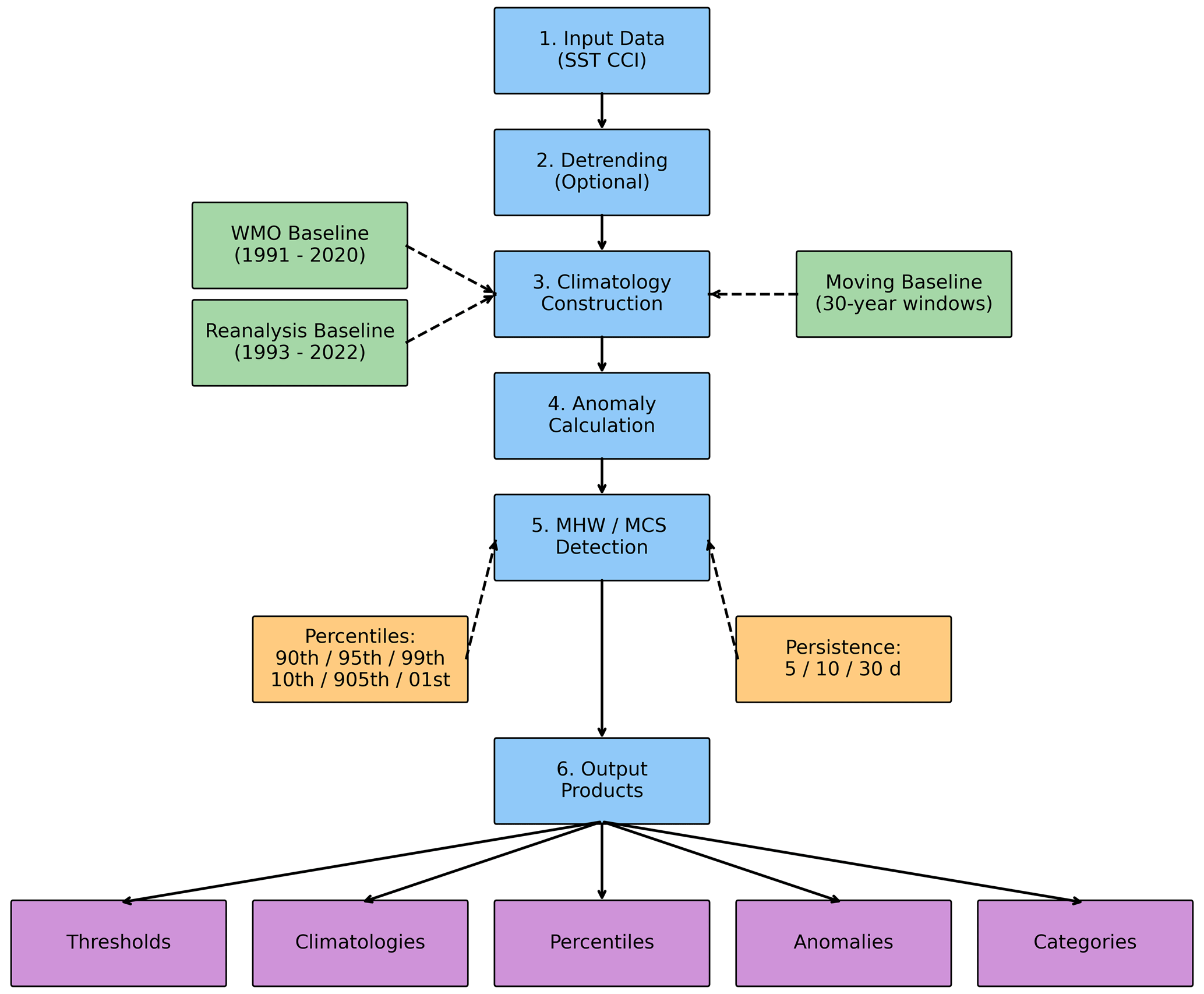
Definitions of MHWs were selected and assessed, based on percentiles, baselines, persistence, and detrended data. All data processing was performed using Python and Climate Data Operators (CDO) software 2.1.1, with some of the post-processing also done with the help of NCO 5.2.1. We first computed long-term climatologies for each grid cell and day-of-year (DOY) using multiple baseline definitions (Fig. 1). We then calculated daily SST anomalies relative to those climatologies and identified MHW by applying threshold criteria to the anomaly time series, as in Hobday et al. (2016). We then categorised the intensity of detected events using the severity index of Hobday et al. (2018) and organised all output variables into CF compliant NetCDF files, for 10 different sets of definitions (Fig. 1; Table 1). The same framework is applied symmetrically to the lower tail of the distribution to provide marine cold spell (MCS) indicies (Sect. 3.6). All the framework steps are described in detail in the following paragraphs.

Table 1 Definitions used to build the MHW-MAD database.

Figure 1 Workflow for creating daily MHW metrics based on different definitions.

3.1 Detrending of SST Time Series

Long-term ocean warming elevates the baseline SST over time for most areas, causing more frequent MHWs in later years if the baseline remains static. To allow users to separate the effect of global warming from natural variability, we created a detrended version of the SST record. In areas without strong decadal variability, removing the trend ensures that the baseline climatology represents the stationary seasonal cycle, so that anomalies and MHW detections reflect short-term fluctuations rather than the slowly shifting mean (Schlegel et al., 2019). This approach can be useful for attribution studies, as MHW occurrence after detrending can be interpreted as the portion driven by natural variability without the influence of long-term climate warming.

We applied a grid-point-specific linear detrending to the SST time series for each calendar day-of-year. For each grid cell, all SST values corresponding to the same calendar date across 1982–2024 were collated (e.g., all 15 January values over the 44-year span). We then performed an ordinary least squares linear regression of SST against the year for each calendar date at each grid cell. This yields a linear warming (or cooling) rate for that date and location (Fig. 2). The linear trend component for a given day was then subtracted from the original SST value. Detrending was applied at all grid cells regardless of statistical significance to ensure the database remained gap-free. The result is a parallel SST database where each grid cell's time series has no linear trend over 1982–2024. It is important to note that the detrending was only undertaken for the standard Hobday MHW definition of exceedance of the 90th percentile, 5 d persistence, and WMO climatology (1991–2020).

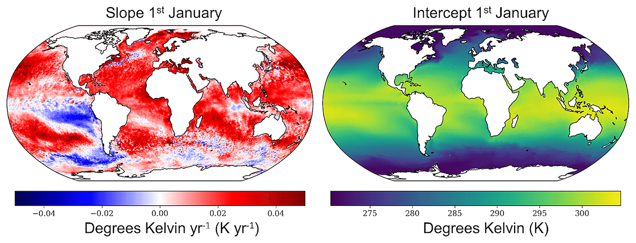
Figure 2 The slope and intercept used for detrending SST CCI data. The example shown is for 1 January.

3.2 Climatology Construction

We defined the climatological baseline as the distribution of SST for each DOY at each grid point, against which anomalies and extremes are measured. Two approaches were used to construct climatologies:

• a.

  Fixed 30-year climatology and reanalysis: We adopted the 30-year period 1991–2020 as a representative modern baseline, consistent with WMO-recommended climate normal periods (WMO, 2023) – and hereby refer to this as the “WMO baseline” (Fig. 3). For day (DOY 1–366) in all baseline periods, we aggregated all SST values for that same DOY, including 29 February across the 30 years. This yielded, for each grid cell and each DOY, a distribution of values. From this distribution, we computed the mean climatology together with the 1st, 5th, 10th, 50th, 90th, 95th and 99th percentiles of SST. The lower percentiles (1st, 5th and 10th) provide the thresholds required for marine cold spell detection while the upper percentiles (90th, 95th and 99th) provide MHW thresholds. To remain consistent with the methodology of Hobday et al. (2016), we adopted their two-stage smoothing. First, the seasonal climatology and percentile thresholds for each DOY were estimated from an 11 d window (±5 d) centred on that DOY, pooling all values within that window across every year of the baseline period. Second, a 31 d moving average (wrapped from 31 December to 1 January, when required) was applied to the resulting climatology and threshold time series. This two-step smoothing reduces sampling noise and prevents abrupt day-to-day jumps in the thresholds, while limiting the influence of individual extreme years on the percentile estimates.

• b.

  Moving 30-year climatology: As the ocean's climate is non-stationary, and warming has been prevalent over the past decades, we computed a series of moving-window climatologies. Starting with the earliest period of 1982–2011, we then advanced the 30-year window by one year at a time (i.e. 1983–2012, 1984–2013… up to 1995–2024). For each window, we calculated daily percentiles using the same method detailed above. The result is a time-evolving climatology that gradually warms (or cools) in most areas over time (Fig. 4). As a consequence of a shifting baseline, extreme anomalies are measured relative to the local contemporary climate for each year, rather than a historical reference period.

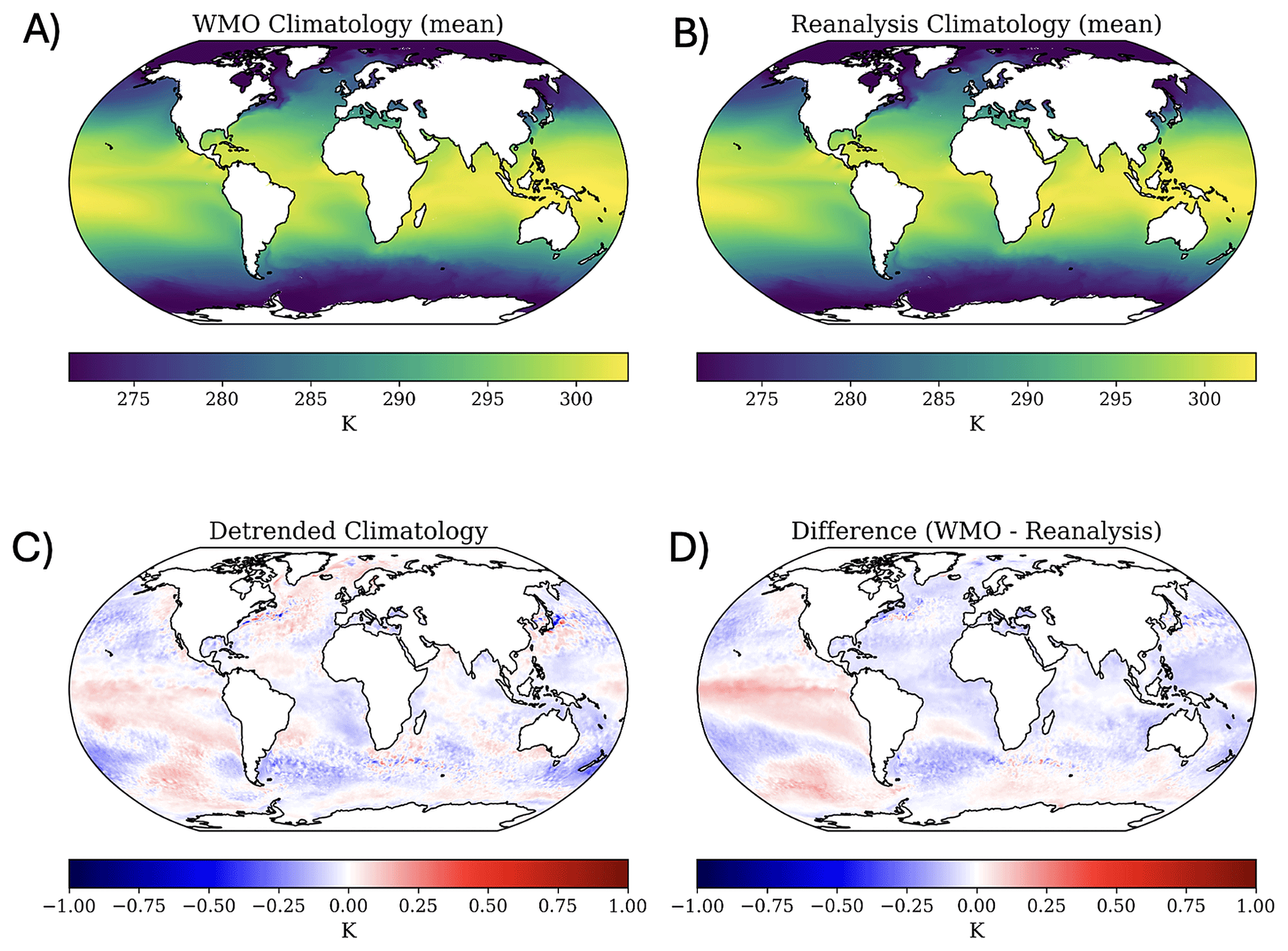
Figure 3 Different climatologies, including: (A) WMO climatology (1991–2020), (B) Climatology based on the reanalysis period (1993–2022), (C) Climatology based on detrended data for the WMO period, and (D) Difference between the WMO climatology and the climatology based on the reanalysis period.

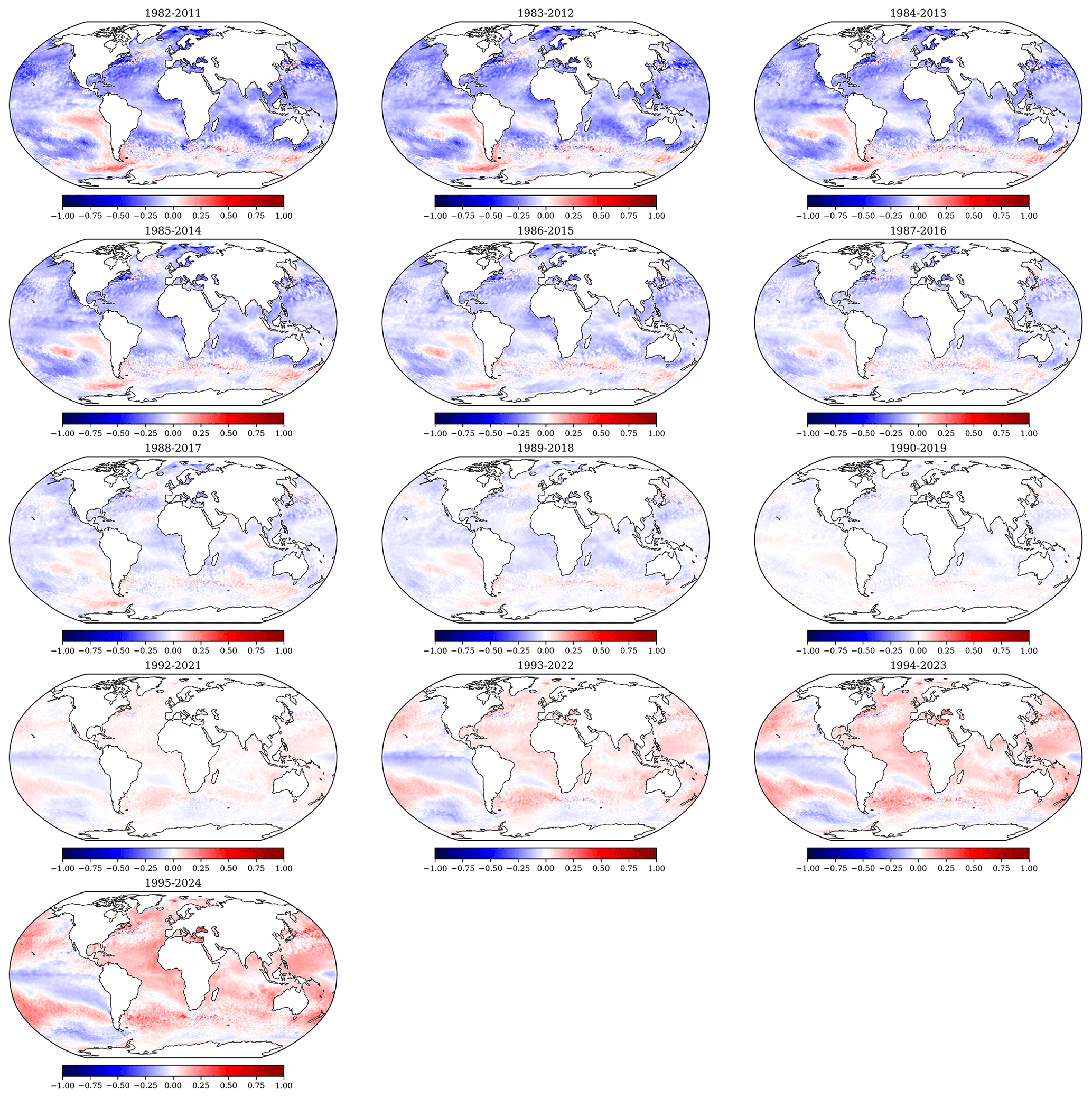
Figure 4 30-year moving climatologies from 1982–2011 to 1995–2024, based on the WMO definition. Each panel shows the difference to the WMO 1991–2020 climatology for 1 January for each respective period.

3.3 Anomaly Calculation

For each day in the record, we calculated SST anomalies as the deviation from the climatology on that DOY. Let SST_x denote the daily sea surface temperature (SST) at a given DOY (x), and M_x the mean climatology for that DOY. The anomaly is then defined as: anomaly = SST_x − M_x. In the anomaly calculations, we used a 366 d climatological reference that explicitly includes 29 February (DOY 60). Following Hobday et al. (2016), for non-leap years the climatology and threshold values for DOY 60 were obtained by linear interpolation between the values for DOY 59 (28 February) and DOY 61 (1 March) prior to computing anomalies and detecting events. This interpolation preserves a continuous one-to-one correspondence between calendar days and the 366 d climatological reference, ensuring that anomalies in non-leap years are correctly aligned with those from leap years, while avoiding artificial discontinuities around late February and early March. Anomalies were calculated independently using the fixed-baseline, moving-baseline, and also for the raw and detrended SST data records. These daily anomaly fields form the basis for MHW detection. Positive anomalies indicate warmer-than-normal conditions; negative anomalies indicate colder-than-normal conditions (i.e. used to detect cold spells).

3.4 MHW Detection

MHWs were identified by applying the threshold criteria to the SST anomalies. Following the framework of Hobday et al. (2016), an MHW is detected at a given grid cell whenever the SST (anomaly) exceeds a threshold (90th, 95th or 99th) for a minimum duration of 5 d (or more). This yields a binary MHW mask indicating the presence/absence of an MHW at each grid cell each day. We implemented multiple threshold and duration combinations:

• Extended thresholds: In addition to the 90th percentile from Hobday's definition, we also used 95th and 99th percentile thresholds (Fig. 5). These higher thresholds capture the more extreme temperature anomalies. Using the 95th or 99th percentile substantially reduces the number of events detected, focusing on the upper tail of extreme warm events. By comparing results from 90th vs. 95th vs. 99th percentile criteria, users can gauge the sensitivity of MHW statistics to the extremeness of the threshold.

• Extended persistence criteria: We also include longer minimum durations for MHWs. We required events to last at least 10 consecutive days above the threshold (instead of 5). We also created another more extreme criteria, where 30 d of consecutive exceedance were required. Naturally, imposing a longer duration criterion filters out shorter temperature anomalies. The 30 d criterion is more restrictive and captures only the most prolonged marine heatwave episodes. These longer-duration definitions can be useful for focusing on events likely to have consequential physical or ecological impacts.

• Event metrics: We have provided the day-by-day anomaly values and threshold exceedance status (Fig. 5), along with severity category (see Sect. 3.5), so users can examine the temporal evolution of each event. Here, we do not assign spatial extents or track contiguous areas of MHW, though such analyses could be done using this database.

• Ice-covered regions: In areas of sea ice cover, the SST-CCI product provides a value corresponding to the assumed freezing point of sea water of about −1.8 °C (assuming salinities of ∼ 33 PSU). As a result, areas of multi-year sea ice cover have threshold values of 0 (Fig. 5). As both the Arctic and Antarctic have witnessed pronounced sea ice loss in recent times (Stroeve et al., 2007; Purich and Doddridge., 2023), new areas of open water would be classified as marine heat wave hot spots due to their low thresholds, making ecological assessments of SST in polar regions challenging (Hayward et al., 2025; Pecuchet et al., 2025). To study polar regions, we suggest using targeted products such as the dedicated Arctic product produced in Copernicus Marine Service (CMEMS), L4 Arctic Ocean – Sea and Ice Surface Temperature Analysis (SST/IST; Nielsen-Englyst et al., 2024) or for Antarctic applications the C3S global L4 SST/IST product produced by the Danish Meteorological Institute (DMI), which in both cases provide satellite-observed sea-ice surface temperatures in sea ice covered areas, and blends the SST and IST observations in the marginal ice zones. MHW analyses based on these products have not been included here.

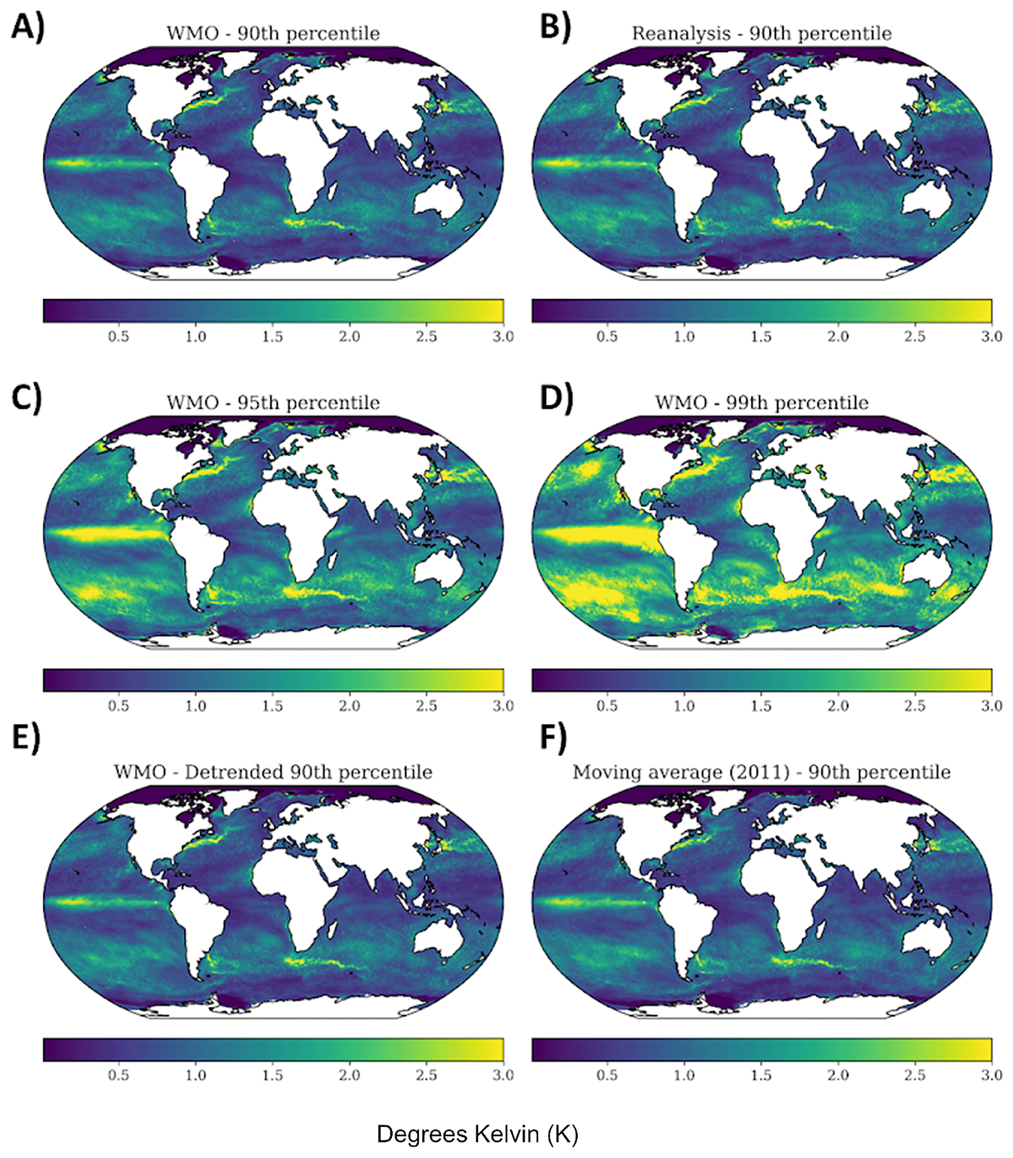
Figure 5 Marine heat wave anomaly threshold values (DOY = 1) based on different criteria using for 1 January. (A) the WMO climatology and 90th percentile threshold, (B) the reanalysis period (1993–2022) and a 90th percentile threshold, (C) the WMO climatology with the 95th percentile threshold, (D) the WMO climatology with the 99th percentile threshold, (E) the detrended data with a 90th percentile threshold, and (F) the moving average centred at 2011, with the 90th percentile threshold.

3.5 Categorical Severity Index

In addition to the binary identification of MHW days, we also provide a categorical severity index following the approach of Hobday et al. (2018) for classifying MHW intensity levels. Specifically, we define four categories of MHW intensity at each grid cell and day by comparing the SST anomaly to the local threshold difference.

1. Category 1 (“moderate”) corresponds to anomalies just above the threshold (anomaly ≥ threshold and < 2 times threshold difference),

2. Category 2 (“strong”) for anomalies 2–3 times the threshold difference,

3. Category 3 (“severe”) for 3–4 times, and

4. Category 4 (“extreme”) for anomalies ≥ 4 times the threshold difference.

These provide a simplified way to communicate the severity of an ongoing MHW. We compute such categories for each threshold definition (e.g., 90th, 95th, or 99th percentile) as separate files; a category 4 event for the 99th percentile threshold would only capture very extreme events, indicating using severity indices could also be a good way to track more extreme events instead of higher percentile thresholds. In the database, days with no MHW are given a category value of 0.

3.6 Marine Cold Spells

We additionally provide marine cold spell MCS indices, computed symmetrically to MHWs. MCSs are detected where the daily SST anomaly falls below the lower percentile thresholds (10th, 5th or 1st percentile) of the local climatology for a minimum of five consecutive days, following the cold-spell analogue of Hobday et al. (2016, 2018) and Schlegel et al. (2019). As for MHWs, we provide a categorical severity index, where Category 1 (“moderate”) corresponds to anomalies just below the 10th-percentile threshold (between one and two times the threshold difference), and Categories 2–4 (“strong”, “severe” and “extreme”) correspond to anomalies between two-to-three, three-to-four, and more than four times the threshold difference, respectively. MCS thresholds, anomalies and categories are provided alongside the MHW products for the WMO (1991–2020) baseline, enabling consistent analysis of both warm and cold ocean extremes within a single framework (Fig. 6).

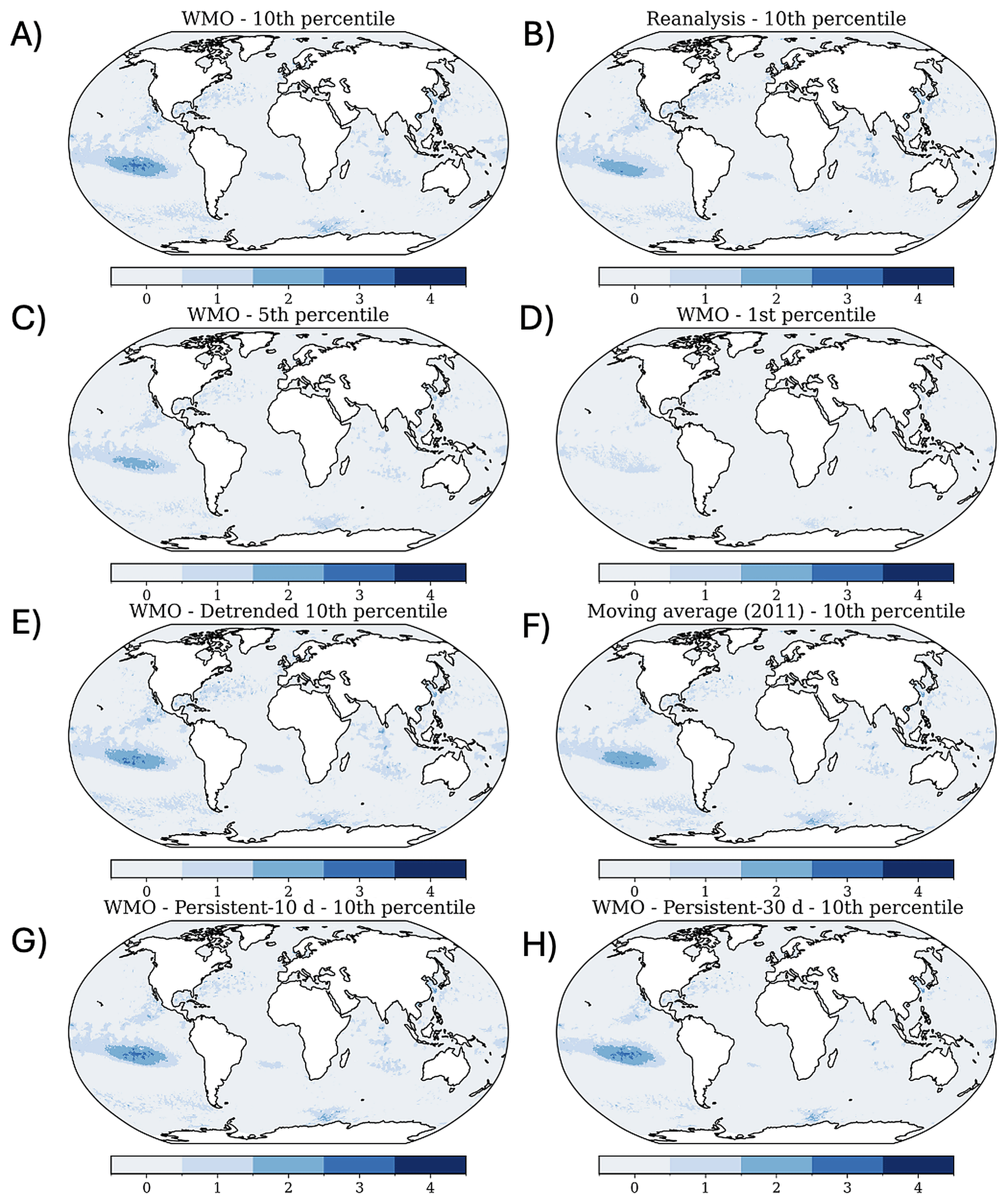
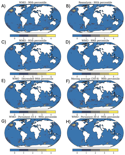
Figure 6 Categories of marine cold spells (MCS) on 1 January 2011 using different definitions, shown as the cold-spell analogue, Where (A) uses the WMO climatology (1991 to 2020) and the 90th percentile, (B) uses the reanalysis period (1993–2022) and the 90th percentile, (C) uses the WMO climatology and the 95th percentile, (D) uses the WMO climatology and the 99th percentile, (E) uses the WMO climatology and the 90th percentile with detrended data, (F) uses a climatological period between 1985 and 2014, and the 90th percentile, (G) uses the WMO climatology and the 90th percentile with a 10 d persistence window, and (H) uses the WMO climatology and the 90th percentile with a 30 d persistence window.

4 Results

Below we briefly discuss the effect of each MHW definition based on data from the 1 January 2014, during the event of the Pacific Blob (Fig. 7), we however note that our descriptions are only from a single day, and may not represent longer term trends.

4.1 Baselines/climatologies

Baseline effect – Using the fixed WMO baseline yields lower percentile thresholds than a climatology using later years (e.g. 1995–2024). As such, recent anomalies are more frequently flagged as MHWs,  and with higher severity than when using warmer climatological periods from later years, as evidenced from the Pacific Blob (Fig. 7).

Detrended effect – Removing each grid-cell's linear trend before building the climatology reduces the warming signal embedded in the thresholds, as also discussed in Schlegel et al. (2019). Globally, the share of MHWs was reduced when detrended SST is used, compared to its non-detrended counterpart (Fig. 7), however, the effect was very minor for the Pacific Blob (Fig. 7), indicating that the event was not attributed to long-term warming.

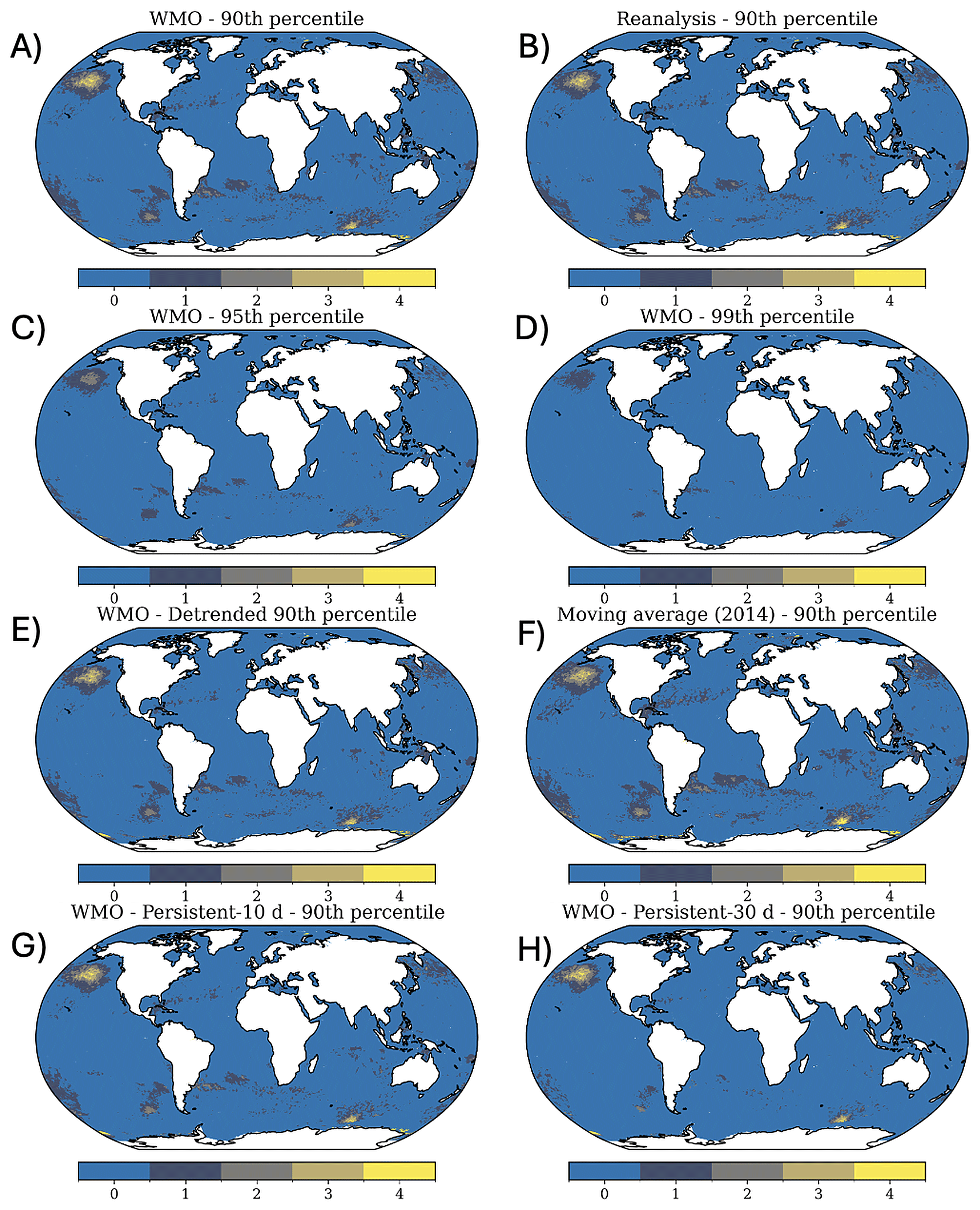
Figure 7 Categories of marine heat waves on 1 January 2014 (during “the Blob” event) using different definitions. Where (A) uses the WMO climatology (1991 to 2020) and the 90th percentile, (B) uses the reanalysis period (1993–2022) and the 90th percentile, (C) uses the WMO climatology and the 95th percentile, (D) uses the WMO climatology and the 99th percentile, (E) uses the WMO climatology and the 90th percentile with detrended data, (F) uses a climatological period between 1985 and 2014, and the 90th percentile, (G) uses the WMO climatology and the 90th percentile with a 10 d persistence window, and (H) uses the WMO climatology and the 90th percentile with a 30 d persistence window.

4.2 Sensitivity to Threshold, Persistence and Detrending

Raising the percentile threshold or minimum duration acts as an increasingly strict filter on detections (Fig. 7). Generalised by assessing 1 January 2014, we find that:

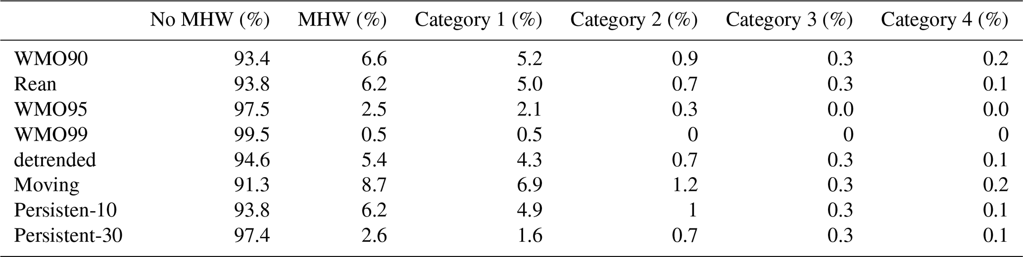
• Percentile effect – Moving from the 90th to the 95th or 99th percentile progressively screened out moderate anomalies and highlighted only the strongest warm events (Figs. 6, 7), and reduced the spatial extent and severity of events (Fig. 7C–D; Table 2).

• Duration effect – Requiring 10 consecutive days (instead of 5) removed shorter MHWs, however only reduced MHW globally by 0.5 % (Table 2). A 30 d minimum isolated only the most persistent basin-scale events globally (Fig. 7), and reduced the extent of MHWs by 4 %. However, for the Pacific Blob there was little effect other than a slight reduction in the spatial extent of low-intensity areas (Fig. 7).

• Detrending effect – After detrending, some events disappeared on a global scale (1.2 % Table 2), making the threshold for MHW detection higher (Fig. 7). However, there was little effect on the Pacific Blob, which highlighted that the event was not due to long-term warming (Bond et al., 2015).

• Baseline choice (WMO vs. Reanalysis) – There was little difference on the global scale between the WMO and reanalysis baselines (0.4 %, Table 2). However, the severity index for the Pacific Blob was generally higher for the WMO baseline than the reanalysis, with a greater extent of category 3 and 4 events (Fig. 7).

• Moving baseline (moving-average) – A rolling 30-year climatology increased the occurrence of MHWs globally by 2.1 % (Table 2). As the thresholds climb with time. As 2014 is closer to the start of the rolling window, comparatively lower thresholds lead to greater MHW occurrences (Fig. 7).

Together, the panels show that the Blob's existence is robust across definitions, but its spatial extent and intensity category vary depending on baseline, threshold and persistence parameters.

Table 2 Summary statistics for area of oceans covered by MHWs alongside categories for different experiments.

5 Data Records and Access

All data described in this paper are provided as CF-compliant NetCDF files and are served through an ERDDAP data server (https://erddap.dmi.dk/erddap, last access: 18 August 2026). ERDDAP lets users download whole files or extract subsets by time, latitude, longitude and variable, in NetCDF, CSV, JSON, MATLAB and other formats, through a point-and-click web interface, direct download URLs, or the rerdapp (R) and erddapy (Python) packages. Each file carries metadata attributes describing its variables, units and conventions.

File types

The database comprises three types of file:

• Daily climatology files: for each grid cell and baseline, the seasonal mean and the 1st, 5th, 10th and 50th percentiles, together with one of the 90th, 95th or 99th percentiles depending on the experiment, plus the corresponding MHW and marine cold-spell (MCS) threshold fields. One file per day-of-year, e.g. 362_Raw_90p_1991-2020_SSTCCI.nc.

• Anomaly files: daily global maps of SST anomaly (observed SST minus the daily climatological mean), for both raw and detrended input and relative to both the fixed and moving climatologies. Daily files span the full record, except that the moving-window products and p95/p99 of the 1993–2022 reanalysis period provide a file only for the last year of each window. One file per date, e.g. 20161227_Raw_5d_90p_1991-2020 _anomalies_SSTCCI.nc.

• Category files: daily categorical severity encoding the MHW or cold-spell category (0 for none, 1–4 for moderate to extreme), based on the highest percentile threshold of each experiment (usually the 90th/10th percentile; 95th/5th and 99th/1st in selected experiments). Coverage matches the anomaly files. One file per date, e.g. 20161227_Raw_5d_90p_1991-2020 _categories_SSTCCI.nc.

Naming and organisation

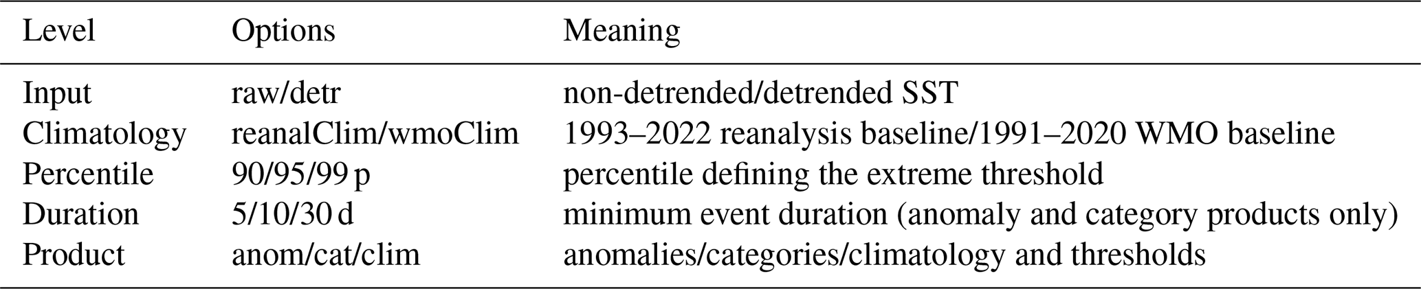
Each product's provenance is encoded both in the directory tree and in a matching ERDDAP dataset identifier, built from the following components in Table 3.

The identifier is assembled as mhw_<input>_<climatology>_<percentile> _<duration>_<product>. For example, the 10 d duration categories computed on raw input against the WMO climatology with a 90th-percentile threshold are identified as mhw_raw_wmoClim_90p_10d_cat. Climatology products are not duration-specific and omit that term (e.g. mhw_raw_reanalClim_90p_clim). The variable to request within each product is anom for anomalies; cat_HW or cat_CS (the heatwave and cold-spell categories) for categories; and the climatological mean, percentile fields (e.g. p90) and threshold fields (threshHW, threshCS) for climatology. The full list of identifiers and variables is shown on the server's home page.

Table 3 Components of the MHW-MAD dataset identifier, showing the options available at each level and their meaning.

Accessing the data

The simplest route is the web interface (Fig. 8). The Data Access Form (Fig. 8) lets a user select a dataset and enter the desired time and latitude/longitude bounds as well as date, and download the subset in the chosen format. It also displays the exact request URL it builds, which can be copied for scripted or repeated use. The “Make A Graph” page (Fig. 9) produces an immediate map.

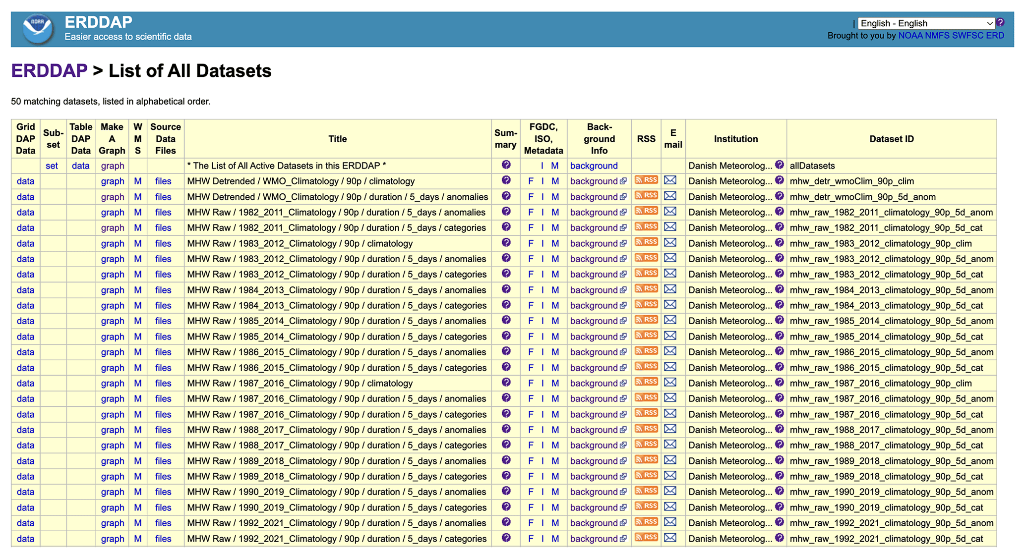
Figure 8 The MHW-MAD database served through the DMI ERDDAP server, with each row a single dataset spanning the raw and de-trended definitions, baselines (fixed, WMO, and rolling 30-year windows), thresholds, durations, and variable groups. Available at https://erddap.dmi.dk/erddap/info/index.html?page=1&itemsPerPage=1000 (last access: 18 August 2026).

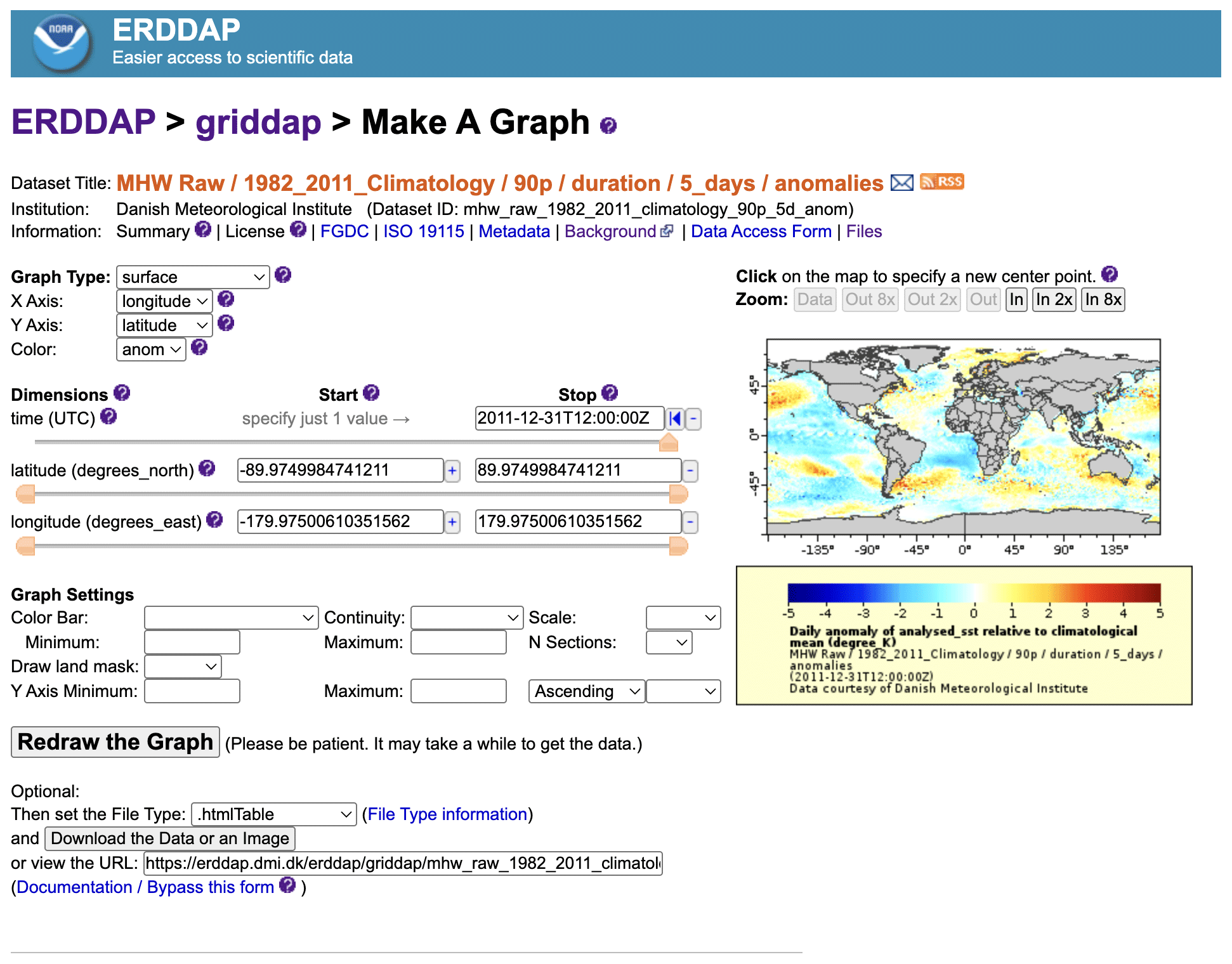
Figure 9 The ERDDAP “Make A Graph” interface for one dataset (raw SST, 1982–2011 baseline, 90th percentile, 5 d minimum, daily anomalies), showing on-the-fly plotting of the SST anomaly and server-side subsetting by date and region. Available at https://erddap.dmi.dk/erddap/griddap/mhw_raw_1982_2011_climatology_90p_5d_anom.graph (last access: 18 August 2026).

Equivalently, any request can be written as a single URL of the form …/griddap/<datasetID>.<format>? <variable>[<time>][<latitude>] [<longitude>]. For example,

https://erddap.dmi.dk/erddap/griddap/ (last access: 18 August 2026)

returns the daily SST anomaly over 1 June–31 August 2023 for the North Sea, the various parts of the URL are shown in Table 4.

Table 4 Components of an ERDDAP griddap request URL, illustrated with the North Sea anomaly example.

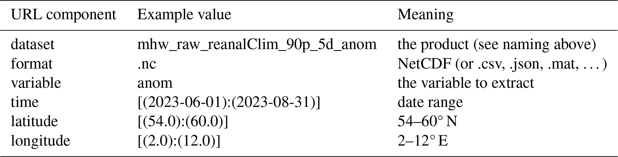
Values given in parentheses select by coordinate value, and setting a range's start and end equal returns a single grid cell. This same North Sea subset can be downloaded from the command line, or with the R and Python clients, as follows:

bash

\# wget

wget -O northsea_anom_2023.nc \

"https://erddap.dmi.dk/erddap/griddap/
mhw_raw_reanalClim_90p_5d_anom.nc?anom
[(2023-06-01):(2023-08-31)][(54.0):
(60.0)][(2.0):(12.0)]"

\# curl
curl -o northsea_anom_2023.nc \
"https://erddap.dmi.dk/erddap/griddap/
mhw_raw_reanalClim_90p_5d_anom.nc?anom
[(2023-06-01):(2023-08-31)][(54.0):
(60.0)][(2.0):(12.0)]"

python

# Python (erddapy)

from erddapy import ERDDAP
e = ERDDAP(server="https://erddap.dmi.
dk/erddap", protocol="griddap")
e.dataset_id = "mhw_raw_reanalClim_90p
_5d_anom"
e.griddap_initialize()
e.constraints = {"time>=": "2023-06-01",
 "time<=": "2023-08-31",
    "latitude>=": 54, "latitude<=": 60,
    "longitude>=": 2, "longitude<=": 12}
ds = e.to_xarray()  # an xarray.dataset
of 'anom'

r

# R (rerddap)

library(rerddap)
info <- info("mhw_raw_reanalClim_90p_
5d_anom", url = "https://erddap.dmi.dk/
erddap/")
d <- griddap(info, time
= c("2023-06-01", "2023-08-31"),
latitude = c(54, 60),
longitude = c(2, 12), fields = "anom")

In the wget and curl calls the URL is quoted because the brackets and parentheses are interpreted by the shell. A user interested in a small study area, a coastal site or even a single grid cell can thereby extract exactly the data they require, removing a common practical barrier to working with large global gridded archives.

6 Usage Notes

6.1 Potential Applications

This database is intended as a resource for a broad range of studies in oceanography, climatology, and marine ecology. For example, researchers examining biological responses to ocean warming events can use the various MHW definitions to test sensitivity. For example, one could correlate coral bleaching occurrences or fishery yields with MHWs defined by the standard vs. a longer-duration criterion. If an impact (such as a coral bleaching event) correlates only with the longer, more intense MHWs, that insight could inform management, for example focusing on multi-week thermal stressors. Our detrended anomalies could also help separate impacts due to anomalous variability from those simply due to overall warming (Amaya et al., 2023). The parallel marine cold spell products further allow ecological responses to both warm and cold extremes to be examined within a single, consistent framework.

6.2 Code Availability

We aim to make this code available as a python package, for users to create their own satellite-based MHW indicators, as such the code is currently under embargo.

7 Summary and Outlook

Here we have presented a comprehensive database that provides a flexible toolkit for studying MHWs at the global scale. As this database enables direct comparisons of MHW characteristics under different definitions, we address a critical need in the field, as divergent definitions have made it difficult to compare results across studies. With our multi-definition framework, researchers can now assess how much of the discrepancy between studies is simply due to the choice of MHW definitions.

Through a brief analysis of our data, we showed that a short or moderate warming event might be classified as an MHW under the less restrictive standard definition of a 90th percentile and 5 d requirement, but would not register under a stricter definition (99th percentile or 30 d minimum). Conversely, what we consider an “extreme” MHW under the standard definition might be fairly routine under a shifting baseline in a warming climate. This has implications for how we interpret long-term trends. Under a fixed baseline, there were more MHWs than with a detrended baseline, consistent with the effect of climate change driving more frequent extremes. Both fixed, moving, and detrended baselines are valid: the fixed highlights the change relative to past climate, and the others highlights deviations from the contemporary climate or long term warming. The database provides both views, and the reality of ocean warming means users should be mindful of which dataset is most appropriate for their studies. For example, whether the biological response of interest is more sensitive to absolute temperatures or to deviations from a shifting mean, or whether an event can truly be considered extreme if its occurrence has become increasingly frequent?

It is worth noting that while our database focuses on surface waters (being SST-based), subsurface MHWs can also occur and may not always align with surface events. Our use of SST CCI means areas of the ocean below the mixed layer are not directly assessed here. Future efforts could merge this with subsurface temperature data or model output to examine the vertical dimension of MHWs. Additionally, the framework here has been applied to marine cold spells, and could be applied to further variables. The general approach of multi-definition analysis is broadly applicable to extreme events research.

Looking ahead, we anticipate updating and expanding this dataset, adding new products and definitions such as non-linear detrending as well as extending persistence thresholds for detrended data. We hope to update the dataset on an annual basis, and to incorporate additional SST products. As new SST reanalysis products or satellite data become available, they can be incorporated to extend the record and possibly improve accuracy in certain regions, for example in coastal and sea ice covered areas. By embracing the complexity of definitions rather than choosing a single metric, it enables a more nuanced understanding of extreme ocean warming events under climate change.

8 Data availability

The MHW-MAD database is archived at Zenodo under https://doi.org/10.5281/zenodo.21835325 (Hayward et al., 2026). The gridded fields exceed the capacity of the repository and are distributed openly by the Danish Meteorological Institute as CF-compliant NetCDF files at https://download.dmi.dk/public/MHW/ (last access: 18 August 2026) and through subsetting, OPeNDAP and WMS services at https://erddap.dmi.dk/erddap/ (last access: 18 August 2026). Both endpoints serve identical files and require no registration, login or access agreement. The Zenodo record provides the persistent identifier for citation together with full documentation and a manifest of all datasets. All data are available under a Creative Commons Attribution 4.0 International licence.

The input sea surface temperature data are the ESA SST CCI Level 4 Analysis product version 3.0, including its interim climate data record extension, available from the NERC EDS Centre for Environmental Data Analysis under the DOI https://doi.org/10.5285/4a9654136a7148e39b7feb56f8bb02d2 (Good and Embury, 2024) and described in Embury et al. (2024). Further information on the initiative and its full range of products is available at https://climate.esa.int/en/projects/sea-surface-temperature/data/ (last access: 18 August 2026). These data are also distributed under a Creative Commons Attribution 4.0 International licence.

9 Conclusions

Our global MHW dataset offers, in a single resource, daily data that span the spectrum of commonly used definitions. As our dataset includes both fixed (1991–2020) and moving 30-year baselines, users can analyse how a warming-adjusted threshold reshapes event counts relative to a historical climate normal. Parallel streams of raw and linearly detrended SST anomalies further allow researchers to disentangle MHWs driven by natural variability from those amplified by the long-term warming trend, an essential capability for attribution studies. Event masks are provided at three intensity thresholds (90th, 95th and 99th percentiles) and at three minimum-duration criteria (5, 10 and 30 consecutive days), capturing everything from moderate, short-lived anomalies to the most persistent and extreme episodes. Symmetric marine cold spell products extend the same framework to cold extremes. By packaging these options side-by-side, the dataset becomes both a practical tool for climate monitoring, ecosystem-impact assessments, and a conceptual lens through which to examine how methodological choices alone can alter our perception of ocean extremes. In short, the multi-definition design promotes transparent, apples-to-apples comparisons across studies and supplies a robust foundation for deeper, more nuanced understanding of MHWs in a rapidly changing climate.