Correction of the Observatoire Haute Provence electrochemical concentration cell (ECC) ozonesonde long-term data record over the 2002–2007 period

The Observatoire Haute Provence (OHP) station is one of the few long-term measuring stations for vertical ozone profiles in southern Europe. Since 1991, vertical ozone distribution has been monitored by the OHP weekly electrochemical concentration cell (ECC) ozonesonde. In this study, we have corrected the ECC datasets for the period 2002–2007. The correction of the ECC has been carried out using comparisons with other ozone-measuring instruments at the same station (stratospheric lidar and Système d'Analyse par Observation Zénithale (SAOZ) photometer) and with collocated satellite observations of the ozone vertical profile by Aura-Microwave Limb Sounder (MLS). Median ozone concentration of the ECC for the period 2002–2007 was −3.4 % lower than that of the stratospheric lidar and MLS. The ECC internal pump temperature showed a sudden drop of 16 K at 25 km for the period 2002–2007 compared to the period 1991–2001. Considering the long-term trends of the ECC current and stratospheric lidar ozone concentration at 25 km as well as the ECC pump flow rate trend, we show that the recorded ECC pump temperature between 2002 and 2007 is too low by 10 K at 25 km. The ECC pump temperature for the period 2002–2007 has been corrected using a linear altitude-dependent increasing rate of 0.33 K km⁻¹. As a result, the corresponding ECC ozone bias at 25 km with the stratospheric lidar and MLS have been reduced to −0.5 %. The corrected OHP ECC data are available at https://doi.org/10.25326/855 (Ancellet and Godin-Beekmann, 2025).

1 Introduction

The stratospheric ozone layer recovery is expected due the decline of ozone-depleting substances (ODSs) following the Montreal Protocol and its amendments (WMO, 2023). In the upper-stratosphere (above 35 km), ozone increase has been confirmed by various studies (e.g. Godin-Beekmann et al., 2022; Petropavlovskikh et al., 2025; Steinbrecht et al., 2017). The monitoring of ozone in the upper troposphere and lower stratosphere (UTLS) region is crucial for Earth's radiation budget (e.g. Riese et al., 2012) and for modulating air quality near Earth's surface via deep stratospheric intrusions (e.g. Lin et al., 2015). Despite its importance, the confidence in the long-term ozone trends in the UTLS remains low (Godin-Beekmann et al., 2022; Petropavlovskikh et al., 2025; Steinbrecht et al., 2017; Van Malderen et al., 2021). The longest records of the vertical ozone distribution in the stratosphere are provided by balloon borne ozonesondes regularly launched at more than 50 stations around the world. An ozonesonde is a small and lightweight instrument that measures atmospheric ozone profiles up to about 30–35 km (Komhyr, 1969; Komhyr et al., 1995). The ozone measurement is based on the electrochemical method where ozone is titrated in a potassium iodide (KI) sensing solution. The chemical transformation generates an electric current proportional to the amount of ozone; hence the name electrochemical concentration cell (ECC). Data of many ozonesonde stations were recently reprocessed to reduce uncertainties in ozone trends (Ancellet et al., 2022; Sterling et al., 2018; Tarasick et al., 2016; Van Malderen et al., 2016; Witte et al., 2017, 2018), but some instrumental artifacts still need to be addressed at some stations (Smit and Thompson, 2021). The homogenization of the ozonesonde records followed the Ozonesonde Data Quality Assessment (O3S-DQA) panel recommendations (Smit et al., 2012). At the Observatoire de Haute Provence (OHP: 43.93° N, 5.71° E), ozone vertical profile monitoring has been carried out since the mid-1980s by ozonesondes and lidar observations. The OHP is one of the few long-term measuring stations for vertical ozone profiles in Southern Europe. Improvement and homogenization of the ECC ozone observations at OHP from 1991 to 2021 has been detailed in Ancellet et al. (2022). However ECC total columns after homogenization still show underestimated values for the 2005–2007 period when looking at comparisons with satellite observations (Fig. 9 in Ancellet et al., 2022). Therefore detailed comparisons of OHP ECC profiles with lidar and Microwave Limb Sounder (MLS) observations are needed in the stratosphere. This paper begins with an overview of the ozonesonde measurement system, and brief descriptions of stratospheric lidar and the MLS data in Sect. 2 followed by a comparison of ozone concentrations between ozonesonde and collocated lidar/MLS records in Sect. 3. The reprocessing approach and methodology are described in Sect. 4. The analyses that compare the original and reprocessed time series are also described. The conclusion appears in Sect. 5.

2 Data

2.1 Ozonesonde

ECC ozonesondes have been used in OHP since 1991 to measure ozone vertical profiles on a weekly basis (generally around 09:00 UT). ECC generates an electrical current through the reaction of ozone in a KI solution. The ozone partial pressure $P_{{\mathrm{O}}_{\mathrm{3}}}$ (measured in mPa) is then obtained from the electrochemical current I_M (measured in µA), the background current I_B measured in the preparation laboratory with an ozone removal filter after the sonde was exposed to ozone, the gas volume flow rate Φ_P (in cm³ s⁻¹) of the air sampling pump, the pump temperature T_P (in K) and the total efficiency of the ozone sensor η_T (Smit and Thompson, 2021).

$$\begin{array}{}\text{(1)}& P_{{\mathrm{O}}_{\mathrm{3}}}={\displaystyle \frac{\mathrm{4.306}\times {\mathrm{10}}^{-\mathrm{2}}{T}_{\mathrm{P}}}{{\mathit{\eta }}_{\mathrm{P}}{\mathit{\eta }}_{\mathrm{A}}{\mathit{\eta }}_{\mathrm{C}}{\mathrm{\Phi }}_{\mathrm{P}}}}(I-I_{\mathrm{B}})\end{array}$$

The total efficiency η_T consists of pump flow efficiency η_P, absorption efficiency η_A and conversion efficiency of the absorbed ozone η_C. The median value of the relative uncertainty in the ozone concentration measured by the ECC is on the order of 6 %–7 % in the stratosphere (Ancellet et al., 2022). Total column ozone (TCO) measurements by the UV-visible SAOZ (Système d'Analyse par Observation Zénithale) and the Dobson spectrophotometer are available at OHP. The so-called normalization factor is calculated as the ratio of the spectrophotometer TCO and the ECC TCO. Historically, ozonesonde profiles have often been normalized or scaled to an independent measurement of the TCO. Normalization of ECC sonde profiles is no longer recommended, however the normalization factor provides a useful indicator for the quality of ozonesonde profile data and the consistency in ozonesonde data time series. We use the dataset of the Dobson spectrophotometer from 1991 to 2004 and of the SAOZ from 2004 to 2023 to calculate normalization factor. The residual ozone above the 10 hPa pressure altitude or above the balloon burst altitude is derived from the McPeters and Labow (2012) satellite monthly mean climatology. The normalization factor is not calculated for balloon burst altitude lower than the 25 hPa pressure level or when the SAOZ measurement is not available. The corresponding sounding are nevertheless included in the OHP data set. This corresponds to 9.5 % of the 1524 OHP soundings from 1991 to 2023. Only ozonesonde profiles with a normalization factor below 1.3 are considered here (i.e. only 3 soundings out of the 1524 are excluded of the data base). The fraction of soundings with normalization factor higher than 1.2 is 1.3 %. Normalization factor are always larger than 0.83 and no filtering is applied for low values of the normalization factor.

The details of instrument changes and the homogenization are described in Ancellet et al. (2022). Briefly, the main changes considered in this work are as the following: a major change in the sounding procedure occurred in March 1997 when the Science Pump Corporation (SPC) ozonesonde was replaced by the Environmental Science Corporation (EnSci) ozonesonde. In July 2007, the radiosonde type switched from Vaisala RS80 to Modem M10, together with a change of the position of pump temperature inserted in the pump hole instead of being taped to the pump. The TMAX electronical interface between the radiosonde and the ECC changed in 2002. As far as we know from available written information from this time period no other significant changes of the sounding preparation occurred during the time period March 1997 and July 2007. Correction of pump temperature has been implemented in Ancellet et al. (2022) to account for the changes in the position of the ECC pump thermistor in June 2007. However the homogenized ECC pump temperature T_P remains inhomogeneous for the the period 1991–June 2007 and this correction must be carefully assessed. In this work, the ECC pump temperature correction is assessed by comparison of homogenized ECC ozone concentrations with other ozone measurements obtained at OHP in as close coincidence as possible.

2.2 Lidar

At OHP, regular nighttime measurements (2–4 per week) by the Differential Absorption Lidar (DIAL) ozone lidar have been made since 1985 (Godin-Beekmann et al., 2003). The lidar is optimized for stratospheric ozone profiling between 10 and 50 km a.s.l. using an absorbed laser wavelength at 308 nm and a reference laser wavelength at 355 nm. Ozone profiles are obtained during the night in clear sky conditions and over a time range of 4 h. The best accuracy (5 %) is generally obtained in the 15–40 km altitude range where ozone concentrations are large enough to minimize lidar systematic errors and signal-to-noise ratio (SNR) is maximum (Nair et al., 2011; Wing et al., 2020). The coincidence is determined with a temporal criterion of ±12 h of the ECC sonde launch time for the comparison.

2.3 MLS

The Microwave Limb Sounder (MLS) on-board the Aura satellite, launched on 15 July 2004, measures vertical profiles of the abundances of key atmospheric species, including ozone. We use Aura MLS level 2 version 5.0x ozone volume-mixing ratio vertical profile observations (Schwartz et al., 2021) for a comparison with the ECC ozonesonde time series. The accuracy from 68 to 4.6 hPa is 5 %–8 % (Livesey et al., 2022). The coincidence with the ECC sonde launch is determined with spatial differences less than ±2.5° latitude and ±8° longitude, and temporal differences less than ±12 h. Using a smaller domain would significantly decrease the number of coincidences. Data screening based on the recommended values of the status flag, quality field and convergence field have been applied to the MLS data selected for the analysis of the stratospheric ozone profiles above OHP.

3 Comparison of ECC ozone concentrations with MLS and lidar

The monthly mean ozone concentrations of the ECC ozonesonde and the stratospheric lidar are compared for a layer of 2 km thickness centered at 25 km (Fig. 1a). Monthly mean differences between ECC and lidar ozone concentrations are shown in Fig. 1c with frequent occurrences of negative differences before 2007. The median relative difference is −4.6 % for the period January 2002–June 2007, while the mean relative differences are −3.3 % and −0.3 % for the period March 1997–December 2001 and July 2007–December 2023, respectively (Fig. 1c). Considering coincident measurements within ±12 h, the difference between the ECC ozonesonde and the lidar for the period January 2002–June 2007 can be reduced (Fig. 1b and d). The median relative difference is nevertheless as large as −3.4 % for the period January 2002–June 2007, while the mean relative differences are −2.0 % and 0.1 % for the period March 1997–December 2001 and July 2007–December 2023, respectively (Fig. 1d). The two times standard error on the median value is less than 1.5 %. So the bias is still significant for the period January 2002–June 2007.

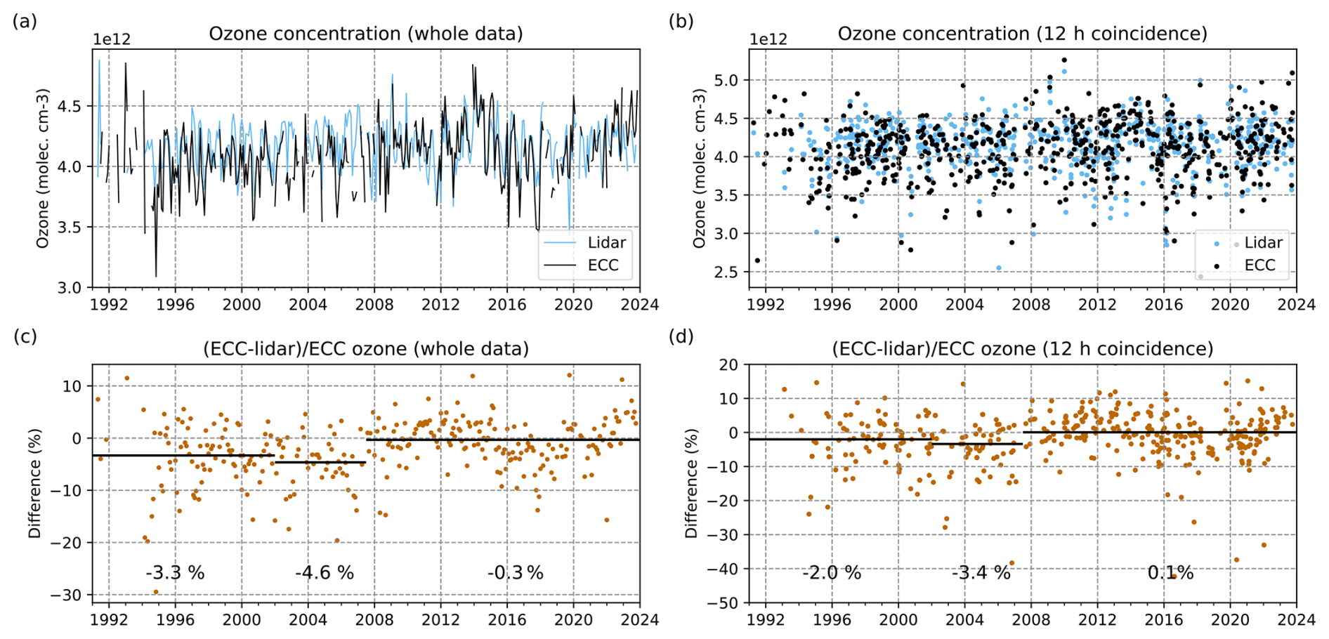
Figure 1 Time series of the ozone concentration of the stratospheric lidar and the ECC ozonesonde at 25 km. Ozone concentrations are calculated at altitude 25 km by averaging ozone over a range of ±1 km. (a) Monthly mean and (c) mean relative ECC minus lidar ozone concentration differences (in %). Monthly means are calculated for the months which the number of observations in each month is greater than or equal to 3. (b) Ozone concentration and (d) relative ECC minus lidar ozone concentration differences for the coincident (<12 h) profiles. Black lines with values in (b) and (d) indicate median relative differences for three periods: January 1991–December 2001, January 2002–June 2007 and July 2007–December 2023.

We have also compared ozone concentrations between the ECC ozonesonde and MLS at 26.1 hPa for the period January 2005–December 2023 (Fig. 2). The median relative difference for the period January 2005–June 2007 is also −3.4 % which is larger than that for the period July 2007–December 2023 (Fig. 2b). The two times standard error on the median value being now as large as 4.0 %. The ECC ozone bias remains significant (p < 0.05) according to the Wilcoxon rank sum test (Wilcoxon, 1945) when considering differences with MLS for the period January 2002–June 2007. The sign of the bias is similar to the results obtained when comparing ECC and lidar for the period 2002–2007. Therefore, we investigated the cause of the underestimation based on Eq. (1) and the statistical distributions of the parameters used to calculate the partial pressure of ozone.

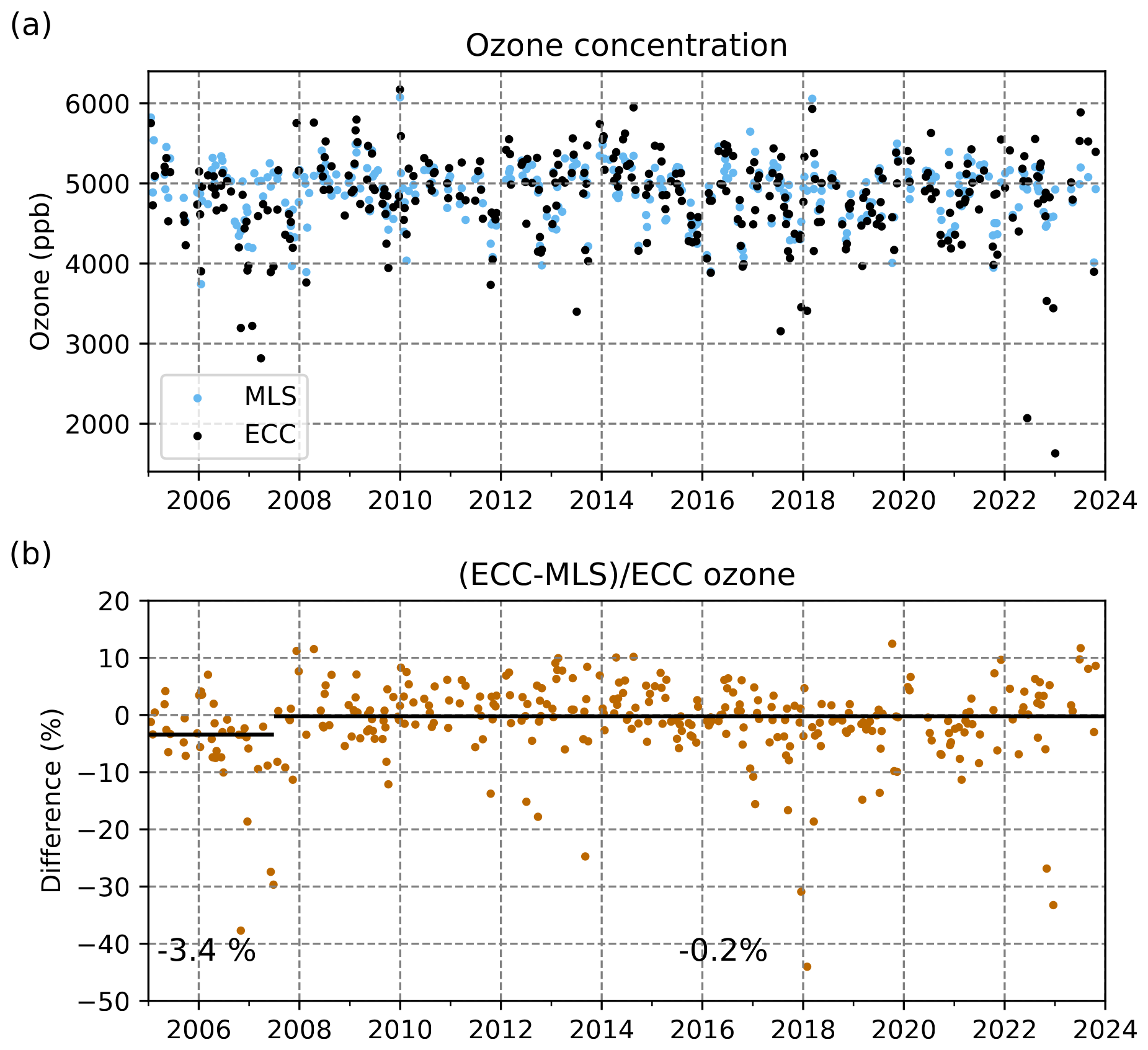
Figure 2 Time series of the ozone concentration of MLS and the ECC ozonesonde at 25 km. Ozone concentrations are calculated at pressure level 26.1 hPa by averaging ozone over a range of ±1 km layer (31.6–21.5 hPa). (a) Ozone concentration and (b) relative ECC minus MLS ozone concentration differences (in %) for the coincident (<12 h) profiles. Black lines with values in (b) indicate median relative differences for three periods: January 1991–December 2001, January 2002–June 2007 and July 2007–December 2023.

4 Results and discussion

4.1 Time evolution of ozonesonde parameters

ECC pumping time for 100 mL of air is expected to change especially when switching ECC type or motor power supply. Its time evolution is shown in Fig. 3. There is indeed lower pumping time values from 2002–2007 in the range 27–29 s. However these values are within the 25–35 s recommended values in Smit and Thompson (2021). The time evolution shown in Fig. 3 is taken into account in the ozone calculation using Eq. (1) and OHP metadata records are very reliable for this parameter. Therefore we do not expect the low ozone values observed at 25 km to be caused by incorrect values of the ECC flow rate used in the data processing.

Stauffer et al. (2022) reported that EnSci ECC total ozone column drop occurring at selected sites after 2013 could be related to ozonesonde production changes as well as station-specific factors due to ozonesonde preparation. The ECC serial numbers associated with sounding exhibiting TCO decreases larger than 3 %–5 % were above 20 000. The EnSci serial numbers are between 6200 and 12 800 for the OHP soundings made between January 2002 and June 2007. We therefore cannot identify a clear connection with the sonde production quality discussed in that paper.

ECC internal pump temperature, T_P, correction is another key factor in calculating ozone partial pressure since the correction of ECC pump temperature applied in Ancellet et al. (2022) can be as large as 10 K to account for wrong thermistor position. Figure 4 shows its time evolution with three periods showing changes in the range of the homogenized ECC pump temperature (in this work the measured ECC pump temperature always refers to the homogenized ECC temperature retrieved in Ancellet et al., 2022). Overall, values are in the range 290–300 K after June 2007 while they are in the range 300–310 K before January 2002. The latter could be explained by a major change of the ECC installation in the Styrofoam box when switching from Vaisala RS80 to Modem M10 (new electronic interface and new batteries). However, the homogenized pump temperature frequently dropped within the range 280–290 K between January 2002 and July 2007 without a clear explanation for such a negative drop. The 8 K temperature positive correction in the stratosphere due to the position of the thermistor being taped instead of being inserted in the pump hole before July 2007 has been applied to all the sondes from January 1991 to June 2007 in Ancellet et al. (2022). The unusually low values of the ECC pump temperature in the January 2002–June 2007 period corresponds to that of the ozone concentration observed in Sect. 3. An additional correction of the ECC pump temperature measurement for this time period might be needed. Other factors, namely, ozone concentration change in the stratosphere and the statistical distribution of the pump flow rate or the ECC current must be taken into account before we apply such correction.

Figure 3 Time evolution of the ozonesonde time in s for pumping 100 mL. The black vertical bar correspond to changes in sondes type or processing software (see Fig. 4). The horizontal red lines are the median values of the pumping time used in Fig. 6, Tables 1, 2.

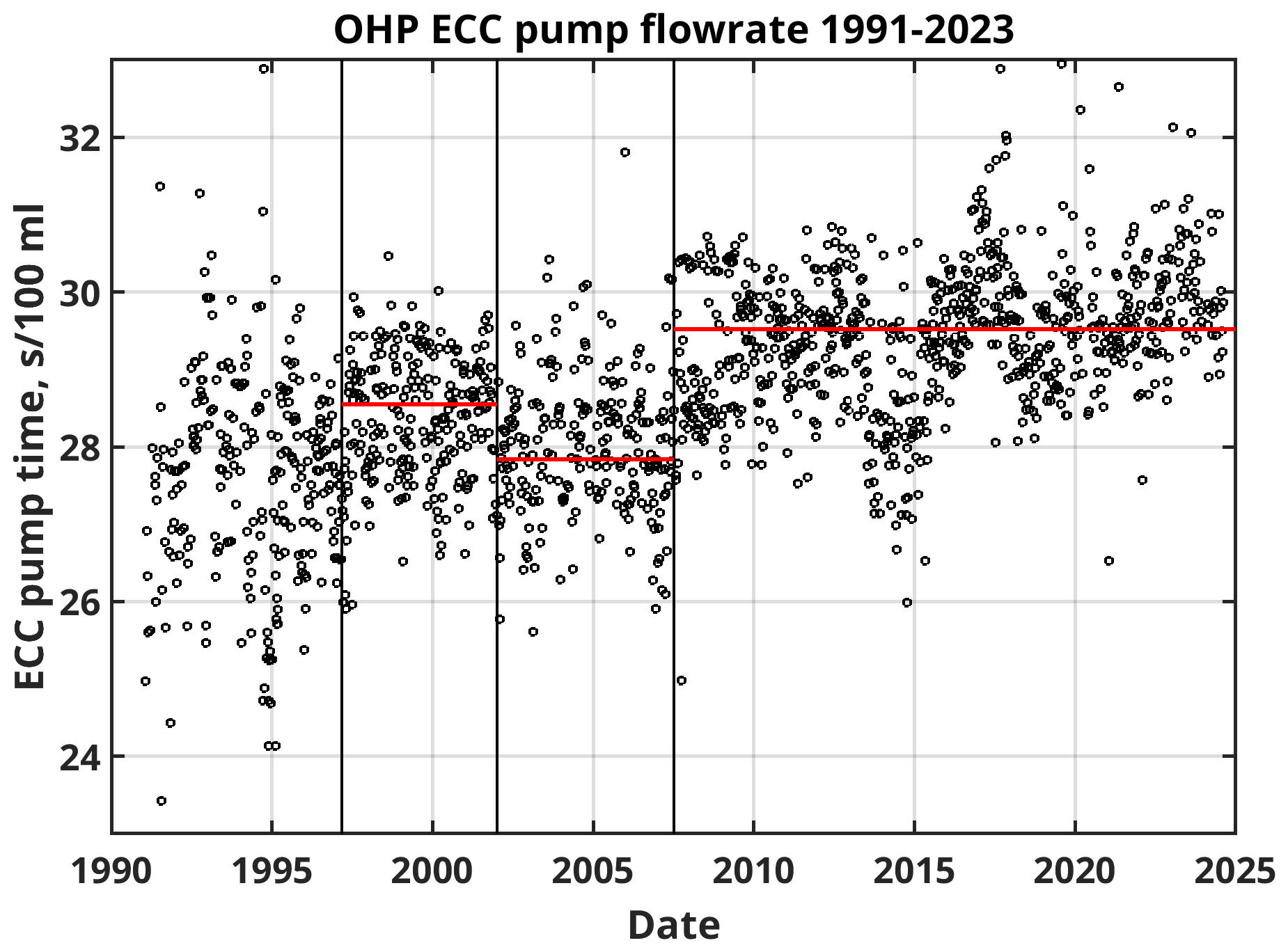
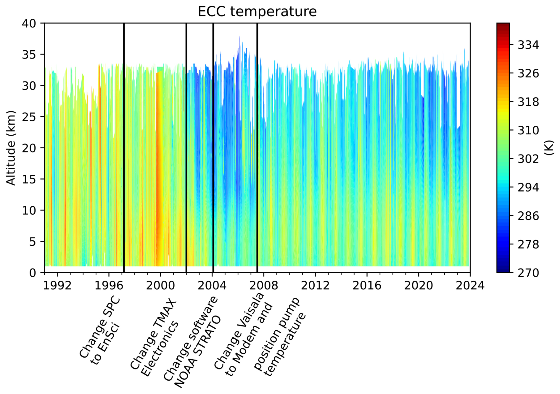
Figure 4 Time evolution of the ozonesonde homogenized internal pump temperature in K as a function of altitude. Major changes of the ECC instrument are shown in the bottom part of the figure.

First, the mean vertical distribution of the homogenized ECC temperature and of the ECC current for three periods (1991–2001, 2002–2007, 2008–2019) are shown in Fig. 5 to emphasize that the ECC temperature drop in 2002–2007 increases with altitude in the stratosphere as does the difference between internal and external ECC pump temperature shown in the analysis of Smit et al. (2012). The differences of ECC current between 2002–2007 and 1991–2001 does not show a clear altitude dependency with no evidence of lower current difference at 30 km than at 20 km in 2002–2007 as we might expect if the ECC solution temperature is so cold that it becomes frozen. In fact the relative differences of ECC current between 2002–2007 and 1991–2001 are −5.4 % at 20 km, −5.7 % at 25 km and −6.8 % at 30 km. Wrong values of the recorded ECC pump temperature in 2002–2007 would thus remain as the possible primary cause of the negative ECC ozone concentration bias in the stratosphere.

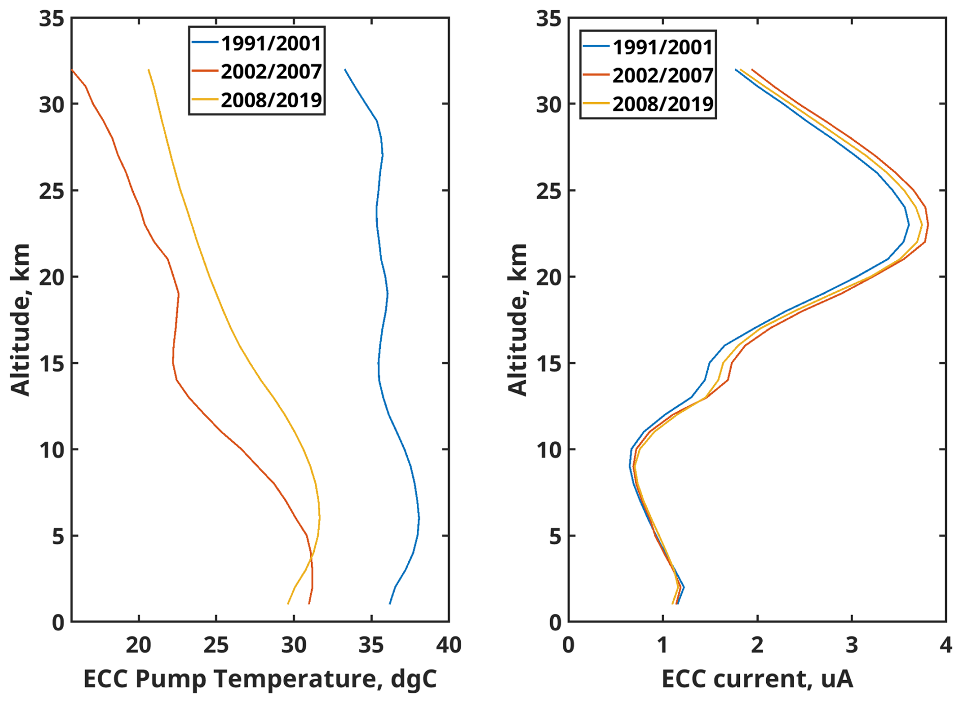
Figure 5 Mean vertical profile of homogenized ECC pump temperature in °C (left panel) and ECC current in µA (right panel) for period 1991/2001, 2002/2007 and 2008/2019.

Second, to check the magnitude of the ECC temperature drop for the period January 2002–June 2007 necessary to explain the ECC ozone concentration decrease at 25 km, the homogenized ECC temperature drop T_P has been compared with a ECC temperature drop T_Pc calculated by using measured ECC current, pump flow and ozone concentration based on the Eq. (1). The ozone concentration measured by the stratospheric lidar at OHP is employed assuming that it is the best proxy to account for any long term ozone change in the stratosphere. We consider three periods: March 1997–December 2001 as period 1, January 2002–June 2007 as period 2 and July 2007–December 2023 as period 3 in this analysis. We did not use the data before March 1997 to avoid considering a change of the efficiency of the ozone sensor η_T when changing the type of ozonesonde in March 1997. The distributions and medians of the ECC temperature T_P, the ECC current, the pump flow and the ozone concentration of lidar are shown in Fig. 6 and Table 1 at 25 km. The differences of ozone concentration observed by lidar among three periods are small (0 %–1 %).

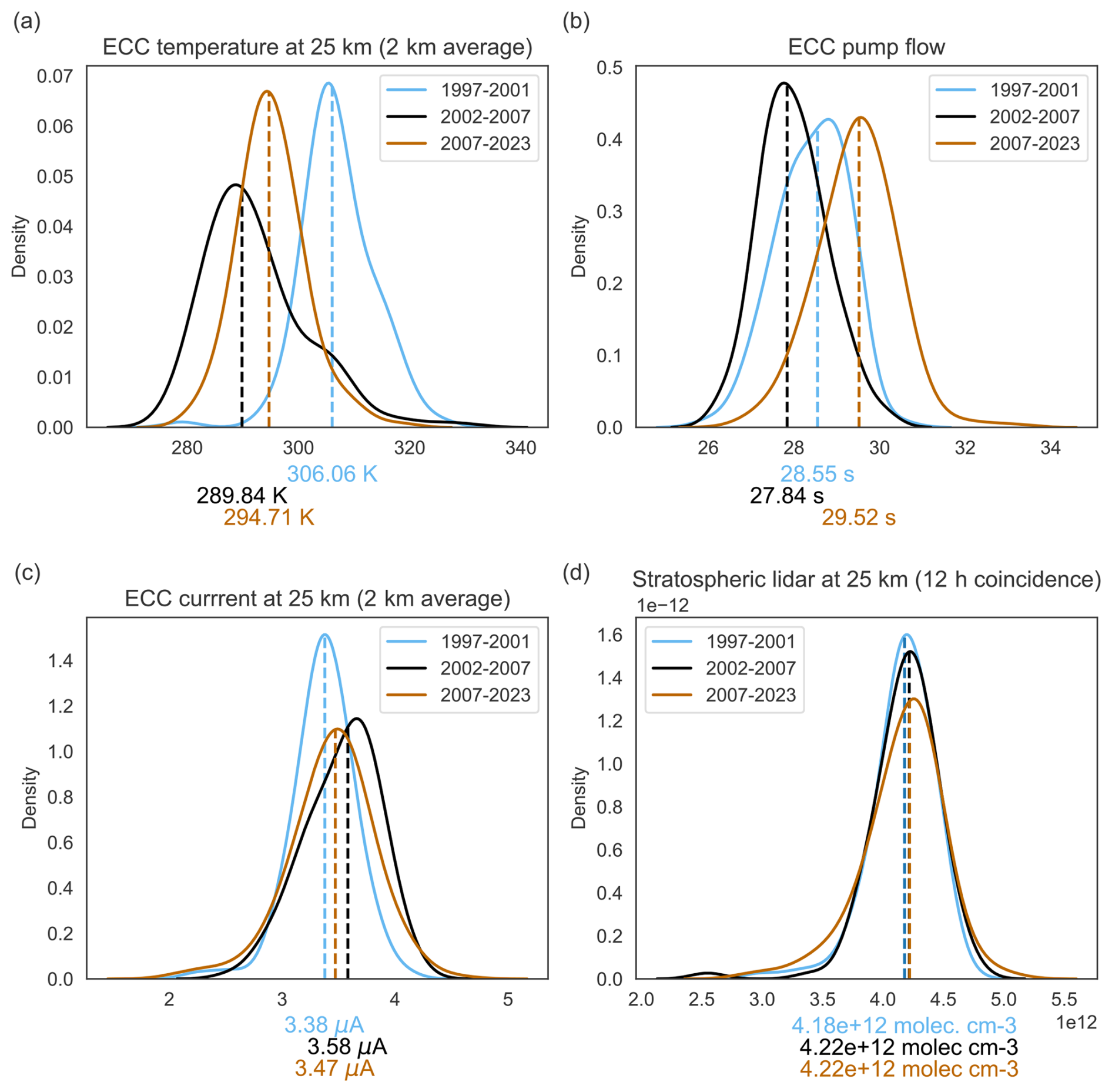
Figure 6 Density plot of the key factors in calculating the ozone partial pressure. (a) ECC homogenized temperature T_P at 25 km in K, (b) ECC pumping time for 100 mL in s, (c) ECC current at 25 km in µA, and (d) ozone concentration in molecule cm⁻³ measured by the stratospheric lidar at OHP for three periods: March 1997–December 2001 (light blue), January 2002–June 2007 (black) and July 2007–December 2023 (brown). The dashed lines and values in the bottom part of figures show medians summarized in Table 1.

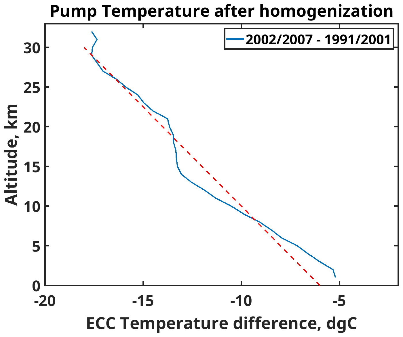
Figure 7 Vertical profile of the mean homogenized ECC pump temperature difference in K between period 2002/2007 and period 1991/2001. The red dotted line shows a linear altitude-dependent correction with an increasing rate of 0.4 K km⁻¹.

Table 1 Medians of the homogenized ECC temperature, the ECC current, the ECC pumping time and the ozone concentration measured at 25 km by the stratospheric lidar for three periods: March 1997–December 2001, January 2002–June 2007 and July 2007–December 2023.

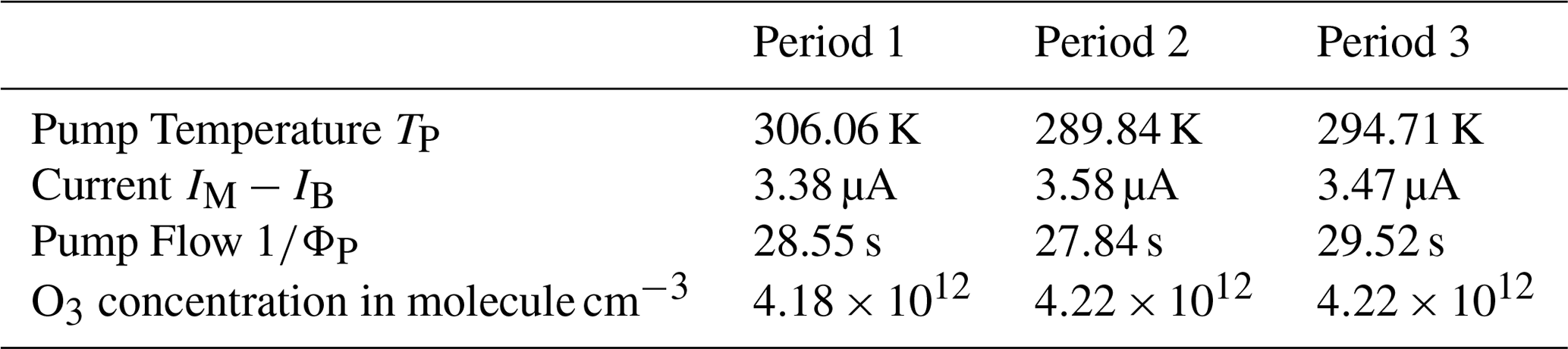
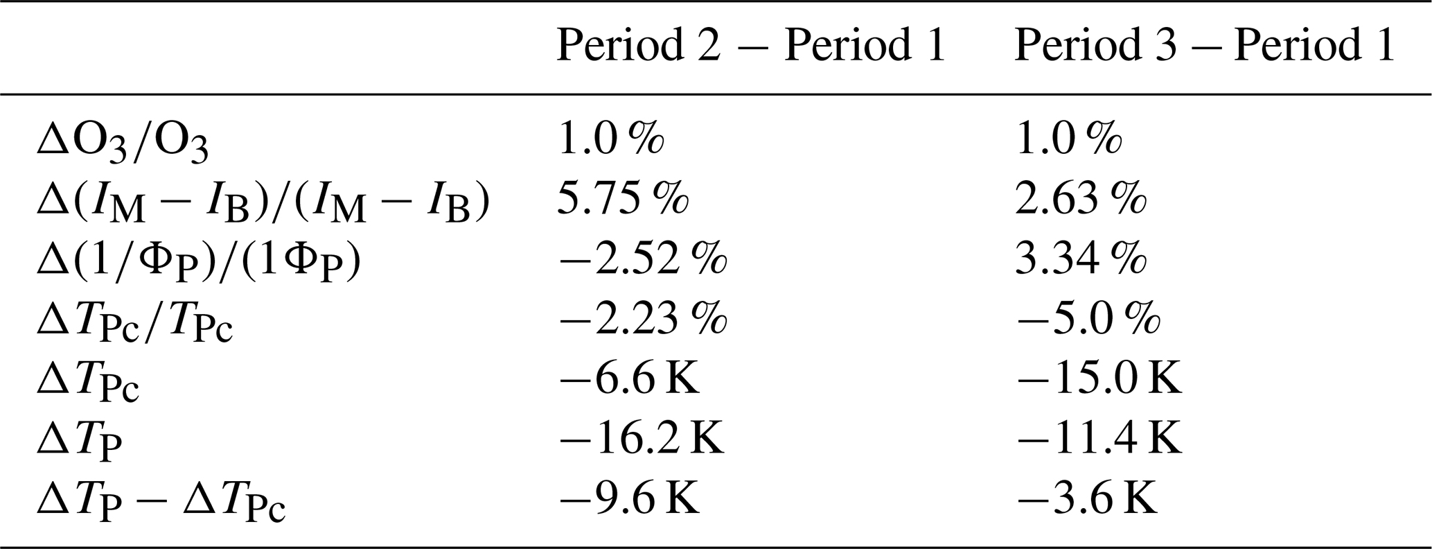
Table 2 Differences of calculated pump Temperature ΔT_Pc using differences of measured current Δ(I_M−I_B), pumping time $\mathrm{\Delta }\mathrm{1}/\mathrm{\Phi }$ and ozone concentration by lidar ΔO₃ at 25 km for three periods: March 1997–December 2001, January 2002–June 2007 and July 2007–December 2023. The calculated pump Temperature difference ΔT_Pc is compared with the homogenized pump Temperature difference ΔT_P.

The calculated percentage difference of homogenized ECC temperature derived from observed differences of ECC current and pump flow rate can be expressed as:

$$\begin{array}{}\text{(2)}& {\displaystyle \frac{\mathrm{\Delta }{T}_{\mathrm{Pc}}}{T_{\mathrm{Pc}}}}={\displaystyle \frac{\mathrm{\Delta }{\mathrm{O}}_{\mathrm{3}}}{{\mathrm{O}}_{\mathrm{3}}}}-{\displaystyle \frac{\mathrm{\Delta }(I_{\mathrm{M}}-I_{\mathrm{B}})}{(I_{\mathrm{M}}-I_{\mathrm{B}})}}-{\displaystyle \frac{\mathrm{\Delta }(\mathrm{1}/{\mathrm{\Phi }}_{\mathrm{P}})}{(\mathrm{1}/{\mathrm{\Phi }}_{\mathrm{P}})}}\end{array}$$

Taken period 1 as a reference percentage differences of all the parameters used in Eq. (2) are shown in Table 2 using measured values of period 2 and 3, i.e. when ozone underestimate change from −3.4 % to 0.1 %. Measured and calculated difference of the mean pump temperature is not large for period 3 (< 4 K) while the difference can be as large as −10 K for period 2.

4.2 Analysis of the 2002–2007 ECC homogenized temperature drop in 2002–2007

Before we present the selected correction procedure of the ECC pump temperature it is important to review the known changes during this time period. First, there was a change of the electronics interface between the ECC and the radiosonde in January 2002 switching from TMAX-HMOS to TMAX-C. An update of the software to read the binary files was made to handle the dataframe from the TMAX-C interface but documentation about this step has been lost. We cannot exclude a bug in the implementation of this software. The use of the TMAX-C interface was discontinued in July 2007 when Modem radiosondes replaced the VAISALA radiosondes.

Second, we make the hypothesis that the thermistor was taped to the pump during this time period 2002–2007 in Ancellet et al. (2022) but this information has not been precisely recorded in the metadata and there is a large uncertainty about the position of the thermistor position in the styrofoam box. The pump temperature correction applied during the homogenization process performed in Ancellet et al. (2022) might not be correct.

Third, the NOAA STRATO version 8.66 has been implemented at OHP to produce level 1 files between February 2004 and June 2007 with two consequences: (i) a different processing software has been applied for the ozone retrieval without a recording of the ECC current in the level-1 files, (ii) the binary files with the ECC current have been lost. In order to include cell current in the data files, Ancellet et al. (2022) performed a reverse calculation of cell current since the necessary variables to back-calculate the cell current from the ozone partial pressure were available in the data file. We are confident that this process produced very small uncertainties in the ECC current retrieval. Use of the STRATO software has been discontinued in July 2007 when switching to the Modem data acquisition system.

4.3 ECC pump temperature correction

The vertical profile of the pump temperature difference between the period 2002–2007 and the period 1991–2001 can be approximated by a linear evolution of −0.4 K km⁻¹ (Fig. 7). We do not expect a perfectly linear altitude-dependent difference since atmospheric temperature profiles cannot be strictly identical for the two periods. The jump at 10 km in the pump temperature difference indeed corresponds to changes in the tropopause altitude. Several ECC pump temperature linear altitude-dependent corrections were therefore tested for the period January 2002–June 2007 in this section. Since according to Sect. 4.1, bias of the ECC pump temperature can be as large as −10 K in period 2 at 25 km, the additional correction applied to the homogenized ECC temperature T_Pcor is calculated as:

$$\begin{array}{}\text{(3)}& T_{\mathrm{Pcor}}\left(z\right)=T_{\mathrm{P}}\left(z\right)+\mathit{\alpha }z\end{array}$$

where z is altitude (measured in km) and α the increasing correction coefficient in K km⁻¹. Since we do not have a clear explanation for the pump temperature drop off in 2002–2007 in the stratosphere, we decided to test three corrections: α=0.17 K km⁻¹ (ΔT_P=0 K at 0 km and ΔT_P=5 K at 30 km) called version 2, α=0.33 K km⁻¹ (ΔT_P=0 K at 0 km and ΔT_P=10 K at 30 km) called version 3 and α = 0.50 K km⁻¹ (ΔT_P=0 K at 0 km and ΔT_P=15 K at 30 km) called version 4. The homogenized ECC temperature without an additional correction is called version 1. The best correction will be chosen first by using the ECC/lidar and ECC/MLS comparisons at 25 km. Four time evolutions of corrected ECC temperature are displayed in Fig. 8. We can see that the observed drop of ECC temperature for the period January 2002–June 2007 is improved in version 3 and version 4.

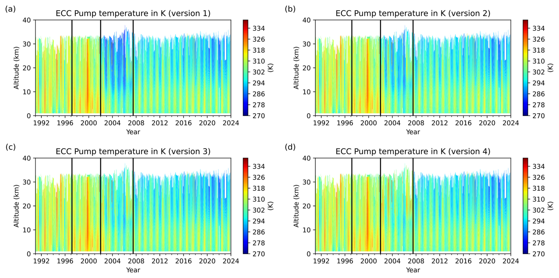
Figure 8 Time evolutions of homogenized pump temperature T_P as a function of altitude. (a) Version 1 Uncorrected values (b) Version 2 corrected values with α=0.17, (c) Version 3 with α=0.33 and (d) Version 4 with α=0.50 in Eq. (3) for the period January 2002–June 2007.

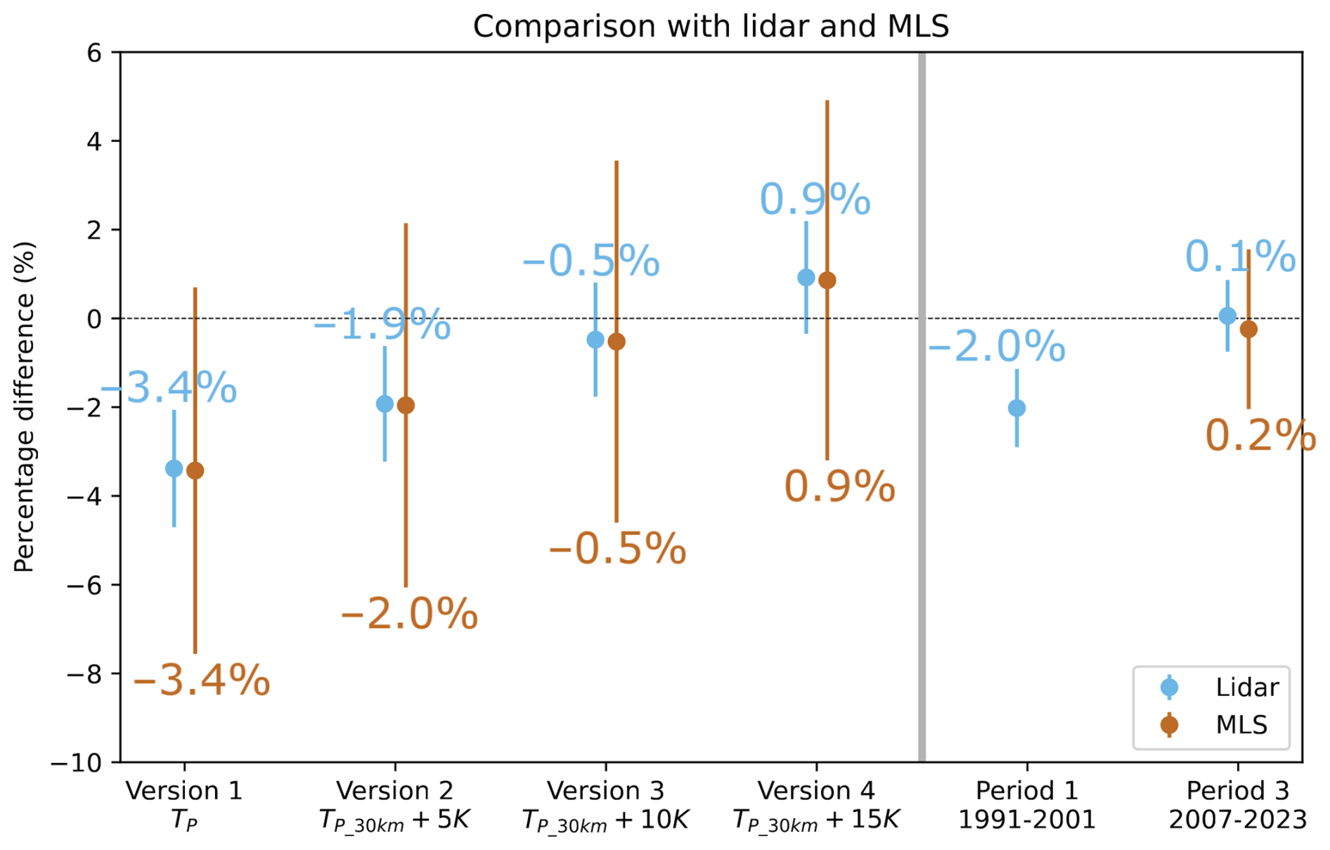
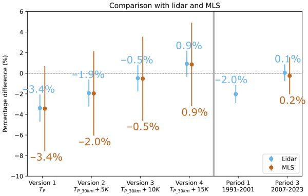
Figure 9 Evaluation of ECC ozone concentration compared with lidar and MLS ozone concentrations. Results are presented as medians and 2× standard errors of percentage difference for a corrected and two uncorrected periods. An uncorrected and three corrected ECC ozone concentrations are tested for the period January 2002–June 2007.

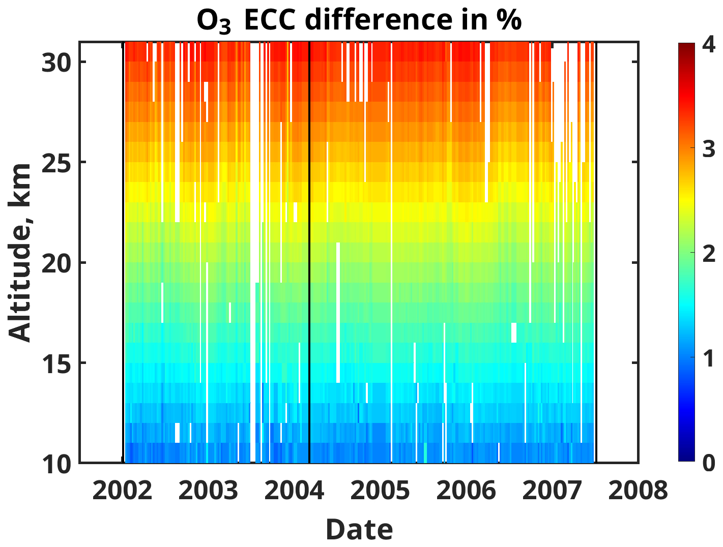
Figure 10 Differences between the ozone concentration calculated without any correction of the homogenized ECC temperature (Version 1 of T_Pcor) and with Version 3 of T_Pcor as a function of altitude for the time period 2002–2007.

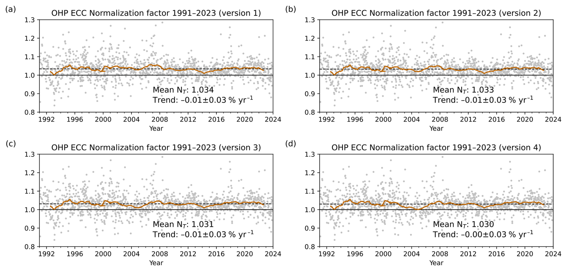
Figure 11 Time evolution of the ECC normalization factor. The dashed black lines are averages of normalization factors for the period January 1991–December 2023. The thick brown lines are the 100-point, centered, moving averages.

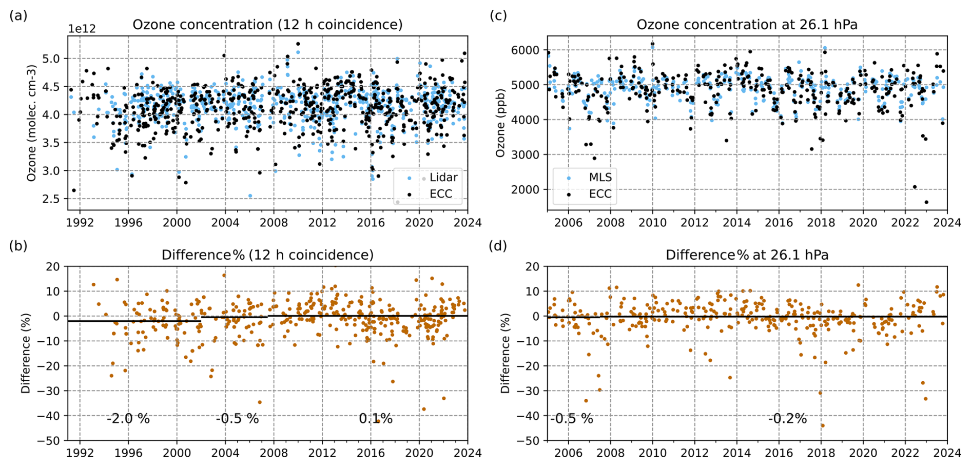
Figure 12 Time series of ozone concentration of the stratospheric lidar and the ECC ozonesonde at 25 km, and MLS and the ECC ozonesonde at 26.1 hPa (a, c). Ozone concentration and (b, d) relative ECC minus lidar ozone concentration differences for the coincident (< 12 h) profiles. Ozone concentrations for (a)–(b) are calculated at altitude 25 km by averaging ozone over a range of ±1 km. Ozone concentrations for (c)–(d) are calculated at pressure level 26.1 hPa by averaging ozone over a range of ±1 layer (31.6–21.5 hPa). Black lines with values in (b) and (d) indicate average relative differences for the periods same as Figs. 1–2.

To compare with the ozone concentrations of the stratospheric lidar and MLS, ozone concentrations are calculated by using three corrected ECC temperatures. Originally, median ozone concentration of the ozonesonde at 25 km for period 2 shows −3.4 % lower compared with those of the lidar and MLS (Figs. 1d and 2b). Ozone concentration corrected by the ECC temperature version 2 is still −2.0 % lower (Fig. 9). The ECC correction version 3 (ΔT_P=0 K at 0 km and ΔT_P=10 K at 30 km) should reproduce ozone concentration which is equivalent to that of the stratospheric lidar according to Table 2. The ECC median ozone concentration corrected by the ECC temperature version 3 is −0.5 % lower than the lidar median ozone concentration during the period 2 (January 2002–June 2007). This −0.5 % bias lies between the median difference obtained during period 3 (0.1 %) and during period 1 (−2 %). Comparisons between the ozonesonde and MLS show similar improvement of the bias with insignificant differences for version 3 and 4 considering the large standard errors. The magnitude of the ozone correction is also shown as a function of altitude in Fig. 10. We can see that this correction is smaller than 1.5 % below 15 km and becomes negligible compared to others uncertainties in this altitude range, but the correction could impact ozone trend assessment in the stratosphere.

Normalization factor is also a useful indicator for the consistency in ozonesonde data time series. The normalization factor corrected by the ECC temperature version 4 is unable to maintain a stationary time evolution for the correction and the corresponding ECC ozone of the normalization factor from 1991 to 2024 since a well defined drop of the of the normalization factor occurs during the 2002–June 2007 period (Fig. 11d). The result supports that the correction by the ECC temperature version 3 is the best option to improve the current homogenization work of the OHP ECC time series from January 2002 to June 2007.

The ozone concentrations of the ECC ozonesonde version 3 are compared to the stratospheric lidar for a layer of 2 km thickness at 25 km in Fig. 12a–b. The corresponding ECC data can be accessed at repository under data DOI (Ancellet and Godin-Beekmann, 2025). The correction by the ECC temperature improves the difference from −3.4 % to −0.5 %. The correction only slightly improves the median difference between the ECC ozonesonde and MLS at 26.1 hPa from −0.5 % to −0.2 % (Fig. 12c–d).

5 Code and data availability

The uncorrected OHP ECC data are available at https://doi.org/10.25326/293 (Ancellet, 2021). The corrected OHP ECC data are available at https://doi.org/10.25326/855 (Ancellet and Godin-Beekmann, 2025).

The OHP Stratospheric DIAL data are available at https://doi.org/10.25326/292 (Godin-Beekmann, 2021).

The MLS stratospheric ozone data are available at the NASA Goddard Space Flight Center Earth Sciences Data and Information Services Center (GES DISC): https://doi.org/10.5067/AURA/MLS/DATA2516 (Schwartz et al., 2021).

The OHP ECC homogenization code is available on request from Renaud Bodichon (renaud.bodichon@ipsl.fr).

6 Conclusions

The ozonesonde dataset at OHP has been corrected based on an analysis of the ECC internal pump temperature for the period January 2002–June 2007. Despite the dataset homogenization for the period 1991–2021 according to the recommendations of the O3S-DQA (Smit and Thompson, 2021; Ancellet et al., 2022), we found that mean ozone concentration of the ECC for the period 2002–2007 was −3.4 % lower than that of the stratospheric lidar at the same station and collocated satellite observations by MLS. The ECC pump temperature showed a sudden drop of 16 K at 25 km for the period 2002–2007 compared to the period 1991–2001. Taken the 1991-2001 period as a reference, observed ECC temperature decrease for the period after June 2007 is consistent with changes of the other measured parameters (flow rate, ECC current). However the −16.6 K temperature decrease during the period 2002–2007 is too large and must be corrected by almost 10 K to match changes of the other measured parameters. The ECC pump temperature for the period January 2002–June 2007 has been corrected using a linear altitude-dependent increasing rate of 0.33 K km⁻¹. As a result, the corresponding ECC ozone bias at 25 km with the stratospheric lidar and MLS have been reduced to −0.5 %. A detailed assessment of the possible causes for the low pump temperature recording in 2002–2007 is difficult due to the limited number of written documents still available, but Sect. 4.2 provides a discussion of the known changes, namely a possible wrong recording of the ECC temperature values in the level-0 files or/and a large uncertainty about the actual location of the thermistor in the ECC gondola. Although frozen ECC solutions in the styrofoam box could be another candidate for the ECC low ozone values in 2002–2007, the altitudinal change of the ECC current in the altitude range 20–30 km does not provide clear evidence that such an indirect effect is the main reason for the ECC ozone bias observed at OHP.