A 40-year high-resolution gridded meteorological dataset derived from station observations in the Reynolds Creek Experimental Watershed

A 40-year gridded meteorological forcing dataset spanning the water years from 1 October 1983 to 30 September 2023 was compiled for the Reynolds Creek Experimental Watershed (RCEW) in southwest Idaho, USA. This Reynolds Creek Long-Term (RCLT) dataset consists of hourly, 10 m resolution grids of air temperature, vapor pressure, precipitation mass and phase, incoming shortwave and longwave radiation, visible and infrared snow albedo, and wind speed and direction. These variables were interpolated and calculated from hourly measurements from the dense meteorological station network within the mountainous 239 km² RCEW, which contains elevations that span the historical winter rain-to-snow transition. The observations are foundational for many ecological and hydrological Land Surface Models (LSMs) used in research and operational applications. Additionally, an example use case is presented in which we show how the snow-dominated area of the basin has evolved over the data record. This 13 TB dataset, stored in cloud-optimized Zarr format, enables future model development, benchmarking, uncertainty analyses of existing models, independent validation of gridded atmospheric reanalysis datasets, and novel investigations of hydroclimatic variability across snow-dominated semi-arid environments. Data access is available via the following repository: https://doi.org/10.15482/USDA.ADC/30199954 (Hedrick et al., 2025).

1 Introduction

Hydrologic models are important tools for examining relationships between hydrologic response and interannual weather variability, yet modeling studies investigating these relationships require accurate forcing data over suitably long periods of record. Studies examining long-term hydrologic trends have been based on data from measurement networks such as the US Department of Agriculture SNOTEL Network (Daly et al., 1994; Mote et al., 2005; Serreze et al., 1999; Trujillo and Molotch, 2014; Zeng et al., 2018) and the US Geological Survey (USGS) stream gauge network (McCabe and Clark, 2005; Stewart et al., 2005). However, these station networks only represent individual locations and are unable to infer changes across broader spatial scales, especially in complex mountain topography. More recently, long-term reanalysis datasets such as the Modern-Era Retrospective Analysis for Research and Applications, version 2 (MERRA-2) (Gelaro et al., 2017), the North American Land Data Assimilation System, version 2 (NLDAS-2) (Xia et al., 2012), the US National Weather Service (NWS) Analysis of Record for Calibration (AORC) (Fall et al., 2023), the National Center for Atmospheric Research (NCAR)–USGS collaborative CONUS404 dataset (Rasmussen et al., 2023), and the Gridded Surface Meteorological (gridMET) dataset (Abatzoglou, 2013), among others, have been developed to overcome this lack of spatial support for sparse weather measurements. These datasets, often referred to as “high-resolution” for grid spacings ranging between 1 and 4 km², are produced by downscaling global climate models (GCMs) using either statistical methods or Numerical Weather Prediction (NWP) models such as the Weather Research and Forecasting (WRF) model (Skamarock et al., 2021). Some datasets go one step further by assimilating local station measurements to increase accuracy and reduce bias. However, many widely used reanalysis datasets remain daily products, precluding any ability to discern precipitation phase on an individual storm basis due to diurnal air temperature variability.

Although many long-term atmospheric reanalysis datasets exist for regional- and continental-scale applications, there is a lack of long-term, high spatial and temporal resolution datasets geared toward basin-scale applications and evaluating biases in reanalysis datasets. Specifically, distributed snow energy balance models such as iSnobal (Marks et al., 1999), SnowModel (Liston and Elder, 2006), Crocus (Brun et al., 1989), and Alpine3D (Lehning et al., 2006), originally developed for research applications, are becoming more common for operational applications (Meyer et al., 2023; Morin et al., 2020; Mott et al., 2023). The need for real-time forcing data to execute these models in water resource applications now necessitates the use of the NWP models such as the National Oceanic and Atmospheric Administration's High-Resolution Rapid Refresh (HRRR) model (Meyer et al., 2023). Rigorous evaluations of uncertainty and bias of NWP model forcing data are crucial since forcing data uncertainty is the largest contributor to model uncertainty (Raleigh et al., 2015; Voordendag et al., 2021).

Here we present an hourly, 10 m spatially distributed dataset of all meteorological variables required to force a snow energy balance or land surface model for the Reynolds Creek Experimental Watershed (RCEW) in southwestern Idaho, USA along with an example use case. This dataset extends and updates existing records, enabling long-term analysis over a forty-year record, and highlights the importance of maintaining public datasets while sharing them openly with the greater science community to maximize utility.

2 Site description

In 1960, the United States Congress allocated funding for an experimental research watershed to advance hydrologic research in western US rangelands and to develop new solutions for sustainable land management within the Great Basin ecosystem. Since then, the US Department of Agriculture (USDA) Agricultural Research Service (ARS) Northwest Watershed Research Center (NWRC) has managed the scientific infrastructure in the 239 km² Reynolds Creek Experimental Watershed (RCEW) in southwest Idaho (43.205, −116.75), which is characteristic of semiarid snow-dominated mountain environments found throughout the Great Basin. The RCEW spans an elevation gradient of 1100 to 2242 m a.s.l. (above sea level) and experiences a significant elevational and directional precipitation gradient due to the prevailing northeast-trending storms during the winter and spring, when most of the annual precipitation occurs (Hanson, 2001). Since 1984, average annual precipitation ranged from 228 mm at site RC.057 in the lowest elevations to 1086 mm at site RC.163 in the highest elevations of the watershed (Fig. 1). The NWRC has a long history of publishing station-based hydrometeorological datasets, including Slaughter et al. (2001), Reba et al. (2011) and Godsey et al. (2018). This dataset updates the gridded air temperature, relative humidity, and precipitation dataset reported by Kormos et al. (2018), includes additional wind and radiation data, and appends nine more recent years (2015–2023) that have experienced a wider range of weather variability (Monteiro and Morin, 2023).

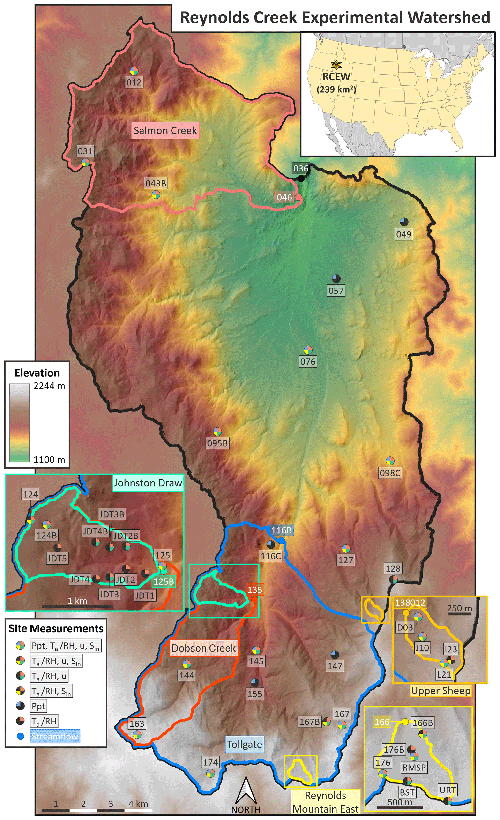
Figure 1 Map of Reynolds Creek Experimental Watershed overlaid on a 10 m digital elevation model with site locations of the meteorological measurements used to produce this dataset. Hourly site measurements include precipitation mass (Ppt), air temperature (T_a), relative humidity (RH), wind speed and direction (u), and incoming shortwave radiation (S_in). Also, the six primary sub-watersheds are delineated by their outlet weir locations where streamflow (Q) is measured. Weir sites are denoted by the solid single-color circles corresponding to the basin boundary colors.

3 Dataset description

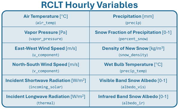
The gridded dataset, called the Reynolds Creek Long-Term (RCLT) dataset, was derived using the dense RCEW station network (one station per 6 km²) maintained by the USDA-ARS-NWRC. Dataset variables include air temperature, vapor pressure, precipitation mass, wet bulb temperature-derived precipitation phase, density of new fallen snow, U- and V-components of wind, incoming shortwave and longwave radiation, and modeled visible and infrared spectral albedo for snow-covered surfaces (Fig. 2). The temporal record spans 40 water years from 1 October 1983 to 30 September 2023 (a water year beginning on 1 October of the previous year and ending on 30 September of the current year).

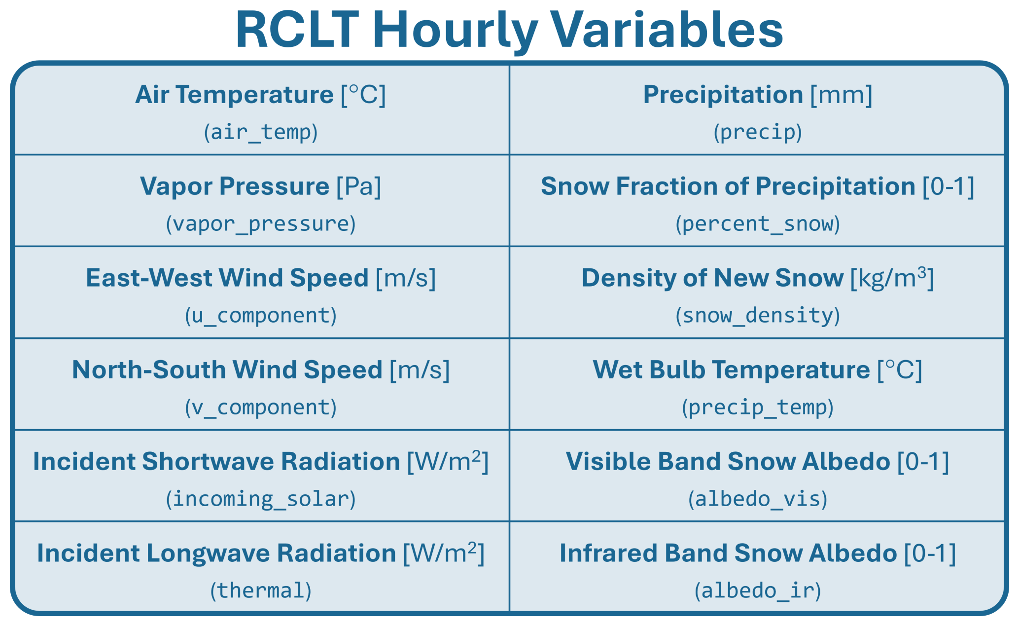
Figure 2 The 12 meteorological variables and their units produced for the high-resolution Reynolds Creek Long-Term (RCLT) dataset. Variable filenames in the Zarr dataset are listed in parentheses.

4 Instrumentation and variable distribution

The Spatial Modeling for Resources Framework (SMRF v0.11.7) (Havens et al., 2017) was employed to distribute each of the 12 land-surface meteorological variables to a 10 m regular grid. Each forcing variable has either been empirically derived or directly interpolated from hourly station measurements across the catchment domain. Owing to the considerable length of time encompassed by the dataset, many different sensors have been deployed in the watershed over the 40-year data record with differing levels of accuracy, which are not reported here but are available upon request. Invalid data were preliminarily removed for all measured variables besides precipitation (which necessitated a unique approach detailed in Sect. 4.6), and temporal interpolation was performed for data gaps of two hours or less. Gaps lasting longer than two hours were left empty with the foreknowledge that spatial interpolation from nearby sites in the high-density network would act as surrogate data for those time steps. It is worth noting that the NWRC has always employed a full-time staff of technicians tasked with the calibration and servicing of each sensor deployed in the RCEW. The gridded interpolation methods for all 12 modeled variables from the six measured variables are described in Hedrick et al. (2018) and further elaborated upon in the following subsections.

4.1 Air temperature

Hourly measurements of air temperature (T_a) were made at 35 individual sites over the 40-year period (Fig. 1), with the number of sites significantly increasing after water year 2000 (Fig. 3). Measurements are currently made using various incarnations of the widely used Vaisala HMP series of temperature and humidity sensors with ventilated radiation shields.

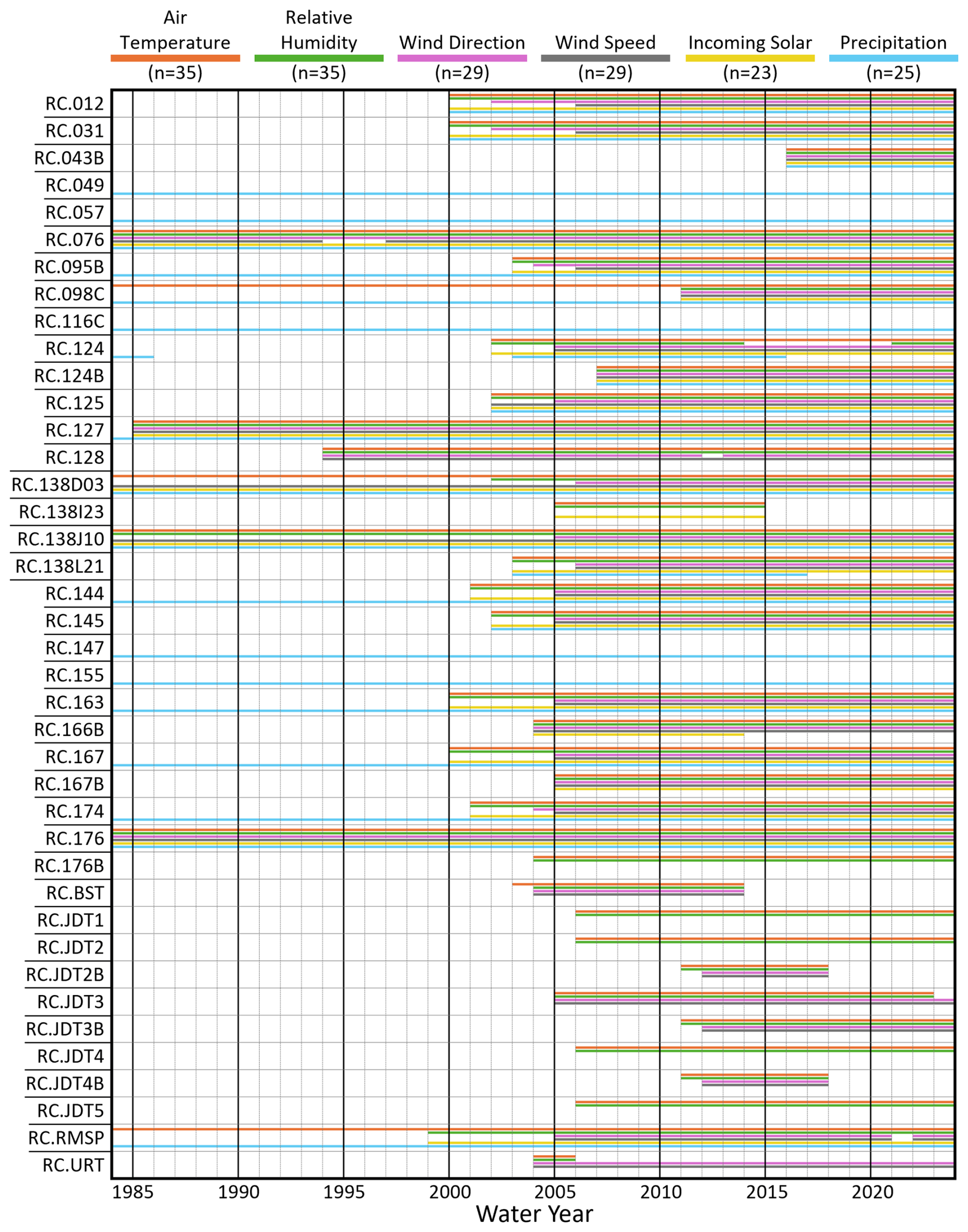
Figure 3 Annual water year measurement record used in SMRF gridded interpolation from the 40 individual sites within RCEW from 1 October 1983 to 30 September 2023. The horizontal bars for each variable indicate station observation data present for over half of a water year, however smaller data gaps are not shown. Some sites measure all six variables required by SMRF to produce the 12 gridded hydrometeorological forcing variables, though many are instrumented to measure fewer variables. For example, five stations solely measure precipitation (RC.049, RC.057, RC.116C, RC.147, and RC.155).

A modified inverse distance weighting (IDW) approach was used to distribute T_a across the 10 m grid. In this process, the elevational trend is calculated at each time step, constrained to be negative due to the general relationship between elevation and T_a, then subtracted from the station measurements to produce a temperature residual. These residuals are distributed using standard IDW and added to each grid cell's position on the elevation gradient slope line. This approach for distributing T_a improves station representativeness for areas with complex mountain topography (Havens et al., 2017). Between 1984 and 2023, the mean annual distributed air temperature across the entire RCEW was 8.4  °C and the all-time maximum and minimum hourly temperatures were 42.4 and −31.5 °C, respectively.

4.2 Vapor pressure

Gridded actual vapor pressure (e_a) values were interpolated from measurements of relative humidity (RH) at the same 35 sites as T_a over the 40-year data record, using the same Vaisala HMP instruments referred to in Sect. 4.1. The empirical Tetens equation was used for deriving e_a from RH and T_a (in degrees Celsius) when temperatures are above freezing:

$$\begin{array}{}\text{(1)}& e_{\mathrm{a}}=\mathrm{RH}\cdot \mathrm{0.6108}\cdot e^{\left(\frac{\mathrm{17.3}\times T_{\mathrm{a}}}{\mathrm{237.3}+T_{\mathrm{a}}}\right)},\end{array}$$

while the Magnus–Tetens equation is used when temperatures are below freezing and the ground surface is assumed to be ice:

$$\begin{array}{}\text{(2)}& e_{\mathrm{a}}=\mathrm{RH}\cdot \mathrm{0.6108}\cdot e^{\left(\frac{\mathrm{21.9}\times T_{\mathrm{a}}}{\mathrm{265.5}+T_{\mathrm{a}}}\right)}.\end{array}$$

Station-derived e_a was then distributed to the 10 m grid using the same modified IDW detrending approach described in Sect. 4.1. Dew point temperature was also calculated for the wet bulb temperature calculation (Sect. 4.6.2 below) but was not stored in the RCLT dataset because it can be calculated from the vapor pressure and air temperature using the existing empirical relationships (e.g., the Clausius–Clapeyron equation). Over the dataset record, the mean distributed e_a across the RCEW was 584 Pa, with a maximum value of 2551 Pa during an intense summer thunderstorm and a threshold minimum of 20 Pa that only occurred during a handful of very cold and dry periods.

4.3 Wind

Hourly average wind speed (u_s) and hourly resultant-mean-wind direction (u_dir) were measured at a total of 29 sites over the data record, though only three sites were available prior to 1994 and four sites prior to 2002 (Fig. 3). The sparseness of wind measurements through the early years of this dataset is likely a source of uncertainty in the distributed wind grids for that period, though we should note that the pre-2002 measurements captured the full elevation gradient in RCEW at low (RC.076), mid (RC.127), and high elevation sites (RC.176) (Fig. 1). Minimum wind speeds were set to a lower threshold of 0.447 m s⁻¹ (1 mph) to match the lower accuracy reported by most cup anemometer manufacturers. Similarly, maximum wind speeds were capped at 35 m s⁻¹ to avoid numerical instability issues when calculating turbulent heat fluxes in physically based energy balance models.

Station measurements of wind were distributed to the 10 m grid using the maximum upwind slope (maxus) terrain parameter described in Winstral et al. (2002, 2009). In short, the underlying digital elevation model (DEM) was used to calculate a maxus value (in degrees) over a user-defined upwind distance (here 300 met) for all possible upwind directions (0 to 360°) in 5° increments. The resulting 72 layers of maxus grids were stored in a lookup library. Then, for each station, the measured wind speed was adjusted to simulate what the wind speed would have been on a flat surface (“flatwind”) using the maxus value for the measured wind direction at the site. Once the adjusted “flatwind” speeds and wind direction components had been distributed across the entire grid using standard IDW, the distributed wind directions were used to find the maxus value for each grid cell, and the distributed “flatwind” speeds were converted back to actual wind speeds.

For the gridded dataset, wind speed and direction were converted into U- and V-components to match the conventions of NWP models such as the WRF and HRRR models. The U-component represents the East-West wind speed, with positive values indicating wind out of the west, while the V-component represents the North–South wind speed, with positive values indicating wind out of the south. Over the dataset record, the mean hourly wind speed was 4.1 m s⁻¹ and the mean resultant wind direction was out of the southwest (227).

4.4 Shortwave radiation

Gridded incoming shortwave radiation (S_in) was measured at 23 sites across the RCEW (Fig. 3) but cannot be directly spatially interpolated from measurements due to the complex terrain and the variable vegetation canopy present across the catchment. Rather, a three-step process produced the hourly gridded S_in product.

1. Hourly clear sky atmospheric S_in was modeled following Dozier (1980) and then corrected for surrounding terrain in each 10 m grid cell following Dubayah (1994).

2. Station measurements of S_in were divided by modeled clear sky radiation to derive a cloud factor (C_fac) at each station pixel (C_fac=1 represents cloud-free conditions), which was then distributed using standard IDW across the domain.

3. Canopy-corrected S_in values were estimated using empirical relationships presented by Link and Marks (1999), where direct beam shortwave radiation under canopy (R_b) can be represented by:

   $$\begin{array}{}\text{(3)}& R_{\mathrm{b}}=S_{\mathrm{b},\mathrm{in}}\cdot e^{-\frac{\mathit{\mu }h}{\cos \mathit{\theta }}}.\end{array}$$

In Eq. (2), S_b,in is the above canopy cloud corrected direct beam radiation, μ is a canopy extinction coefficient, h is the height of the canopy, and θ is the solar zenith angle. Diffuse shortwave radiation under canopy (R_d) was computed by adjusting the above canopy cloud corrected diffuse radiation (S_d,in) by the canopy optical transmissivity (τ):

$$\begin{array}{}\text{(4)}& R_{\mathrm{d}}=\mathit{\tau }{S}_{\mathrm{d},\mathrm{in}}.\end{array}$$

The terrain-, cloud-, and canopy-corrected S_in presented in this dataset is the sum of Eqs. (3) and (4).

When a comparison was performed between modeled and measured S_in across the 40-year record, we discovered that the values for τ and μ presented in Link and Marks (1999), which were derived in the Canadian Boreal forests, led to an overestimation of S_in at open sites by up to 40 %, and an underestimation of S_in at forested sites by 30 % or more. Therefore, manual adjustments of τ, μ, and height parameters were performed to produce S_in values that more closely matched the station observations (Fig. 4). Importantly, the scale difference between point measurements of S_in and averaged S_in across a 10 m by 10 m grid cell precludes direct agreement since shortwave radiation at the ground surface varies over very short spatial scales. However, the general trends in modeled S_in magnitude as a function of cloud cover were well represented in the spatial dataset. Over the dataset record, the mean distributed S_in over the RCEW was 204 W m⁻² (including nighttime hours) and the maximum reported value was 1,401 W m⁻². Though this maximum value exceeds average top-of-atmosphere incoming shortwave irradiance (1340 W m⁻²), cloud enhancement (CE) and albedo enhancement (AE) events have been shown to result in pyranometer measurements of this magnitude at snow-dominated sites (Gueymard, 2017).

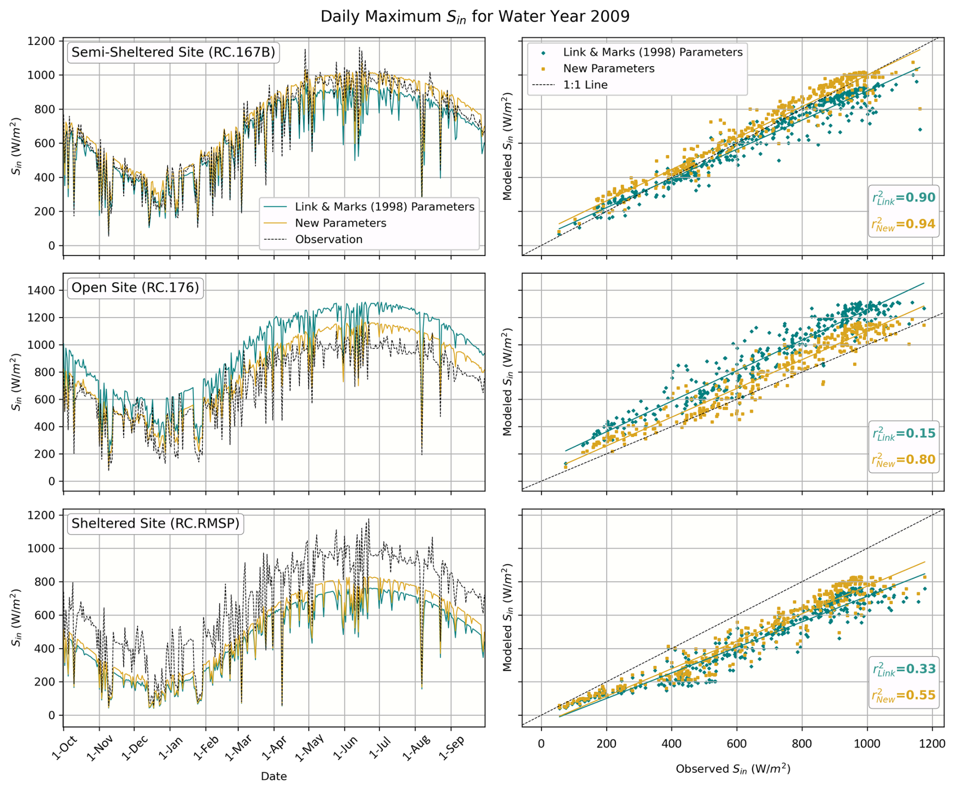
Figure 4 For an example water year (2009), observed versus modeled maximum daily incoming solar radiation (S_in) at three sites with different surrounding canopy coverage. The teal model traces were derived using canopy transmissivity values and extinction coefficients derived by Link and Marks (1999), while the yellow marker traces resulted from new adjusted values to more closely match pyranometer measurements at sites throughout the watershed.

Calculating net shortwave radiation from the RCLT incoming solar product requires an estimate of land surface reflectance, or albedo, and there are many ways to derive an albedo product from both models and remote sensing products. Users of the RCLT dataset are encouraged to use their own methods, but for simplicity we also include here visible and infrared bands of snow albedo for when snow is present. These albedo estimates use a time decay approach to capture albedo change as a function of springtime snow metamorphism, terrain factors, and solar zenith angle (Marshall and Warren, 1987). Importantly, these albedo estimates do not apply for snow-free conditions and would need to be masked for general land surface modeling applications.

4.5 Longwave radiation

Incoming longwave radiation (L_in) was also not directly interpolated from observations since the network lacked upward looking pyrgeometers for measuring thermal radiation during long periods throughout the RCLT time domain. Instead, clear sky L_in was empirically estimated from distributed air temperature and humidity using the methods of Brutsaert (1975), then corrected for surrounding terrain using equations presented in Marks and Dozier (1979). Next, cloud-corrected L_in was computed using the empirical relationship described by Garen and Marks (2005) and the same cloud factor calculated from the incoming shortwave radiation. The final step was an adjustment to the cloud-corrected L_in using vegetation maps derived from the LANDFIRE 2016 dataset (LANDFIRE, 2016) and empirically derived transmissivity (τ) reported by Link and Marks (1999) then modified as described in Sect. 4.4. Over the dataset record, mean L_in across the RCEW was 290 W m⁻², with maximum and minimum hourly values of 600 and 83 W m⁻², respectively.

4.6 Precipitation

To satisfy the standard input requirements of an energy and mass balance snow model, the RCLT dataset contains four distinct variables related to precipitation in the basin. These variables of precipitation mass, temperature of the falling hydrometeor, initial density of newly fallen snow, and the snow proportion of precipitation are described in the following subsections.

4.6.1 Precipitation mass

Despite being the foundation upon which hydrologic models rely, precipitation measurements are often the largest source of predictive hydrologic uncertainty (Bárdossy et al., 2022). Across the wide spectrum of snow-dominated watersheds in the Western US, the majority of in situ measurements are made with weighing buckets fitted with alter shields that reduce wind speeds above the bucket orifice and thus increase the gauge catch efficiency (CE), or the ratio of measured precipitation to a “true” value (Thériault et al., 2021). However, many sites lack co-located wind speed measurements for applying the necessary World Meteorological Organization (WMO) transfer functions for undercatch correction (Kochendorfer et al., 2018), which can lead to low biases in regional and basin estimates of precipitation. Additionally, precipitation exhibits high spatial heterogeneity in complex terrain, which cannot be captured by a single measurement site in a large mountain basin.

To overcome the issue of spatial representativeness, the RCEW measurement network was initially planned to contain one gauge for every square mile with 110 stations in the watershed. By the beginning of this dataset in water year 1984, the number of sites had been reduced to the 25 stations (∼1 measurement per 10 km²) used here to produce the hourly gridded precipitation fields.

To address the undercatch issue, a unique dual-gauge approach (Hamon and Cox, 1972) was used for all sites in the RCEW except for RC.124B. This method requires two co-located Belfort-type weighing buckets with one existing unshielded and the other fitted with a single-alter shield. The combination of the shielded and unshielded measurements allows an empirical extrapolation of more accurate “actual” precipitation data compared with single shielded gauges employing a WMO transfer function (Hanson et al., 2004). Site RC.124B is the only single shielded gauge in the basin and was corrected using the WMO transfer function. Hourly measurements of precipitation mass were distributed across the 10 m grid using a Detrended Kriging interpolation method (Garen et al., 1994), which is identical to the approach by Kormos et al. (2018). Over the dataset record, the mean annual precipitation normalized over the RCEW was 461 mm, with a maximum of 686 mm (water year 1984) and a minimum of 279 mm (water year 1994). However, due to the large elevational gradient in precipitation, the mean for the high elevation Reynolds Mountain East sub-catchment (0.4 km²) was 913 mm while conversely the mean for the low elevation Nancy Gulch sub-catchment (0.3 km²) was only 325 mm.

4.6.2 Precipitation temperature

The precipitation temperature variable is represented by the hourly computed ice or wet bulb temperature calculated with a widely used Newton-Raphson iterative solution to the psychrometric equation (Campbell and Norman, 1998). This approach requires air temperature (Sect. 4.1), dew point temperature (from calculated vapor pressure in Sect. 4.2) and estimated atmospheric pressure from elevation. Previous research has demonstrated that wet bulb temperature is the most suitable precipitation phase partitioning method in a semiarid watershed such as the RCEW (Marks et al., 2013).

4.6.3 Density of new snow

Hourly estimates of new snow density are included in the RCLT dataset for energy and mass balance snow models that may require it. For this long-term application, we computed new snow density from a lookup table based on previous work (pg. 2007, Susong et al., 1999) using the calculated precipitation temperature (see Sect. 4.6.2) and precipitation mass (see Sect. 4.6.1) in each grid cell. These lookup table values are distributed in a stepwise fashion between −5 and +0.5 °C with values ranging between 75 and 250 kg m⁻³, respectively. Snowfall occurring below −5 °C, which rarely occurs in the RCEW, is assigned a new snow density of 75 kg m⁻³.

4.6.4 Snow fraction of precipitation

In addition to new snow density, the lookup table from Susong et al. (1999) was also used to determine the amount of precipitation that fell as snow across the catchment. When time step precipitation temperatures fell between −0.5 and +0.5 °C, the precipitation was defined as mixed phase. The relationship between precipitation phase and wet bulb temperature is linear such that 0C results in a 0.5 snow fraction, −0.5 °C is 100 % snow, and +0.5 °C is 100 % rain.

4.6.5 Example dataset use case

This dataset allows a detailed analysis of the storm-by-storm precipitation amount, spatial extent, and phase over the 40-year record. As an example of the utility of this unique dataset, we examined how the annual average storm-based rain/snow transition elevation (RS_z) has changed over time in the snow-dominated 55 km² Tollgate sub-watershed in the southern portion of the RCEW. We began by designating storm hours as any time steps in which any pixel in the catchment area received above a precipitation threshold of 0.5 mm. Next, storm periods were defined for consecutive hours with a maximum storm hour threshold of 6 h. For each storm hour, the mean elevation of mixed phase precipitation (e.g. grid cells where −0.5 °C < T_wb < 0.5 °C) was computed and mass-weighted by precipitation amount, then the hourly mean elevation was mass-weighted across the storm period. Lastly, those elevations were further mass-weighted by storm total precipitation to arrive at water year and accumulation season mean RS_z (Fig. 5a). The accumulation season was defined as the period from 1 October to peak snow water equivalent (SWE) accumulation at the Reynolds Mountain Snow Pillow site (RC.RMSP). Overall, the snow-dominated portion of the catchment has retreated toward higher elevations. When considering all storms throughout each water year, the RS_z has risen from 1830 m in 1984 to 1991 m in 2023, resulting in a decrease in snow-dominated basin area from 52 % to 24 % (Fig. 5b). For storms during the accumulation season, the RS_z has risen from 1580 to 1708 m between 1984 and 2023, with the snow-dominated basin area decreasing from 91 % to 74 % (Fig. 5c).

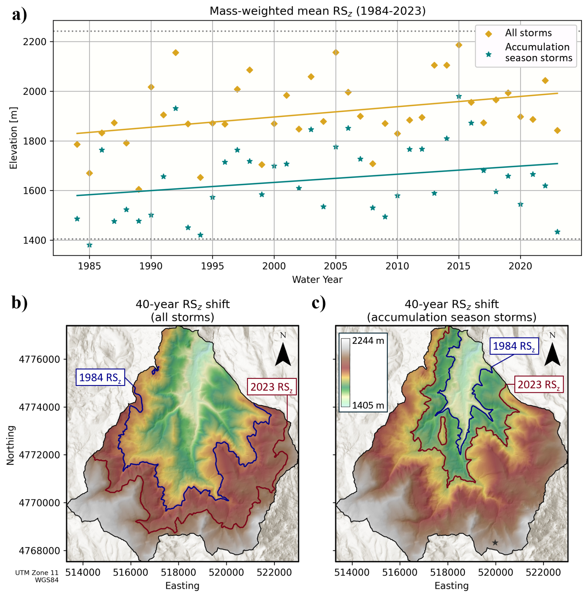
Figure 5 (a) The annual precipitation mass-weighted mean rain/snow transition elevation for water years 1984 to 2023 in the Tollgate sub-watershed for all storms over the course of a full year (orange diamonds and orange line of best fit) and the snow accumulation season from 1 October to peak SWE date (blue stars and blue line of best fit). Horizontal dotted lines represent the upper and lower elevations of the Tollgate sub-watershed. (b) The RS_z in 1984 (blue) and 2023 (red) when considering all storms in each year. (c) Same as (b) but only considering storms occurring from 1 October to the date of peak SWE at the Reynolds Mountain snow pillow (denoted by the black star).

5 Data availability

The gridded dataset in its published form is at hourly temporal and 10 m spatial resolution, which was determined to be optimal for users requiring high resolution forcing data while also being suitable for disk storage. NetCDF files, though standard format for meteorological data, can become unwieldy when file sizes become too large, which is mitigated by the cloud-optimized Zarr format (Miles et al., 2023) that can be read by programming libraries in python, R, C$++$, and Java. Nevertheless, users that desire a coarser spatiotemporal RCLT dataset have two options for decreasing resolution. The simplest approach would be to read the provided high resolution files, resample to desired resolution using mean or sum values across space and time, and save to a new NetCDF file. A slightly more accurate approach would be to install SMRF locally, create a model setup file at the desired spatial resolution, edit the configuration files to define the coarser temporal resolution, and run the distribution code. However, this approach will require detailed knowledge of the software and is not recommended for most users. An example SMRF configuration file for a single water year and all station data CSV files organised by water year are provided in the Supplementary Materials.

Accessing temporal and spatial slices of this 13 TB dataset is straightforward as it is stored as cloud-optimized Zarr-formatted files and hosted by the open-access Ag Data Commons data repository (https://doi.org/10.15482/USDA.ADC/30199954, Hedrick et al., 2025) maintained by the USDA National Agricultural Library (https://agdatacommons.nal.usda.gov, last access: 22 July 2026). Users may download either the entire 40-year record or by individual water year (∼325 GB yr⁻¹) through the linked Globus web interface. It is also recommended that users work with the dataset on a High-Performance Computing (HPC) or Cloud environment with parallel processing capabilities. An example jupyter notebook script for loading the Zarr-formatted data using the python Xarray package is provided in the repository. The coordinates are stored as projected coordinates in UTM Zone 11 using the WGS84 geodetic reference system. At 10 m spatial resolution, the model domain shape is 3010 (north–south) by 1602 (east–west) pixels. The time domain is 350 640 total time steps, resulting in 1.7 trillion total stored values per variable, or 20.3 trillion stored values across the entire dataset. A tagged release for the SMRF source code used to create this dataset is available at https://github.com/iSnobal/smrf/releases/tag/20250926 (last access: 22 July 2026; https://doi.org/10.5281/zenodo.21514687, Meyer et al., 2025).

6 Summary

The RCLT dataset comprises all meteorological forcing variables required to simulate the accumulation and melt of the seasonal snow cover using a mass and energy balance snow model as well as the fundamental land surface variables estimated by Numerical Weather Prediction models and historical atmospheric reanalysis products. The RCLT provides unique opportunities for comparison of various physically based models, evaluation of long-term atmospheric reanalysis datasets, and new studies on agroecosystem response to differing weather patterns. By publicly sharing this dataset in a cloud optimized format, we support modern software workflows, analysis, and open science best practices to support the broader science community. Maintaining and regular releasing long-term in situ network data is an important contribution to better understand and predict future water availability in snow-dominated watersheds.