EARLS: a runoff reconstruction dataset for Europe

Data drives our understanding of hydrological processes, supports model development, and enables anticipatory water management. This contribution introduces EARLS: European Aggregated Reconstructions for Large-sample Studies. EARLS offers daily streamflow reconstructions for more than 10 000 basins in Europe including uncertainty estimates, covering the period from 1953 to 2023. The reconstruction is derived from a single Long Short-Term Memory (LSTM) based rainfall–runoff model trained on more than 5000 basins. LSTMs represent the state of the art in rainfall–runoff modeling and are well suited to provide predictions in ungauged basins. We evaluate the quality of the reconstruction through quantitative evaluation on two held-out sets of basins and by conducting a qualitative assessment that compares EARLS-based peak flows and flood timing to previous large-scale hydrological studies. EARLS represents a new generation of datasets that harness the capabilities of Deep Learning to obtain accurate and high-resolution data. EARLS is available at https://doi.org/10.5281/zenodo.13864842 (Klotz et al., 2026b).

1 Introduction

Data availability is central to hydrological science. It is the basis for advancing our understanding of hydrological processes, building prediction models, and anticipatory water management. However, in many regions and periods, observations are scarce. Practitioners often rely on hydrological model predictions to compensate for these deficiencies (e.g., Beck et al., 2015; Do et al., 2018; Ghiggi et al., 2019; O and Orth, 2021). The resulting dataset are referred to as reconstructions. More generally, we can think of reconstructed data as datasets that are generated from observational records with the aid of models to address gaps in the data. There exist many challenges associated with making reconstructions. In particular, the non-linearity between drivers and the unique characteristics of each basin make it difficult to use process-based hydrological models for high-quality reconstructions (e.g., Addor et al., 2018). Here, purely data-driven approaches provide a great opportunity. Current approaches based on Machine Learning (ML) are able to simulate a diverse range of rainfall–runoff responses when trained using data from multiple basins (Kratzert et al., 2019b, 2024). They are able supply high-quality predictions (e.g., Kratzert et al., 2019b; Mai et al., 2022; Jiang et al., 2022, 2024) and are often suitable for simulating even in ungauged basins (Kratzert et al., 2019a; Nevo et al., 2022; Nearing et al., 2024). These characteristics render data-driven approaches an exceptional but currently underused tool for large-scale hydrological analyses.

Data availability also plays a particularly important role in Large Sample Hydrology (LSH). LSH concentrates on multiple basins, as opposed to conducting detailed studies in individual regions. A central question in LSH is how we can transfer knowledge about runoff responses between different basins, given their hydrological similarities (e.g., Hrachowitz et al., 2013; Peters-Lidard et al., 2017). Large-scale datasets allow us to identify patterns and formulate conclusions about hydrological processes across diverse regions. Recent advancements in LSH have led to the development of several large-scale hydrological databases, compiling streamflow records from multiple locations. Notable global databases are: (1) The Global Streamflow Indices and Metadata Archive (GSIM; Do et al., 2018; Gudmundsson et al., 2018), which contains monthly, seasonal and yearly indices for over 35 000 locations; (2) The Global Runoff Data Center database (GRDC; Bundesanstalt für Gewässerkunde (BfG), 2023), which provides discharge estimates for over 10 000 locations; and (3) The Caravan project (Kratzert et al., 2023; Färber et al., 2023), which incorporates already open-source published streamflow data from various countries.

The requirement to drive rainfall–runoff models with meteorological forcings led to the development of integrated datasets that include meteorological time series such as precipitation and temperature. To our knowledge, the Model Parameter Estimation Experiment (MOPEX Duan et al., 2006) provided the first openly available large sample dataset of this kind. It contains 431 basins within the United States. Some of the most important contributions in popularizing large-scale datasets after MOPEX stem from the basin Attributes and MEteorology for Large-sample Studies (CAMELS) initiatives (Addor et al., 2017; Alvarez-Garreton et al., 2018; Coxon et al., 2020; Chagas et al., 2020; Fowler et al., 2021; Höge et al., 2023; Loritz et al., 2024), and other derivations such as LamaH (Klingler et al., 2021; Helgason and Nijssen, 2024) and CABra (Almagro et al., 2021). Each CAMELS dataset is tailored to a specific region, but at its core follows the same logic–connecting meteorological variables and static basin attributes with streamflow data. The Caravan project (Kratzert et al., 2023) incorporates already open-source published streamflow data from various CAMELS countries – and with its recent extension also contains the sharable GRDC data (Färber et al., 2023). In this study, we however use EStreams (do Nascimento et al., 2024) as our “raw material” for model building. EStreams also constitutes an integrated dataset, but goes into a different direction: It provides basic data for setting up hydrological models, but also a catalog streamflow data from national data providers. Unlike the CAMELS and Caravan datasets, it focuses only on the European scale. It also offers higher spatial resolution, and is designed to be continuously updated, providing the latest records in both time and space.

Despite these numerous developments in building large-scale databases for hydrology, important sampling gaps exist. This holds in particular with respect to high-quality runoff observations. This limits the usability of said databases for certain scientific applications and decision-making processes at a pan-European level. To address these limitations, here we present a data-driven daily runoff reconstruction product for natural streamflow. We name it EARLS: European aggregated reconstruction for large-sample studies. Our main goal for EARLS is to provide data-driven streamflow reconstructions that enable the analysis of hydrological processes in the style of Blöschl et al. (2017). The reconstructions represent daily simulations of natural streamflow, are provided in mm, and cover the period from 1953 to 2020.

One can view EARLS as part of a new generation of datasets that leverage ML to achieve highly accurate predictions (e.g., O and Orth, 2021; O et al., 2022; Nasreen et al., 2022; Kraft et al., 2025). We employ a rainfall–runoff model based on Long Short-Term Memory (LSTM; Hochreiter and Schmidhuber, 1997) to create these reconstructions. Recent studies have demonstrated the accuracy of this approach in various contexts (e.g, Kratzert et al., 2019b, a; Mai et al., 2022; Nearing et al., 2024). The model incorporates static attributes that describe basin properties (say, average elevation) and a series of meteorological forcings (say, daily precipitation) to simulate streamflow for a given basin, following the approach introduced by Kratzert et al. (2019b) and Klotz et al. (2022). We evaluate the resulting simulations in terms of predictive performance for ungauged basins. Like EStreams, EARLS focuses on Europe. In particular, we use a subset of the EStreams basins with CAMELS attributes for training our model (see Sect. 2.1), aiming to provide spatially extensive long-term streamflow reconstructions with uncertainty estimates, including for ungauged basins across Europe.

2 Method

EARLS provides streamflow reconstructions for 17 043 European basins. The data are in daily resolution, comprise uncertainty estimates, and span for each basin from 1 January 1953 to 30 June 2023. The time period is constrained by the meteorological forcing used (see below). We plan to extend it later as the meteorological dataset gets updated. Gaps in the reconstructions only occur when the dynamic inputs are erroneous – which can happen if the meteorological forcing have gaps at different timesteps. EARLS contains 14 161 basins without data gaps, 2655 with gaps of variable lengths, and we were not able to produce a simulation for 227 basins (these are not part of the 2655 basins wit gaps). For these basins there is so much missing data in the inputs that our modelling approach is not able to make simulations at all. We also keep these in EARLS since the meteorological forcing is regularly revised and we plan to update on a regular basis (Sect. 4). Since it is not appropriate for royalty to be alone, we plan to produce EARLS versions with less and less gaps in the future, and eventually even start sister projects with different focal points. The basins for model training are from EStreams (Sect. 2.2.1). However, we also derive a set of virtual ungauged basins to provide continuous spatial coverage (Sect. 2.2.1). The model is lumped (which necessitates an aggregation of the inputs at the basin level) and provides not only point estimates but also uncertainty estimates in the form of a distribution prediction. Section 2.2 provides an overview of the modeling setup.

2.1 Training and evaluation data

We spatially aggregate dynamic inputs (i.e., meteorological forcings) and static inputs (i.e., basin-specific static attributes) for each basin. The basin shapes are either derived from EStreams (do Nascimento et al., 2024) or HydroATLAS (Linke et al., 2019). When both shapes are available we use both for the training. All streamflow data is in millimeters per day (mm d⁻¹). We use 4 dynamic inputs (i.e., precipitation, minimum, maximum, and mean temperature) that we aggregate basin wise from version 28 of E-OBS dataset (Klein Tank et al., 2002; Haylock et al., 2008). This means that we do not use all available dynamic inputs, i.e., we do not leverage all information that we could. The EARLS LSTM will not provide the best possible predictions (indeed, albeit we do not show the results here, we did make some experiments with more inputs and did obtain better results; see also: Kratzert et al., 2021). However, we believe this disadvantage is offset by the increase of flexibility in use of the model. E-OBS is a daily-resolution gridded dataset covering the European region (25–71.5° N × 25° W–45° E). This defines the extent of EARLS in both space and time. E-OBS interpolates station data from European National Meteorological Services and other providers, spanning 1 January 1950 to present (in EARLS the modelling period starts, however, in 1953, since we use the first three years as buffer time). It comprises time series of meteorological variables such as daily mean, maximum, and minimum temperature, daily total precipitation and mean sea level pressure. For the static inputs, we use 13 attributes that we aggregate from HydroATLAS (following the convention from Caravan; Kratzert et al., 2023): basin area, the average elevation, the average slopes, the average stream gradient, the average long-term air temperature, the minimum long-term air temperature, the maximum long-term air temperature, a global aridity index (Zomer et al., 2022), a global climate moisture index (Hijmans et al., 2005), the average fraction of sand the average fraction of clay, the average fraction of silt, and the average organic carbon content. We chose this subset for the sake of simplicity, but, in general, different inputs and combinations therefore are thinkable to create new models and datasets.

The streamflow training data originate from national and regional hydrometric through the EStreams catalog. The streamflow data are generally accessible through the respective agencies; however, they are distributed under heterogeneous licensing conditions (as Do et al. (2018) mention, availability of does not necessarily imply permission for third-party redistribution). Consequently, and in accordance with the data governance approach adopted for EStreams, the raw daily streamflow observations that we use for model training are not redistributed as part of the EARLS dataset. Instead, the full documentation of the original data providers and references to the corresponding sources are available in the Supplement and the data publication (Klotz et al., 2026b). This allows users to obtain the records directly from the responsible agencies under their respective licensing frameworks.

2.1.1 Preprocessing

To get streamflow observation we alleviate EStreams (do Nascimento et al., 2024). EStreams contains hydro-climatic variables and landscape descriptors, and references to openly available streamflow records for 17 130 European basins. It includes basin delineations, hydro-climatic signatures, and landscape attributes (topography, soils, geology, vegetation, and land cover), and gives the necessary information to access daily streamflow data from the data providers, which we cannot redistribute (see above). The data quality of EStreams basin does, however, vary considerably. We filter out gauged basins according to the following criteria:

1. Each basin needs to have high-quality delineations (see Table 3 in do Nascimento et al., 2024).

2. To minimize aggregation errors in the basin mean attributes and simultaneously reduce the effects of channel routing, we only include basins equal or larger than 50 km² and smaller than 100 000 km².

3. We require each basin to have at least 30 years of, not necessarily consecutive, daily streamflow observations.

4. We exclude basins which, based on the attributes derived in EStreams, include more than four dams or reservoirs within the basin boundary.

5. We require the presence of meteorological time-series from E-OBS for the basins.

6. We exclude basins where hydrological signatures indicate potential data problems, based on the following criteria:

   • a.

     The long-term average streamflow needs to be below 10 mm d⁻¹.

   • b.

     The long-term runoff ratio (as defined in Sawicz et al., 2011) cannot be larger than 1.

After applying these constraints to the EStreams catalog, we are left with 5786 basins with streamflow observations (blue circles in Fig. 1; see also Appendix A). We further partitioned these into 4789 training basins, 500 chosen basins for validation, and 500 for testing. That is, we do not apply any time split for the training and evaluation of the EARLS LSTM. In other words, validation is carried out in space, but not in time.

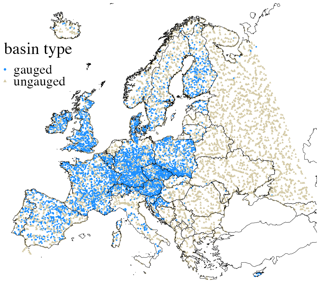
Figure 1 Spatial distribution of the gauged (blue circles) and ungauged basins (grey triangles).

Our preprocessing is not perfect. Specifically, many of the low basins (a) are influenced by human activities, such as the presence of dams and reservoirs (Portugal and Spain); (b) exhibit extensive canal systems and numerous lakes (Denmark, Sweden, and Norway); (c) contain karstic geology (Central Europe); or (d) are situated regions where the meteorological forcing data are scarce (Iberian Peninsula and southern Italy; see Do et al., 2018). In our data preprocessing we filter out basins that exhibit a high degree of human influence (Sect. 2.2.1). In Spain and Portugal, anthropization is primarily caused by numerous dams constructed for water supply. The identification of such structures at such a large-scale is challenging (Senent-Aparicio et al., 2024). Hence, EStreams may not correctly capture the total number of dams and reservoirs in many regions because of the used data sources (as discussed in Salwey et al., 2024). Furthermore, the high number of natural lakes and the presence of canalization systems may also negatively influence the model's performance in these areas. The same applies for the presence of karstic systems, which poses a challenge for closing the water balance in some basins. EStreams made significant efforts to label such basins do Nascimento et al. (2024). However, despite the efforts we were not able to produce ex-ante labels for said basins or create an adequate criterion to filter them out (Sect. 2.2.1). This affects both, model training and evaluation, since some signals are not learnable in the first place.

2.2 Rainfall–runoff model

Our LSTM-based rainfall–runoff model uses dynamic and static inputs to estimate streamflow. Since the LSTM is a deep learning architecture we will use concepts and language from machine learning to describe how we set it up. For example, for the model selection we will use a triple split (training, validation, and test set) and we will refer to the selection procedure as training (and not, say, as model calibration as is usual in hydrology). To provide uncertainty estimates, we adapt a simplified version of the approach from Klotz et al. (2022). In short, instead of estimating the streamflow directly, the LSTM outputs the three parameters of an asymmetric Laplacian distribution (a double exponential with a parameter) – and is trained using maximum likelihood (Fig. 2). Appendix B provides a short overview of our approach. For a more detailed and general exposition we refer to Klotz et al. (2022). From here on out we refer to this model as the EARLS LSTM. The next two sections describe how we set up the training and evaluation of the EARLS LSTM. Further technical details are available in Appendix A.

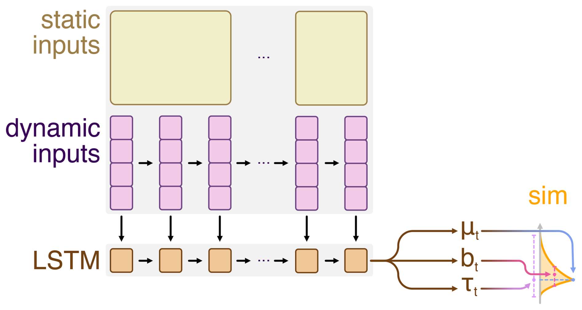
Figure 2 High-level model conceptualization. For each time step t The LSTM outputs the location parameters μ_t, the scale parameter b_t, and the asymmetry parameter τ_t to parameterize an asymmetric Laplace distribution for each predicted timestep. For the use and definition of the static and dynamic inputs we refer to Sect. 2.2.1.

2.2.1 Streamflow reconstructions

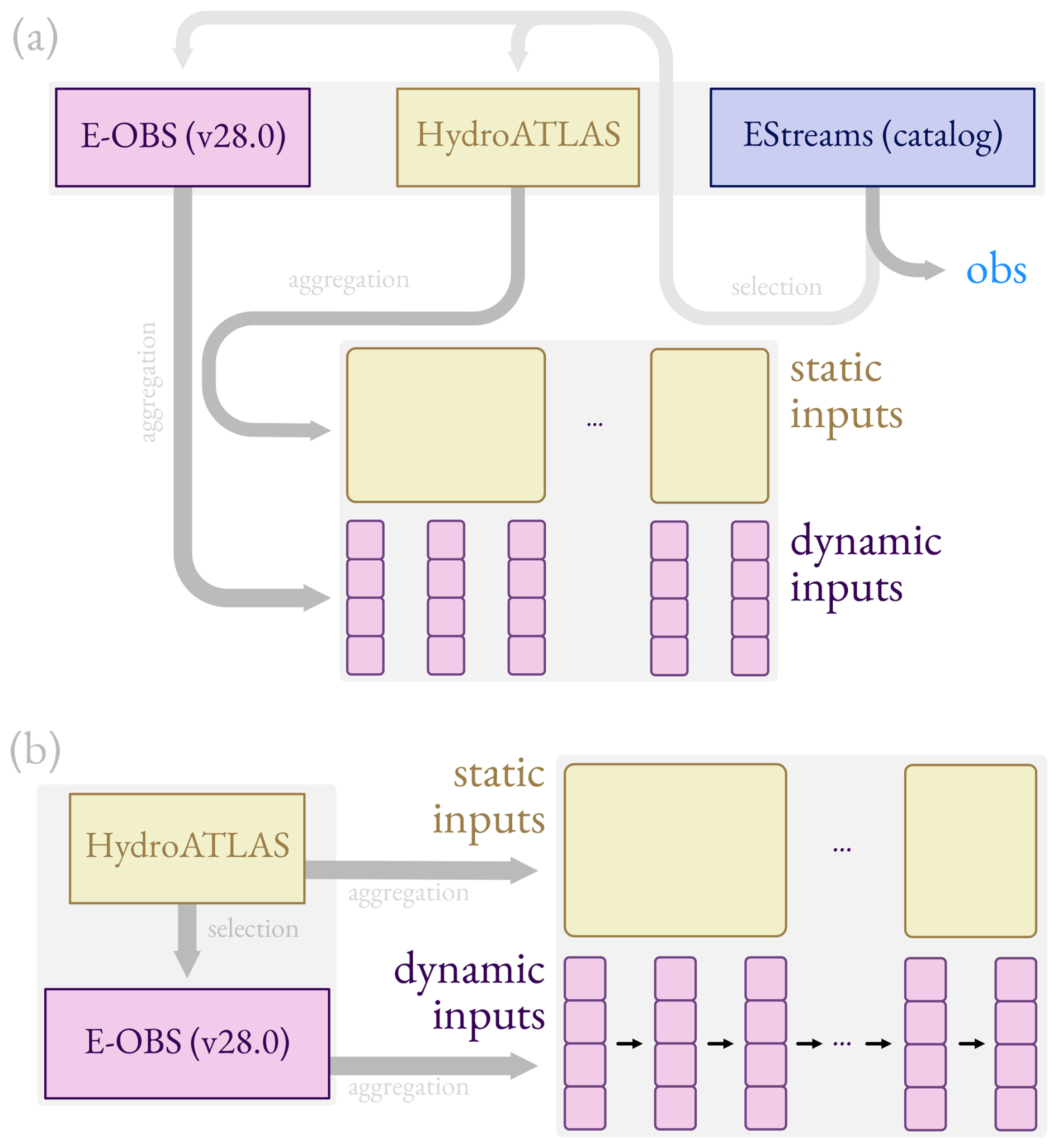
Figure 3 Overview of the modeling setup for the (a) gauged and (b) ungauged basins. The yellow boxes indicate that we concatenate the same static input for each timestep. The static attributes are just different from basin to basin. In contrast, the dynamic input vary for each timestep (and basin).

Our model setup deviates slightly between gauged and ungauged basins (Fig. 1), since for the latter no observations are available (Fig. 3). Specifically, we use the gauged basins for training and evaluating the EARLS LSTM (Fig. 3a). For each gauged basin we use the observations from the EStreams catalog (Sect. 2.1.1), the static inputs from HydroATLAS, and the dynamic inputs from E-OBS. The ungauged basins (Fig. 3b) are the basins without corresponding observations. They add a set of virtual basins as additional support basins for EARLS. The goal here is to achieve dense coverage across Europe (gray basins in Fig. 1). We delineate the ungauged basins from the union of all upstream level 12 polygons of the level 12 layer of HydroATLAS. Like in the gauged case, the static and dynamic inputs are derived from HydroATLAS and E-OBS, respectively. The resulting “simulation layer” consists of 11 277 basins (some overlapping with the gauged basins), which yields a total of 17 043 EARLS basins when combined with the gauged basins that we use for training.

2.3 Evaluation

We corroborate the data quality of EARLS by evaluating the model performance on a large set random test basins. On top of that, we provide extensive appendices that examine the data properties with a mix of quantitative and qualitative measures (Appendix C: We examine whether model performance is related to static or dynamic basin characteristics (Appendix C1), perform a comparative analysis with a process based model on the basis of 161 separately chosen basins (Appendix C2), and conduct a qualitative assessment against published literature results (Appendix C3).

For the model evaluation we report the performances for the training, validation and test set (for a technical definition we refer to Appendix A1). It normally does not make sense to report training and validation performances in a ML context, since one is generally interested in generalization – and performance measures are biased for the training and validation sets. However, since we also publish simulations for these basins we argue that it is informative for users to also report the respective performances. Specifically, we report Nash–Sutcliffe efficiency (NSE) for each basin and over the time horizon of a given portion. For a given basin it is defined as:

$$\begin{array}{}\text{(1)}& \text{NSE}=\mathrm{1}-{\displaystyle \frac{{\sum }_{t=\mathrm{1}}^T(o_t-s_t{)}^{\mathrm{2}}}{{\sum }_{t=\mathrm{1}}^T(o_t-\overline{o}{)}^{\mathrm{2}}}},\end{array}$$

where $t=\mathrm{1},\mathrm{2},\mathrm{\dots },T$ is the time index for the given basin and time horizon, o the observations, s the simulations, and $\overline{o}=\mathrm{1}/T{\sum }_{t=\mathrm{1}}^T{o}_t$ the sample mean of the evaluated data. Appendix D also reports the model performance on the test set with regard to other metrics.

3 Evaluation results and discussion

In the following, we show the results of our model evaluation. To assess the model performance we compute the NSE for 500 test basins over the full range of the EARLS time horizon (i.e., 1953–2023). The EARLS LSTM achieves a median NSE of 0.66 for the 500 test basins. We view this as a good result, given our splitting strategy, which leads to potentially difficult to predict ungauged basins for the evaluation (Sect. 2.1 and Appendix A1), and the utilization of only a single dynamic input product (as, for example, opposed to Kratzert et al., 2021, who examine the use of multiple forcings). On top of that, our pre-filtering strategy is rather coarse (see Appendix A), hence many (ungauged) basins remain in the dataset that can be difficult to handle (e.g., Karst-affected catchments). Still 10 % of the basins exhibit NSE values that are lower than 0.0 (Fig. 4a).

To give readers a rough comparison: These results are similar to the ones in Kratzert et al. (2019a), who report that 8 % of the basins exhibit negative NSE values. The highest basin has an NSE of 0.93 and the lowest of −25.42. These values are not randomly distributed in space (Fig. 4b). Appendix D provides empirical cumulative distribution functions for other metrics.

We posit that most low accuracy values can be attributed to data quality issues rather than to shortcomings in the LSTM (Sect. 2.1.1). On top of that it is worth to remember that that there is evidence that the NSE can be rather erratic in arid climatic regimes (e.g., Duc and Sawada, 2023; Klotz et al., 2024; Knoben, 2024).

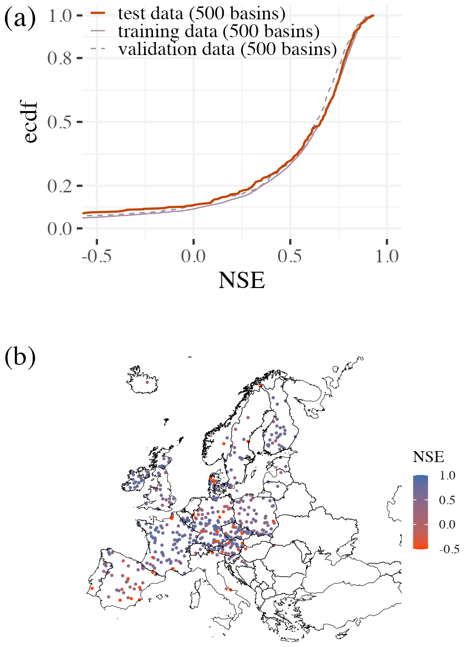
Figure 4 Performance evaluation. For both plots we clip the negative values of Nash–Sutcliffe efficiency (NSE) at −0.5 to focus on the important part of the performance distribution. (a) Empirical cumulative density function. Each point on the line represents the model performance for one of the 500 test basins. The red-solid line shows the performance for the test data. The dashed lines show the performance for the training and validation data. (b) The correspondend spatial distribution of the respective NSE values.

3.1 Limitations

Our results suggest that EARLS as a dataset is well suited for large-sample hydrological studies in Europe. However, there exist several important limits to EARLS: The simulation quality is restricted by (a) the streamflow observation quality, (b) the input quality, and (c) the capabilities of the EARLS LSTM. The quality of streamflow and input data varies in space (e.g., different measurement standards across countries) and time (e.g., improvements in measurement technique over time). As a matter of fact, some of the observations are highly atypical. It would not be surprising if they cannot be modeled with the available information. The same kind of reasoning applies to the forcings. For example, E-OBS is more accurate in high station-density regions like Germany and Austria, and less so in lower density areas like Spain, Portugal, or Eastern Europe (see do Nascimento et al., 2024). These results suggests the existence of non-trivial distribution shifts in the reconstructions. From a machine learning perspective distribution shifts are challenging to model well. Lastly, with regard to (c), a machine learning model – such as the EARLS LSTM – by design, can only capture the signal that is in the data. We chose an LSTM-based approach since it represents the best simulations in gauged and ungauged settings (Kratzert et al., 2019b, a; Mai et al., 2022; Nearing et al., 2024). Nonetheless, we kept the setup simple for ease of use. For instance, we use a limited set of dynamic inputs that are available in many observation-based datasets and use a simple single Laplacian distribution in the output and a single meteorological product for the dynamic inputs. We did not conduct extensive intercomparisons and expect better results with more complex setups. In that case, the current EARLS version will serve as a (strong) baseline.

Further, EARLS incorporates distributional prediction for each time step by providing the conditional parameters of an asymmetric Laplace distribution (Sect. 2.2). This does not represent the full uncertainty of the prediction. On top of that, the conditional distribution assumes no knowledge of the streamflow. Thus, if we naively take samples at a given time step, then this does not account for the autocorrelative nature of the streamflow.

4 Data and code availability

The project homepage for EARLS is https://earls-dataset.github.io/ (last access: 13 July 2026). We envision the page as a living document for future news and updates. The EARLS data is available at https://doi.org/10.5281/zenodo.13864842 (Klotz et al., 2026a). It includes streamflow reconstructions for 17 043 European basins. We build the dataset with extensibility in mind. The idea here is that the current structure becomes a blueprint for potential future expansions. Specifically, the data of EARLS is organized as follows:

• The “coordinates.csv” file contains basin outlet information with 5 columns: basin id (idx), type, and estimated latitude (lat) and longitude (lon) of the outlet, and the distance to the nearest gauged station. The type indicates whether the streamflow information of a given basin was used for training. Together with the information of nearest gauging station it can be used by analysts to demarcate whether a reconstruction is well supported by the training data (see Appendix F).

• The “license.md” file contains information about the licensing.

• The “shapefile” folder includes a shapefile with all basin boundaries.

• The “reconstructions” folder contains CSV files. In general, each file is named after the basin id and has at least the columns for date (date) and simulation (sim). The simulations are given in mm d⁻¹ and we use the location parameter of our conditional distribution estimate. To provide a probability density estimate for each reconstruction timestep in EARLS we added two additional columns (namely: tau and b). Together with the location parameter (saved as sim) these fully define an asymmetric Laplacian. Hence EARLS comprises uncertainty estimates for each time step (Sect. 2.2).

• The “model-card” folder contains 3 files: “model-card.html”, and “earls-crest.png”. The html document includes the png as logo and renders a model card. A model card is a short summary of the model genesis, designed to increase transparency by communicating information about trained models to broad audiences (Mitchell et al., 2019). We include all three files in the dataset so that future extensions can adapt them with maximal ease. We will also host the markdown files on the main home so that the permanent identifier within the model card can be used to access the data from there.

• Additional data/folders are optional, but can be used to provide background information. For instance, to enable benchmarking the current EARLS version also contains an “inputs” folder, which comprises the basin-aggregated dynamic and static inputs (Sect. 2.1):

  • For the dynamic inputs (derived from Klein Tank et al., 2002) we use precipitation in mm d⁻¹, daily minimum temperature in °C, daily maximum temperature in °C, and daily mean temperature in °C.

  • For the static inputs (derived from Linke et al., 2019) we use basin area in km², average elevation in m, average slopes in degrees, average stream gradient in dm km⁻¹, average long-term air temperature in °C, minimum long-term air temperature in °C, maximum long-term air temperature in °C, a global aridity index (Zomer et al., 2022), a global climate moisture index (Hijmans et al., 2005), average fraction of sand in %, average fraction of clay in %, average fraction of silt in %, and average organic carbon content in t ha⁻¹.

The EARLS LSTM is not part of the dataset itself. However, we provide the code for the EARLS LSTM, our experiments, and plots at https://github.com/earls-dataset/paper-code (last access: 16 July 2026) (in addition, a snapshot of the code can be found at https://doi.org/10.5281/zenodo.19107554, Klotz et al., 2026c).

5 Conclusions

We provide a data-driven streamflow reconstruction product for Europe, called EARLS (European aggregated runoff reconstruction for large-sample studies). EARLS is part of a new generation of datasets created using machine learning (e.g., O and Orth, 2021; O et al., 2022; Nasreen et al., 2022; Kraft et al., 2025). The main purpose of EARLS is to enable large-sample hydrological streamflow analysis at European scale, for instance to complement or strengthen analyses based on hydrological model simulations (Fang et al., 2024). As of now, EARLS consists of reconstruction for 17 043 European basins from 1953 to 2023, at a daily scale. From these, over 11,000 represent ungauged basins from HydroATLAS. This motivates our model-driven approach for the reconstructions. The model also enables us to provide predictions that are distributional in nature. That is, for each time step EARLS provides a conditional uncertainty estimate – which can, for example, be used to compute the likelihood of a given model. This, for example, enables researcher to explore which situations are associated with what kind of uncertainties or to train classical models on top of it using the information in their objective functions.

Beven et al. (2012) argued that streamflow is a model-derived variable – a virtual quantity. We like to think that creating reconstructions for thousands of basins brings this observation to a new level. As of yet it remains unclear how valuable such synthetic observatories will be for the community. In our eyes the main value of EARLS-like reconstructions is that the model extract streamflow information from the meteorological input signals. This makes it possible to create a wide and dense net of streamflow observations in space and time so that researchers do not have to rely on the sparsely available streamflow data. Hence, the model can be viewed as a virtual sensor that provides estimations daily streamflow values with their associated aleatoric uncertainties (Sect. 2.2). An alternative view is to look at the reconstructions as support points for interpolation exercises, which allow for more nuanced patterns than just using the spatially sparsely distributed streamflow observations. That said, for us it is important to emphasize that EARLS – like all simulated datasets – is not a replacement for observations (Beven et al., 2012). EARLS is only possible due to large amounts of diverse, high-quality data (Appendix A; Kratzert et al., 2024). Given the increase in data availability and advancements in computational approaches, we posit that machine learning will become integral to datasets (in many applications it already is). In the future, entirely new forms of datasets may emerge, inheriting their own advantages and disadvantages. EARLS, and other currently published datasets might then be seen as stepping stones for this new class of dataset.

In the future we would like to extend EARLS into an ensemble of reconstructions by leveraging the different available inputs (static or dynamic) and using different filtering criteria (Sect. 2.2). To give a specific example of how this could look like: EStreams comes with its own set of static inputs and we want to build reconstructions with them. Similarly, we could use (and combine, as in Kratzert et al., 2021) other dynamic inputs like the ones from ERA5-Land (Muñoz Sabater et al., 2021). We plan to conduct more extensive hyperparameter searches and model comparisons, and to enlarge the scope beyond Europe to a global scale. We encourage the wider community to participate.

Appendix A: Technical details of the modeling process

This appendix lines out the technical aspects of the modeling process.

A1 Training

Ultimately, modeling for EARLS is an exercise in spatial generalization. Gauged and ungauged basins are not randomly distributed (Sect. 2.1, Fig. 1). Direct evaluation is only possible for the former, but the EARLS LSTM should also generalize to the latter. We choose a data split strategy that reflects this inherent challenge. Intuitively, our goal is to partition the data so that the distribution of the training, validation, and test sets is different enough to estimate an out-of-sample model performance for the ungauged basins. To measure the difference in distribution, we use the Wasserstein-1 distance of the standardized static inputs (standardization is used to prevent that we just measure the differences in feature magnitudes). The Wasserstein or earth mover’s distance W₁ is a distributional distance that measures the smallest distance between two sets of samples. It is widely used in machine learning (e.g., Arjovsky et al., 2017; Tolstikhin et al., 2017; Shen et al., 2018; Torres et al., 2021). Formally, the Wasserstein-1 distance is defined as

$$\begin{array}{}\text{(A1)}& W_{\mathrm{1}}(\mathit{\mu },\mathit{\nu })=\underset{\mathit{\gamma }\in \mathrm{\Gamma }(\mathit{\mu },\mathit{\nu })}{inf}\underset{M\times M}{\int }|x_i-x_j|d\mathit{\gamma }(x,y),\end{array}$$

where Γ(μ,ν) is the set of all couplings of μ and ν. In theory the considered distance can be chosen, but we only consider the absolute difference here. In practice, we sample x_i from a dataset D_i and x_j from a dataset D_j respectively. The sampling is necessary, since the W₁ distance expects that we have the same amount of samples from the compared distributions, but we use a different number of basins for each set. Namely: The training set D_train with 5386 basins, and validation and test sets, D_val and D_test, with 500 basins.

We sum the distances between all pairs of the three partitions to get an overall distance d_W that expresses how far apart they are from each other:

$$\begin{array}{}\text{(A2)}& \begin{array}{rl}{d}_W& ={\displaystyle \frac{\mathrm{1}}{K}}\sum _k^K{W}_{\mathrm{1}}(A_{\mathrm{train}}^k,A_{\mathrm{val}})\\ & +{\displaystyle \frac{\mathrm{1}}{K}}\sum _k^K{W}_{\mathrm{1}}(A_{\mathrm{train}}^k,A_{\mathrm{test}})+W_{\mathrm{1}}(A_{\mathrm{test}},A_{\mathrm{val}}).\end{array}\end{array}$$

Here, K=20 defines the number of repetitions, and $A_{\mathrm{train}}^k$ indicates a random subset of size 500 from the training dataset. This is needed because W₁ assumes the same sample size from the distributions. To get the final split, we make create 3×20 random sets and select the partition with the largest distance d_W. From an optimization standpoint, obtaining large d_W values is a combinatorial problem and the use of random partitioning is suboptimal. Hence, we experimented with clustering-based subsetting and approaches using an optimizer to exchange individual data points during the development. These and similar strategies would align more closely with cluster-based splitting of training, test and validation sets as proposed by Mayr et al. (2018) or Sweet et al. (2023). If d_W becomes too large, the training performance will not translate to the validation performance, and the validation performance, in turn, will not indicate the test performance. We defer the design of better separation schemes that optimally emulate the task in question to future work.

A2 Technical specifications

A2.1 Hyperparameters

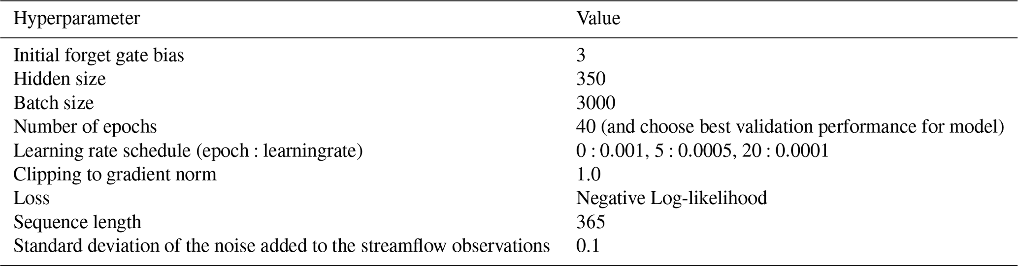
In order to find good hyperparameters for the EARLS LSTM we use a mixture of manual and grid search. The goal was to find a good trade-off between model simplicity and generalization. Table A1 shows the final parameters for the EARLS LSTM.

A2.2 Distributional predictions

In order to achieve distributional predictions we adapt the approach from Klotz et al. (2022), letting the LSTM parameterize a single asymmetric Laplacian for each time step. To get the runoff estimate within the EARLS we use the location parameter of the distribution. We do the training in normalized space (as described in Kratzert et al., 2019b). For the dataset we rescale the location and scale parameters, but leave the asymmetry parameter unchanged.

Table A1 Hyperparameter settings for the EARLS LSTM.

Appendix B: A very short introduction to mixture density networks with asymmetric Laplacian distributions

In many hydrological modeling settings, we are interested in representing predictive uncertainty in a flexible, data-driven way. One such approach are mixture density networks (MDNs), which ingest the same input as a neural network would but parametrize a distribution as output. In other words, with MDNs we can provide an distributional estimation of the runoff for each time step. Klotz et al. (2022) adopted a special form of MDN, which they coined Countable Mixture of Asymmetric Laplacians (CMAL). CMAL replaces the Gaussian components of a standard MDN with asymmetric Laplacian components. The idea here is to make the individual components of the MDN more powerful and move them closer to the conditions encountered in rainfall–runoff modeling. In CMAL, each component can express skewness and has heavier tails than a Gaussian. By mixing several such components, we can model multimodal, skewed uncertainty structures. In EARLS, however, we only use the special case CMAL, where we have a single component: An asymmetric Laplacian distribution (ALD).

An ALD is defined by the probability density function:

$$\begin{array}{}\text{(B1)}& \begin{array}{rl}\mathrm{ALD}(y\mid \mathit{\mu },b,\mathit{\tau })& ={\displaystyle \frac{\mathit{\tau }(\mathrm{1}-\mathit{\tau })}{b}}\\ & \exp \left(-{\displaystyle \frac{(y-\mathit{\mu })(\mathit{\tau }-{\mathbf{1}}_{\mathit{\{}y<\mathit{\mu }\mathit{\}}})}{b}}\right),\end{array}\end{array}$$

where μ is the location parameter (and also the mode), b>0 is the scale parameter (which controls the dispersion), and $\mathit{\tau }\in (\mathrm{0},\mathrm{1})$ is an asymmetry parameter (which defines the skewness of the distribution). For each time step t of the prediction the LSTM outputs all three parameters $\mathit{\{}\mathit{\mu },b,\mathit{\tau }\mathit{\}}$ in dependence of the received input. When τ=0.5, the ALD reduces to a symmetric Laplace distribution. For τ≠0.5, one tail becomes longer than the other, producing a skewed shape. This makes ALD components suitable for modeling asymmetric error distributions that are common in flow predictions. In the EARLS dataset we report the μ as the streamflow estimation, but also provide b and τ. Hence, the dataset provides full distributional estimations for each simulated time step.

We train our model by minimizing the negative log-likelihood of observed data:

$$\begin{array}{}\text{(B2)}& \mathcal{L}=-\sum _t\log \left(\mathrm{ALD}\left(y_t\mid \mathit{\mu }\left({\mathit{x}}_t\right),b\left({\mathit{x}}_t\right),\mathit{\tau }\left({\mathit{x}}_t\right)\right)\right).\end{array}$$

Appendix C: Further data quality checks

C1 Post hoc model examination

As a post hoc analysis of the model evaluation we investigate the relationship between model performance and (a) static inputs or (b) streamflow respectively. For this, we use the 500 basins from the test set (Appendix A1) and the basin similarity measure from Bertola et al. (2023). In their conception $\mathcal{Z}=Z_{\mathrm{1}},Z_{\mathrm{2}},\mathrm{\dots },Z_M$ is a collection of different basin attributes where each $Z_M=[z_{\mathrm{1}}^{\left(m\right)},z_{\mathrm{2}}^{\left(m\right)},\mathrm{\dots },z_N^{\left(m\right)}]$ is a vector of a given attribute m (e.g., average elevation) over the different basins M. That is, each entry in the vector is property of interest (e.g., the average elevation) for a given basin. Then, for two basins i and j the “Bertola distance” d is the Euclidean distance:

$$\begin{array}{}\text{(C1)}& d(\mathcal{Z},i,j)=\sqrt{\sum _{m=\mathrm{1}}^M\left({\displaystyle \frac{z_i^{\left(m\right)}-z_j^{\left(m\right)}}{\mathrm{sd}\left(Z_m\right)}}\right)},\end{array}$$

where sd(Z_n) denotes the standard deviation of Z_n. We make use of two different choices for 𝒵. The first set consists of the 13 static inputs of our model and the second choice depends on the streamflow only. For the latter, we choose the logarithm of the mean of the annual maximum specific streamflow following Bertola et al. (2023). That is, the annual maximum discharge normalized to a basin area of 100 km² (see Bertola et al., 2023). Formally, we can express these choices as

$$\begin{array}{}\text{(C2)}& d_a(\mathcal{Z}=S_{\mathrm{1}},S_{\mathrm{2}},\mathrm{\dots },S_{\mathrm{13}},i,j)=\sqrt{\sum _{m=\mathrm{1}}^M\left({\displaystyle \frac{s_i^{\left(m\right)}-s_j^{\left(m\right)}}{\mathrm{sd}\left(S_m\right)}}\right)},\end{array}$$

and

$$\begin{array}{}\text{(C3)}& d_b(\mathcal{Z}=\log (\stackrel{\mathrm{̃}}{Q}),i,j)=\sqrt{\sum _{m=\mathrm{1}}^M\left({\displaystyle \frac{\log \left({\stackrel{\mathrm{̃}}{q}}_i^{\left(m\right)}\right)-\log \left({\stackrel{\mathrm{̃}}{q}}_j^{\left(m\right)}\right)}{\mathrm{sd}\left(\log \right({\stackrel{\mathrm{̃}}{Q}}_m\left)\right)}}\right)},\end{array}$$

where S_i refers to the static inputs, and $\log \left(\stackrel{\mathrm{̃}}{Q}\right)$ refers to the normalized annual discharges. The distance d_a does solely depend on the static inputs and is therefore always computeable. In contrast, d_b does only depend on the runoff and can hence exclusively be used for model diagnosis in gauged basins. To understand whether particularly low or high model performance might be related to static basin attributes or runoff dynamics, we analyze two subsets of basins: basins for which NSE<0 and those for which NSE>0.8. We then compare the following sets of average distances

$$\begin{array}{}\text{(C4)}& \begin{array}{rl}{D}_{<\mathrm{0.0}}& =E_i\left(d\right(\mathcal{Z},i,j\left)\right)|i\ne j\text{and}\\ & {\text{NSE}}_i<\mathrm{0.0}\forall i,j\in \mathrm{1},\mathrm{2},\mathrm{\dots },M,\end{array}\end{array}$$

and

$$\begin{array}{}\text{(C5)}& \begin{array}{rl}{D}_{>\mathrm{0.8}}& =E_i\left(d\right(\mathcal{Z},i,j\left)\right)|i\ne j\text{and}\\ & {\text{NSE}}_i>\mathrm{0.8}\forall i,j\in \mathrm{1},\mathrm{2},\mathrm{\dots },M.\end{array}\end{array}$$

If there is a pattern between within the two subsets D_<0.0 and D_>0.8, then it could be possible to predict whether the model performs well or not – and modelers can use that information to infer whether a model performs well or not for a given basin.

C1.1 Results

We observe a shift between badly performing basins in $D_{<\mathrm{0},\mathrm{0}}$ and well performing basins in D_>0.8 (Fig. C1a). This shift is absent for the same analysis using static attributes (Fig. C1b). In fact, for the latter, the mode of the distribution is at a lower value despite comparing higher dimensional entities (i.e., the 13 static attributes). These quantitative results suggest that it is easier to discriminate the model performances with streamflow observation than with static attributes. The results also align with our hydrological justifications for model performance (Sect. 3), since anthropogenic factors are not encoded in static attributes but are reflected in the streamflow.

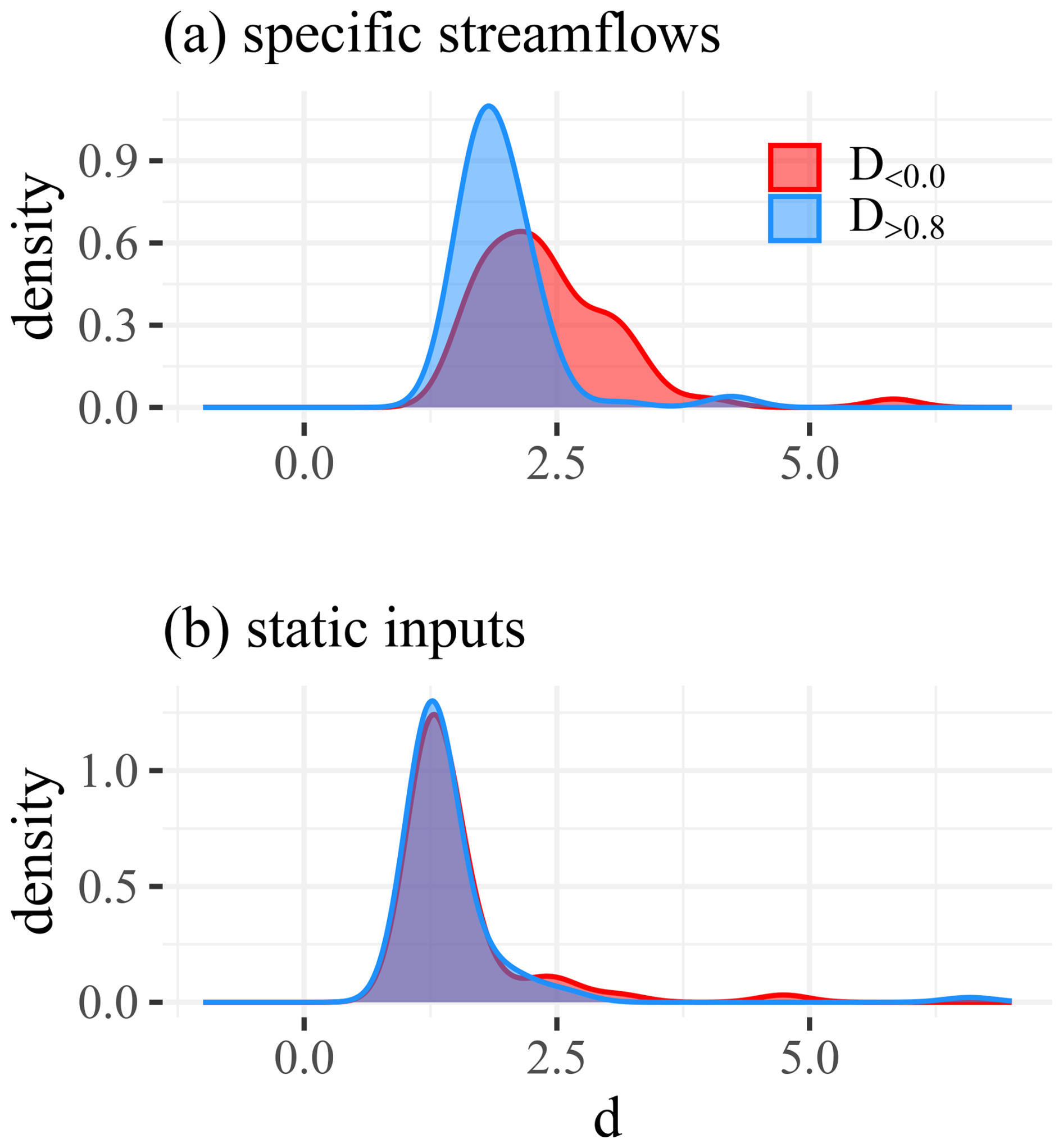
Figure C1 Comparison of the distributions of average “Bertola distances d” (Appendix C1) for the subset of basins with low NSE values (D_<0.0) and the subset of basins with high NSE values (D_>0.8). Plot (a) shows the respecitve distances for the streamflow and plot (b) fo the static inputs (Appendix C1).

C2 Model to model comparison

We use the mesoscale hydrological model (mHM; Samaniego et al., 2010; Kumar et al., 2013) as a reference model for the comparative evaluation. Specifically, we run mHM in two configurations for seperate 161 basins that are not part of EARLS. The first configuration is represented by the global parametrization from Kumar et al. (2013), hereafter referred to as “mHM default”. For the second configuration, we calibrate the parameters for each basin with 1970–1999 for training and use the years 2000–2020 for testing, hereafter referred to as “local mHM”. In both cases, we use E-OBS for the dynamical inputs (precipitation, average temperature and potential evapotranspiration estimated with the Hargreaves-Samani method (Hargreaves and Samani, 1985) and static inputs from Table C1. Since mHM is intrinsically a semi-distributed model, we set the spatial resolution of the model to 0.25°. For the local mHM, we maximize the NSE using the dynamically dimensioned search algorithm (Tolson and Shoemaker, 2007) with 1000 iterations. The comparative evaluation with the EARLS LSTM is therefore asymmetric: Firstly, the reconstructions are tested for an ungauged setting, while local mHM – as our reference model – is calibrated using a traditional time-split setting. Secondly, the mHM default is not a result of a specific calibration process for the task at hand and is hence disadvantaged.

Danielson and Gesch (2011)Hengl et al. (2017)Arino et al. (2012)Tucker et al. (2005)

Table C1 Morphological data used for the hydrological model mHM.

C2.1 Results

In terms of performance, the EARLS LSTM ranks between the mHM default and the locally calibrated mHM (Fig. C2). That is, until approximately the 15th percentile of NSE values, the EARLS LSTM performance is close to the mHM default performance, and roughly starting at the 40th percentile, it is close to the local mHM model. Else, it is somewhere in between, and for the best performing basins EARLS LSTM even outperforms the latter. All in all, we argue that these are promising results for an ungauged evaluation – especially if we keep in mind that this is an asymmetric comparison: the EARLS LSTM operates “out-of-sample” (validation in space), while mHM operates “in-sample” in space (validation in time).

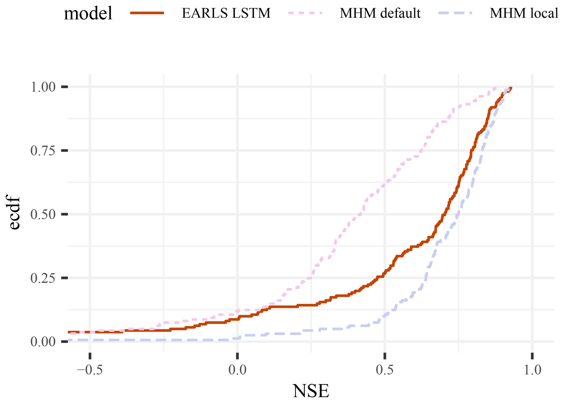
Figure C2 Empirical cumulative density functions for the comparative evaluation. The mHM default is a “best-guess” mHM calibration that summarizes many studies; the mHM local are per basin calibrated models evaluated in a traditional time-split fashion; and the EARLS LSTM represents the ungauged performance of the EARLS model.

C3 Qualitative assessment against published literature

We use EARLS to redo the core parts of the flood-timing analysis from Blöschl et al. (2017) and the flood-peak trends analysis from Blöschl et al. (2019). Both studies use observations from 1960 to 2010 (albeit the full period is not available for all gauges). We select the same timeframe and use the publicly available code from Blöschl et al. (2019) to compute the trends and spatial interpolations of the peak trends. To recreate the results of Blöschl et al. (2017) we adapt it for the flood-timing analysis according to their supplementary material (Appendix E provides details of the adoption process).

With the reproduction of the maps we want to provide a visual check for the data quality of EARLS. As far as we know, this also constitutes the first corroboration of the results from Blöschl et al. (2017, 2019) with different raw data (since the underlying raw data from the original papers are not available open access). The intrinsic limit of this assessment is that there is is no actual ground truth available. The maps from Blöschl et al. (2017, 2019) are derived by interpolating from the sparsely available gauging station data, while we get the maps from EARLS by interpolating from a denser network of gauging station (however, based on reconstructions). Hence, neither of them should be seen as absolute.

C3.1 Results

The first part of our qualitative assessment revolves around the timing of river floods in Europe. These results corresponds to Figs. 1 and 3 of Blöschl et al. (2017). We encourage readers to compare our version with these depictions since all key patterns from the original analysis are preserved in the EARLS version. Figure C3 shows the average timing of the yearly streamflow maxima from EARLS. The overall pattern of our this version closely corresponds to the original – but with a larger number of support points and a wider area of analysis. The reproduction of the corresponding analysis of flood timing trends from EARLS (Fig. C4), also mirrors the large-scale trends from Fig. 1 from the original publication. The effect of the Pyrenees, the Alps and the Carpathians are clearly visible. The 4 approximate key region with distinct drivers that Blöschl et al. (2017) highlight are also reflected in the EARLS version: (1) Northeastern Europe with earlier snowmelt; (2) the North Sea region with later winter storms; (3) Western Europe along the Atlantic coast with earlier soil moisture maxima; and (4) Parts of the Mediterranean coast (West Spain, South France, Croatia, etc.) with stronger Atlantic influence in winter.

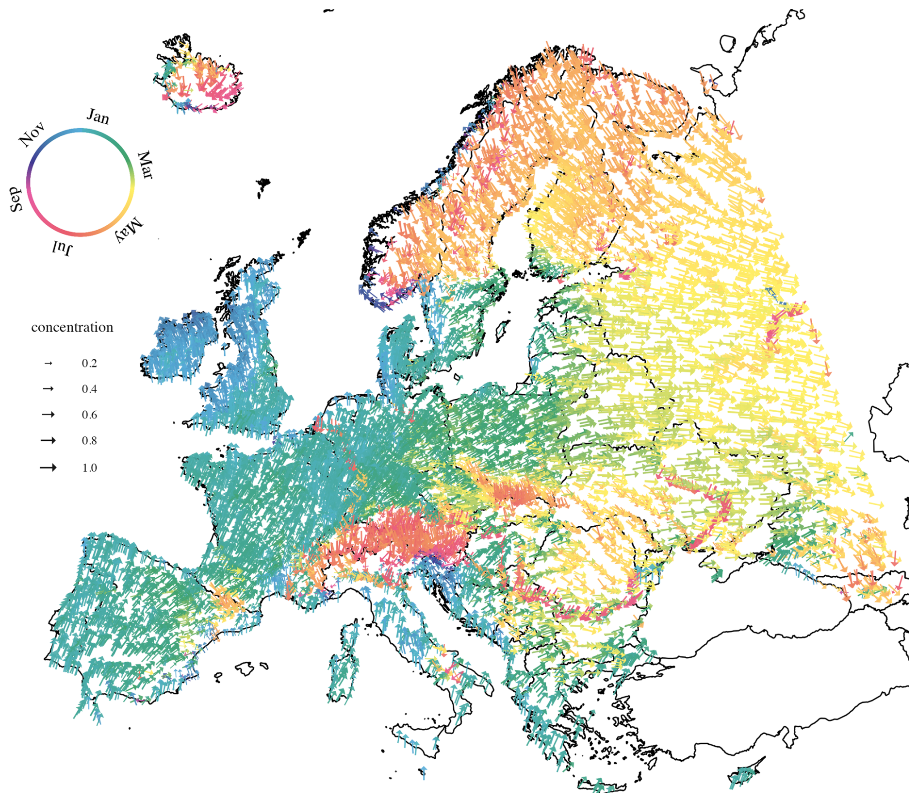
Figure C3 Reproduction of Fig. 3 from Blöschl et al. (2017) with EARLS data. Each arrow represents a basin outlet (either from a gauged or ungauged basin). Color and arrow direction indicate the average timing of floods over the period 1960–2010 (namely: light blue are winter floods; green to yellow are spring floods; orange to red are summer floods; and purple to dark blue are autumn floods). The lengths of the arrows indicate the concentration of floods (0, evenly distributed; 1, all floods occur on the same date).

The plotting data from Blöschl et al. (2019) are openly available. We can therefore directly compare them with our EARLS version. To this end, we made a reproduction of their results (Fig. C5a) and contrasted it with the corresponding EARLS version (Fig. C5b). Both show similar large-scale trends, but significant discrepancies exist for large and small-scale patterns. Scandinavia and North-East Europe have the biggest divergence in terms of large-scale patterns. There, the original version shows slightly decreasing trends in floods, while the EARLS version shows no or slightly increasing trends. In absolute terms the differences are not that large, but the extent at which the differences occur is noteworthy. The largest absolute differences, on the other hand, occur in the north of Portugal (where the EARLS version shows major negative trends) and West Russia/Ukraine (where the original analysis depicts substantially larger negative values).

Some differences can be explained by data availability (Appendix F). In general, the EARLS version appears to have more details, which, we posit, is linked to a higher number of data points used for kriging. EARLS lacks reconstructions for the Asian part of Turkey, while Blöschl et al. (2019) have observations there. Blöschl et al. (2019) have limited observations in western Russia and northern Ukraine, showing strong negative trends in flood magnitudes. EARLS has denser coverage, showing negative trends restricted to a specific eastern region. However, E-OBS is based on few observations stations in Eastern Europe (the actual number varies from variable to variable; see, e.g., Fig. 6 in do Nascimento et al., 2024). Neither of the two analyses have data in the most northern part of West Russia, resulting in flat spatial trends. Furthermore, in the data from Blöschl et al. (2019) the availability of streamflow observations varies widely from station to station, while EARLS is more homogeneous in this regard, potentially leading to different trend estimates. In summary, we argue that the results of our qualitative assessment show the merit our the EARLS data for scientific inquiry and corroborate the quality of the simulations.

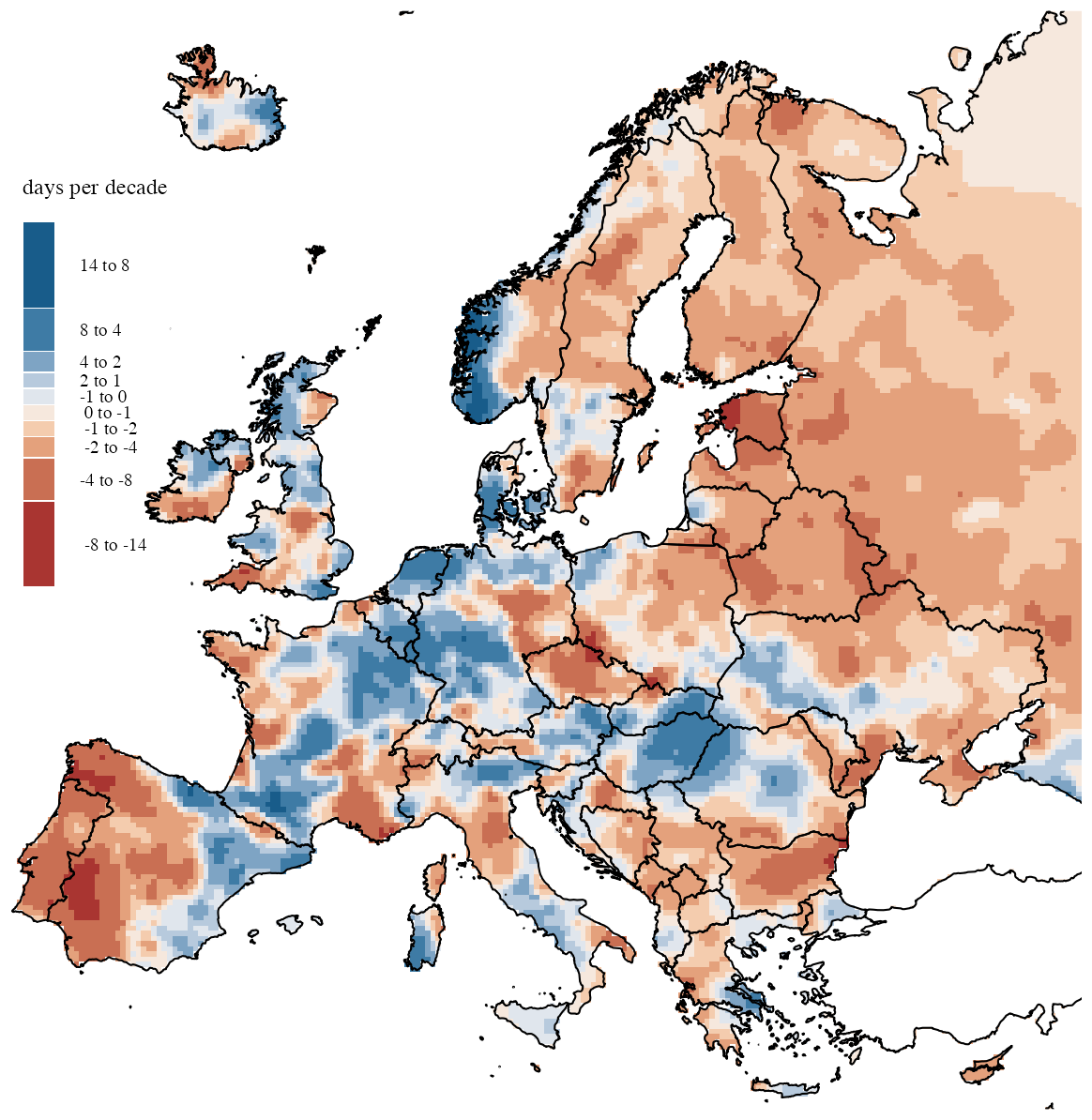
Figure C4 Our EARLS-based remake of the flood peak timing trends from Blöschl et al. (2017). Increasing trends are depicted in blue, negative trends in red. The most extreme negative trends can be spotted in Spain/Portugal and the strongest decreasing trends in the west of Norway. In general, the overall patterns match the ones from the original publication. However, they do show more detail because the interpolation is made on basis of many more supporting points than available for the original (Appendix F).

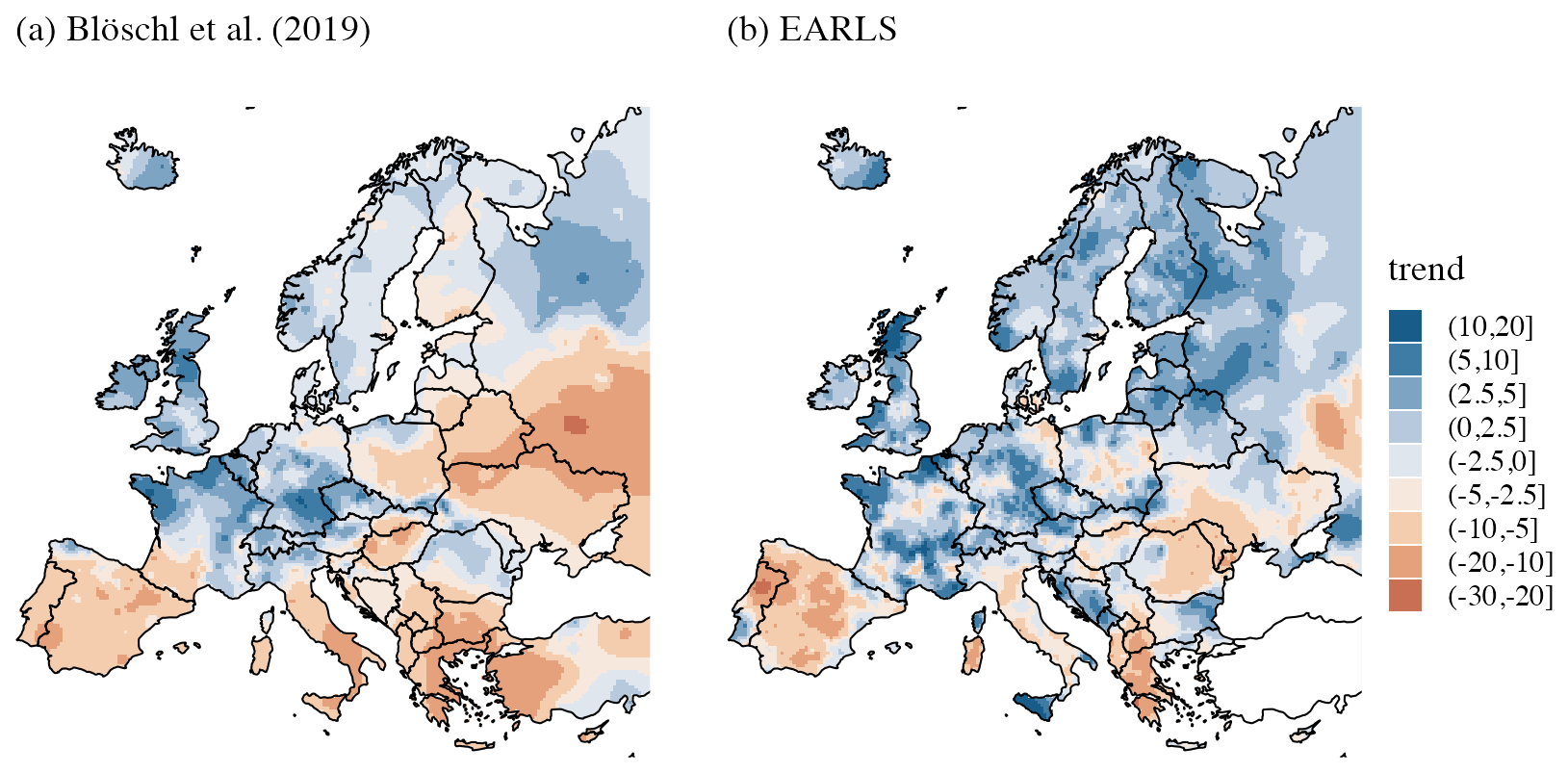
Figure C5 Comparison of the trend analysis for flood peaks from 1960 to 2010 derived from different datasets: Our reproduction with data of annual maxima from (a) Blöschl et al. (2019), and (b) EARLS. Increasing trends are in blue, decreasing ones in red. Blöschl et al. (2019) manually binned their data into specific classes. In contrast, we choose a continuous color-scale centered around zero. Blöschl et al. (2019) document the data and the original code for (a), while Klotz et al. (2026a) provides the complete plotting code and the underlying data for the figure.

Appendix D: Other metrics for evaluation

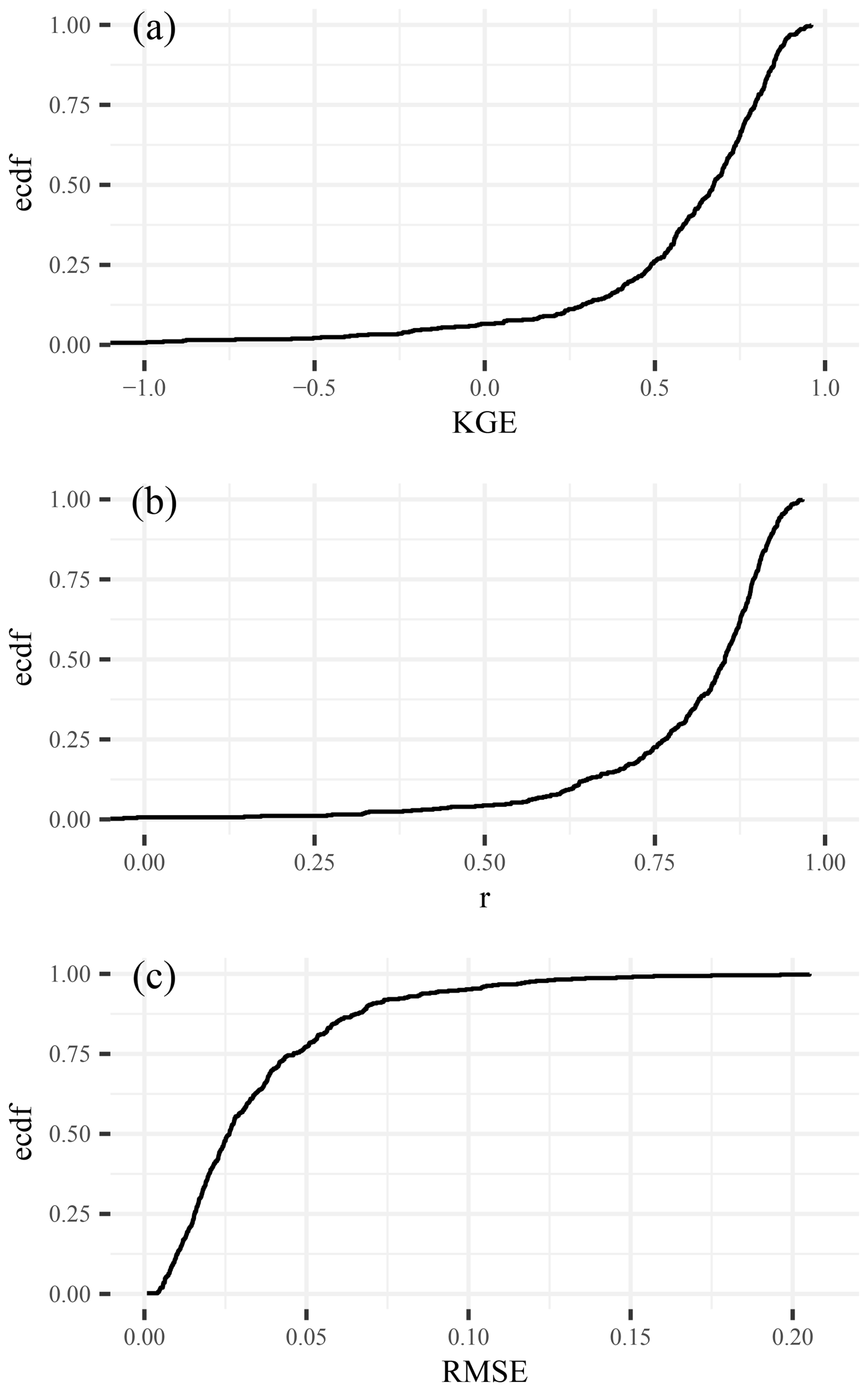
Figure D1 Empirical cumulative density function of the Kling–Gupta efficiency (KGE) for the test evaluation. Each point on the line represents the model performance for one of the 500 test basins.

This appendix shows the results for different evaluation metrics for the evaluation experiment presented in Appendix C2. Specifically, Fig. D1a shows the Kling–Gupta efficiency, (b) shows the Pearson's correlation coefficient, and (c) shows the root mean squared error.

Appendix E: Estimation of trend statistics

Our procedure for estimating the long-term trends statistics for yearly flood timing and yearly peak flow trends (Appendix C3) follows Blöschl et al. (2017) and Blöschl et al. (2019) respectively. This section partially mirrors the supplementary material Blöschl et al. (2017) and describes the technical details of our implementation.

E1 Yearly peak-flow trends

For the flood trend analysis part we follow Blöschl et al. (2017): First, we extract a series of observerations that consists of the highest peak discharge recorded in each calendar year (i.e., the annual maximum peak flow) from EARLS. Then, we estimate the trend in each series using a robust approach and interpolate the trend estimates using Kriging. Blöschl et al. (2017) only provide the data for their experiments, while Blöschl et al. (2019) provide data and R-code for their experiments. Hence, for this demonstration we modified their code to stay as close as possible to their results. The robust estimation is achieved by using the Theil–Sen slope β (Theil, 1950; Sen, 1968):

$$\begin{array}{}\text{(E1)}& \mathit{\beta }=\text{median}\left(\left\{{\displaystyle \frac{Q_i-Q_j}{i-j}}|i,j\in \mathcal{J}\text{and }i\ne j\right\}\right),\end{array}$$

where Q_z indicates the maximal streamflow of a given year z and 𝒥 contains the indices of all the years from 1960 to 2010 – which corresponds to the time span that Blöschl et al. (2019) use.

E2 Flood timing analysis and trends

The demonstration of the flood timing analysis follows Blöschl et al. (2017). Specifically, we reproduce two of their investigations: (1) an examination of long-term trend of the flood-timing and an analysis of the average flood timing over Europe (represented by Figs. 1 and 3 in Blöschl et al. (2017); and Figs. C3 and C4 in our contribution). Following their procedure, we first compute for each station the average day D within a year where peak flows have occurred during the observation period. And, to account for the cyclic nature of yearly data all calculations are performed using circular procedures/statistics. As Blöschl et al. (2017) we only take the stations for which the null hypothesis of circular uniformity (which is assessed with Kuiper's test) is rejected with a significance level of α=0.1. For this contribution no code is available. Hence, we use the description in the supplementary material to modify the code from Blöschl et al. (2019) for the trend examination. This means, that code for the average flood timing analysis is largely from ground up (according to the provided documentation from the supplementary material).

We convert date of occurrence D_i of a flood in year i into an angular value using:

$$\begin{array}{}\text{(E2)}& \mathit{\theta }={\displaystyle \frac{\mathrm{2}\mathit{\pi }}{m_i}}\text{with}\mathrm{0}\le {\mathit{\theta }}_i\le \mathrm{2}\mathit{\pi },\end{array}$$

where m_i is the number of days for year i, and D_i gives the corresponding day of the year so that D_i=1 corresponds to 1 January and D_i=m_i to 31 December.

We compute the average date of occurrence D of a flood at a station as:

$$\begin{array}{}\text{(E3)}& \overline{D}=\left\{\begin{array}{ll}{\tan }^{-\mathrm{1}}\left(\frac{\overline{y}}{\overline{x}}\right)\frac{\overline{m}}{\mathrm{365}}& \text{for}\overline{x}>\mathrm{0},\overline{y}\ge \mathrm{0},\\ \left({\tan }^{-\mathrm{1}}\left(\frac{\overline{y}}{\overline{x}}\right)+\mathit{\pi }\right)\frac{\overline{m}}{\mathrm{2}\mathit{\pi }}& \text{for}\overline{x}\le \mathrm{0},\\ \left({\tan }^{-\mathrm{1}}\left(\frac{\overline{y}}{\overline{x}}\right)+\mathrm{2}\mathit{\pi }\right)\frac{\overline{m}}{\mathrm{2}\mathit{\pi }}& \text{for}\overline{x}>\mathrm{0},\overline{y}<\mathrm{0}.\end{array}\right.\end{array}$$

Here, the arc-tangens tan ⁻¹ yields the angle in radians, x and y are the cosine and sine components of the average date, m is the average number of days per year (which we re-calculate to account the fact that some years had no data), and n is the total number of flood peaks at that station. That is:

$$\begin{array}{l}{\displaystyle }\overline{x}={\displaystyle \frac{\mathrm{1}}{n}}\sum _{i=\mathrm{1}}^n\cos \left({\mathit{\theta }}_i\right),\\ {\displaystyle }\overline{y}={\displaystyle \frac{\mathrm{1}}{n}}\sum _{i=\mathrm{1}}^n\sin \left({\mathit{\theta }}_i\right),\end{array}$$

and

$$\overline{m}={\displaystyle \frac{\mathrm{1}}{n}}\sum _{i=\mathrm{1}}^n{m}_i.$$

Lastly, Blöschl et al. (2017) define concentration R of the date of occurrence around the average date as:

$$\begin{array}{}\text{(E4)}& R=\sqrt{{\overline{x}}^{\mathrm{2}}+{\overline{y}}^{\mathrm{2}}}\text{with}\mathrm{0}\le R\le \mathrm{1}.\end{array}$$

Indeed, the mapping of $\overline{D}$ and R constitutes our reproduction of the average flood timing analysis from Blöschl et al. (2017).

E3 Trends in timing

For the timing trend estimation we use the same adjusted Theil-Sen slope estimator as reported by Blöschl et al. (2017). The computation is similar to the one given by Eq. (E1), but adds a correction factor k to account for the circularity of the task:

$$\begin{array}{}\text{(E5)}& \begin{array}{rl}{\mathit{\beta }}_{\circ }& =\text{median}\left(\left\{{\displaystyle \frac{Q_i-Q_j+k}{i-j}}|i,j\in \mathcal{J}\text{and }i\ne j\right\}\right)\\ & \text{with}k=\left\{\begin{array}{ll}-\overline{m}& \text{if}{D}_j-D_i>\overline{m}/\mathrm{2},\\ \overline{m}& \text{if}{D}_j-D_i<-\overline{m}/\mathrm{2},\\ & \mathrm{0}\text{ otherwise}.\end{array}\right.\end{array}\end{array}$$

Here, the Theil-Sen slope β_∘ has units of days per year. Thus to get an estimate for the 10 year period reported in Blöschl et al. (2017) it has to be scaled accordingly. Lastly, we used the same Kriging approach as we do for the yearly peak-flow trends to get a map of the large-scale spatial patterns within Europe.

Appendix F: Locations

If we compare the “location”/support points for kriging between Blöschl et al. (2017, 2019) and EARLS we can see that the latter uses many more location points to supported the interpolation (Fig. F1). To provide a rough estimate about the difference in density we count the number of basins within a box around Scandinavia (colored dots in Fig. F1). In that case we get approximately 300 for the location points from Blöschl et al. (2017, 2019), and around 2500 simulated stations locations in the same box for EARLS (note: for the former count we rounded up in the decimal, while for the latter we rounded down in the hundreds). However, an analyst might still feel uncomfortable to use reconstructions that are not at gauging station that was used for model training or too far away from such a station station. The “coordinates.csv” file of EARLS (Sect. 4) contains two columns to provide assistance for such circumstances: The “basintype” provides a flag for gauged and ungauged basins (the former were used for training, the latter not) and the “nearest_gauged_distance” column provides the Euclidean distance to the nearest gauged station computed from the latitude and longitude. As shown in Fig. F2 this allows analysts to demarcate region where the reconstructions are supported on solid ground truth data – i.e., Western and Northern Europe – from reconstructions that are not – i.e., Eastern and Southeastern Europe.

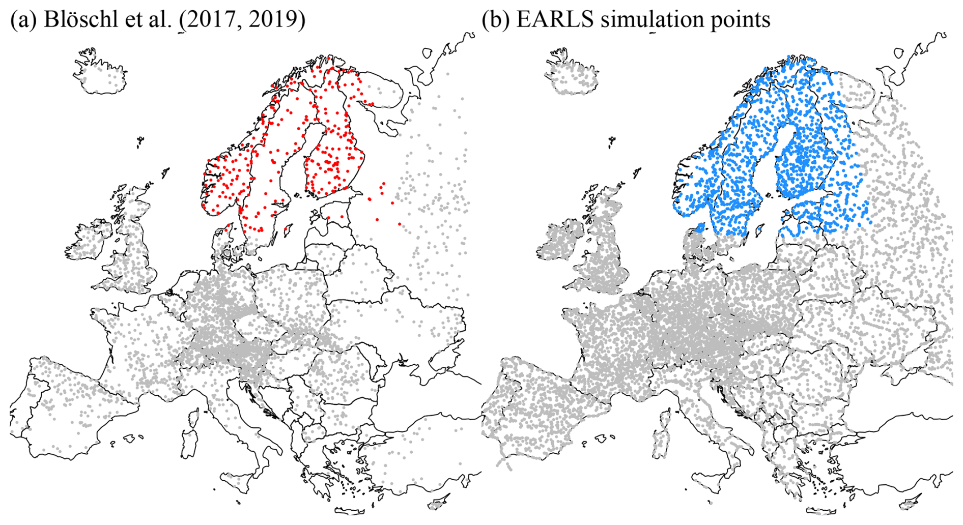
Figure F1 Comparison of the available of location/support points for the kriging-based interpolation. Plot (a) shows the reference points from Blöschl et al. (2017, 2019) and plot (b) the simulated station from EARLS. The colored areas in both (a) and (b) refer to the same area of the data based on a box a given latitude and longitude. For the former it contains approximately 300 points, for the latter around 2500.

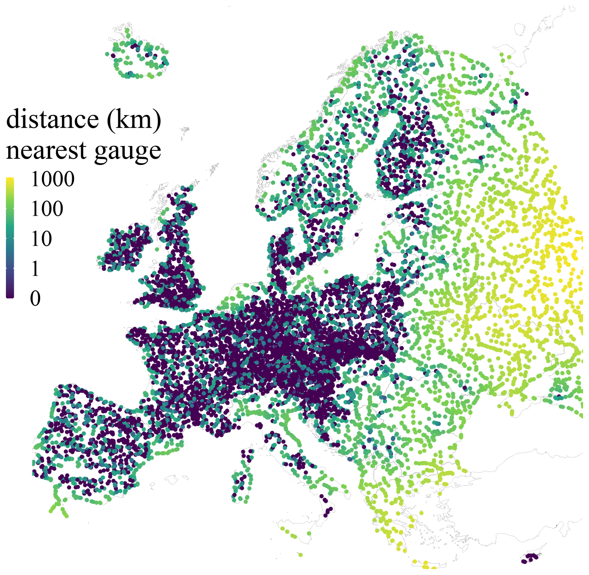
Figure F2 Distance to nearest gauged station. Points represent simulation sites, with the color indicating the Euclidean distance to the nearest gauged station. In the plot, gauged sites (that we used for training) and those near them appear near the lower end of the color scale, while points that are far away from stations that have been used during the training on the higher.