Mapping three decades of urban growth in China: a 30 m annual building height dataset (1990–2019)

Long-term building height data are critical for analyzing urban morphological evolution and renewal processes, yet such datasets at fine spatial resolutions remain scarce for large geographical regions. This study proposes a framework to generate continuous annual building height maps for China at 30 m spatial resolution from 1990 to 2019, integrating multi-source remote sensing data (Landsat, Sentinel-1/2, etc.) through the eXtreme Gradient Boosting (XGBoost) model. The framework reconstructs Vertical-Vertical (VV) band, incorporates reference data derived from the Continuous Change Detection and Classification (CCDC) algorithm, and utilizes Total Variation (TV) denoising to achieve temporal consistency, while retaining inter-annual building height variations. Validation results demonstrate the stable performance of the building height maps over the past three decades, with nationwide RMSE values ranging between 3.20 and 4.27 m. Comparisons confirm that our results are consistent with reference height datasets and capture the temporal evolution of building heights driven by urban development and renewal. Furthermore, our dataset shows pronounced horizontal and vertical expansion of Chinese cities between 1990 and 2019, as the total impervious surface area increases from 54 407.03 to 170 595.06 km² and overall building volume rises from 365.98 to 882.43 km³. Provincial contributions to national building volume change substantially over time, with Hebei (11.3 %), Shandong (10.6 %), and Heilongjiang (10.2 %) leading in 1990, while Shandong (9.8 %), Hebei (9.5 %) and Guangdong (9.4 %) are in the leading positions in 2019. The resulting annual 30 m resolution building height datasets, made openly accessible, provide a valuable foundation for cross-city comparisons, long-term three-dimensional (3D) urban morphology studies, and policy-relevant planning in fast-growing Chinese cities. The dataset is available at https://doi.org/10.6084/m9.figshare.29918978 (Zhang et al., 2025b).

1 Introduction

Building height, a fundamental metric of buildings, captures the vertical dimension of urban form as shaped by both human activity and the natural environment. Accurate mapping of building height enhances human settlement analyses and applications, such as 3D population distribution modeling (Alahmadi et al., 2013), material stock quantification (Frantz et al., 2023), and well-being assessments (Schug et al., 2021). It also facilitates quantitative evaluation of interactions between buildings and natural environment, including urban heat island effects (Huang and Wang, 2019; Yang et al., 2021; Yu et al., 2025), pollution dispersion dynamics (Lyu et al., 2024), and energy consumption patterns (Resch et al., 2016). Moreover, temporal variations in building height reflect both construction and demolition activities, indicating vertical morphological transformations during urbanization (Cohen, 2015). Monitoring these changes is essential for understanding urban expansion and renewal, characterizing urban growth patterns, and guiding sustainable urban planning (Peters et al., 2022; Yu et al., 2026).

Optical and Synthetic Aperture Radar (SAR) satellite data have become indispensable for large-scale building height mapping due to their seamless spatiotemporal coverage with multi-dimensional land-surface information. Optical remote sensing data generally exploit shadows and morphological profiles to extract heights of various buildings (Qi et al., 2016). For instance, Geiß et al. (2020) applied ensemble regression to map building heights across four German cities using Sentinel-2 high-resolution optical imagery. Similarly, Sun et al. (2024) established a footprint-level Chinese building height dataset using Beijing-3 Very High Resolution (VHR) optical imagery combined with deep learning methods. SAR data serve as another important source for building height mapping, as microwave backscatters closely relate to building heights (Koppel et al., 2017). Li et al. (2020b) utilized Sentinel-1 Vertical-Vertical (VV) and Vertical-Horizontal (VH) band data to produce an urban height dataset covering 96 U.S. cities. However, a single remote sensing data type often provides insufficient spectral or structural information, limiting the extraction accuracy of building heights. For example, optical data become unreliable in cloud-covered regions (Koppel et al., 2017), while SAR data tend to be noisy in areas with tall buildings (Yadav et al., 2025).

Recent research increasingly integrates optical and SAR remote sensing data to generate building height products, harnessing their complementary strengths. For instance, Frantz et al. (2021) combined Sentinel-1 SAR with Sentinel-2 optical imagery to map building heights nationwide in Germany, while Yadav et al. (2025) generated a 10 m resolution map for four European countries using a deep learning model on Sentinel-1/2 time series data. Ancillary datasets, such as nighttime lights and population data, are also incorporated as covariates, improving building height estimation by capturing building characteristics and surrounding environmental contexts from multiple perspectives. Wu et al. (2023) produced China's first 10 m resolution national building height dataset by fusing Sentinel-1/2 imagery, nighttime light observations, and Digital Surface Model (DSM) data. Che et al. (2024) further advanced the field by integrating multi-source remote sensing data with architectural geometric features to produce the first global footprint-level building height dataset with an XGBoost model. Despite these advances, most existing datasets remain static, mapping building heights for only a single year due to limited reliable reference data. In addition, the restricted temporal span of high-resolution satellite systems such as Sentinel-1/2 hampers detailed historical mapping, particularly before 2010.

Constructing long-term building height datasets requires multi-temporal remote sensing observations. Frolking et al. (2022) developed a global microwave backscatter coefficient dataset from multiple scatterometers spanning 1993–2020, yet its 0.05° spatial resolution (roughly equivalent to 5 km at the equator) limits its applicability for microscale urban analysis. Higher-resolution, long-term building height mapping has been pursued through machine and deep learning methods that integrate multi-source, multi-decadal datasets. Using a morphology-based method, He et al. (2023) produced a global 30 m resolution building height dataset from 1990 to 2010 by fusing Advanced Land Observing Satellite (ALOS) DSM with the Landsat-derived Global Artificial Impervious Area (GAIA) data. Yan et al. (2024) trained a random forest model on 2019 building height reference data, Landsat optical imagery, and socioeconomic variables, directly applying it to other years and thereby generating 1 km resolution height estimates for 2001–2019 across China. Nevertheless, these datasets largely neglect not only urban renewal but also complicated urban building and demolition processes. They are unreliable for regions undergoing frequent demolition–reconstruction cycles, where historical height records often deviate substantially from present conditions.

To account for urban renewal processes, Wang et al. (2023) proposed a temporal segmentation algorithm applied to Landsat time series, identifying urban renewal zones in Beijing and interpolating heights from 1990 to 2020 using logistic reasoning. However, this approach relied on manually selected thresholds, limiting its extrapolation to other regions. Chen et al. (2025) addressed these limitations by generating reliable height reference data across multiple years and fully exploiting long-term Landsat observations. They integrated spaceborne LiDAR data from the Global Ecosystem Dynamics Investigation (GEDI) as height benchmarks. Reference height data were then extracted for specified years using the Continuous Change Detection and Classification (CCDC) algorithm to detect land use change, and a deep learning method was applied to Landsat archives to map building heights. This framework produced 30 m resolution building height datasets for China in 2005, 2010, 2015, and 2020. Nevertheless, it depends on Phased Array L-band Synthetic Aperture Radar (PALSAR) data, which cover only limited years (2007, 2009–2010, 2015, 2019–2020), making height mapping for the intervening years a challenging task.

Continuous annual building height datasets are crucial for detecting building demolition and reconstruction at fine spatio-temporal scales during urban growth and renewal. However, existing long-term building height datasets either lack scalability to broader spatial extents or fail to capture year-to-year changes. To address this gap, this study aims to generate annual building height maps for China from 1990 to 2019 at 30 m resolution. First, we establish a framework based on the eXtreme Gradient Boosting (XGBoost) model that integrates multi-source, multi-temporal, and multi-decadal remote sensing data (including optical, SAR, and terrain information) for long-term building height estimation. The VV band is reconstructed from 1990 to 2014 to enhance estimation accuracy, providing continuous signals that reflect latent building-height features. Second, to account for urban renewal, the CCDC algorithm is applied to generate annual reference height data through land-use transition detection, and the Total Variation (TV) denoising is utilized to improve the stability and reliability of building height time series. Finally, the accuracy of long-term building height mapping is evaluated through comparisons with existing datasets and historical satellite imagery, while the mapped spatio-temporal dynamics of building height and volume provide additional evidence of the dataset's ability to accurately represent urban growth and renewal.

2 Datasets

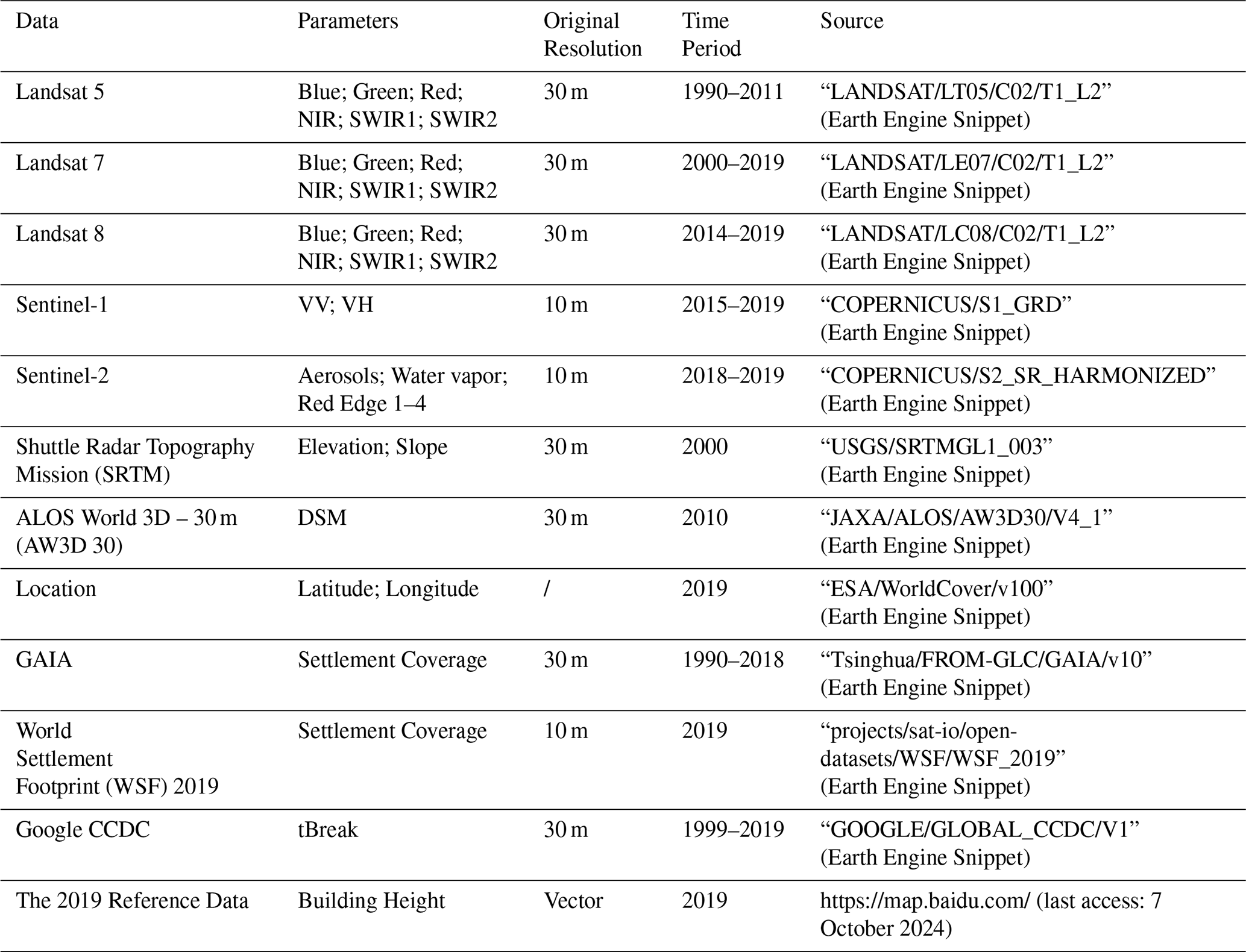
Remote sensing data we used is from multiple public access Earth observation sources, including optical data, radar data, terrain data and products derived from satellite imagery. All data preprocessing procedures are conducted on the Google Earth Engine (GEE) platform (Gorelick et al., 2017). GEE is a cloud platform hosting public satellite imagery and derived products (e.g. Landsat, Sentinel, SRTM) with scalable server-side processing. Details of the datasets acquired and preprocessed on GEE are provided in Table 1.

Table 1 Data utilized to map long-term building heights.

2.1 Landsat images

Landsat surface reflectance time series data from 1990 to 2019 is utilized. It has been atmospherically corrected through the Landsat Ecosystem Disturbance Adaptive Processing System (LEDAPS) (Masek et al., 2006) and Land Surface Reflectance Code (LaSRC) (Vermote et al., 2016). The spectral bands include Blue, Green, Red, Near Infrared (NIR), Shortwave Infrared 1 (SWIR1), and Shortwave Infrared 2 (SWIR2). Five more indices are further derived: the Normalized Difference Vegetation Index (NDVI), as defined in Eq. (1); the Enhanced Vegetation Index (EVI), given by Eq. (2); the Land Surface Water Index (LSWI) from Eq. (3); the Modified Normalized Difference Water Index (MNDWI) according to Eq. (4), and Normalized Difference Built-up Index (NDBI) in Eq. (5). These indices' predictive validity has been demonstrated in previous researches (Wu et al., 2023; Li et al., 2020a):

$$\begin{array}{}\text{(1)}& {\displaystyle }\mathrm{NDVI}={\displaystyle \frac{{\mathit{\rho }}_{\mathrm{NIR}}-{\mathit{\rho }}_{\mathrm{red}}}{{\mathit{\rho }}_{\mathrm{NIR}}+{\mathit{\rho }}_{\mathrm{red}}}},\text{(2)}& {\displaystyle }\mathrm{EVI}={\displaystyle \frac{\mathrm{2.5}\left({\mathit{\rho }}_{\mathrm{NIR}}-{\mathit{\rho }}_{\mathrm{red}}\right)}{({\mathit{\rho }}_{\mathrm{NIR}}+\mathrm{6}{\mathit{\rho }}_{\mathrm{red}}-\mathrm{7.5}{\mathit{\rho }}_{\mathrm{blue}}+\mathrm{1})}},\text{(3)}& {\displaystyle }\mathrm{LSWI}={\displaystyle \frac{{\mathit{\rho }}_{\mathrm{NIR}}-{\mathit{\rho }}_{\mathrm{SWIR}\mathrm{1}}}{{\mathit{\rho }}_{\mathrm{NIR}}+{\mathit{\rho }}_{\mathrm{SWIR}\mathrm{1}}}},\text{(4)}& {\displaystyle }\mathrm{MNDWI}={\displaystyle \frac{{\mathit{\rho }}_{\mathrm{green}}-{\mathit{\rho }}_{\mathrm{SWIR}\mathrm{1}}}{{\mathit{\rho }}_{\mathrm{green}}+{\mathit{\rho }}_{\mathrm{SWIR}\mathrm{1}}}},\text{(5)}& {\displaystyle }\mathrm{NDBI}={\displaystyle \frac{{\mathit{\rho }}_{\mathrm{SWIR}\mathrm{1}}-{\mathit{\rho }}_{\mathrm{NIR}}}{{\mathit{\rho }}_{\mathrm{SWIR}\mathrm{1}}+{\mathit{\rho }}_{\mathrm{NIR}}}},\end{array}$$

where ρ_NIR, ρ_red, ρ_blue, ρ_SWIR 1 and ρ_green each equals the pixel value of the corresponding band in Landsat. Images from Landsat 5 Thematic Mapper (TM), Landsat 7 Enhanced Thematic Mapper Plus (ETM+), and Landsat 8 Operational Land Imager/Thermal Infrared Sensor (OLI/TIRS) are concatenated to form a long-term dataset. Cloud-covered pixels are masked using the QA_PIXEL band. For each year's available imagery, three statistical composites are computed per pixel: median reflectance values representing central tendency, maximum values capturing spectral extremes, and standard deviation quantifying temporal variability (Wu et al., 2023).

2.2 Sentinel-1 and Sentinel-2 data

VV and VH backscatters in Sentinel-1 SAR data are selected for building height mapping during 2015–2019, with the VV backscatter subsequently serving as reference data later for 1 km VV backscatter reconstruction. For Sentinel-2 multispectral imagery, six distinctive bands absent in Landsat sensors are utilized to enhance height estimation accuracy for the 2018–2019 period: Red Edge 1–4, Aerosol and Water Vapor. Cloud masking is implemented using the QA60 quality assessment band, followed by median value compositing to generate annual cloud-free Sentinel-2 reflectance products.

2.3 Terrain data

The ALOS World 3D-30 m (AW3D30) DSM and the Shuttle Radar Topography Mission Digital Elevation Model (SRTM DEM) are integrated. While the SRTM DEM serves as the primary topographic predictor for building height mapping, the AW3D30 DSM contributes to 1 km VV backscatter reconstruction. Although DSMs like AW3D30 are widely adopted in single-year height estimations (Huang et al., 2022), their constrained temporal coverage (2006–2011) introduces chronological inconsistencies in long-term estimations. DEM data is deliberately selected since it predominantly captures terrain geometry rather than structures above surface. Furthermore, longitude and latitude are incorporated as additional predictors to account for spatial heterogeneity effects across China's vast territory (Yan et al., 2024).

2.4 Human settlement footprint

Two global human settlement footprint products are used: GAIA (Gong et al., 2020) and WSF (Marconcini et al., 2021). World Settlement Footprint (WSF) dataset, initially at 10 m spatial resolution, is resampled to 30 m to match our analytical grid. These datasets are applied to keep our research area within human settlement, with GAIA used for 1990–2018 and WSF 2019 for 2019.

2.5 Google global Landsat-based CCDC segments

The CCDC algorithm has been widely adopted for identifying temporal patterns of land-use transitions (Hu et al., 2024; Stanimirova et al., 2023). The Google CCDC dataset is generated by applying the algorithm proposed by Zhu and Woodcock (2014) to the complete Landsat image archive from 1999 to 2019, generating multi-layered outputs that include temporal breakpoint detection, observation counts, and breakpoint confidence levels. The original algorithm achieves a producer's accuracy of 97.72 %, user's accuracy of 85.60 %, and overall accuracy of 91.80 %, demonstrating its reliability. The CCDC change detection results are employed as a temporal filter to exclude recently renewed urban areas from reference data.

2.6 The 2019 reference data

The 2019 reference data for building heights are derived from building footprint records of that year from Baidu Maps, covering 59 Chinese cities. As the original data provide only building floor counts, they are converted into height estimates by multiplying by 3 m per floor. The 3 m-per-floor conversion is a statistically robust approximation for grid- level aggregation supported by different researches, although being unable to fully capture localized floor-height variations in specialized structures (Zhang et al., 2025a; Wu et al., 2023). This dataset has been validated by Liu et al. (2021), reporting 86.8 % vertical accuracy with a mean height deviation of approximately 1 m.

To generate rasterized reference data for 2019, vector footprints are converted to 1 m resolution height raster to preserve height details. Then, these raster datasets are resampled to 30 m, averaging the value of every 1 m × 1 m pixel within the 30 m × 30 m pixel (Zhou et al., 2022).

$$\begin{array}{}\text{(6)}& H^{\mathrm{30}\mathrm{m}}={\displaystyle \frac{{\sum }_i^{\mathrm{900}}{H}_i^{\mathrm{1}\mathrm{m}}}{\mathrm{900}}}={\displaystyle \frac{{\sum }_j^{\mathrm{nbc}}{H}_j^{\mathrm{1}\mathrm{m}}}{\mathrm{900}}},\end{array}$$

where $H_i^{\mathrm{1}\mathrm{m}}$ denotes the height value of each 1 m sub-pixel. Non-building sub-pixels are assigned a value of 0, so the numerator is equivalent to the sum of height values over building-covered sub-pixels only, denoted as $H_j^{\mathrm{1}\mathrm{m}}$ . Here, nbc represents the number of building-covered 1 m sub-pixels among the 900 sub-pixels within the grid. The denominator is kept as 900 rather than nbc, because using nbc would produce a building-footprint-only mean height and could assign comparable values to grids with similar building heights but different building coverage fractions, thereby failing to capture variations in built-up intensity.

Although non-building 1 m sub-pixels are included in this calculation, the 30 m grids are constrained using the GAIA impervious surface mask and building information, excluding grids without any building information during reference sample preparation. After these procedures, the 2019 reference height dataset contains 9 780 241 sample pixels across China, with the largest city contributing 1 165 620 pixels (Fig. 1). Zero-height samples are omitted during model training so that the training data represent building-related areas. These 30 m grids are used as the basic units for subsequent processing, model training, validation, and dataset generation, corresponding to the 30 m pixels in the final building height dataset.

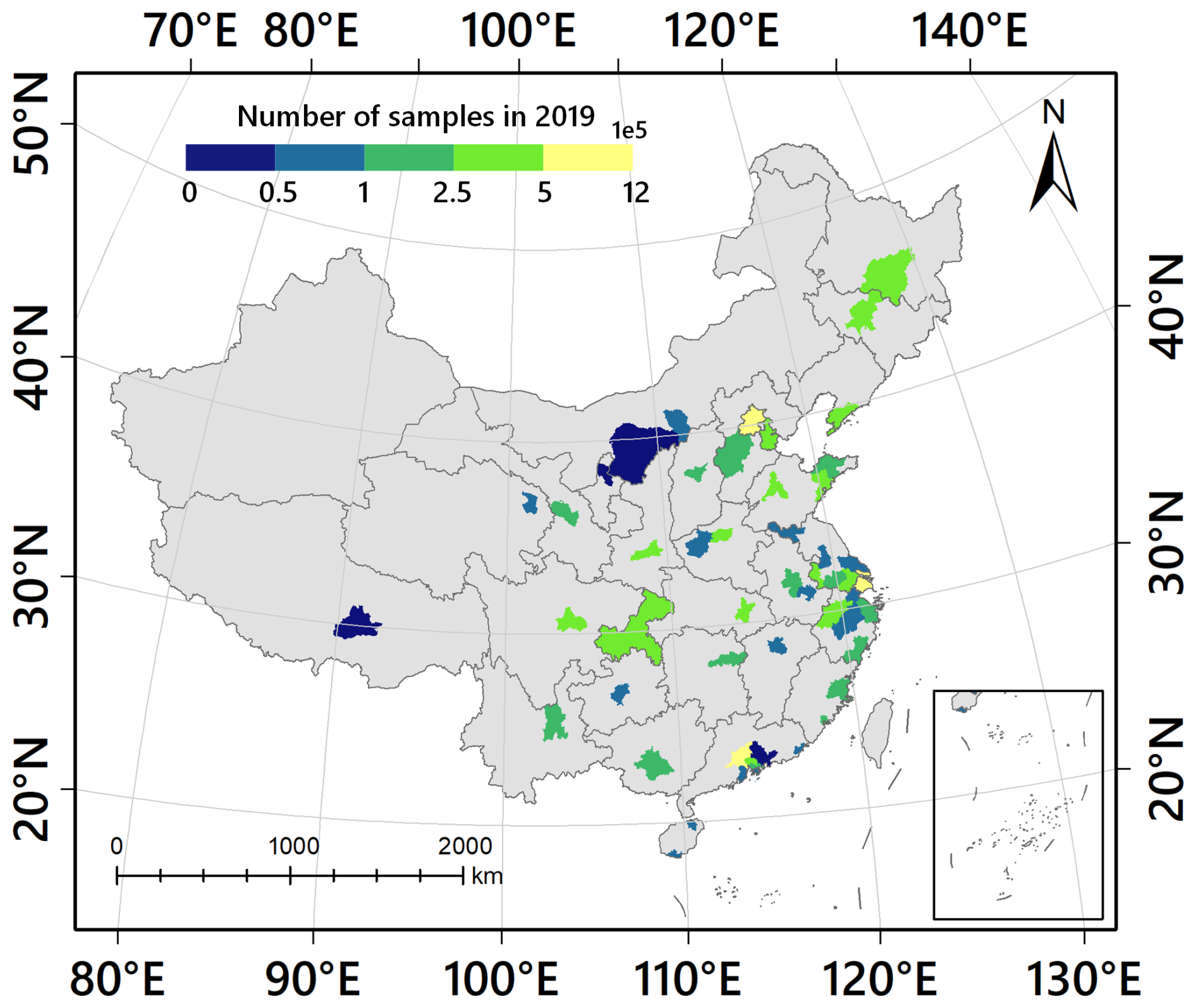
Figure 1 Number of sample pixels in 2019 in every sampled city.

With these constraints, the derived height better captures the combined effects of building height and building coverage. This grid-level calculation is consistent with established practices in large-scale urban morphology studies (Chen et al., 2025; Li et al., 2020a; Zhou et al., 2022) and aligns with the Gross Building Height concept in the GHSL framework (Pesaresi et al., 2024).

3 Method and validation

The proposed method consists of four main steps (Fig. 2). First, to obtain reference building heights for years prior to 2019, the study area is delineated using GAIA and WSF 2019 settlement datasets, and reference samples for each year are extracted by Google CCDC Segments. To address the limited temporal coverage of SAR data, long-term VV backscatter at 1 km spatial resolution for 1990–2014 is constructed by Random Forest model based on Landsat spectral indices and SRTM DEM (Fig. 2a). Data is then augmented to compensate for the lack of high-rise building in reference data. Second, XGBoost-based height regression models are trained for each year from 1990 to 2019 according to the annual reference data, and TV denoising is applied to post-process (Fig. 2b). Third, the accuracy of the models is evaluated and compared (Fig. 2c), and the patterns of urban building growth and renewal are analyzed (Fig. 2d).

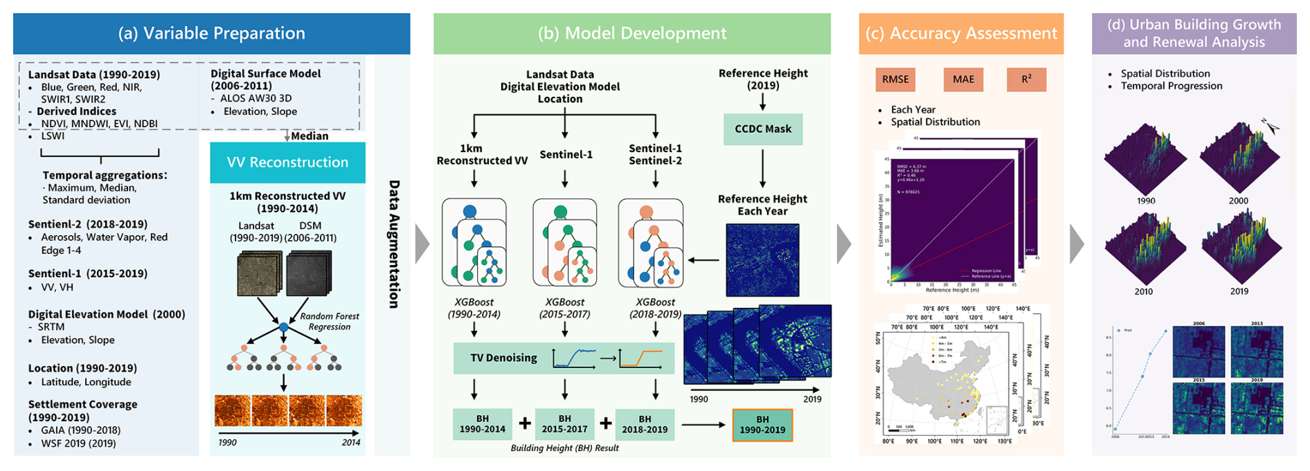
Figure 2 The framework for annual building height mapping. (a) Variable preparation; (b) Model development; (c) Accuracy assessment; (d) Urban building growth and renewal analysis.

3.1 Variable preparation

3.1.1 Annual reference building heights from 1999 to 2019

This study employs three basic types of land-use conversion scenarios established in previous literature (Huang et al., 2020b; Stilla and Xu, 2023; Zhao et al., 2023), to generate annual reference building heights that account for urban renewal. The scenarios are defined as follows:

1. New construction: areas transition from non-building land cover (e.g., water, grassland, barren land) to built-up/impervious land, characterized by the emergence of new buildings and an increase in height from zero.

2. Complete demolition: areas transition from building to non-building, defined by the removal of structures, resulting in a decrease in height to zero.

3. Persistent built-up: areas with no land-use conversion, where building heights generally remain stable. Minor variations may occur due to the reconstruction of existing structures.

Urban renewal is represented by the combined effect of these conversion types, capturing distinct trajectories of building height change.

New construction areas are identified using the GAIA and WSF 2019 settlement datasets. Complete demolition areas are inherently absent from the 2019 reference data. However, GAIA and WSF 2019 cannot capture demolition process, as they only identify new impervious surfaces and neglect conversions from building to non-building. To address this limitation, the CCDC is applied to identify persistent built-up areas based on the 2019 reference data. These areas are then used to derive annual reference building heights (Huang et al., 2020a).

The CCDC mask records time of the last detected breakpoint. For a given year, only pixels with no breakpoint within the time period between this year and 2019 are kept as the reference data for this year. The absence of a breakpoint implies a high probability that these pixels experience no land-use transitions, therefore buildings within are neither newly constructed nor demolished, and thus retain the building height from the 2019 reference data. Given a target historical year t ($\mathrm{1990}\le t\le \mathrm{2018}$) and pixel (x, y), the annual reference height H_t(x, y) is determined by:

$$\begin{array}{}\text{(7)}& H_t\left(x,y\right)=\left\{\begin{array}{ll}{H}_{\mathrm{2019}}\left(x,y\right)& \text{if}{T}_{\mathrm{break}}\left(x,y\right)=\mathrm{0}\text{or}\\ & T_{\mathrm{break}}\left(x,y\right)<t\\ \text{Excluded}& \text{otherwise}\end{array}\right.\end{array}$$

where T_break(x, y) is the latest breakpoint year detected by the CCDC algorithm for that pixel, with 0 meaning no breakpoint detected. This method guarantees that the 2019 reference height is only projected backward to year t if the land surface has remained spectrally stable and undisturbed since year t. If any spectral breakpoint is detected within the window [t, 2019], the pixel is completely excluded from the training-validation pool for year t.

Although CCDC data cover the period from 1999 to 2019, China's urbanization before 1999 was predominantly new district development rather than systematic urban renewal (Wu, 2016). Consequently, the 1999 CCDC masks are uniformly applied to 1990–1999, which may introduce minor yet non-negligible uncertainty to the pre-2000 period, keeping the overall accuracy around 65 %. Chen et al. (2025) adapted a similar approach of extracting long-term building height labels using CCDC dataset, with labels derived from 2020 to 2005, 2010 and 2015 achieving accuracy of over 85 %, granting the reliability of applying CCDC to obtain annual reference data.

3.1.2 Reconstruction of VV band

Radar backscatters are widely utilized to develop building height datasets since they often bear valuable height information (Li et al., 2020a; Yadav et al., 2025; Wu et al., 2023; Frantz et al., 2021). However, the access of long-term high-resolution open-source radar data is of great limitation due to security reasons. Sentinel-1, as the main source of radar at present, only covers the time period since 3 October 2014.

To acquire long-term radar data, the Random Forest regression framework is adapted to fit 1 km-resolution Sentinel-1 VV backscatter with Landsat spectral bands and terrain information (Yuan et al., 2024). It achieved satisfactory performance (RMSE = 1.5 dB) in the Beijing-Tianjin-Hebei region.

The regression framework is further extended nationwide in this study, and the regressed VV backscatter is utilized as an independent variable in subsequent XGBoost-based models for building height mapping. The nationwide robustness of the 1 km reconstructed VV backscatter is confirmed through validation across diverse geographic regions characterized by different urban forms, local climates, and topographic conditions. Detailed accuracy metrics are provided in Table S6 in the Supplement. The predictor matrix includes six primary spectral bands (Blue, Green, Red, NIR, SWIR1, SWIR2), four indices (NDVI, EVI, MNDWI, NDBI), DEM, and DEM-derived slope. The reconstruction process is illustrated in Fig. S4 in the Supplement.

3.2 Data Augmentation

The original height distribution of reference samples is highly imbalanced, with low-rise buildings accounting for the majority. This imbalance may limit the model's ability to accurately estimate relatively high buildings. Although equal-proportion resampling can balance different height intervals, it reduces the representation of the original majority class and leads to a decline in prediction accuracy for the most prevalent building types (Moraes et al., 2024). To improve the model's performance for high-rise buildings while preserving its accuracy for dominant low-rise structures, a ratio-controlled resampling strategy is adopted.

Specifically, building heights are divided into four intervals based on reference samples: (0 m, 10 m], (10 m, 30 m], (30 m, 60 m], and (60 m, 140 m]. The sample size of each height interval above 10 m is adjusted through down-sampling or oversampling and capped at one-tenth of that of the (0 m, 10 m] category (Chawla et al., 2002; Naboureh et al., 2020). As the number of newly added pixels through oversampling exceeds the number of pixels removed through down-sampling, the total sample size increases. Although the proportion of the (10 m, 30 m] interval decreases, the experiment shows no negative effect on model accuracy. This strategy maintains the prediction accuracy for predominant low-rise buildings and simultaneously enhances the representation of high-rise samples, thereby improving the model's ability to estimate taller buildings.

3.3 Model training

XGBoost models are adopted due to their demonstrated computational efficiency and predictive accuracy in prior building height mapping studies (Che et al., 2024; Stipek et al., 2024). For each year, an independent XGBoost model is trained with year-specific variables extracted from remote sensing data, paired with corresponding reference building heights derived from CCDC masks. This approach maximizes the utility of annual data characteristics in the mapping process.

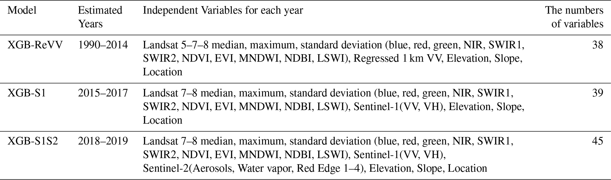
Given the limited temporal coverage of observation data, the set of predictor variables varies across years. Accordingly, three model configurations are constructed (Table 2). XGB-ReVV is applied from 1990 to 2014, using 15 predictors including Landsat spectral bands, reconstructed VV, elevation, slope, and location. XGB-S1 is employed for 2015–2017, replacing reconstructed VV with Sentinel-1 VV and VH backscatter. XGB-S1S2 is used for 2018–2019, further incorporating Sentinel-2 spectral bands in addition to the variables used in XGB-S1.

Hyperparameter optimization is conducted using Ray Tune exclusively on the 2019 dataset, and the optimized parameters are subsequently fixed to all earlier years.

Table 2 Independent variables used for different time periods.

3.4 Model evaluation

Model performance is quantified by three metrics: Root Mean Square Error (RMSE, Eq. 8), Mean Absolute Error (MAE, Eq. 9), coefficient of determination (R², Eq. 10), and relative Root Mean Square Error (rRMSE, Eq. 11). Ordinary Least Squares (OLS) regression is performed to calculate the correlation between estimated and reference height values. The annual reference building height data are split into training and testing sets, utilizing 90 % and 10 % of the samples, respectively:

$$\begin{array}{}\text{(8)}& {\displaystyle }\mathrm{RMSE}=\sqrt{{\displaystyle \frac{{\sum }_{i=\mathrm{1}}^n{\left(H_{i,\mathrm{est}}-H_{i,\mathrm{ref}}\right)}^{\mathrm{2}}}{n}}},\text{(9)}& {\displaystyle }\mathrm{MAE}={\displaystyle \frac{{\sum }_{i=\mathrm{1}}^n\left|H_{i,\mathrm{est}}-H_{i,\mathrm{ref}}\right|}{n}},\text{(10)}& {\displaystyle }{R}^{\mathrm{2}}=\mathrm{1}-{\displaystyle \frac{\left(n-\mathrm{1}\right){\sum }_{i=\mathrm{1}}^n{\left(H_{i,\mathrm{est}}-H_{i,\mathrm{ref}}\right)}^{\mathrm{2}}}{\left(n-\mathrm{2}\right){\sum }_{i=\mathrm{1}}^n{\left(H_{i,\mathrm{est}}-H_{i,\mathrm{ref}}\right)}^{\mathrm{2}}}},\text{(11)}& {\displaystyle }\mathrm{rRMSE}={\displaystyle \frac{\mathrm{RMSE}}{\frac{{\sum }_{i=\mathrm{1}}^n{H}_{i,\mathrm{ref}}}{n}}}\end{array}$$

where n equals the number of testing samples, H_i,ref equals the reference height value of the ith sample point, and H_i,est equals the estimated value.

3.5 Post process

The temporal evolution of building height at individual pixels theoretically follows a stepwise pattern: prolonged stability separated by vertical changes (construction/demolition) within a few years. However, independent annual predictions introduce arbitrary year-to-year errors unrelated to actual structural changes, causing inaccurate fluctuations within really short time periods.

To mitigate year-to-year errors, we adapt TV denoising, an approach from signal processing. Given annual sampling from 1990–2019, the height trajectory for each pixel can be interpreted as a 30-point discrete signal. TV denoising smooths these signals to preserve temporal continuity while retaining legitimate changes.

As an example of post-process, the original result before denoising in Fig. 3 shows visible fluctuation between 2007 and 2008, despite minimal differences between the Landsat images from those years in Zhongguancun, Beijing. After TV denoising, the result becomes stable, aligning with the visual observation. The TV regularization parameter (λ=5) is empirically calibrated to balance noise suppression and edge preservation.

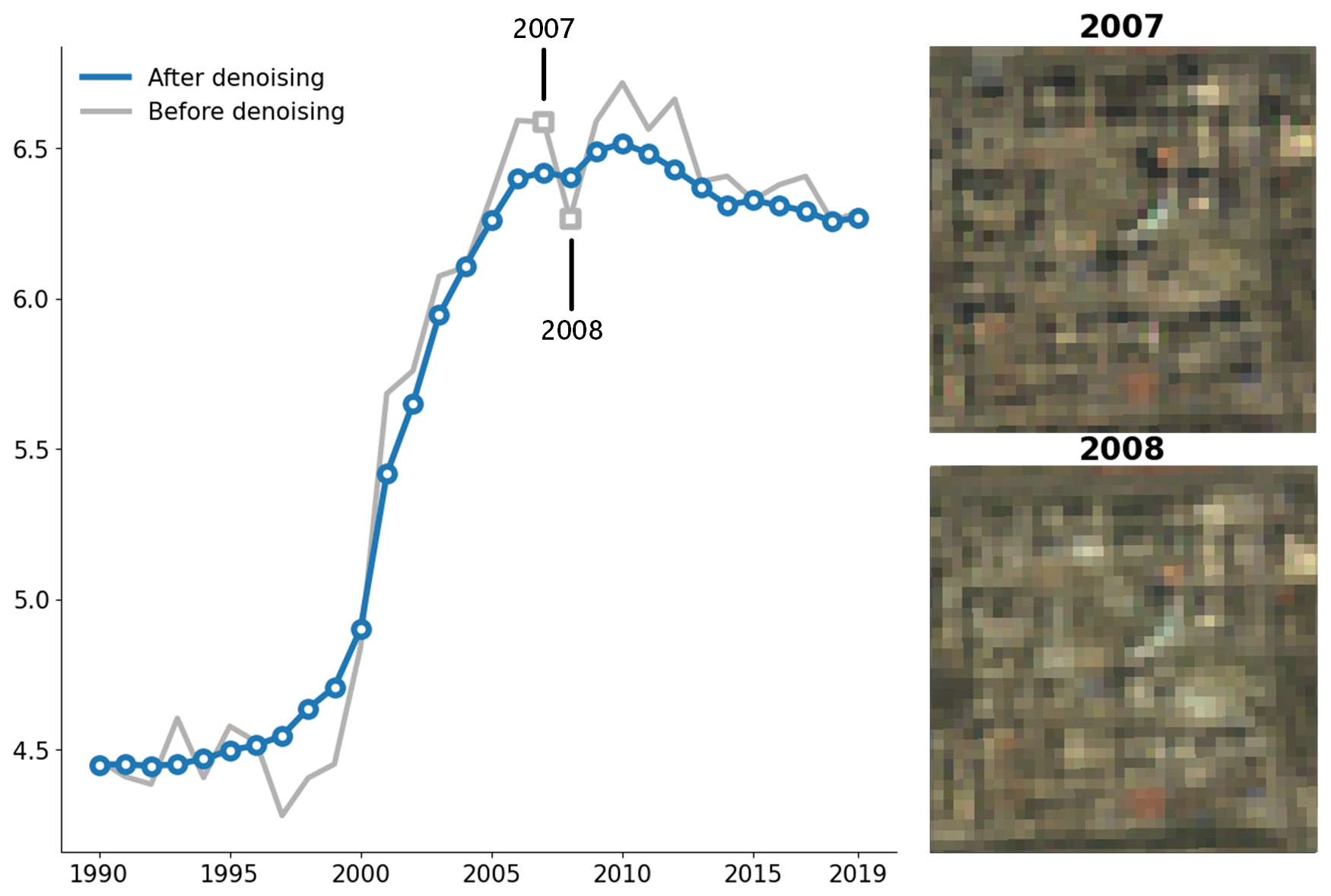
Figure 3 Effect of denoising in the sample region of Zhongguancun, Beijing. Credit: NASA/USGS Landsat.

4 Results and discussion

4.1 Accuracy of reference samples for annual building heights

The original reference height in 2019 has a total of 9 780 241 sample pixels. After extracted by CCDC and built-up area footprints, the number of sample pixels gradually decreases each year, reaching 2 293 565 sample points by 1990 (Fig. 4a). The proportion of buildings of different heights also changes each year. From 2019 back to 1990, the proportion of low-rise buildings below 10 m gradually increases, from 73.3 % to 75.1 %, while the proportion of mid- to high-rise buildings above 10 m continuously decreases. The proportion of high-rise buildings between 30–60 m and above 60 m remains relatively small throughout. The highest sample is at 139 m from 2003 to 2019, and 118 m from 1990 to 2002, demonstrating the existence of high-rise buildings in the samples. After data augmentation, reference pixels in 2019 rise to 12 401 142, decreasing to 2 925 078 by 1990 (Fig. 4b). The proportion of buildings of different height is constrained to 76.9 %, 7.7 %, 7.7 % and 7.7 %. The detailed sample counts for each year are recorded in Table S1.

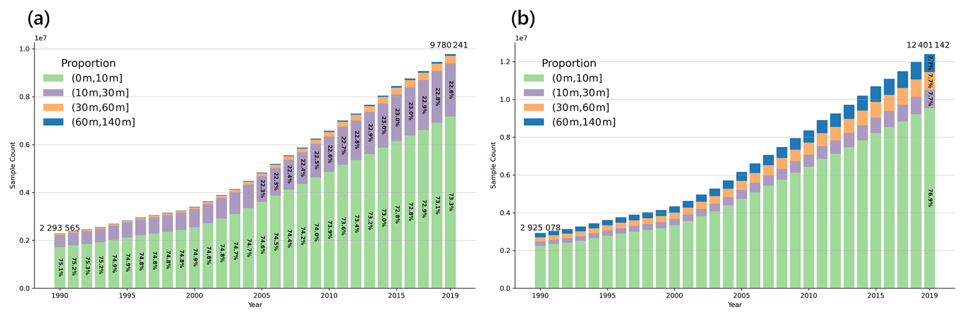
Figure 4 Number of reference samples and height proportion each year. (a) Number and proportion before augmentation; (b) Number and proportion after augmentation.

Housing transaction data obtained from house agent website Lianjia (https://lianjia.com, last access: 1 February 2026) is utilized to validate the accuracy of annual samples (Wang et al., 2023). This data provides the coordinates of each transaction's community point and the community's construction year, covering 25 out of the 59 sample cities (Fig. 5c). Since a single coordinate generally corresponds to non-building areas such as roads, water bodies, or vegetation within a community, the CCDC breakpoint year and the settlement footprint year are set over the 3×3 pixels neighborhood around each coordinate point, and the larger value between the two is selected as the marked-up year. Only starting from the marked-up year is a sample point incorporated into the annual reference height data, therefore sample points with their marked-up years larger than their construction years are regarded as true samples. Figure 5 demonstrates the result of validation. Most of the reference samples are extracted after the construction time, while samples around 2005 to 2015 are slightly more being incorrectly identified within a 5-year period (Fig. 5a). The accuracy gradually decreases from 2019 to 2002, eventually reaching a low point of 65.28 % in 1993 after a slight increase. From 1990 to 2002, the accuracy remained around 65 % (Fig. 5b). Overall, the reference samples are relatively reliable, supporting the regression process later. The exact number of validated samples and accuracy can be acquired in Table S2.

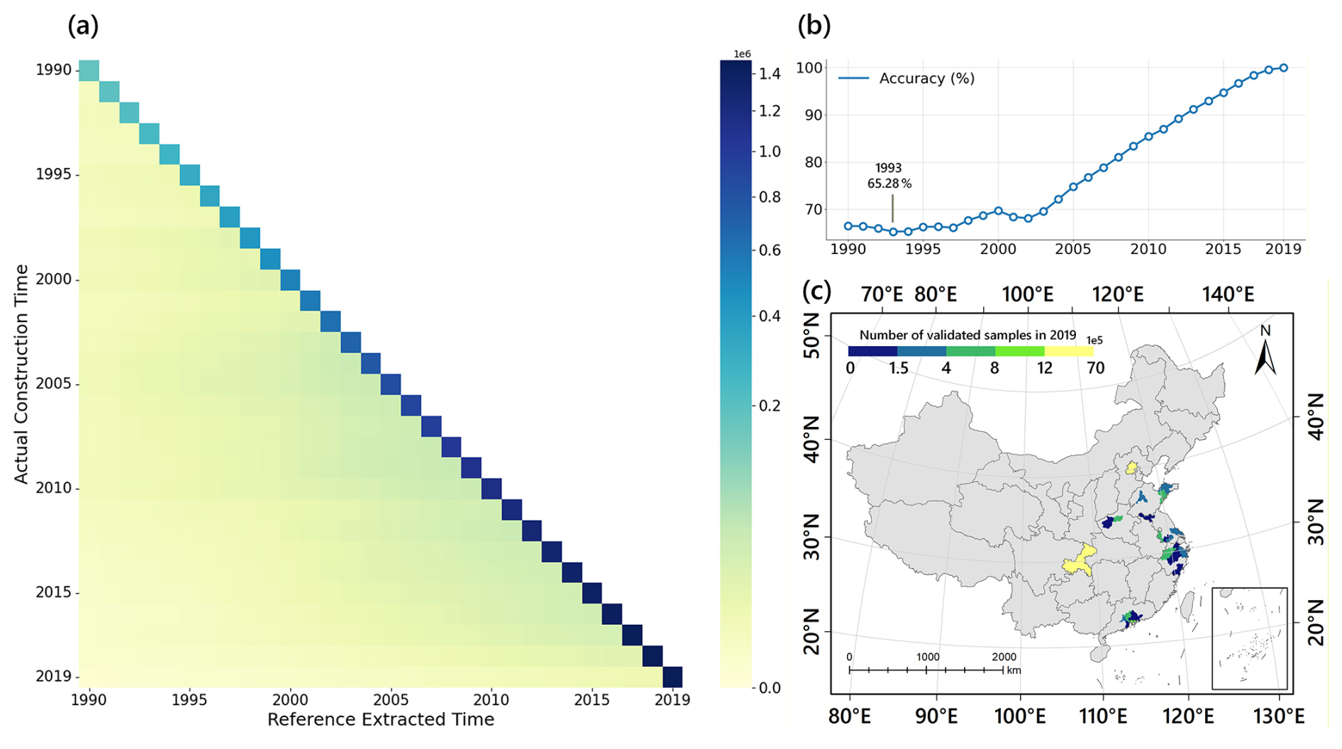
Figure 5 Results of sample validation. (a) Confusion matrix for reference time and actual construction time; (b) Accuracy of reference samples each year; (c) Number of validated samples in sampled cities.

4.2 Accuracy assessment of models

4.2.1 Performance of annual building height mapping models

Annual building height mapping results show consistency with reference building heights across the research time period. From 1990 to 2019, the RMSE of XGBoost-based models (XGB-ReVV, XGB-S1 and XGB-S1S2) ranges from 3.20 to 4.27 m, while the MAE varies between 2.27 and 2.95 m (Fig. 6a). Accuracy indices exist a temporal progression: moving backward from 2019, both RMSE and MAE first increase with fluctuations, peak in 2011, then decrease until 2000, and finally relatively stabilize between 1990–2000. The error increase likely comes from limited availability of high-resolution remote sensing data sources in earlier years. The subsequent decrease and stabilization may reflect the diminishing annual reference data quantities due to CCDC masking, and decreasing proportions of high-rise buildings that cause higher estimating variations (Chen et al., 2025). The R² fluctuates around 0.80 from 1990 to 2019 with a maximum amplitude of 0.04 (Fig. 6b), implying stable capacity of the models to explain height variance using remote sensing predictors as temporal distance increases. Overall speaking, aside from the temporal tendency, the observed temporal variability in model accuracy remains constrained within modest thresholds. The peak-to-trough ratios measure 89.5 % for RMSE, 91.3 % for MAE and 84.7 % for R². All metrics demonstrate sustained relative stability across the three-decade. The detailed RMSE, MAE, and R² values for each year are listed in Table S3.

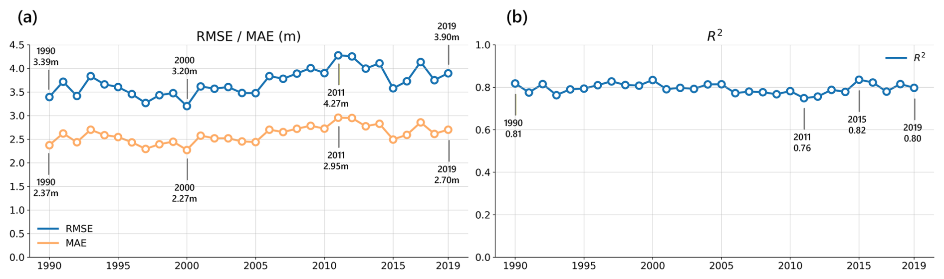
Figure 6 Model accuracy for each year. (a) the RMSE and MAE of XGBoost-based models from 1990 to 2019; (b) the R² of XGBoost-based models from 1990 to 2019.

The accuracy of the three XGBoost-based models is further evaluated for three representative years: XGB-ReVV in 2014, XGB-S1 in 2017, and XGB-S1S2 in 2019 (Fig. 7). These years correspond to the initial years of XGB-ReVV, XGB-S1, and XGB-S1S2, with each model employing a distinct set of predictor variables. Since each 30 m grid represents the area-weighted height of buildings and surrounding built-up surfaces, height values greater than 0 m but lower than 3 m may occur when buildings occupy only a limited proportion of the grid area, rather than indicating the absence of buildings. Accordingly, for visualization purposes only, the starting points of both the x- and y-axes are set to 0 m in Fig. 7.

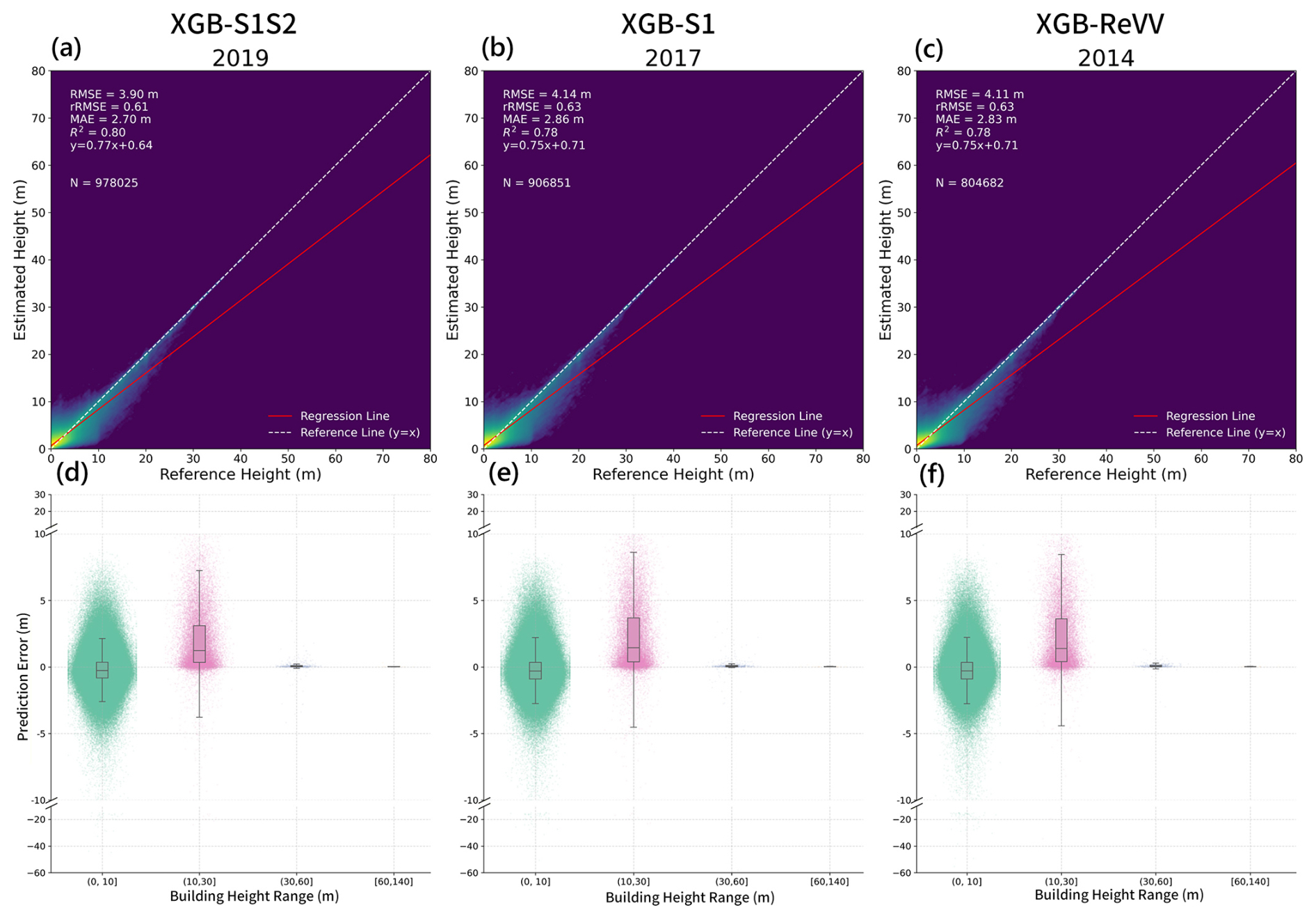
Figure 7 Accuracy of XGBoost-based models in their initial years. (a, d) XGB-S1S2 (2019); (b, e) XGB-S1 (2017); (c, f) XGB-ReVV (2014).

The prediction accuracy remains relatively consistent across these years, with RMSE values of 3.90, 4.14, and 4.11 m; MAE values of 2.70, 2.86, and 2.83 m; R² values of 0.80, 0.78, and 0.78; and rRMSE values of 0.61, 0.63 and 0.63, respectively (Fig. 7a–c). Linear regression slopes between reference and estimated heights are 0.77, 0.75, and 0.75 with intercepts of 0.64, 0.71, and 0.71 m. The minimal intercepts indicate negligible baseline offsets for low-rise structures. The slopes indicate a systematic underestimation of high-rise buildings, with predicted heights reaching only approximately half of the actual values. This limitation has been highlighted in several previous studies (Frantz et al., 2021; Che et al., 2024; Cao and Weng, 2024). Notably, the higher sample density in the low-height range of the density plot is expected, mainly due to the area-weighted definition of grid-level height, the dominance of low-rise buildings and sparsely built-up areas in the reference samples, and the visualization mechanism of the density scatter plot. This pattern does not indicate that the model is limited to predicting low-height buildings, nor does it imply that mid- or high-rise building samples are excluded from the validation. The height-stratified analysis of prediction errors shows that the models with ratio-controlled resampling achieve high accuracy for buildings exceeding 30 m, whereas structures below 30 m exhibit relatively lower accuracy (Fig. 7d–f). The results from linear regression and height-stratified analysis for each year from 1990 to 2019 are presented in Figs. S1 and S2.

4.2.2 Spatial distribution of accuracy indices

Significant regional discrepancies in prediction accuracy are observed across the 59 training cities using the 2019 model. A distinct north-south performance difference emerges (Fig. 8). Northern cities such as Beijing (RMSE = 3.82 m, MAE = 2.71 m, R² = 0.75) and Lanzhou (RMSE = 3.48 m, MAE = 2.50 m, R² = 0.66) show better performances than average metrics, while southern counterparts have both out-performing cities like Yangzhou (RMSE = 2.93 m, MAE = 2.15 m, R² = 0.33), and significantly underperforming cities like Xiamen (RMSE = 5.24 m, MAE = 2.98 m, R² = 0.38). Cities in the Pearl River Delta exhibit particularly low accuracy, like Guangzhou (RMSE = 12.51 m, MAE = 7.67 m, R² = −1.68), and Foshan (RMSE = 12.31 m, MAE = 7.73 m, R² = −1.96). These regional disparities may be attributed to meteorological factors – frequent cloud cover and precipitation in southern China likely degraded optical remote sensing data quality, thereby introducing noise into the prediction models (Zhang and Weng, 2016). Accuracy assessments for each training-sample city for every year from 1990 to 2019 are recorded in Table S4.

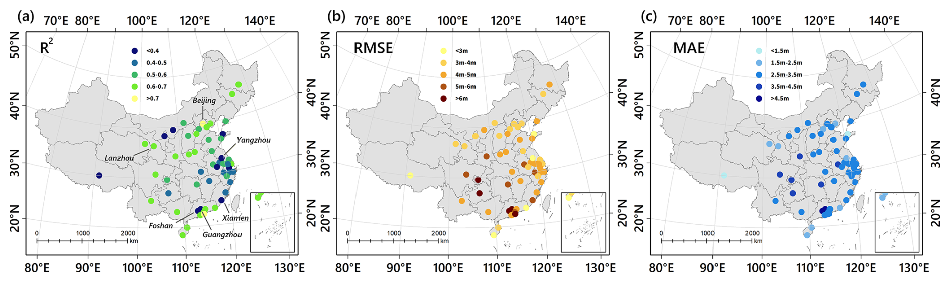
Figure 8 Distribution of accuracy indices across cities in 2019. (a) R²; (b) RMSE; (c) MAE.

4.2.3 Cross-city transferability assessment

To further evaluate the spatial transferability and cross-city robustness of the models, an independent validation is conducted using sparse building height information collected from the Lianjia real-estate platform (Fig. 9). After being matched and processed with CMAB building footprints (Zhang et al., 2025a), the Lianjia data provide community-level building heights. Since these data are neither pixel-level nor footprint-level ground truth, they are not used for model training. Instead, they provide an independent benchmark for evaluating model performance in extrapolated cities that are excluded from the reference samples.

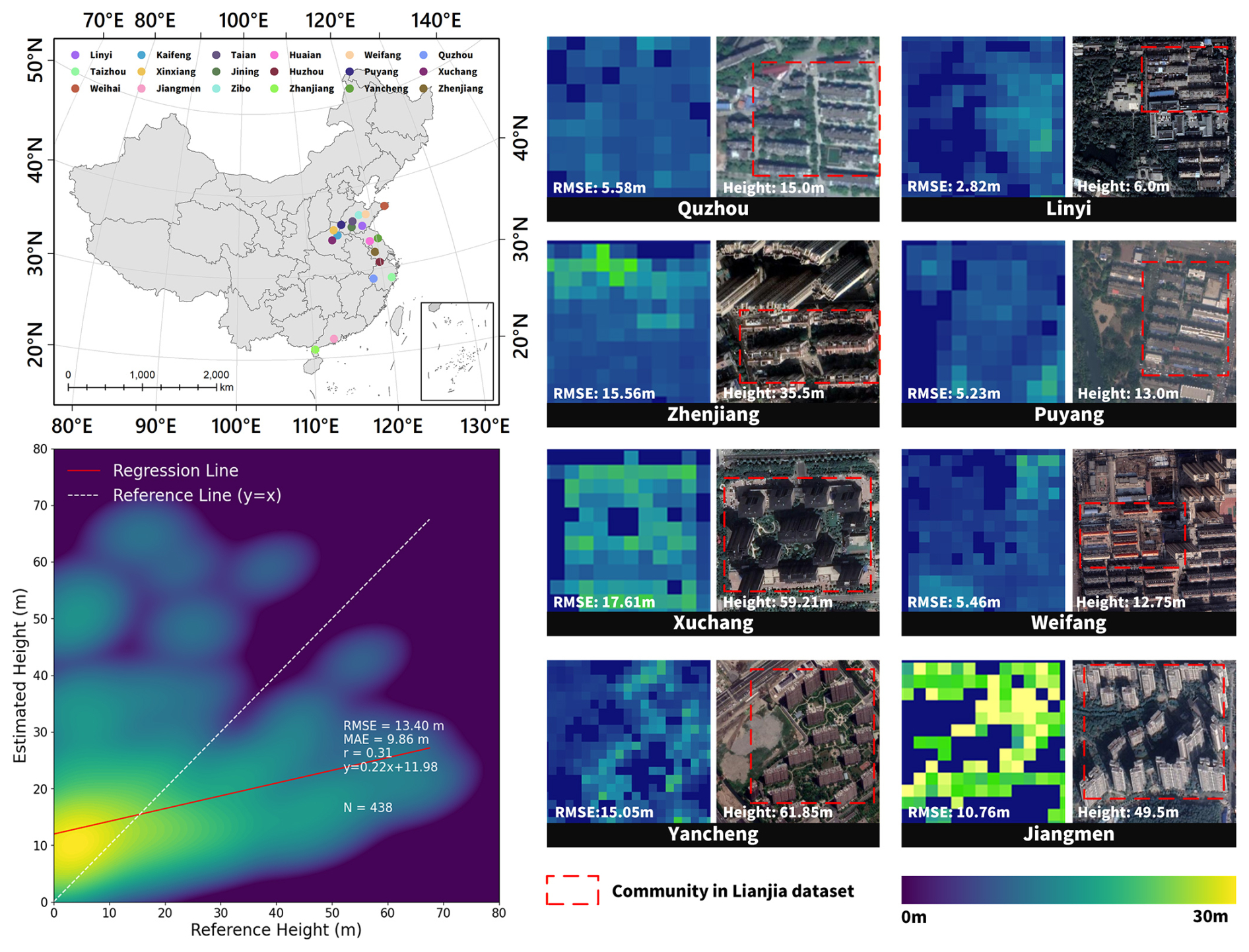
Figure 9 Accuracy assessment of model performance in cities excluded from the reference samples using Lianjia real-estate data. Satellite imagery is from © 2019 CNES/Airbus, Maxar Technologies, Google.

The extrapolation validation is conducted using the XGB-S1S2 model trained with the 2019 reference samples, because this validation only requires a single-year cross-sectional assessment. The results show that this model maintains reasonable estimation performance in cities excluded from the reference samples, with an overall RMSE of 13.40 m. For representative cities, the RMSE values are mostly within 3–6 m in low-rise built-up areas, including Linyi, Puyang, Weifang, and Quzhou. For mid- and high-rise areas, the RMSE values range from 10 to 17 m in Jiangmen, Zhenjiang, Yancheng, and Xuchang.

The relatively larger errors for taller buildings are consistent with patterns reported in existing large-scale building height studies. Che et al. (2024) show that high-rise buildings tend to contribute more strongly to regional errors; for example, in Africa, the RMSE for buildings above 50 m reaches 25.52 m, which is much higher than that for buildings below 20 m. Therefore, although underestimation still occurs in some high-rise areas, the extrapolation results remain comparable to existing findings and demonstrate this model's cross-city applicability and generalization capability.

4.3 The importance of variables

To evaluate the contributions of different variables derived from multi-source satellite imagery, predictor importance is quantified for three representative years: 2014, 2017, 2019. Correspondingly, XGB-ReVV, XGB-S1, and XGB-S1S2 are trained for these years (Fig. 10a). For Landsat bands and derived indices represented by three temporal composites (maximum, median, standard deviation), the mean importance of these composites is calculated per spectral feature. Geographic coordinates demonstrate the highest predictive importance, with latitude achieving values of 0.291, 0.320, and 0.231 across the three years, and longitude reaching 0.043, 0.075, and 0.130. Sentinel-2 spectral bands exhibit visible contributions: Red Edge 4 (0.029), Aerosol (0.018), Red Edge 1 (0.011), and Water Vapor (0.011). In radar data, Sentinel-1's VV polarization shows higher importance (0.174 in 2019, 0.160 in 2017) compared to VH (0.016 and 0.026). After replacing with reconstructed 1 km VV backscatter, its importance is 0.070. DEM elevation (0.026, 0.029, 0.013) maintains consistent relevance before introducing reconstructed 1 km VV. In conclusion, location variables (latitude/longitude) dominate predictive capacity, followed by Sentinel-1 VV backscatter, DEM elevation, and selected optical bands including Sentinel-2 Red Edge 1/Aerosols alongside Landsat NIR. Despite optical sensors providing numerous spectral variables, most exhibit limited individual importance.

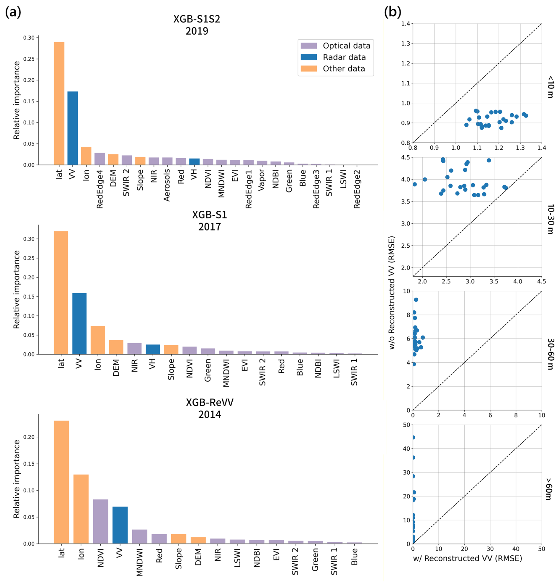
Figure 10 Importance evaluation of variables. (a) Relative importance of different variables; (b) RMSE differences between models with and without reconstructed VV.

Geographic coordinates serve as essential spatial trend surface predictors that allow the XGBoost model to resolve spatial non-stationarity across China's diverse urban morphologies. By functioning as supportive regional priors, these coordinates capture macro-scale variations that are not fully represented by remote-sensing signals alone (Chen and Zhao, 2022). On the other hand, as these variables are static over time, they remain decoupled from inter-annual temporal dynamics, ensuring that all detected height changes are driven solely by time-varying physical features (Meyer et al., 2019).

The role of reconstructed 1 km VV backscatter is further investigated in height prediction accuracy. RMSE differences are compared between models incorporating and excluding this variable for 1990–2014 predictions on the same test set (Fig. 10b). For low-rise buildings (<10 m), models with reconstructed VV show marginally higher RMSE, while mid-rise structures (10–30 m) exhibit slightly higher accuracy with VV integration. The most significant divergence occurs in high-rise predictions (30–60, >60 m). High-rise estimations demonstrate measurable improvements with reconstructed VV inclusion, bearing almost no bias with reference data. Since both models are trained on the augmented reference training set, this indicates that reconstructed VV meaningfully enhances vertical discrimination capacity for high-rise buildings, although overfitting may exist for models with reconstructed VV.

4.4 Comparison with existing building height datasets

4.4.1 Comparison with single-year building height datasets

For comparison with single-year building height datasets, Beijing in 2019 is selected as the study area because of its complex urban morphology and heterogeneous building height distribution. Wu's CNBH-10 m (Wu et al., 2023), WSF 3D (Esch et al., 2022) and Ma's (Ma et al., 2024a) single-year datasets are quantified as benchmarks (Table 3).

Table 3 Datasets selected for the single-year comparison.

To ensure a fair assessment across products with different height definitions, the original building height products are kept unchanged, and definition-matched reference data are generated from the same Baidu building height vectors. The vectors are first converted into a 1 m height raster and then aggregated according to each product's resolution, spatial reference, and height definition. For CNBH-10 m and Ma's dataset, only building-covered pixels are averaged and aggregated to 10 and 150 m, respectively; for WSF 3D, all pixels within each 90 m grid are averaged to match its area-weighted, volume-derived height definition. Therefore, each product is evaluated against its matched reference data using consistent accuracy metrics, rather than by directly comparing absolute height values across products with different definitions. Notably, all accuracy metrics are calculated using the full validation dataset; the axis limit of 40 or 45 m in Fig. 11 is used only for visualization to better show the dominant data distribution.

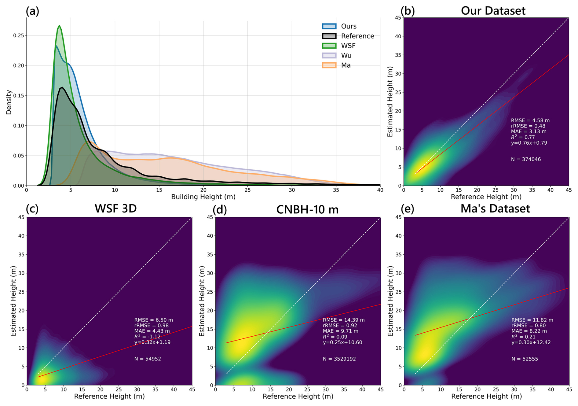
Figure 11 Comparsion of reference height, our dataset and other datasets in 2019. (a) Height distribution of different datasets; (b) Scatter plot of our dataset and reference heights; (c) Scatter plot of WSF 3D (Esch et al., 2022) and reference heights; (d) Scatter plot of CNBH-10 m (Wu et al., 2023) and reference heights; (e) Scatter plot of Ma's dataset (Ma et al., 2024a) and reference heights.

Our dataset achieves the best overall accuracy in Beijing in 2019 (Fig. 11b), with the lowest RMSE (4.58 m), rRMSE (0.48), and MAE (3.13 m), as well as a relatively high R² (0.77). CNBH-10 m, WSF 3D and Ma's datasets expose visible biases, with RMSE differing from 6.50 to 14.39 m and MAE differing from 4.43 to 9.71 m (Fig. 11c–e). Our dataset holds less underestimation compared to other datasets, while all these datasets express a tendency to underestimate the height of high-rise buildings. The annual distribution of building heights from 1990 to 2019 is shown in Fig. S3.

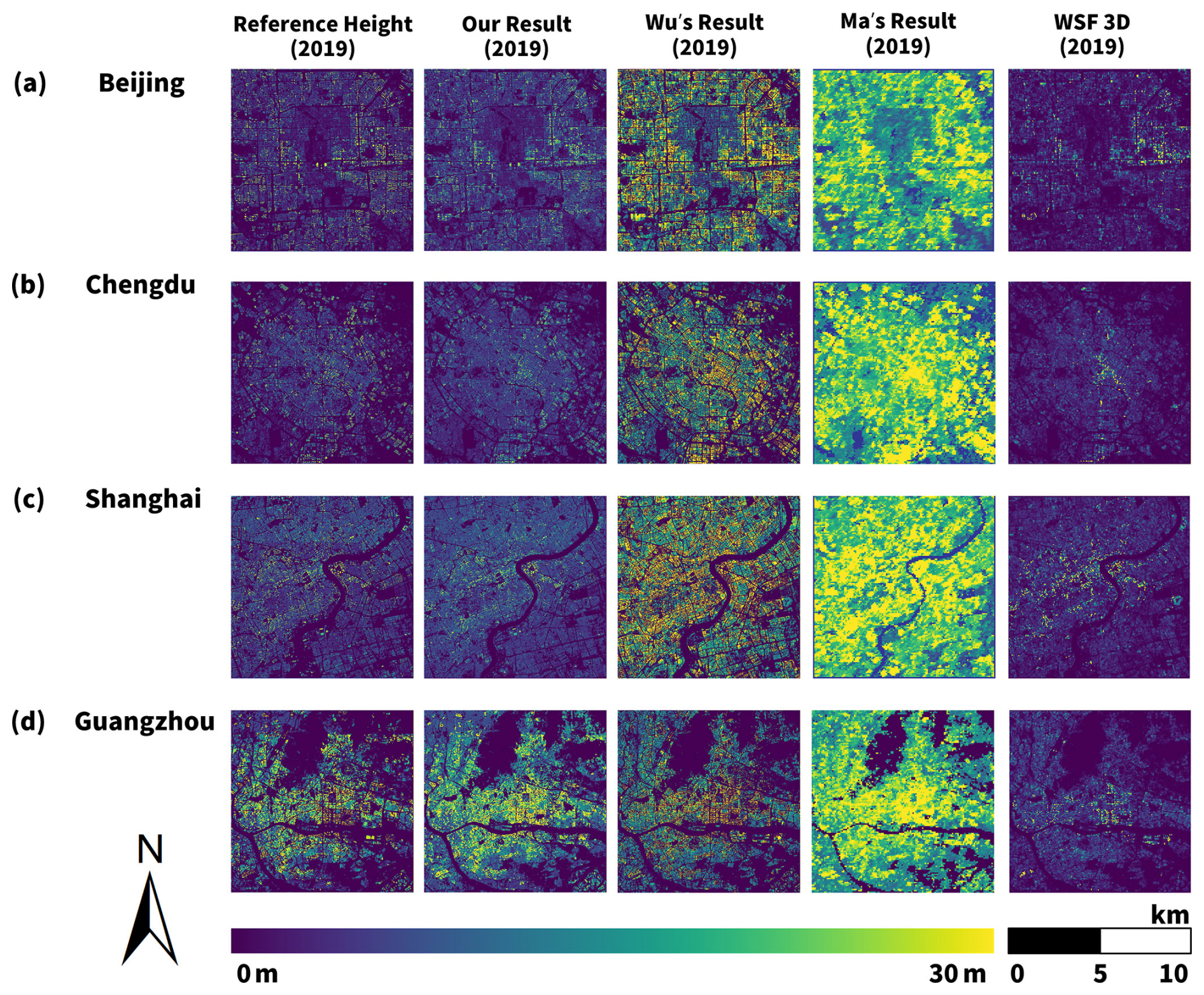
Figure 12 Comparison of building height datasets in different cities. (a) Beijing; (b) Chengdu; (c) Shanghai; (d) Guangzhou.

Visual comparisons across four major Chinese cities, namely Beijing, Shanghai, Chengdu, and Guangzhou, show that our dataset closely approximates the reference height distributions in all cities (Fig. 12). The Wu's and Ma's datasets systematically overestimate vertical structures in Beijing, Shanghai, and Chengdu, where building heights exhibit significant variability. In contrast, Guangzhou's predominantly high-rise urban morphology shows better alignment with Wu's and Ma's estimates, while WSF 3D underestimates heights. Our dataset successfully resolves this regional discrepancy, accurately capturing Guangzhou's high-density vertical urban growth alongside other cities' height heterogeneities.

4.4.2 Comparison with long-term building height products

To provide a comprehensive comparison with existing long-term building height products, three representative datasets are selected (Table 4): the 1985–2010 dataset of He et al. (2023), the 2005/2010/2015/2020 dataset of Chen et al. (2025), and the China Multi-Attribute Building (CMAB) dataset (Zhang et al., 2025a). Since He's dataset and CMAB record building construction completion years, the average building height for each reference year is calculated using buildings constructed before that year. For our dataset and Chen et al. (2025), direct annual height averaging is applied.

Table 4 Datasets selected for the long-term comparison.

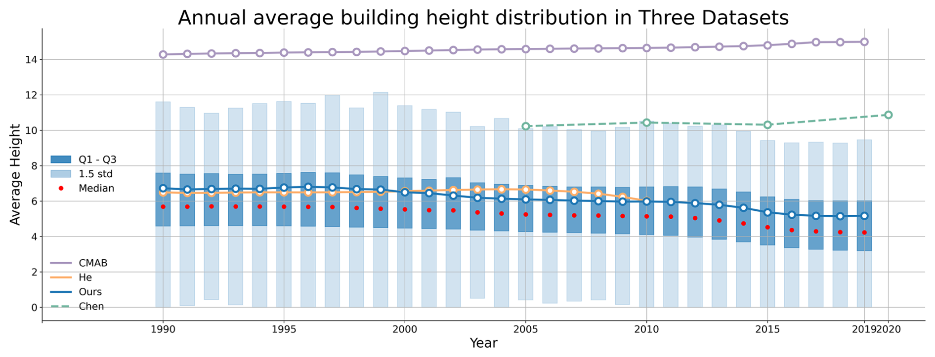
Figure 13 Temporal change in annual average height in three long-term building height datasets.

At the nationwide scale, Fig. 13 compares annual mean height trends across the four datasets. Median values, Q1/Q3 quartiles, and 1.5× standard deviation ranges comprehensively characterize height distributions. During 1990–2019, our dataset and He et al. (2023) show similar nationwide mean heights of approximately 5.17 and 5.18 m, respectively, whereas Chen et al. (2025) reports a higher mean height of approximately 10.44 m, and CMAB exceeds 14 m. These differences are mainly related to sample coverage and reference data sources. For example, CMAB focuses more on urban center built-up areas, while the other long-term datasets cover broader regions, including rural areas, townships, and low-density built-up areas. Despite these systematic height differences, all datasets show relatively stable temporal trends at the nationwide scale, suggesting that our dataset reasonably reflects the long-term stability of building height changes in China. The detailed value of annual mean height for our dataset is recorded in Table S5.

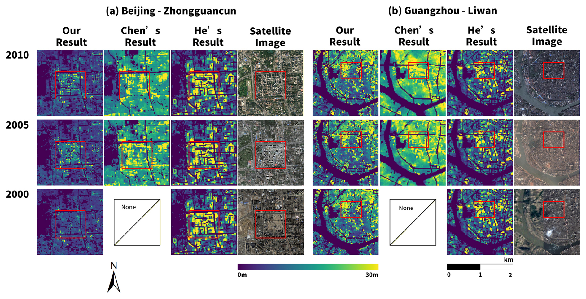
Figure 14 Comparison of long-term building height datasets in different cities. (a) Beijing; (b) Guangzhou. Satellite imagery is from © 2000, 2005, 2010 CNES/Airbus, Maxar Technologies, Google.

At the urban local scale, Beijing and Guangzhou are selected for detailed comparison. In Zhongguancun, Beijing, obvious urban renewal and demolition–reconstruction occur around 2005. He et al. (2023) does not sufficiently reflect the local redevelopment process, while Chen et al. (2025) shows temporal drifting with unreasonable height fluctuations for some stable buildings. Our dataset better reflects local building height growth and renewal (Fig. 14a). In Liwan District, Guangzhou, which has remained generally stable since 2005, Chen et al. (2025) also shows temporal drifting, whereas our dataset maintains better height continuity and temporal consistency (Fig. 14b).

4.4.3 Comparison with stable areas and historical imagery for temporal reliability validation

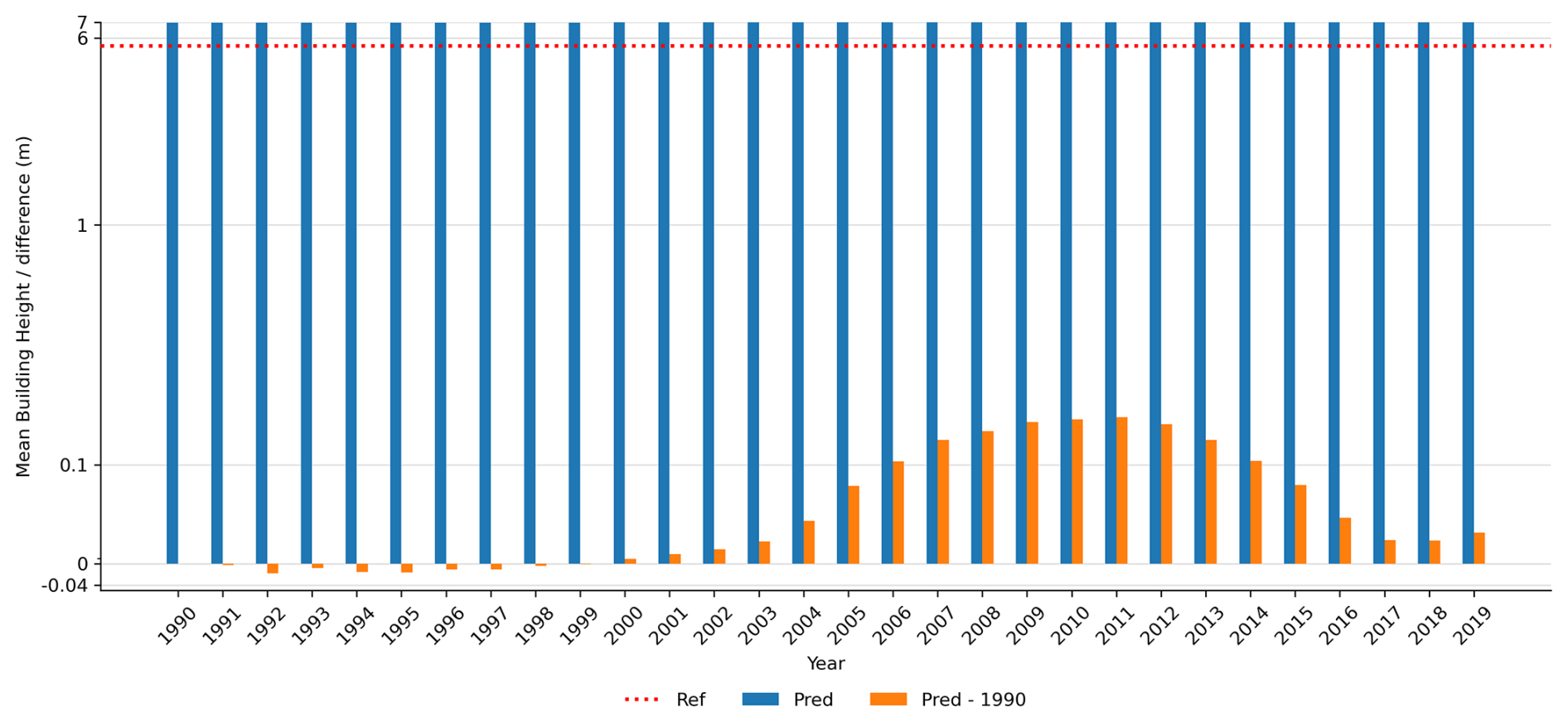
To evaluate the temporal stability of the generated building height dataset, stable areas are identified where building footprints and heights remain unchanged throughout the study period. These areas are defined as pixels with no change year detected by CCDC from 1990 to 2019. As shown in Fig. 15, the estimated mean building heights in these stable areas remain highly consistent over time. The highest mean height is 7.13 m in 2011, while the lowest is 6.95 m in 1992, corresponding to a fluctuation of less than 0.2 m. The mean reference height in 1990 is 5.58 m, shown by the red dotted line, and is close to the estimated heights. The orange bars show annual differences from the 1990 estimated height, with a maximum deviation of 0.17 m in 2011. These results indicate that the dataset does not introduce artificial temporal noise and maintains high temporal stability in areas without physical urban change.

Figure 15 Predicted height and reference height in stable areas.

To validate the reliability of the long-term building height dataset in building change areas, Figs. 16 and 17 examine three typical urban change contexts including persistent built-up, complete demolition, and new construction areas. For sampled cities, predicted heights are compared with reference heights and historical satellite imagery; for non-sampled cities, where reference height data are unavailable, historical satellite imagery is used as visual evidence for the extrapolated results.

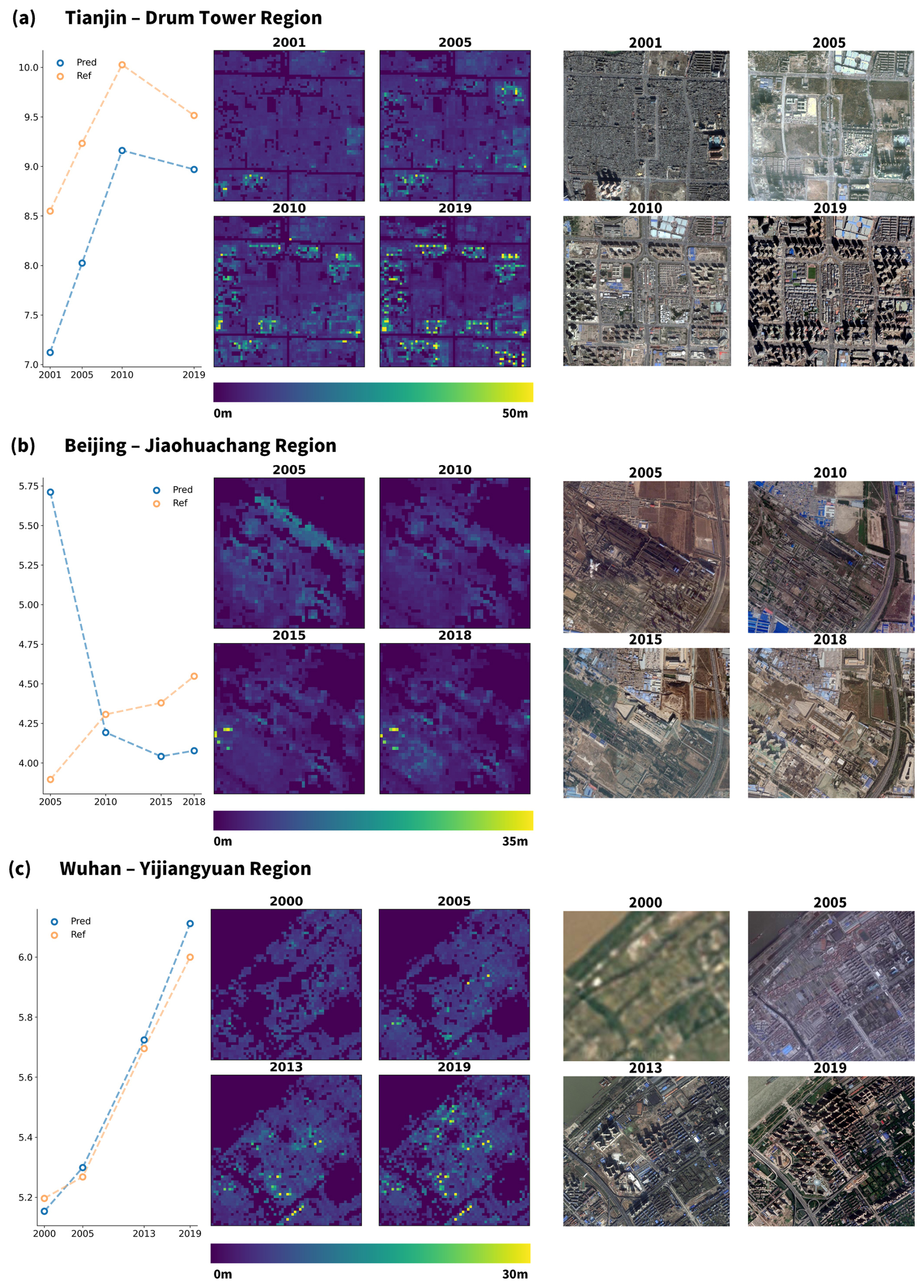
Figure 16 Comparison of urban areas in sampled cities using Google historical satellite imagery. (a) Drum Tower region, Tianjin; (b) Jiaohuachang region, Beijing; (c) Yijiangyuan region, Wuhan. Satellite imagery is from © 2000, 2001, 2005, 2010, 2013, 2015, 2018, 2019, CNES/Airbus, Maxar Technologies, Google.

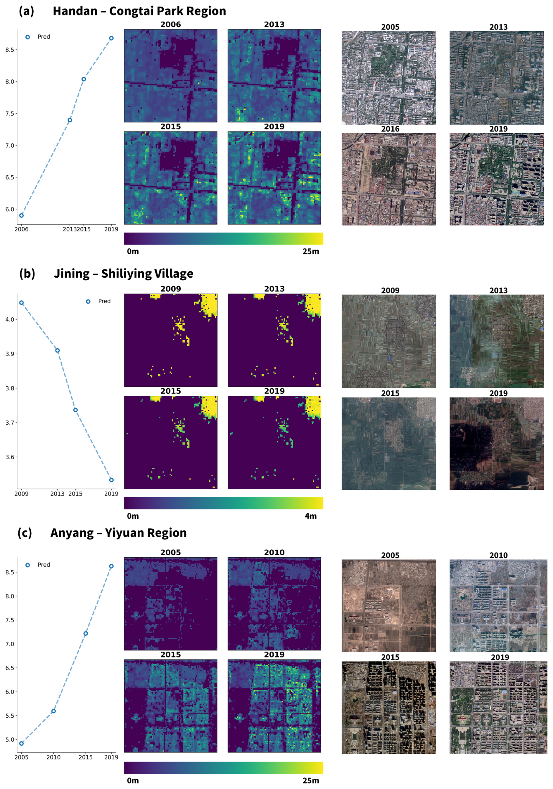
Figure 17 Comparison of urban areas in non-sampled cities using Google historical satellite imagery. (a) Congtai Park region, Handan; (b) Shiliying region, Jining; (c) Yiyuan region, Anyang. Satellite imagery is from © 2005, 2009, 2010, 2013, 2015, 2016, 2019 CNES/Airbus, Maxar Technologies, Google.

In sampled cities, the predicted heights generally agree well with both reference heights and historical imagery. For persistent built-up areas and new construction areas, such as Drum Tower in Tianjin (Fig. 16a) and Yijiangyuan in Wuhan (Fig. 16c), the dataset effectively captures building height dynamics. Taking Yijiangyuan as an example, the reference heights in 2000, 2005, 2013, and 2019 are 5.19, 5.26, 5.69, and 6.00 m, respectively, while the corresponding predicted heights are 5.15, 5.30, 5.72, and 6.11 m, with errors all below 0.11 m. For the complete demolition case, Jiaohuachang in Beijing (Fig. 16b) is selected. The estimated height decreases from 5.71 to 4.04 m, consistent with the demolition and redevelopment process visible in historical imagery. As described in Sect. 3.1.1, annual reference heights are derived from persistent built-up areas identified using the 2019 reference data and CCDC breakpoint information, rather than direct observations of all historical building pixels. Therefore, the 2005 difference between the predicted and reference heights, 5.71 m versus 3.52 m, mainly arises from the applicability limitation of the annual reference data generation method in demolition areas. This difference reflects the limited representativeness of the reference height for demolished buildings, rather than model bias or a data error in the generated dataset.

In non-sampled cities, mapped temporal trends are broadly consistent with visually identifiable urban changes. The estimated height at Handan Congtai Park (Fig. 17a) increases from 5.90 to 7.40, 8.04, and 8.68 m, reflecting redevelopment from bungalows to multi-story apartments. At Jining Shiliying Village (Fig. 17b), the estimated height decreases from 4.05 to 3.91, 3.74, and 3.53 m, consistent with settlement abandonment and demolition caused by subsidence. For Anyang Yiyuan (Fig. 17c), the estimated height increases from 4.91 to 5.60, 7.22, and 8.63 m, reflecting progressive new construction on previously undeveloped land. These results indicate that the generated dataset can reasonably characterize long-term building height dynamics across persistent built-up, demolition, and new construction areas.

4.5 Mapping of annual Chinese building heights

4.5.1 Dynamic of building height

As the start and end years of our dataset, 1990 and 2019 are selected to illustrate China's building height distributions (Fig. 18a, b). Given the large data volume, visualizations are aggregated to 1 km resolution for national-scale representation. During this period, urban built-up areas expanded substantially, accompanied by a clear increase in building heights. This trend is most pronounced on the North China Plain and in fast-growing metropolitan regions of central and eastern China.

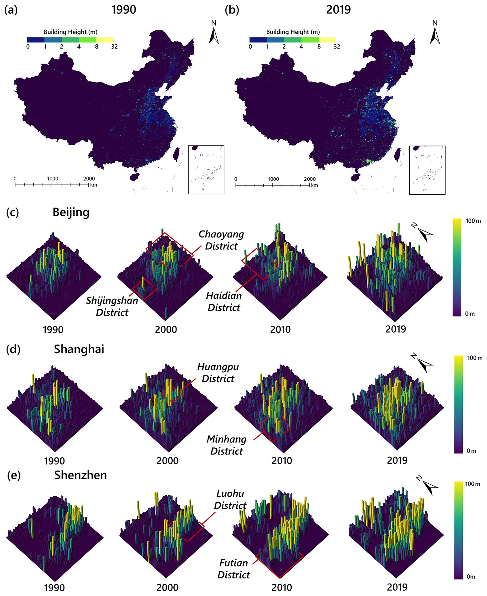
Figure 18 Spatial distribution and temporal progression of building heights. (a, b) Spatial distribution of building heights in 1990 and 2019; (c–e) Temporal progression of building height in Beijing, Shanghai and Shenzhen.

City-level temporal visualizations for Shanghai, Beijing and Shenzhen (Fig. 18c–e) depict their urbanization trajectories in 1990, 2000, 2010, and 2019. Core urban areas maintain relatively stable building heights, with only incremental additions of high-rise structures in all three cities. Peripheral districts undergo rapid land conversion and construction, resulting in taller and denser building clusters over time. For example, in Shenzhen, Luohu District had the tallest skyline in 1990, while Futian District experienced concentrated development after 2000, eventually surpassing Luohu in building height and density.

4.5.2 Dynamic of building volume

Our dataset presents a consistent depiction of both horizontal and vertical expansion of the built environment across China from 1990 to 2019, accurately capturing nationwide urban building growth over the past three decades. During this period, total building volume increased markedly from 365.98 km³ in 1990 to 882.43 km³ in 2019, while total impervious surface area expanded from 54 407.03 to 170 595.06 km².

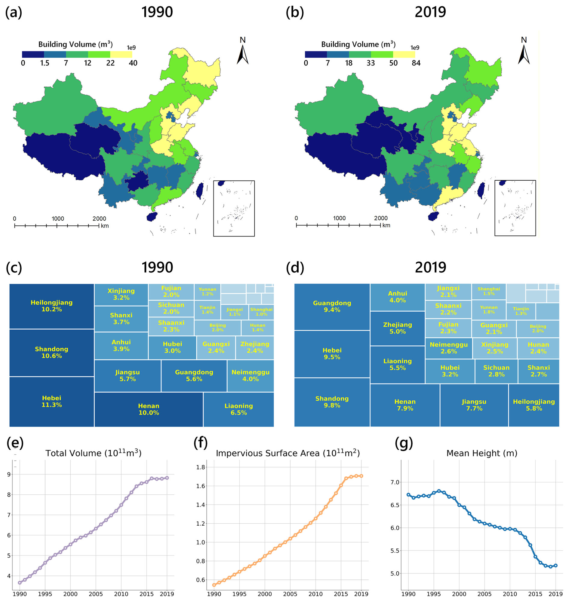
Figure 19 Spatial distribution and temporal progression of building volume, impervious surface area and mean building height. (a, b) Spatial distribution of building volume in 1990 and 2019; (c, d) Share of building volume of each province of China; (e–g) Temporal progression of building volume, impervious surface area and mean building height.

Figure 19a and b illustrate widespread volumetric growth across almost all provinces, despite the pronounced regional heterogeneity. By 2019, national building volume reaches approximately 882.43 km³, which is generally consistent with GlobalBuildingAtlas estimates (approximately 700 km³; Zhu et al., 2025). At the city scale, our estimates display strong agreement with 3D-GloBFP (Che et al., 2024), such as Beijing (ours: 17.0 km³ vs. 13 km³) and Shanghai (ours: 12.7 km³ vs. 14.1 km³).

Figure 19c and d further show shifting contributions to national building volume. In 1990, Hebei (11.3 %), Shandong (10.6 %), and Heilongjiang (10.2 %) were the largest contributors. By 2019, Shandong becomes the highest (9.8 %), while coastal provinces such as Guangdong (9.4 %) and Jiangsu (7.7 %) gain substantially in their share, indicating accelerated coastal urbanization driven by economic growth.

Figure 19e–g show the temporal evolution of total building volume, impervious surface area, and mean building height, respectively. Although the mean building height exhibits a slight declining trend after 1990, indicating that outward expansion slightly outpaces vertical increase, both building volume and impervious surface area continue to increase. The growth rate of building volume begins to slow around 2016 and approaches a relatively stable level by 2019. For impervious surface area, a decline in growth rate occurs after 2016, with subsequent increases remaining relatively modest. Annual values for these indicators are provided in Table S5.

4.6 Uncertainty analysis and limitations

Although the generated long-term building height dataset shows good overall accuracy and temporal consistency, several limitations and uncertainty sources should still be considered to support appropriate data use. Spatial uncertainty varies across regions because the reliability of building height mapping depends on the similarity between predicted pixels and the training samples in the feature space. Areas whose feature distributions deviate from the training samples may have higher uncertainty. This sample-representation issue is also reflected in some high-rise areas, where underestimation remains mainly due to the limited availability of high-rise reference samples.

In addition to feature-space similarity, uncertainty in the building height mapping may also arise from reconstructed VV, CCDC-based change detections, and the use of geographic coordinates as spatial predictors. First, the joint use of reconstructed VV with spectral and topographic variables suppresses random reconstruction noise during height estimation. Although localized inaccuracies may appear as discrete low-confidence areas in heterogeneous landscapes, they do not distort the overall spatial patterns of the final 30 m building height maps. Second, uncertainty may be higher in the early period because of the relative sparsity of CCDC-based change detections and the constrained availability of historical Landsat observations during the 1990s, which result in lower transfer accuracy of reference data. The pre-2000 estimates still demonstrate high reliability in capturing regional-scale urban expansion, provincial building volume trends, and metropolitan-level development trajectories, although caution is advised when conducting fine-grained, pixel-level, year-to-year causal interpretations. Third, geographic coordinates help capture regional spatial trends and broad-scale variations in urban morphology, but may also introduce risks of spatial overfitting. The training dataset covers most of China's topographical and climatic regions, allowing the models to capture the major patterns of urban morphology. Spatial transferability remains limited for cities excluded from the reference samples, especially where local zoning or building morphology differs substantially from the training data.

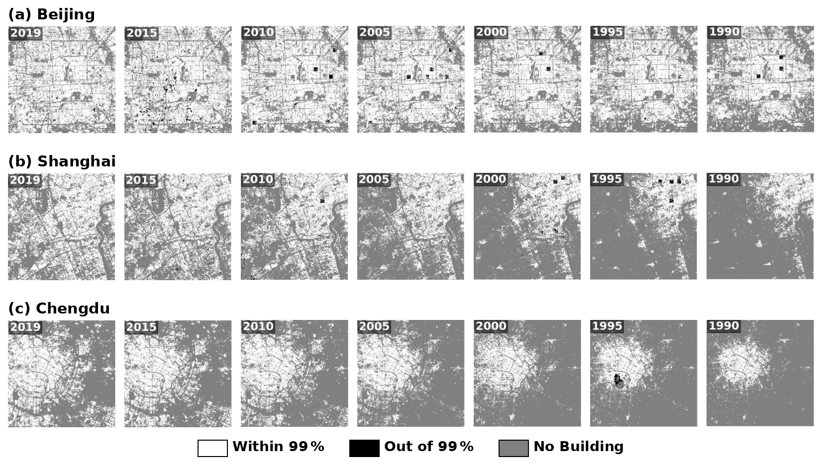
Figure 20 Binary confidence layers for three representative cities. (a) Beijing; (b) Shanghai; (c) Chengdu.

To provide additional reliability information, a per-pixel confidence layer is generated using the Mahalanobis distance (MD), which measures the distance between each predicted pixel and the multivariate distribution of the training samples (Lee et al., 2018):

$$\begin{array}{}\text{(12)}& D_{\mathrm{M}}\left(\mathit{x}\right)=\sqrt{{\left(\mathit{x}-\mathit{\mu }\right)}^T{\mathbf{\Sigma }}^{-\mathrm{1}}(\mathit{x}-\mathit{\mu })}\end{array}$$

where D_M(x) denotes the Mahalanobis distance of a pixel's value vector x, μ is the mean vector of the training samples, and Σ⁻¹ is the inverse matrix. A lower MD value indicates that the pixel is closer to the training sample distribution and has higher confidence, whereas a higher MD value indicates greater uncertainty.

For easier interpretation, $D_{\mathrm{M}}^{\mathrm{2}}$ is converted into a 0–1 confidence score using the survival function of the χ² distribution. A threshold of α=0.01 is then used to generate a binary confidence layer, where pixels within the 99 % confidence range are regarded as reliable, while pixels outside this range are considered potential outliers or extrapolated samples and should be used with caution (Etherington, 2019; Frost, 2020).

The binary confidence layer is further examined in representative cities, including Beijing, Shanghai, and Chengdu (Fig. 20). From 1990 to 2019, most building areas in these cities fall within the 99 % confidence range, indicating that their feature distributions are generally close to the training samples and that the corresponding estimates are reliable. Beijing and Shanghai show good spatial continuity across all selected years, with only sparsely distributed low-confidence patches. Chengdu also shows a high proportion of reliable building areas in most years, although a relatively concentrated low-confidence area appears in 1995, possibly related to early built-up extent, remote sensing feature quality, or local morphology differences. These results demonstrate the reliability of the dataset across representative Chinese cities. Remaining uncertainties suggest that further refinement could be beneficial for improving the dataset across different urban contexts.

5 Data availability

Data described in this manuscript can be accessed at https://doi.org/10.6084/m9.figshare.29918978 (Zhang et al., 2025b). The dataset is stored in TIF format. Each image covers a 2° × 2° area, with its name representing the lower left longitude and latitude of the region. Each image has 30 bands, from the first band storing building height data of 2019, to the last band of 1990.

6 Conclusion and future work

The first long-term, continuous annual building height dataset for China from 1990 to 2019 at 30 m resolution is established through the integration of multi-source and multi-temporal remote sensing data with machine learning. By reconstructing SAR backscatter, applying CCDC-based reference data, and incorporating TV denoising, the dataset maintains year-to-year consistency and captures inter-annual variations in building heights. Accuracy assessments indicate high precision and stable performance over three decades, with RMSE ranging from 3.20 to 4.27 m, MAE from 2.27 to 2.95 m, and R² between 0.76 and 0.82, despite the reduced availability of high-resolution variables in earlier years. In addition, our dataset demonstrates higher accuracy in Beijing for 2019 compared to that of Wu et al. (2023), reducing the RMSE from 14.39 to 4.58 m. Validation against existing building height products and historical satellite imagery further demonstrates its reliability and generalizability, ensuring broad applicability for both national and localized urban morphology analyses. Moreover, our dataset reveals that both built-up area and building volume continue to expand nationwide from 1990 to 2019. Meanwhile, the contributions of different provinces to the national building volume vary considerably over time, reflecting heterogeneous urban development trajectories across regions.

For future dataset updates, incorporating multi-source training data, such as airborne LiDAR observations, could be beneficial. LiDAR data provide more direct and accurate height measurements, which may help alleviate current limitations in spatial generalization and reduce the underestimation of high-rise buildings, thereby further improving model robustness in complex urban environments (Chen et al., 2025; Ma et al., 2024a). Beyond improving the accuracy of historical mapping, subsequent dataset updates should also consider the prospective trajectories of urban growth in the coming decades. As land resources become increasingly constrained and population increases, the developmental paradigm shifts from increment to stock (Frolking et al., 2024; Koziatek et al., 2016). Future trajectories are likely to involve more intensive use of vertical space within relatively stable built-up footprints. Under this scenario, the mean building height of built-up areas continues to rise, marking a transition from land-extensive growth to space-efficient densification. Extending the current framework to construct forward-looking datasets that project such trajectories represents a critical direction, offering opportunities to anticipate future morphological change and support urban sustainability planning.