SEAS5-BCSD: a bias-corrected and downscaled global seasonal forecast reference dataset for 1981–2024

Seasonal forecasts offer valuable information on upcoming conditions for the water, energy, and agricultural sectors. However, applications of raw data from global seasonal forecasts are limited, as they can show substantial biases and temporal drifts. In this study, we present a bias-corrected and downscaled global seasonal forecast reference dataset for precipitation and 2 m temperature for 1981 until 2024, provided at monthly resolution. We achieve this with the Bias Correction and Spatial Disaggregation (BCSD) method, combining ECMWF SEAS5 seasonal forecasts with ERA5 reanalysis data. The resulting post-processed product is a spatially refined and improved dataset for a wide range of seasonal applications in the water, energy and agricultural sectors. Unlike existing products, the dataset provides bias-corrected forecasts for all SEAS5 ensemble members over the full hindcast period (1981–2016) and even beyond (until 2024). The dataset spans all global land areas at 0.25° spatial resolution with a forecast lead time of up to seven months. It comprises 25 ensemble members for the period 1981–2016 and 51 ensemble members for 2017–2024. To assess probabilistic forecast quality, we conduct a comprehensive performance evaluation, using the Brier Skill Score (BSS) and the Continuous Ranked Probability Skill Score (CRPSS). The BCSD-corrected temperature forecasts outperform climatology across nearly all regions and lead times, with highest skill in flat and warm regions. Precipitation skill is highest in the tropics and humid regions. Semi-arid areas show solid skill during the rainy season but reduced performance in dry months. This skillful global seasonal forecast reference dataset can now be explored by the community for subsequent forecast evaluation, drought prediction studies, and water resource management applications. The BCSD-corrected seasonal forecast dataset is publicly available as NetCDF data under a Creative Commons Attribution 4.0 International License (CC BY 4.0) at the World Data Center for Climate (WDCC; https://doi.org/10.26050/WDCC/SEAS5-BCSD, Weber et al., 2026).

1 Introduction

Droughts, prolonged heat waves, heavy rainfall, and large-scale floods: recent years have shown that improved adaptation to hydrometeorological extremes needs to be achieved in many regions worldwide. These extreme events occur with increasing frequency and intensity due to climate change (Di Capua and Rahmstorf, 2023). Among them, droughts pose a particularly severe threat to society due to their extensive spatial scale and prolonged duration compared to floods (United Nations Convention to Combat Desertification, 2022).

Knowledge of hydrometeorological wet/dry or hot/cold anomalies months ahead allows improved preparedness for stakeholders, such as water managers and large-scale farmers, to mitigate the impacts of extreme periods. While floods are often associated with short warning times of hours to days due to their high spatial complexity (Cloke and Pappenberger, 2009), droughts and heatwaves need to be predicted well over a month in advance due to their large-scale and long-term nature. Extended predictability allows stakeholders to implement effective countermeasures, which can be scaled according to the predicted severity of the event (Portele et al., 2021).

Seasonal forecasts provide valuable insights into upcoming conditions, offering a forecast horizon of up to twelve months. The drivers of predictability in seasonal forecasting systems are primarily twofold. The initial atmospheric state at the beginning of the simulation plays a key role in the first few weeks of the forecast, as it contains essential information about circulation patterns. For longer forecast durations, predictability is largely governed by teleconnections, which are primarily influenced by sea surface temperature (SST) variations (Materia et al., 2014). Despite these sources of skill, the inherently chaotic nature of the atmosphere limits the accuracy of forecasts several months in advance (e.g. Vitart et al., 2017). Multiple national and international meteorological services, including the German Weather Service (DWD), the UK Met Office, the Australian Bureau of Meteorology, and the European Centre for Medium-Range Weather Forecasts (ECMWF), operate seasonal forecasting systems (e.g. Fröhlich et al., 2021; Johnson et al., 2019; Hudson et al., 2017; MacLachlan et al., 2014), openly available via the Copernicus Data Store. However, the raw output of these models often lacks realism in terms of magnitude and variability (Yin et al., 2023, Fig. 1), making it unsuitable for direct application in downstream models such as hydrological or agricultural simulations. To address this, a range of bias correction methods have been developed and applied to seasonal forecast datasets, resulting in a combination of reference and model data. Global bias-corrected seasonal forecast datasets remain scarce, and only a limited number of products have been described in the literature. Existing examples include the long-range component of the MSWX product (Beck et al., 2022), as well as several regional (Lorenz et al., 2021; Ballarin et al., 2023) or application-specific datasets (Geiger et al., 2024). However, many existing products focus on particular regions or variables, provide only a subset of ensemble members, or are based on climate projections rather than operational seasonal forecasts. Consequently, comprehensive global archives combining high spatial resolution, long temporal coverage, and large ensemble sizes remain rare.

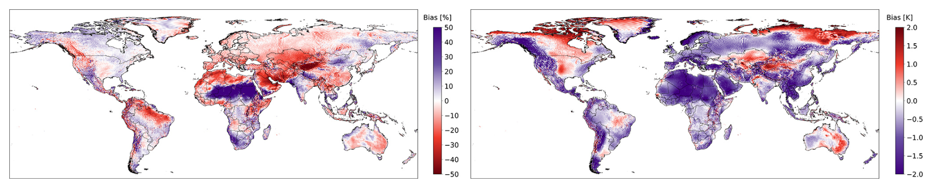
Figure 1 Mean bias of uncorrected SEAS5 (“raw”) forecasts Lead Month 1 relative to ERA5 for precipitation (left) and temperature (right) for the reference period (1981–2016). Precipitation bias is shown as relative deviation (%), and temperature bias as absolute deviation (K).

Extreme climatic conditions, such as severe large-scale droughts, are inherently difficult to capture due to their rare occurrence. In many cases, only a small fraction of ensemble members represent such extremes. Therefore, robust probabilistic assessment of climate risks requires access to the full ensemble distribution. We provide bias-corrected forecasts for all 25 ensemble members of the high-resolution (36 km) SEAS5 system, covering the period from 1981 to 2016 and all 51 ensemble members from 2017 onward. Rather than serving as a competing product, this reference dataset is intended to complement existing products and to support a broader range of applications and analyses. While numerous studies have evaluated forecast skill at regional scales (e.g. Crespi et al., 2021; Wang et al., 2019), comprehensive global analysis of bias corrected seasonal forecasts is still sparse. This study aims to close this gap by presenting a bias-corrected global seasonal forecast dataset based on ECMWF's SEAS5 system, designed to serve as a reference dataset. In addition, we provide a detailed global assessment of the dataset's strengths and limitations using a suite of established forecast evaluation metrics.

2 Methods

2.1 Data

Our dataset is based on the high-resolution version of the SEAS5 Seasonal Forecasting System of the European Centre for Medium-Range Weather Forecasts (ECMWF). SEAS5 provides global coverage at approximately 36 km resolution, with daily timesteps and 91 atmospheric layers (Johnson et al., 2019). The forecast horizon lies at 215 d. SEAS5 is released on the 5th day of each month, minimizing the gap between the start of a new month and the availability of a new forecast.

SEAS5 offers a wide range of variables, of which we focus on total precipitation (tp) and mean 2 m air temperature (t2m). A key advantage of SEAS5 is the availability of historical reforecasts for 1981–2016, which allows the construction of cumulative distribution functions (CDFs) for statistical bias correction using an extensive data pool. This enhances the detection of extreme events by expanding the range of possible outcomes (this point will be discussed in detail later in the context of the BCSD method). Additionally, to complement the analysis of drought conditions, the one-month Standardized Precipitation Evapotranspiration Index (SPEI-1) is computed following the approach of Vicente-Serrano et al. (2010).

For the analysis in this article, we use the 1981–2016 hindcast period with cross validation. SEAS5 re-forecasts during this period are produced with 25 ensemble members, whereas the operational forecast system generates 51 members for real-time forecasts; including the operational period in the statistical analysis would therefore introduce an inhomogeneity in ensemble size (Johnson et al., 2019). Reducing the operational ensemble to 25 members to match the hindcast set is not advisable due to the chaotic nature of the stochastic perturbations in SEAS5 and the potential loss of valuable spread information inherent to the system. Using only the consistent hindcast ensemble ensures that skill metrics reflect the forecast system's performance and not changes in ensemble sampling characteristics.

Bias-correction cumulative distribution functions (CDFs) are therefore derived exclusively from the consistent 1981–2016 hindcast dataset and subsequently applied unchanged to the 2017–2024 operational forecasts. This fixed calibration strategy ensures a temporally homogeneous framework and avoids distortions in the estimated forecast distributions caused by the differing ensemble sizes. Alternative approaches, such as incorporating all available operational ensemble members into the calibration or selecting a reduced subset of operational members, were not applied. Including all operational members would disproportionately weight the 2017–2024 period in the empirical distributions, while sub-sampling introduces additional methodological degrees of freedom related to ensemble representativeness and spread preservation. The adopted approach is consistent with standard bias-correction practice in seasonal forecasting, where calibration is typically performed on a fixed reforecast (hindcast) period and subsequently transferred to operational forecasts. Restricting the calibration to the hindcast period therefore provides the most consistent framework for evaluating forecast skill and applying bias correction.

As a reference product, we selected ECMWF's ERA5 reanalysis. ERA5 covers the period from 1940 to three days before the current date, fully encompassing both the reference and validation periods. It has a spatial resolution of 0.25°×0.25° and an hourly temporal resolution. ERA5 has been proven to be one of the most reliable global reanalysis datasets, covering all required variables for our study (Hersbach et al., 2020). It has been extensively validated for selected variables (e.g. Lavers et al., 2022), for global applications (Nogueira, 2020) regional studies (Bandhauer et al., 2021), etc. That being said, we are well aware that ERA5 has its limitations (see Sect. 4.2). Nevertheless, being one of the most commonly used global references for precipitation and temperature, we are convinced, that ERA5 is an appropriate and representative reference for evaluating the forecast skill of the SEAS5-BCSD dataset. To ensure comparability with SEAS5, ERA5 data are aggregated to daily sums or means, respectively. We refrained from using ERA5-Land due to its delayed availability, typically two to three months after the release of the standard ERA5 dataset. Additionally, ERA5 offers the same set of ground-level variables as SEAS5, facilitating direct comparison.

2.2 Bias correction and spatial disaggregation

Several studies (e.g. Weber et al., 2023; Lorenz et al., 2021; Portele et al., 2021) highlight the limitations of uncorrected SEAS5 data and emphasize the necessity of bias correction. Lorenz et al. (2021) demonstrated significant performance improvements for semi-arid regions when applying a statistical bias correction. Building on this, Portele et al. (2021) demonstrated across seven drought-prone regions worldwide that using normalized seasonal forecasts can yield substantial economic benefits, including a real-world case in which approximately USD 16 million in potential losses at a hydropower reservoir in Sudan could have been avoided. Using a similar statistical correction approach, Weber et al. (2023) identified forecast skill over Germany, a region with a more complex seasonal climate (Doblas-Reyes et al., 2013b) and thus more challenging predictability than semi-arid regions. These findings motivated us to develop a global bias correction approach. The primary challenge is to design a computationally efficient method that provides bias-corrected forecasts within hours of downloading the raw SEAS5 data, ensuring the timely availability of the valuable first lead month.

For statistical bias correction of original and raw SEAS5, we here employ the Bias Correction and Spatial Disaggregation (BCSD, Wood et al., 2004) method to generate the new dataset SEAS5-BCSD. The resulting dataset is therefore not a redistribution of SEAS5 model output but a statistically post-processed reference product that combines information from both SEAS5 forecasts and ERA5 reanalysis data. BCSD consists of two main components: (i) a bias correction step that applies quantile-quantile mapping to harmonize the forecast with the reference dataset and (ii) a spatial downscaling step to refine the resolution of the bias-corrected data.

We modified the sequence of Bias Correction (BC) and Spatial Disaggregation (SD) following the methodology outlined in Lorenz et al. (2021) for avoiding numerical issues. In this approach, spatial disaggregation from the coarse SEAS5 grid to the higher-resolved ERA5-Land grid is performed using bilinear interpolation applied directly to the forecast variables (precipitation and temperature), rather than to anomaly fields. After interpolation, a post-processing quality control step is applied to remove physically implausible values like negative precipitation. Bias correction is subsequently applied on each forecast day using Empirical Quantile Mapping (EQM), which is suited for precipitation extremes (Golian and Murphy, 2022). A more detailed discussion of the advantages and limitations of EQM is provided in Sect. 4.2. This method constructs a cumulative distribution function (CDF) for each pixel separately for both the reference dataset and the seasonal forecast over the reference period. Each daily CDF is based on all corresponding days from the 36-year reference period and hence an empirical distribution following Boé et al. (2007). To smooth the CDF, a fixed-width time window of 15 d centered on the target date is utilized, incorporating values from preceding and succeeding days. This approach helps to capture more extreme events. Consequently, the CDF becomes better resolved and extended at both its upper and lower ends. However, if the time window is too large, it may incorporate data from the wrong season, introducing an own bias when correcting the target date. Near the beginning and end of the forecast horizon, the time window is truncated according to the availability of SEAS5 data, and the corresponding days are selected from ERA5. This contrasts with the approach of Lorenz et al. (2021), where the ERA5 window was not truncated to match the length of the SEAS5 forecasts. Overall, each daily ERA5 CDF is constructed from 1116 data points per grid cell. For SEAS5, the inclusion of ensemble members expands the dataset to a total of 27 900 values per forecast day. Due to seasonal forecast drifts varying by issue month, SEAS5 CDFs are computed individually for each issue months 215 d.

Applying bias correction on a global scale presents computational challenges, particularly concerning processing time. To accelerate calculations, the CDFs are precomputed and stored rather than generated dynamically. While this significantly enhances computational efficiency, it necessitates substantial storage capacity. To manage storage requirements, the CDFs are downsampled to 200 data points, reducing the total storage footprint significantly.

For bias correction of new forecasts, each forecasted value is first mapped onto the SEAS5 CDF to determine its probability. This probability is then used to obtain the corrected value by mapping it onto the ERA5 CDF. However, if a forecasted value exceeds the historical maximum or falls below the historical minimum, the CDF approach alone is insufficient due to the absence of a corresponding probability. Several methods exist to address this issue, including fitting a statistical distribution such as the Generalized Pareto Distribution (Volosciuk et al., 2017) or applying linear extrapolation (Gonzalez-Aparicio and Hidalgo, 2011; Holthuijzen et al., 2022). In this study, precipitation extremes are treated using a linear extrapolation (scaling) approach, while temperature extremes are corrected using an additive delta approach following Boé et al. (2007). Let F⁻¹(p) denote the empirical quantile function of the reference cumulative distribution function (CDF). If a forecast value x exceeds the empirical range, it is mapped to the nearest available boundary quantile $x_{\text{ref}}=F^{-\mathrm{1}}\left(p_{max}\right)$ (or $F^{-\mathrm{1}}\left(p_{min}\right)$ for lower extremes).

For precipitation, a scaling factor is defined as

$$\begin{array}{}\text{(1)}& {\displaystyle }{\displaystyle }s={\displaystyle \frac{x}{x_{\text{ref}}}},\end{array}$$

and applied such that the corrected value becomes

$$\begin{array}{}\text{(2)}& {\displaystyle }{\displaystyle }{x}^{*}=s\cdot F^{-\mathrm{1}}\left(p\right),\end{array}$$

thereby preserving the relative deviation from the reference distribution.

For temperature, an additive offset is computed as

$$\begin{array}{}\text{(3)}& {\displaystyle }{\displaystyle }\mathrm{\Delta }=x-x_{\text{ref}},\end{array}$$

and applied as

$$\begin{array}{}\text{(4)}& {\displaystyle }{\displaystyle }{x}^{*}=F^{-\mathrm{1}}\left(p\right)+\mathrm{\Delta },\end{array}$$

which shifts the reference distribution by the same anomaly observed at the boundary.

Additionally, special handling is required for cases where precipitation values reach 0 mm in either the ERA5 or SEAS5 CDFs. Let $p_{\text{dry}}^{\text{ERA5}}$ and $p_{\text{dry}}^{\text{SEAS5}}$ denote the dry-day probabilities in the respective distributions.

If $p_{\text{dry}}^{\text{ERA5}}>p_{\text{dry}}^{\text{SEAS5}}$, all forecast values below the ERA5 dry-day threshold

$$\begin{array}{}\text{(5)}& {\displaystyle }{\displaystyle }x\le F_{\text{SEAS5}}^{-\mathrm{1}}\left(p_{\text{dry}}^{\text{ERA5}}\right)\end{array}$$

are set to 0 mm, ensuring consistency in dry-day frequency.

Conversely, if $p_{\text{dry}}^{\text{SEAS5}}>p_{\text{dry}}^{\text{ERA5}}$, additional dry days are introduced by stochastic sampling. For each forecasted zero value in SEAS5, a value is drawn from the truncated ERA5 distribution conditioned on precipitation below the dry-day threshold:

$$\begin{array}{}\text{(6)}& {\displaystyle }{\displaystyle }x\sim F_{\text{ERA5}}\left(x\mid x\le F_{\text{ERA5}}^{-\mathrm{1}}\left(p_{\text{dry}}^{\text{SEAS5}}\right)\right).\end{array}$$

Accurate daily forecasts over extended lead times exceeding two hundred days are not realistic due to inherent limitations in predictability (Krishnamurthy, 2019). Therefore, forecasts were aggregated to a monthly resolution to enhance robustness and interpretability. In the following, the aggregated time steps are referred to as “Lead Month” 0 through 7, with the initialization month denoted as the “issue month”. Lead Month 0 comprises forecast days 1–30 (depending on the respective calendar month), representing one month into the future. Although the bias correction method is applied globally across all grid cells, oceanic regions and Antarctica were subsequently masked out due to their limited relevance for most land-based hydrological and agricultural applications.

2.3 Continuous Ranked Probability Skill Score (CRPSS)

To estimate forecast skill, we employ various performance metrics to capture a plethora of characteristics of the bias-corrected forecasts. It should be noted that improvements due to bias correction depend on the verification metric, as distributional adjustments do not necessarily translate monotonically into changes in all categorical skill scores (Manrique-Suñén et al., 2020).

The evaluation of forecast accuracy can be conducted using the Continuous Ranked Probability Score (CRPS), following Hersbach (2000). For each pixel and each time step, the CRPS quantifies the deviation of forecasted values from the observed values, in this case, the ERA5 reanalysis dataset. Due to the probabilistic nature of SEAS5 forecasts, a simple coefficient of determination (R²) is insufficient, as it does not account for ensemble members. Instead, the CRPS is used, defined as:

$$\begin{array}{}\text{(7)}& {\displaystyle }{\displaystyle }\text{CRPS}(F,x)=\underset{-\mathrm{\infty }}{\overset{\mathrm{\infty }}{\int }}{\left(F\left(y\right)-H(y-x)\right)}^{\mathrm{2}}\mathrm{d}y,\end{array}$$

where H(y−x) is the Heaviside step function, F(y) represents the cumulative distribution function (CDF) of the probabilistic forecast values, and x is the observed value. The CRPS thus quantifies the area between the Heaviside function, which transitions from 0 to 1 at the observed value, and the forecast CDF. This computation is performed individually for each pixel and each time step. The CRPS values range from 0 to ∞, where a value of 0 indicates a perfect forecast.

To facilitate the comparison of CRPS values across different forecasting approaches, the Continuous Ranked Probability Skill Score (CRPSS) is utilized:

$$\begin{array}{}\text{(8)}& {\displaystyle }{\displaystyle }\text{CRPSS}=\mathrm{1}-{\displaystyle \frac{{\text{CRPS}}_{\text{fcst}}}{{\text{CRPS}}_{\text{ref}}}}.\end{array}$$

Here, CRPS_fcst is the CRPS of the forecast under evaluation, while CRPS_ref refers to the CRPS of a reference dataset, such as a climatology derived from a reanalysis dataset like ERA5 or an alternative forecast (e.g. uncorrected data). The CRPSS ranges from 1 to −∞, where a value of 1 represents a perfect forecast, 0 signifies performance equivalent to the reference, and negative values indicate performance worse than climatology. However, in a probabilistic forecasting system like SEAS5, achieving a CRPSS of 1 is not possible, as ensemble spread is a desirable feature. Maintaining the SEAS5 ensemble spread results in a maximum achievable CRPSS of approximately 0.6–0.8 for precipitation, depending on the region.

2.4 Brier Skill Score (BSS)

In addition, the Brier score is applied to the data. The score, introduced by Brier (1950), can be focused on a specific event, e.g. a forecast of precipitation lower than the 33rd percentile. Therefore, the Brier Score is useful for the evaluation of commonly used probability-based forecast maps such as tercile maps and is also suitable for assessing the performance of extreme forecasts. We calculate the Brier Score following Brier (1950) as

$$\begin{array}{}\text{(9)}& {\displaystyle }{\displaystyle }\text{BS}={\displaystyle \frac{\mathrm{1}}{N}}\sum _{t=\mathrm{1}}^N(f_t-o_t{)}^{\mathrm{2}}\end{array}$$

where N is the number of observations, f_t is the forecast at time t, indicating whether the event is forecasted to occur (f_t=1) or not (f_t=0). o_t is the corresponding observation, in our case derived from ERA5 data, similarly categorized as either 0 or 1. Analogous to the CRPSS, the Brier Skill Score (BSS) can be calculated to compare the Brier Score of two forecasts directly with each other:

$$\begin{array}{}\text{(10)}& {\displaystyle }{\displaystyle }\text{BSS}=\mathrm{1}-{\displaystyle \frac{{\text{BS}}_{\text{fcst}}}{{\text{BS}}_{\text{ref}}}}.\end{array}$$

where BS_fcst is the Brier Score of the forecast under evaluation, and BS_ref is the Brier Score of the reference forecast. The resulting values are interpreted in the same way as the CRPSS, for positive values the forecast outperforms the reference, while negative values indicate that the skill favors the reference. Grid cells with 0 mm of precipitation as the lowest threshold are excluded from the analysis. For a forecasted value of exactly 0 mm, it would be ambiguous whether this value should be classified into the driest or the second-driest category, thus introducing potential misclassification in threshold-based verification.

2.5 Receiver Operating Characteristics (ROC) Curve

The ROC curve is a diagnostic tool used to assess a forecasting system's ability to discriminate between event occurrence and non-occurrence by plotting the true positive rate against the false positive rate across varying probability thresholds (Marzban, 2004). The true positive rate (TPR) and false positive rate (FPR) are defined as:

$$\begin{array}{}\text{(11)}& {\displaystyle }& {\displaystyle }\text{TPR}={\displaystyle \frac{\text{TP}}{\text{TP}+\text{FN}}},\text{(12)}& {\displaystyle }& {\displaystyle }\text{FPR}={\displaystyle \frac{\text{FP}}{\text{FP}+\text{TN}}},\end{array}$$

where TP, FP, FN, and TN denote true positives, false positives, false negatives, and true negatives, respectively. By varying the probability threshold used to define an event, a continuous ROC curve is obtained that summarizes the forecast's discrimination performance. For the SEAS5–BCSD forecasts, 26 probability levels are considered, corresponding to the 25 ensemble members plus the case of non-fulfillment. The curve thus reflects how often an event (e.g. dry or wet condition) is correctly forecast relative to how often it is falsely predicted. An ideal forecasting system would be located in the upper-left corner of the ROC plot, while a system with no skill, equivalent to climatology or random guessing, would lie along the 1:1 diagonal (dashed line) (Tóth et al., 2003). Note that the ROC curve evaluates discrimination ability only and does not convey information on bias or event frequency.

3 Results

The following section provides a global overview of skill scores across variables, lead times, and correction stages, before delving into more detailed analyses of spatial, climatic and seasonal patterns.

3.1 Global overview of performance

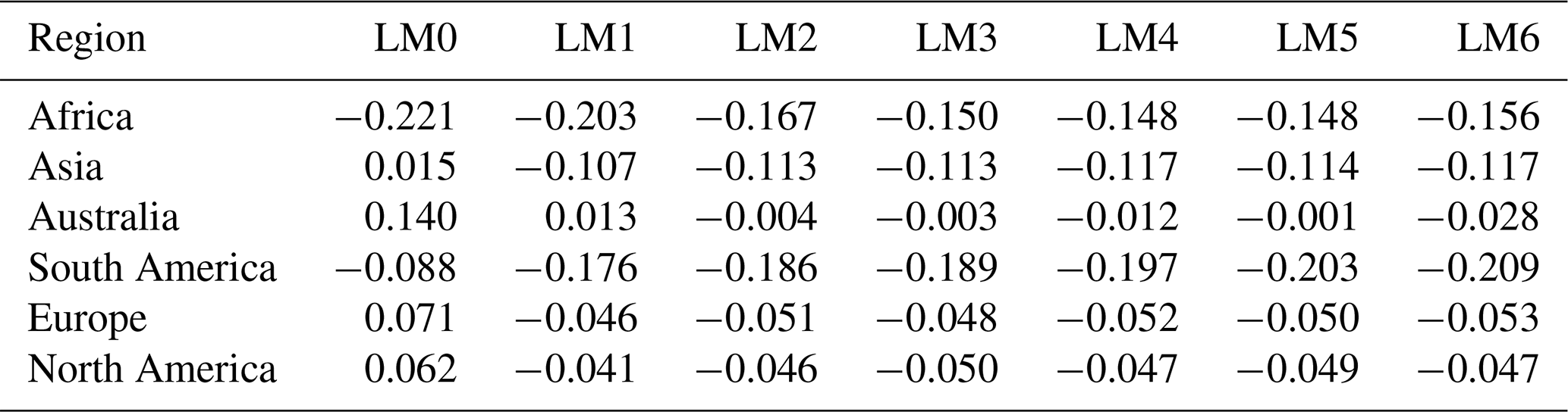
In the first lead month (approx. 30–60 d after initialization) the forecast already exhibits substantial bias for both variables on a global scale when using uncorrected forecasts (Fig. 1). As illustrated in the left panel of Fig. 1, the most pronounced loss of skill for precipitation during the reference period occurs in arid and semi-arid regions. In terms of absolute precipitation amounts, however, the largest biases are found in tropical regions, with missing precipitation over the Amazon basin and an overestimation in the Congo basin. For temperature, most land areas exhibit a cold bias, which is particularly pronounced over the Sahara and in mountainous regions. For both variables, distinct wave-like patterns are visible, especially along major mountain ranges. These patterns may originate from deficiencies in the representation of orographic gravity wave drag or, more systematically, from spectral parameterizations in the original model output that are transferred to the Gaussian grid during post-processing. The presence of these biases results in negative global skill scores for the uncorrected forecasts (Table A1). With increasing lead time, systematic drift becomes even more pronounced (Table A1), further degrading forecast performance relative to the climatology. This highlights the urgent need for bias correction to adjust forecasted values toward more realistic levels.

To quantify these skill levels more systematically across space and lead time, we next examine the CRPSS values aggregated by lead month and region. Figure 2 provides a detailed global assessment of the BCSD forecasts using the CRPSS. Across nearly all land regions, BCSD outperforms the climatology by a large margin, with particularly strong gains observed for temperature. For both meteorological variables and the drought indicator, Lead Month 0 exhibits high skill, with values exceeding 0.15 globally for precipitation and SPEI-1, and 0.25 for temperature in many regions. Bootstrap resampling with 1000 iterations confirms that these positive skill values are statistically robust over most land regions (Fig. A5). Starting from Lead Month 1, a noticeable decline in skill is observed. In Lead Months 1–3, CRPSS values decrease globally and fewer regions retain statistically robust positive skill according to the bootstrap analysis. Nevertheless, 69.7 % of all grid cells still show skillful precipitation forecasts relative to the climatology, and 97.4 % for temperature. For SPEI-1, 88.8 % of grid cells retain positive skill. While the bootstrap analysis indicates increased uncertainty at longer lead times, positive skill remains evident across large parts of the globe. The CRPSS difference between BCSD-corrected and uncorrected forecasts (not shown) remains relatively stable across the subsequent lead months, indicating that all forecast horizons benefit similarly from the BCSD correction. The best performing regions are concentrated around the equator, while areas with lower skill include Central Russia for both variables, and the Sahara for precipitation. In Lead Months 4–6, the spatial pattern remains similar. Robust positive regions are concentrated around the equator. As expected, skill decreases with increasing lead time, though many regions still retain positive skill values. Notably, the spatial extent of robust positive skill is substantially larger for SPEI-1 than for precipitation alone. This suggests that drought indicators integrating both precipitation and temperature information can provide a more stable and predictable representation of water-balance anomalies than precipitation by itself.

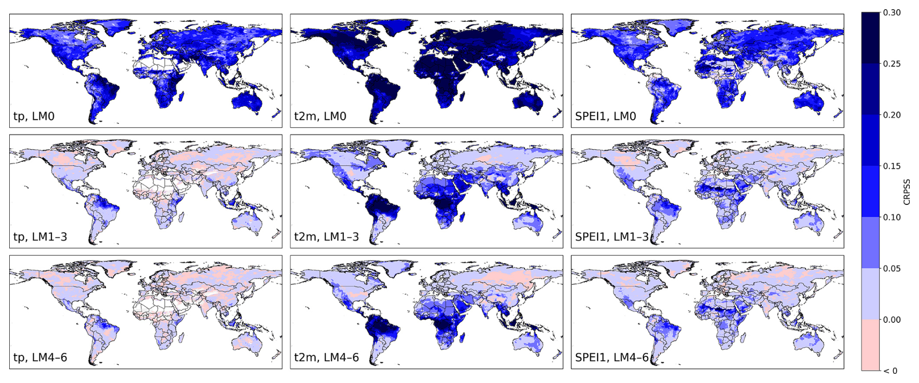
Figure 2 SEAS5-BCSD, Continuous Ranked Probability Skill Score relative to climatology for different lead months (LMs), shown for precipitation (left) and temperature (middle) and SPEI-1 (right). Lead Month 0 (top), Lead Months 1–3 (middle), and Lead Months 4–6 (bottom) are displayed. Blue colors indicate higher skill than climatology, with darker shades representing better performance. Dry grid cells are excluded.

Since skill in average conditions does not always translate to skill in extremes, we complement the CRPSS analysis with a categorical assessment based on probabilistic thresholds. Accordingly, Fig. 3 provides a more detailed evaluation of Brier Skill Score (BSS) performance across several drought and wetness thresholds. The figure includes the widely used tercile thresholds (top row), quintile thresholds (third row), and the 10th and 90th percentiles (second row), the latter serving as proxies for more extreme events. For the categories in-between, the middle tercile and quintile categories is shown in the bottom row. These “normal conditions” forecasts exhibit far less skill than the dry/wet categories with only a relatively weak BSS values evident even in Lead Month 0. In contrast, forecasts for dry and wet categories demonstrate significantly higher skill. Evaluating the percentage of land area with positive BSS values, the tercile approach achieves the highest coverage with 99.1 % (dry) and 99.4 % (wet), followed closely by the quintile approach with 96.8 % and 98.5 %, respectively. In terms of the magnitude of skill, the tercile-based forecasts also show higher mean BSS values overall. The main regional difference between the tercile and quintile approaches are concentrated in North-East Asia, where quintile skill is somewhat reduced. For the more extreme categories, skill is not symmetrically distributed between the wet and dry ends of the spectrum: while wet extremes are predicted with similar skill to the corresponding tercile and quintile categories, forecasts for dry extremes show reduced skill in several regions, particularly compared to their wet counterparts. For temperature (Fig. A1), overall skill is higher, both in terms of the fraction of positively skilled grid cells and the magnitude of the BSS values. Only a few regions in the Himalayas display reduced skill in the tercile categories, along with negative skill in the quintile and extreme categories. In contrast to precipitation, the forecast performance for hot and cold anomalies is nearly symmetrical. However, as with precipitation, categories representing “near-normal” conditions show substantially reduced skill.

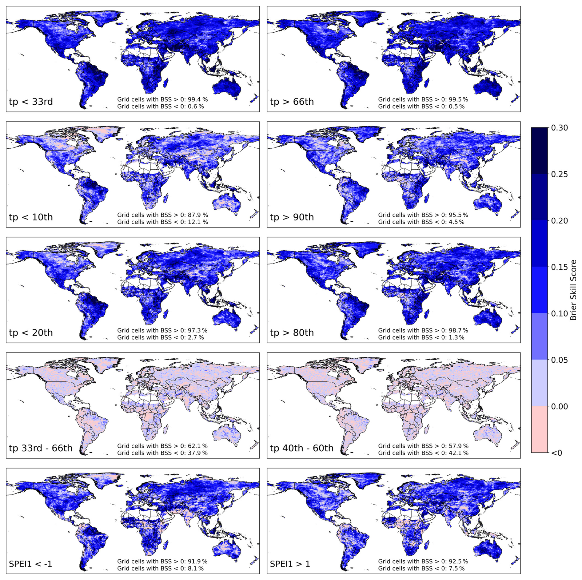
Figure 3 SEAS5-BCSD, Brier Skill Score (BSS) relative to climatology for precipitation, as well as SPEI-1, at Lead Month 0. Different percentile thresholds are shown, indicated in the lower-left corner of each panel. Blue colors indicate higher skill than climatology, with darker shades representing better performance. Dry grid cells are excluded.

Additionally, Fig. 3 includes the BSS for SPEI-1 conditions. In this case, the commonly used thresholds of $\text{SPEI}<-\mathrm{1}$ and SPEI>1, representing drought and wet conditions, respectively, are applied instead of percentile-based categories. Most regions exhibit positive skill for both drought and wet conditions. Regions with limited or no skill include parts of Sub-Saharan Africa, northern South America, and India. Since SPEI thresholds of −1 and 1 are not directly equivalent to the percentile thresholds shown for precipitation and temperature, a direct comparison of skill magnitudes is not possible. Nevertheless, comparison of the spatial patterns suggests that the reduced skill over Sub-Saharan Africa is more closely associated with the temperature component, whereas the deficits in northern South America and India appear to be linked primarily to precipitation or to a combination of both variables. Overall, the magnitude of the SPEI-1 skill is more comparable to that of precipitation than temperature, indicating a stronger influence of precipitation variability on SPEI-1. Despite regional differences, drought and wet conditions generally show higher skill than climatology across most regions.

Since the forecasts in Lead Month 0 for abnormal dry conditions (below the 33rd percentile) perform best, a closer inspection of subsequent lead times is warranted. As expected, the spatial extent of regions with positive skill decreases with increasing lead time (Fig. 4). In most parts of the world, this decline appears gradual. A notable exception is Central Europe, where skill drops substantially in Lead Month 1 before improving again in later months. Regions exhibiting strong skill in LM0 (cf. Fig. 3), such as northern Brazil, Mexico, Indonesia, and southern Africa, generally maintain positive skill through LM6. In contrast, other areas like Australia and India show a marked reduction in predictive skill at longer lead times. High-latitude regions, including boreal Canada and Siberia, exhibit only weak signals throughout. When turning to above average temperature forecasts (see Fig. A2), a stronger and more spatially consistent skill is evident, even at longer lead times such as LM6. The equatorial region again shows particularly strong performance, other than that no obvious spatial pattern arise. Overall, Brier Skill Score values for temperature substantially exceed those of precipitation, especially for lead times further in the future, underlining the comparatively higher predictability of temperature on seasonal scales.

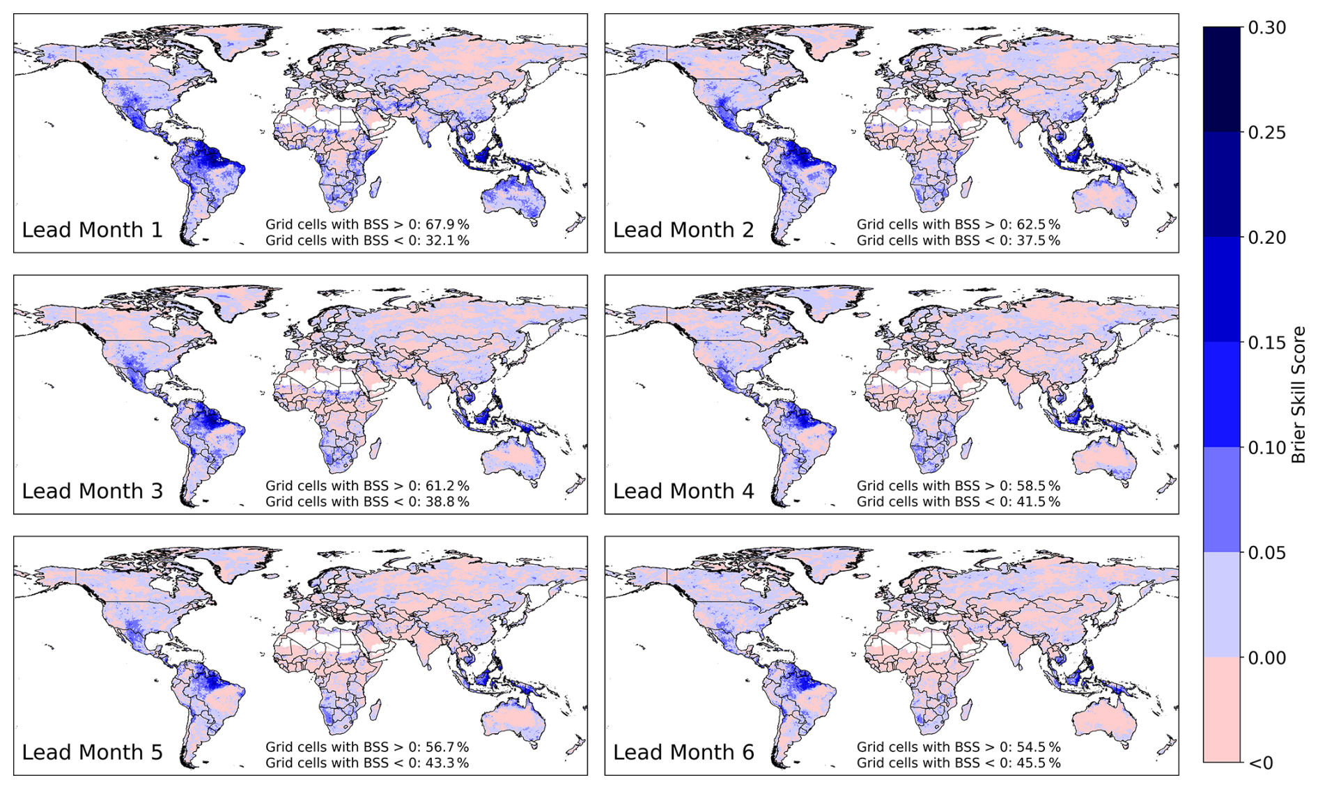
Figure 4 SEAS5-BCSD, Brier Skill Score (BSS) relative to climatology for precipitation, focusing on dry conditions below the 33rd percentile for Lead Months 1–6. Blue colors indicate higher skill than climatology, with darker shades representing better performance. Dry grid cells are excluded.

3.2 Statistical consistency and predictive characteristics

To complement the regional analysis, a statistical evaluation of the dataset is provided. An essential requirement for the BCSD method is that it does not shift the distribution of the values into unrealistic territory. In particular, during the reference period, the statistical characteristics of the bias-corrected SEAS5 values should align closely with that of ERA5 due to the quantile mapping approach. Figure 5 illustrates this by showing the distribution of BCSD-corrected SEAS5 monthly precipitation values from 1981 to 2016. The bin thresholds are defined by ERA5 percentiles (5th, 10th, 15th, …, 95th), resulting in bins that each contain 5 % of the ERA5 data. The SEAS5 data would also be uniformly distributed across these bins, although perfect agreement is not expected because the bias correction is applied at the daily scale, while the analysis is based on monthly means. The histogram confirms a strong agreement between ERA5 and SEAS5, particularly the precipitation values above 0.5 mm d⁻¹ are all in perfect proportion to the expected 5 %. In the very dry categories, a slight underrepresentation of the driest two bins is noted, with an overrepresentation in the adjacent (still dry) bins. This discrepancy becomes more pronounced in later lead months but remains minor in Lead Month 0. Additionally, a marginal underrepresentation is noted in the wettest bins, though this effect is negligible.

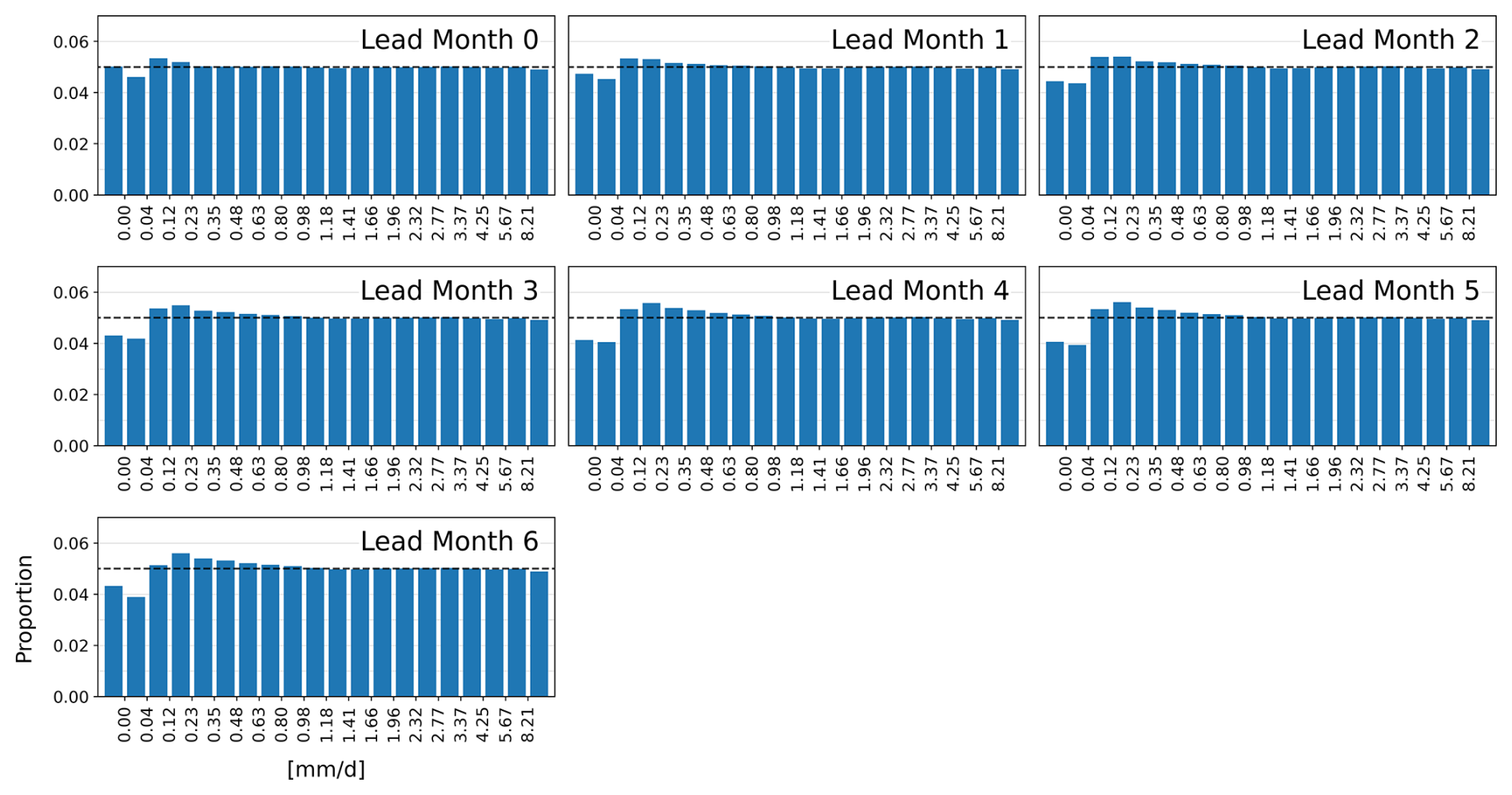
Figure 5 Histogram of BCSD-corrected SEAS5 monthly precipitation values for the period 1981–2016. Bin thresholds are defined by ERA5 percentiles (5th to 95th), such that each bin contains 5 % of the ERA5 data. A uniform distribution of SEAS5 values across bins would indicate perfect agreement with the ERA5 reference distribution.

While the histogram confirms the consistency of the corrected forecast distribution, it does not reflect the forecasting system's ability to correctly anticipate event occurrence. To address this, we turn to the Receiver Operating Characteristics (ROC) analysis. Figure 6 shows values left of the 1:1 diagonal for all variables, lead months and percentile thresholds, the area under the ROC curve (AUC) exceeds 0.5, indicating positive skill relative to a climatological forecast. In Lead Month 0, skill levels are high across both temperature and precipitation. In Lead Month 1, forecast performance decreases, particularly for precipitation, but remains skillful. These findings are consistent with earlier assessments in Figs. 4 and 2. Temperature forecasts maintain robust discriminatory power, with ROC curves for Lead Month 1 still comparable to the precipitation performance in Lead Month 0. Among percentile categories, only marginal differences are observed; with the only exception being a slightly better performance of the dry categories in Lead Month 0 of precipitation, suggesting improved detectability of dry conditions at shorter lead times when the classification threshold is low. To assess the robustness of these results, bootstrap confidence intervals were estimated from 1000 resampling iterations and are shown as shaded areas in Fig. 6. For precipitation, the confidence bands are extremely narrow and barely visible, indicating a high degree of consistency across years. For temperature, the spread is somewhat larger but remains limited, with all curves clearly indicating positive skill. The narrow confidence intervals may partly reflect the spatial aggregation applied in this analysis, as regional differences can compensate each other in the global mean.

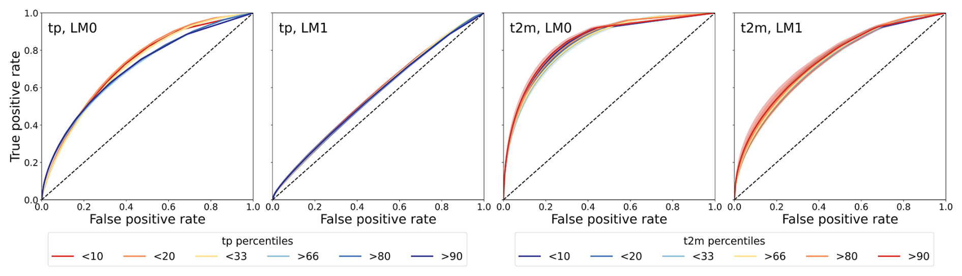
Figure 6 SEAS5-BCSD, Receiver Operating Characteristic (ROC) curves for precipitation (left) and mean 2 m temperature (right) for Lead Months 0 and 1. Percentile thresholds are used to distinguish between abnormal and strong dry/wet conditions. Shading indicates the 1st–99th percentile range obtained from 1000 bootstrap resamples. The dashed line indicates random chance.

Building on this evaluation, we investigate whether internal ensemble agreement correlates with forecast skill, providing further insights into forecast confidence. Figure 7 explores the role of ensemble agreement, a component already implicitly considered in CRPSS and BSS, in greater detail. The graph illustrates how forecast skill varies across different percentile thresholds as a function of ensemble agreement, i.e. the proportion of ensemble members falling into a given category. This proportion can be interpreted as a measure of internal certainty within the SEAS5 forecast system. For the 20th and 33rd percentiles (representing dry conditions), forecast skill improves constantly with increasing ensemble agreement above a percentage of 33 % on the x axis, corresponding to the threshold to a possible majority in tercile analysis. This suggests that the greater the confidence of the ensemble in predicting dry conditions, the better the forecast performance. For more extreme dryness (10th percentile), a similar trend is observed up to an ensemble share of 20 %, although at generally lower skill levels. Beyond this point, the curve plateaus and then falls off, though the number of such cases becomes sparse, limiting interpretability. In contrast, for wet conditions, the relationship between the wet, strong wet and extreme wet categories is near identical. Nevertheless, across all percentiles and categories, forecast skill generally remains in the positive range for Lead Month 0, with the exception of extreme droughts. In summary, for most threshold categories, a higher degree of ensemble agreement correlates with better forecast performance, highlighting the added value of ensemble certainty in probabilistic seasonal predictions.

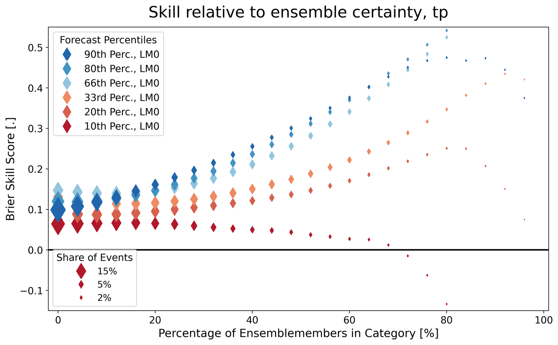
Figure 7 SEAS5-BCSD, Brier Skill Score (BSS) relative to climatology as a function of the number of ensemble members within a category, shown for precipitation at Lead Month 0. Three drought/wet thresholds are depicted. The size of the rectangles denotes the share of events.

We further assess how forecasts persist and evolve as new initialization dates approach the target month, a key aspect for users requiring early, reliable warnings. While Fig. 7 focused on selected percentile thresholds, it is equally important to assess the full distribution of ensemble members. Figure 8 illustrates how SEAS5 forecasts are distributed across tercile categories, conditional on the ERA5 classification. For example, the top-left panel includes only those grid cells where ERA5 indicates wetter-than-normal conditions. The bars then show the share of the forecasted classes for these grid cells with lead times from seven (leftmost bar per plot) to one month ahead. A purely climatological forecast would distribute 33.3 % of cases into each tercile. Thus, if the bars with the darker hue exceed 33.3 %, SEAS5 outperforms climatology. A clear trend emerges: the closer the forecast issue date is to the target month, the more accurate the tercile classification. From Lead Month 6 to Lead Month 1, this improvement is gradual, followed by a significant jump in performance at Lead Month 0. With regard to precipitation, dry conditions are most reliably predicted. When dry conditions occur, SEAS5 forecast already indicated them three months in advance with a 19 % higher probability than climatology. Conversely, “normal” conditions are more difficult to capture and are not predicted more accurately than climatology at any lead time. As observed in previous figures, temperature forecasts show higher skill than precipitation, except in the “normal” tercile, which remains below climatological skill. However, when ERA5 indicates unusually warm conditions, the BCSD-corrected forecasts captured this correctly in half of all cases in Lead Month 2, 50 % better than the one-in-three expectation from climatology. Figure 8 can also be interpreted from the opposite perspective by examining the rate of incorrect, reversed forecasts, i.e. instances where the predicted tercile was opposite to the observed category. This provides insight into the potential risks for users relying on categorical forecasts. For example, when ERA5 indicated dry conditions, 29 % of forecasts predicted wet conditions two months prior, dropping to just 16 % at Lead Month 0. Similarly, for hot months, only a fourth of the grid cells predicted cold conditions half a year ahead, and this number decreased to 10 % one month in advance.

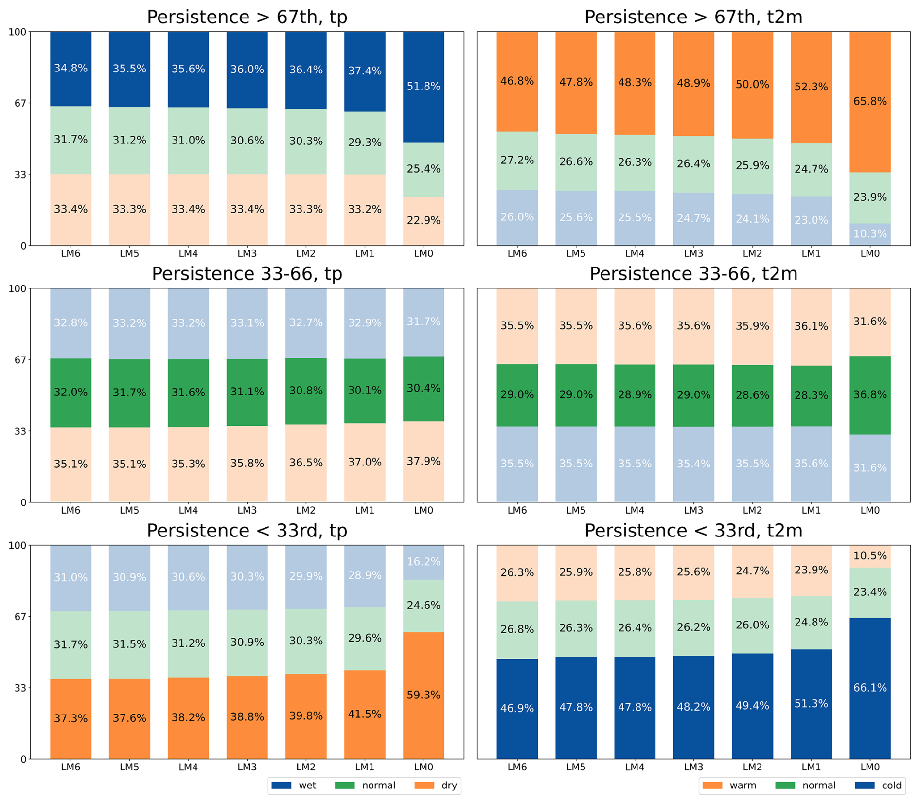
Figure 8 SEAS5-BCSD, Tercile persistence for precipitation (left) and temperature (right). For each ERA5-classified tercile, the corresponding SEAS5 tercile classifications are tracked across the seven lead months. Values represent percentage distributions aggregated over all grid cells and the reference period. Darker shading indicates the correct (persistent) category.

The longer a condition is consistently forecasted across subsequent issue months, the higher the forecast skill becomes. For drought conditions, the tercile hit rate for Lead Month 0 reaches 49.6 %, corresponding to 17.7×10⁶ correctly predicted grid cells out of 35.8×10⁶ grid cells that showed drought condition in LM0. If the same month was already predicted as dry one issue month earlier, this rate increases slightly to 50.2 % (8.2×10⁶ of 16.3×10⁶ grid cells). Including predictions from Lead Months 2–6 from preceding issue months leads to a steady improvement in skill, rising to 50.8 % (4.7 of 9.3×10⁶), 51.4 % (3.1 of 6.0×10⁶), 52.0 % (2.2 of 4.2×10⁶), 52.6 % (1.6 of 3.1×10⁶), and 53.3 % (1.2 of 2.3×10⁶), respectively. This effect is even more pronounced for mean temperature, with more cases of consistent forecasting as well. Starting from a hit rate of 61.3 % (22.2 of 36.1×10⁶) for Lead Month 0, the rate increases markedly with each earlier forecast: 64.9 % (13.1 of 20.2×10⁶) for Lead Month 1, 66.4 % (9.5 of 14.2×10⁶), 67.7 % (7.5 of 11.1×10⁶), 68.9 % (6.2 of 9.0×10⁶), 70.0 % (5.3 of 7.6×10⁶), and finally 70.8 % (4.6 of 6.5×10⁶) when considering forecasts from Lead Month 6.

3.3 Forecast skill in further context

The preceding analyses and figures showed that the skill of precipitation forecasts has clear limitations on a global scale. The global CRPSS (cf. Fig. 2) indicates relatively high performance in equatorial regions and poor performance in subtropical, arid zones. To investigate this relationship more systematically, each grid cell was assigned to a specific climate zone according to the Köppen–Geiger Climate Classification (Beck et al., 2018). Figure 9 illustrates the typical pattern: high skill in Lead Month 0 followed by a stagnation or gradual decline in subsequent lead months. Among the different climate zones, the tropical regions clearly stand out with the highest forecast skill for precipitation. Most months in these regions maintain positive skill even at Lead Month 6. In contrast, the neighboring arid zones are already outperformed by climatology from Lead Month 2 onward. At this lead time, forecasts for temperate and polar regions still retain a slight advantage over climatology, though their skill converges toward zero at longer lead times. Cold regions perform similarly to arid ones in terms of CRPSS, albeit with a narrower spread. To quantify the benefit of the BCSD correction across climate zones, we also computed the CRPSS relative to the raw SEAS5 forecasts (not shown). The tropics again show the strongest improvement, with a median CRPSS gain of 0.28, followed by temperate zones (0.15), arid (0.11, with substantial spread), polar (0.07), and cold regions (0.06). Differences between lead months are minor, suggesting that tropical precipitation forecasts benefit most consistently and substantially from the BCSD approach.

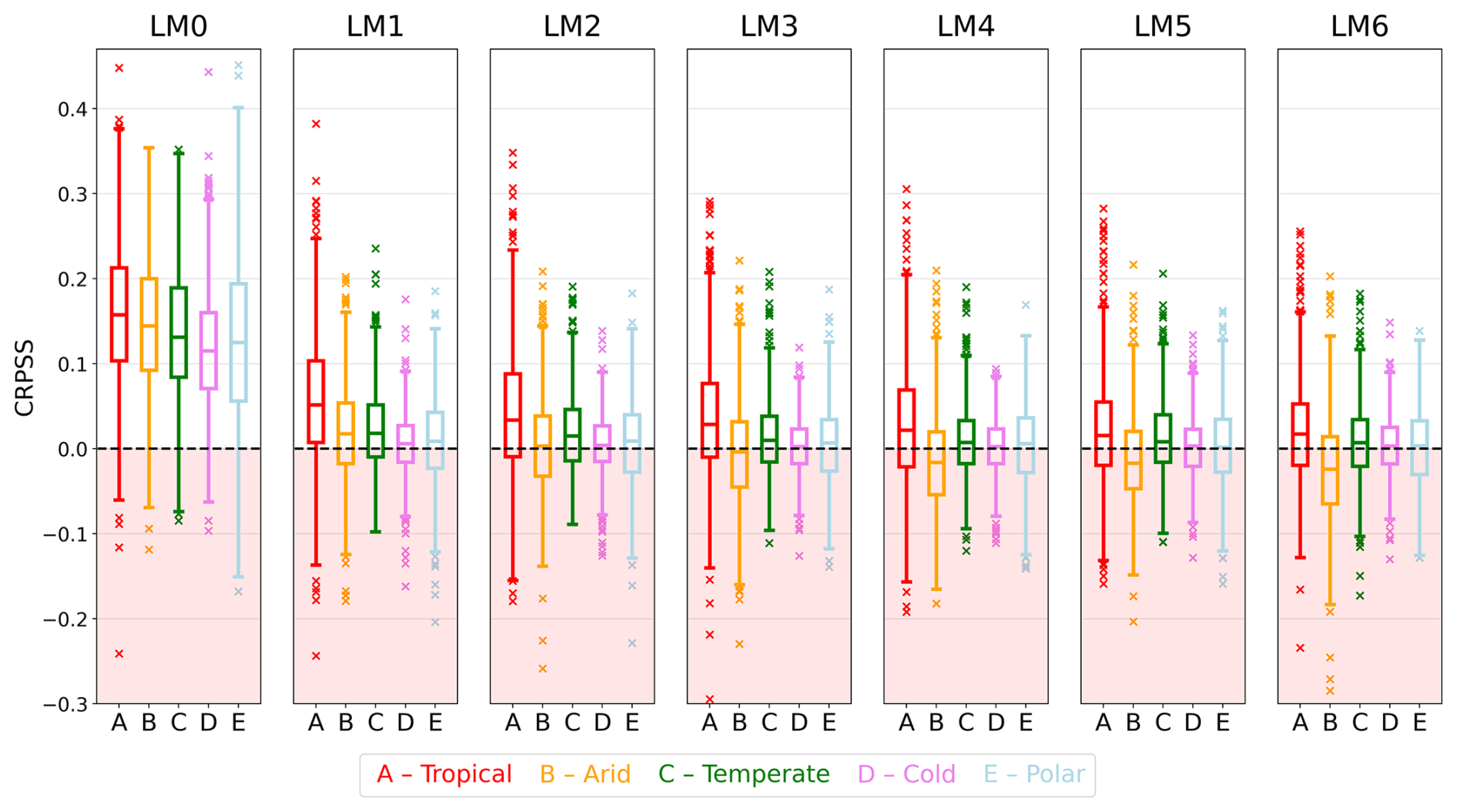
Figure 9 SEAS5-BCSD, Spatially aggregated Continuous Ranked Probability Skill Score (CRPSS) relative to climatology for precipitation, shown for Lead Months 0–6 over the period 1981–2016. Results are grouped by major climate classes according to the Köppen–Geiger classification.

Figure 2 reveals a performance bias toward hot or cold conditions in Lead Months 1–6, but in Lead Month 0, this is not apparent. One potential factor influencing temperature forecast skill is elevation. Raw SEAS5 forecasts have strong biases in mountain areas (Fig. 1, right panel), which the BCSD should reduce. By isolating elevation effects, more nuanced insights may emerge for Lead Month 0. Seasonal forecasting in mountainous regions is particularly challenging (Uttarwar et al., 2025). To assess the potential influence of elevation on temperature forecast skill, Fig. 10 shows the CRPSS for different elevation-related metrics for Lead Month 0. Elevation data are derived from the 30 m-resolution TanDEM-X Global DEM (Gonzalez et al., 2020), aggregated to match the 0.25° ERA5 grid. On the left, the mean elevation per grid cell is shown. A clear trend emerges: for Lead Month 0, CRPSS values are highest in lower-lying regions and tend to decrease gradually with increasing elevation. To investigate whether this trend is more related to absolute peak elevation or general plateau height, CRPSS is also shown for the maximum and minimum elevations. Maximum elevation displays a pronounced stratification, suggesting that the presence of low-lying terrain is more conducive to higher forecast skill than regions with high peaks. In high plateaus or mountain ranges, where all grid cells lie above 3000 m, the temperature forecast skill is somewhat reduced, as seen in the third panel from the left. Additionally, terrain complexity, calculated as the mean absolute difference from the mean elevation, also correlates with skill, though less strongly than mean elevation.

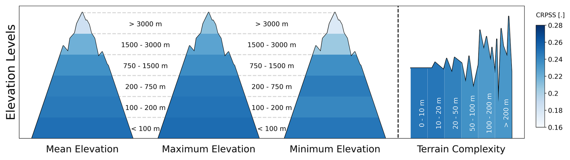
Figure 10 SEAS5-BCSD, CRPSS of temperature for Lead Month 0, stratified by elevation metrics. Mean elevation refers to the average value of the high-resolution DEM within each grid cell, maximum elevation denotes the highest point, and minimum elevation the lowest. Terrain complexity is defined as the mean absolute deviation of all high-resolution DEM values from the grid cell mean.

Given the apparent relationship between forecast skill and annual precipitation totals (see Fig. A3), a more detailed investigation of this dependency is warranted. A clear positive relationship can be observed: the greater the rainfall amount, the higher the forecast skill. As the CRPSS is a normalized score comparing forecasts to climatology, this trend cannot be attributed to larger absolute errors at high precipitation values, as is the case for metrics like CRPS or mean absolute error. This relationship aids in interpreting the spatial skill patterns shown in Fig. 4. Regions with higher annual precipitation generally correspond to areas of improved forecast skill. Since Fig. 4 displays skill for drought forecasts, already arid regions inherently exhibit lower Brier Skill Scores, as drought conditions are climatologically common and thus harder to distinguish from the baseline. This relationship is particularly evident in Central Australia, where low precipitation levels coincide with low skill values in the BCSD-corrected forecasts. The highest forecast performance is found in regions receiving more than 2000 mm yr⁻¹, beyond which the performance curve flattens. At the other end of the spectrum, regions with low precipitation amounts show a clear decline in skill (see Fig. A3). For Lead Month 6, the CRPSS values begin to fall consistently below zero at around 330 mm yr⁻¹ (not shown). Forecasts closer to the target month maintain positive skill down to lower precipitation thresholds, with the transition points at approximately 10, 90, 195, 205, 305, and 235 mm yr⁻¹ for Lead Months 0 through 5, respectively. Below these thresholds, forecast performance declines rapidly. An interesting pattern emerges for Lead Month 0: in arid (but not hyper-arid) regions with less than 250 mm yr⁻¹, forecast skill slightly increases as precipitation decreases, peaking around 30 mm yr⁻¹. This may reflect the relatively good performance of the system in predicting drought conditions in these dry environments.

In the vicinity of 300 mm yr⁻¹, where forecast skill becomes consistently positive, albeit at a low level, many semi-arid regions of the Earth are located, typically characterized by a pronounced rainy–dry season cycle. These two seasons often differ markedly in their observed and forecasted rainfall amounts. To assess their impact separately, Fig. 11 presents a seasonal analysis based on the Brier Skill Score (BSS). Only regions with a strong seasonality were included, defined as those where the two driest months contribute less than 20 % of the rainfall of the two wettest months. Very arid areas with annual totals below 250 mm yr⁻¹ were excluded. The upper graph is subdivided into three horizontal sections corresponding to the forecast skill for mild (top row), moderate (middle), and severe droughts (bottom). For Lead Month 0, all categories show positive skill in both seasons. While the rainy season maintains positive skill throughout the entire lead time range, forecast performance during the dry season quickly deteriorates, with BSS values turning negative after one month. In contrast, seasonal variation in the mid-latitudes is primarily temperature-driven. Accordingly, Fig. 11 also shows BSS values for summer and winter in regions where the three warmest months are at least 10 °C warmer than the three coldest. In these areas, seasonal differences in forecast skill are less pronounced. For hot and moderate warm seasons (again, relative and not absolute), winter exhibits slightly better performance. However, in the case of mild seasons (bottom row), the differences between winter and summer largely vanish.

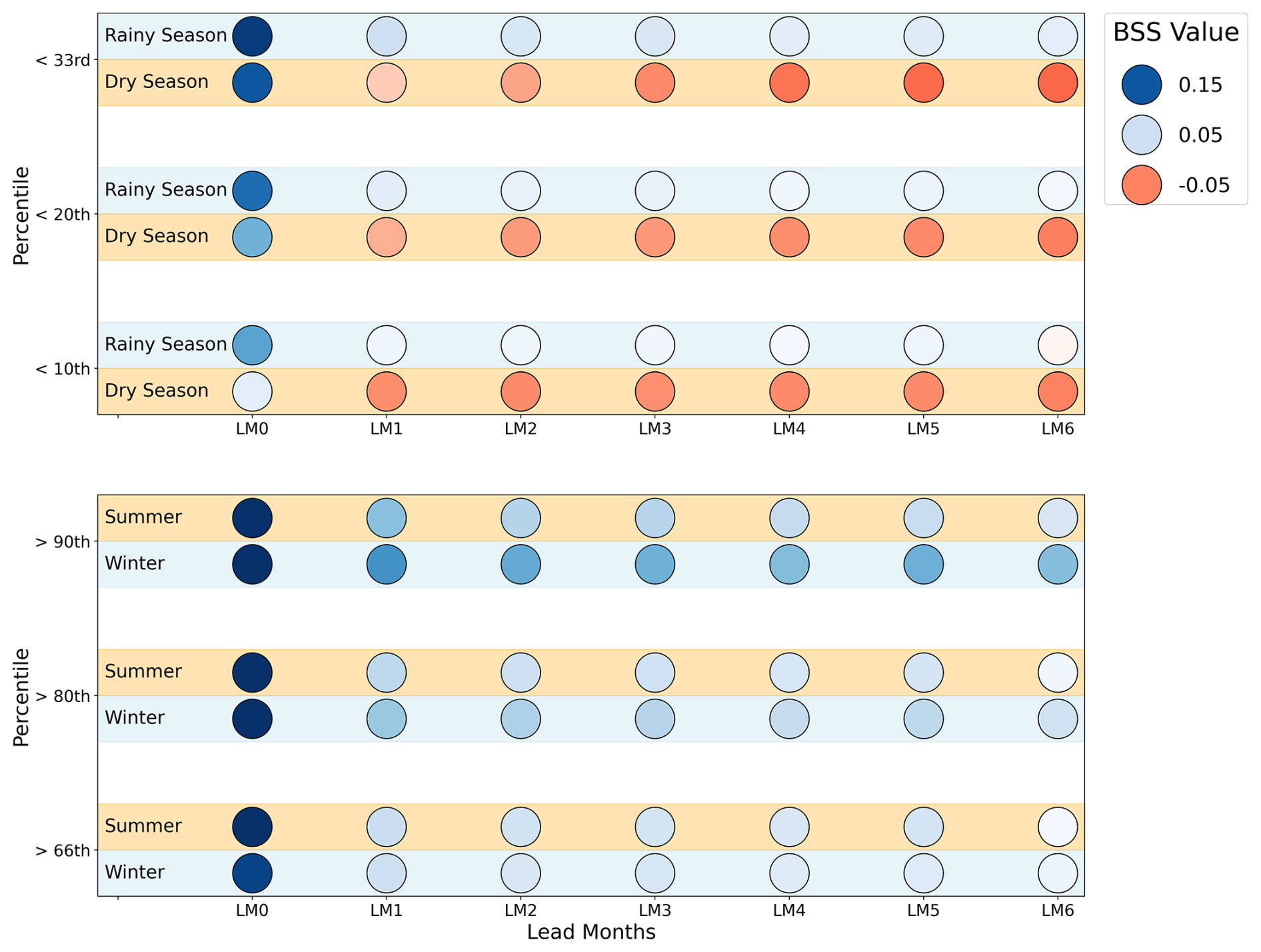
Figure 11 Brier Skill Score (BSS) for different seasons. Precipitation is separated into rainy and dry seasons (top panel), temperature into summer and winter seasons (bottom panel). The color intensity is proportional to the BSS value.

4 Discussion

Our findings stress the variability in seasonal forecast performance across different climate regimes and conditions. Particularly noteworthy is the limited forecast skill in arid regions, which warrants closer examination in the following discussion.

4.1 Underperformance in arid regions/Climate-dependend performance

The analysis revealed that BCSD forecasts tend to be outperformed by climatology in arid regions. This is supported by regional studies, such as Zamora et al. (2021), who found a weak Brier Skill Score for extremely dry predictions in the US using a different seasonal forecasting product. Thrasher et al. (2012) also discussed the limitations of BCSD performance over extreme climates. One likely reason for this skill deficit is the low signal-to-noise ratio in dry regions: the absolute differences between dry and very dry conditions are small, making them more difficult to predict accurately (Hao et al., 2018). Even minor biases or shifts in forecast distribution can therefore result in a loss of skill relative to climatology. To assess whether the observed skill reduction originates from the bias correction method itself or from limitations in the SEAS5 model (which was developed after the study by Thrasher et al., 2012) Fig. 5 provides further insight. It shows that the lowest precipitation values are slightly underrepresented, while marginally wetter (but still dry) categories are correspondingly overrepresented. Before the bias correction, SEAS5 forecasts contain more days without precipitation over land than ERA5, typical for climate prediction systems due to the drizzle effect (Boé et al., 2007). The BCSD process appears to reverse this pattern. Wetter categories are represented very well in contrast. This discrepancy may point to limitations in how dry-day probabilities (DDP) are handled by the system. In the context of climate projections, Rajczak et al. (2016) demonstrated that Quantile Mapping can significantly improve the representation of dry spell lengths in comparison to overly wet raw projections, thereby also enhancing the accuracy of DDP estimates. This is supported by Themeßl et al. (2012), although for RCMs not for seasonal forecasting systems. On the other hand, Maraun (2013) reported that Quantile Mapping struggles with correctly adjusting drizzle precipitation, highlighting limitations in handling low-intensity events. As described in Sect. 2.2, if the DDP of SEAS5 is larger than of the reference, random sampling is applied to draw values from the respective cumulative distribution function (CDF). If the fixed number of quantile bins (200) is insufficiently granular, this can lead to mismatches. Since SEAS5 generally exhibits slightly more dry days, this issue is more frequent than in the reverse case, where values are forced to zero in the correction. A further contributing factor could be the temporal smoothing introduced by the 31 d moving window used in the correction process. In very dry months, this may result in contamination by wetter days from neighboring seasons, shifting values into higher bins (e.g. from the lowest to the third-lowest category) based on very small differences (border at 1.2 mm month⁻¹). Additionally, monthly averaging may amplify the influence of individual forecasted precipitation events. This could result in SEAS5 displaying non-zero values even in months with extremely low actual rainfall, potentially skewing distributions further.

4.2 Limitations

Pixel-wise Empirical Quantile Mapping (EQM) was selected as the bias-correction approach because it corrects the full local distribution of the forecast variables, including distribution tails, dry-day frequencies, and percentile-dependent biases. This is particularly important for the representation of extremes such as droughts, as precipitation distributions are highly non-Gaussian and strongly region-dependent (Lorenz et al., 2021). In addition, the pixel-wise formulation allows heterogeneous regions, for example coastlines or mountainous terrain, to be treated independently, resulting in locally consistent corrected fields (Eden et al., 2012). Since the correction is applied at daily scale prior to temporal aggregation, sub-monthly variability and accumulated drought characteristics are preserved more realistically (Themeßl et al., 2012). However, the approach also has limitations. As with all observation-based bias-correction methods, EQM depends on the quality of the reference dataset (see below); therefore, systematic biases present in ERA5 may propagate into the corrected forecasts (Maraun, 2013). Furthermore, the method does not explicitly correct spatial dependence structures or displacement errors, which can in some cases reduce spatial coherence in the corrected precipitation fields. Like many statistical bias-correction approaches, EQM additionally assumes temporal stationarity between model biases in the calibration and application periods.

Alternative calibration approaches, such as mean-variance calibration (e.g. Doblas-Reyes et al., 2013a), are primarily designed to improve large-scale forecast skill and ensemble reliability while preserving the characteristics of the original forecast system. Such approaches are particularly advantageous for studies focusing on teleconnections, climate variability, or predictability. However, they generally do not correct distributional biases beyond the first moments and may therefore inadequately represent highly skewed variables such as precipitation and their associated extremes. By contrast, distribution-based methods such as EQM explicitly correct the full local distribution and have therefore become widely used in the development of impact-oriented meteorological datasets and bias-corrected seasonal forecast products. Since the primary objective of SEAS5-BCSD is not the optimization of large-scale ensemble-mean skill, but the generation of realistic meteorological fields for drought analysis and downstream applications at high spatial resolution, the accurate representation of local distributions, dry-day frequencies, and extreme events was considered more important than preserving the raw ensemble characteristics. For these intended applications, EQM therefore represents a suitable compromise despite its known limitations.

Empirical Quantile Mapping assumes that the relationship between model and reference distributions remains sufficiently stable between calibration and application periods. Given the strong warming trend during 1981–2016, potential non-stationarity represents an important source of uncertainty. To assess this, the temporal evolution of the large-scale SEAS5 temperature bias was examined (Fig. A4). Although ERA5 exhibits a pronounced warming trend, the relative cold bias of SEAS5 remains comparatively stable throughout the hindcast period, and no clear evidence of a large-scale temporal drift in the aggregated bias was found. Precipitation biases show stronger interannual variability and spatial heterogeneity, but no pronounced large-scale temporal trend was identified in the globally aggregated mean bias. Nevertheless, residual non-stationarity cannot be excluded, particularly under continued climate change. It should also be noted that much of the hindcast period overlaps with the 1981–2010 climatological reference period recommended by the WMO for many operational applications. Furthermore, unlike bias correction of long-term climate projections, seasonal forecasts are initialized from the contemporary climate state and therefore already incorporate much of the underlying large-scale warming signal. Consequently, the stationarity assumption underlying empirical quantile mapping is expected to be less restrictive for seasonal forecasts than for century-scale climate projections, although some uncertainty associated with evolving model biases remains.

Despite its widespread use as a reference, ERA5 is not without limitations, particularly in data-sparse regions and for variables like precipitation, where reanalysis uncertainties can propagate into both forecast evaluation and bias correction. For Ethiopia, Ahmed et al. (2024) found that CHIRPS generally outperformed ERA5, especially in the Ethiopian Highlands, where both datasets overestimated rainfall and underestimated the observed high rainfall variabilities. However, ERA5 is able to reasonably capture spatial patterns and rainfall distribution. On a global scale, ERA5 also exhibits a slight wet bias, but performs well in extratropical regions, particularly for precipitation (Lavers et al., 2022). Comparisons with satellite-based products such as IMERG over China suggest that ERA5 performs less well in tropical regions, but tends to outperform satellite datasets in continental and cold temperate areas (Xu et al., 2022). Despite these known limitations, ERA5 was chosen as the reference for this study due to its overall adequate performance, full global coverage and near real-time availability with only a short latency of five days. Additionally, ERA5 offers consistent data across multiple variables, facilitating a seamless transition between precipitation and temperature analyses and bias correction approaches. We acknowledge that trend calculation in ERA5 is not recommended. However, since the BCSD method also relies on this reference dataset, the comparison remains valid. The same trend effects should be reproduced when using different datasets as input for the CDFs. It should be noted that ERA5 is not an independent observational reference but a reanalysis product that is also used as the target for bias correction. Consequently, the evaluation primarily assesses consistency with the reference dataset rather than absolute forecast skill against independent observations.

4.3 Computational efficiency

Timely availability of bias-corrected forecasts is crucial, particularly since forecast skill is shown to be highest during the first lead month. As SEAS5 forecasts are released on the 5th of each month at 12:00 UTC, our goal was to produce BCSD-corrected outputs for six variables on the same day. To meet this target, we needed to make substantial efforts to reduce computational demand. The primary improvement in computational efficiency stems from storing pre-computed cumulative distribution functions (CDFs), rather than generating them on-the-fly, as done in previous studies (e.g. Lorenz et al., 2021). To reduce processing time during the CDF preparation stage, we approximated the empirical CDFs using a reduced number of quantile points: 200 instead of the full set of available values (1116 for ERA5 and 27 900 for SEAS5). This linear interpolation approach is widely used in the literature (e.g. Themeßl et al., 2012; Boé et al., 2007) and reflects a compromise between computational efficiency and statistical accuracy. Although higher-resolution CDFs (e.g. 500 or full data) may enhance correction performance (Gudmundsson et al., 2012), test runs demonstrated only marginal differences in forecast skill between 200, 500, and the full dataset. In contrast, using only 100 points led to noticeable degradation in performance. Therefore, 200 quantile points were selected as a balanced solution. This reduction also resulted in significantly lower storage requirements, with the pre-computed CDFs occupying substantially less than a fully downscaled uncorrected SEAS5 archive needed for on-the-fly corrections. We employed an equally spaced selection of quantiles. While Gergel et al. (2024) emphasize the importance of carefully resolving the tails of the distribution, arguing for denser sampling at extremes, an evenly spaced selection offers robustness for ensemble-based systems where most members fall within the central range of the distribution (Cannon et al., 2015). In our view, both strategies are defensible depending on the application. Further efficiency was gained by parallelizing the correction across ensemble members. This approach not only distributed the computational load but also avoided redundant file access, reducing overall runtime by approximately 10 %. Combined, these optimizations enabled the complete bias correction of all six target variables within roughly twelve hours, making same-day release of bias-corrected forecasts feasible, contingent on data availability and download times.

5 Data availability

The global Bias-Corrected and Spatially Disaggregated (BCSD) forecast dataset is available on the World Data Center for Climate (WDCC) via https://www.wdc-climate.de/ui/entry?acronym=SEAS5-BCSD (last access: 15 July 2026) (https://doi.org/10.26050/WDCC/SEAS5-BCSD, Weber et al., 2026). The dataset includes all issue dates from 1981 to 2024. Forecasts are provided as monthly aggregates on a 0.25°×0.25° grid with a land mask applied, while maintaining the full ensemble dimension. Separate files are provided for each variable; total precipitation (tp) and 2 m temperature (t2m) are currently available. For the 1981–2016 period, individual yearly files are approximately 500 MB in size, and about 1 GB thereafter, corresponding to roughly 28 GB per variable for the complete dataset.

In addition, the BCSD processing chain produces further meteorological variables that are distributed operationally via the Karlsruhe Institute of Technology (KIT) – Campus Alpin THREDDS Data Server. These additional variables are provided as part of the operational forecast service but are not part of the archived WDCC dataset described in this manuscript. These data are published with a delay of about one to two days following the official ECMWF seasonal forecast release (on the fifth of each month). Access to the operational products can be requested by contacting christof.lorenz@kit.edu or jan.weber@kit.edu under a Creative Commons Attribution 4.0 International License (CC BY 4.0).

6 Code availability

The BCSD processing code used to generate the daily SEAS5-BCSD dataset (prior to monthly aggregation) is available at Zenodo (https://doi.org/10.5281/zenodo.16926092, Lorenz et al., 2025). The repository provides the scripts used for bias correction and spatial disaggregation of SEAS5 seasonal forecasts. The code is openly accessible under the license specified in the repository. The version used for this study corresponds to the state of the repository as of November 2025.

7 Conclusions

Raw SEAS5 forecasts exhibit only limited skill, particularly at longer lead times. Their performance becomes increasingly weak beyond the first month. Our presented global BCSD correction significantly improves forecast quality, providing improved predictions for most regions several months ahead. The corrected temperature forecasts are especially skillful. Across nearly all land regions, they outperform climatology even at a lead time of seven months. Forecasts perform best in flat, low-lying regions, while performance declines in high-altitude regions and complex terrains, although even there, skill remains positive. Seasonal differences in temperature forecast skill (e.g. between warm and cold seasons) are minor. For precipitation, skill is more limited. While bias correction brings substantial improvements in tropical regions, gains are smaller in cold-continental areas. Regions with high annual rainfall generally benefit from good forecast performance. In semi-arid zones, skill is solid during the rainy season but declines markedly in dry months. In hyper-arid regions, forecasts are generally unreliable. This may stem from how dry-day probabilities are handled in the bias correction process. We anticipate that drought indicators incorporating temperature, such as the Standardized Precipitation Evapotranspiration Index (SPEI; Vicente-Serrano et al., 2010), will further improve drought detection, particularly in hot and dry regimes where evaporation plays a key role. Forecasts of abnormally wet or dry conditions generally exhibit higher skill than those predicting near-normal conditions. Moreover, the forecast reliability increases with ensemble agreement: The greater the number of ensemble members indicating a given abnormal category, the higher the likelihood that this category will be observed. This reflects a consistent relationship between forecast probability and observed frequency. Further improvements could be achieved by refining technical aspects such as the moving window size or the number of quantile bins used for the cumulative distribution functions (CDFs), or by adopting a more robust reference dataset than ERA5. However, within the context of a computationally efficient global system, the current results are already highly satisfactory.

Potential applications of the SEAS5-BCSD dataset are broad. The dataset can strengthen regional assessments of seasonal forecast performance and enable anticipatory risk management in climate-sensitive sectors such as water resource management (e.g. reservoir operations), agriculture, and inland waterway transport. The availability of the complete ensemble set is particularly advantageous for identifying low-probability, high-impact scenarios and supports more robust probabilistic risk assessments. Since both temperature and precipitation are provided, compound events such as concurrent heat and drought stress can be anticipated at an early stage. In addition, the dataset provides a reference framework for evaluating future forecasting products generated using similar post-processing approaches. As both the code and data are publicly available, the analyses are fully reproducible. The dataset's ensemble structure enables a comprehensive assessment of forecast reliability and uncertainty, incorporating both ensemble spread and probabilistic information. This transparency strengthens confidence in seasonal forecasts and, consequently, in early warning systems based on them. Such trust is essential for risk-based decision-making and represents a key step toward actionable climate services. The present study focuses on the description and comprehensive evaluation of the dataset using established verification metrics across variables, regions, and lead times. Application-specific analyses of individual drought or extreme precipitation events, while valuable, address a complementary scientific question and are therefore beyond the scope of this data descriptor, representing a natural direction for future studies. Consistent with this evaluation framework, the dataset shows generally positive skill for threshold-based events (e.g. 10th and 90th percentiles), while performance for rarer extremes is more limited. This reduction in skill is expected due to decreasing sample sizes and the increasing influence of distributional tail behaviour in the bias-corrected forecasts. Skill is typically higher for moderate anomalies and decreases for increasingly rare events, particularly in arid and highly variable regions. Nevertheless, the ensemble-based probabilistic framework retains useful information on the likelihood of extreme conditions, even in cases where deterministic accuracy is limited. Another important application is the analysis of forecast performance for large-scale drought events and related climate extremes, potentially warning millions of inhabitants months in advance of an emerging drought or failing rainy season. In the context of climate change, which is expected to increase the frequency and intensity of extreme events and challenge assumptions of stationarity, reliable seasonal forecasts become an essential component of climate adaptation strategies. The availability of bias-corrected ensemble members over the full hindcast period enables consistent retrospective analyses and skill assessments across multiple decades, thereby increasing confidence in current forecasts. From a modeling perspective, the dataset provides a global test bed with high-resolution, bias-corrected temperature and precipitation fields that can serve as input for hydrological, agricultural, and impact modeling studies.

In summary, the BCSD-corrected SEAS5 forecasts can be applied across most non-arid regions worldwide, with skillful predictions available up to seven months in advance. Together, these characteristics establish a foundation for future research and operational climate services. Owing to improvements in the processing workflow, the corrected data are typically released on the sixth day of each month, facilitating timely application.

Appendix A: Appendix

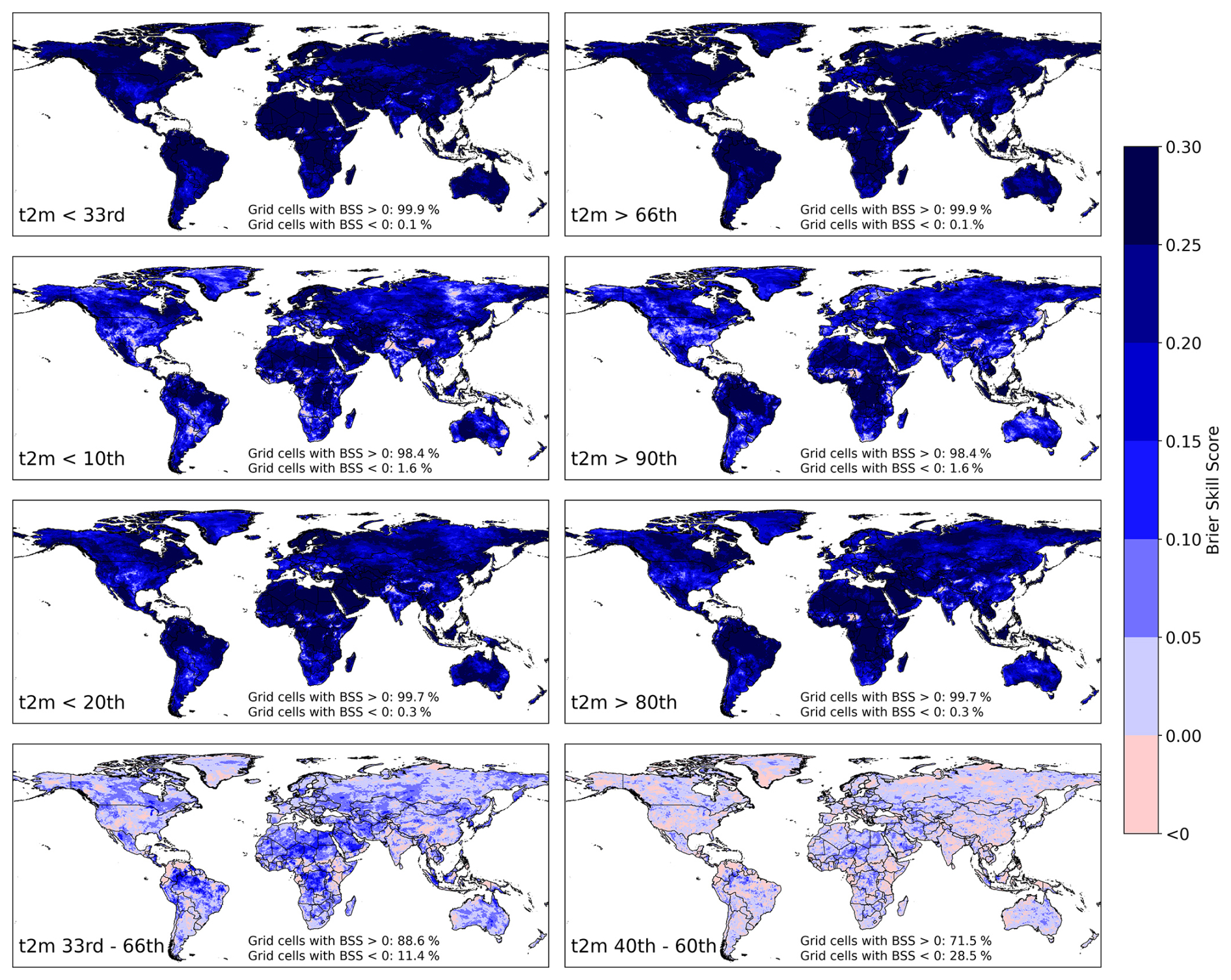
Figure A1 SEAS5-BCSD, Brier Skill Score (BSS) relative to climatology for 2 m-temperature at Lead Month 0. Different percentile thresholds are shown, indicated in the lower-left corner of each panel. Blue colors indicate higher skill than climatology, with darker shades representing better performance.

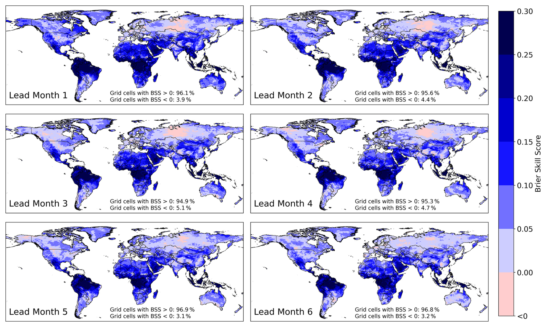
Figure A2 SEAS5-BCSD, Brier Skill Score (BSS) relative to climatology for 2 m-temperature, focusing on dry conditions below the 33rd percentile for Lead Months 1–6. Blue colors indicate higher skill than climatology, with darker shades representing better performance.

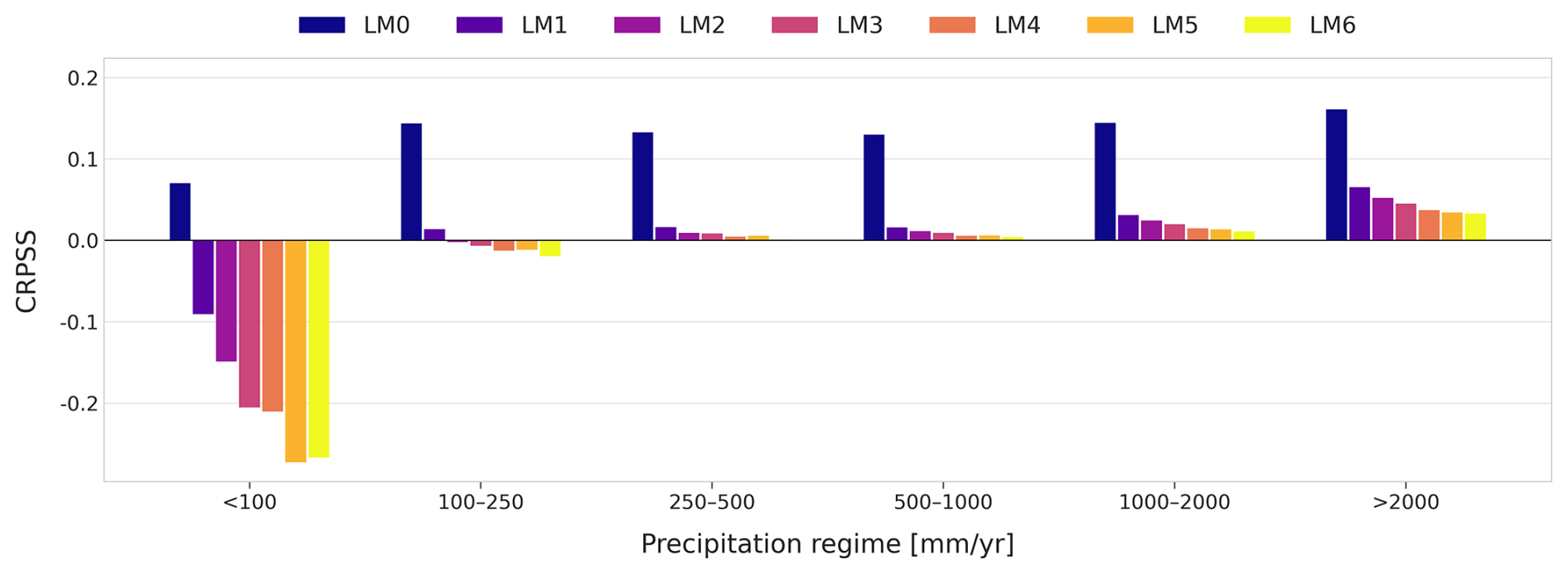
Figure A3 SEAS5-BCSD, yearly mean precipitation sum compared to the Continuous Ranked Probability Skill Score (CRPSS) relative to climatology. The area is grouped by precipitation thresholds into 6 bins, each showing seven lead months.

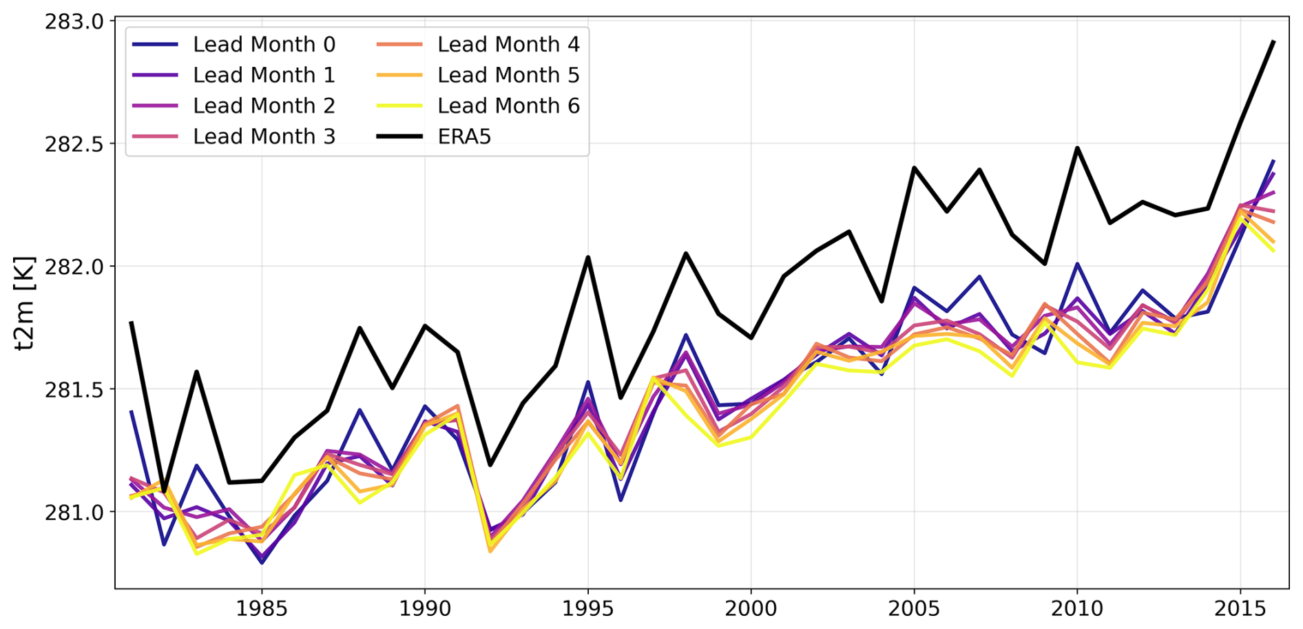
Figure A4 Bias between uncorrected SEAS5 and ERA5 for different lead times. Yearly means across all land masses are shown for the period 1981–2016.

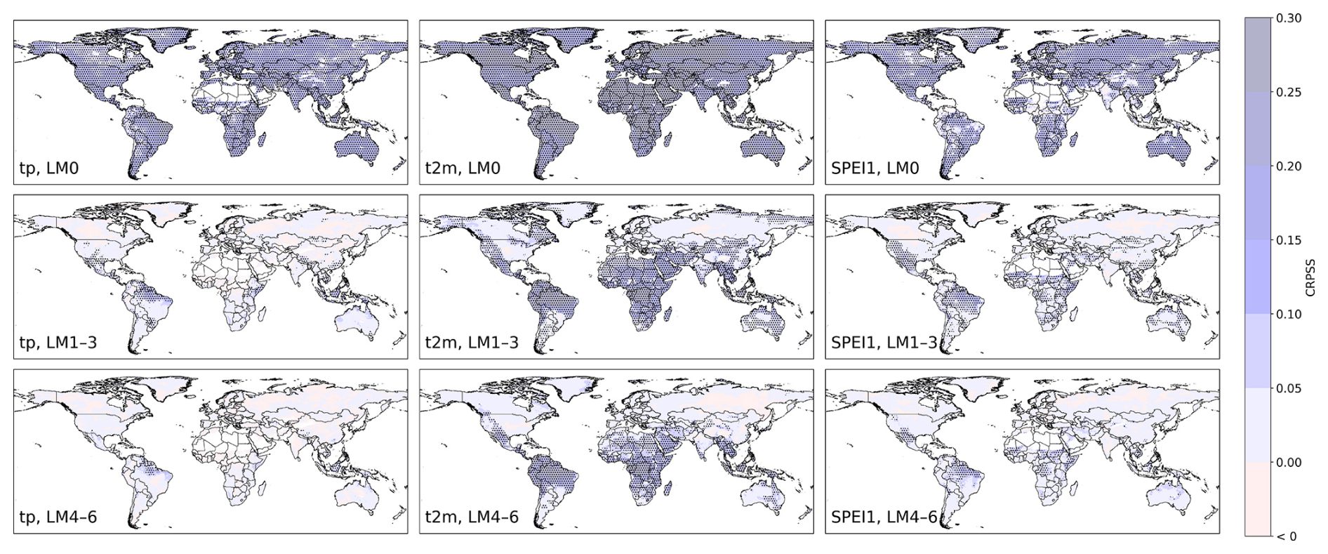
Figure A5 SEAS5-BCSD, Continuous Ranked Probability Skill Score relative to climatology for different lead months (LMs), shown for precipitation (left) and temperature (middle) and SPEI-1 (right). Lead Month 0 (top), Lead Months 1–3 (middle), and Lead Months 4–6 (bottom) are displayed. Dry grid cells are excluded. Hatching indicates grid cells where the lower bootstrap bound exceeds zero (p>0.95).

Table A1 CRPSS of raw SEAS5 forecasts against climatology, averaged per continents.