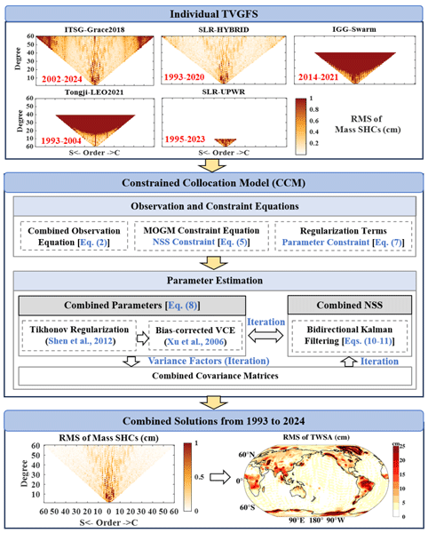
A combination of time-variable gravity field solutions from multi-satellite datasets (1993–2024) via constrained collocation model

Time-variable gravity field solutions from GRACE and GRACE-FO have been successfully applied in hydrological and geophysical studies; however, inter- and intra-mission gaps and limited record length constrain their broader utility. Current approaches involve hydrometeorological-forced machine-learning reconstructions and satellite-tracking-observation combinations; however, the former is constrained by the accuracy and completeness of data inputs, while the latter requires additional filtering due to limited spectral sensitivity, resulting in filtering-dependent solutions. Both approaches neglect covariance information of observation noise and signal, precluding optimal solutions. To address these limitations, this study develops gapless monthly solutions up to degree/order 60 spanning January 1993 to December 2024 using Constrained Collocation Model (CCM) based on Tikhonov regularization, which integrates combination and denoising processes of gravity field solutions without explicit filtering. CCM-based Combined Solutions (CCM-CS) integrates trends, annual and semi-annual variations, and non-seasonal signals from multi-satellite observations (GRACE/-FO, Low Earth Orbit satellites, and Satellite Laser Ranging) without external hydrometeorological inputs, while incorporating covariance matrices of observation errors and combined signals to optimally balance error reduction and signal preservation. Evaluation results indicate that CCM-CS significantly eliminates striping noise and high-degree coefficient noise while effectively preserving low-degree gravity signals (e.g., C20 and C30) and achieving high signal-to-noise ratios. Comparison with three reconstructed products (IGG-SLR-DORIS, RESDCAE, BNML) shows that CCM-CS achieves the lowest sea level budget misclosures, with reductions of 40 %, 2.9 %, and 49 %, respectively. Across 52 major basins, CCM-CS achieves lower water balance errors in 98.1 %, 82.7 %, and 63.5 % of the basins, respectively. For Antarctic and Greenland ice sheet mass changes, CCM-CS closely match IMBIE (Ice Sheet Mass Balance Inter-comparison Exercise) estimates, with trend consistency improvements of 46.8 % and 32.7 % over IGG-SLR-DORIS and 48.6 % and 67.4 % over RESDCAE, respectively. The combined monthly gravity field solutions are available at https://doi.org/10.5281/zenodo.18589507 (Zhang et al., 2026).

1 Introduction

The global mass changes derived from Time-Variable Gravity Field Solutions (TVGFS) are essential for understanding the dynamic interactions among the atmosphere (Han et al., 2004; Sasgen et al., 2024), ocean (Chen et al., 2022; Dobslaw et al., 2020), Terrestrial Water Storage (TWS; Zhang et al., 2023, 2025b; Saemian et al., 2022, 2024; Tourian et al., 2023; Yi et al., 2023), and cryospheric components including ice sheets and mountain glaciers (Zhang et al., 2020; Wang et al., 2024). The Gravity Recovery and Climate Experiment (GRACE), launched in April 2002, and its Follow-On (GRACE/-FO) missions, enabled unprecedented measurements of time-variable gravity fields through ultra-precise inter-satellite K-band ranging, providing monthly temporal resolution and a spatial resolution of approximately 300 km (Tapley et al., 2004; Tapley et al., 2019), which overcomes the limitations of sparse meteorological observation networks and large uncertainties in reanalysis and simulated hydrological models (Rodell and Li, 2023; Saemian, 2024). Long-term and continuous TVGFS facilitate more accurate trend estimation of geophysical and hydrological signals, the dynamic mechanism of climate changes, and the separation of natural and anthropogenic variability (Huang et al., 2021; Zhang et al., 2023; Wen et al., 2025). Furthermore, the success of GRACE/-FO fuels the demand for extending time-variable gravity records from earlier periods (Löcher and Kusche, 2021; Löcher et al., 2025), bridging the one-year gap between GRACE and GRACE-FO (Shen et al., 2021; Wang et al., 2021b), and filling missing monthly solutions during the intra-mission period (Klokočník et al., 2015).

Therefore, numerous studies have utilized multi-source hydrometeorological datasets to reconstruct longer and gapless TWS at global and regional scales based on various Machine Learning (ML) algorithms, such as Convolutional Neural Network (CNN; Mandal et al., 2025; Gentner et al., 2025), Long Short-Term Memory (LSTM; Wang et al., 2021a; Gentner et al., 2025), Random Forest (Jing et al., 2020; Yin et al., 2023; Saemian et al., 2026), and Multiple Linear Regression (MLR; Sun et al., 2020; Saemian et al., 2026). To mitigate substantial performance disparities among different ML algorithms, hybrid algorithms were employed, with globally optimal algorithms selected through comparison with GRACE/-FO observations (Saemian et al., 2026; Mandal et al., 2025). Alternatively, some studies identified regionally optimal ML algorithms for reconstructing TWS across various spatial scales (Li et al., 2021). Additionally, researchers established non-linear statistical models representing hydrological cycle processes to reconstruct long-term global TWS since 1901 using precipitation and temperature datasets (Humphrey and Gudmundsson, 2019), and the statistical models are enhanced by incorporating multiple reanalysis variables and climate factors (Li et al., 2021). Others applied Cyclostationary Empirical Orthogonal Functions (CSEOF) to extract common precipitation and temperature modes for global TWS reconstruction since 1979 (Chandanpurkar et al., 2022).

However, ML-based reconstructions are limited by the accuracy and completeness of hydrometeorological inputs, which always neglect water storage changes from human activities and surface water bodies (e.g., rivers, reservoirs, and lakes), exhibiting substantial uncertainties in data-sparse regions and extreme events (Scanlon et al., 2018, 2019; Rodell and Li, 2023) and poor agreement with GRACE observations in highly human-intervened basins (Scanlon et al., 2018, 2019; Uz et al., 2024). Moreover, hydrometeorological models do not simulate mass variations in polar and oceanic regions (Saemian et al., 2026; Mandal et al., 2025), and some reconstructions fail to recover complete TWS signals by removing trends or seasonal components (Humphrey and Gudmundsson, 2019; Li et al., 2021).

To reconstruct the entire TVGFS encompassing global water mass redistribution, some studies integrated satellite-tracking observations from Satellite Laser Ranging (SLR) (Löcher and Kusche, 2021; Löcher et al., 2025; Chen et al., 2022; Uz et al., 2024) and Doppler Orbitography and Radio-positioning Integrated by Satellites (DORIS) system (Zhong et al., 2021; Chen et al., 2022; Löcher et al., 2025). Specifically, SLR observations were combined with GRACE/-FO Mascon and climate models to develop global mass changes from 1994 to 2021 using a Residual Deep Convolutional Autoencoder (RESDCAE; Uz et al., 2024). Six DORIS orbit observations were combined to derive the Tongji-LEO2021 model up to degree/order (d/o) 40 from 1993 to 2004 (Chen et al., 2022). Moreover, monthly Spherical Harmonic Coefficients (SHCs) from SLR at low degree/order were combined with leading Empirical Orthogonal Functions (EOFs) from GRACE/-FO SHCs up to d/o 60 to reconstruct TVGFS up to d/o 60 from 1993 to 2020 (Löcher and Kusche, 2021), subsequently incorporating DORIS SHCs at low degree/order to derive extended, higher-precision TVGFS from 1984 to 2023 (Löcher et al., 2025). Additionally, Swarm satellites launched in 2013, equipped with dual-frequency GNSS receivers for precise orbit determination, were integrated with SLR to bridge the gap between GRACE and GRACE-FO missions, with relative weights determined using Variance Component Estimation (VCE; Zhong et al., 2021). Alternatively, Forootan et al. (2020) applied Independent Component Analysis (ICA) to combine GRACE spatial modes with Swarm temporal modes, successfully reconstructing water storage changes across 33 global basins during the gap period.

However, additional explicit filtering is required for the existing combination methods due to the limited spectral sensitivity of tracking observations (Löcher and Kusche, 2021; Chen et al., 2022) to suppress high-degree noise and striping artifacts, which inevitably introduce spatial leakage and signal attenuation, particularly affecting short-wavelength signals (Wahr et al., 1998; Kusche, 2007). The choice of filtering parameters and methods introduces subjectivity and inconsistency across different studies, making inter-comparison and validation challenging (Yi et al., 2022; Sharifi et al., 2025). Moreover, principal component methods (e.g., EOF, ICA, CSEOF) used in some combination approaches are limited by the number of leading GRACE modes, constraining spatial resolution, while static spatial modes result in increasing prediction errors and degraded performance away from the GRACE period (Löcher and Kusche, 2021; Chandanpurkar et al., 2022; Löcher et al., 2025). Notably, ML-based reconstructions and existing combination methods neglect the actual covariance information of observations and signals, precluding the optimal solutions.

Therefore, we aim to develop a new time series of monthly gapless gravity field solutions up to d/o 60 from January 1993 to December 2024 that (1) directly integrate multi-satellite observations without relying on external hydrometeorological model inputs, (2) simultaneously perform combination and denoising without requiring additional explicit filtering, and (3) incorporate covariance matrices of both observation errors and signals. Among existing spectral filters, the Improved Parameter Filter (IPF) designed on a Constrained Collocation Model (CCM) demonstrates the optimal performance, exhibiting the highest Signal-to-Noise Ratios (SNRs) and best consistency with Mascon products and independent hydrometeorological datasets (Zhang et al., 2024, 2025a). Hence, the monthly continuous gravity field solutions are derived using the CCM (Zhang et al., 2024, 2025a), which integrates the combination and denoising processes of TVGFS, avoiding signal attenuations and leakage from additional explicit filtering. The Combined Solutions based on CCM (CCM-CS) optimally balances the multi-satellite observation errors and combined time-variable gravity field signals by incorporating covariance matrices of both, ensuring a good performance in noise suppression and signal preservation. Additionally, CCM-CS estimates the combined trends, annual and semi-annual, and Non-Seasonal Signals (NSS), which comprises non-periodic and interannual components and are modeled as a Multi-Order Gauss-Markov (MOGM) process based on temporal correlations (Zhang et al., 2024, 2025a), ensuring more stable combined solutions to mitigate the interference of poor data quality of individual solutions at certain months.

This study combines five types of TVGFS, including ITSG-Grace2018 models at d/o 60 from GRACE/-FO observations (Kvas et al., 2019), Tongji-LEO2021 (Chen et al., 2022) and IGG-Swarm models (Lück et al., 2021) up to d/o 40 from Low Earth Orbit (LEO) satellite observations, IGG-UPWR-SLR models up to d/o 10 from SLR (Galdyn et al., 2024). Since SLR and LEO models are limited to low d/o during pre-GRACE periods, IGG-SLR-HYBRID models (Löcher and Kusche, 2021), derived from combined SLR and GRACE/-FO observations, are also included to ensure a reconstruction up to d/o 60. This paper systematically presents datasets and methodology in Sects. 2 and 3, conducts comprehensive evaluations of CCM-CS against individual solutions and three distinct products at global and basin scales in Sect. 4, and provides conclusions in Sect. 5.2.

2 Datasets

2.1 Multi-Type TVGFS for Combination

Five types of TVGFS are employed for combination, including (1) ITSG-Grace2018 models up to d/o 60 from GRACE/-FO observations spanning April 2002 to December 2020 (Kvas et al., 2019); (2) Tongji-LEO2021 models up to d/o 40 from six types of LEO satellites covering January 1993 to December 2004 (Chen et al., 2022); (3) IGG-Swarm models up to d/o 40 based on a combination of Swarm A, B and C observations from August 2014 to March 2021 (Lück et al., 2021); (4) IGG-UPWR-SLR models up to d/o 10 from SLR spanning February 1995 to November 2023 (Galdyn et al., 2024); and (5) IGG-SLR-HYBRID models up to d/o 60 from combined SLR and GRACE/-FO observations from January 1993 to December 2020 (Löcher and Kusche, 2021). Among these, ITSG-Grace2018 models offer the covariance matrices, while other products (excluding Tongji-LEO2021) provide the formal errors as initial covariance matrices. In contrast, Tongji-LEO2021 lacks precision information, and an identity matrix is adopted as its initial covariance matrix.

During the GRACE/-FO period, the degree-1 coefficients are restored using Technical Note 13, while the C₂₀ and C₃₀ coefficients are replaced with those of Technical Note 14 (TN14; Loomis et al., 2020). For the pre-GRACE and GRACE-gap periods, the degree-1 coefficients are derived from Löcher et al. (2025), whereas the C₂₀ and C₃₀ coefficients remain unmodified. During the entire period, the GIA effect is removed using the ICE6G-D model (Peltier et al., 2018), and the same mean field from the ITSG-Grace2018 models, spanning January 2004 to December 2009, is removed from all TVGFS.

2.2 Previous models for comparisons

Three distinctly reconstructed/combined products are utilized for comparisons:

1. IGG-SLR-DORIS, which only combined satellite-tracking observations from January 1984 to December 2023, including GRACE/-FO, SLR, and DORIS (Löcher et al., 2025);

2. BNML, which only integrated hydrometeorological components from NOAH and CLSM models, covering from January 1979 to December 2022 (Mandal et al., 2025);

3. RESDCAE, which incorporates both satellite-tracking observations from SLR, CSR RL06 mascon, and hydrometeorological variables from ERA5, spanning from January 1994 to December 2020 (Uz et al., 2024).

Other existing reconstructed/combined products are attributed to one of the three types, and thus are not analyzed in this paper.

Notably, IGG-SLR-DORIS is used only for comparison rather than combination because it additionally contains DORIS-related LEO information, which may overlap with the LEO contribution already introduced by Tongji-LEO2021 in our combination framework. Therefore, IGG-SLR-HYBRID is adopted for combination to better isolate the SLR contribution and avoid potential redundancy, while IGG-SLR-DORIS serves as a comparison product with comparable GRACE/-FO, SLR, and LEO-related information.

2.3 Independent Datasets for Verification

In this paper, CCM-CS is evaluated across global and regional Terrestrial Water Storage Anomalies (TWSAs), as well as polar ice sheets. Global-scale TWSAs are assessed using the sea level budget (Eq. S4 in the Supplement; Frederikse et al., 2020), wherein TWSAs are isolated by removing contributions from thermosteric expansion (Δh_therm) and mass changes in the Greenland Ice Sheets (GrIS; Δh_GrIS) and Antarctic Ice Sheet (AIS; Δh_AIS) from total Global Mean Sea Level (GMSL; Δh_GMSL). The GMSL is derived from averaged tide-gauge (Frederikse et al., 2020) and satellite altimetry observations (NASA-SSH, 2024), while other components are obtained from Frederikse et al. (2020), which integrates multiple observational datasets within a probabilistic framework. Regional TWS Changes (TWSC) are evaluated through the water balance equation (Eq. S5; Zhang et al., 2023), incorporating three precipitation, four evapotranspiration, and five runoff datasets from land surface models and in-situ sites, with their temporal and spatial resolutions detailed in Table S1 in the Supplement. Furthermore, AIS and GrIS mass changes derived from CCM-CS are validated against IMBIE (Ice Sheet Mass Balance Inter-comparison Exercise, Shepherd et al., 2021) time series of cumulative mass balance, providing reconciled estimates from altimetry, gravimetry, and input-output methods. During the GRACE period, the average of CSR and JPL RL06 mascon is additionally employed to evaluate TWS from CCM-CS. Comprehensive details of all datasets utilized in this study are summarized in Table S1.

3 Methodology

This section presents the methodology for combining SHCs from multiple TVGFS. The objective is to simultaneously estimate the combined time-invariant parameters (constant, trend, acceleration, annual and semi-annual terms) and time-varying NSS (all residual signals after removing parameter terms, including non-periodic and interannual variations) using a CCM (Sect. 3.1). The temporal correlations of NSS are constrained via a stochastic MOGM process (Sect. 3.2), while the spatial correlations of parameters are incorporated through a regularization matrix (Sect. 3.3), propagated from the spatial expression of parameters. The parameters and NSS are iteratively estimated, where the parameters are obtained using a Tikhonov-regularization constrained collocation criterion, and NSS recursively updated via a bidirectional Kalman Filtering (KF) process (Sect. 3.3). The iteration estimation process is detailed in Sect. 3.4.

3.1 Functional Model

For each TVGFS, SHCs of each d/o are fitted with a harmonic model plus NSS (Zhang et al., 2025a),

$$\begin{array}{}\text{(1)}& \begin{array}{rl}{y}_{k,i}^{lm}& =a_{\mathrm{0},i}^{lm}+a_{\mathrm{1},i}^{lm}\mathrm{\Delta }{t}_k+a_{\mathrm{2},i}^{lm}\mathrm{\Delta }{t}_k^{\mathrm{2}}+a_{\mathrm{3},i}^{lm}\sin \left(\mathrm{2}\mathit{\pi }\mathrm{\Delta }{t}_k\right)\\ & +a_{\mathrm{4},i}^{lm}\cos \left(\mathrm{2}\mathit{\pi }\mathrm{\Delta }{t}_k\right)+a_{\mathrm{5},i}^{lm}\sin \left(\mathrm{4}\mathit{\pi }\mathrm{\Delta }{t}_k\right)\\ & +a_{\mathrm{6},i}^{lm}\cos \left(\mathrm{4}\mathit{\pi }\mathrm{\Delta }{t}_k\right)+s_{k,i}^{lm}+e_{k,i}^{lm}\end{array}\end{array}$$

where $y_{k,i}^{lm}$ and $e_{k,i}^{lm}$ denote the SHCs and corresponding observation errors from the ith model of degree l and order m at month k, with $\mathrm{\Delta }{t}_k=t_k-t_{\mathrm{1}}$ representing the temporal interval between the kth month and the reference period. The coefficients $a_{\mathrm{0},i}^{lm}$, $a_{\mathrm{1},i}^{lm}$, and $a_{\mathrm{2},i}^{lm}$ indicate constant, linear trend, and acceleration; $a_{\mathrm{3},i}^{lm}$, $a_{\mathrm{4},i}^{lm}$ and $a_{\mathrm{5},i}^{lm}$, $a_{\mathrm{6},i}^{lm}$ represent annual and semi-annual oscillations; $s_{k,i}^{lm}$ encompasses the NSS.

By stacking all SHCs of the ith model at kth month into obervation vector y_k,i, and denoting the combined observations from all q_k models as ${\mathit{y}}_k={\left[\begin{array}{cccc}{\mathit{y}}_{k,\mathrm{1}}^T& {\mathit{y}}_{k,\mathrm{2}}^T& \mathrm{\cdots }& {\mathit{y}}_{k,q_k}^T\end{array}\right]}^T$, where q_k accounts for the monthly-varying number of models for combination. Then Eq. (1) is rewritten as,

$$\begin{array}{}\text{(2)}& {\mathit{y}}_k={\mathbf{A}}_k\mathit{x}+{\mathbf{B}}_k{\mathit{s}}_k+{\mathit{e}}_k\end{array}$$

where the design and coefficient matrices are defined as ${\mathbf{A}}_k=\left[\begin{array}{c}{\mathbf{A}}_{k,\mathrm{1}}\\ {\mathbf{A}}_{k,\mathrm{2}}\\ \mathrm{⋮}\\ {\mathbf{A}}_{k,q_k}\end{array}\right]$ and ${\mathbf{B}}_k=\left[\begin{array}{c}{\mathbf{B}}_{k,\mathrm{1}}\\ {\mathbf{B}}_{k,\mathrm{2}}\\ \mathrm{⋮}\\ {\mathbf{B}}_{k,q_k}\end{array}\right]$, with B_k,i and A_k,i ($i=\mathrm{1},\mathrm{\dots },q_k)$ constructed as,

$$\begin{array}{}\text{(3)}& {\displaystyle }{\mathbf{B}}_{k,i}=\left[\begin{array}{cc}{\mathbf{I}}_{M_{k,i}}& {\mathbf{O}}_{M-M_{k,i}}\end{array}\right]\text{(4)}& {\displaystyle }{\mathbf{A}}_{k,i}={\left[\begin{array}{c}\mathrm{1}\\ \mathrm{\Delta }{t}_k\\ \begin{array}{c}\mathrm{\Delta }{t}_k^{\mathrm{2}}\\ \sin \left(\mathrm{2}\mathit{\pi }\mathrm{\Delta }{t}_k\right)\\ \begin{array}{c}\cos \left(\mathrm{2}\mathit{\pi }\mathrm{\Delta }{t}_k\right)\\ \sin \left(\mathrm{4}\mathit{\pi }\mathrm{\Delta }{t}_k\right)\\ \cos \left(\mathrm{4}\mathit{\pi }\mathrm{\Delta }{t}_k\right)\end{array}\end{array}\end{array}\right]}^T\otimes {\mathbf{B}}_{k,i}\end{array}$$

where ⊗ denotes the Kronecker product; ${\mathbf{I}}_{M_{k,i}}$ and ${\mathbf{O}}_{M-M_{k,i}}$ indicate the identity and zero matrices of size $M_{k,i}\times M_{k,i}$ and $(M-M_{k,i})\times (M-M_{k,i})$; M_k,i and M denote the number of monthly SHCs from the q_kthindividual model and targeted combined model. The dimensional difference $(M-M_{k,i})$ arises from the varying quantities of monthly SHCs across different models. x and s_k are the combined parameters and NSS, respectively. The combined observation errors and weights are denoted as ${\mathit{e}}_k={\left[\begin{array}{cccc}{\mathit{e}}_{k,\mathrm{1}}^T& {\mathit{e}}_{k,\mathrm{2}}^T& \mathrm{\cdots }& {\mathit{e}}_{k,q_k}^T\end{array}\right]}^T$ and ${\mathbf{P}}_{e_k}=\mathrm{blkdiag}({\mathbf{P}}_{e_{k,\mathrm{1}}},{\mathbf{P}}_{e_{k,\mathrm{2}}},\mathrm{\cdots },{\mathbf{P}}_{e_k,q_k})$. The covariance matrix ${\mathbf{\Sigma }}_{e_k}={\mathit{\sigma }}_e^{\mathrm{2}}{\mathbf{P}}_{e_k}^{-\mathrm{1}}$, where ${\mathit{\sigma }}_e^{\mathrm{2}}=\mathrm{blkdiag}({\mathit{\sigma }}_{e_{\mathrm{1}}}^{\mathrm{2}}{\mathbf{I}}_{M_{\mathrm{1}}},{\mathit{\sigma }}_{e_{\mathrm{2}}}^{\mathrm{2}}{\mathbf{I}}_{M_{\mathrm{2}}},\mathrm{\cdots },{\mathit{\sigma }}_{e_{q_k}}^{\mathrm{2}}{\mathbf{I}}_{M_{q_k}})$ and ${\mathit{\sigma }}_{e_i}^{\mathrm{2}}$ represents the time-invariant variance factor for ith model, used to balance magnitude disparities across TVGFS.

3.2 Gauss-Markov model for NSS

Since the NSSs s_k vary from month to month, the observation equation after combining various models' SHCs may still be rank-deficient; additional equations or prior information are required to ensure a unique solution. In this paper, we utilize a Gauss-Markov (GM) model to describe the temporal correlations of NSS between r adjacent months (Zhang et al., 2025a),

$$\begin{array}{}\text{(5)}& {\mathit{s}}_k=\sum _{j=k-r}^{k-\mathrm{1}}{\mathbf{\Phi }}_{k,j}{\mathit{s}}_j+{\mathit{w}}_k(k>r)\end{array}$$

where Φ_k,j is a state transition matrix from epoch j to k, and w_k is the normally distributed process noise with zero mean and covariance matrix Q_k. Φ_k,j and Q_k are constructed as follows (Zhang et al., 2025a),

$$\begin{array}{}\text{(6)}& \left\{\begin{array}{l}{\mathbf{\Phi }}_{k,j}=\exp \left(\frac{-\left(t_k-t_j\right)}{{\mathit{\tau }}_s}\right)\otimes {\mathbf{I}}_M\\ {\mathbf{Q}}_k={\mathit{\sigma }}_s^{\mathrm{2}}\left[\mathrm{1}-\sum _{j=k-r}^{k-\mathrm{1}}\exp \left(\frac{-\mathrm{2}\left(t_k-t_j\right)}{{\mathit{\tau }}_s}\right)\right]\otimes {\mathbf{DD}}^T\end{array}\right.\end{array}$$

where, exp(⋅) is the exponential operator; τ_s and ${\mathit{\sigma }}_s^{\mathrm{2}}$ are the correlation time and variance component. D is a diagonal scale matrix with ${\mathbf{D}}_{j,j}=\mathrm{1}/l_j$, where l_j is the degree of jth element of s_k (Siemes et al., 2013), accounting for the noise characteristics.

Compared to other temporal smoothing methods (e.g., moving average, spline smoothing, principal component analysis; Schrama et al., 2007; Crowley and Huang, 2020; Zhou et al., 2023), the GM model provides a simple linear expression that can be easily combined with observation equations and enables efficient recursive estimation via KF. By assuming stochastic process noise, the GM model yields time-dependent prediction covariance matrices, which facilitates integration into the CCM. Additionally, the GM model avoids the empirical selection of smoothing parameters required by other methods, such as moving window size, spline fitting order, or number of principal components.

3.3 Parameter Estimation

The combined parameters are determined based on the cost function of Tikhonov regularization,

$$\begin{array}{}\text{(7)}& \min :\sum _{k=\mathrm{1}}^n{\mathit{e}}_k^T{\mathbf{\Sigma }}_{e_k}^{-\mathrm{1}}{\mathit{e}}_k+\mathit{\alpha }{\mathit{x}}^T\mathbf{R}\mathit{x}\end{array}$$

where n is the total months; α and $\mathbf{R}={\left(\mathbf{DT}{\widehat{\mathit{x}}}_g{\widehat{\mathit{x}}}_g^T{\mathbf{T}}^T{\mathbf{D}}^T\right)}^{-\mathrm{1}}$ (Siemes et al., 2013; Zhang et al., 2025a) are regularization parameter and matrix, with T denoted as the spherical harmonic analysis matrix and x_g defined as the spatial expressions of parameters $\widehat{\mathit{x}}$. Once the initial value of the NSS vector in Eq. (2) is given as ${\widehat{\mathit{s}}}_k^{\left(\mathrm{0}\right)}$, we can derive the regularized solution to parameter vector x based on Eq. (7),

$$\begin{array}{}\text{(8)}& \begin{array}{rl}\widehat{\mathit{x}}& ={\left[\sum _{k=\mathrm{1}}^n{\mathbf{A}}_k^T{\mathbf{\Sigma }}_{e_k}^{-\mathrm{1}}{\mathbf{A}}_k+\mathit{\alpha }\mathbf{R}\right]}^{-\mathrm{1}}\\ & \left[\sum _{k=\mathrm{1}}^n{\mathbf{A}}_k^T{\mathbf{\Sigma }}_{e_k}^{-\mathrm{1}}\left({\mathit{y}}_k-{\mathbf{B}}_k{\widehat{\mathit{s}}}_k^{\left(\mathrm{0}\right)}\right)\right]\end{array}\end{array}$$

The combined NSS vector s_k is estimated based on the following cost function,

$$\begin{array}{}\text{(9)}& \min :\sum _{k=\mathrm{1}}^n{\mathit{e}}_k^T{\mathbf{\Sigma }}_{e_k}^{-\mathrm{1}}{\mathit{e}}_k+{\left({\mathit{s}}_k-{\stackrel{\mathrm{‾}}{\mathit{s}}}_k\right)}^T{\mathbf{\Sigma }}_{{\stackrel{\mathrm{‾}}{s}}_k}^{-\mathrm{1}}\left({\mathit{s}}_k-{\stackrel{\mathrm{‾}}{\mathit{s}}}_k\right)\end{array}$$

where ${\stackrel{\mathrm{‾}}{\mathit{s}}}_k$ and ${\mathbf{\Sigma }}_{{\stackrel{\mathrm{‾}}{s}}_k}$ are predicted NSS and covariance matrix at kth month.

Given ${\mathbf{K}}_k={\mathbf{\Sigma }}_{{\stackrel{\mathrm{‾}}{s}}_k}{\mathbf{B}}_k^T{\left({\mathbf{\Sigma }}_{e_k}+{\mathbf{B}}_k{\mathbf{\Sigma }}_{{\stackrel{\mathrm{‾}}{s}}_k}{\mathbf{B}}_k^T\right)}^{-\mathrm{1}}$ as the gain matrix, ${\widehat{\mathit{s}}}_k$ is estimated using the Kalman Filtering (KF) process (Ji et al., 2013) with the parameters $\widehat{\mathit{x}}$ determined using Eq. (8). The prediction and update steps of the forward KF are shown in Eqs. (10) and (11),

$$\begin{array}{}\text{(10)}& {\displaystyle }\left\{\begin{array}{l}{\stackrel{\mathrm{‾}}{\mathit{s}}}_k=\sum _{j=k-r}^{k-\mathrm{1}}{\mathbf{\Phi }}_{k,j}{\widehat{\mathit{s}}}_j\\ {\mathbf{\Sigma }}_{{\stackrel{\mathrm{‾}}{s}}_k}=\sum _{j=k-r}^{k-\mathrm{1}}{\mathbf{\Phi }}_{k,j}{\mathbf{\Sigma }}_{{\widehat{s}}_k}{\mathbf{\Phi }}_{k,j}^T+{\mathbf{Q}}_k\end{array}\right.\text{(11)}& {\displaystyle }\left\{\begin{array}{l}{\mathbf{K}}_k={\mathbf{\Sigma }}_{{\stackrel{\mathrm{‾}}{s}}_k}{\mathbf{B}}_k^T{\left({\mathbf{\Sigma }}_{e_k}+{\mathbf{B}}_k{\mathbf{\Sigma }}_{{\stackrel{\mathrm{‾}}{s}}_k}{\mathbf{B}}_k^T\right)}^{-\mathrm{1}}\\ {\widehat{\mathit{s}}}_k={\stackrel{\mathrm{‾}}{\mathit{s}}}_k+{\mathbf{K}}_k\left({\mathit{y}}_k-{\mathbf{A}}_k\widehat{\mathit{x}}-{\mathbf{B}}_k{\stackrel{\mathrm{‾}}{\mathit{s}}}_k\right)\\ {\mathbf{\Sigma }}_{{\widehat{s}}_k}=\left({\mathbf{I}}_M-{\mathbf{K}}_k{\mathbf{B}}_k\right){\mathbf{\Sigma }}_{{\stackrel{\mathrm{‾}}{s}}_k}\end{array}\right.\end{array}$$

Initial ${\widehat{\mathit{s}}}_{\mathrm{1}}$ and ${\mathbf{\Sigma }}_{{\widehat{s}}_{\mathrm{1}}}$ are empirically determined as specified in Zhang et al. (2024) and (2025a). To mitigate initial value bias, a backward KF process is also implemented (Ji et al., 2013), which is the time-reversed version of the forward process. The final estimates ${\widehat{\mathit{s}}}_k$ and ${\mathbf{\Sigma }}_{{\widehat{s}}_k}$ are obtained by averaging the bi-directional KF results. After deriving the combined $\widehat{\mathit{x}}$ and ${\widehat{\mathit{s}}}_k$, the combined monthly TVGFS is derived through ${\widehat{\mathit{y}}}_k={\stackrel{\mathrm{‾}}{\mathbf{A}}}_k\widehat{\mathit{x}}+{\widehat{\mathit{s}}}_k$, with ${\overline{\mathbf{A}}}_k={\left[\begin{array}{c}\mathrm{1}\\ \mathrm{\Delta }{t}_k\\ \begin{array}{c}\mathrm{\Delta }{t}_k^{\mathrm{2}}\\ \sin \left(\mathrm{2}\mathit{\pi }\mathrm{\Delta }{t}_k\right)\\ \begin{array}{c}\cos \left(\mathrm{2}\mathit{\pi }\mathrm{\Delta }{t}_k\right)\\ \sin \left(\mathrm{4}\mathit{\pi }\mathrm{\Delta }{t}_k\right)\\ \cos \left(\mathrm{4}\mathit{\pi }\mathrm{\Delta }{t}_k\right)\end{array}\end{array}\end{array}\right]}^T\otimes {\mathbf{I}}_M$.

3.4 Optimal Variable Determination

Since the estimated equations for $\widehat{\mathit{x}}$ and ${\widehat{\mathit{s}}}_k$ in Eqs. (8) and (11) are mutually nested; the estimation process is iteratively conducted. The iteration process involves updating the variance factors ${\mathit{\sigma }}_{e_i}^{\mathrm{2}}$, regularization parameter α, regularization matrix R, and optimal variablesof GM model. Among these, regularization parameter α together with variance factors ${\mathit{\sigma }}_{e_{k,i}}^{\mathrm{2}}$ are iteratively estimated based on the minimum Mean Square Error (MSE; Shen et al., 2012; Ji et al., 2022) and bias-corrected Variance Component Estimation (VCE; Xu et al., 2006). Additionally, the optimal variables of GM model, order r, correlation time τ_s, variance ${\mathit{\sigma }}_s^{\mathrm{2}}$, are searching by minimizing the cost function over predefined search ranges at grid intervals (Ji et al., 2013),

$$\begin{array}{}\text{(12)}& L={\displaystyle \frac{\mathrm{1}}{n}}\sum _{k=\mathrm{1}}^n\log \left(\det \left({\mathbf{C}}_k\right)\right)+{\displaystyle \frac{\mathrm{1}}{n}}\sum _{k=\mathrm{1}}^n{\stackrel{\mathrm{‾}}{\mathit{v}}}_k^T{\mathbf{C}}_k^{-\mathrm{1}}{\stackrel{\mathrm{‾}}{\mathit{v}}}_k\end{array}$$

where ${\stackrel{\mathrm{‾}}{\mathit{v}}}_k={\mathit{y}}_k-{\mathbf{A}}_k\widehat{\mathit{x}}-{\mathbf{B}}_k{\stackrel{\mathrm{‾}}{\mathit{s}}}_k$ reflects the predicted errors, with their covariance matrix ${\mathbf{C}}_k={\mathbf{\Sigma }}_{e_k}+{\mathbf{A}}_k{\mathbf{M}}_{\widehat{\mathit{x}}}{\mathbf{A}}_k^T+{\mathbf{B}}_k{\mathbf{\Sigma }}_{{\stackrel{\mathrm{‾}}{s}}_k}{\mathbf{B}}_k^T$, ${\mathbf{M}}_{\widehat{\mathit{x}}}$ is the MSE of $\widehat{\mathit{x}}$ (Shen et al., 2012; Ji et al., 2022). log(⋅) and det(⋅) are the natural logarithm and determinant operators.

In the implementation, the model order r is searched over integer values from 1 to 6. For each r, τ_s and ${\mathit{\sigma }}_s^{\mathrm{2}}$ are jointly searched within a predefined two-dimensional parameter space. Considering the monthly sampling of TVGFS and the need to avoid overly large process noise that may weaken temporal constraints and introduce high-frequency noise, τ_s is searched from 30 to 360 d with a 30 d interval, while ${\mathit{\sigma }}_s^{\mathrm{2}}$ is searched from 0.001 to 10 cm² with an interval of 0.01 cm².

A concise overview of our study is presented in Fig. 1. The iterative estimation process is detailed in Sect. S2 of the Supplement, with the corresponding flowchart shown in Fig. S5 and core symbols summarized in Table S2. The iteration continues four times until the difference in $\widehat{\mathit{x}}$ between consecutive iterations falls below 1 %. Across various iterations, the regularization parameter α and variance factors ${\mathit{\sigma }}_{e_i}^{\mathrm{2}}$ of ITSG-Grace2018, Tongji-LEO2021, IGG-Swarm, IGG-SLR-HYBRID, and IGG-UPWR-SLR, for j ranging from 1 to 5, are presented in Table 1, along with the optimal r, τ_s, and ${\mathit{\sigma }}_s^{\mathrm{2}}$ for the GM model. Since Tongji-LEO2021 exhibits a larger variance than other solutions (except for IGG-UPWR-SLR), its weight in the combination is inherently small, making the specific choice of its initial weight matrix inconsequential, allowing an identity matrix to approximate with negligible impact (Koch, 1999; Teunissen, 2000).

Table 1 Optimal variables for the combination process across various iterations.

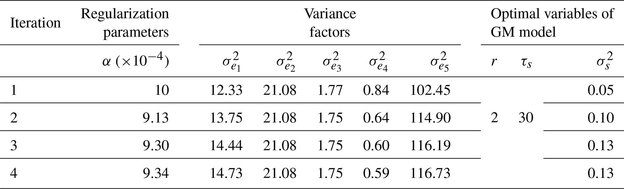
Note: ${\mathit{\sigma }}_{e_i}^{\mathrm{2}}$ for ITSG-Grace2018, Tongji-LEO2021, IGG-Swarm, IGG-SLR-HYBRID, and IGG-UPWR-SLR corresponding to i from 1 to 5.

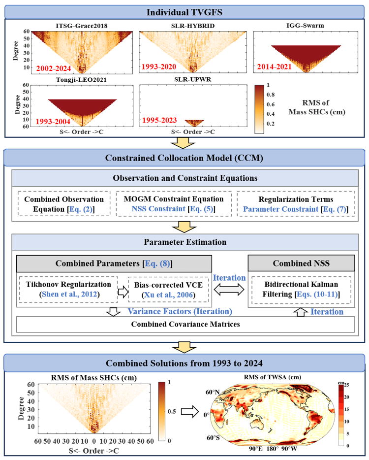
Figure 1 Main procedure for combining TVGFS based on the CCM.

4 Results and Evaluation

4.1 Superiority Over Individual Solutions

Based on the CCM, we develop a gapless time series of gravity field solutions up to d/o 60 from January 1993 to December 2024 through combining monthly TVGFS from ITSG-Grace2018, Tongji-LEO2021, IGG-Swarm, SLR-UPWR, and SLR-HYBRID models. Figure S1 in the Supplement provides the Root Mean Square (RMS) of spatial TWSAs and SHCs across all months, derived from individual solutions and Combined Solutions based on VCE (VCE-CS), which is the most widely used conventional combination method (Jean et al., 2018; Meyer et al., 2019; Zhong et al., 2021). VCE independently combined monthly TVGFS based on their covariance matrices (Meyer et al., 2019). The results indicate that spatial TWSAs and SHCs at high d/o are seriously polluted by striping noise for both individual TVGFS and VCE-CS, requiring additional filtering.

To maintain the consistency with CCM-CS and given the superior performance of the CCM-based filter over all other common spectral filters (Zhang et al., 2024, 2025a), we denoise the individual solutions using the CCM, setting the model number to one as described in Sect. 3.1. The resulting RMS of spatial TWSAs and SHCs across all months are provided in Figs. 2a–e and 3a–e, with those from CCM-CS presented in Figs. 2g and 3g. Additionally, the average SNRs (Eq. S6) and degree powers (Eq. S7) for SHCs are shown in Figs. 2h and 3h–i. The results indicate that CCM-CS exhibits higher SNRs than other individual solutions, effectively removing the serious noise existing in Tongji-LEO2021 (Fig. 2b) and IGG-Swarm (Fig. 2c) solutions, as well as the residual striping noise over oceans in ITSG-Grace2018 (Fig. 2a) and SLR-HYBRID (Fig. 2e) solutions, which originates from spatial leakage and spectral truncation effects (Siemes et al., 2013). In the spectral domain, CCM-CS also demonstrates remarkable noise reduction in IGG-Swarm (Fig. 3c) and Tongji-LEO2021 (Fig. 3d) solutions, while maintaining excellent consistency with the GRACE/-FO solutions from the ITSG-Grace2018 model in terms of low-degree power spectra (Fig. 3i) that primarily contain TVGF signals. Notably, the low-degree power spectra of SLR-HYBRID are significantly lower than those of CCM-CS. These findings underscore that CCM-CS is more effective than individual solutions in simultaneously suppressing noise and preserving signals.

To further demonstrate the superior noise removal efficiency of CCM-CS compared to VCE-CS, the corresponding results are also provided in Figs. 2 and 3. The results indicate that VCE-CS is significantly affected by striping noise from Tongji-LEO2021 and IGG-Swarm, particularly during the gap period of GRACE, resulting in the spatial distribution (Fig. 2f) and spectral power for SHCs between d/o 30 and 40 (Fig. 3f and h), closely resembling Tongji-LEO2021 (Figs. 2b and 3d) and IGG-Swarm solutions (Figs. 2c and 3c). Meanwhile, the low-degree power spectra of VCE-CS are significantly lower than CCM-CS (Fig. 3i). Notably, CCM-CS estimates the combined parameters over a long-term temporal scale and models NSS by utilizing their temporal correlations, which results in more stable solutions and less influence by the absence of GRACE observations, performing significantly higher SNRs (Fig. 2h) and lower noise in SHCs between d/o 30 and 40 compared to VCE-CS (Fig. 3h).

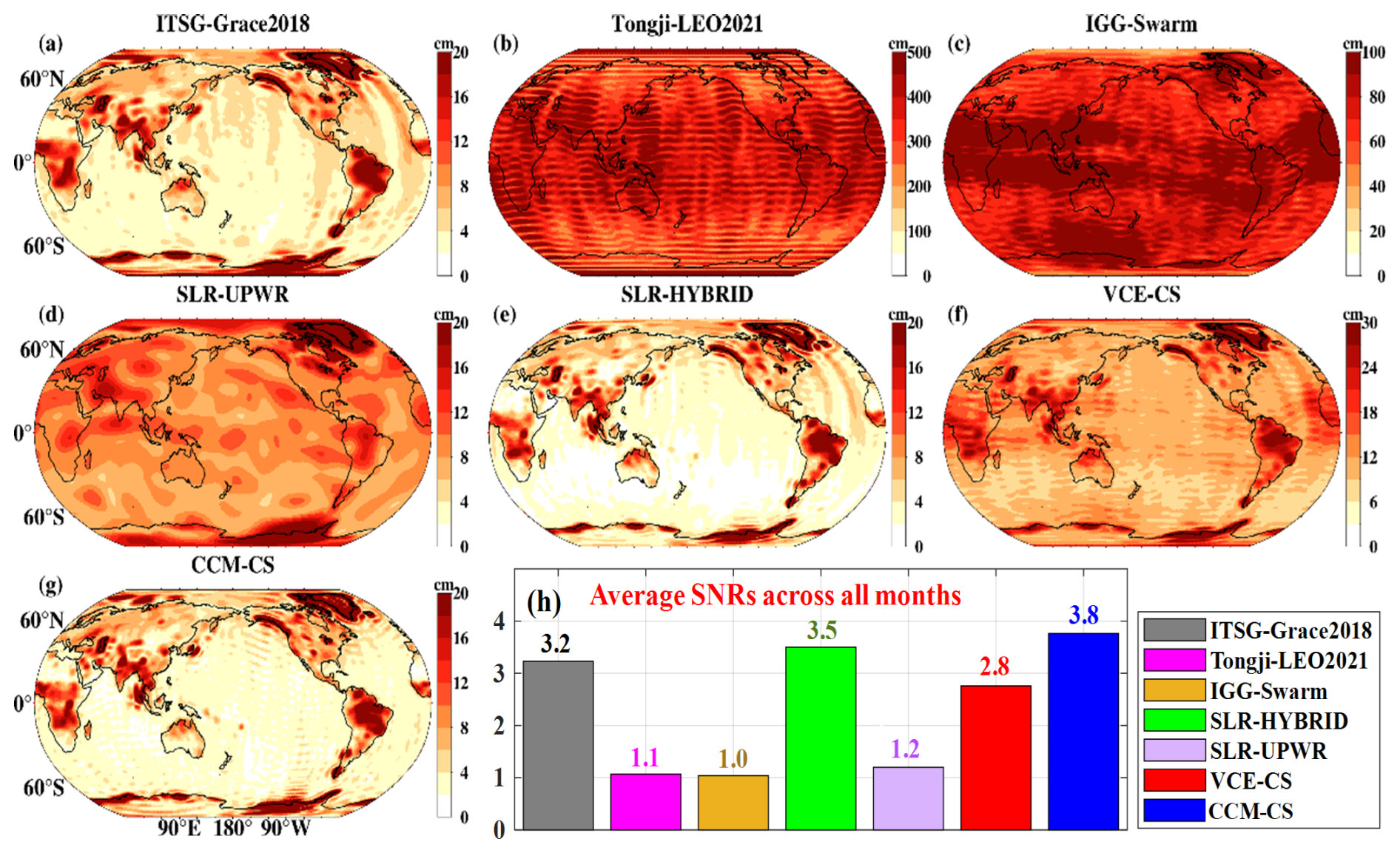
Figure 2 (a–g) RMS of spatial TWSAs and (h) average SNRs from individual and combined solutions over their respective available periods.

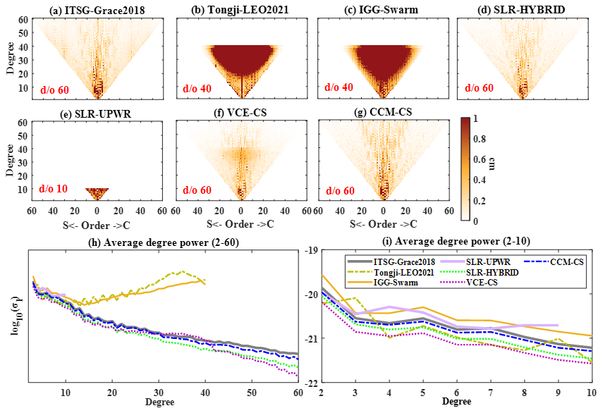
Figure 3 (a–g) RMS of SHCs and average degree power for (h) d/o 2–60 and (i) d/o 2–10 from individual and combined solutions over their respective available periods.

Additionally, the variations ΔC₂₀ and ΔC₃₀ from CCM-CS and individual solutions are provided in Fig. 4a and b, using the official TN14 product as reference. The results demonstrate that CCM-CS effectively reduces the bias of ΔC₂₀ and ΔC₃₀ from individual solutions. Relative to TN14, the Nash-Sutcliffe Efficiency (NSE; Eq. S8; Nash and Sutcliffe, 1970) for ΔC₂₀ and ΔC₃₀ derived from CCM-CS reach 0.96 and 0.98, outperforming ITSG-Grace2018 (0.34), SLR-UPWR (0.93), and SLR-HYBRID (0.88) for ΔC₂₀, and 0.86, 0.14, and 0.94 for ΔC₃₀, respectively. Since the variations ΔC₂₀ and ΔC₃₀ are critical for accurate polar ice sheet mass estimation, we further present the latitude-weighted mass anomaly series of GrIS and AIS derived from CCM-CS and individual solutions up to d/o 60 in Fig. 5a and b, alongside independent IMBIE products that offer reconciled ice sheet mass estimates from altimetry, gravimetry, and the input-output method. Results reveal that the mass anomalies of GrIS and AIS derived from CCM-CS align more closely with IMBIE relative to individual solutions. Notably, the mass anomalies derived from SLR-HYBRID exhibit significant lower signals during GRACE-FO period for GrIS and after 2005 for AIS, while showing anomalously higher signals during 1993 for GrIS and earlier 1995 for AIS, as highlighted by red dashed rectangles. Meanwhile, ITSG-Grace2018 displays substantial anomalous signals due to poor quality of ΔC₂₀ and ΔC₃₀ coefficients. Based on the good performance of ΔC₂₀ and ΔC₃₀ in CCM-CS, particularly vital for the missing months of TN14, we replace ΔC₂₀ and ΔC₃₀ for months with available TN14 product while maintaining no adjustment for the remaining months.

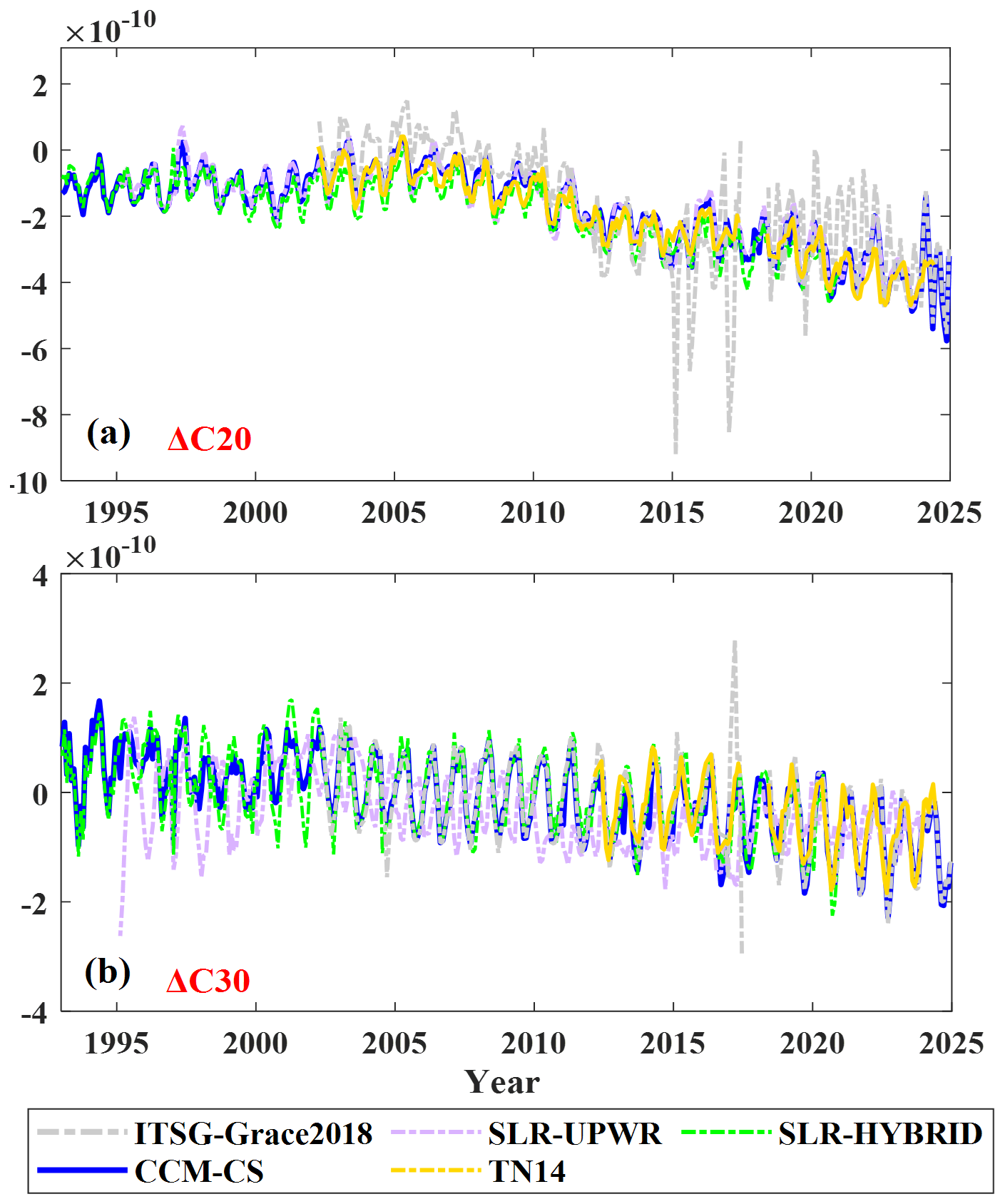
Figure 4 Time series of (a) ΔC₂₀, (b) ΔC₃₀ from CCM-CS and individual solutions, January 1993–December 2024.

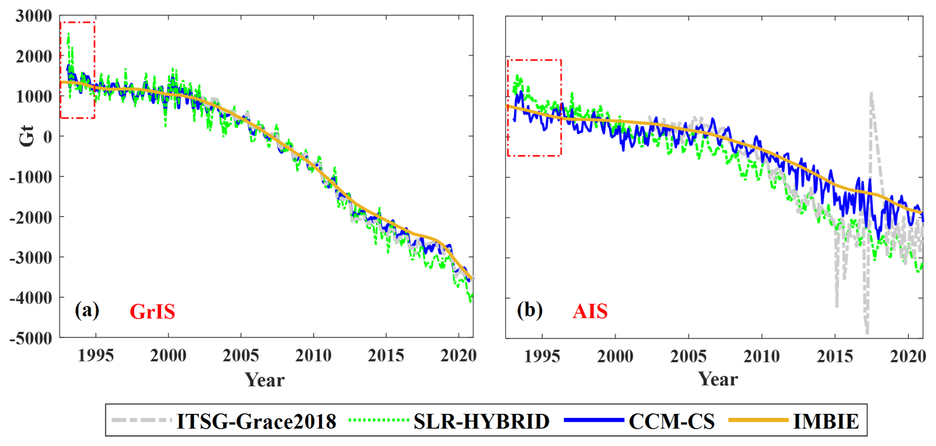
Figure 5 Mass anomalies over (a) GrIS and (b) AIS from CCM-CS and individual solutions, January 1993–December 2020. [Red dashed rectangles indicate solution differences.]

4.2 Comparisons with Previous Models

In this section, CCM-CS is evaluated against three distinct products, including IGG-SLR-DORIS (Löcher et al., 2025), BNML (Mandal et al., 2025), and RESDCAE (Uz et al., 2024), derived from satellite-tracking observations, hydrometeorological models, and a combination of both, spanning from January 1993 to December 2023, January 1993 to December 2024, and January 1994 to December 2020, respectively. IGG-SLR-DORIS is expressed as spherical harmonic coefficients (SHCs) up to d/o 60, while BNML and RESDCAE are presented on 1° spatial grids. Notably, BNML lacks the mass change estimates over Antarctica and Greenland.

4.2.1 Global Terrestrial Water Storage Anomalies

Since BNML and RESDCAE integrate external hydrometeorological datasets and mascon products, their spectral characteristics inherently differ from satellite-only solutions. Therefore, Fig. 6a and b compare the average degree powers and SNRs of CCM-CS with IGG-SLR-DORIS under various filtering strengths. The results reveal that CCM-CS maintains excellent agreement with unfiltered IGG-SLR-DORIS for SHCs below degree 40, while significantly attenuating noise-dominated higher-degree components, yielding substantially higher SNRs. Although Gaussian filtering of IGG-SLR-DORIS reduces high-frequency noise and improves SNRs, it concurrently causes severe attenuation of low-degree SHCs, with signal degradation intensifying as filter radius increases. Nevertheless, regardless of Gaussian filter strength, IGG-SLR-DORIS exhibits inferior SNRs compared to CCM-CS, highlighting the significance of our approach that integrates the combination and denoising processes of TVGFS, thereby circumventing signal attenuation and leakage from additional filtering. To minimize signal bias from serious striping noise while preserving more signal, a 200 km Gaussian filter is applied to IGG-SLR-DORIS in the following analysis.

Additionally, the monthly CCM-CS and IGG-SLR-DORIS solutions are converted into global TWSAs for consistency evaluation. The spatial linear trends from CCM-CS and the reference solutions are shown in Fig. S2. The results show that the TWSA trends from CCM-CS are generally consistent with those from IGG-SLR-DORIS and RESDCAE, particularly over northern India, western North America, southern South America, the Antarctic Peninsula, and the West Antarctic margin, where pronounced decreasing trends are observed. Consistent increasing trends are also found in several regions, including parts of northern Eurasia, eastern North America, central South America, and coastal East Antarctica. In contrast, the hydrometeorological-forced BNML product shows substantially weaker trends over most regions.

To further quantify the differences among various solutions, the NSE values and linear trend differences between CCM-CS and the three reference solutions are presented in Figs. 7 and S3, where the first three rows display metrics relative to RESDCAE, IGG-SLR-DORIS, and BNML, respectively. The results demonstrate that CCM-CS exhibits superior consistency with all three reference solutions compared to their mutual cross-consistencies, as evidenced by higher NSE values and lower linear trend differences. Relative to RESDCAE, the latitude-weighted global NSE and linear trend difference, excluding Greenland and Antarctica, derived from CCM-CS are 0.53 and 0.16 cm yr⁻¹, respectively, outperforming IGG-SLR-DORIS, 0.47 and 0.27 cm yr⁻¹, and BNML, 0.51 and 0.27 cm yr⁻¹. Relative to IGG-SLR-DORIS, CCM-CS attains an NSE of 0.75 and a trend difference of 0.08 cm yr⁻¹, outperforming RESDCAE, 0.43 and 0.27 cm yr⁻¹, and BNML, 0.45 and 0.17 cm yr⁻¹. Relative to BNML, CCM-CS achieves an NSE of 0.46 and a trend difference of 0.10 cm yr⁻¹, whereas IGG-SLR-DORIS, 0.42 and 0.17 cm yr⁻¹, and RESDCAE, 0.24 and 0.27 cm yr⁻¹, exhibit lower consistency.

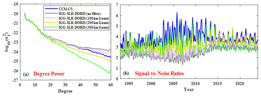
Figure 6 (a) Average degree-powers and (b) SNRs from CCM-CS and IGG-SLR-DORIS under various filtering strengths, January 1993–December 2023.

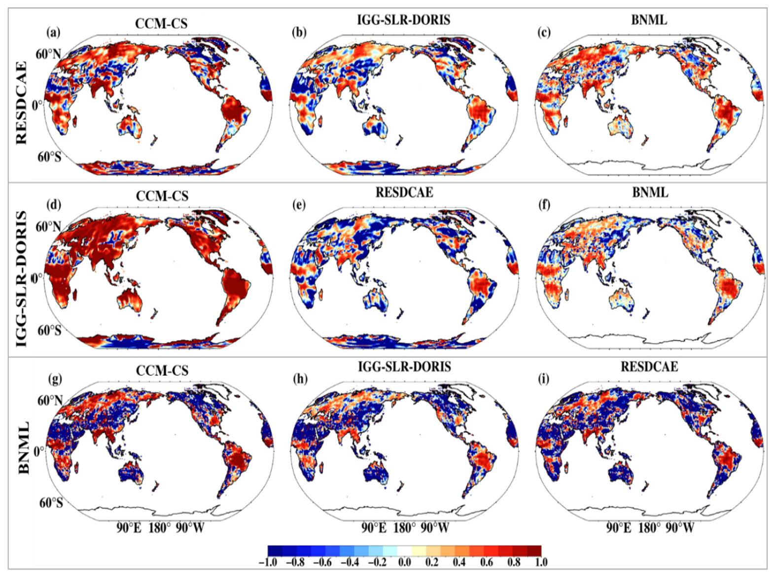
Figure 7 NSE values of global TWSAs from various solutions relative to RESDCAE, IGG-SLR-DORIS, and BNML corresponding to the first to third rows (January 1994–December 2020).

4.2.2 Regional Terrestrial Water Storage Anomalies

To further evaluate the reliability of TWSA signals at the regional scale, we selected 52 major basins with an area exceeding 200 000 km², accounting for substantial uncertainties in TVGFS for small-scale regions (Long et al., 2015), with their spatial distribution illustrated in Fig. S4. Figure 8a–l presents latitude-weighted TWSA series for 12 typical basins derived from various solutions. During the pre-GRACE period, BNML exhibited significant deviations in the Congo, Ganges, Indus, Mississippi, and Yangtze basins, while RESDCAE showed obvious discrepancies in the Mekong, Nile, Yangtze, Zambezi, and Dniepr basins. Additionally, IGG-SLR-DORIS displayed anomalous values due to residual noise (highlighted by dashed ellipses), whereas CCM-CS demonstrated greater robustness compared to other solutions. Furthermore, we computed linear trends and annual amplitudes of TWSA series for all 52 basins (Fig. 8m–n), alongside NSE values relative to mascon products (Fig. 8o), revealing that the linear trends and annual amplitudes from CCM-CS align well with other solutions except for large deviation in the linear trends from RESDCAE, and concurrently, the TWSA series derive from CCM-CS across various basins exhibited significantly higher consistency with mascon products, particularly for TWSA signals from the Congo and Yangtze basins, marked by red dashed rectangles.

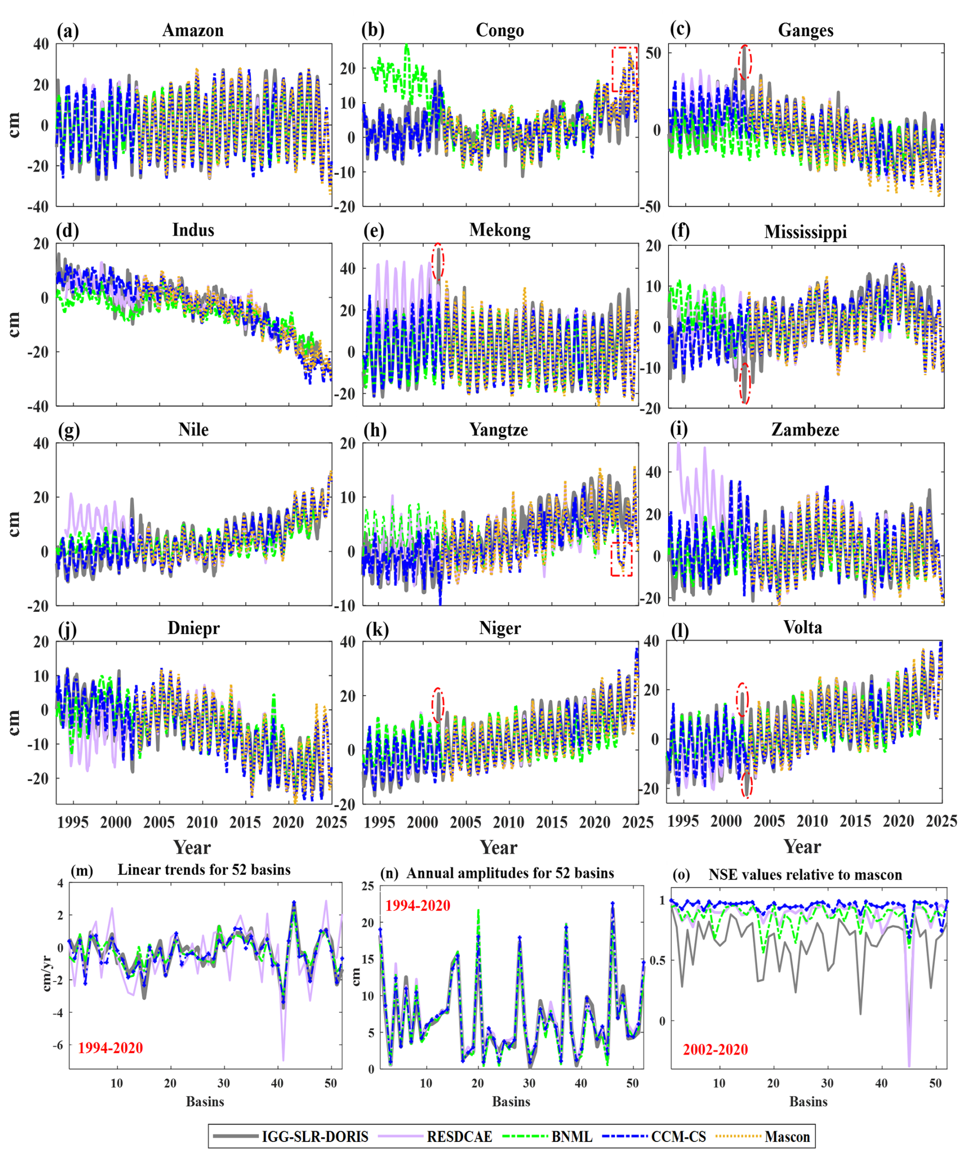
Figure 8 (a–l) Latitude-weighted TWSA series for 12 typical basins (January 1993–December 2024); (m) Linear trends and (n) annual amplitudes of TWSA series for 52 basins (January 1994–December 2020), and (o) their NSE relative to mascon products (April 2002–December 2020). [Red dashed rectangles highlight higher consistencies of CCM-CS with mascon products; red dashed ellipses mark anomalous values from IGG-SLR-DORIS.]

4.3 Evaluation Using Independent Datasets

4.3.1 Sea Level Budget Estimates

Since TWS changes directly affect global mean sea level (GMSL) through land-ocean water exchange, we leveraged this relationship to evaluate the global TWSA from CCM-CS. By removing non-TWS components from GMSL (Eq. S4), including thermosteric expansion (Δh_thermosteric), mass changes of AIS (Δh_AIS), and GrIS (Δh_GrIS), the residual captures the effects of TWS and land glaciers, which are included in TVGFS. The removed components are sourced from Frederikse et al. (2020) at an annual temporal scale, while the GMSL is obtained from the fusion of five altimeter measurements (NASA-SSH, 2024) and tide-gauge (Frederikse et al., 2020). For evaluation, we computed the global TWSA series at the monthly and annual scale (excluding Greenland and Antarctica). At the monthly scale, Fig. 9a displays the latitude-weighted global TWSA series, with RMS Errors (RMSEs) relative to mascon products presented in Fig. 9b, spanning from April 2002 to December 2024. At the annual scale, Fig. 9c presents the global TWSA series, with RMSEs relative to sea level budget estimates shown in Fig. 9d, covering the common period from January 1994 to December 2020. The results demonstrate that global TWSAs derived from CCM-CS exhibit the best agreement with both mascon products and sea level budget estimates, yielding the lowest RMSEs among all solutions. In contrast, BNML displays weaker signal amplitudes during the pre-GRACE period, while IGG-SLR-DORIS shows significant discrepancies during the late GRACE and GRACE-FO periods.

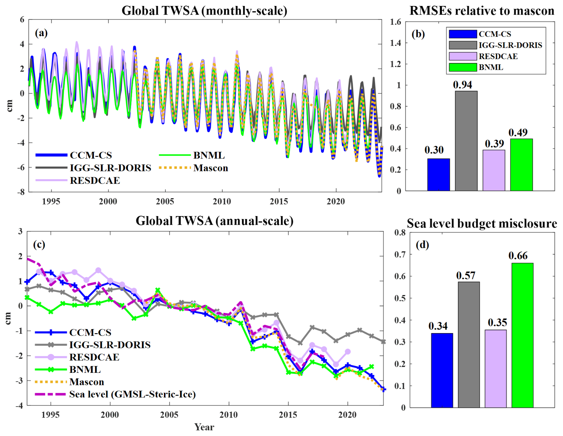
Figure 9 Time series of global TWSAs (excluding Greenland and Antarctic) at (a) monthly and (c) annual temporal scale from various solutions (January 1993–December 2024); (b) RMSEs of monthly TWSA series relative to mascon products (April 2002–December 2020), and (d) sea level budget misclosure from annual TWSA series (January 1994–December 2020).

4.3.2 Water Balance Fluxes

The relationship between TWSCs derived from TVGFS (TWSC_TVGFS) and regional water balance (TWSC_WB) provides a critical way for validating regional TWS variations using independent datasets, where TWSC_TVGFSis computed from the difference in TWSA between adjacent months. TWSC_WB is derived from the residual of precipitation after subtracting runoff and evapotranspiration (Eq. S5). To mitigate large uncertainties in various water fluxes, we utilize three precipitation, four evapotranspiration, and five runoff datasets spanning from January 1993 to December 2019 (detailed in Table S1). Because in-situ runoff observations provide higher local accuracy but sparse and uneven coverage, while gridded simulations offer spatial continuity but larger model uncertainty, the two types of runoff products are fused by ensemble Kalman filter (Evensen, 2003; Clark et al., 2008), as introduced in Sect. S3 of the Supplement. The TWSCs derived from various solutions are denoted as TWSC_CCM, TWSC_SLR-DORIS, TWSC_RESDCAE, and TWSC_BNML.

Subsequently, we compute the RMSEs and Correlation Coefficients (CCs) between TWSC_WB and TWSC_TVGFS at basin-average scales. The RMSEs and CCs for TWSC_CCM relative to other solutions are computed in Fig. 10a–c and d–f. The results indicate that TWSC_CCM exhibits lower RMSEs and higher CCs with TWSC_WB than all other solutions across most basins. To further assess the basin-scale robustness of these improvements, we applied a one-sided paired Wilcoxon signed-rank test at the 95 % significant level (Wilcoxon, 1945; Conover, 1999). TWSC_CCM achieves significantly lower RMSEs than TWSC_SLR-DORIS, TWSC_RESDCAE, and TWSC_BNML in 98.1 %, 82.7 %, and 63.5 % of the 52 basins, respectively, and significantly higher CCs in 88.5 %, 92.3 %, and 71.2 % of the basins.

Further statistical analysis of average RMSEs and CCs between TWSC_TVGFS and TWSC_WB across 52 basins during pre-GRACE (January 1994 to March 2002), GRACE/-FO periods (April 2002 to December 2019), and the entire common period (January 1994 to December 2019) is provided in Fig. 10g and h, revealing that TWSC_CCM exhibits superior performance, especially during the GRACE/-FO period. During the entire common period, TWSC_CCM reduces the RMSEs with TWSC_WB by 4.8 %, 2.5 %, and 1.4 % for TWSC_SLR-DORIS, TWSC_RESDCAE, and TWSC_BNML, while enhancing the corresponding CCs by 9.4 %, 6.1 %, and 2.9 %. Notably, both TWSC_CCM and TWSC_SLR-DORIS incorporate only satellite-tracking observations without hydrometeorological datasets, yet TWSC_CCM demonstrates significantly higher consistency with TWSC_WB compared to TWSC_SLR-DORIS.

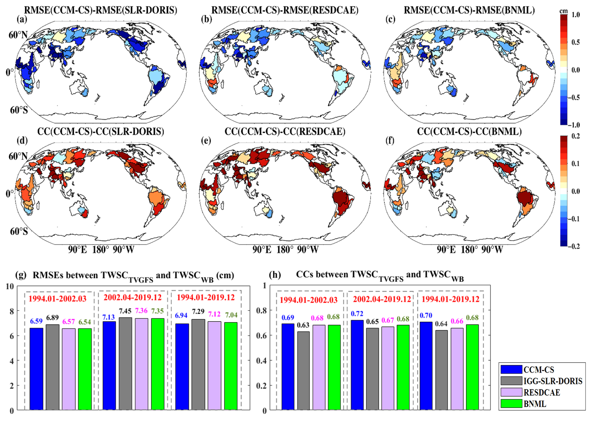
Figure 10 (a–c) RMSEs and (d–f) CCs between TWSC_CCM and TWSC_WB relative to those for TWSC_SLR-DORIS, TWSC_RESDCAE, and TWSC_BNML; and average (g) RMSEs and (h) CCs across 52 basins during pre-GRACE (January 1994 to March 2002), GRACE/-FO periods (April 2002 to December 2019), and the entire common period (January 1994 to December 2019).

4.3.3 Mass Anomalies of AIS and GrIS

Most ML products neglect the reconstructions of AIS and GrIS mass changes, which are incorporated in CCM-CS, IGG-SLR-DORIS, and RESDCAE, making them valuable for reliability evaluation. In Fig. 11a–c and d–f, we present spatial linear trends of Ice Sheet Mass Anomalies (ISMAs) over the Antarctic and Greenland spanning from 1994 to 2020, with Antarctic divided into 18 basins and Greenland into 7 basins, where West Antarctic (WA) comprises basins 3–6 and 17; Antarctic Peninsula (AP) includes basins 1, 2, and 18, and the remaining basins constitute East Antarctic (EA). The results indicate that the trend variations of ISMA estimated from CCM-CS exhibit excellent spatial consistency with those from IGG-SLR-DORIS and RESDCAE. Specifically, ISMA over all basins of AP, basins 3–5 of WA, and basins 10–11 of EA exhibit significantly decreased trends, while those over basins 6, 17 of WA and basins 13–14 of EA show notably enhanced trends. For Greenland, ISMA over Central Greenland (i.e., basin 7) shows enhanced trends, while those for other basins exhibit consistently decreased trends. Notably, the spatial variations of ISMA from CCM-CS exhibit higher consistency with IGG-SLR-DORIS, as RESDCAE underestimates increased ISMA in basin 17 of Antarctica, while overestimating trends in eastern Greenland (basin 7). These discrepancies are attributed to the incorporation of additional climate models into RESDCAE.

Additionally, Fig. 11g and h present latitude-weighted ISMA series over the entire Antarctic and Greenland, incorporating a 300 km region buffer to mitigate coastal signal leakage to the ocean due to spectral filtering and spherical harmonic truncation (Siemes et al., 2013). The ISMA series from IMBIE products serves as a reference, providing reconciled estimates of mass balance from altimetry, gravimetry, and the input-output method. The results indicate that the ISMA series over Antarctica and Greenland derived from CCM-CS shows the highest agreement with IMBIE. For the mass anomalies of AIS, IGG-SLR-DORIS shows significantly overestimated mass loss during the GRACE/-FO period, while RESDCAE exhibits underestimated mass loss during the pre-GRACE period. For the mass anomalies of GrIS, IGG-SLR-DORIS displays underestimated mass loss, while RESDCAE shows overestimated mass loss after 2013. After removing accelerations, annual, and semi-annual terms, CCM-CS estimates linear trends of AIS and GrIS mass anomalies from January 1994 to December 2020 (relative to the middle of study period; Eq. 1) as −99.8 ± 1.8 and −196.6 ± 1.4 Gt yr⁻¹, which significantly better match IMBIE estimates of −96.0 ± 0.5 and −188.7 ± 1.2 Gt yr⁻¹, compared to −103.2 ± 1.8 and −176.9 ± 1.4 Gt yr⁻¹ for IGG-SLR-DORIS, and −88.5 ± 1.1 and −212.8 ± 1.7 Gt yr⁻¹ for RESDCAE, respectively. The consistencies between linear trends of AIS and GrIS mass anomalies estimated from CCM-CS and IMBIE improve by 46.8 % and 32.7 % for IGG-SLR-DORIS, and 48.6 % and 67.4 % for RESDCAE, respectively.

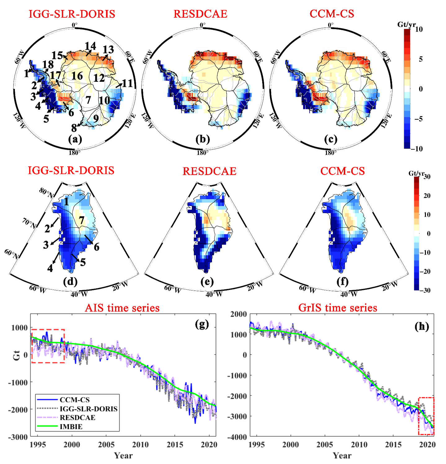
Figure 11 Linear trends of mass anomalies for (a–c) AIS and (d–f) GrIS derived from various solutions; and latitude-weighted time series for (g) AIS and (h) GrIS, January 1994–December 2020. [Red dashed rectangles indicate solution differences. 18 sub-basins of Antarctica are namely (1) I-Ipp, (2) Hp-I, (3) H-Hp, (4) G-H, (5) F-G, (6) Ep-F, (7) E-Ep, (8) Dp-E, (9) D-Dp, (10) Cp-D, (11) C-Cp, (12) B-C, (13) Ap-B, (14) A-Ap, (15) K-A, (16) Jpp-K, (17) J-Jpp, (18) Ipp-J; 7 sub-basins of Greenland are namely (1) NO, (2) NW, (3) CW, (4) SW, (5) SE, (6) CE, (7) NE.]

4.4 Uncertainty Evaluation

The monthly combined TVGFS based on CCM is derived through ${\widehat{\mathit{y}}}_k={\stackrel{\mathrm{‾}}{\mathbf{A}}}_k\widehat{\mathit{x}}+{\widehat{\mathit{s}}}_k$, yielding the monthly covariance matrix ${\mathbf{\Sigma }}_{{\widehat{\mathit{y}}}_k}={\stackrel{\mathrm{‾}}{\mathbf{A}}}_k{\mathbf{\Sigma }}_{\widehat{x}}{\stackrel{\mathrm{‾}}{\mathbf{A}}}_k^T+{\mathbf{\Sigma }}_{{\widehat{s}}_k}$, where ${\mathbf{\Sigma }}_{\widehat{x}}$ is computed via covariance propagation based on Eq. (8) and ${\mathbf{\Sigma }}_{{\widehat{s}}_k}$ is obtained from Eqs. (10) and (11). In the spectral domain, uncertainty of monthly combined solutions is derived from the diagonal elements of covariance matrix ${\mathbf{\Sigma }}_{{\widehat{\mathit{y}}}_k}$, while in the spatial domain, uncertainty of monthly TWSA is propagated from ${\mathbf{\Sigma }}_{{\widehat{s}}_k}$ using the spherical harmonic synthesis matrix. Additionally, the uncertainties of monthly TVGFS from IGG-SLR-DORIS and monthly spatial TWSA from RESDCAE are accessible, with the former propagated from errors of SLR solutions and GRACE/-FO EOFs (Löcher et al., 2025) and the latter computed from standard deviations (Uz et al., 2024). Since the inputs of BNML only include noise-free hydrometeorological datasets, different from those of CCM-CS, its uncertainty is not used for comparison. Across all common months, we compute average uncertainties of TVGFS from CCM-CS and IGG-SLR-DORIS, alongside those of spatial TWSAs from CCM-CS and RESDCAE, through error propagation from monthly uncertainties. The average uncertainties from CCM-CS relative to those from IGG-SLR-DORIS and RESDCAE are provided in Fig. 12a and b. Results demonstrate that CCM-CS exhibits lower uncertainties than IGG-SLR-DORIS solutions, particularly for SHCs at high d/o, while also showing reduced uncertainties relative to RESDCAE over most regions. Average uncertainties across SHCs of all d/o and all spatial TWSA grids are improved by 13.4 % and 14.6 % compared to IGG-SLR-DORIS and RESDCAE solutions, respectively.

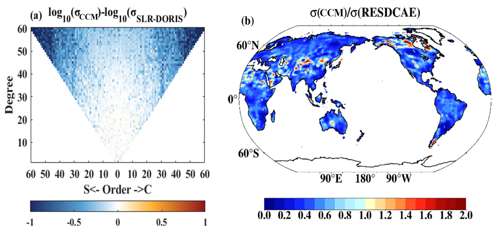
Figure 12 Average uncertainties of (a) SHCs and (b) spatial TWSAs derived from CCM-CS relative to those from IGG-SLR-DORIS (January 1993–December 2023) and RESDCAE (January 1994–December 2020).

5 Data availability

The combined monthly gravity field solutions are available at https://doi.org/10.5281/zenodo.18589507 (Zhang et al., 2026); ITSG-Grace2018 model: https://www.tugraz.at/institute/ifg/downloads/gravity-field-models/itsg-grace2018 (Kvas et al., 2019); Mascon products: https://grace.jpl.nasa.gov/data/get-data/ (last access: 2 July 2026); Five individual TVGFS for combination: https://icgem.gfz.de/hom (last access: 2 July 2026); IMBIE: https://imbie.org/ (last access: 15 March 2021); GMSL from altimeters: https://data.nasa.gov/dataset/ (last access: 23 June 2026); Components of the Sea level budget: Frederikse et al. (2020); Source of Water balance fluxes (Precipitation, evapotranspiration, and runoff) are detailed in the Table S1.

6 Conclusions

In this study, we develop a time series of monthly gapless, explicit-filter-free gravity field solutions up to degree/order (d/o) 60 from January 1993 to December 2024, by estimating combined trends, annual and semi-annual terms, and NSS from five types of TVGFS, which integrates the combination and denoising processes of TVGFS based on the collocation criterion constrained by Tikhonov regularization, thereby mitigating signal attenuation and leakage due to additional filtering employed in conventional combination methods. Covariance matrices of multi-satellite observation errors and combined gravity field signals are incorporated to ensure optimal noise suppression and signal preservation.

Relative to individual solutions, CCM-CS significantly eliminate spatial striping noise and SHC noise at high d/o, while effectively preserving low-degree gravity signals and achieving substantially higher SNRs. Additionally, CCM-CS demonstrates superior consistency with TN14 for low-degree coefficients (C₂₀ and C₃₀), and with IMBIE products for AIS and GrIS mass changes.

Comprehensive evaluations against three distinct products (IGG-SLR-DORIS, RESDCAE, BNML) using independent datasets confirm superior performance at global and regional scales. In the spectral domain, CCM-CS significantly reduces SHC's noise at high d/o, achieving higher SNRs than IGG-SLR-DORIS. For global TWSAs, CCM-CS exhibits the lowest RMSEs against the average of CSR and JPL mascon products and minimal sea level budget misclosures. Regionally, CCM-CS achieves the lowest water balance misclosures with independent hydrometeorological fluxes. For polar ice sheets, CCM-CS estimates mass anomalies over AIS and GrIS closely match IMBIE estimates, with trend consistency improvements of 46.8 % and 32.7 % for IGG-SLR-DORIS and 48.6 % and 67.4 % for RESDCAE, respectively. Furthermore, the average uncertainty of CCM-CS via covariance propagation is reduced by 13.4 % and 14.6 % compared to IGG-SLR-DORIS and RESDCAE, respectively.