Global thermocline vertical velocities: a novel observation based estimate

Vertical velocities at large scales are crucial for understanding ocean dynamics, influencing large-scale circulation and associated biochemical processes, yet their rationale is poorly understood, and their three-dimensional mean distribution and temporal variability are mainly known by models. This paper introduces OLIV3 (Observation-based LInear Vorticity Vertical Velocities), a novel observation-based estimation product of vertical velocities over the global thermocline. This product relies on the geostrophic linear vorticity balance (LVB) applied to ARMOR3D observation-based meridional velocities with ERA5 Ekman pumping vertical velocity as surface boundary condition. It covers the water column over 71 isopycnal levels, with $\mathrm{1}/\mathrm{4}$° horizontal resolution at annual frequency during the 1993–2019 period. Since the geostrophic LVB-derived vertical velocities only capture the geostrophic component of the vertical velocity, their performance is tested using ocean general circulation model (OGCM) data against the total vertical flow. In the thermocline, the LVB accurately reproduces the interannual variability and captures the climatology of the large-scale total vertical flow (horizontal scales larger than 5°) with errors below 50 % across the major ocean gyres. Focusing on surface-thermocline exchanges, one of the most common applications that needs vertical velocities, OGCM results indicates that baroclinic geostrophic vertical velocities are largely more accurate than the classic Ekman pumping proxy at estimating the interannual variability of the total vertical flow in the ocean interior. OLIV3 capability to estimate real ocean vertical velocities is assessed against three reference datasets: two reanalyses and the observation-based product OMEGA3D. A strong spatial and temporal correlation is evidenced between OLIV3 and reanalysis datasets, in contrast to the OMEGA3D, demonstrating even higher correlation than within themselves and supporting the dominance of the geostrophic component of interannual variability of vertical movements. OLIV3 also reconstructs a baroclinic vertical velocity field, consistent with the basin oceanographic concept of Sverdrup balance theory. By building on theoretical advances made since the introduction of Sverdrup and Ekman transport theories, OLIV3 provides a simplified yet physically consistent estimate of large-scale vertical transport. The OLIV3 dataset developed in this study is available at https://doi.org/10.5281/zenodo.16962780 (Cortés-Morales and Lazar, 2025).

1 Introduction

Ocean vertical motion is fundamental to understanding ocean dynamics. These motions serve as critical mechanisms for the exchange of properties between the ocean surface and interior, as well as within the ocean interior. The vertical exchanges encompass essential components such as heat, salinity, CO₂, oxygen, nutrients (silicates, nitrates), and contribute to shape the large-scale thermocline circulation and the Earth's climate regulation (Leach, 1987; Fischer et al., 1989; Klein and Lapeyre, 2009; Mahadevan, 2016; DeVries et al., 2017; Jacox et al., 2018). Upwelling motions are key for sustaining high primary production by supplying nutrients to the euphotic zone, thereby regulating the biological carbon pump (Freilich and Mahadevan, 2019; Uchida et al., 2019; Yang et al., 2021). They also constitute one of the key physical processes of the most productive fisheries regions globally (Pauly and Christensen, 1995). Moreover, the extreme oligotrophy observed in the anticyclonic gyres is attributed to persistent downwelling vertical velocities (Falkowski et al., 1991).

Although the importance of large-scale vertical velocities (w) in ocean dynamics has long been recognised, direct measurements of these motions remain a formidable challenge. This difficulty stems from the extremely weak intensity of the vertical velocity field relative to large-scale horizontal flows. Near the surface, typical magnitudes are on the order of m d⁻¹, decreasing to 0.1 m d⁻¹ within the thermocline and reaching 0.01–0.001 m d⁻¹ at deeper levels in the ocean interior (e.g. Stommel and Arons, 1959; Schott and Stommel, 1978). As a result, the basin-scale ocean's vertical flow remains one of the open questions of physical oceanography. Vertical velocities span nearly four orders of magnitude across spatial and temporal scales. Observations from Lagrangian neutrally buoyant floats, ADCPs (Acoustic Doppler Current Profilers), and the Sentinel V ADCP have captured fine-scale vertical velocities with amplitudes ranging from 10⁻² to 10⁻⁴ m s⁻¹, or about 1000–10 m d⁻¹ (e.g. Bower and Rossby, 1989; Song et al., 1995; Rossby, 2016; D'Asaro et al., 2018; Comby et al., 2022). Such observations are limited to small regions (covering often only a few degrees or less) and energetic features that do not reflect the magnitude of large-scale circulation. Therefore, a combination of observational data and mathematical tools is required to estimate the vertical flow.

Traditional approaches for estimating vertical velocities across different ocean regions were derived from tracer fluxes (e.g. Stommel and Arons, 1959; Robinson and Stommel, 1959; Wyrtki, 1961; Munk, 1966; Wunsch, 1984) or the application of the continuity equation to horizontal current measurements obtained from hydrographic station data (e.g. Stommel and Schott, 1977; Schott and Stommel, 1978; Wyrtki, 1981; Roemmich, 1983) and mooring measurements (e.g. Halpern and Freitag, 1987; Halpern et al., 1989; Weingartner and Weisberg, 1991; Helber and Weisberg, 2001). These early methods provided insight into the small vertical velocities' order of magnitude and upwelling/downwelling patterns of the vertical motions. Vertical velocities have also been inferred from the divergence of horizontal velocity in numerical models (e.g. Madec et al., 2019). This methodology remains impractical for global observation-based applications because of the sparse distribution of direct current measurements. Exceptions to such application to observations are Freeland (2013), which used in situ Argo float observations to estimate w at a single depth in a limited domain of several degrees, assuming zero vertical flow at the surface, and Colin de Verdière and Ollitrault (2016) and Colin de Verdière et al. (2019), which computed vertical velocities from the horizontal divergence of geostrophic velocities inferred from Argo-derived three-dimensional thermohaline fields and float displacements at their parking depth. In the last decade, alternative approaches used isopycnal displacements (Giglio et al., 2013; Christensen et al., 2024), mooring data combined with the momentum and density balances (Sévellec et al., 2015), and biogeochemical tracers (Garcia-Jove et al., 2022). The theoretical frameworks have also expanded to include methods based on the Bernoulli function to infer w (Tailleux, 2023).

A widely used approach for diagnosing vertical velocities is the quasi-geostrophic (QG) omega equation developed initially for the atmosphere by Hoskins et al. (1978). It links the vertical flow to various processes, including the thermal wind imbalance trend, deformation, kinematic deformation, turbulent buoyancy, and turbulent momentum. This diagnostic equation (solvable from a single snapshot) has been used extensively in regional studies (e.g. Tintoré et al., 1991; Pollard and Regier, 1992; Rudnick, 1996; Allen et al., 2001; Buongiorno Nardelli et al., 2001; Gomis et al., 2001; Naveira Garabato et al., 2001; Rodriguez et al., 2001). However, solving the omega equation requires high-resolution 3D fields and well-defined lateral and vertical boundary conditions. The equation was then updated to account for additional physical processes while maintaining the original Hoskins framework (Giordani et al., 2006). It was used to assess mesoscale structures in the Atlantic (Ruiz et al., 2014), Southern (Buongiorno Nardelli et al., 2018) and global oceans (Buongiorno Nardelli, 2020). OMEGA3D (Buongiorno Nardelli et al., 2018; Buongiorno Nardelli, 2020) is the only existing global vertical velocity product based on the omega equation, integrating in situ and satellite-derived fields. Although OMEGA3D provides a valuable benchmark, the absence of observation-based ground truth for w underscores the need for alternative approaches and new products to estimate vertical velocities on global circulation scales.

In contrast to the complexity of the omega equation, the linear vorticity balance (LVB; $\mathit{\beta }v=f\partial w/\partial z$) offers a simple diagnostic tool for estimating the geostrophic vertical flow on the β-plane. When vertically integrated from the surface to a level of no motion, it yields the classic Sverdrup balance, a foundational concept in wind-driven circulation theory (Sverdrup, 1947). The recent study of Cortés-Morales and Lazar (2024) (CM24 in the rest of the paper) has shown in a reference ocean general circulation model (OGCM) simulation in the North Atlantic the capability of the geostrophic LVB-derived vertical velocities to capture accurately the large-scale interannual variability of the vertical velocities, as well as a significant percentage of their time-mean structure, particularly within the thermocline, but also in the intermediate and deep oceans. The LVB's hypothesis breaks down in certain regions. In particular, the approximation is no longer valid near the equator, within the mixed layer, and along western boundary currents, where nonlinear processes are no longer negligible in the vorticity balance.

This work extends the approach developed for the North Atlantic in CM24 to reconstruct observation-based geostrophic vertical velocities globally. It thereby delivers the Observation-based LInear Vorticity Vertical Velocities (OLIV3). The work is structured around the following key objectives: (i) Implementation of the LVB framework using geostrophic meridional velocities from ARMOR3D and Ekman pumping from ERA5 as the surface boundary condition (Sect. 3.1). (ii) Validation and assessment of limitations of the OLIV3 product through an OGCM simulation, treated as a perfect model reference (Sect. 3.2). (iii) Evaluation of the robustness of OLIV3 vertical velocities in reproducing the known large-scale characteristics of the global vertical circulation with existing observation and reanalysis estimates (Sect. 3.3). (iv) Possible physical reasons are proposed to explain why this simplification may or may not be valid in certain regions of the ocean (Sect. 3.4). (v) Comparison with Ekman pumping estimates to identify regions where LVB simplifications can be valid and necessary for describing the ocean interior (Sect. 3.5).

2 Methodology and data

2.1 Revisiting Ekman pumping theory and reconstructing geostrophic vertical velocities

Assuming incompressibility of the total three-dimensional flow implies:

$$\begin{array}{}\text{(1)}& {\displaystyle }{\displaystyle }\mathrm{\nabla }\cdot \mathit{u}=\mathrm{0},\end{array}$$

where the velocity vector is written as $\mathit{u}=(u,v,w)=({\mathit{u}}_{\mathrm{h}},w)$ where u_h denotes the horizontal velocity. The total velocity can be written as the sum of the geostrophic (u_g) and Ekman components (u_Ek):

$$\begin{array}{}\text{(2)}& {\displaystyle }{\displaystyle }\mathrm{\nabla }\cdot {\mathit{u}}_{\mathrm{g}}+\mathrm{\nabla }\cdot {\mathit{u}}_{\text{Ek}}=\mathrm{0}.\end{array}$$

Because the Ekman circulation vanishes below the base of the Ekman layer, the vertical integration of Eq. (2) over the water column can be separated into the Ekman layer, extending from the surface (z=0) to its base (z=D_Ek), and into the ocean interior, extending from the Ekman layer base to a given depth z where we neglect ageostrophic contributions:

$$\begin{array}{}\text{(3)}& {\displaystyle }{\displaystyle }\underset{\text{Ekman Layer}}{\underbrace{\underset{D_{\text{ek}}}{\overset{\mathrm{0}}{\int }}\mathrm{\nabla }\cdot {\mathit{u}}_{\mathrm{g}}\mathrm{d}{z}^{\prime }+\underset{D_{\text{ek}}}{\overset{\mathrm{0}}{\int }}\mathrm{\nabla }\cdot {\mathit{u}}_{\text{Ek}}\mathrm{d}{z}^{\prime }}}+\underset{\text{Ocean Interior}}{\underbrace{\underset{z}{\overset{D_{\text{ek}}}{\int }}\mathrm{\nabla }\cdot {\mathit{u}}_{\mathrm{g}}\mathrm{d}{z}^{\prime }}}=\mathrm{0}.\end{array}$$

The horizontal geostrophic current is calculated from the pressure gradient as

$$\begin{array}{}\text{(4)}& {\displaystyle }{\displaystyle }{u}_{\mathrm{g}}=-{\displaystyle \frac{\mathrm{1}}{{\mathit{\rho }}_{\mathrm{0}}f}}{\displaystyle \frac{\partial p}{\partial y}};v_{\mathrm{g}}={\displaystyle \frac{\mathrm{1}}{{\mathit{\rho }}_{\mathrm{0}}f}}{\displaystyle \frac{\partial p}{\partial x}}.\end{array}$$

Therefore, in a β-plane, the divergence of the horizontal geostrophic flow can be expressed as

$$\begin{array}{}\text{(5)}& {\displaystyle }{\displaystyle }{\mathrm{\nabla }}_{\mathrm{h}}{\mathit{u}}_{\mathrm{h},\mathrm{g}}=-{\displaystyle \frac{\mathit{\beta }{v}_{\mathrm{g}}}{f}}\end{array}$$

assuming f≠0 (Pedlosky, 1996), where f is the Coriolis parameter and β is the meridional gradient of f, without requiring the classical assumption of a linear variation of f across the domain.

The contribution of the Ekman layer in Eq. (3) can be expanded as

$$\begin{array}{ll}{\displaystyle }& {\displaystyle }\underset{D_{\text{ek}}}{\overset{\mathrm{0}}{\int }}-{\displaystyle \frac{\mathit{\beta }{v}_{\mathrm{g}}}{f}}\mathrm{d}{z}^{\prime }+\underset{D_{\text{ek}}}{\overset{\mathrm{0}}{\int }}{\displaystyle \frac{\partial w_{\mathrm{g}}}{\partial z}}\mathrm{d}{z}^{\prime }+\underset{D_{\text{ek}}}{\overset{\mathrm{0}}{\int }}\mathrm{\nabla }\cdot {\mathit{u}}_{\mathrm{h},\text{Ek}}\mathrm{d}{z}^{\prime }\\ \text{(6)}& {\displaystyle }& {\displaystyle }+\underset{D_{\text{ek}}}{\overset{\mathrm{0}}{\int }}{\displaystyle \frac{\partial w_{\text{Ek}}}{\partial z}}\mathrm{d}{z}^{\prime }.\end{array}$$

Evaluating analytically the vertical integrals of the vertical velocity gradients gives

$$\begin{array}{ll}{\displaystyle }& {\displaystyle }\underset{D_{\text{ek}}}{\overset{\mathrm{0}}{\int }}-{\displaystyle \frac{\mathit{\beta }{v}_{\mathrm{g}}}{f}}\mathrm{d}{z}^{\prime }+w_{\mathrm{g}}(z=\mathrm{0})-w_{\mathrm{g}}(z=D_{\text{Ek}})\\ \text{(7)}& {\displaystyle }& {\displaystyle }+\underset{D_{\text{ek}}}{\overset{\mathrm{0}}{\int }}\mathrm{\nabla }\cdot {\mathit{u}}_{\mathrm{h},\text{Ek}}\mathrm{d}{z}^{\prime }+w_{\text{Ek}}(z=\mathrm{0})-w_{\text{Ek}}(z=D_{\text{Ek}}).\end{array}$$

We assume that $w_{\text{Ek}}(z=D_{\text{Ek}})=\mathrm{0}$, as all components of the three-dimensional Ekman flow are dissipated at D_Ek. Furthermore, the Ekman theory relates the Ekman transport,

$$\begin{array}{}\text{(8)}& {\displaystyle }{\displaystyle }{\mathit{U}}_{\mathrm{h},\text{Ek}}=\underset{D_{\text{Ek}}}{\overset{\mathrm{0}}{\int }}{\mathit{u}}_{\mathrm{h},\text{Ek}}\mathrm{d}{z}^{\prime }\end{array}$$

to the wind stress through

$$\begin{array}{}\text{(9)}& {\displaystyle }{\displaystyle }\mathrm{\nabla }\cdot {\mathit{U}}_{\mathrm{h},\text{Ek}}=\mathrm{\nabla }\times \left({\displaystyle \frac{\mathit{\tau }}{{\mathit{\rho }}_{\mathrm{0}}f}}\right),\end{array}$$

where U_h,Ek denotes the horizontal Ekman transport in the Ekman layer, ρ₀ represents the water density at the surface, and τ is the wind stress. Expanding the divergence of the Ekman transport generates

$$\begin{array}{ll}{\displaystyle }\mathrm{\nabla }\cdot {\mathit{U}}_{\mathrm{h},\text{Ek}}& {\displaystyle }=\mathrm{\nabla }\cdot \underset{D_{\text{ek}}}{\overset{\mathrm{0}}{\int }}{\mathit{u}}_{\mathrm{h},\text{Ek}}\mathrm{d}{z}^{\prime }\\ \text{(10)}& {\displaystyle }& {\displaystyle }=\underset{D_{\text{ek}}}{\overset{\mathrm{0}}{\int }}\mathrm{\nabla }\cdot {\mathit{u}}_{\mathrm{h},\text{Ek}}\mathrm{d}{z}^{\prime }-{\mathit{u}}_{\mathrm{h},\text{Ek}}(z=D_{\text{Ek}})\mathrm{\nabla }\cdot D_{\text{Ek}}.\end{array}$$

Consequently,

$$\begin{array}{ll}{\displaystyle }\underset{D_{\text{ek}}}{\overset{\mathrm{0}}{\int }}\mathrm{\nabla }\cdot {\mathit{u}}_{\mathrm{h},\text{Ek}}\mathrm{d}{z}^{\prime }=& {\displaystyle }\mathrm{\nabla }\times \left({\displaystyle \frac{\mathit{\tau }}{{\mathit{\rho }}_{\mathrm{0}}f}}\right)\\ \text{(11)}& {\displaystyle }& {\displaystyle }+{\mathit{u}}_{\mathrm{h},\text{Ek}}(z=D_{\text{Ek}})\mathrm{\nabla }\cdot D_{\text{Ek}}.\end{array}$$

The second term in the right-hand side corresponds to the induction term associated with variations in the Ekman layer depth. This contribution is neglected here, as Ekman velocity is assumed to vanish at D_Ek as mentioned above.

At the sea surface, we impose zero total vertical flow (w_tot),

$$\begin{array}{}\text{(12)}& {\displaystyle }{\displaystyle }{w}_{\text{tot}}(z=\mathrm{0})=\mathrm{0}.\end{array}$$

This condition is exact for the stationary flow of the time-mean state, but it is only an approximation for time-varying flows. In the latter case, this approximation neglects the time derivative of sea surface height, $d\left(\mathit{\eta }\right)/dt$, where η represents the sea surface height relative to the mean state reference surface level. The total vertical velocity is decomposed into geostrophic and ageostrophic components ($w_{\text{tot}}=w_{\mathrm{g}}+w_{\text{ag}}$), where the ageostrophic contribution is assumed, at first order, to be produced by surface wind stress and friction (three-dimensional Ekman flow). Under these assumptions, the surface condition implies:

$$\begin{array}{}\text{(13)}& {\displaystyle }{\displaystyle }{w}_{\mathrm{g}}(z=\mathrm{0})=-w_{\text{Ek}}(z=\mathrm{0}).\end{array}$$

Substituting the Ekman transport (Eq. 9) into Eq. (7) and imposing the surface condition of zero total vertical velocity, the contribution of the Ekman layer in Eq. (3) yields

$$\begin{array}{}\text{(14)}& {\displaystyle }{\displaystyle }\underset{D_{\text{ek}}}{\overset{\mathrm{0}}{\int }}-{\displaystyle \frac{\mathit{\beta }{v}_{\mathrm{g}}}{f}}\mathrm{d}{z}^{\prime }-w_{\mathrm{g}}(z=D_{\text{Ek}})+\mathrm{\nabla }\times \left({\displaystyle \frac{\mathit{\tau }}{{\mathit{\rho }}_{\mathrm{0}}f}}\right).\end{array}$$

In the ocean interior, only the geostrophic currents are not negligible, such that the contribution of the ocean interior to the Eq. (3) can be derived

$$\begin{array}{}\text{(15)}& {\displaystyle }{\displaystyle }\underset{z}{\overset{D_{\text{ek}}}{\int }}-{\displaystyle \frac{\mathit{\beta }{v}_{\mathrm{g}}}{f}}\mathrm{d}{z}^{\prime }+\underset{z}{\overset{D_{\text{ek}}}{\int }}{\displaystyle \frac{\partial w_{\mathrm{g}}}{\partial z}}\mathrm{d}{z}^{\prime }.\end{array}$$

Evaluating the vertical integral of the contribution of the ocean interior to Eq. (3) leads to

$$\begin{array}{}\text{(16)}& {\displaystyle }{\displaystyle }\underset{z}{\overset{D_{\text{ek}}}{\int }}-{\displaystyle \frac{\mathit{\beta }{v}_{\mathrm{g}}}{f}}\mathrm{d}{z}^{\prime }+w_{\mathrm{g}}(z=D_{\text{Ek}})-w_{\mathrm{g}}\left(z\right).\end{array}$$

Combining the Ekman layer (Eq. 14) and ocean interior (Eq. 16) contributions, the terms corresponding to w_g(D_Ek) cancel each other, and the expression for the geostrophic vertical velocity in the ocean interior is obtained

$$\begin{array}{}\text{(17)}& {\displaystyle }{\displaystyle }{w}_{\mathrm{g}}\left(z\right)=\mathrm{\nabla }\times \left({\displaystyle \frac{\mathit{\tau }}{{\mathit{\rho }}_{\mathrm{0}}f}}\right)-\underset{z}{\overset{\mathrm{0}}{\int }}{\displaystyle \frac{\mathit{\beta }{v}_{\mathrm{g}}}{f}}\mathrm{d}{z}^{\prime }.\end{array}$$

In this scenario, the horizontal geostrophic flow is divergent and generates a net geostrophic vertical velocity in the ocean interior. Equation (17) corresponds to the indefinite vertical integral of the LVB applied to the geostrophic flow. While the LVB is an approximation of the vorticity equation valid for large-scale flows, it provides a suitable and well-known foundation for describing the ocean interior flow, as thoroughly described in CM24. As a result of the approximations considered to derive the continuity equation (Eq. 2), discrepancies between the geostrophic vertical velocity and the total vertical velocity are expected, particularly in regions where ageostrophic and nonlinear processes are non-negligible in the ocean interior.

Equation (17) further shows that, although w_g can only be explicitly diagnosed below the Ekman layer, due to the fact that we have defined z below D_Ek in Eq. (3), the magnitude of the vertical flow at the base of the Ekman layer differs from its surface value due to the vertically integrated divergence of the horizontal geostrophic flow within the Ekman layer. At the sea surface or if the geostrophic flow divergence is negligible, the geostrophic vertical velocity is equal to the Ekman pumping. However, CM24 reported a non-negligible contribution of the β-plane geostrophic divergence for an OGCM within the Ekman layer. This effort is consistent with that of Jacox et al. (2018), which, albeit different, similarly emphasises the need to revisit the classical assumption of Ekman theory. Consequently, in this study, Ekman pumping (w_Ek) is adopted as surface boundary condition for the computation of geostrophic vertical velocities.

Table 1 Summary of datasets used for OLIV3 computation and validation.

2.2 Deriving observation-based geostrophic vertical velocities (OLIV3)

To estimate the global ocean vertical velocities from the divergence of the geostrophic flow, meridional geostrophic velocities from ARMOR3D are used in combination with Ekman pumping vertical velocities derived from ERA5 wind stress as boundary condition at the ocean surface. A summary of the main characteristics of the input datasets, including physical variables, cover period, temporal frequency, and horizontal and vertical resolutions, is provided in Table 1.

ARMOR3D dataset (Guinehut et al., 2012; Mulet et al., 2012) integrates satellite-derived and in situ observations. Its derivation first involves the construction of synthetic temperature and salinity fields from altimetric surface level anomaly (SLA; AVISO+, 2015), and sea surface temperature and salinity (SST and SSS) (Reynolds et al., 2007; Droghei et al., 2018) via linear regression method and covariances calculated from historical in situ observations (EN3 dataset (Ingleby and Huddleston, 2007) and Argo floats). The synthetic and observed temperature and salinity profiles are then merged using optimal interpolation (Bretherton et al., 1976). Finally, geostrophic velocities are computed using the thermal wind equation, referenced to the surface geostrophic velocities estimated from the altimetric absolute dynamic topography. The mixed layer depth (MLD) is obtained from the minimum of temperature and density threshold equivalent to a 0.2 °C decrease. ARMOR3D is available at https://doi.org/10.48670/moi-00052.

Ekman pumping vertical velocities are computed from monthly wind stress data provided by ERA5 (Hersbach et al., 2023), the fifth-generation reanalysis of the European Centre for Medium-Range Weather Forecasts (ECMWF). The ERA5 fields are provided at 0.25° horizontal resolution and can be downloaded from the Copernicus Climate Change Service (C3S) Climate Data Store at https://doi.org/10.24381/cds.f17050d7.

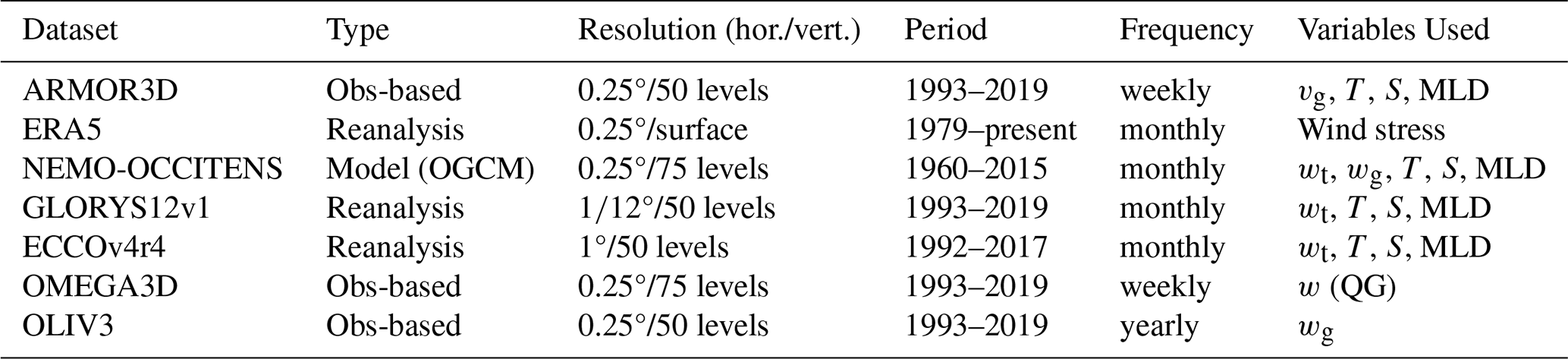
The resulting Observation-based LInear Vorticity Vertical Velocities (OLIV3) product consists of geostrophic vertical velocities derived from ARMOR3D meridional velocities and surface Ekman pumping from ERA5 wind stress, using Eq. (17) over the native ARMOR3D vertical levels and then interpolated over isopycnal levels defined by the neutral density (Jackett et al., 2006) of the ARMOR3D thermohaline field. The product spans the 1993–2019 period, with a horizontal resolution of 0.25° and 71 isopycnal levels. Figure 1 represents the OLIV3 time-mean (1993–2019) vertical velocity at various sigma levels across the tachocline, understood as the upper ocean layer defined by a strong vertical shear in the velocity field (CM24). The product is quality-flagged based on the time-mean relative error and interannual correlation coefficient between w_g and w_tot in the OGCM perfect model test and available at https://doi.org/10.5281/zenodo.16962780 (Cortés-Morales and Lazar, 2025). A low-resolution version, used in the intercomparison test of this study (Sect. 3.3), is available upon request.

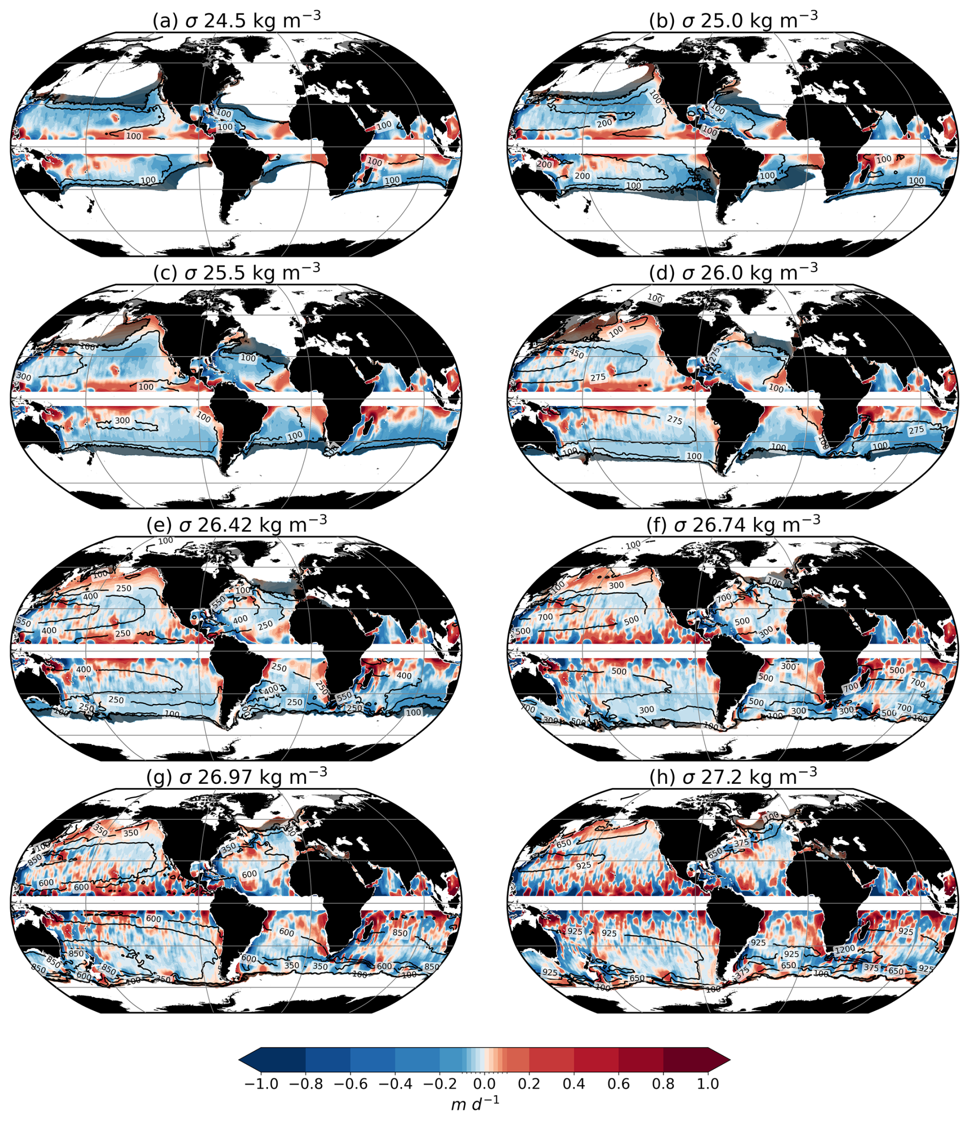
Figure 1 OLIV3 time-mean (1993–2019) vertical velocity at various sigma levels across the tachocline. The field has been smoothed with a 5° running mean. Translucent black shading represents regions within the maximum mixed layer over the study period. The black contour lines represent the depth of the isopycnal surface in m.

2.3 Existing Estimates of Vertical Velocities

To evaluate OLIV3 performance, we compare the vertical velocities with two reanalyses (GLORYS12v1, ECCOv4r4) and an observation-based product (OMEGA3D). To facilitate comparison, the main attributes of the validation product sources are summarised in Table 1.

Following CM24, the reference OGCM simulation for the assessment of validity of the methodology is the Nucleus for European Modelling of the Ocean (NEMO) OGCM OCCITENS run from the OCCIPUT project (Penduff et al., 2014; Bessieres et al., 2017; Madec et al., 2019). This simulation is forced by the DFS5.2 forcing set, using ERA-Interim and ERA40 reanalyses (Dussin et al., 2016). Neutral density field and the isopycnal surfaces were computed for this study using thermohaline and sea surface height fields applied to Jackett et al. (2006) formulation. The MLD provided by the NEMO OCCITENS simulation is computed using a density criterion of 0.01 kg m⁻³ of density change from the surface following the procedure defined by de Boyer Montegut et al. (2004). Outputs from the NEMO OGCM OCCITENS simulation are available upon request (thierry.penduff@cnrs.fr). Geostrophic velocities are derived from the model pressure field (calculated using sea surface height and the hydrostatic equation) using the geostrophic equation via the codes available at https://github.com/meom-group/CDFTOOLS (last access: April 2024).

The GLobal Ocean ReanalYsis and Simulations (GLORYS; Verezemskaya et al., 2021; Lellouche et al., 2021) assimilates via Kalman filter along-track altimeter SLA, satellite SST, sea ice concentration, and in situ temperature and salinity profiles, using NEMO as the model component (Lellouche et al., 2018). The MLD is defined following the same methodology as in the NEMO OGCM simulation. This dataset is hereafter referred to as GLORYS12v1 and accessed at https://tds.mercator-ocean.fr/thredds/glorys12v1/glorys12v1_pgn_monthlymeans.html (last access: April 2024).

The Estimating the Circulation and Climate of the Ocean (ECCO) in its fourth release, version 4 (Forget et al., 2015; Fukumori et al., 2018) employs a 4D-VAR assimilation scheme, integrating satellite altimetry, in situ temperature and salinity profiles from Argo, satellite sea surface salinity and temperature, and ocean bottom pressure, together with the MIT general circulation model (Adcroft et al., 2004). The MLD is defined following the procedure developed by Kara et al. (2000, 2003), which find that the optimal estimated of turbulent mixing penetration is obtained with a mixed layer depth definition of ΔT=0.8 °C. This reanalysis, hereafter referred to as ECCOv4r4, is available at https://www.ecco-group.org/products-ECCO-V4r4.htm (last access: April 2024).

Finally, OMEGA3D is an observation-based global estimate of vertical velocities derived from the QG omega equation (Buongiorno Nardelli et al., 2018; Buongiorno Nardelli, 2020). It is based on ARMOR3D thermohaline field and geostrophic velocities, and ERA-Interim (Dee et al., 2011) surface air-sea fluxes. OMEGA3D is available at https://doi.org/10.48670/moi-00053.

2.4 Validation methodology

Validating OLIV3 with observational data is problematic due to the lack of a ground truth for large-scale vertical velocities. Here, the performance of OLIV3 relies on the consistency across existing w estimates: GLORYS12v1, ECCOv4r4 and OMEGA3D. The intercomparison is conducted on a common spatiotemporal resolution: annual means at 5° horizontal resolution and isopycnal levels. This choice reduces vertical grid and thermohaline structure differences. It also allows to focus on large-scale dynamics, which are better resolved by the LVB framework (CM24). The isopycnal levels are defined by the neutral density (Jackett et al., 2006) of each dataset. For the OLIV3 and OMEGA3D datasets, the thermohaline field used to interpolate w onto isopycnal levels is ARMOR3D, since the velocity field was constructed using it (Buongiorno Nardelli, 2020). Diagnostics are computed over the overlapping 23-year period (1993–2015) and include the time-mean horizontal pattern, the time-mean vertical gradient between isopycnals, the interannual variance and correlation coefficient (R). Regions within the equator band (5° S/N) are excluded as the geostrophic equation cannot be solved at these latitudes.

3 Results and discussion

3.1 Observation-based linear vorticity vertical velocities (OLIV3)

Twenty-seven-year mean geostrophic vertical velocities (w_g) stemming from the OLIV3 product at σ26 isopycnal surface are presented in Fig. 2a. This isopycnal level was chosen to assess the vertical velocity estimates across most of the extension of the global subtropical gyres, while maintaining a focus on thermocline dynamics, where the LVB framework performs best (see CM24 for the North Atlantic Ocean). The geostrophic vertical velocity field (OLIV3) within the tachocline reproduces the well-known wind-driven circulation features represented by Ekman pumping (Fig. 2b), generally with upwelling at tropical latitudes and downwelling at the subtropics. This emphasises the role of wind-driven divergence as the primary driver of vertical flow within the upper ocean (e.g. Huang and Russell, 1994; Liang et al., 2017). The Pacific and Atlantic eastern tropical upwelling systems that continue along the eastern coast up to subtropical latitudes are associated with maximum positive values near the coast around 0.2 m d⁻¹ (Aristegui et al., 2009). The anticyclonic circulation of subtropical systems is characterised by negative w (downwelling) with maximum values found along western boundaries. This pattern differs from the agreement among reanalyses about upwelling in most of the western boundary current systems, in particular the Gulf Stream and the Kuroshio Current (Liao et al., 2022). In the Gulf Stream case, this poor agreement with reanalyses aligns with the lack of confidence in the LVB as an estimator of the vertical flow, as we already demonstrated in the Atlantic Ocean. Outside the Northern Hemisphere subtropical band, some upwelling occurs over the extension of the Gulf Stream and Kuroshio systems, which can be explained by Ekman pumping (Qiu and Huang, 1995).

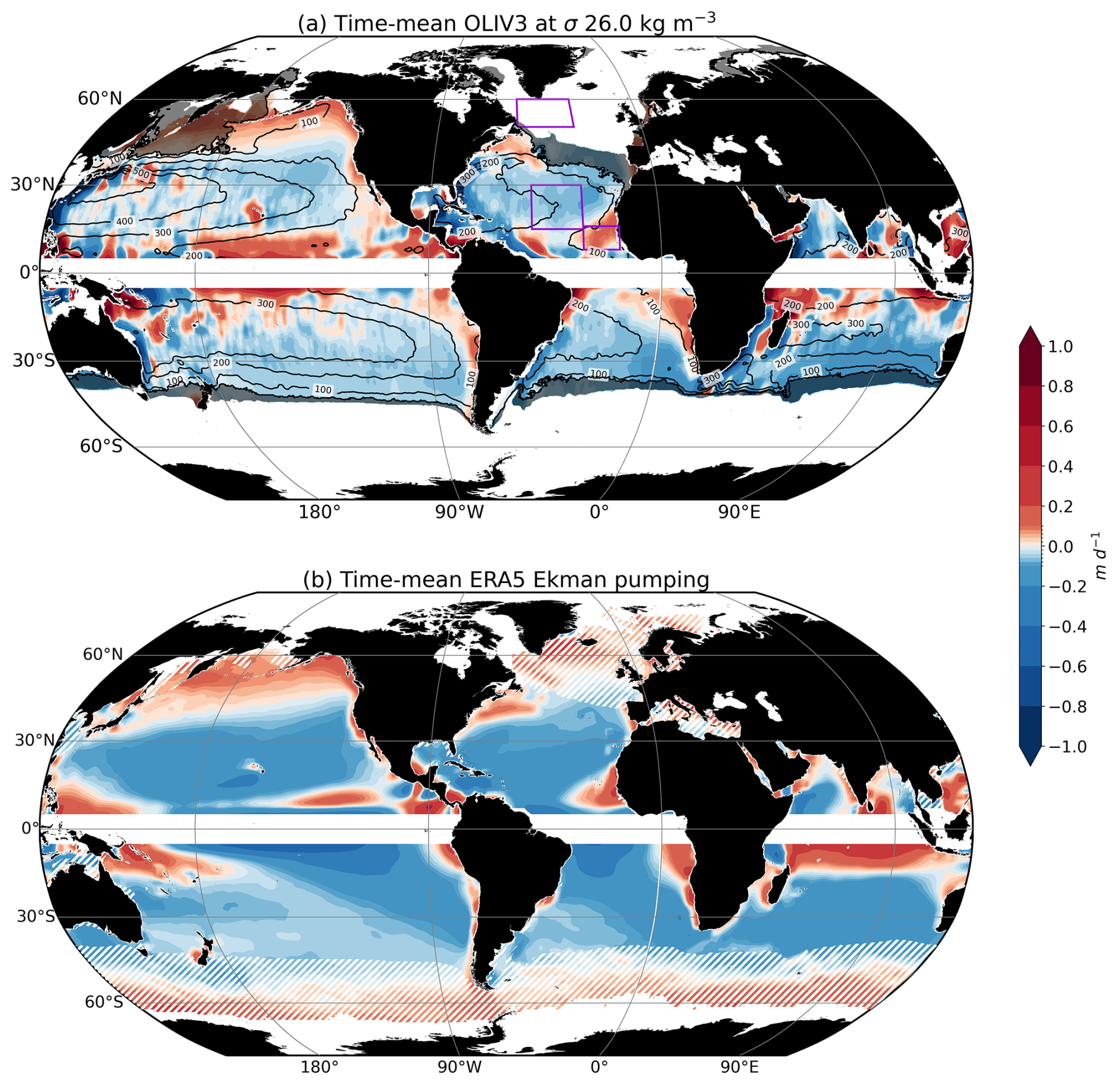
Figure 2 (a) OLIV3 time-mean (1993–2019) vertical velocity at σ26. The field has been smoothed with a 5° running mean. Translucent black shading represents regions within the maximum mixed layer over the study period. The black contour lines represent the depth of the isopycnal surface in meters. Purple rectangles indicate the average regions for Fig. 3. (b) Time-mean Ekman pumping from ERA5. The field has been smoothed with a 5° running mean. White hatching masks the regions above σ26 for comparison purposes.

To analyse the temporal and vertical variability of the vertical velocity estimates, Fig. 3 shows regionally averaged w_g as a function of isopycnal level and year for three distinct regions in the North Atlantic Ocean: the eastern tropical, subtropical and subpolar gyres (purple regions in Fig. 2a). The bottom of the layer was selected as the level where the estimates' climatology changes sign. Figure 3 evidences that the direction of geostrophic vertical velocity estimates maintains their sign throughout most of the layer's thickness. Before reaching this depth, the annual velocities reduce in amplitude, supporting the baroclinic nature of vertical flow found in the North Atlantic tachocline (CM24). This behaviour is consistent with the requirement of a level of no motion at depth to satisfy the Sverdrup balance (Thomas et al., 2014).

Figure 3 Regionally averaged vertical velocity estimates from OLIV3 as a function of isopycnal surface and year for three subregions in the North Atlantic Ocean (NATL): (top) Tropical Gyre (30–16° W, 8–16° N), (middle) Subtropical Gyre (50–30° W, 15–30° N), and (bottom) Subpolar Gyre (55–30° W, 50–60° N). For each region, the first isopycnal level corresponds to the shallowest level that does not intersect the sea surface. Contours of vertical velocities have been included for readability (m d⁻¹).

The velocity sign remains unchanged over time in the three regions (Fig. 3), but temporal variability is evident across them. Weaker upwelling events in the North Atlantic Tropical Gyre (e.g. 1995, 2001, 2005, and 2010 in the top panel of Fig. 3) seem associated with the negative North Atlantic Oscillation (NAO) phases shown by Pinto and Raible (2012) and Roch et al. (2024), while positive NAO phases correspond to stronger upwelling. This suggests that the variability of the eastern tropical gyre is modulated by the phase of the NAO. Interestingly, the magnitude of the oceanic response does not reflect the NAO intensity presented in the references above. Focusing on the subtropical gyre (central panel in Fig. 3), maximum downwelling events do not correlate with the NAO index as clearly as the tropical upwelling does. The atmospheric changes modify both the intensity of the downwelling and the location of the subduction maximum (Pinto and Raible, 2012). Therefore, the out-of-phase relationship between subtropical vertical flow variability and the NAO index may suggest that this region does not fully reproduce the gyre interannual variability. However, other components can influence the variability of the region as the NAO is not the sole contributor to atmospheric forcing variability (Zhao and Johns, 2014). In the subpolar gyre (bottom panel in Fig. 3), oscillations in upwelling amplitude exhibit a periodicity of approximately 5 years, with particularly strong positive velocity events during 2002–2003, 2007, and 2009. These features align with observed changes in the subpolar gyre from satellite altimetry (Foukal and Lozier, 2017) and volume transport estimates of the East Greenland Current (Daniault et al., 2011). These findings suggest that OLIV3, while capturing the baroclinic nature of the vertical velocity field in the tachocline, is also capable of transmitting some of the surface interannual signal into the ocean interior.

3.2 Linear vorticity balance framework in a perfect model test

The vertical flow computed by applying Eq. (17) to the ARMOR3D dataset represents the geostrophic component only. Therefore, before comparing OLIV3 with estimates of the total vertical flow, the limitations of this formulation are evaluated using an OGCM simulation, considered as a “perfect model test”. In this approach, w_g is computed from the model output meridional geostrophic velocity (v_g) and wind stress, following Eq. (17). This global-scale analysis extends the regional assessment conducted by CM24 for the North Atlantic Ocean. To evaluate the ability of the geostrophic component to represent the spatiotemporal variability of the total vertical flow, we examine three diagnostics: the absolute relative error between the time-mean geostrophic vertical velocity (w_g) and the total vertical velocity (w_tot) at σ 26, their interannual correlation coefficient at σ26, as well as the relative error in the time-mean vertical gradient between the bottom of the mixed layer (MLD) and σ27 computed using an OGCM simulation over the period 1993–2015 (Fig. 4). The time-mean vertical gradient of vertical velocities between the base of the maximum mixed layer and σ27 has been normalised by the distance (in meters) between these isopycnal levels, as follows:

$$\begin{array}{}\text{(18)}& {\displaystyle }{\displaystyle }{\mathrm{\Delta }}_{z}w={\displaystyle \frac{\left|w_{\mathit{\sigma }\mathrm{27}}\right|-\left|w_{\mathit{\sigma }\text{MLD}}\right|}{|z_{\mathit{\sigma }\mathrm{27}}-z_{\mathit{\sigma }\text{MLD}}|}}.\end{array}$$

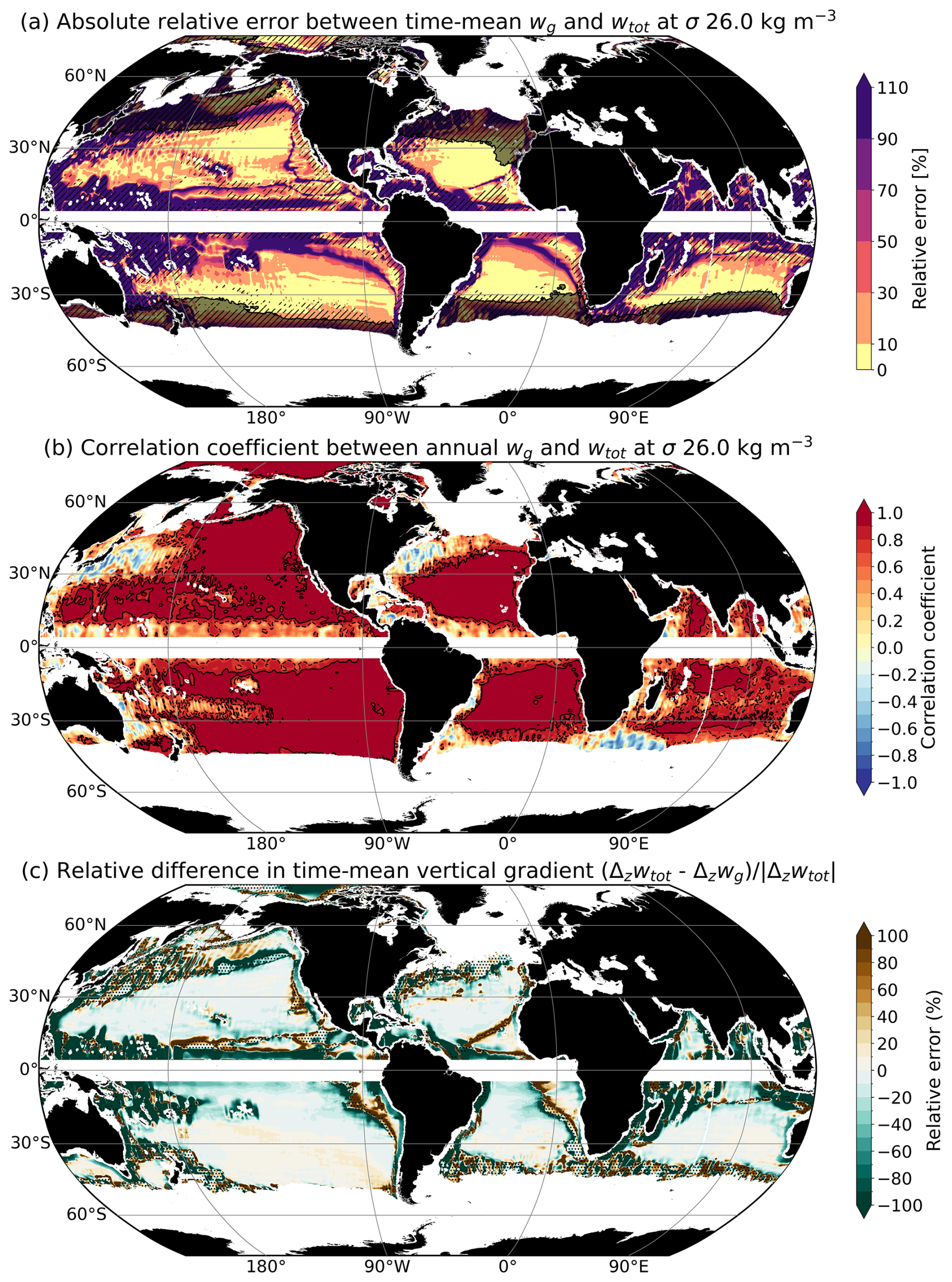
Figure 4 Assessment of OGCM geostrophic vertical velocity (w_g) estimate against the OGCM total vertical velocity (w_tot). (a) Absolute relative error between means of geostrophic vertical velocity and total vertical velocity at σ26 isopycnal surface. Translucent black shading represents regions within the maximum mixed layer over the study period, and hatching delimits the areas where the LVB does not hold (relative error >10 %). (b) Correlation coefficient between the annual geostrophic vertical velocity and total vertical velocity at σ26 isopycnal surface. Black contours indicate correlation coefficients of 0.7 (dashed) and 0.9 (solid). (c) Relative difference in vertical gradient of total and geostrophic time-mean vertical velocity (Δw_tot and Δ_zw_g respectively) between the mixed layer base and σ27, computed as ${\mathrm{\Delta }}_{z}w=\left(\right|w_{\mathit{\sigma }\mathrm{27}}|-|w_{\mathit{\sigma }\text{MLD}}\left|\right)/\left(\right|z_{\mathit{\sigma }\mathrm{27}}-z_{\mathit{\sigma }\text{MLD}}\left|\right)$ normalised by the magnitude of the vertical gradient of the total vertical velocity. Only the regions with MLD shallower than σ27 are considered for this analysis. Dotted (no dotted) areas indicate regions where total vertical velocities display a positive (negative) vertical gradient, meaning increasing (decreasing) magnitude with depth.

Negative values indicate a decrease in magnitude with depth, while positive values indicate an increase. The velocity fields were smoothed with a 5° running mean to retain large-scale structures that LVB can describe (CM24).

As shown in CM24 for the North Atlantic, w_g succeeds in estimating w_tot over most parts of the basins. Figure 4a shows that values are accurate, with a relative error below 50 %, across most of the global tropical and subtropical gyres (yellow, orange and red regions), as well as the eastern part of the subpolar Pacific gyre and the Arctic Beaufort gyre. This result shows that the geostrophic vertical velocity field generally reproduces the spatial structure and amplitude of the thermocline vertical flow within the major gyres in the model simulation, suggesting that a similar behaviour may occur in the real ocean.

Relative errors exceed 50 % in several regions. These include the intergyres bands, where vertical velocities change sign, as well as larger regions of intense current systems, such as the Gulf Stream and its north-eastward extension, the Brazil–Malvinas Current, the Kuroshio Current, the Eastern Australia Current and the Algulhas Current (see locations in Barceló-Llull et al., 2025). High relative errors are also found in regions dominated by strong zonal flows, like the deep tropics, such as the Equatorial Currents and Countercurrents, but also open ocean poleward extensions of western boundary currents like the North Atlantic Drift (NAD), and the Antarctic Circumpolar Current (ACC), more visible on deeper isopycnals (not shown). They are characterised by an intense zonal component, which geostrophic part does not generate divergence and geostrophic vertical velocity (CM24). Most eastern boundaries, particularly eastern boundary upwelling systems (e.g. California or Benguela), as well as the northern Indian basins, suffer from high errors in the estimation of their time-mean vertical velocities. Many of these discrepancies typically arise in regions where the LVB no longer holds (hatching in Fig. 4a). In such areas, nonlinear processes, friction and lateral diffusion become essential to close the time-mean vorticity budget (e.g. Sonnewald et al., 2019; Waldman and Giordani, 2023; Khatri et al., 2024).

It is interesting to note that in certain regions, the large differences are not consistent with the local validity of the LVB at the current isopycnal level. For example, in the North Atlantic intergyre region, a large relative difference between w_g and w_tot appears as a narrow band around 15° N, despite the LVB terms showing relative agreement within 10 % (i.e. no hatching). In contrast, within the tropical gyre (centred around 10° N), the relative error between w_g and w_tot is found to fall below 50 %, yet the LVB is not valid on σ26 there (hatching areas). Indeed, as for the North Atlantic application of LVB (CM24), the geostrophic vertical velocity at a given depth is computed via vertical integration of the meridional transport above that level. Therefore, local deviations from the LVB at a given depth, implying that the export of water is not fully conserved, do not necessarily lead to large errors in the integrated geostrophic velocity. This is more pronounced at deeper levels, where the amplitude of the meridional transport is reduced due to the baroclinic structure of the tachocline flow.

Considering now the reconstruction of the interannual variability, the LVB method appears to be strikingly accurate (Fig. 4b). Correlation between w_g and w_tot exceeds 0.9, indicating that the geostrophic component explains more than 80 % of the total vertical velocity variance, across most of the tropical, subtropical global ocean and northern subpolar gyres (only Pacific subpolar gyre visible), and the Beaufort polar gyre. These good results extend those previously reported for the North Atlantic. Weaker, or even negative, correlation values are found within the major western boundary current systems of the Pacific, Atlantic and Indian Oceans, where nonlinear dynamics are stronger. Similarly large differences also characterise Atlantic and Pacific deep tropics, the open ocean poleward extensions of western boundary currents, and the entire ACC, visible southeast of Africa. These regions are all dominated by flows with strong zonal components relative to the meridional flow, likely generating mostly ageostrophic vertical velocities that cannot be captured by the LVB framework. Remarkably, very high correlations persist even in regions where the time-mean geostrophic component fails to replicate the total vertical velocity pathways (Fig. 4a), as well as in regions where the LVB does not hold, such as the mixed layer (translucent black surfaces in Fig. 4a).

Figure 4c illustrates the ability of time-mean w_g to represent the vertical structure of the velocity field shown in Fig. 4a, by displaying the relative error of a proxy of the time-mean vertical gradient (Eq. 18) between w_g and w_tot. Note that the vertical gradient of the time-mean total vertical velocity is almost everywhere positive (non-dotted areas), indicating a decrease in the magnitude of the vertical velocity toward the base of the thermocline. This structure is consistent with a baroclinic velocity field, generating a tachocline, as underlined in the North Atlantic (CM24). This vertical gradient appears to be well represented by w_g, where the five main subtropical gyres are characterised by a relative error smaller than 20 %. The magnitude of w_tot grows with depth (dotted regions) within western boundary current systems such as the Gulf Stream, Kuroshio, and Brazil–Malvinas Currents, the North Pacific and North Atlantic deep tropics, and the intergyre regions between the major tropical and subtropical gyres. Nonetheless, in the Pacific and Atlantic tropical gyres, the errors in the vertical gradient of the total and geostrophic vertical flow are larger than in the subtropical gyres. The spatial distribution of these errors is similar to the pattern of relative errors above 10 % between w_g and w_tot (Fig. 4a). Therefore, these results suggest the limitations of the LVB framework in reproducing the time-mean value at a given depth and the vertical structure of the total vertical flow at tropical regions and western boundary current systems.

These findings evidence the relevance of the geostrophic LVB framework for capturing and explaining the dynamics of the large-scale vertical motion in an OGCM simulation. Most notably, the high and widespread synchrony at annual frequencies between w_tot and w_g suggests that the geostrophic component strongly dominates the interannual variability, and therefore likely in the real ocean as well. While nonlinear processes influence the mean amplitude of the vertical flow, they play a smaller role in modulating this variability. Thus, extending previous results from the North Atlantic Ocean to global scales, it shows that geostrophic vertical velocity provides a reliable estimate of the total vertical flow for studying the climatological flow structure within the interior of the major gyres and the interannual variability of vertical motion throughout much of the tropical and subtropical oceans, parts of northern subpolar gyres and polar gyres. This supports the relevance of applying the same reconstruction methodology to observation-based data. In the rest of the paper, we assess the named OLIV3, an observation-based estimate of the global thermocline vertical velocities.

3.3 Assessment of OLIV3 relative to existing vertical velocity estimates over the global thermocline

Due to the lack of direct observations for large-scale vertical velocities, it is necessary to evaluate the performance of OLIV3 relative to commonly used products. In particular, acknowledging the multidimensional nature of the vertical velocity field, a comprehensive evaluation must address the mean three-dimensional structure, as well as the temporal signals relevant for future studies.

3.3.1 Large-scale climatological vertical flow features

The ability of OLIV3 to represent the large-scale climatological upwelling and downwelling structures is evaluated by comparing the 23-year mean at σ26 against three reference datasets: GLORYS12v1 and ECCOv4r4 reanalyses, and OMEGA3D observation-based product. The large-scale key wind-driven features captured by OLIV3 in Fig. 5 are consistent at first order with those in the reference datasets, with vertical velocity amplitude falling within a common range of values from 0.01 to 1 m d⁻¹.

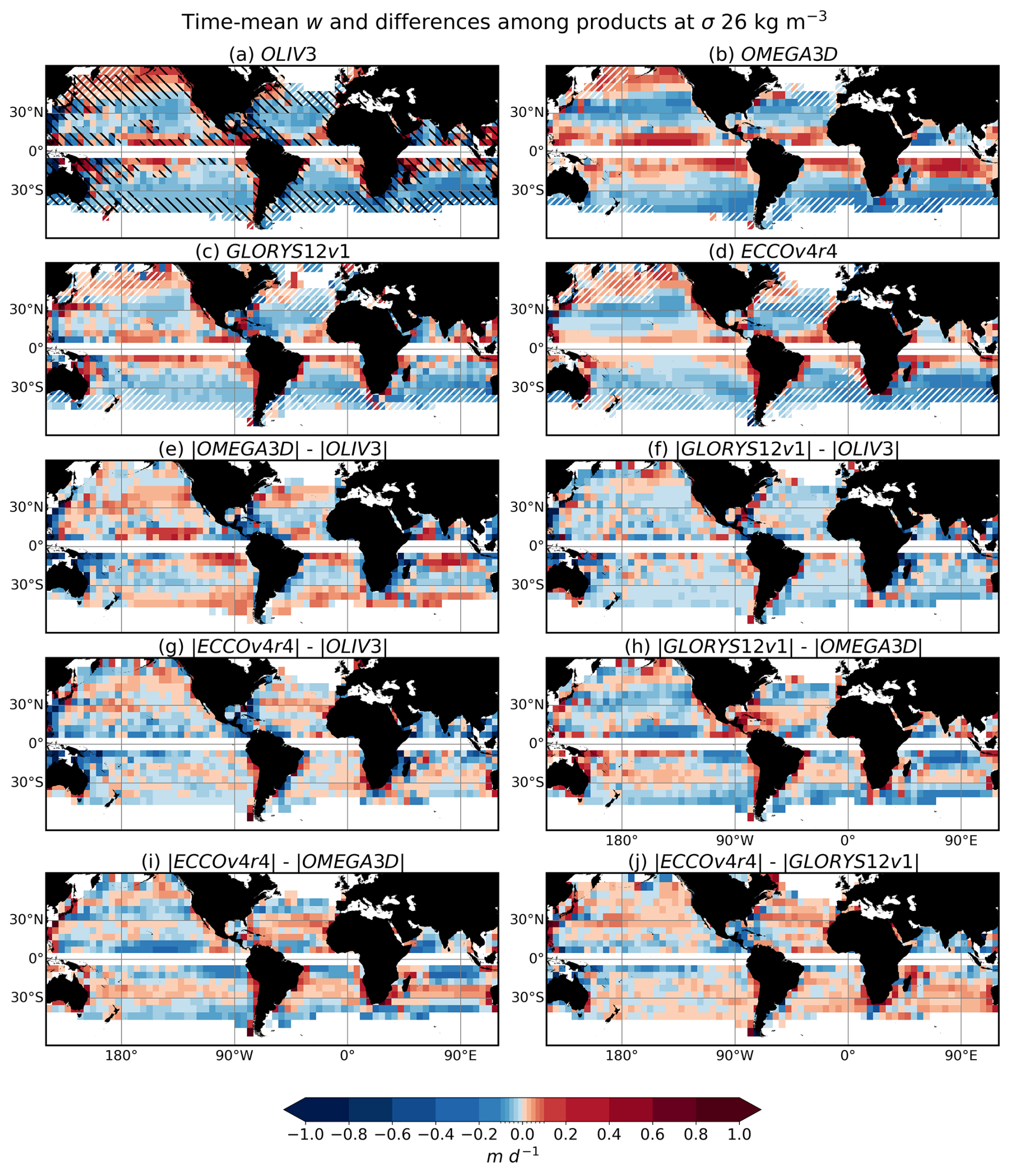
Figure 5 Time-mean vertical velocity fields at σ26 and 5°×5° spatial resolution from: (a) OLIV3, (b) OMEGA3D, (c) GLORYS12v1 reanalysis, and (d) ECCOv4r4 reanalysis. White hatching represents regions within the maximum mixed layer defined by the thermohaline field corresponding to each velocity. (e–j) Differences between absolute values of the various datasets. In panel (a), black hatching indicates the areas where the LVB is not satisfied in the OGCM (relative error >10 %).

In the tropics, OLIV3, ECCOv4r4 and GLORYS12v1 (Fig. 5a, c and d respectively) exhibit spatially variable upwelling across all the oceanic basins, including along the Pacific and Atlantic eastern boundaries (Elmoussaoui et al., 2005; Faye et al., 2015). OMEGA3D (Fig. 5b) captures a broader and smoother field with maximum upwelling at the centre of the basins. These OMEGA3D upwelling patterns were already reported in Buongiorno Nardelli (2020). Notably, the deep tropical band (5–10° N/S) show low agreement between reanalyses and OLIV3, matching the regions where the LVB errors in the OGCM exceed 10 % (black hatching in Fig. 5a). Some regions exhibit amplitude discrepancies among the three datasets (e.g. North Pacific tropical band), and some others even display opposite signs (e.g. Indian Ocean).

In subtropical latitudes, although OLIV3 and OMEGA3D reproduce the large-scale direction of the vertical flow, some regional differences emerge (Fig. 5e–i). For example, in the North Pacific, OLIV3 and GLORYS12v1 show a maximum downwelling centred near 30° N, 140° W, while OMEGA3D and ECCOv4r4 display strong downwelling across the entire 30° N band. In the North Atlantic, the downwelling maximum in OLIV3 and GLORYS12v1 is found in the southeastern part of the gyre. Nevertheless, OMEGA3D captures this maximum closer to the western boundary current extension, and ECCOv4r4 centres it at 30° N. In the South Atlantic and South Indian Oceans, all datasets reproduce maximum downwelling near the intersection of σ26 with the bottom of the mixed layer. In the South Pacific, only OMEGA3D presents a maximum near the intersection between the isopycnal level and the bottom of the mixed layer, GLORYS12v1 produces weaker amplitudes, and OLIV3 and ECCOv4r4 locate a maximum downwelling at around 30° S, 90° W.

Western boundary currents also reveal discrepancies. In the Gulf Stream and Kuroshio Current extensions, OLIV3 reproduces upwelling patterns consistent with Ekman pumping (Qiu and Huang, 1995), OMEGA3D and reanalyses, and captures strong downwelling at 30° N along the continental section of both currents. At this latitude, in the Gulf Stream case, OMEGA3D reveals some downwelling, while ECCOv4r4 displays positive vertical velocities, in agreement with other model results (GODAS and SODA, among others) shown by Liao et al. (2022). GLORYS12v1 reproduces upwelling and downwelling on both sides of the current. In the Kuroshio Current, ECCOv4r4, GLORYS12v1 and OMEGA3D feature mainly upward flow. The Brazil Current is associated with upwelling flow in all datasets, although OLIV3 tends to overestimate its amplitude.

One may argue that a likely source of discrepancies across the isopycnal level between OLIV3 and the reanalyses is that OLIV3 reconstructs only the geostrophic component of the vertical velocity, whereas the reanalyses estimate the total vertical velocity field. However, the comparison between OGCM's w_g and w_tot (Fig. 4a) illustrates better agreement in spatial patterns and intensity than when comparing OLIV3 with the reanalyses (Fig. 5a, c and d). For instance, in the subtropical gyres, where the relative differences between OGCM's w_g and w_tot are typically below 10 %, the differences between OLIV3 and any of the reanalyses often exceed this threshold (Fig. 5f and g). This suggests that much of the observed differences derive from the observation-based input fields (ARMOR3D meridional velocities and ERA5 wind stress) rather than the geostrophic component reconstructed, which mostly dominates the total flow in the subtropics and upper tropics. Particularly, western boundary current systems correspond to regions with large errors in the geostrophic LVB-derived vertical velocities (hatching in Fig. 5a). In these regions, additional terms of the vorticity equation, such as the bottom pressure torque, close the vorticity budget (e.g. Hughes and De Cuevas, 2001; Gula et al., 2015; Schoonover et al., 2016).

OLIV3 demonstrates a reasonable ability to qualitatively capture the time-mean vertical velocity structure of the major ocean gyres at σ26. Even in regions where the LVB assumption is no longer valid, such as the deep tropics, western boundary currents and the subpolar Pacific, OLIV3 estimates often remain within the uncertainty range defined by the intercomparison datasets.

3.3.2 Vertical structure of time-mean vertical flow

The presence of vertical shear in the vertical velocity field is fundamental for establishing the Sverdrup balance and defining the volumes of water influenced by these dynamics. In classical Sverdrup theory, vertical velocities in the deep ocean are assumed to be very weak, allowing the vertically integrated meridional transport to be related to the wind stress curl. Global estimates of the vertical velocity offer insights into the fundamental physics of the ocean interior circulation. When the LVB holds, geostrophic vertical velocities in the ocean interior can be interpreted as the residue of the evacuation by meridional transport of the vertical mass flow input from the layer above. If the geostrophic vertical velocity at a given depth is effectively negligible, the divergence of the horizontal flow fully compensates the wind-driven divergence above this level, implying that the Sverdrup balance adequately describes the ocean dynamics down to that depth. In this context, the vertical profile of the vertical velocity field adds information about the flow evacuation ratio under Sverdrup's framework. As demonstrated for the North Atlantic Ocean in CM24, this assumption holds reasonably well in subtropical basins but breaks down at high latitudes. This finding is consistent with recent studies that have directly evaluated Sverdrup balance (e.g. Thomas et al., 2014). Despite its relevance, studies focusing on the Sverdrup balance rarely address the vertical structure of the vertical velocity field.

To further evaluate the ability of OLIV3 to reproduce the vertical structure of the vertical flow, the vertical gradient of the absolute value of time-mean vertical velocity (Eq. 18) for multiple estimates of w is computed (Fig. 6). Most datasets (OLIV3, ECCOv4r4 and GLORYS12v1) feature a reduction in downwelling amplitude with depth across the subtropical gyres, consistent with a baroclinic structure (panels a, c, and d in Fig. 6). The largest negative gradients reach values above $-\mathrm{1.4}\times {\mathrm{10}}^{-\mathrm{4}}$ $\mathrm{m}{\mathrm{d}}^{-\mathrm{1}}{\mathrm{m}}^{-\mathrm{1}}$ in the global subtropical gyres. Compared with the rest of the estimates, OMEGA3D (Fig. 6b) displays a more barotropic profile (Fig. 6e, h, and i). OLIV3 (Fig. 6a) generally captures the reanalyses' downwelling weakening with depth in the subtropics (Fig. 6f and g). Nevertheless, it displays positive vertical gradients in the eastern tropical gyres, indicating increasing magnitude with depth, which contrasts with the other datasets. This difference may arise from a shallower thermocline at tropical latitudes compared to the subtropics (Salmon, 1982), which causes σ27 to lie below the bottom threshold of the thermocline. When the gradient is recalculated using σ26.5, as a lower limit, OLIV3 captures a negative gradient in both Pacific and Atlantic tropical gyres (Fig. A1). As for the North Atlantic application of LVB (CM24), tropical gyre's vertical velocities decrease rapidly in the thermocline, remaining an order of magnitude smaller than those at the top of the thermocline. This implies that the lower bounds of the gradient do not substantially bias the vertical structure in a model simulation, as seen in the small relative gradient error between OGCM w_tot and w_g in the Pacific and Atlantic tropical gyres (Fig. 4c). However, there are large uncertainties for observation-based datasets like OLIV3 compared to the reanalyses below the thermocline. OLIV3 shows growing vertical velocities with depth in regions where the time-mean vertical velocities at a given depth also differ, such as the western boundaries and the deep tropics. This suggests that when OLIV3 fails to capture the correct amplitude of the vertical flow, it also fails to reproduce the local vertical structure.

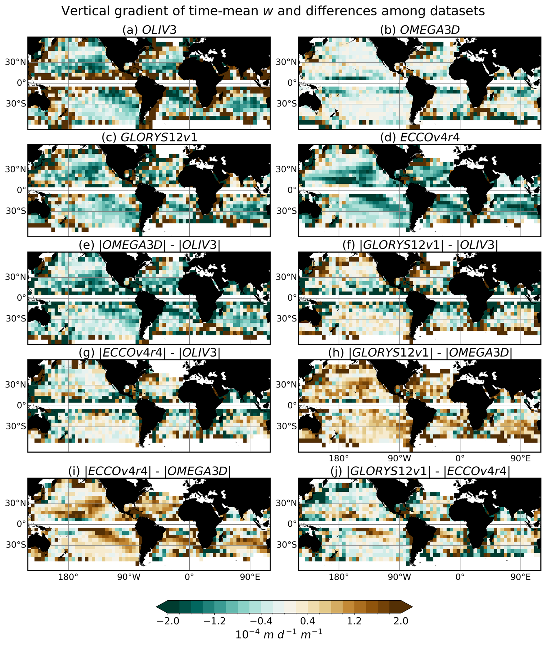
Figure 6 Vertical gradient of time-mean vertical velocity between the base of the maximum mixed layer depth and σ27 (Eq. 18) at 5°×5° spatial resolution, shown for: (a) OLIV3, (b) OMEGA3D, (c) GLORYS12v1, and (d) ECCOv4r4. Negative values indicate a decrease in vertical velocity magnitude with depth, while positive values depict increasing magnitude with depth. (e–j) Differences between absolute values in the vertical gradient of time-mean vertical velocity for the various datasets.

The comparison with existing estimates demonstrates that OLIV3 reproduces the structure in the subtropics and upper tropics (particularly above σ26.5), capturing both the amplitude and vertical structure of the vertical flow, indicating that the geostrophic component is the primary contributor to the observation-based vertical flow and that Ekman pumping vertical velocity is a suitable boundary condition, consistent with the results of the perfect model test.

3.3.3 Vertical velocity time variability

The perfect model test (Fig. 4) emphasises the high accuracy in terms of temporal variability of the total vertical velocity by the geostrophic component. To further assess this accuracy, we evaluate the annual variance and the correlation coefficient (R) across the various intercomparison datasets.

The key role of mesoscale activity (Wunsch, 2007) can be detected in the annual variance of vertical velocity at an isopycnal level within the tachocline (Fig. 7). In OLIV3, GLORYS12v1 and ECCOv4r4 (Fig. 7a, c, and d), the highest variance values are found along western boundary current regions and in the lower-tropical band, while the subtropical gyre interior below the mixed layer generally displays lower variance. This pattern is consistent with known regions of high mesoscale eddy activity at the ocean surface, such as the western boundary current systems and the deep tropics (e.g. Wunsch, 2007; Barceló-Llull et al., 2025), that is transported into the ocean interior. OMEGA3D (Fig. 6b) deviates from this behaviour, showing a poleward variance increase near the intersection of the isopycnal level with the ocean surface (Fig. 8a, d, and e). ECCOv4r4 (Fig. 7d) maintains a similar variance spatial distribution compared with OLIV3 and GLORYS12v1 but with a weaker variance gradient between the subtropical gyre centres and the western boundary current regions, due to lower maximum values (Fig. 8c and f). Variance values within the tropical Indian basin, as well as the western tropical Pacific and Atlantic basins, exhibit considerable uncertainty across datasets. Nevertheless, OLIV3 reconstructs a field with variance comparable to that in GLORYS12v1 (Fig. 8b), even in regions where LVB does not hold. This supports the ability of the geostrophic component to capture the temporal variability of vertical motion at first order, as evidenced by Fig. 4.

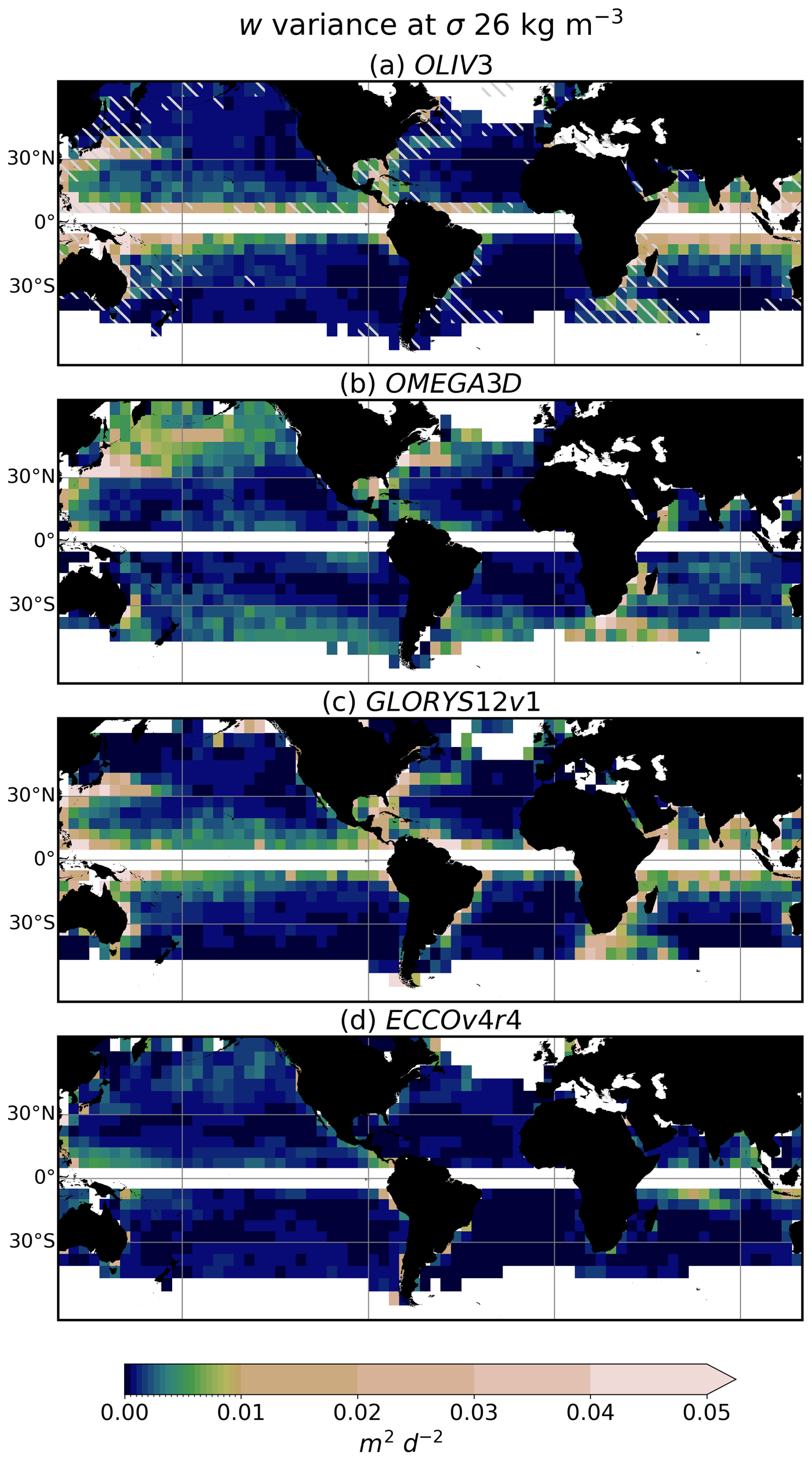
Figure 7 Annual variance of vertical velocity at σ26 and 5°×5° spatial resolution for: (a) OLIV3, (b) OMEGA3D, (c) GLORYS12v1, and (d) ECCOv4r4. In panel (a), gray hatching represents regions where the correlation coefficient between OGCM w_tot and OGCM w_g is smaller than 0.5 (Fig. 4b).

In addition to the variance, the ability of OLIV3 to represent interannual variability of w is evaluated through the correlation coefficient between dataset pairs at low resolution at the representative σ26 (Fig. 9) and as a function of latitude at three different sigma surfaces (Fig. 10). Across most dataset pairs, the highest correlation values are found in the centres of the subtropical gyres, while the lowest occur in the tropical band and western boundary currents. The comparison of the two reanalyses (Figs. 9a and 10) shows an overall relatively low correlation over large fractions of the global thermocline, with maxima within subtropical gyres and parts of the deep tropics, but with latitudinal median values remaining below 0.5 almost everywhere. The comparison of these two reference datasets provides reference values quantifying the uncertainties inherent to the estimation of the vertical velocity component of the flow.

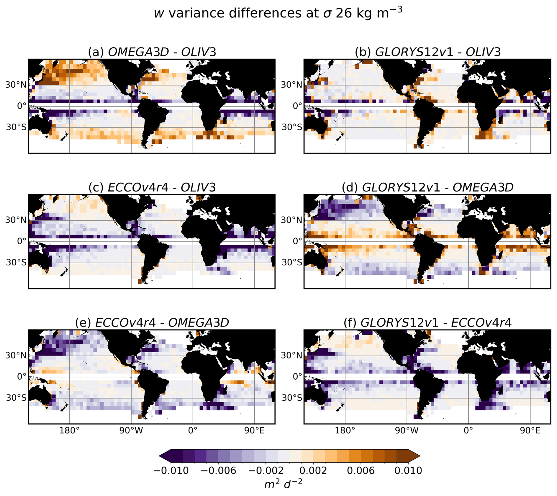
Figure 8 Difference between annual variances of vertical velocities at σ26 and 5°×5° spatial resolution for the various datasets in Fig. 7.

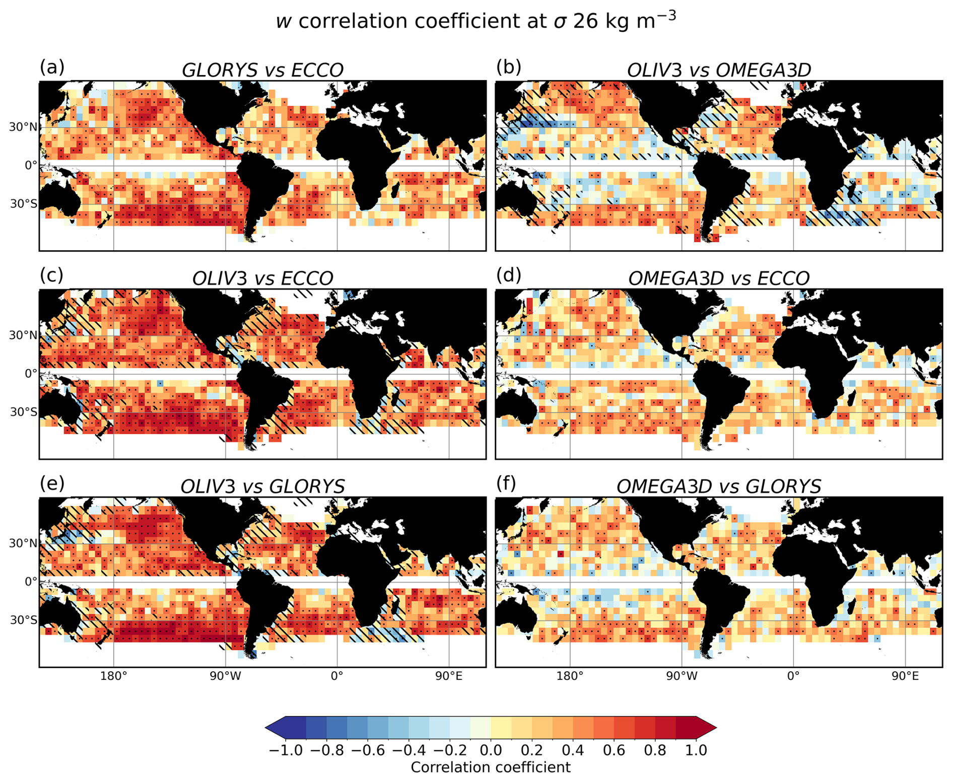
Figure 9 Correlation coefficient (R) between the vertical estimates from OLIV3, GLORYS12v1, ECCOv4r4, and OMEGA3D at σ26 and 5°×5° resolution. Dotted squares indicate correlations significant at the 95 % confidence level based on the Student t-test. Black hatching represents regions where correlation coefficient between OGCM w_tot and OGCM w_g is smaller than 0.5 (Fig. 4b).

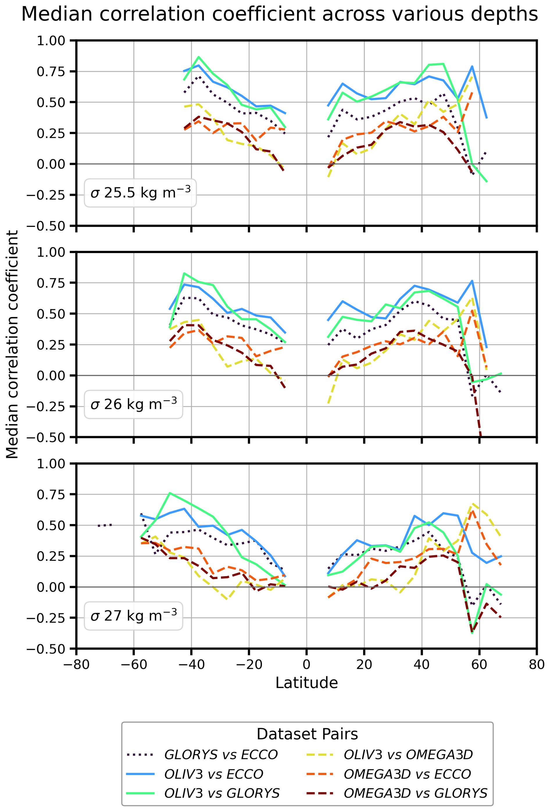
Figure 10 Median correlation coefficient (R) as a function of latitude for σ25.5, σ26 and σ27. The analysis includes only regions where the correlation between OGCM w_g and w_tot exceeds 0.5. Solid, dashed and dotted lines correspond to OLIV3, OMEGA3D intercomparisons, and renalyses intercomparison respectively.

OLIV3 exhibits significant high correlations (R>0.6) with the reanalyses across large portions of the global subtropics, with values exceeding 0.8 in the Pacific and Atlantic Oceans (Fig. 9c and e). In tropical regions where the perfect model test indicates weak correlation between w_g and w_tot (hatching in Fig. 9a), R typically falls below 0.4. Notably, reanalyses generally show a lower correlation with each other than with OLIV3 in most of the global subtropical band (Fig. 9a vs. 9c and e). The geostrophic component dominates the interannual variability of the vertical flow at these depths (Fig. 4). Therefore, the reduced inter-reanalysis correlation is likely evidence of the lack of synchronisation in the nonlinear components of vertical flow in assimilated products, while the geostrophic component variability, captured by OLIV3, remains highly correlated. The magnitude and structure of the variability reproduced by the OLIV3 fall within the range of variability spanned by very commonly used reanalysis-based estimates of w. Although OMEGA3D reaches significant correlation values (R up to 0.7) with the intercomparison reanalyses and OLIV3 in some areas within the open ocean, particularly within the Pacific and Atlantic subtropical gyres (Fig. 9b, d and f), its overall performance is poorer and more spatially limited compared to the results for OLIV3.

The general better performance of OLIV3 compared to OMEGA3D in capturing the temporal variability is further illustrated in Fig. 10, which displays the median correlation coefficient value as a function of latitude at three isopycnal levels. Latitudinal median correlation values between OLIV3 and ECCOv4r4 in the Northern Hemisphere subtropical band (20–40° N) are reduced from around 0.6 at σ25.5 to 0.4 at σ27. Although correlation coefficients between datasets tend to weaken with depth, OLIV3 (solid lines) consistently exhibits higher correlations with the model and reanalyses than OMEGA3D (dashed lines) throughout the entire thermocline except for high latitudes in the Northern Hemisphere.

3.4 Unveiling methodological differences among the existing estimates

Several fundamental methodological differences among OLIV3, OMEGA3D and the two reanalyses may account for the discrepancies observed in the climatological horizontal and baroclinic structure, as well as the temporal evolution of the vertical movements. These include the reconstruction methodology, the components of vertical velocity reconstructed, the atmospheric forcing, the three-dimensional horizontal velocity inputs, and the spatiotemporal resolution of the datasets.

Atmospheric forcing does not appear to be the primary source of discrepancies, as all datasets employ variants of ERA atmospheric reanalysis products to force the oceanic surface. Similarly, both OLIV3 and OMEGA3D are based on the ARMOR3D geostrophic velocity field, while reanalyses compute vertical velocities directly from the total assimilated horizontal velocity field. Despite their common input, OLIV3 and OMEGA3D exhibit large differences. In contrast, OLIV3 aligns more closely with the reanalyses despite their distinct origin in either observation-based or assimilated horizontal velocity fields. However, the ageostrophic component of the horizontal velocity field is negligible in most of the tropical and subtropical tachocline, as discussed in CM24. Again, while these differences may induce some discrepancies, they are not dominant.

Differences in native spatial and temporal resolution may play a significant role, even when data are averaged to a common resolution. Certain phenomena may persist across scales and not be entirely removed (Yeager, 2015). For example, GLORYS12v1 has a resolution of $\mathrm{1}/\mathrm{12}$°, capturing smaller mesoscale features compared to ECCOv4r4 at 1° resolution. Higher spatial resolutions allow GLORYS12v1 to preserve events at seasonal and sub-seasonal timescales, which could not be maintained in coarser native resolutions. Previous studies on reanalysis intercomparison (e.g. Balmaseda et al., 2015; Carton et al., 2019) have shown that such differences due to resolution (in particular in temperature and salinity) are more pronounced in the tropics. In particular, Carton et al. (2018) shows how the coarser resolution of ECCO leads to very distinct results from other eddy-permitting datasets. The spatial resolutions in the mentioned study range from 0.25 to 1°. Therefore, the uncertainty observed here between GLORYS12v1 and ECCOv4r4 probably reproduces and magnifies the uncertainty observed in the cited studies.

OLIV3 and reanalyses estimate w through vertical integration of horizontal velocity fields, because the governing equations only contain the vertical derivative of w. In contrast, OMEGA3D employs the omega equation, which, although it also requires vertical integration, explicitly includes second-order vertical derivatives and horizontal derivatives of w. Consequently, Dirichlet (vertical velocities are set to zero) and Neumann (partial derivatives of vertical velocity are set to zero) conditions are imposed as boundary conditions (Buongiorno Nardelli et al., 2018; Buongiorno Nardelli, 2020). The inclusion of the horizontal and second-order derivatives of w in the OMEGA3D framework may explain the discrepancies with the other datasets. However, a comprehensive examination of the sources of these differences would require a separate in-depth investigation, given the complex physics, constraints and assumptions underlying the omega equation.

3.5 Near surface interannual variability of vertical flow: improvement relative to Ekman pumping

Beyond the importance of providing an estimate of the vertical profile of thermocline vertical velocities, one might wonder how ocean interior w_g compares with Ekman pumping (w_Ek) from Eq. (9), the most commonly used observation-based reference product for vertical transfers between thermocline and nitracline, and the surface waters. Indeed, this wind-based computation is frequently employed to validate against observations, or calculate water mass fluxes (e.g. Marshall et al., 1993; Lazar et al., 2002), as well as transport of biogeochemical tracers (Oschlies, 2002) and marine ecosystem parameters, from fish (Parrish et al., 1981) up to whales (Croll et al., 2005). In these types of studies, Ekman pumping is generally considered as a vertical velocity proxy at a variety of levels depending on questions, time-scales and community habits. This level ranges from the bottom of the Ekman layer to that of the winter mixed layer (Williams et al., 2006), an isopycnal surface close to σ26 or a fixed depth of a few tens of meters up to 200 m (Palter et al., 2013). Here, the interannual synchrony of the Ekman pumping at the ocean surface and both the geostrophic and total vertical velocities is examined in isopycnal and depth coordinates (Fig. 11) to highlight the effect of the geostrophic current divergence on the variability of vertical velocities in the ocean interior. Specifically, Fig. 11a displays the correlation between w_Ek at ocean surface and w_tot on σ26, while Fig. 11b represents the correlation difference between w_g and w_tot shown Fig. 4b. Figure 11c and d illustrate, respectively, the correlation between w_g and w_tot at 100 m depth, and the correlation between w_Ek at the ocean surface and w_tot at 100 m depth. This comparison also illustrates the extent to which Ekman pumping can serve as a reliable proxy for describing the temporal variability of the total vertical flow within the ocean interior. Again, the computation is conducted with the reference OGCM simulation, considered to be a dynamically coherent estimate of the real ocean.

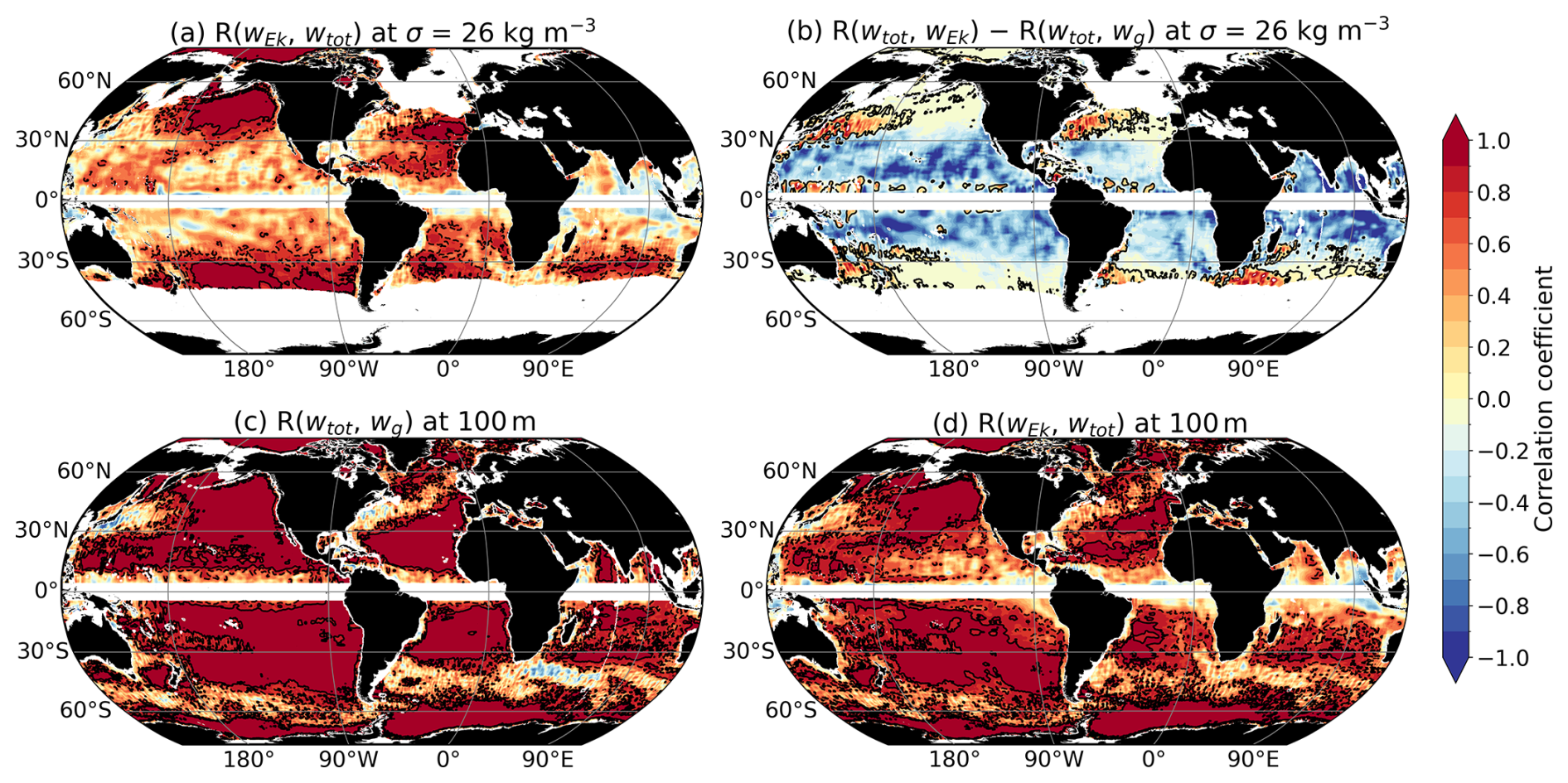
Figure 11 (a) Correlation coefficients between OGCM w at σ26 and Ekman pumping (1993–2015). (b) Differences between Figs. 4b and 11a. (c) Correlation coefficients between OGCM w and w_g at 100 m depth. (d) Correlation coefficients between OGCM w at 100 m depth and Ekman pumping. Same isolines as in Fig. 4b for panels (a), (c), and (d). For panel (c), the black contour lines represent the zero. The fields have been smoothed with a 5° running mean.

Ekman pumping estimates well (R>0.7) up to very well (R>0.9) the variability of total vertical velocities along σ26 over a relatively small proportion of the thermocline, limited to certain parts of the subtropical gyres and the tropical Atlantic Ocean (Fig. 11a). However, comparison with the correlation between w_tot and w_g (Fig. 4b), quantified in Fig. 11b, shows that w_g is accurate over much larger areas of the globe. In other words, w_Ek is only more accurate than w_g in regions where both estimates are poor (R<0.7), such as western boundary currents and intense open ocean currents, such as the NAD and ACC with a strong zonal component. Since w_g is derived from the geostrophic meridional velocity (v_g), this suggests that, in these regions, v_g reproduces an interannual variability not synchronised with w_tot, thereby further reducing the low correlation of w_Ek. Moreover, vertical movement in most eastern boundary upwelling systems, such as Benguela or Peru, shows weak correlations with Ekman pumping. This is consistent with the importance of remote forcing from trapped waves on the coast in these regions (Polo et al., 2008; Illig et al., 2014; Bachèlery et al., 2016). A marked decrease in the correlation coefficient is observed towards the western boundaries, where the isopycnal surfaces deepen, within the western boundary current systems, as well as in the deep tropics. When comparing this pattern to the correlation between w_g and w_tot shown in Fig. 4b, it is remarkable that the areas with high correlation are even more extensive in all basins.

We extended the comparison to other vertical levels, in particular to depths of 50 (not shown) and 100 m (Fig. 11c and d), and reached the same conclusion. Overall, these results show that the Ekman pumping alone is insufficient to account for interannual variability in vertical flow in most regions of the globe. However, the inclusion of geostrophic meridional transport divergence in Ekman pumping, i.e. w_g, brings about a significant improvement. This highlights the advancement of geostrophic vertical velocities as an estimator of total vertical flow variability.

4 Code and data availability

The OLIV3 dataset developed in this study is available at https://doi.org/10.5281/zenodo.16962780 (Cortés-Morales and Lazar, 2025). A low-resolution version, used in the intercomparison test of this study, is available upon request. Codes in MATLAB and Python to compute geostrophic velocities (OLIV3 and OGCM), apply the linear vorticity balance and calculate the intercomparison metrics are available at the following repository: https://doi.org/10.5281/zenodo.20398378 (Cortés-Morales et al., 2026).

5 Conclusions

This study introduces a novel observation-based global dataset of geostrophic vertical velocities (w) within the thermocline (Observation-based Linear Vorticity Vertical Velocities; OLIV3), which is presented and validated against other existing estimates. By applying the linear vorticity balance (LVB) to ARMOR3D meridional velocities and ERA5 Ekman pumping, OLIV3 provides a global physically consistent and observation-based framework to resolve large-scale vertical transport at a 0.25° horizontal resolution and annual frequency, covering the period 1993–2019. The dataset is available publicly at https://doi.org/10.5281/zenodo.16962780 (Cortés-Morales and Lazar, 2025).

The feasibility of the LVB framework for reconstructing vertical flow is demonstrated by the good agreement between the OGCM geostrophic vertical velocity estimates and the model's total velocity output. The spatial distribution and vertical shear of the temporal means of total velocity are well-reproduced by the geostrophic estimates, except in regions dominated by nonlinear dynamics such as the deep tropics and along western boundary currents. Furthermore, despite some mean biases across the globe, the model's geostrophic vertical velocity field effectively captures the interannual variability of vertical flow, with correlations exceeding 0.9 across most of the tropical, subtropical, and extratropical global oceans, excluding western boundary currents and also relatively intense zonal currents of the deep tropics, the NAD, and the ACC. This analysis confirms the dominance of geostrophic meridional transport in driving the interannual variability, while nonlinear components primarily influence the time-mean amplitude.

The comparison of OLIV3 against two reanalyses (ECCOv4r4 and GLORYS12v1) demonstrates that OLIV3 reproduces the large-scale horizontal patterns and baroclinic vertical structure of the climatological tachocline circulation over the 1993–2015 period. OLIV3 also captures the interannual variability in most of the open-ocean tropical and subtropical regions when compared to the reanalyses. The poorest performance of OLIV3 in the various metrics analysed is found across the same regions where LVB failed to reconstruct vertical flow in the OGCM perfect model test: western boundary currents, the zonal tropical currents, the NAD, and the ACC. Remarkably, OLIV3 often correlates as well or better with each reanalysis than the reanalyses do with each other, suggesting that the geostrophic signal variability is coherently captured, while nonlinear components suffer from a high degree of uncertainty in estimates of global ocean thermocline vertical velocities.

The intercomparison with OMEGA3D, the only other existing observation-based product, evidences the systematic improvement offered by OLIV3. OMEGA3D reproduces a relatively barotropic structure, which contrasts with the vertical shear observed in other products and the baroclinic ocean required to sustain the Sverdrup balance. Additionally, OMEGA3D exhibits an overall lower interannual synchrony with reanalyses. These discrepancies likely arise from the complexity of the omega equation compared to the LVB, including higher-order vertical and horizontal derivatives of w, that require boundary conditions extremely difficult to compute.

OLIV3 has been shown to be a useful tool for investigating interannual variability across the thermocline in polar, subtropical, and tropical gyres, with the exception of their western boundary currents, as well as most of the eastern boundary upwelling systems, offshore of the continental plateau. We strongly encourage its use in biogeochemical and biological studies focused on the vertical structure and exchange of ocean biogeochemical tracers, and on their impact on marine ecosystems, at interannual scales over large regions of the global ocean thermocline.

The wind-driven divergence at the surface and the vertical flow in the ocean interior are strongly correlated across large portions of the global tropical and subtropical gyres, as supported by the comparison between the OGCM estimation of the total vertical velocities in the ocean interior and Ekman pumping (w_Ek). However, geostrophic vertical velocities offer a systematically better or equal accuracy than Ekman pumping in capturing the interannual variability of the total vertical flow, except in regions of relatively intense zonal currents like the ACC, the tropical zonal currents and countercurrents, and the NAD, where both estimates exhibit limited confidence. These results emphasise the better performance of geostrophic vertical velocities as an estimator of the vertical flow variability in the ocean interior compared to the Ekman pumping alone. We propose to extend these findings to the real ocean, suggesting that OLIV3 provides a more accurate velocity field than Ekman pumping for estimating mass, and physical (temperature and salinity) and biogeochemical (nutrients, oxygen, CO₂) tracer fluxes between the surface and the pycnocline and nutricline layers. Observation-based knowledge of these flows is fundamental not only for a better understanding of the ocean's role in ongoing climate change but also for assessing the extent of oligotrophy, oxygen minimum zone, and acidification in the anthropogenic ocean.

In the future, OLIV3 could be improved to take into account seasonal and monthly scales and represent the specific processes of coastal areas while maintaining the simplicity of the depth-integrated formalism. Overcoming the current limitations in OLIV3 (spatiotemporal scales coarser than 5° and one year) would require incorporating total meridional velocities and additional terms from the vorticity equation, such as the horizontal advection of relative vorticity.

Appendix A: Supplementary figure

Figure A1 Vertical gradient of time-mean vertical velocity between the base of the maximum mixed layer depth and σ26.5 (Eq. 18) at 5°×5° spatial resolution, shown for: (a) OLIV3, (b) OMEGA3D, (c) GLORYS12v1, and (d) ECCOv4r4. Negative values indicate a decrease in vertical velocity magnitude with depth, while positive values depict increasing magnitude with depth.