Subsets of geostationary satellite data over international observing network sites for studying the diurnal dynamics of energy, carbon, and water cycles

The latest generation of geostationary satellites provide Earth observations similar to widely used polar-orbiting sensors but at intervals as frequently as every 5–10 min, making them ideal for studying the diurnal dynamics of land–atmosphere interactions. The NASA Earth Exchange (NEX) group created the GeoNEX datasets by collating data from several geostationary platforms, including GOES-16/17/18, Himawari-8/9, and GK-2A, and placing them on a common grid to facilitate use by the Earth science community. Here, we document the GeoNEX Coincident Ground Observations (GeCGO) dataset for terrestrial ecosystem studies and provide examples for its use. Currently, GeCGO provides GOES-16 Advanced Baseline Imager (ABI) data over a 10 km × 10 km area surrounding 1586 network sites across the Americas. GeCGO makes it easy to compare the time series of geostationary data with the diurnal ground observations, including carbon/water fluxes and aerosol optical depth, and is extensible to other regions. We also develop GeoNEXTools to facilitate analyses that require both GeoNEX data and other NASA satellite data. The objectives of this paper are to introduce GeCGO and GeoNEXTools and demonstrate their applications. First, we describe the details of GeCGO and GeoNEXTools. Second, we explain how GeCGO can be integrated with other satellite data. Finally, we showcase comparisons between GeCGO and observations from three ground-based networks. GeCGO is available at https://doi.org/10.25966/y5pe-xp41 (Hashimoto et al., 2025).

1 Introduction

Satellites monitor the Earth's surface using sensors with a variety of spatial-spectral-temporal characteristics. Sensors on geostationary satellites have unique characteristics, including high-frequency observations with a constant view zenith angle. Geostationary satellite data have been regarded as less effective for monitoring the Earth's environment due to their low spatial resolution and wide spectral bands. However, the latest generation of geostationary satellites have advanced imaging sensors, e.g., GOES-16/Advanced Baseline Imager (ABI) and Himawari-8/Himawari Advanced Imager (AHI), which can provide a spatial resolution (i.e., 1 km × 1 km) comparable with MODIS (Schmit et al., 2017). MODIS has been the most frequently used sensor for monitoring the global land surface for decades. The high-temporal-resolution data of the new geostationary satellites enable us to scrutinize sub-daily/sub-hourly processes on the Earth's surface, which polar-orbiting sensors with low temporal resolution like MODIS are unable to capture (Xiao et al., 2021; Yi et al., 2024). Therefore, the new generation of geostationary satellites have the potential to complement the polar-orbiting sensors for global- and continental-scale research.

Recent studies have demonstrated the effectiveness of using the new-generation geostationary satellite data for terrestrial ecosystem modeling. For example, Li et al. (2023b) used GOES ABI data to show that suppression of photosynthesis in the afternoon is caused by high vapor pressure deficits (VPDs) in the Western United States. Hashimoto et al. (2021) used the greater number of clear-sky observations from GOES ABI to analyze the leaf phenology over the Amazon and identify seasonal patterns in greenness. Others have shown that ABI data can be used to estimate sub-daily gross primary production (GPP) through a vegetation index (Khan et al., 2022), a machine learning technique (Stoy et al., 2024), or a light use efficiency model (Xiao et al., 2021). These efforts reveal the potential of using GEOS ABI for monitoring and modeling the dynamics of land surface vegetation. However, there remain difficulties for scientists in using geostationary satellite data due to their large volume, inconsistent file formats across sensors, and insufficient documentation or software to handle the data.

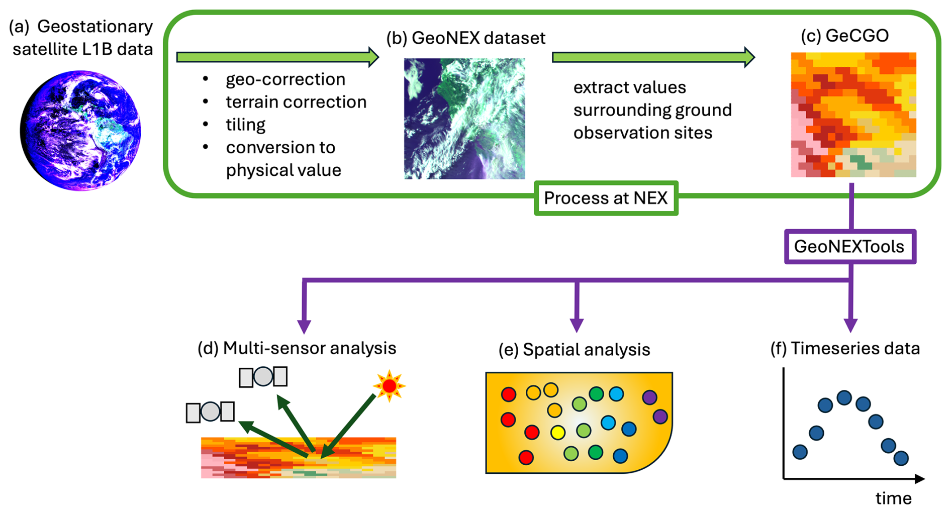
Figure 1 Flowchart showing how GeCGO is created. Geostationary satellite L1B data were used to produce the suite of GeoNEX datasets, then observations over the network site were extracted to create GeCGO (a–c). Users can download and analyze GeCGO data using GeoNEXTools for multi-sensor analysis (d), spatial analysis (e), and time series analysis (f).

Scientists faced similar challenges with MODIS data during the early days of the Earth Observing System (EOS) era. This led to the development of MODIS subset data (ORNL DAAC, 2017), which have since been extensively used by the land surface monitoring and modeling communities. The NASA Earth Exchange (NEX) recognized the importance of data compactness from the EOS experience and leveraged the GeoNEX project (Wang et al., 2020) to create the GeoNEX Coincident Ground Observations (GeCGO) dataset and facilitate the use of data from geostationary satellites. GeCGO is focused on widely monitored field and flux tower sites across the Americas and is accompanied by GeoNEXTools to help users retrieve GeCGO data, similar to the manner in which MODISTools supported the retrieval of MODIS subset data. The data processing flow is summarized in Fig. 1 and is implemented with Ziggy, an automated processing software for science data analysis pipelines (Tenenbaum and Wohler, 2024).

The objectives of this paper are to introduce GeCGO and GeoNEXTools and demonstrate their applications. First, we describe the details of GeCGO and GeoNEXTools. Second, we explain how GeCGO can be integrated with other satellite data. Finally, we showcase comparisons between GeCGO and observations from three ground-based networks.

2 Description of the GeoNEX data, GeCGO, and GeoNEXTools

2.1 GeoNEX dataset

The GeoNEX data are a collection of land surface images collected by new-generation geostationary weather satellites, including the Himawari-8/9 Advanced Himawari Imager (AHI), GOES-16/17/18 ABI, and Geo-KOMPSAT-2A (GK-2A) Advanced Meteorological Imager (AMI). Although intended for weather observations, the quality of the data from these satellites is now suitable for studying land surface dynamics. NEX has been producing geostationary data for land surface research communities from Level-1B full-disk scenes (Wang et al., 2020). The GeoNEX data are tiled into 6° by 6° with 0.005–0.02° spatial resolutions in geographic projection. Each sensor covers a square region approximately ± 60° from its nadir point to remove the edge pixels with a large viewing angle. Tiles including only oceans are not processed. Because the GeoNEX data were made from full-disk images, the temporal resolution is between 10 and 15 min.

We first georectified Level-1B data using information provided by institutions that operate the geostationary satellites. Although each sensor has its own state-of-the-art onboard georeferencing system, there are still residual pixel shifts in each image. For example, 1-pixel shifts for 500 m band data were observed almost every day in the AHI data, while ABI shifts were well under ± 0.5 pixel (Wang et al., 2020). The phase-only correction (POC) method was employed by matching Shuttle Radar Topography Mission (SRTM) digital elevation model (DEM)-based coastlines with the geostationary satellite images (Takenaka et al., 2020). We also corrected the relief displacement caused by the large viewing angle and high-elevation terrain, which is critical for comparing the satellite images with ground observation data.

The lowest level of the GeoNEX data is Level-1G, which contains top-of-the-atmosphere (TOA) reflectance and/or brightness temperature. The Level-2 data contain surface reflectance, which is retrieved by applying the Multi-Angle Implementation of Atmospheric Correction (MAIAC) (Lyapustin et al., 2011a). Other higher-level data are also available, i.e., land surface temperature (LST) data (Jia et al., 2022) and solar radiation data (Li et al., 2023a). Currently, the Level-2 LST data are available only for North America (i.e., Canada, US, and Mexico). The GeoNEX data are provided in the HDF-EOS2 format and available from the NASA Advanced Supercomputing Data Portal (https://data.nas.nasa.gov/geonex, last access: 29 September 2025).

NOAA also provides the ABI land Level-2 products, such as TOA reflectance, TOA brightness temperature, bidirectional reflectance distribution function (BRDF), and fire classification (Losos et al., 2024). The differences between the GeoNEX data and NOAA Level-2 products are that the GeoNEX data are (1) geo-corrected for each image, (2) reprojected to the geographic projection, (3) tiled for each area covering 6° by 6°, and (4) compiled such that they include international geostationary satellite data (see Wang et al., 2020, for more details).

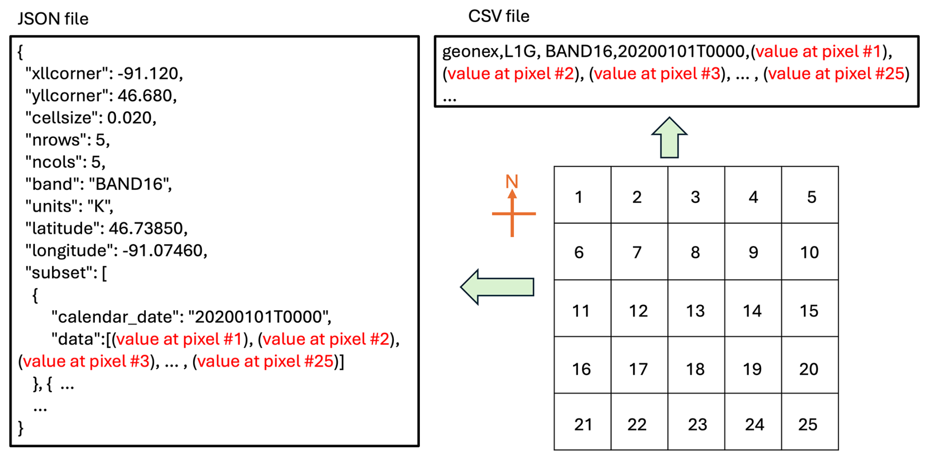
Figure 2 Example of JSON file and CSV file. The number in the 5 × 5 grid indicates the pixel position in the grid to clarify the order in the JSON and CSV files.

2.2 GeCGO

To make it convenient for users to get time series of GeoNEX data where ground-based observations are collected, we created GeCGO by extracting observations from the GeoNEX data over 1586 field or flux tower sites in various observation networks. To further facilitate its use, GeCGO is provided in the same file format as the Oak Ridge National Laboratory (ORNL) Terrestrial Ecology Subsetting & Visualization Services (TESViS) fixed sites subset data (https://modis.ornl.gov/sites/, last access: 29 September 2025) (ORNL DAAC, 2017), formerly known as MODIS/VIIRS Subset Tools, which will be familiar to most scientists. Specifically, GeCGO data are available in the comma-separated value (CSV) and JavaScript Object Notation (JSON) formats for each year (see the example of Fig. 2 and Table 1 for metadata descriptions). The data values were organized as 17 × 17, 9 × 9, and 5 × 5 grids for 0.005, 0.01, and 0.02° resolution, respectively. For instance, the TOA band 1 reflectance data has a 0.01° spatial resolution at nadir, and thus its GeCGO data consist of 9 pixel × 9 pixel value data. The data values represent sequences of pixels from the northwest corner to the southeast corner in row-major order (Fig. 2). The data are organized into directories named after the site IDs used in the TESViS Subset. Currently, we provide the Level-1G and Level-2 data within the GeCGO products, available at the NASA GeoNEX data portal (https://data.nas.nasa.gov/gecgo/data.php, last access: 29 September 2025). The available GeoNEX data are summarized in Table 2.

Table 1 The metadata in the GeCGO JSON file.

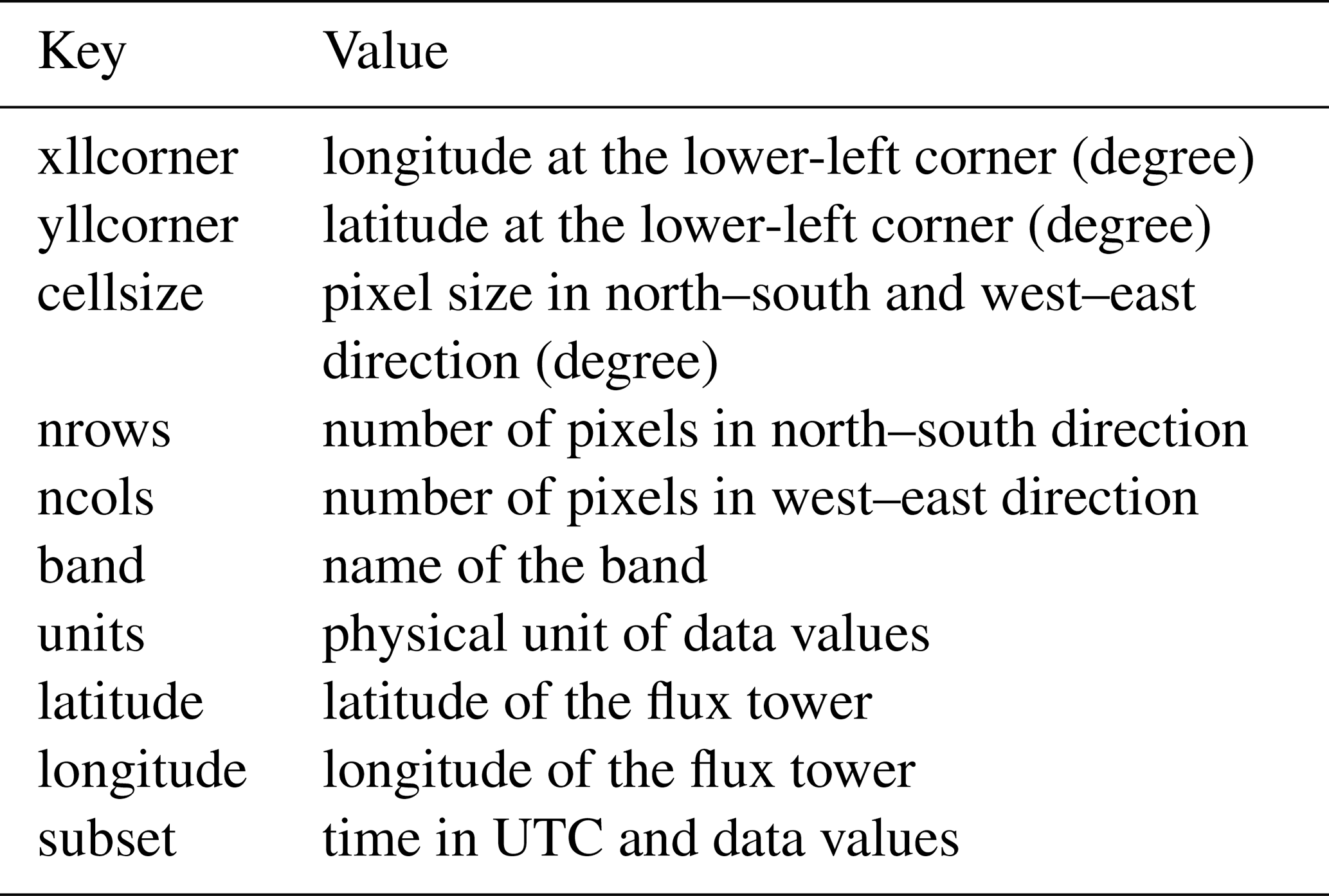
Table 2 The product summary of GeCGO. Each product has several bands with different spatial resolutions and grid sizes.

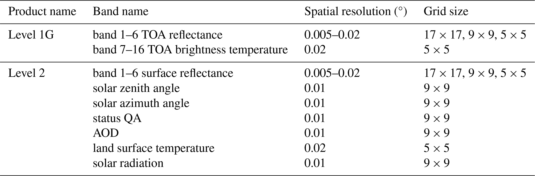
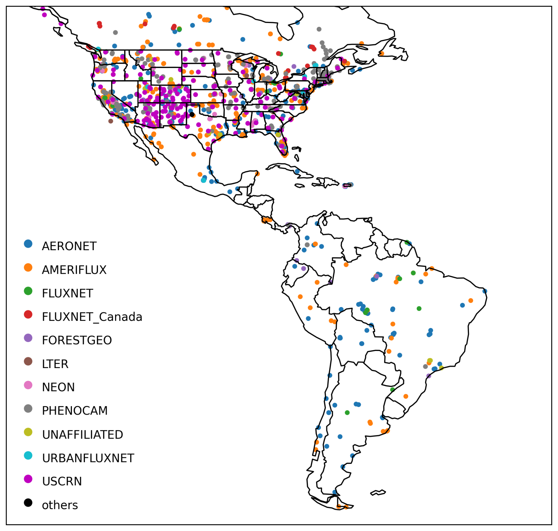
Figure 3 Spatial map of locations in the GOES16 coverage for each network used in GeCGO. The colors of dots represent various network names. Networks with less than 10 sites were categorized as “others”.

Table 3 Network names and number of sites of each network in the current GeCGO. Networks that had less than 10 sites were categorized as “others”. Each site was assigned only a single network based on TESViS data, though there were many sites that were involved in multiple networks.

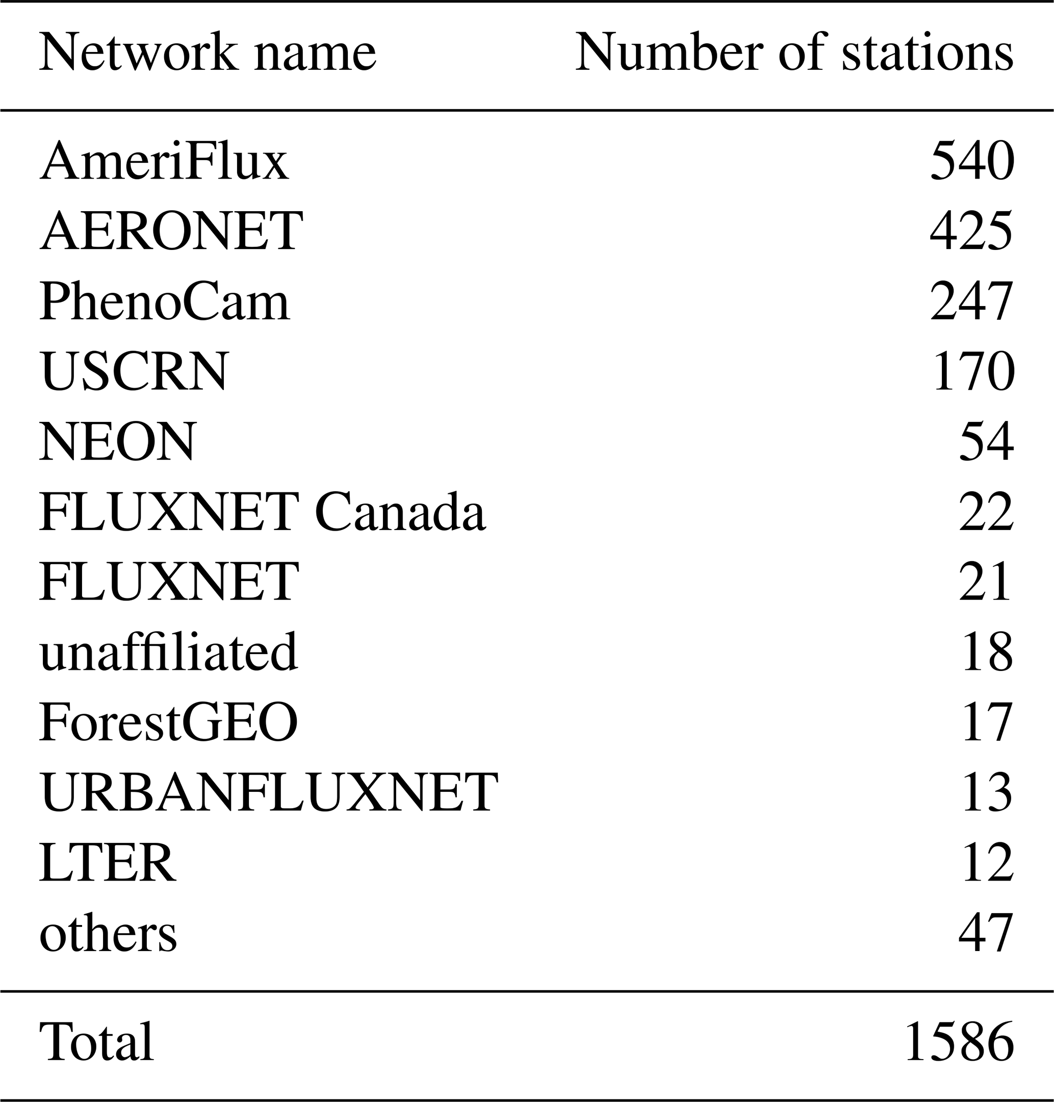
GeCGO has the same ground network information as the TESViS Subset and currently includes 1586 sites across 14 ground networks in the Americas. The GeCGO sites were entirely distributed over the continents in GOES-16 coverage (Fig. 3). Approximately 76 % of the sites are in the AmeriFlux (Chu et al., 2023; Novick et al., 2018), AERONET (Aerosol Robotic Network) (Holben et al., 1998), and PhenoCam (Richardson et al., 2018a) networks (Table 3). We excluded the island AERONET sites where the island area is less than 1000 km².

There is another existing subset of geostationary satellite data products over AmeriFlux sites (Losos et al., 2024). This subset of data provides half-hourly ABI fixed grid products for the AmeriFlux sites, including TOA reflectance, surface reflectance, cloud mask, aerosol, and solar radiation. Those data were single-pixel time-series-derived mainly from NOAA high-level products with the terrain correction. The ABI fixed grid products have different algorithms and procedures from GeCGO. For instance, GeoNEX and NOAA use different atmospheric correction (MAIAC (Wang et al., 2022) for GeoNEX and 6S (He et al., 2019) for NOAA) and geolocation correction (further orthorectification and geolocation correction in GeoNEX; Wang et al., 2020) algorithms. The different processing algorithms and procedures also make the spatial resolution and time step different. There are many ongoing international efforts to develop geostationary satellite products for various applications. We believe that the subset datasets, including GeCGO and the ABI fixed grid products, available through global ground networks provide ready-to-use hypertemporal Earth observations and inter-comparison data that can advance modeling and address important scientific questions.

2.3 GeoNEXTools

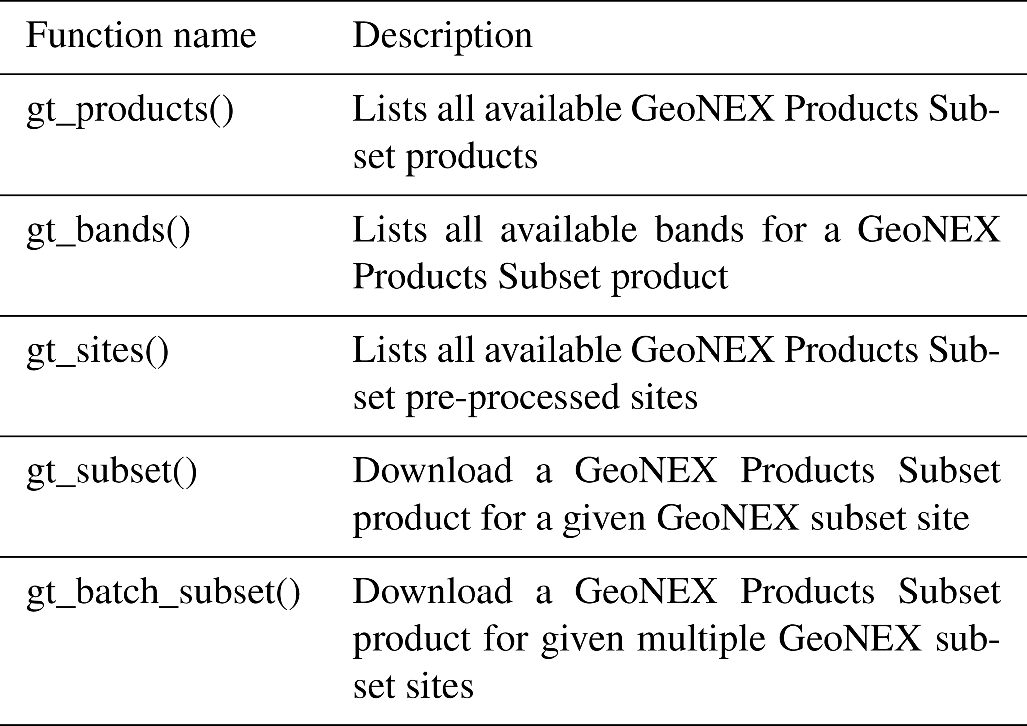
We developed GeoNEX Subset Tools, or GeoNEXTools (https://github.com/nasa/GeoNEXTools, last access: 29 September 2025), to facilitate downloading and manipulating GeoNEX data for specific ground observation sites and time ranges. Although the GeCGO data volume is smaller than the original GeoNEX full-disk and tiled data, handling GeCGO data remains challenging due to the length of the high-frequency time series. The MODIS science community solved a similar issue by developing MODISTools (Tuck et al., 2014), which is an open-source R package that helps users download and read the MODIS Subset data (https://github.com/ropensci/MODISTools, Hufkens, 2025). The MODISTools package has become one of the most widely used tools for handling TESViS Subset data. Because many scientists are accustomed to using MODISTools, we developed GeoNEXTools to provide functionality similar to that of MODISTools. The function names in GeoNEXTools are the same as those in MODISTools except for the prefix (e.g., mt_< function name> for MODISTools and gt_< function name> for GeoNEXTools). A full list of the function names and descriptions is provided in Table A1.

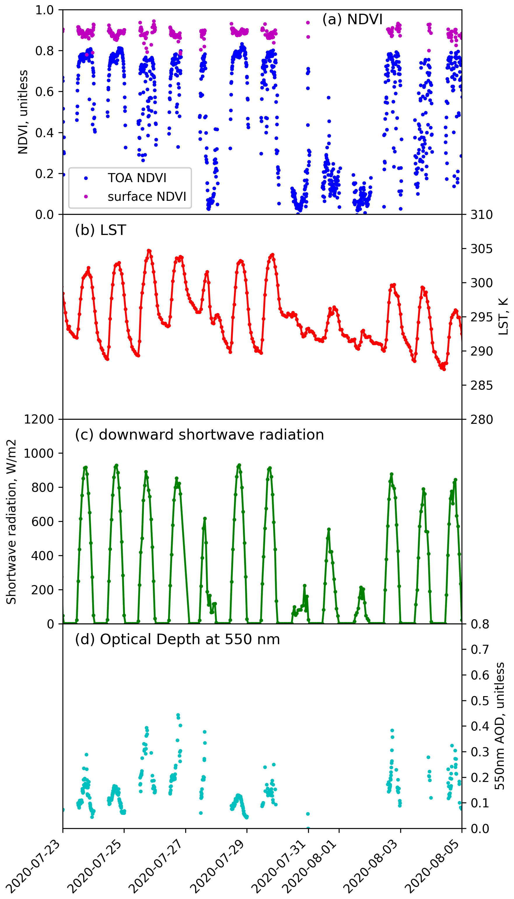
Figure 4 Time series from GeCGO at Harvard Forest EMS Tower (US-Ha1) from 23 July 2020 to 5 August 2020. (a) NDVI calculated from band 2 and band 3 at a 10 min interval. Blue and purple dots were top-of-the-atmosphere (TOA) (Level-1G dataset) and surface (Level-2 dataset) NDVI, respectively. (b) Land surface temperature (LST) at hourly intervals. (c) Downward shortwave radiation at hourly intervals. (d) Aerosol optical depth at 550 nm at a 10 min interval.

Figure 4 illustrates how GeCGO and GeoNEXTools can be used to analyze the diurnal variation in biophysical and meteorological variables. The figure includes data from the Harvard Forest EMS Tower (US-Ha1) from 23 July to 5 August, 2020, and clearly illustrates the diurnal variability in NDVI, LST, downward shortwave radiation, and aerosol optical depth (AOD). Preliminary examination of the data reveals several other insights. A cloudy day, i.e., 30 July to 1 August, is clearly evident in the diurnal variation in LST, which is smaller than on the other days. Figure 4a shows inverse patterns in diurnal surface and TOA NDVI on clear days (23 to 26 July), which indicates the importance of an atmospheric correction study in diurnal cycle studies. The clear-day NDVI calculated using TOA data shows peak values at noon, while the diurnal variation of the surface NDVI exhibits a U-shaped curve. Even though each of the GeoNEX products contains a large volume of data, GeoNEXTools significantly simplified the process of retrieving and examining single-point time series.

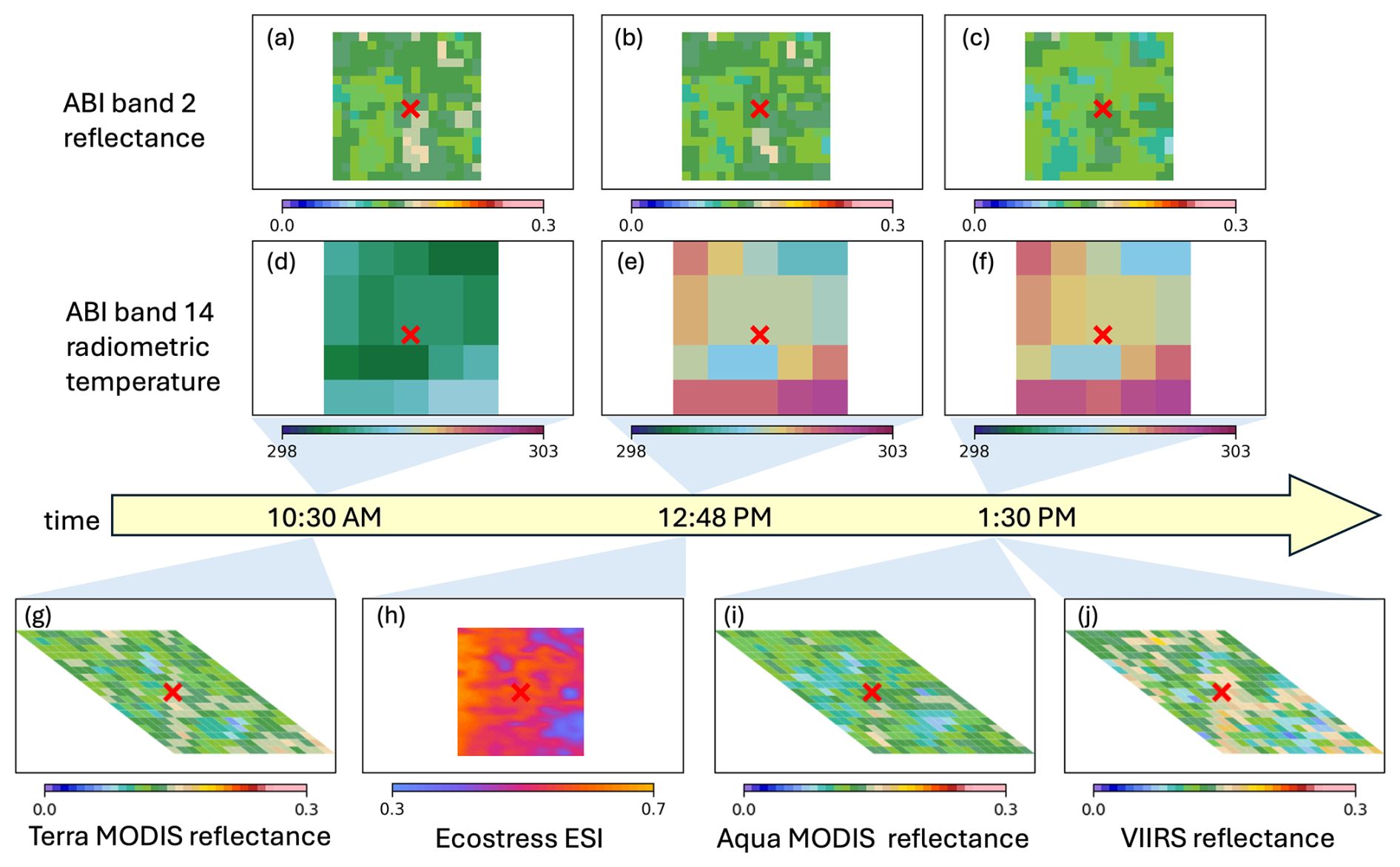
Figure 5 Example of instantaneous satellite observations in a single day (7 June 2020) at the Bondville, Illinois, flux tower site. The yellow arrow represents the time of the day in local time (Central Daylight Time, UTC − 5). The two-dimensional images were obtained from GeCGO or the TESViS Subset. The ABI band 2 reflectance (0.59–0.69 µm) subset data are shown in the upper row of panels (a–c). The ABI band 14 radiometric temperature subset data are shown in the middle row of panels (d–f). The lower panels show the low Earth orbit satellite data: Terra MODIS reflectance (MOD09A1) band 2 (0.84–0.88 µm) (g), ECOSTRESS Evaporative Stress Index (ESI) (h), Aqua MODIS reflectance (MYD09A1) band 2 (0.84–0.88 µm) (i), and VIIRS reflectance (VNP09A1) band I1 (0.60–0.68 µm) (j). The outside boundaries of the black line box for each satellite image have the same spatial extent, i.e., 40.06–39.96° N, 88.3811–88.1970° W. The red cross shows the location of the Bondville flux tower (40.0062° N, 88.2904° W). The light-blue triangles indicate the approximate observation time of each satellite image.

3 Use cases

3.1 Pairing GeCGO data with TESViS Subset data for scientific insight

One of the key advantages of GeCGO is its ability to be combined with data from polar-orbiting satellites. Creating GeCGO in the same format as the TESViS Subset makes it easy to integrate and analyze the two datasets together. Figure 5 illustrates the approach, combining multiple satellite data from the TESViS Subset with GeCGO. Satellite observations are usually made at different times of the day. For example, Terra and Aqua MODIS observe their target around 10:30 AM and 1:30 PM local time, respectively. The observation time of sensors on board ISS (e.g., ECOsystem Spaceborne Thermal Radiometer Experiment on Space Station, or ECOSTRESS) varies due to changing altitude and orbital inclination of the station. As a result, the phenomena in ecosystem processes observed by different satellite sensors could be specific to the observation time. Thus, using single satellite data may lead to biased results. Using multiple satellites can overcome the observation-time issue, and the geostationary satellite data can serve as a bridge between the instantaneous observations from multiple satellites. For example, the drought impact on vegetation quantified by ECOSTRESS's instantaneous evaporative stress index (ESI) can be temporally extended to an entire day using radiometric temperatures from geostationary satellite data. In addition, the spatial pattern of drought impacts can be scrutinized using reflectance and radiometric temperature from MODIS or VIIRS finer-spatial-resolution data (Xiao et al., 2021). Such analyses can be easily implemented using the GeCGO and TESViS Subset data (Fig. 5). Beyond the analysis of diurnal changes, GeCGO can be useful for BRDF modeling, which requires observations from multiple sun-target-satellite geometries (e.g., Adachi et al., 2019). Combining GeCGO with the TESViS Subset can help users find the scenes that meet their research needs.

Spatial resolution and projection differences between a geostationary satellite and other low Earth orbit satellites (e.g., MODIS, VIIRS) are challenging issues for users interested in using them together for various scientific applications. We thus chose to convert the geostationary satellite view projection to geographic projection for its easy useability. The original Level-1b data of GOES ABI is skewed at the edge of the coverage, where the viewing angle is large. Meanwhile, the TESViS Subset data has different projections for each product. For example, MODIS data in the TESViS Subset were reprojected from swath images to sinusoidal projection. As a result, the MODIS subset data show the skew cutout as shown in Fig. 5g and i. Therefore, matching all the pixels between the subset data is not straightforward. Using only the center pixels where the ground observation sites exist is the easiest way to avoid such complex projection conversion processes.

3.2 Examples of using GeCGO with ground observation network data

3.2.1 AmeriFlux: can NDVI or NIRv represent annual GPP?

AmeriFlux is a network of sites that use the eddy covariance technique to measure ecosystem CO₂, water, and energy fluxes across North, Central, and South America (Chu et al., 2023). Due to its wide distribution across diverse ecosystems and climate gradients, AmeriFlux data have been used for validating satellite products (Baldocchi et al., 2001) and for upscaling site-specific observations from AmeriFlux sites to regional and global scale using remote sensing data (Running et al., 2004). However, because each MODIS on TERRA or AQUA provides only one observation at a specific time of the day in the daytime, converting MODIS observations to representative daily values requires various assumptions or models to align with the daily average of the half-hourly observations provided by AmeriFlux products. In contrast, the geostationary satellite data can be directly compared with the half-hourly AmeriFlux data. Several data-driven models using geostationary satellite data have been proposed to estimate carbon and water fluxes (Khan et al., 2022; Li et al., 2023b; Stoy et al., 2024; Xiao et al., 2021) and vegetation indices for tracking the diurnal cycle of GPP (Jeong et al., 2023). Given the dynamic nature of fluxes and the environmental factors that influence them throughout the day, combining hypertemporal geostationary satellite data with AmeriFlux data provides a more accurate representation of diurnal variations in fluxes compared to using polar-orbiting satellite data. GeCGO further enables users to work with specific datasets without needing to download the entire GeoNEX data, making it especially valuable for model development.

As an example of using AmeriFlux data, we compared annual GPP with mean NDVI and NIRv (Badgley et al., 2019) to analyze the spatial representation of vegetation indices from ABI data in 2018 (Fig. 6). The annual GPP was obtained from the AmeriFlux FLUXNET data product (Pastorello et al., 2020) for each site. The mean annual NDVI and NIRv were derived from daily values of NDVI and NIRv, and the daily NDVI and NIRv were calculated from the median of the 90th percentile data for each day. Unlike TOA products (i.e., L1G), L2 data contain significant gaps due to the cloud mask derived from the MAIAC algorithm. Therefore, we excluded the AmeriFlux sites with fewer than 100 d of available daily data.

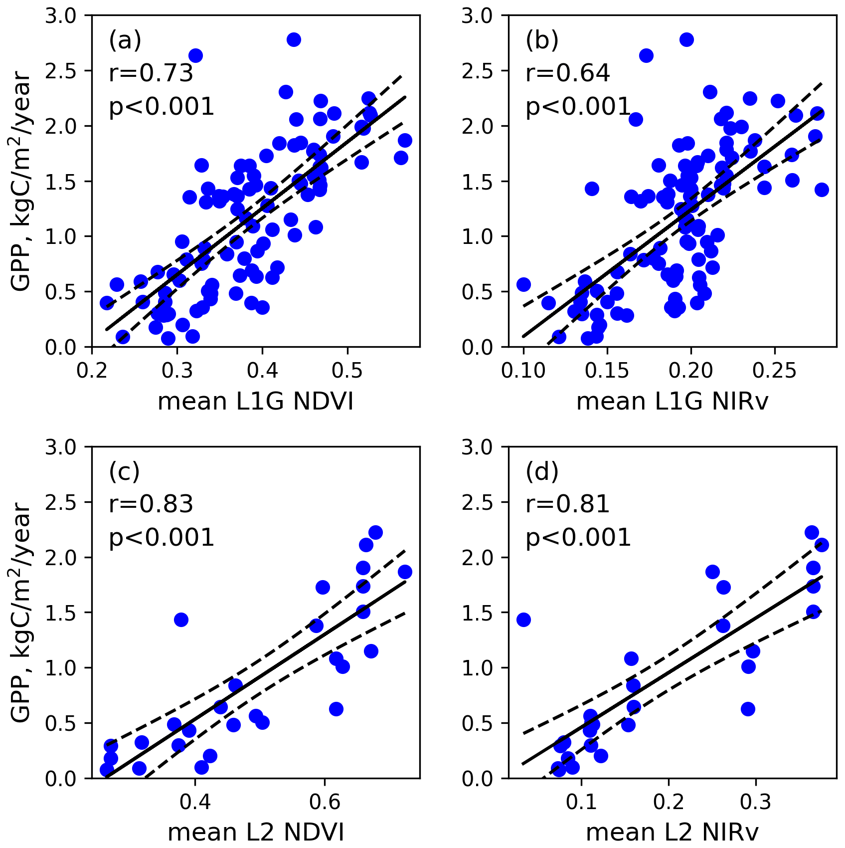
Figure 6 Scatter plot (blue dots) of annual GPP ($\mathrm{kg}\mathrm{C}{\mathrm{m}}^{-\mathrm{2}}{\mathrm{yr}}^{-\mathrm{1}}$) at AmeriFlux sites against mean L1G NDVI (a), mean L1G NIRv (b), mean L2 NDVI (c), and mean L2 NIRv (d). The solid line is a linear regression line. The dashed lines represent the 95 % confidence intervals of the regression.

We found significant relationships across all comparisons between mean annual GPP and vegetation indices (VIs). Even TOA VIs, which did not undergo cloud screening, had high correlations (r = 0.73 for NDVI and r = 0.64 for NIRv) with annual GPP (Fig. 6a and b). Moreover, surface VIs showed strong correlation with GPP compared to TOA VIs (r = 0.83 for NDVI and r = 0.81 for NIRv) (Fig. 6c and d), suggesting that surface reflectance VIs better represented spatial patterns of annual GPP despite the limited data availability. For both L1G and L2, NDVI showed a slightly stronger correlation with annual GPP than NIRv.

However, these results do not imply that NDVI is inherently better than NIRv for representing the spatial variability of annual GPP. The resolutions of the GeoNEX datasets are greater than 0.005° (approximately 500 m at the nadir). While a spatial resolution of 500 m may be comparable to the footprint of many flux sites, this resolution applies only to a red visible band (0.64 µm) of ABI at the nadir. As a result, high spatial heterogeneity within the pixels can lead to a scale mismatch between the flux data and the GeoNEX data footprints, although this footprint scale mismatch issue is not limited only to GeoNEX datasets. Chu et al. (2021) provide representativeness information of the tower footprint for all AmeriFlux sites. We encourage users to consult with the footprint information to select appropriate sites for directly analyzing the relationship between flux data and GeCGO. Additionally, in this example, we did not account for other factors such as BRDF dependency on sun-target-satellite geometry (Morton et al., 2014). Further analysis, considering these factors, would provide a more appropriate conclusion regarding the spatial representation of vegetation indices.

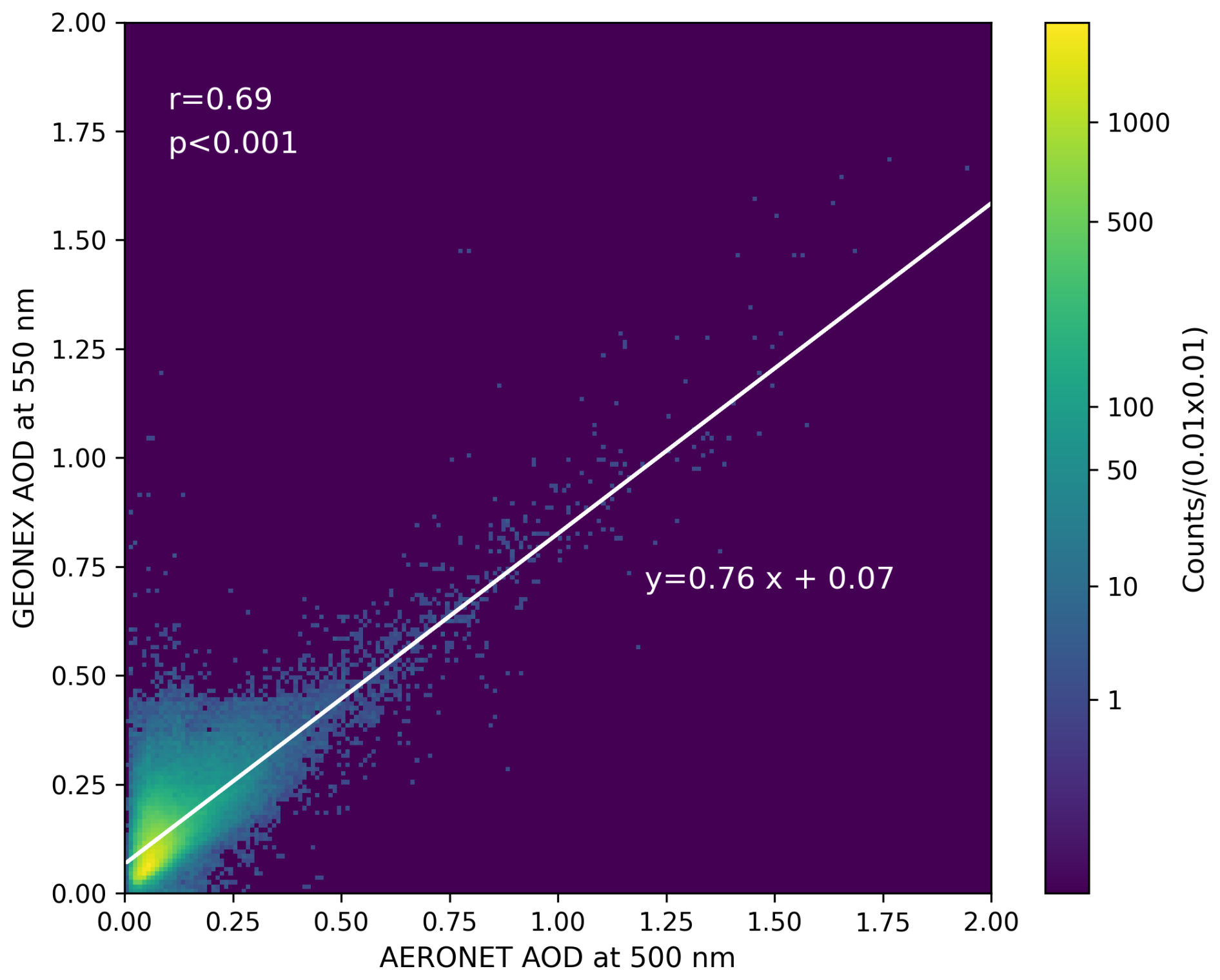
Figure 7 Density plot of the GeCGO AOD at 550 nm against the AERONET AOD at 500 nm. The white line represents the linear regression line. The plot includes only 2019 data over the GOES 16 coverage area.

To validate and calibrate VIs derived from GeCGO, high-frequency vegetation indices estimated at the ground level can be valuable. For example, some scientific instrument manufactures produce sensors capable of measuring NDVI at sub-hourly intervals (e.g., Apogee Instruments, Holland Scientific). While these sensors can be installed on flux towers and are used at some sites, they are not standard components of flux towers. More notably, a group of flux and remote sensing scientists recently developed a method to derive sub-hourly NDVI and NIRv using quantum sensors and pyranometers, which are commonly installed on flux towers (Mallick et al., 2024). This approach can be used to validate and calibrate VIs derived from geostationary satellites, addressing footprint mismatches, improving accuracy, and reducing uncertainties.

3.2.2 AERONET: validation of the Level-2 AOD products using AERONET AOD

AERONET is a global aerosol monitoring network that monitors the aerosol optical depth using sun photometers. The time interval of observation is less than an hour. The aerosol optical depth (AOD) has large diurnal variability. Therefore, the sub-hourly observations of GOES data are suitable for large-scale AOD estimation compared to once-a-day observation of polar-orbiting satellites (Sorek-Hamer et al., 2020). AOD in the GeoNEX Level-2 data is a product of estimating surface reflectance using MAIAC (Lyapustin et al., 2011b).

To assess the accuracy of GeoNEX Level-2 AOD estimates, we compared the AERONET version 3 data (Sinyuk et al., 2020) to the GeCGO AOD data. AERONET provides the AOD data estimated from sun photometer radiance measured approximately every 3 min. We plotted the GeCGO AOD data against AERONET version 3 data for matching times within 2 min in 2019 (Fig. 7). In this example, the GeCGO AOD overestimated the AERONET AOD, especially for low AOD less than 0.3. GeCGO will facilitate the development of an AOD estimation algorithm and will contribute to improving high-temporal AOD estimation algorithms for the geostationary satellite mission focusing on air quality monitoring (i.e., Tropospheric Emissions: Monitoring of Pollution (TEMPO), Global Environmental Monitoring System (GEMS), and Sentinel-4).

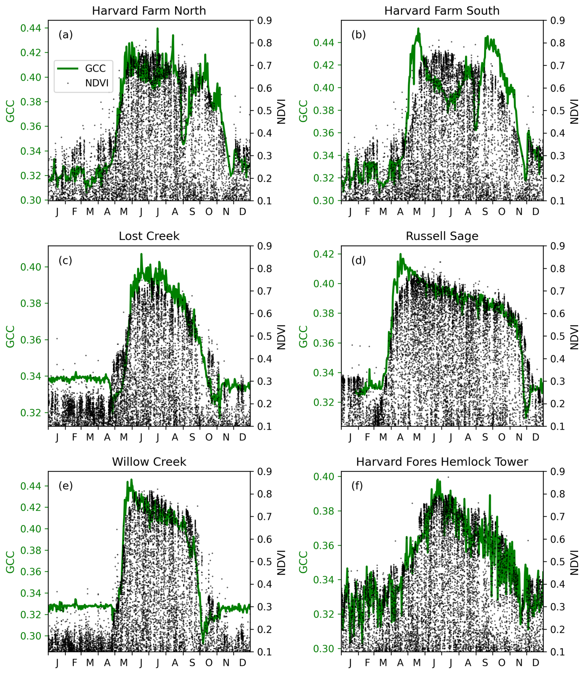
Figure 8 Examples of time series of L1G 1 km NDVI (black dot) and the Green Chromatic Coordinate (GCC) (green line) at six PhenoCam sites in 2019. (a) Harvard Farm, Petersham, MA (ID: harvardfarmnorth, 42.5205° N, 72.1822° W, grassland). (b) Harvard Farm South, Petersham, MA (ID: harvardfarmsouth, 42.5225° N, 72.1823° W, grassland). (c) Lost Creek, WI (ID: lostcreek, 46.0827° N, 89.9792° W, deciduous shrub wetland). (d) Russell Sage State Wildlife Management Area, LA (ID: russellsage, 32.4570° N, 91.9743° W, deciduous broadleaf). (e) Willow Creek, Chequamegon–Nicolet National Forest, WI (ID: willowcreek, 45.8060° N, 90.0791° W, deciduous broadleaf). (f) Hemlock Tower, Harvard Forest, Petersham, MA (ID: harvardhemlock2, 42.5394° N, 72.1780° W, evergreen needleleaf).

3.2.3 PhenoCam: time-series comparison between L1-G NDVI and PhenoCam greenness

PhenoCam is a phenology ground observation network using time-lapse cameras. Each site provides time series of digital camera images, with the objective of capturing the seasonal cycle of vegetation phenology (Richardson et al., 2018b). PhenoCam provides daily statistics of the image values, including the daily Green Chromatic Coordinate (GCC). The GCC was calculated by dividing the Green Digital Number (DN) by the sum of the Red, Green, and Blue DNs. The DNs of the PhenoCam were extracted from regions of interest (ROIs), which focus on dominant vegetation types in the images. The GCC time series aligned well with the polar-orbiting satellite NDVI (Richardson et al., 2018a). Miura et al. (2019) reported that the geostationary satellite data can track the detailed phenological and environmental change captured by time series in camera images.

To demonstrate the usefulness of GeCGO for analyzing the time-series difference between geostationary data and PhenoCam data, we conducted six comparisons between the GeCGO VIs and PhenoCam Dataset V2 data (Seyednasrollah et al., 2019) (Fig. 8). Note that there is an intrinsic scale mismatch between PhenoCam and GOES data, as the target area captured by PhenoCam is much smaller than the spatial resolution of the GOES ABI visible bands (km1 × 1 km).

In Fig. 8a and b, the PhenoCam sites were located within the same GOES target pixel. The GCC time series of Harvard Farm North (Fig. 8a) aligned well with GOES NDVI, while Harvard Farm South (Fig. 8b) did not. This difference may be attributed to the fact that the PhenoCam ROI at Harvard Farm South was covered by heterogeneous landscapes including vegetation types (grass in this case), leading to an undesirable condition for this comparison with the GOES pixel. Similar mismatch issues have been observed in comparisons between GCC and MODIS NDVI (Richardson et al., 2018a).

Figure 8c–f provides additional examples that show a high correlation between seasonal GCC and GOES NDVI time series. At the deciduous vegetation sites (Fig. 8c–e), mismatch between GCC and GOES NDVI was observed early in the growing season. Specifically, GCC peaked in the early growing season, while the peak of GOES NDVI was delayed. This discrepancy can be explained by the emergence of new bright leaves or understory greening (Ryu et al., 2014). The detailed observations and analysis at the Harvard Forest Environment Measurement Site (EMS) revealed that the GCC peak can be explained only by a combination of changes in leaf traits and canopy structure (Keenan et al., 2014). Meanwhile, the GCC and GOES NDVI aligned well at evergreen forest sites, where seasonal canopy changes are less pronounced than in deciduous trees (Fig. 8f). These examples demonstrate that the GeoNEX can be a convenient tool for analyzing leaf phenology.

4 Data availability

The DOI of GeCGO is https://doi.org/10.25966/y5pe-xp41 and available at the NASA Ames Data Portal (https://data.nas.nasa.gov/gecgo/data.php, last access: 29 September 2025) (Hashimoto et al., 2025). We will add more products on the data portal and announce updates on the NEX website at https://www.nasa.gov/nasa-earth-exchange-nex/ (last access: 29 September 2025).

5 Code availability

GeoNEXTools is available at the GeoNEXTools GitHub site (https://github.com/nasa/GeoNEXTools, last access: 10 January 2026, DOI: https://doi.org/10.5281/zenodo.17731754, Hashimoto, 2025).

6 Conclusion

In contrast to the MODIS satellites, which will soon reach the end of their respective missions, the operational geostationary satellites are expected to provide a long-term data record due to their essential role in weather forecasting. Because the sensors on the latest geostationary satellites are equivalent to the MODIS sensors and thus suitable for observing the land surface at global scale, we anticipate that the GeoNEX data and GeCGO will have a valuable role to play in research continuity at the end of the MODIS era.

The GeoNEX project aims to develop key Earth observation and science products using data from a global constellation of geostationary satellite sensors. Initially focusing on the GOES domain (covering North and South America), the GeoNEX dataset is expanding to include additional geographic regions served by other geostationary satellites (i.e., Himawari, GK2A, MTG-I, etc.). NEX has already obtained L1B data of Himawari AHI (84° E to 156° W) and GK2A AMI (72° E to 168° W) and created L1G data. We have also initiated the importing and processing of MTG-I FCI data to cover Europe and Africa. This extended spatial coverage of GeoNEX will further support global ground networks that are not currently included in GeCGO. Furthermore, in response to the needs of the scientific community, we plan to incorporate additional datasets, such as cloud cover. To increase data accessibility, GeoNEX and the AmeriFlux Management Project have closely collaborated to make GeCGO available through the AmeriFlux website. This collaboration enables users to download and visualize time series of various GeCGO products, including the spectral vegetation index, land surface temperature, and downwelling shortwave solar radiation. We hope this collaborative effort fosters interdisciplinary research among the flux, remote sensing, and modeling communities to better understand Earth systems and address critical environmental challenges.

In conclusion, we described the details of GeCGO and GeoNEXTools in this paper. GeCGO is convenient for users who want to analyze the large volume of GeoNEX data for land ecosystem monitoring and modeling. GeCGO can help users achieve synergistical use of the GeoNEX data with other satellite sensor data. GeCGO is also useful to analyze the relationship between the GeoNEX data and ground observation network data. We showed three examples to demonstrate how we can relate GeCGO with ground observation networks. The first example analyzed the relationship between annual GPP from AmeriFlux and the summation of VIs. The linear relationship showed the possibility of the GeCGO VIs to estimate annual GPP and develop algorithms for the spatial variability of annual GPP. The second example used the geostationary data to track phenological changes observed in PhenoCam data. These examples highlight the value of frequent observations from geostationary satellites in helping mitigate cloud cover problems and for capturing quick responses of vegetation to environmental changes. As such, they demonstrate the value of ready-to-use GeCGO in terrestrial ecophysiology research.

Appendix A

Table A1 Function names and description of GeoNEXTools.