Temperatures of impervious surfaces in rural Montana

For two years (September 2021 to October 2023), I rode a bicycle carrying sensors that simultaneously measured GPS time and position, air temperature(s), surface temperature, downwelling visible and UV light, spectrally-resolved upwelling (reflected) light, plus air flow. I rode more than 170 times, covering a standard 15 km rural loop or along ∼ 12 km paths to and from Bozeman, over a range of times and weather. To accommodate frequent snow and ice conditions, I walked the same bike carrying the same sensors more than 30 times back and forth along a quiet stretch of paved (mostly) snow-covered surface. Because loop and to/from Bozeman routes ran along an identical 3 km stretch of rural highway, that stretch represents one of the most-measured extents of impervious surface. Routes covered impervious paved surfaces punctuated by intervals of gravel or tree-shade or both. Sensors, adopted from consumer applications, produced reliable repeatable data. I achieved spatial resolutions of 4 to 5 meters and temperature resolutions of 0.5 °C; a typical ride of 45 minutes produced ∼ 4000 clean data records. These data allow exploration of pavement temperatures, heat islands, surface run-off, etc. All data freely and openly available for all users.

All data, recorded for every ride, exist at Zenodo addresses covering winter/spring rides (https://doi.org/10.5281/zenodo.15053199, Carlson, 2025a); summer rides (https://doi.org/10.5281/zenodo.15053252, Carlson, 2025c); and fall rides (https://doi.org/10.5281/zenodo.15053261, Carlson, 2025e), The Zenodo archive also contains image files showing data for every ride plus sensor data sheets and other helpful information; see Table 2 and Data description (Sect. 7). Users can familiarize themselves with these data by viewing a short (< 5 min) proof-of-concept video available at https://youtu.be/nMjBFbXxNWU (Carlson, 2025h).

1 Introduction

Impervious surfaces, ranging from local streets and parking lots to cross-country highways and airport runways, facilitate movements of people and goods. One can identify benefits (easy rapid transport) and general convenience but also harm (altered run-off of surface water and changed absorption of solar radiation relative to vegetation). Frequently constructed over large areas, impervious surfaces – whether occupied by vehicles or empty – affect diel, seasonal and annual thermal and hydrological properties. Masson et al. (2020) identify wide geographic importance and multidimensional complexity, particularly of local heat influences, and emphasize potential roles of “crowdsourced” data. Many remote sensing techniques struggle to keep pace with expansions of impervious surfaces (He et al., 2023; Zhang et al., 2022) and lack spatial resolution or optical discrimination to distinguish urban from rural settings or shaded from unshaded surfaces. While different regions experience distinct development patterns, roads (paved impervious routes constructed primarily for motorized vehicle transit) constitute expanding components of most urban developments and (apparently) disproportionate roles in heat island effects (e.g. Ibrahim et al., 2018).

Many weather services maintain sensor systems in protected locations away from development, for reliable long-term measurements of temperature, humidity and wind; they avoid nearby impervious surfaces so as to not impact essential measurements by adjacent surface heating. At the same time, however, researchers need improved measurements of heating and run-off patterns over paved surfaces, particularly as larger portions of global populations reside in urban settings. How will observation communities validate remote sensing at spatial resolutions of 30 m or better (Zhang et al., 2020) if local resolution remains insufficient to distinguish paved impervious from unpaved pervious surfaces?

How should researchers map impervious surfaces and local roads or paths to assess heating or run-off impacts or to confirm analyses of remotely-sensed information? How should one quantify urban heating in comparison to surrounding rural baselines? Does solar heating of impervious surfaces, which in turn modify thermal properties of overlying air (e.g. as assumed by Pomerantz et al., 2000), pertain in all settings? In daytimes as well as nighttimes? Consistently across seasons? If not, what additional factors, two-dimensional or three-dimensional, must researchers explore? What impact results when vegetation shades impervious surfaces (e.g. Ziter et al., 2019)?

Bicycles represent one solution. Bicycles impose few or no heat inputs and minimal flow distortion. Bicycles can travel along or across roads and other impervious surfaces, often following routes that pass through building- or tree-induced shade or connect to graveled, grassy or other pervious or impervious paths. Bicycles can carry lightweight accurate low-power sensors of extraordinary capability and variety (Appendix A). A fleet of bicycles carrying inexpensive reliable sensor packages could repeatedly explore and document surface types and temperatures typical of many cities, as key sources of useful information on heating and run-off impacts. Bicycles have served as platforms for measurements of air temperatures (Emery et al., 2021), albeit often in awkward attempts to duplicate “standard” meteorological instrumentation (e.g. Samad and Vogt, 2020), over short times to cover extreme (warm) conditions (e.g. Rajkovich and Larson, 2016; Lehnert et al., 2018), or to explore vegetation issues (Ziter et al., 2019). Bike measurements rarely include simultaneous air and surface temperature measurements (e.g. Brandsma and Wolters, 2012; Kousis et al., 2021) and generally, despite adventurous approaches, fail to share data. Ziter et al. (2019) shared one summer's worth of bicycle-based observations of vegetation and impervious surfaces albeit without fundamental surface temperature data.

Here I describe a low-cost highly-reliable sensor package deployed from a standard bicycle more than 200 times in mostly-rural settings over two years. The cumulative data provide good daily and seasonal coverage, including of winter (snow) conditions. All data, firmly geolocated and gathered faster than 1 Hz, include direct measurements of shade; users will not need to rely on satellite estimates of vegetation. Section 2 briefly describes Montana travel surfaces. Section 3 addresses sensor types and deployment. Section 4 describes data collected from paved and gravel, full-sun and tree-shaded, and warm and cold surfaces, with appropriate validations and examples. Section 5 addresses validation and uncertainties not addressed in previous sections. Section 6 considers implications of these data specifically and of bicycle-gathered data generally.

A data description section (Sect. 7) describes exact formats of data, images and availability of useful accessory data; see also Table 2. Readers should view a short video (https://youtu.be/nMjBFbXxNWU, Carlson, 2025h) to familiarize themselves with bicycle-based measurements, modern sensors, and issues related to mobile measurements at high spatial resolutions. Section 8 offers summary assessments and a hopeful look forward. A series of short Appendices provide details on: bike; sensor choice, performance, and durability; surface conditions (gravel, shade); and resolution challenges when attempting to combine satellite imagery with bicycle measurements at 4 m scales.

2 Local environments of these data

While many areas surrounding the central node of Bozeman Montana undergo rapid urbanization, these particular data derive from a region that, during these measurements, qualified as “sparsely built” (Demuzere et al., 2022). Figure 1 demonstrates measurements along a repeated 15 km local route (Fowler loop, always – with one exception – ridden clockwise), over routes to and from Bozeman proper (Bozeman, ∼ 12 km each way), passing through sparsely built to “open midrise” environments (Demuzere at al., 2022) via a series of paved roads interconnected by bicycle-friendly pedestrian-focused paths, plus walking measurements, using same sensors and bicycle, over a 0.25 km stretch of rural pavement initially snow-covered then gradually exposed as melting occurred (Fig. 1 inset). Data from Fowler loop and Bozeman routes coincided along a ∼ 3 km north-south stretch of nearly-treeless pavement on south 3rd Avenue (evident in Fig. 1). In total I recorded valid data from 171 rides and 31 walks over 25 months covering a range of diel, seasonal and weather conditions.

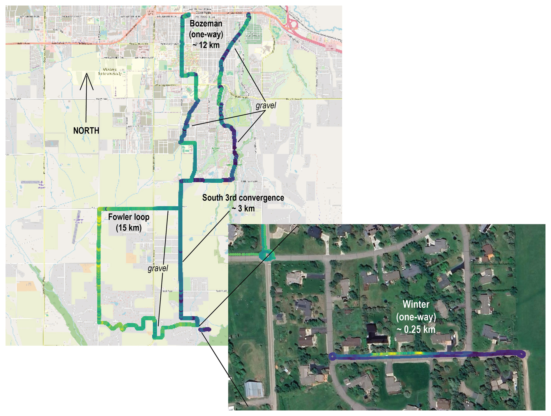
Figure 1 Routes of bicycle measurements of surface properties around clockwise Fowler loop (7 July 2023) or to-and-from Bozeman (6 September 2023) Montana. Routes conveyed in this case via GPS-located measurements of surface temperatures minus air temperatures, with individual records appearing continuous on these scales. Inset shows, at higher resolution, winter walk data along Jade Street, plus typical bicycle loops performed at starts and ends of Fowler loop or Bozeman rides (for further information on start/end loops check Fig. 3). Inset image demonstrates occasional slight mis-registration between ground and satellite position data (addressed in Appendix H). Winter data come from 16 February 2023. Screenshots of data displayed in QGIS software, with background imagery from Open Street Map (© (OpenStreetMap, upper left) or Google Earth (© Google Earth, lower right).

Pavement engineers classify these surfaces as “chip-sealed”: mixtures of asphalt binding materials with stone inclusions. In rare spots, original darker asphalt (with fewer stone inclusions) had not yet received particle-rich chip-seal top coats. Pavement colors, dominated by inclusions of local stones, varied only slightly: gray to darker gray. I rarely rode over whiter concrete surfaces, generally only at recently-constructed intersections or surfaces in downtown Bozeman.

Data presented here came primarily from local county (Gallatin) or urban (Bozeman) roads; they qualify – by width, boundaries and surface or subsurface preparation – as “local roads and streets” under State of Montana definitions (State of Montana Pavement Design Manual, available at https://mdt.mt.gov/publications/manuals.aspx, last access: July 2025). The State of Montana follows US federal pavement guidelines and disseminates materials largely to guide pavement contractors; pavement manuals focus primarily on durability. A pavement engineer might consider asphalt-based chip-sealed surfaces as “flexible” while regarding concrete surfaces as “inflexible”. This data set considers all pavements as impervious from hydrological and thermal perspectives, in contrast to pervious conditions encountered when traversing gravel or grasslands.

Standard 15 km (“Fowler loop”) rides (Fig. 1) included 0.4 km of north-south gravel (“frontage”) road (bounded before and after by north-south paved surfaces) plus 0.7 km of east-west gravel at eastern end of Patterson Road (both marked on Fig. 1). These gravel stretches represent unpaved roads, passable but graded not more frequently than twice or thrice per year. Paths traversed on routes into and back from Bozeman proper (again, denoted in Fig. 1) included crushed rock surfaces eroded only by rare motorized maintenance or by very rare surface water flooding plus short stretches of “single” track through surrounding grass. Winter data over snow-covered roads occurred via the same bicycle and sensors pushed at walking speeds to and fro along snow-covered Jade Street (occasionally labelled as Jade Lane, Fig. 1 inset).

Fowler loop included large road-side trees near the northwest corner and again at the east-west uphill ditch-crossing stretch near the southern terminus. Tree coverage (mostly from conifers or seasonally-varying cottonwood trees) at these locations extended across the roads, imposing shade at almost all hours. Other tree shadows, where present, depended strongly on sun angles; shade extended across both lanes of north-south travel only during early morning or late afternoon hours. Each data record includes precise location and time of day from which users can easily calculate effective sun angles and surface exposures; Sect. 4 conveys details of tree-induced shading. Routes to-and-from Bozeman proper passed through consistently shaded areas near or under creek-side trees. In all cases, data from sky-exposed optical sensors (visible and UV) provided good records of immediate solar exposure.

3 Sensors

I operated all sensors on a single I2S bus managed by a Teensy 4.1 microcomputer. As shown in Fig. 2, sensors (up-looking, down-looking or immersed in flowing air) plus the u-blox GPS unit operated from a box powered via a USB connection, with all sensors exposed to clean air 70 cm above ground surfaces. Up-looking sensors (Fig. 2a) included VEML6030 (visible) and VEML6075 (UV) plus the u-blox GPS antenna. Down-looking sensors (Fig. 2a) included the MLX90614 infrared (IR) surface temperature sensor plus an AS7263 near-infrared (NIR) spectral sensor. Air temperatures came from co-located doubly-shielded SHTC3 and TMP117 sensors (Fig. 2b); the SHTC3 also provided humidity data. Ahead of those sensors, in clean airflow, I operated a FS3000 air flow sensor (Fig. 2b) during 2023. The much-ventilated box housed microcomputer plus u-blox GPS processing board plus a conventional on-off switch. All sensors operated within < 20 cm of each other: total end-to-end length for box plus boom equaled 32 cm. Total bicycle-mounted weight including metal bracket, metal mounting plate, fasteners, bumpers, box, sensors and power and signal wires, remained under 700 g. Users could build copies of this complete sensor set for ≤ USD 300.

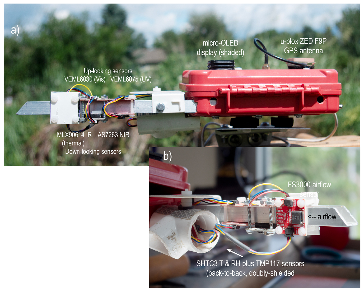
Figure 2 Sensor box showing location of all sensors from left ((a) in direction of bicycle travel) and, closer view, from right (b). OLED display, driven by the microcomputer, displayed three data lines including GPS time, very useful to confirm GPS synchronization and for comparison with Garmin 830 unit at start of each ride. In 2023 I installed an FS3000 airflow sensor (b) to monitor air flows across temperature sensors. Interested users can easily compare Garmin GPS-derived bicycle speeds to FS3000 velocities from these data (Appendix G).

3.1 GPS

I operated a bicycle-specific Garmin 830 cyclometer in standard GPS configuration (Figs. 2a, 3a). After each ride I converted cyclometer data via .tcx format to .csv files. For reasons of low spatial resolution and persistent redundancy, I do not include Garmin cyclometer data with these data files (see Data Description). To provide reference time and location data for all sensors, and to confirm (and out-perform) cyclometer-derived location data, I operated a u-blox ZED F9P GPS as backbone instrument of the sensor box (Fig. 3b and c). I recorded u-blox GPS time and position data along with data from other sensors into composite .csv files.

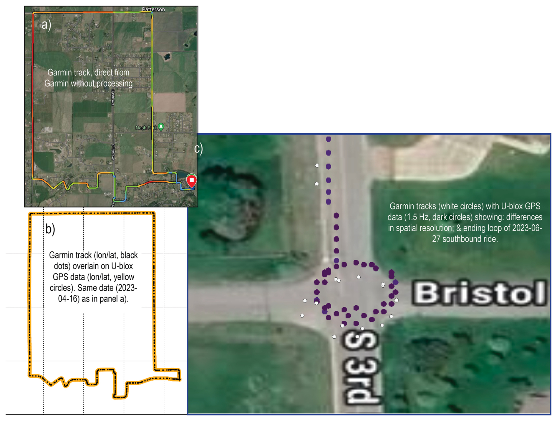
Figure 3 GPS data recorded on Fowler loop ride (16 April 2023) and at termination of southbound Bozeman ride (27 June 2023). Track in panel (a) came directly from a screenshot of Garmin cyclometer data, with no processing or export. Data in panels (b) and (c) came from .csv files relevant to same date, with Garmin cyclometer data exported and converted via .tcx format to .csv while u-blox ZED F9P GPS location and time data (collected at fixed 1.5 Hz recording frequency) came directly from sensor box .csv files. U-blox GPS successfully recorded lane and loop positions at better than 2 m uncertainties during this ride. Users can easily access any sensor data layered on user-selected background in QGIS or other GIS software. Background in panel (c) came from Google satellite image toggled through QGIS; slight offset occurred due to minor mis-registration. Maps © Google Earth.

3.2 Air temperatures

Until November 2022, I used a single high-resolution temperature plus humidity sensor, the SHTC3 unit. After November 2022 I added a second high-resolution TMP117 temperature sensor mounted back-to-back (< 1 cm distance) with the SHTC3, both within a double-layer radiation-protected white-plastic (standard PVC pipe) flow-through chamber (Fig. 2b). I purchased these (and most other) sensors mounted on Sparkfun breakout boards; breakout boards provided onboard processing, conversion to standard units, bus addressing systems, power conditioning, connectability, and easy mounting. I recorded all data from the sensor box (u-blox GPS location and time plus temperatures, humidities, visible and UV light, etc.) into single per-ride .csv files. At temporal resolution of 1.5 Hz, each .csv file held ∼ 4000 records.

I started with a 12-bit Sensirion AG (Switzerland) SHTC3 temperature and humidity sensor. The bandgap SHTC3, intended for consumer electronic temperature measurement applications, provided accuracy of 0.2 °C over the range 0 to +60 °C. I subsequently added a 16-bit TMP117 sensor (by Texas Instruments, USA) specifying 0.1 °C accuracy in the temperature range −20 to +50 °C plus documented compatibility with ASTM and ISO standards for electronic patient thermometers; it functioned as a single-chip digital equivalent of a platinum resistance temperature detector. Both sensors derive from NIST-certified (USA National Institute of Standards and Technologies) manufacturing processes; I include data sheets for all sensors (see Data Description). Figure 4 demonstrates statistically-perfect correlations of TMP117 and SHTC3 sensors configured back-to-back in a protected housing (almost identical to bicycle) under roof-top photovoltaic panels; these data demonstrate consistent reliable operation of both sensors over local air temperature ranges of −30 to 40 °C.

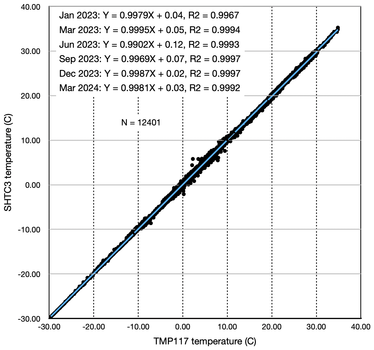
Figure 4 Temperatures as measured by SHTC3 (vertical axis) vs.TMP117 (horizontal axis), across a temperature range of −30 to +40; that range covers most conditions encountered during these bike rides. Data files cover January 2023 through March 2024. Relationship slopes did not deviate from 0.99 while most correlation coefficients equated to 0.999 (with one lower R² value of 0.996). Statistically, SHTC3 and TMP117 produced comparable reliable temperature data.

The SparkFun board hosting the MLX90614 also included an onboard temperature sensor; details and effective resolution of that particular sensor remain vague (not discussed on Melexis MLX90614 data sheet for example). All data files include data from this additional temperature sensor designated as “IR board”, which showed very positive correlations with TMP117 and SHTC3 sensors; readers can use or not use these accessory data. Figure 5 demonstrates additional comparisons of data from SHTC3 and TMP117 sensors: left plot shows a typical Fowler loop ride (on 25 June 2023) using SHTC3 and TMP117 sensors; middle plot shows a ride from Bozeman (on 27 June 2023) again using bike-mounted SHTC3 and TMP117 sensors; and right plot shows identical sensors operating underneath solar panels for the time period 19 to 26 June 2023. These data again demonstrate consistent reliable operation of SHTC3 and TMP117 sensors.

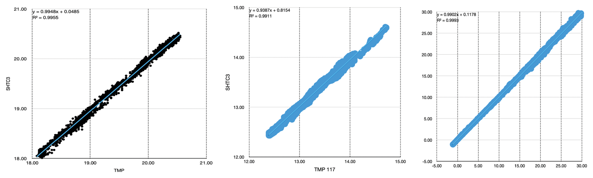
Figure 5 SHTC3 vs TMP117 correlations for three different days. Left: A late day Fowler loop ride, 25 June 2023, after rain. Middle: A morning southbound Bozeman-toward-home ride, 27 June 2023. Right: A weeks' worth of roof-top data. Note smaller 3 °C ranges (18–21, 15–18 °C) for bike rides (left, middle) compared to broad range (−5 to +30 °C) for week-long (right) data. Linear correlation equations and correlation coefficients very high in all cases! Location does not change for roof-top data. Each bike-based data file includes GPS-derived locations and times.

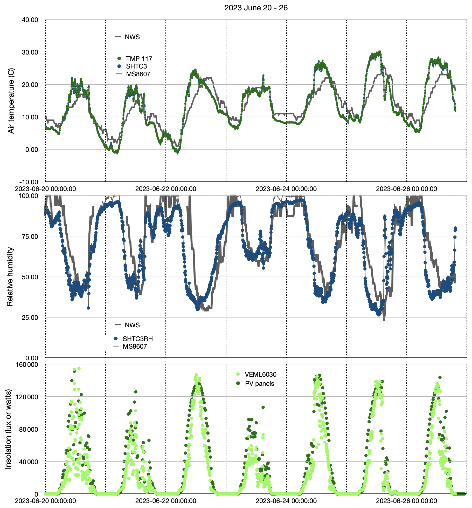
Figure 6 Time series from roof-mounted temperature, humidity and insolation sensors plotted together with temperature and humidity data from nearest NWS station (distant by ∼ 250 m vertical and ∼ 24 km horizontal). Roof-mounted data include SHTC3, TMP117 and MS8607 sensors; the MS8607 sensor (data sheet available) recorded temperature (±1.0 °C over the range −40 to +85 °C), humidity and local atmospheric pressure. This week-long intercomparison also included a fully-exposed VEML6030 (identical to bike-based unit) mounted parallel to photovoltaic panels, plus 15 min power records (via SolarEdge web-based interface) directly from photovoltaic panels (details in Appendix F).

Figure 6 shows time series of air temperatures, relative humidities and insolation over the week 20–26 June 2023 (also shown in right plot from Fig. 5) for SHTC3, TMP117, MS8607, VEML6030, roof-mounted photovoltaic panel, and NWS data. Temporal correlations of SHTC3, TMP117 and MS8607 data proved excellent: not distinguishable among three sensors on these scales (top panel of Fig. 6). Correlations with distant contemporary NWS station data also proved remarkably good, particularly when all sensors duplicated – successfully – diel patterns and amplitudes of daily temperature or humidity increases and declines! Figure 6 also demonstrates excellent week-long correlations of roof-top insolation (VEML6030, in lux) with roof-mounted photovoltaic panel power outputs (in watts). Readers will find details of sensor-to-photovoltaic panel comparisons in Appendix F.

3.3 Surface (pavement) temperatures

I measured surface temperature using a downlooking MLX90614 infrared (IR) thermometer on a Sparkfun board that included microprocessor, bootloader, status LEDs, communication ports, etc. The MLX90614 sensor itself, from Melexis (global), operated over the range −70 to +380 °C, with 0.5 °C accuracy over a narrower range of 0 to +50 °C. MLX90614 sensors (data sheet available) allow non-contact temperature measurements in a wide variety of medical and remote sensing applications; abundant reports document applications of MLX90614 to remote sensing of human body temperatures, even to skin-based virus (Covid) detection (e.g. Costanzo and Flores, 2020). With a wide field-of-view (90° for MLX90614BAA), mounted 70 cm above pavement surfaces, this IR sensor measured surface temperatures within a 1.4 m diameter footprint which necessarily included a small portion of the bicycle front wheel. A constant portion of a rapidly-rotating wheel within the sensor field of view should present no interference to measurements of surface temperatures. Starting or ending loops, which showed no statistically-valid perturbations, would have exposed wheel-induced directional or rotation-speed factors. All subsequent analyses of this data ignore that small feature. Figure 7 shows typical output from the MLX90614 IR surface temperature sensor.

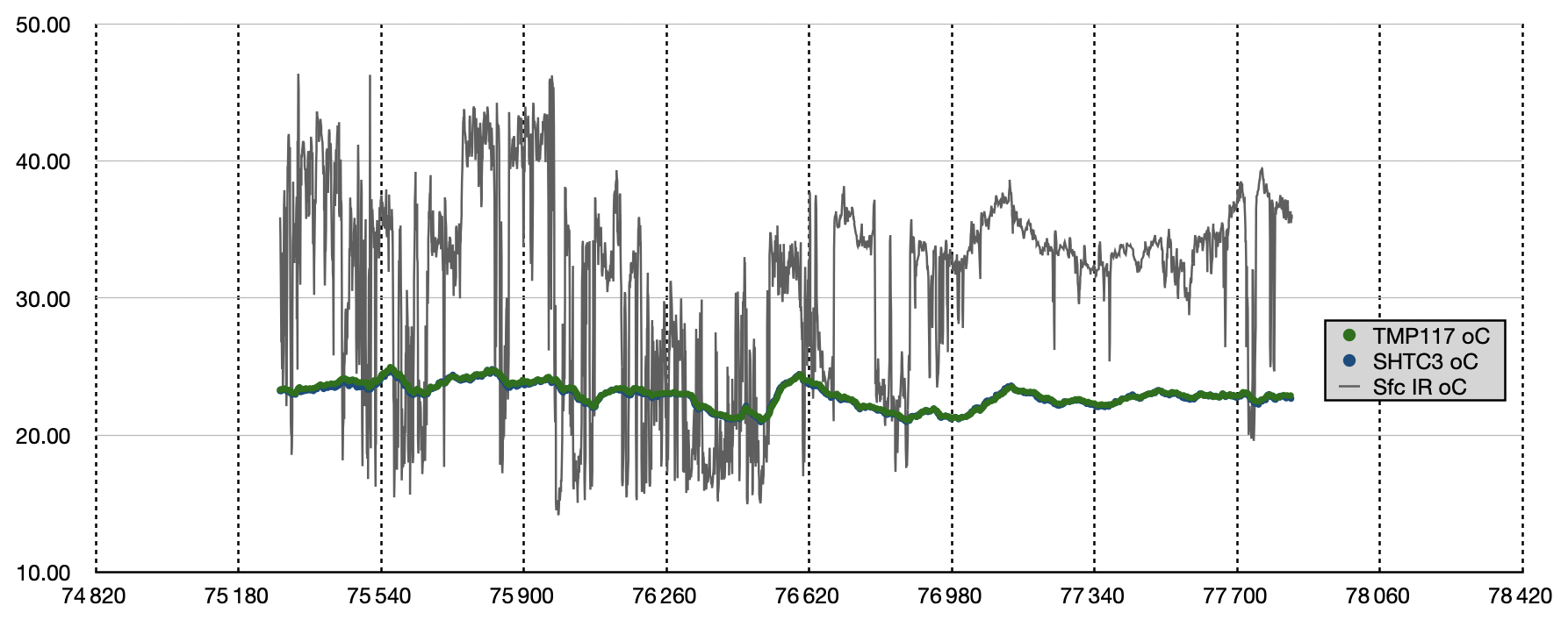
Figure 7 Air and surface temperatures, 6 September 2023. Air temperatures from TMP117 and SHTC3 sensors, indistinguishable in this figure. Surface temperatures from MLX90614 IR sensor. Data collected along same Bozeman southbound (town-toward-home) route shown in Fig. 1. Readers will quickly notice, well within 0.5 °C uncertainty, MLX90614 data showing initial warmer-than-air pavement temperatures, followed by stretches (75 400 to 76 500 s) of shaded gravel paths (interspersed with travel along paved streets), succeeded eventually by long stretch along south 3rd with, again, warmer-than-air surface temperatures; short isolated patches of deep shade exist near end of the ride, inducing small patches of cooler IR surface temperatures. Gridlines along x axis mark 6 min time stretches, each containing roughly 500 recorded data points.

3.4 Relative humidity

Data sets include relative humidity (RH) values from the Sensirion SHTC3 sensor: +2 % RH over humidity range of 0 % to 100 % (details in SHTC3 data sheet). Humidity data from this bicycle-mounted sensor, along with humidities reported by roof-mounted SHTC3 (and MS8607), provided temporal and amplitude verification when compared to humidities measured at NWS station. As for air temperature data, SHTC3 RH data in comparison with MS8607 data and NWS data showed excellent magnitudes and timing of diel excursions (Fig. 6). Bicycle-based RH data did not prove useful.

3.5 Visible light

Data files include visible light measurements (in lux) from a 16 bit VEML6030 ambient light sensor from Vishay Semiconductors (USA), manufactured for use in consumer mobile devices and displays. With a broad thermal operation range (−25 to +85 °C), the VEML6030 records light of wavelengths 450 to 750 nm with a response curve nearly identical to that of human eyes. For outdoor use I operated the VEML6030 with a gain of 0.125 and an integration time of 25 ms; at these settings VEML6030 measurements typically maxed out at 160 000 lux. I compared bicycle-mounted VEML6030 data to data from an identical fully-exposed VEML6030 sensor, mounted beside and parallel to roof-top photovoltaic panels, as well as to 15 min records of power generated (watts) by the photovoltaic panels (Fig. 6; intercomparison details in Appendix F). Roof-mounted VEML6030 data compare very well with photovoltaic data (Fig. 6) while VEML6030 data from the bicycle provide useful records of insolation during a ride including immediate data on tree- or rider-induced shading (Fig. 8, Appendix F).

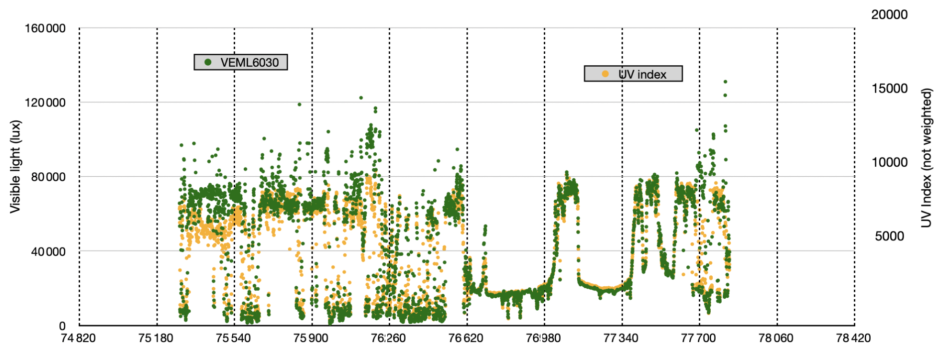
Figure 8 Bicycle-measured visible (VEML6030, in lux) and ultraviolet (UV, VEML6075, in uw cm⁻²) data on 6 September 2023, along same southbound route as shown in Figs. 1 and 7. Visible and UV sensors show very clear responses to time-dependent light increases (gradual increase of “maximum” levels from 75 000 lux to greater than 80 000 lux), to intermittent full sun and full shade, to clouds (rounded transition edges), etc. Isolated patches of deep shade near end of ride show very clearly in these data. Time axis parameters identical to those in Fig. 7: UTC, GPS seconds, 6 min (∼ 500 records) between vertical gridlines.

3.6 UV light

Data files include ultraviolet (UV) irradiance at two wavelengths (UVa 365 ±10 nm and UVb 330 ± 10 nm) from Vishay Semiconductors VEML6075. This unit operates from −40 to +85 °C while allowing users to combine UVa and UVb into a numeric UV Index (Fig. 8). Please note: UV index data shown here do not include wavelength-dependent weighting factors nor susceptibility factors. These basic data remain valid and useful, particularly as back-up to and confirmation for VEML6030 Vis data; users may calculate UV exposures for specific locations and elevations, corrected for local cloudiness, according to appropriate national or international guidelines.

3.7 Near-infrared spectral measurements

Data files include red to near-infrared (NIR) absorbance data from 610, 680 and 860 nm, all with 20 nm full-width half-max (FWHM) spectral resolution. These data come from a downlooking stable AS7263 sensor unit from ams AG (Austria) which detects sunlight reflected from underlying surfaces. Users can evaluate data at 610 and 680 nm to determine slopes of red end of visible spectra or to estimate overall spectral shapes. In contrast to many surface (including bicycle) measurements which require users to extrapolate downwards from periodic satellite data, users can use these data to calculate upwards; they can use data at 680 and 860 nm to calculate an equivalent in situ normalized difference vegetation index (NDVI, see Appendix F for calculations) with implications for remote sensing measurements over roads and other surfaces. Normalization during NDVI calculations plus comparisons with time of day and incoming sunlight (VEML6030) can prove useful in understanding spectral data. Figure 9 shows, again for southbound ride on 6 September 2023, calculated NDVI (as described in Appendix F) compared with total sunlight (from VEML6030); NDVI calculations covered, on this particular ride, paved, graveled and grassy surfaces.

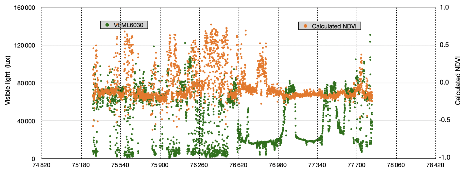
Figure 9 Normalized difference vegetation index (NDVI) calculated from spectral data at 680 and 860 nm, along southbound bicycle ride on 6 September 2023. Lux (insolation) data from VEML 6030 exactly as in Fig. 8. NDVI from spectral wavelengths measured by AS7263. Normalization results in relatively-flat slightly negative NDVI values over impervious surfaces with strong positive excursions in shaded areas. x-axis exactly as in Figs. 7 and 8, with gridlines every 6 min.

3.8 Microcomputer, software and temporal resolutions

I used a 600 MHz ARM Cortex-M7 Teensy 4.1 (https://www.pjrc.com/teensy/, last access: July 2025) to run all systems and to collect (on microSD card) all data; this Teensy 4.1 microprocessor provided accessibility and reliability to the full system. I used standard C$++$ libraries (from Sparkfun in support of each sensor or from GitHub likewise) compiled within the Arduino IDE programming environment. In many cases, after interconnecting the full suite of sensors, I could run sensor-specific example codes to check operation of each sensor. In the case of the MLX90614 sensor, I used a library from Adafruit (likewise available on GitHub) in preference to the Sparkfun library. A typical data file from a Fowler loop data ride, collected at 1.5 Hz, amounted to roughly 400 kB (4000+ records) across 16 variables (15 without TMP 117 before 18 November 2022): GPS seconds, lon and lat from u-blox GPS; six records (five without TMP 117) from temperature and humidity sensors [T_sfc-T_air calculated]; seven data records from optical sensors [including calculated NDVI]. As already mentioned these as-recorded data include no averaging, interpolation or other data processing.

Data sheets show that sensors had potential to operate – on their own, isolated from others – faster than several Hz. Even the u-blox GPS unit advertised raw position update rates of 20 Hz or faster. In this configuration, however, after sensors received suitable warm-up, performed – when necessary – various boot-up steps, and as the moving u-blox GPS maintained adequate synchronization to transmitting satellites, actual recording times included individual sensor signal processing, transfers via I2C bus, writing times via a microSD drive, etc. Combined processing steps resulted in total data record processing times very close to 1.5 Hz. By adopting new libraries and improving prior codes, I added (after bike crash on 18 November 2022) two new sensors without impact on overall processing speeds; later code refinements allowed data recording speeds of closer to 2 Hz (e.g. by September 2023). Applied uniformly, 1.5 Hz at 5 m s⁻¹ implied spatial resolutions near 4 m. Bicycle speeds varied, particularly descending versus ascending, so GPS-based time and location data as trigger for each sensor-based record provided actual spatial resolutions. As demonstrated in legend to Fig. 7, in e.g. Figs. 13, 14, 16, Appendix F, and in demonstration video (https://youtu.be/nMjBFbXxNWU, Carlson, 2025h), these data at these spatial resolutions allowed easy determination of surface features and shade along impervious or pervious roads, streets, lanes, paths, etc.

3.9 Winter-time walking data

During winter, with snow-packed or icy roads, I walked same bicycle carrying exactly the same sensor box and using same Garmin 830 cyclometer along Jade Street. This short stretch of not-much-traveled rural pavement included hard-packed (by vehicles or snowplows) snow and ice, particularly at the tree-shaded east end, occasional occurrences of fresh untracked snow, and melting wet or bare pavement in sun-influenced central sections. Users should examine various still images (see Data Description in Sect. 7), Appendix G and demonstration video (https://youtu.be/nMjBFbXxNWU, Carlson, 2025h). I completed westward-then-eastward walking deployments, generally covering nearly 0.8 km with loops at both ends, within 10 min. In all cases I collected data identical to bicycle rides. On one occasion (16 April 2023) I walked along Jade Street then rode around Fowler loop. I also encountered snow or ice during “regular” bicycle rides but generally in small patches easily avoided or surmounted. On only one occasion (18 November 2022) did I fall due to slippery surfaces. During recovery from that event I added TMP117 sensor and updated acquisition codes.

4 Data uses

Data presented here cover 110 complete rides around Fowler loop (excluding interrupted partially-completed ride on 18 November 2022), 61 rides to or from Bozeman proper, plus 31 winter-time walks along snow-covered Jade Street. Readers will quickly notice three distinguishing features:

1. In no case did air temperatures respond to surface temperatures. When warm or cool patches occurred in air temperature records (such conditions occurred – rarely – after dark, see data for 15 June or 23 August 2023), atmosphere features occurred without impact on surface temperatures. Insolation (or, conversely, tree-induced shading) forced surface temperatures while – as a general case – air temperatures remained largely immune to surface influences.

2. Gravel (pervious) surfaces proved cooler than paved (impervious) surfaces. At periods of maximum impervious surface temperatures (e.g. ≥ 25 °C), with impervious and pervious surfaces both exposed to full insolation, graveled surfaces proved at least 5 °C cooler.

3. Tree-induced shading, particularly dense multi-hour and multi-season shade, resulted in cooler surface (paved as well as graveled) temperatures. Due to generally dry climate in this portion of Montana, where trees often grow along (and provide shade to) streams or irrigation ditches, systematic data such as these will help sort shade and waterway influences.

I offer examples intended to stimulate questions, explorations and replications. I address a series of validation questions.

• 1.

  How did these data compare to “official” NWS data?

• 2.

  How did bicycle data compare to local roof-based data?

• 3.

  What maximum and minimum T_sfc-T_air occurred? When, where and why?

• 4.

  How did gravel surfaces differ, thermally, from paved surfaces?

• 5.

  What happened in fully (day-long) shaded areas? What happened when shading occurred for only parts of a day?

• 6.

  What happened as snow or ice accumulated, compressed and then melted?

Prospective users might raise additional questions about durability of specific sensors, about environmental conditions at a fixed location as a function of season or time of day, or about variances (or, not) along particular stretches according to surface type or canopy coverage. These data provide effective baselines for subsequent investigations; sensor outputs proved repeatable and reliable over multiple years (Appendix H).

4.1 Validation of these data against US Climate Reference records

As mentioned (legend to Fig. 6), the “nearest” long-term “official” climate-quality data come from a USA National Weather Service (NWS) station at Bozeman airport, 24 horizontal km and 250 vertical m from Jade Street. Specific bicycle routes, at their northern-most extents, might have modified those distances by ±10 km. Figure 10 compares bicycle-derived air temperature data, collected bidirectionally along south 3rd Avenue, to “climate-quality” data from the NWS station. Readers should extract two conclusions:

• This bicycle-sensor temperature combination successfully recorded data from March to November (with a few data-gathering rides in DJF as permitted by weather) with outcomes very close to nearby NWS data. As intended, bicycle walks in February and March of 2023 added useful air temperature data during “winter” seasons. Considering brief collection periods of bicycle-based data, often gathered during maximum diel illumination periods, their correspondence with multi-year climate-quality data (one of only three such NWS data sites in Montana), particularly between daily mean and daily maximum records, proved remarkably good (Fig. 10).

• Temperature sensors on the bicycle reproduced local “official” annual data with very high fidelity. Extracting data recorded along a frequently-ridden 3 km stretch of open road, thereby avoiding deeply shaded or graveled surfaces, produced remarkable correspondence to weather service records.

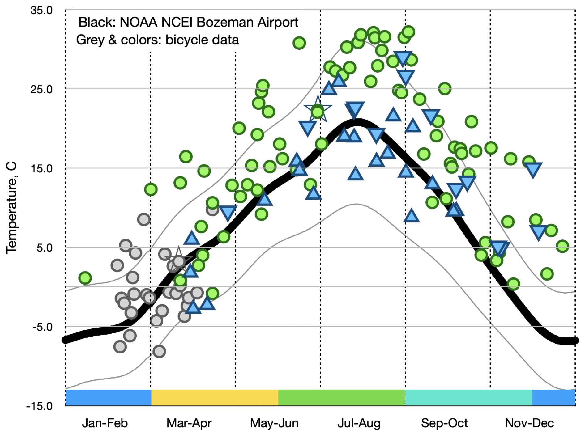
Figure 10 Average (over 8–15 min) air temperatures from bicycle sensors compared to climate-quality data from nearby US NWS station at Gallatin (Bozeman) Airport. NWS data from NOAA NCEI, 27-year average (1991–2018, USW00024132, https://www.ncei.noaa.gov/access/us-climate-normals/, last access: July 2025) quality-controlled air (2 meter) temperatures showing daily averages (central black line) plus daily maximum and minimum (upper and lower narrow black lines). All non-winter data come from identical route along south 3rd Avenue (see Fig. 1): green dots from Fowler loop rides (clockwise, e.g. north-to-south along south 3rd, in all-but-one case) while blue triangles indicate Bozeman rides (upward-pointing triangles indicate northbound rides, downward-pointing arrows indicate southbound rides). Triangles often occur in pairs: northbound (to town) ride followed by southbound (return from town) ride. Gray dots indicate winter-time snow/ice walks. Stars indicate dates of maximum surface temperatures (> 31 °C warmer than air temperatures on 30 June 2022, starred green dot) and minimum ($<-$14 °C relative to measured air temperatures on 23 March 2023, starred gray dot). Colored bars along horizontal access denote climatological periods: December–January–February (DJF), March–April–May (MAM), June–July–August (JJA) and September–October–November (SON).

Acknowledging excellent sensor-to-sensor intercomparisons (e.g. Figs. 4 and 5) plus very positive temporal correspondence of bicycle sensors with local roof-mounted and distant appropriately-housed NWS sensors (e.g. Fig. 6) over weeks of data collection times, one concludes that these bicycle-carried sensors provided highly accurate temperature measurement capabilities, at specified sensor accuracies. Minor vertical corrections (e.g. < 1 m for bicycle compared to “official” 2 m heights for NWS data) probably prove inappropriate in these cases, particularly in view of short durations of bicycle-based data gathering plus interventions by other (bicycle motion, horizontal distance, elevation offset, shading, surface type) factors, in addition to constantly variable distances between bicycle and NWS station; any such minor “correction” would only improve already-good correlations. Location-based elevation changes, e.g. drop of approximately 50 m from SE to NW corners of Fowler loop or of greater than 120 m to many locations in Bozeman proper, probably had greater impact than specific bicycle-based sensor heights. In these locations and for these types of deployments, additional publicly-accessible validation data prove scarce at best, essentially non-existent. More recent climate warming impacts, as those emerge within longer-term NOAA NWS records, will also improve intercomparisons. I address longer-term repeatability and reliability of these measurements in Appendix H. I conclude: use of these sensors for bicycle-based measurements of air and surface temperatures proved reliable and appropriate. Users can easily access these data to confirm or contradict.

4.2 Intercomparison of bicycle-based data “snapshots” to daily and seasonal patterns of insolation, including from roof-top photovoltaic panels

Figure 6 demonstrated excellent temporal and amplitude correlations between roof-based sensors (identical to bicycle-based sensors), NWS sensors, and roof-based photovoltaic panels, across a week of 5 min (rooftop sensors) and 15 min (NWS) data. In general, bicycle data came from rides during hours of 10:00 to 16:00 or 17:00 local time; I often rode early toward town but rarely started a ride before local dawn and rarely rode after local dusk. By compiling rides to/from Bozeman with Fowler loop rides I managed to cover most daylight hours, producing excellent temporal correlations of bicycle-measured insolation maxima with nearby roof-top solar power generation records (Fig. 11). Appendix C shows similar ride distributions with consistent diel patterns for March–April–May (MAM, 36 total rides across 2022 and 2023, Fig. C1) and September–October–November (SON, 56 rides from 2021–2023, Fig. C2). During December–January–February (DJF) of 2022 and 2023 I rode only five Fowler loops plus four rides to or from Bozeman. Figures 11 and C2 hint at behavioral patterns: Bozeman rides early with most Fowler loop rides occurring later. Insolations recorded by bicycle-based sensors at 1.5 Hz rarely exceeded 15 min roof-top power generation data; bicycle-based data lower than maximal roof-top power data indicated cloudy, shaded or (rarely) rainy conditions. I gathered valid data using this bicycle over most daylight hours during most seasons.

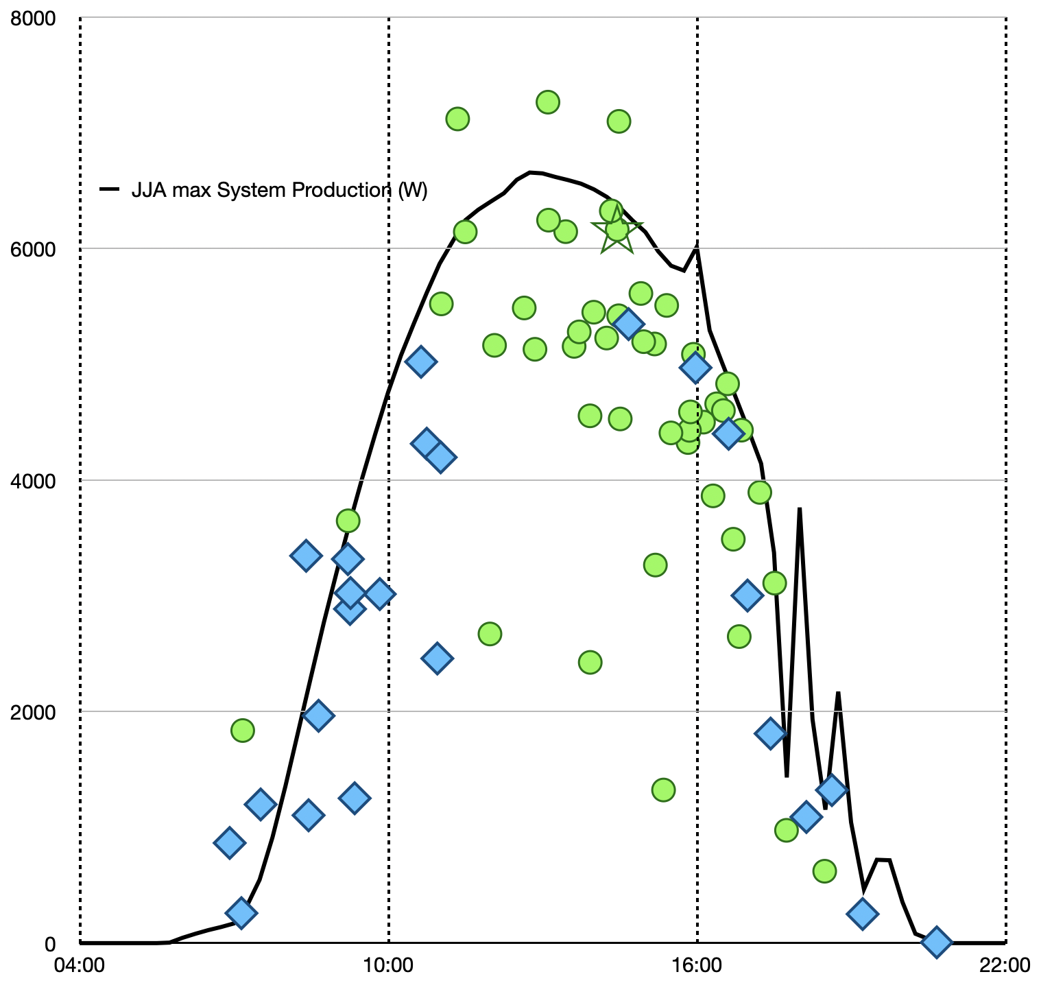
Figure 11 Maximum illumination values from bicycle-mounted VEML 6030 sensor sorted by start times for bike rides around Fowler loop (green dots) or to-from Bozeman (blue diamonds), compared to maximum power records from roof-mounted photovoltaic panels, for all June–July–August (JJA, climatological northern hemisphere summer) data from 2022 and 2023. Photovoltaic data, recorded as 15 min power output summaries (solid black line), came from 23 July 2023; those data show typical morning insolation followed by afternoon cloudiness. Bicycle data represent maximum illumination data, in lux, measured during full rides, e.g., not restricted to oft-ridden stretch of pavement on south 3rd Avenue; data gathered from shaded stretches of pavement should have no impact on ride maxima. Star (on green dot) highlights the ride on which maximum T_sfc-T_air occurred: > 31 °C on 30 June 2022.

4.3 Average, maximal and minimal surface versus air temperatures

T_sfc-T_air values, covering more than 600k individual GPS-located records, including data collected during winter walks along Jade Street, ranged from a low near −14 °C (Jade Street walk) to a high of greater than 31 °C (Fowler loop ride). Parsed by date and time of bicycle ride/walk, over a total of 202 bicycle-based rides and walks (171 Fowler and Bozeman complete rides plus 31 winter walks along Jade Street), 45 (22 %) had mean T_sfc-T_air temperatures > 15 °C (means cover all data points recorded within a ride, including partial shade, deep shade, wet spots, etc.) while 31 (15 %) had mean T_sfc-T_air temperatures below 0 °C (percentages and averages calculated from spreadsheet table as described in Appendix B). Figure 12 demonstrates frequency distribution of mean T_sfc-T_air values across September 2021 to October 2023. Again, mean data cover full rides including all types of surfaces: predominantly impervious pavement but also pervious gravel and grass-lined tracks, gathered in full sun or shade, including snow and ice, etc. Clearly, warmer temperatures of all surfaces (surface temperatures warmer than air temperatures) dominate; an overall mean of all ride-based means equates to 7.76 °C (Fig. 12). Such dominance conveys partly-relevant information however: one must also account for percent impervious versus pervious surfaces plus effects of day-long or intermittent shading. One can report, with confidence, that surface temperatures minus air temperatures covered a relatively wide range in these Montana data, converging around average warmth for all surfaces at all seasons of roughly 8 °C.

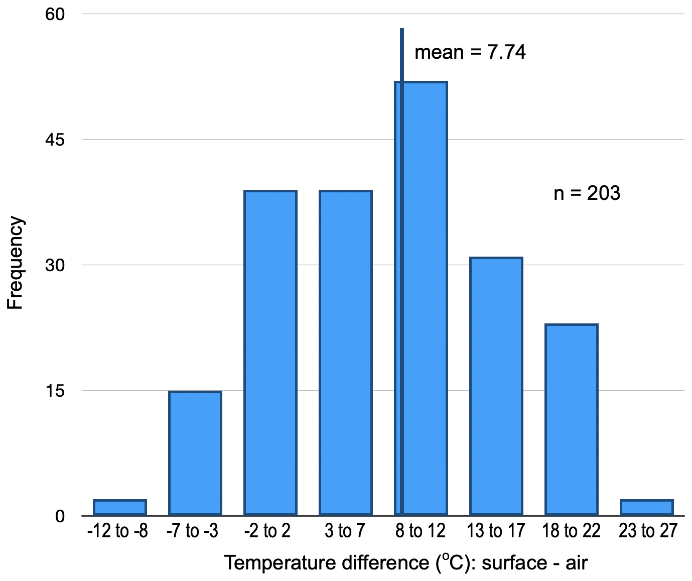
Figure 12 Frequency distribution of mean T_sfc-T_air data for 202 data records: 171 Fowler loop or Bozeman rides plus 31 winter-time walks along Jade Street. Column labels rounded to integer units (−2 to 2); actual sorted values cover 5 units (−7.5 to −2.5, −2.5 to 2.5, 2.5 to 7.5, etc.) Mean of all data = 7.76 °C (solid line).

Maximum T_sfc-T_air (∼ 31.0 °C) occurred on 30 June 2022 just after turning east on Patterson Road near the NW corner of Fowler loop (Fig. 13, left). Maximum surface temperature (> 30 °C) occurred again in that same location (Fig. 13, left) during a subsequent CCW ride along the identical route; very warm surface pavement on that CCW ride also occurred west of a deeply-shaded area of cool surface temperatures near the SE corner (Fig. 13, right). Long unshaded stretches of both Fowler Road and south 3rd showed very warm T_sfc-T_air temperatures, whether riding CW or CCW, on that particular day. Table 1 presents ranges of air temperatures (T_air), pavement surface temperatures (T_sfc) and differences (T_sfc-T_air) recorded on that warm day compared to similar data collected on colder (April, May) rides. T_air absolute values and small ranges seemed typical for time of year. In all cases T_sfc, and consequently T_sfc-T_air, showed much larger ranges, without response to nor influence on air temperatures. Ridden either direction (e.g. any panel of Figs. 13 or 14), surface temperatures averaged almost 25 °C warmer than relatively stable air temperatures of 23–24 °C on that day; no combination or direction of advective air movement (wind) could have caused pavement temperature patterns. Actual pavement surface temperatures greater than 50 °C occurred frequently while air temperatures showed no similar excursions (Table 1, time series in Fig. 14). Taking into account paved, graveled and shaded surfaces, JJA average surface increments of 21 °C over averaged air temperatures of 25 °C resulted in average maximum surface temperatures of 46 °C for those summer rides. In a relatively rare example of direct radiatively-measured surfaces, Pomerantz et al. (2000) reported similarly warm surface temperatures for one warm afternoon near Berkeley, CA.

Data from a Fowler loop ride on a cooler (April) day, with air temperatures between 2 and 6 °C (Table 1), for conditions annotated as “windy” (Appendix B), showed, again, warm pavement patches on Patterson Road a few meters after the eastbound turn from Fowler Road. Despite substantial differences of both air (5 °C) and pavement (11 °C) temperatures compared to warmer June data (Fig. 13), warm patches of pavement and cooler shaded patches appeared in approximately similar locations. Again: why?

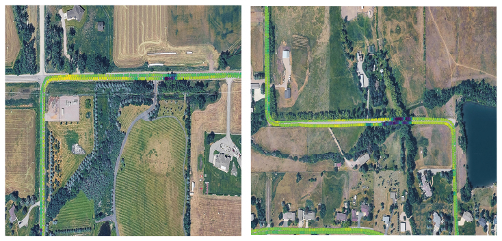
Figure 13 Surface temperatures minus air temperatures (= T_sfc-T_air) for rides clockwise starting at 73 269 s UTC (∼ 13:35 local time) then counter-clockwise starting immediately after at 76247 s UTC (∼ 14:18 local time), around Fowler loop on 30 June 2022. Data (color) scales, (particularly for temperature maximum) nearly identical in both cases (see also Table 1). In each plot, upper track in east-west direction records data from second counter-clockwise ride. In all cases, location of maximum surface warming (T_sfc-T_air > 30 °C) occurred close to patches of cooler surface temperatures in “permanently” shaded areas. Background data © Google Earth.

Table 1 Sensor values for: cold early April 2022 bike ride (annotated in my notes as “windy”, see Appendix B); for 30 June 2022 rides (CW followed by CCW, see also Figs. 13 and 14); and for 14 May 2023 ride again annotated as “windy”. All values rounded to whole integers. Absolute values and ranges of T_air on all days look as expected compared to local NWS data and to other sparsely-available bike data of a few months' duration (e.g. Ziter et al., 2019). T_sfc and, as a consequence, T_sfc-T_air always had broader ranges and, generally (by season) greater values. Users can access and compile similar summaries for all rides on all dates.

One can easily calculate air or surface mean temperatures, time-of-day variations, insolation, etc., for any ride or type of surface (gravel, shaded) over a very broad range of weather conditions (Figs. 10, 11, examples in Table 1). Users might choose to focus on insolation impacts on surface temperatures over any of several full-sun stretches (often ≤1 km in length each with ∼ 200 records) northbound on Fowler (as part of Fowler loop), on north- or southbound stretches of south 3rd Avenue (e.g. chosen from Fig. 1 using information from Appendix B), or – in more-shaded or partly-urban settings – intermediate on north- or southbound Bozeman rides (e.g. Fig. 15). Data from start or end loops gathered on nearly every ride (e.g. Fig. 16 from 4 October 2022) prove that bicycle direction made no difference to measured air or surface temperatures; users can easily confirm absence of dependence of T_sfc-T_air (or, consequently, of surface or air temperatures) on bicycle speed and direction for all loops and all rides.

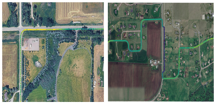
Figure 14 Left panel: Surface warming data (T_sfc-T_air) from CW Fowler loop ride on 9 April 2022. Absolute values and ranges for T_air, T_sfc. and T_sfc-T_air given in Table 1; weather clearly cooler than 30 June example discussed earlier. Despite diminished scale (0 to 11 °C, from Table 1), surface temperature patterns again show warm spots (≥10 °C) on Patterson Road, just after eastward turn from Fowler Road. Right panel: clear example (from ride on 14 May 2023) of cooler surface temperatures on gravel, with “normal” pavement temperatures on adjacent east and west road sections. Background data © Google Earth.

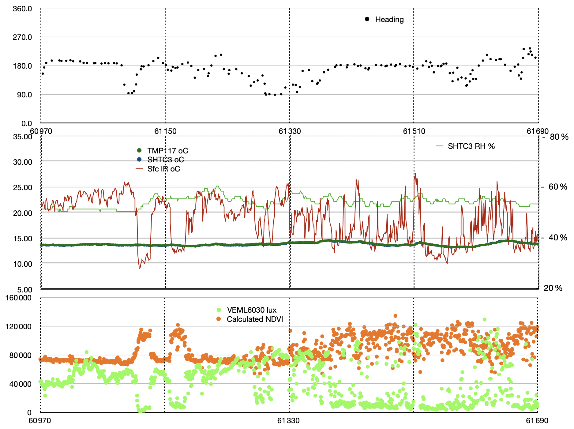
Figure 15 12 min time series of heading (Garmin), T_sfc (MLX90614), T_air (SHTC3 plus TMP 117), relative humidity (SHTC3), visible light (VEML6030), and NDVI (calculated from) measured along a southbound ride from Bozeman, 23 May 2023. Centered at roughly 10:00 a.m. local time, vertical gridlines occur every 3 min, with approximately 85 valid measurements each minute. Predominantly a gravel (pedestrian) path with intermittent shade and sun, chosen to demonstrate fast response of sensors amidst relatively complex vegetation. Users can generate similar plots to support examination of any stretch of any ride. Relative humidity (light green line, center plot) demonstrates RH impact: minimal.

Minimum T_sfc-T_air temperatures dropped below −14 °C (relative to air temperatures of closer to 8 °C) over snow-covered surfaces during a Jade Street walk on 23 March 2023 (Fig. 16). Data from this particular walk demonstrated colder surfaces at snow-covered distal ends of Jade Street with warmer surfaces occurring in melted bare-pavement central regions (Fig. 16). The short introductory video (https://youtu.be/nMjBFbXxNWU, Carlson, 2025h), in addition to presenting brief examples of gravel, wet spots, and shade, shows winter conditions on paved surfaces: snow coverage, cleared areas, local influences of snow types and persistence. Taking all Jade Street walks together, data showed −3.2 °C mean T_sfc-T_air for February 2023 (15 walking data measurements) but 1.9 °C mean T_sfc-T_air during March (16 walks). Average T_sfc-T_air maxima for those months amounted to 5.1 °C for February, 12.1 °C for March. Average minima amounted to −7.5 °C for February, −7.9 °C for March (including −14.8 °C as already noted for 23 March 2023). These data confirm a basic Jade Street pattern: cold surface temperatures at distal (especially eastern) ends, with patches of melted and occasionally dry impervious pavement covering expenses along central areas.

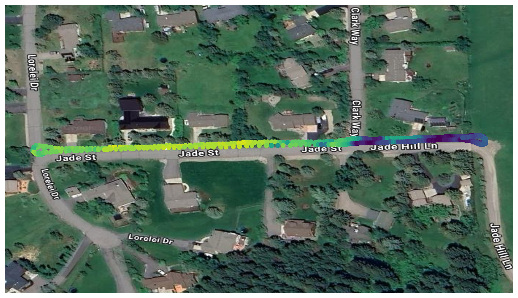
Figure 16 T_sfc-T_air as measured by bicycle while walking along Jade St on 23 March 2023. Data from QGIS analysis include toggled layers of background imagery. Background data © Google Earth.

4.4 Impacts of gravel

Graveled stretches proved distinctly cooler (evident in Figs. 1, 7, 14, and in demonstration video), during Fowler loop circumnavigations (frontage gravel sections along south 19th St and eastern Patterson Road, e.g. Figs. 1, 14) as well as for shorter intermittent gravel sections encountered on to/from Bozeman rides (Figs. 1, 7). Data for both CW and CCW directions (Fig. 14a, b) collected on 30 June 2022 confirm this persistent pattern of cooler surface temperatures (relative to invariant air temperatures) over graveled surfaces.

As demonstrated in Fig. D1 (compare to Fig. 14) spatial patterns of surface warming, shade-induced cooling, cooler gravel surfaces, etc., from a Fowler loop ride on 7 June 2023, particularly cooler pervious graveled surfaces and cooler surfaces in the presence of persistent shade, proved very repeatable. Graveled surfaces often proved ≥ 5 °C (occasionally up to 10 °C) cooler than adjacent impervious pavements, without corresponding decreases in air temperatures.

4.5 Impacts of solar insolation plus persistent versus intermittent shading

Prior work identifies light (solar insolation) as forcing function for surface heating over impervious surfaces: following pavement engineering examples (e.g. in Pomerantz et al., 2000) one might expect insolation to warm impervious surfaces (roads, in this case) which in turn warm overlying atmosphere. Although the second step (pavement warms atmosphere) never emerged from these data, bicycle-based data strongly support the initial step: sun heats pavement. Figure 17 shows positive relationships between maximum insolation and maximum T_sfc-T_air. Figure 18 confirms this insolation-forced pattern: tree-induced shading caused spatially-confined surface cooling. Increased sunlight, for a few hours at least, induced sharper shadows (Appendix E); these results proved consistent and repeatable during multiple rides across multiple seasons among a wide variety of sky conditions. These data, gathered primarily over chip-sealed rural roads, cover a modest range of pavement albedos (e.g. by definitions and examples in Pomerantz et al., 2000) but, according to those same authors, variations in surface albedo of “natural” pavements induced only about 0.5 °C in surface warming or cooling, small to insignificant among these observations. In their immediacy, these measurements do not record insolation occurring hours or days previously or subsequently. For the most part, these data suggest relatively rapid surface responses, certainly within one or two hours for heating or cooling. None of these data demonstrated persistent heating patterns that might lead to heat island effects.

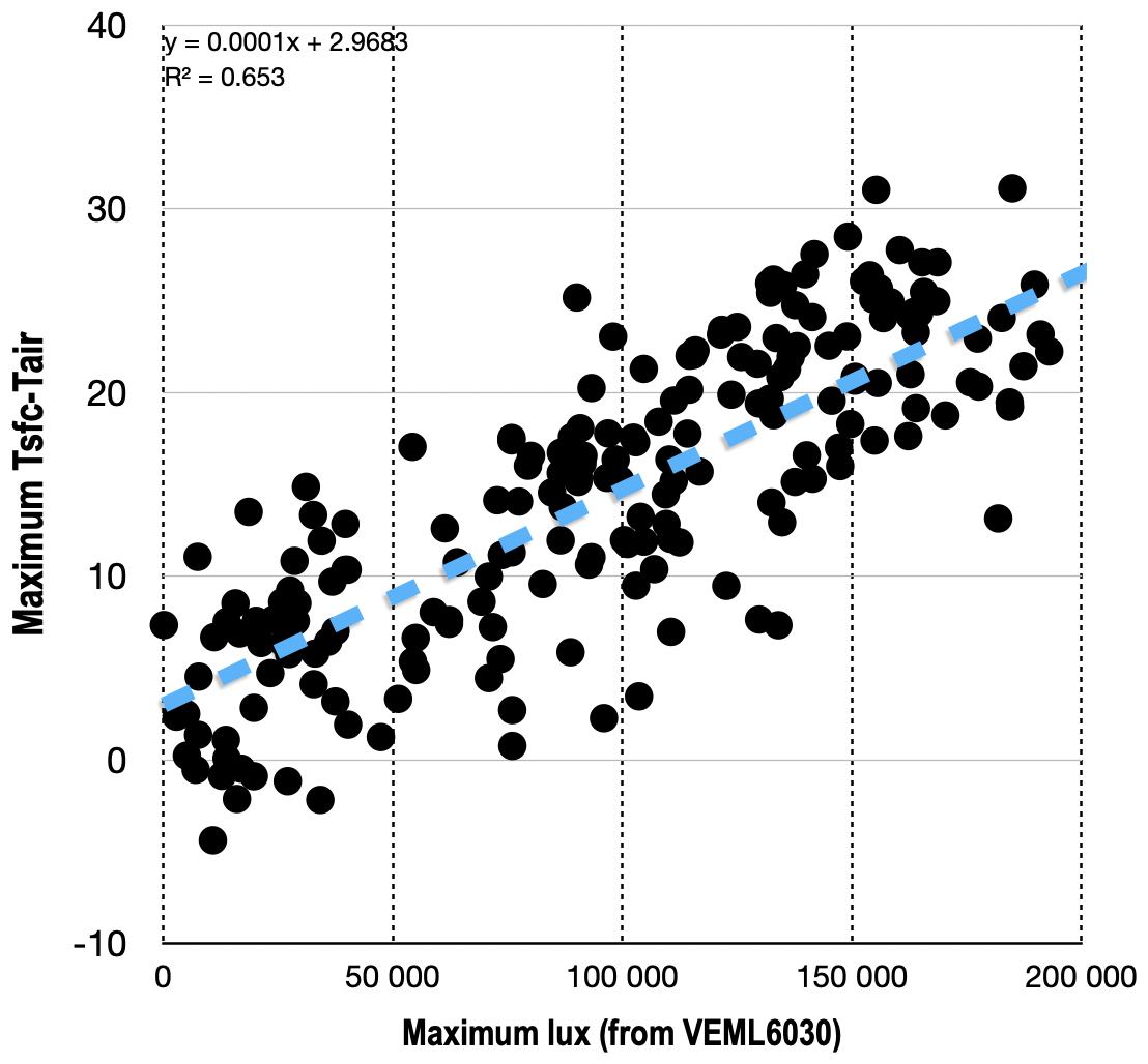
Figure 17 Maximum per-ride T_sfc-T_air (°C) as a function of maximum insolation (lux), for all bicycle rides. Most rides include gravel, shade by vegetation and bike or rider infrastructure, etc.

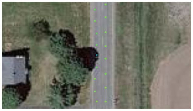
Figure 18 Data from CW and CCW Fowler loop rides on 30 June 2022, demonstrating shade-induced cool surface temperatures measured during CW loop (left track along west lane) followed (less than 20 min later) by identical but non-shaded measurements during CCW loop (right track along east lane). Image based on identical temperature scales northbound and southbound. Data clearly demonstrate cooling impact extending part-way across road surface during southbound pass while northbound pass – without shade – shows no impact. (Particular Google Earth image as GIS background, recorded under very similar late-day insolation conditions, tends to emphasize this pattern.) Background data © Google Earth.

Insolation measurements via light sensors involve substantial variability induced by spectral units, sensor orientations, cloud cover conditions, sensor sensitivity and susceptibility, human or bicycle-induced shading, etc. Users can explore any aspects of these data or peruse further details in Appendix F.

4.6 Winter conditions

As mentioned, winter conditions at this latitude, elevation and particular location often involve snow-covered, plowed, and iced road surfaces (see for example Fig. G1). Ignoring winter-time pavement conditions thereby consigns substantial fractions of seasonal impervious surface temperature data to obscurity. Instead, these data include same bicycle, same sensors, same types of deployments, albeit gathered by cautiously walking the bicycle back and forth along a relatively quiet section of impervious pavement. Figure 10 demonstrates substantial impact of these walks on seasonal coverage of the overall data set. Figure 16 demonstrates persistent patterns of winter data: cold surface temperatures measured at snow-covered ends of Jade Street with warmer surface temperatures evident in sun-exposed central sections. Users can evaluate any of 31 separate bicycle deployments under winter conditions, covering a range of freshly snow-covered, plowed, then traveled (and, subsequently, iced) surfaces. Video of bicycle combined with overhead drone (recorded in https://youtu.be/nMjBFbXxNWU, Carlson, 2025h) may prove helpful in documenting and understanding snow-covered surfaces.

5 Remaining Uncertainties

Acknowledging that bicycle speeds derived from sequential differentiation of GPS positions will vary slightly with elevation change, riding surface, tire pressure, traffic, surface wetness, rider fatigue, etc., position accuracy of these data depend in part on accuracy of derived GPS positions and, at least for GIS interpretation, in equal part on imaging (satellite) uncertainties; uncertainties occur at a much-finer (meter) scale than users might expect. Users should check individual data carefully to understand GPS errors or image mis-registration factors. Over substantial distances, or in cases where neighboring features supply accurate spatial reference, users should regard GPS errors as small (certainly ≤ 2 m as in Figs. 18, E1a, and E1c), while recognizing possibilities, particularly at these small scales, of visual image position errors due to faulty registration. In a few cases (e.g. Figs. 15 and E1b), users will confront ≥ 2 m of obvious GPS positional uncertainty. We all recognize intermittent possibilities of small (∼ 10 m) GPS errors of short (∼ 10 s) duration. This bicyclist who often depends on GIS advises caution at sharp corners or as bicycle emerges from deep shade into full sun; whenever bicycle GPS data might prove uncertain (e.g. Fig. E1b) or when satellite imagery might prove slightly mis-registered (e.g. in Figs. 3c, 15, 16, E1). Where two GPS data streams agree, as happened most often, particularly on straight open sections of road, I accept GPS position uncertainties of 2 m or less and assign remaining uncertainties to mis-registrations. When one GPS position varies from another and from probable image location, I tend to adopt maximum (2 m) horizontal GPS uncertainties; users will need to make best judgements. Positional uncertainties, whether derived from GPS or imagery, had little impact on any data descriptions above. In general, particularly along straight stretches in full sun, along-track spatial resolution of roughly 4 m will prove easily achievable and quite useful. At present, no freely-available satellite imagery, at any wavelength, coverage or repeat frequency, exceeds 10 m of spatial resolution with data records at better than 1 Hz. As data approach meter-scale spatial resolutions, however, concerns about GPS errors versus image registration errors will prove increasingly relevant.

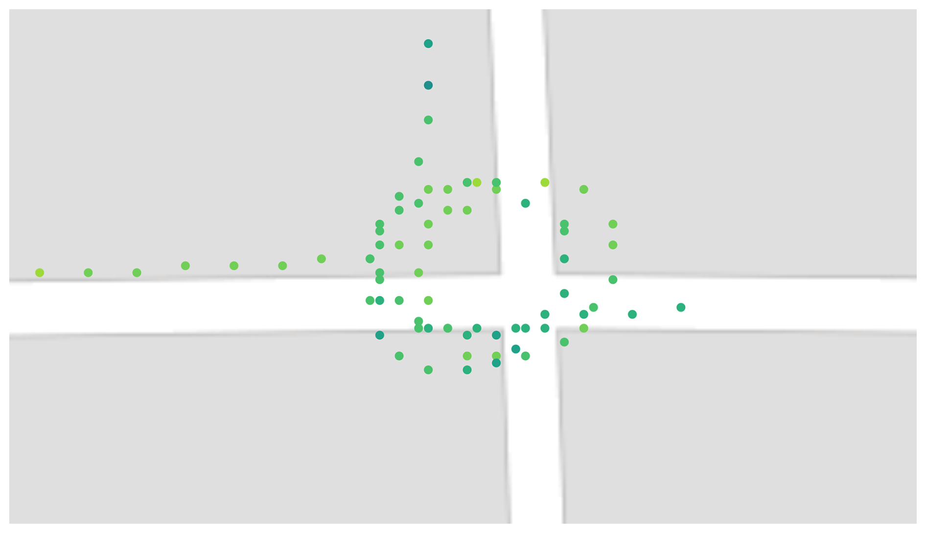
Figure 19 T_sfc-T_air for bicycle loops (start and end) on 4 October 2022. Values (using a single consistent color scale) showed neither directional nor start-versus-end differences. Minimal background comes from Open Street Maps selected within QGIS. Apparent location offset due to misregistration of GPS image? Background data © OpenStreetMap.

Details discussed above proved reliability of air and IR temperatures and light sensors deployed on bicycles for these purposes, plus distinct advantage of recording sensor data synchronously with time- and location-stamped GPS data. As hinted earlier (legends to Figs. 7, 12), users should trust individual T_sfc-T_air data points to at least ±0.5 °C (incorporating uncertainties of TMP117, SHTC3 and MLX90614) over average effective spatial resolution of 4 m.

I include relative humidity data for every data point. As evident from Fig. 6, daytime RH in this dry climate rarely exceeded 50 %; RH data collected on bike rides ranged closer to 30 %. Users can examine, ride-by-ride (e.g. Fig. 15) or collectively, any or all of these data to determine RH impacts on T_sfc or on any other measurement.

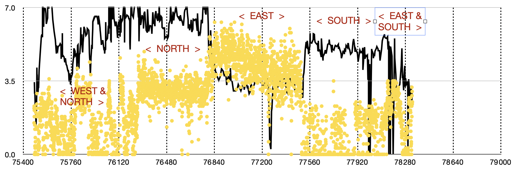
Figure 20 Bicycle speed and air flow (AS3000) data from a Fowler loop ride on 14 May 2023. In post-ride notes I designated this ride as “windy”. Same scale and orientation as other Fowler loop data: clockwise direction, roughly 45 min, each vertical line marks 6 min.

Wind represents a more-complex challenge; I regard wind data from any fixed location at any height with careful skepticism. Measuring air movement from a moving bicycle adds extra – insurmountable – challenges?

Bicyclists always detect wind: opposing or assisting progress or pushing toward or away from road edges. In theory, wind flowing in the same direction as a bicycle-mounted air flow sensor should lower values of air flow. Wind flowing in a direction opposite to bike direction and flow sensor should, by similar logic, cause air flows to exceed bicycle speed. Following that guidance for speed and FS3000 data, one might assume, from Fig. 20, wind from roughly a southwest direction at roughly 3.5 m s⁻¹. But, FS3000 sensor records air flow in a fixed direction oriented to monitor flow over thermistors, not mounted for variable wind directions. Second, wind direction and speed vary widely over 45 min, particularly close to mountains. Third, I do not yet trust operation of FS3000 well enough to understand its response to unhindered air flows. I freely share FS3000 data for every GPS-registered location in all files recorded in 2023; users can test their own solutions. Please look carefully at Fig. 20 before making such an effort. After more than 200 rides in all seasons in all directions, I feel confident that wind played no role in magnitude or patterns of surface temperatures on these wide-open Montana roads. Seasonal factors, surface type (gravel), shade: definitely. Wind? No. Other smarter people than me can attempt to prove me wrong.

6 Implications

Surface temperature patterns observed here (e.g. sun-warmed impervious surfaces, graveled stretches cooler than pavements, shade-induced cooling) represent, individually, no surprises. Other bicyclists, riding at other speeds with other sensors in other locations, could reproduce these outcomes, organise different intercomparisons, conduct different validations, etc. Hopefully, future riders share data!

Cast in terms of radiation or surface energy budgets, these data represent only incoming solar (longwave) radiation, with air temperature as a weak proxy for sensible heat and RH as a weaker proxy for latent energy. Can one make any assumption about outgoing radiation from pavement surface temperatures? Solar panels clearly extract almost 10 watts per hour from incoming longwave; an equivalent of that energy must warm surface pavement? If, as one suspects, these data have little to no value in surface heat budgets, they do nevertheless point out temporal and scalar mismatches between surface heat or energy budgets based, generally, on remote sensing validated by sparsely-distributed flux towers, on generally 8 d averages. Rapid heating and cooling (within minutes to perhaps an hour) proved the dominant time scale of energy exchange. These data from rural roads at 4–5 m spatial scales with nearly 2 Hz time resolution seem beyond the reach of satellite-based averages?

These data do suggest unanticipated features. First, one finds little to no indication of surface influences on overlying air temperature. Heat island effects, much invoked (even as most data remain missing or hidden), evidently require longer heat accumulation or relaxation times, deeper pavement layers with greater heat absorption capabilities, larger expanses of impervious surfaces, abundant reflective buildings, absorbent rooftops, restricted circulation in urban settings, subsurface infrastructure, heating by internal combustion engines, etc; who knows what additional factors convert patterns of quickly warming and cooling impervious surfaces such as observed here to incidences of persistently-warm urban microclimates. As data presented here indicate, researchers exploring urban heat islands using satellite remote sensing will need local high-resolution data. Heat islands remain defined by apparent warmth relative to surrounding rural environments. As Masson et al. (2020) point out: UHI remain complex features of our planet's urban surfaces, without unique or definitive cause. Do UHI definitions refer to some defined rural background? What quantitative temperature differences, urban vs rural? Over which seasons? Might researchers find that they need bicycle data for baselines and for extending observations? That sun warms pavement which in turn warms overlying air seems too simple; the first step nearly always occurred in these data, strongly but apparently briefly. I found no evidence of the presumed second step.

Second, graveled (pervious) surfaces proved persistently cooler than adjacent paved (impervious) surfaces. Although gravel surfaces present difficult maintenance challenges, particularly in urban settings, researchers need to acknowledge cooling impacts. Do such impacts extend to urban settings or to rooftops (Masson et al., 2020)? Researchers also need to address changed run-off properties for pervious graveled surfaces. Sharing data will prove necessary to assess potential utility and trade-offs for planning.

Third, tree-induced shade imposes large impacts on diel and seasonal surface temperatures. Urban planners already know trade-offs related to deciduous and coniferous trees, thanks in part to carefully documented bicycle-based data (Ziter et al., 2019). To evaluate cost-benefit estimations of tree-induced shading, evapotranspiration, or wildlife migration into or along riparian corridors, one will need to combine coverage data (e.g. Ziter et al., 2019), temperature data such as these, plus systematic ecological data. Urban forests sprout, grow, senesce and die. How will we design, and include citizens, in monitoring efforts?

Much knowledge, and such data as exist, remains within protected urban and highway planning communities. When useful data becomes available (e.g. to address freezing concerns around 0 °C), it often emerges in highway safety rather than climate contexts (e.g. Karsisto and Loven, 2019). These disparate communities – of highway engineers and climate researchers – might achieve mutual benefit by: (a) increased data sharing; and (b) attention to rural regions as important baselines.

This manuscript does not include extended evaluations of calculated variables such as UV exposure or NDVI; it provides useful data but leaves contention to experts. If normalized for incoming total light, do UV data as presented here have predictive relationship to human UV exposure? Does NDVI have validity on these scales or in rural environments? These data, voluminous for local rural roads at all seasons, might prove useful in larger remote sensing or exposure evaluations.

Could a combination such as demonstrated here – of small inexpensive commercially-tested sensors deployed on standard bicycles – prove useful in closing social or environmental gaps? With cost of GPS units falling as resolutions increase, as phones and vehicles drive sensor improvements up and costs down, and as citizens look for ways to contribute to and explore local climate issues, bicycles represent easy accessible friendly options! By careful selection of sensors and deployment options, users could replicate these measurements for less than USD 250: basic measurements require only GPS, temperature and humidities (from SHTC3), surface temperatures (from MX90614), plus incoming light via e.g. VEML6030, deployed on standard bicycles. Other researchers have used bicycles carrying (awkwardly) “meteorologically-acceptable” instruments to explore urban meteorology issues (useful summary in Rajkovich and Larsen 2018). Those relatively-expensive time-limited explorations will benefit from innovations in cheap reliable sensors, from comparisons with rural baselines, from sharing of data, and from engagement with active bicycle-based citizens. One can imagine suitably-equipped bicycles providing spatial and temporal coverage in urban environments! Other communities (e.g. of atmospheric chemists, cf. Malings et al., 2024) identify advantages of multiple inexpensive sensors. Why not a similar exploration by urban residents? Data shared here, accompanied by validations, explanations, with explicit documentation of limitations, provides hopeful examples for next steps by an urban climate community!

7 Data availability

Raw data include no averaging, interpolation or other data processing steps beyond original collection. Users can choose to apply statistical manipulation or to incorporate data into various algorithms, according to need or preference. All data, sensor data images, and accessory information (e.g. sensor data sheets) reside on Zenodo. These particular data, based on accurate GPS locations, cry out for geographic analyses. Users can add any data from any ride as a “text-delimited” layer in any competent GIS software, then add various backgrounds, choose parameters, adjust scales and symbols, etc. I use free open-access highly-capable QGIS software.

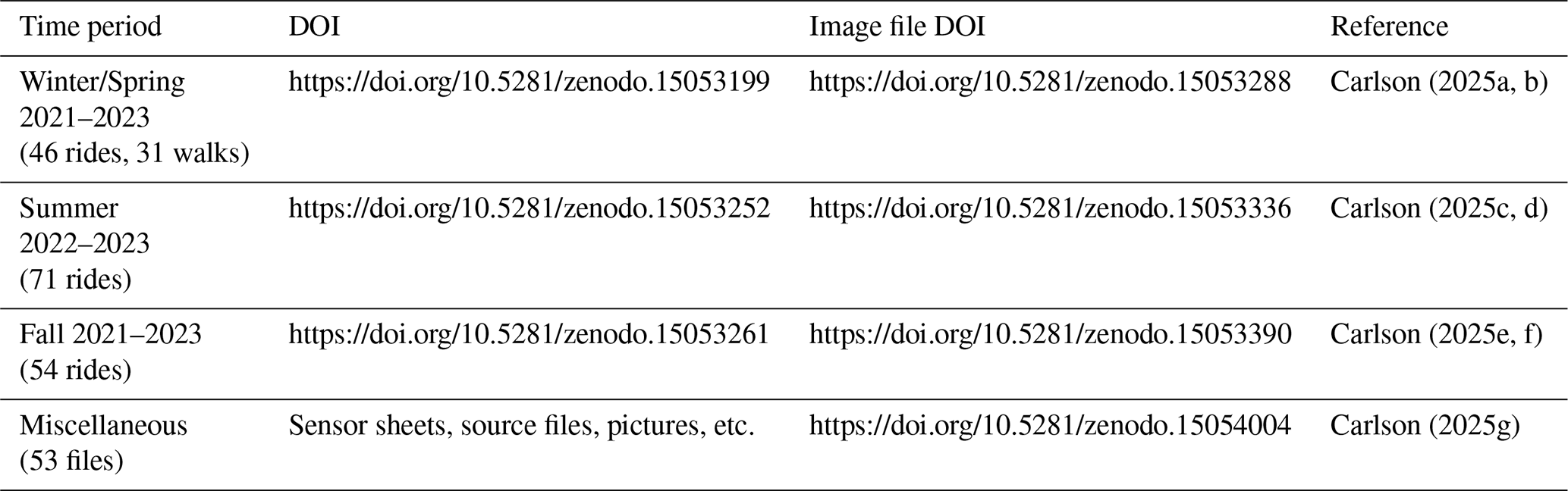
Table 2 lists all sources of data, images and miscellany.

Table 2 All data supporting this document, as stored on Zenodo, with urls, image files and references.

Each .csv data file carries date and ride location information in its title (“bike-20250228fowler”) with designations “fowler” and “bozeman” showing routes plus “north” or “south” indicating direction of Bozeman routes (south-bound if not otherwise indicated). Each .csv file (of ∼ 400 kb holding approximately 4000 records) carries detailed header information: GPS sec (UTC), longitude (degree.decimaldegree), latitude (degree.decimaldegree), TMP117 (°C) [in files after 18 November 2022], SHTC3 (°C), SHTC3 RH (%), Sfc IR (°C), IR board (°C), T_sfc-T_air (°C) [calculated], VEML6030 (lux), VEML6075 UVa (uW m⁻²), VEML6075 UVb (uW m⁻²), AS7263 A610 [absorbance], AS7263 A680 [absorbance], AS7263 A860 [absorbance], NDVI [calculated, see Appendix F]. Users can easily open .csv files in spreadsheets or GIS software or both. Please note: all analyses reported in this paper cover only September 2021 to October 2023 data, excluding recent (2025) data.

A second set of Zenodo files, listed in Table 2, holds sensor screenshots to demonstrate full data records for each ride: GPS heading (top panel); SHTC3, TMP (after 18 November 2022) and MLX90614 temperatures (second panel); T_sfc-T_air (calculated using SHTC3 air temperatures before 18 November 2022 and TMP temperatures after, third panel); then visible light (VEML6030) and NDVI (calculated from AS7263 wavelengths) overlain in fourth (bottom) panel. Horizontal axes nearly always cover one hour, demarcated at 6 min (∼ 500 data points) intervals. Vertical axes as labeled (heading directions, temperatures, temperature differences, light levels) include approximately consistent temperature ranges (e.g. around 25 to 30 °C) adjusted upward or downward primarily according to season, as necessary for convenient display. NDVI ranges (sometimes not shown) always cover 1.0 to −1.0. These images represent all-ride composites of data displayed in Figs. 7, 8 or 9. Users can easily peruse .png images to: (a) visually sort within or among Fowler loops vs Bozeman routes; (b) easily identify graveled stretches; (c) begin to recognize time of day or intensity of sunlight by direction, length and sharpness of shadows; then (d) choose a data file or files for subsequent spreadsheet analysis or GIS comparisons.

I also uploaded accessory data into a Zenodo folder entitled “Files to support bicycle data”. This folder holds bicycle and shading images, sensor data sheets and external data from local PV panels and from nearby NWS station. Users will find additional details in Appendix B. At https://doi.org/10.5281/zenodo.15054004 (Carlson, 2025g), users will find:

• Four tree-shading images, all .png and all as QGIS image exports using Google Earth backgrounds; these time-labeled images occur in Fig. 18 and Appendix E.

• Seven .jpgs, of bike, bike boxes and snow- or ice-covered road surfaces. Users will have seen all or portions of these images in Figs. 1 and 2 or used in Appendix G.

• One file – “Bike data from Google sheet” – representing a full data export, in .csv format, from the Google sheet that I used to track all rides and data files. This file contains standard columns for date, time, location, air temperatures, maximum surface temperatures, maximum light levels plus columns containing brief ride notes (“windy”, “body shading”, “rain”). Users might, for example, choose to compare notes on direction-dependent periods of body shading with actual light data. This particular .csv file contains valid entries for all 202 bicycle rides; read details in Appendix B.

• One file – “NOAA NWS-Gallatin” – with USA NWS “official” climate data (as displayed and explained in Fig. 10). I include these data in the event users encounter difficulty accessing NOAA's NCEI data repository.

• Three files recording daily power data from local solar panels (referred to in Fig. 11 and in Appendix C, all with relevant dates) plus one short (four-hour) record of photovoltaic power covering CW then CCW bicycle rides along Fowler loop on 30 June 2022.

• Nine files, all as .pdf, representing data sheets for all sensors described here:

  • –

    U-blox ZED9FP GPS unit;

  • –

    SHTC3 temperature and humidity sensor;

  • –

    TMP 117 temperature sensor;

  • –

    MLX90614 IR remote temperature sensor;

  • –

    VEML6030 visible light sensor;

  • –

    VEML6075 UV light sensor;

  • –

    MS8607 pressure, temperature and humidity sensor (deployed only on local roof);

  • –

    AS7263 wavelength-resolved near-IR sensor; and

  • –

    FS3000 air velocity sensor.

As described above, I do not provide bicycle-mounted Garmin 830 files for reasons of: (a) lower temporal and spatial resolution than u-blox GPS data; and (b) nearly-perfect redundancy of Garmin 830 data with u-blox GPS data (e.g. Fig. 3a). I keep the entire GPS 830 set, identified for times and routes, available to users on request.

I have also not included FS3000 air flow sensor data. That sensor ensured airflow across shielded temperature sensors. However, extrapolation of bicycle-based airflow data to, for example, road-level wind involves documenting exact instantaneous bicycle speed and direction, recording mean synoptic-scale wind fields plus known variations in space, time, and elevation, noting wind-sheltering effects of road-side trees, etc. Interested users can request FS3000 data.

8 Conclusions

Data described and available here come from a low-cost highly-reliable sensor package carried on a standard bicycle, deployed on roads and paths of semi-rural settings during all seasons in southwest Montana. Sharing this data proves utility and reliability of easily-available sensors carried on standard bicycles across typical paths and roads. It offers, for evaluation and use, open-access data comparing heating of impervious to pervious surfaces exposed to full sun or to tree-induced shade across snow-free and snow-covered seasons. At this moment, resolutions achieved by bicycle (4 to 5 m) exceed resolutions of freely-available satellite data (e.g. Landsat at 30 m, Sentinel-2 at 10 m); one anticipates convergence in the future with bicycle-based measurements supplying “ground-truth”.

These openly-shared bicycle-based data will prove useful to pavement engineers as well as climate researchers. The data cover important textural and insolation differences across roads and paths near Bozeman Montana. These data do not support models of heat island effects; they provide necessary baselines while stimulating researchers to identify missing factors. Citizens will emulate and extend these measurements.

Appendix A: Description of bicycle and its operation

I collected these data using a sensor box attached to front rack of a Surly Big Easy bicycle (Fig. A1), Despite occasional removals of sensor box for cleaning or upgrade (particularly after mishap on 18 November 2022), location, height, orientation and power (tapped from a USB port on the battery-powered handlebar-mounted light, Fig. A1) remained constant for all deployments. The bicycle itself provided steady speeds (via electric assist) and good traction (due to large tires) over many surfaces including gravel and snow.

I recorded times and positions from a bar-mounted Garmin cyclometer and independently from a controllable GPS in the sensor box (shown in Figs. A1, 1 and 2). Except when rider forgot to initiate bike-mounted Garmin, GPS records coincided perfectly in location while providing very accurate time synchronization (e.g. panel (b) of Fig. 2). Most rides started with intersection-wide loops to assess direction- or speed-dependence of sensor biases (see for example first or last seconds of nearly any record). Figure 2c shows an example of sensor box (higher time resolution) and Garmin unit (lower time resolution) GPS data during a standard start/end loop; I forced the sensor box GPS to record at 1.5 Hz while Garmin applied a proprietary recording interval. Although sensor data screenshot records include headings easily extracted from GPS data, Garmin data proved redundant to, and at lower spatial resolution than, independent self-recorded GPS-based time and location data from the bicycle-based sensor box (e.g. Fig. 2b). Users can request Garmin 830 data as supplements to u-blox GPS data.

Data collection on Fowler loop rides (∼ 15 km) covered approximately 45 min; northbound (“to”) Bozeman rides (∼ 10–12 km) covered ∼ 30–35 min; southbound (“from”) Bozeman rides (∼ 12–15 km) covered ∼ 55 min. Differences relate to specific routes and to descents northbound vs ascents southbound. For Fowler loops, average conditions over 110 rides indicated an average speed of 20 km h⁻¹. Twenty km h⁻¹ equates to ground speed of 5.6 m s⁻¹, suggesting effective spatial resolutions of approximately 4–5 m. A variety of wind, surface, and traffic conditions accelerated or delayed bicycle progress and thereby inflicted modest changes to effective spatial resolution; a “safe” conclusion indicated 4 m as probable along-track spatial resolution considering this bicycle, this rider and this sensor unit under these cycling conditions. Every data record included GPS-based timestamps and positions; users can determine specific spatial resolutions and locations of individual sensor data.

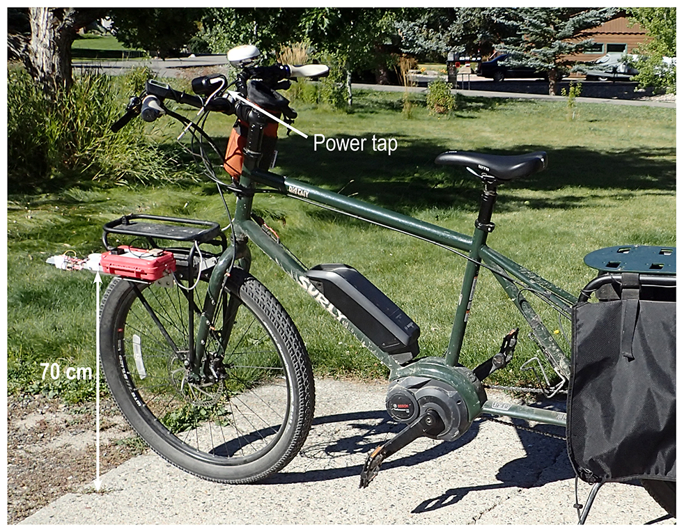
Figure A1 Surly Big Easy electric-assist bicycle with sensor package mounted on front rack. A fully-charged battery supported 80–90 km of lowest level (“Eco” mode) assist. In general, rides northbound involved slight descents, requiring little or no battery assist. Rides southbound typically involved slight ascent generally at second-level (“Tour”) assist. I never exhausted battery assist capacities. Sensors sat 70 cm above ground surfaces. Sensor box derived power from USB tap on rear of headlight.

Appendix B: “Complete” table of ride notes and summaries

This file, carrying the title “Bike data from Google sheet” in the Zenodo folder “Files to support bicycle data” (https://doi.org/10.5281/zenodo.15054004, Carlson, 2025g), provides a recent (March 2025) export (as .csv) from master data sheet maintained on Google drive covering summary data and notes for all rides. Column headers for this file include: Date, Start time (UTC seconds), Start time (local hour/minute), Route Distance (km), Ride notes (“windy”, “dusty”, “shaded”, “wet”, etc.), East/West air temp (C), South 3rd air temp (C), Sfc-air mean (C), Sfc-air min (C), Sfc-air max (C), lux (min), lux (max). In personal version (not shared) I might also track processing steps, correlation values, color code rows by season, etc. “East/West” air temperatures refer to data measured during west-bound travel along Bristol Lane at the start of Fowler loops; these data might hold useful insights not explored here. I share this minimal version so that users can reproduce e.g. Figs. 10 or 17. Users might also want to know local times, maximum light (lux) values, etc.

Appendix C: Visible and UV light comparisons and “validations”

These particular data (Figs. C1 and C2) supplement data presented in Fig. 11, albeit for other seasons. Due to fewer data, I have not produced a plot for December–January–February.

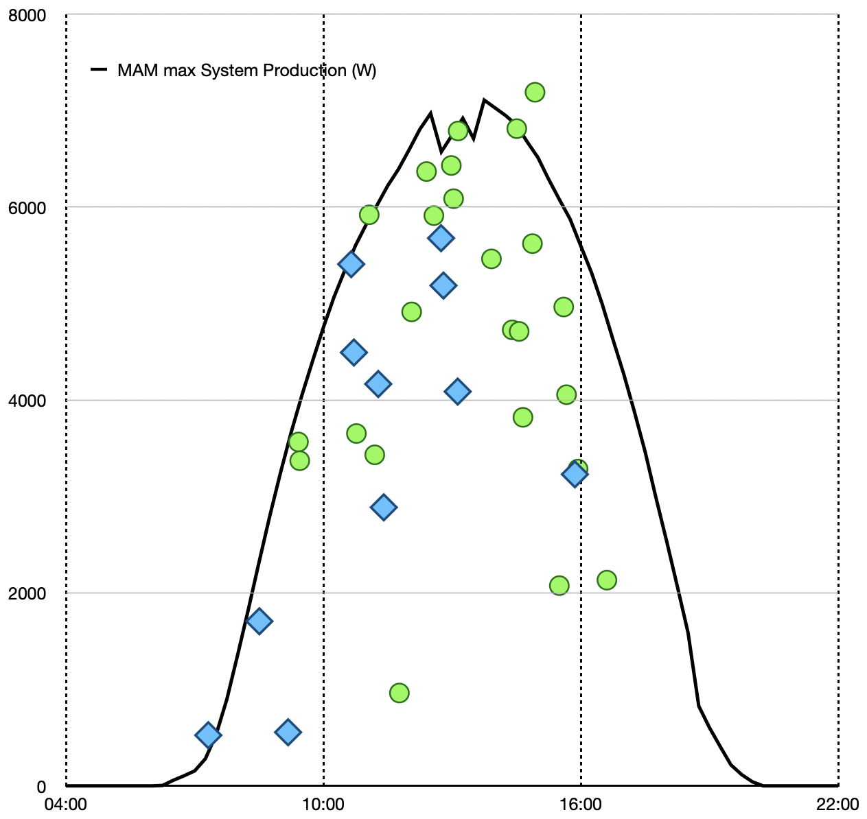
Figure C1 Exactly as in Fig. 12, but for March–April–May (MAM): maximum illumination values from bicycle-mounted VEML 6030 sensor sorted by start times for bike rides around Fowler loop (green dots) or to-from Bozeman (blue diamonds), compared to maximum power records from roof-mounted photovoltaic panels, for all MAM ride data from 2022 and 2023. Photovoltaic data, recorded as 15 min power output summaries (solid black line), came from 1 May 2023. Bicycle data represent maximum illumination data, in lux, measured during full MAM rides, e.g., not restricted to oft-ridden stretch of pavement on south 3rd Avenue. Data gathered from shaded or graveled stretches of pavement should have no impact on insolation maxima.

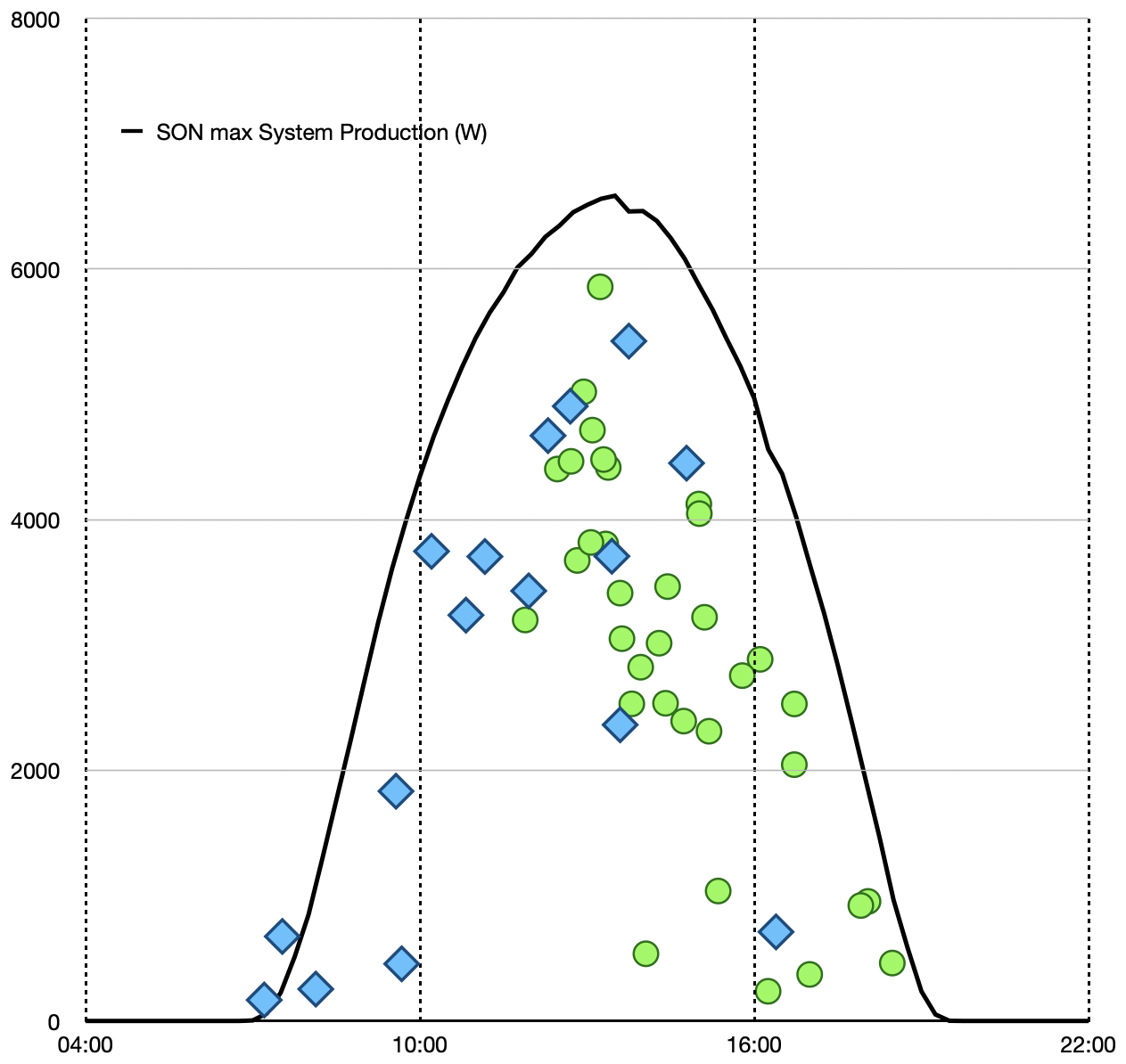
Figure C2 Exactly as in Figs. 12 and B1, but for September–October–November (SON): maximum illumination values from bicycle-mounted VEML 6030 sensor sorted by start times for bike rides around Fowler loop (green dots) or to-from Bozeman (blue diamonds), compared to maximum power records from roof-mounted photovoltaic panels, for all SON ride data from 2021 to 2023. Photovoltaic data, recorded as 15 min power output summaries (solid black line), came from 10 September 2023. Bicycle data represent maximum illumination data, in lux, measured during full SON rides, e.g., not restricted to oft-ridden stretch of pavement on south 3rd Avenue. Data gathered from shaded or graveled stretches of pavement should have no impact on insolation maxima.

Appendix D: Graveled surfaces

Figure D1 demonstrates, using Fowler data from 7 June 2023 (users can monitor this discussion by looking at sensor data image from 7 June 2023), persistently cooler properties of graveled surfaces. One assumes that persistently cooler surface temperatures for pervious (graveled) road or path surfaces versus impervious (paved) road surfaces relate to absence of asphalt binders (see Introduction and Sect. 5.4). Instances of tree shading coupled with color-than-impervious graveled surfaces occur frequently. As Fig. D1 demonstrates, graveled surfaces often showed temperatures at least 5 °C cooler than adjacent impervious surfaces, and contained distinctly cooler regions due to tree-induced shade. Some graveled areas proved ≥ 7 °C cooler than adjacent impervious surfaces; other rides on other days produced gravel temperatures cooler than adjacent impervious surfaces by 10 °C. Cooler surface temperatures of graveled surfaces proved pervasive throughout these bicycle-gathered data, albeit never with corresponding diminutions of overlying air temperatures.

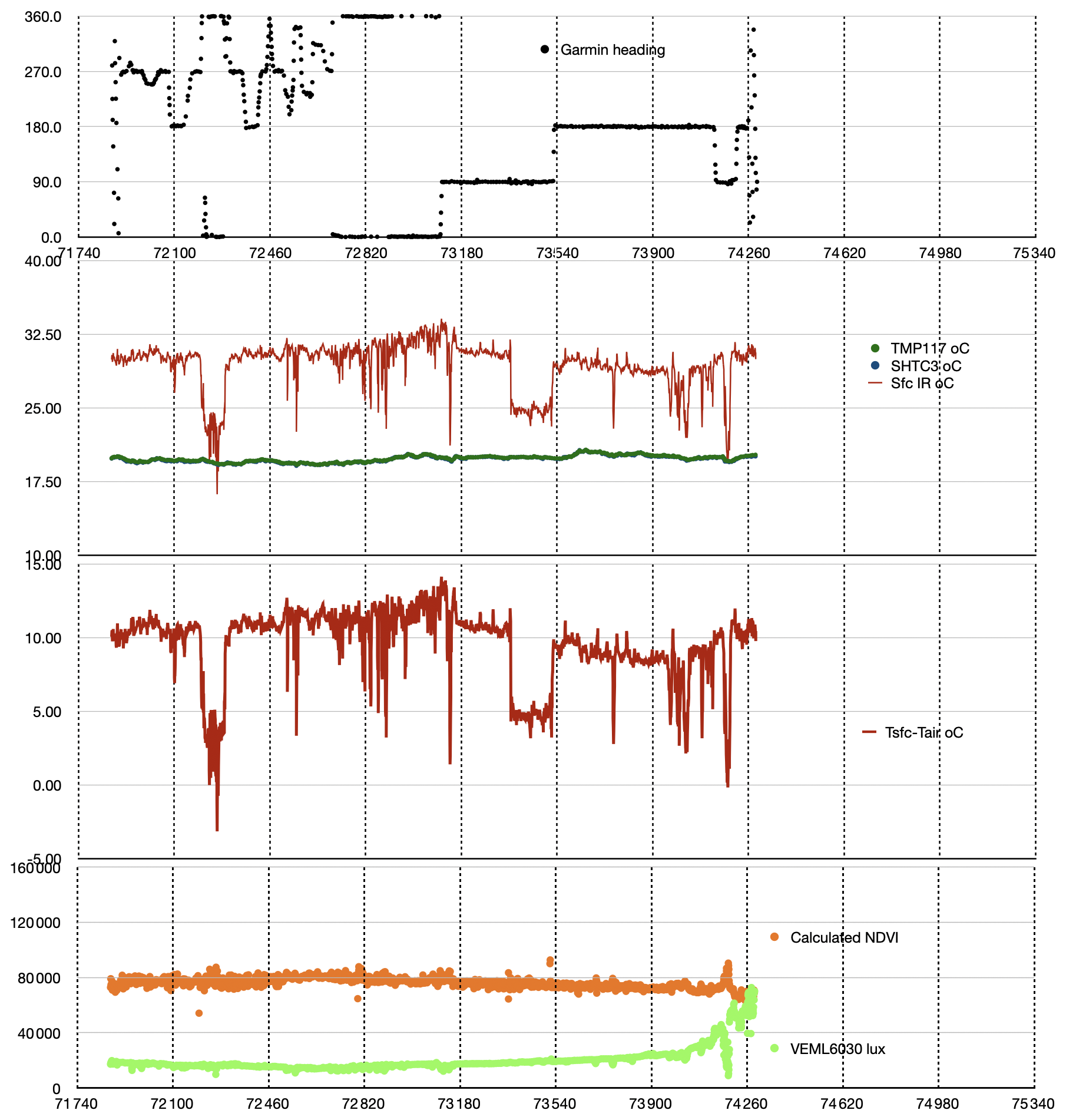
Figure D1 Data from Fowler loop ride on 7 June 2023, demonstrating cool surface temperatures on south-to-north (around 72 200) and west-to-east (starting from ∼ 73 350) graveled (pervious) surfaces compared to adjacent impervious (paved) surfaces. As generally occurred across full data set, on this particular very-cloudy ride sensors recorded cooler gravel stretches independent of changes in air temperatures or insolation. Top panel: GPS headings. Second panel: surface (red lines) and air temperatures (blue dots from TMP117 and green dots from SHTC3, indistinguishable at these scales) plotted together over temperature range of +10 to +40 °C. Third panel: T_sfc-T_air (red lines) plotted over temperature difference range of −5 to +15 °C. Bottom panel: light data (green dots from VEML6030) plus calculated NDVI (orange dots, using wavelengths of 680 and 860 nm from AS7263). Time (along horizontal access) runs from 71 740 to 75 340 GPS seconds, 3600 total seconds, 360 s (6 min) per grid line. Ride took 42 min to cover 15.06 km, starting from 13:56 local time.

Appendix E: Shading impacts

In small regions, for example ∼ 100 m stretches at NW corner and SW ditch/creek crossing of Fowler loop and frequent short stretches of Bozeman rides particularly along pedestrian paths, tree coverage and consequent persistent shade provided cooler surface conditions than adjacent full-sun regions. Close inspections of Fig. 1 clearly demonstrate shaded regions of Fowler and Bozeman routes, as do temperature-time plots of Fig. 12 and spatial data of Fig. 14. These data show that persistent shade leads to persistent surface cooling (including in winter) but that, in absence of shading or due to changes in exposure that result in removal of shade, surface temperatures quickly revert to “normal” for that ride at that time of day.

Intermittent shading, as from a road-side tree at early or late sun angles, presents a stiffer challenge but one still easily resolved in these data. Figure 18 demonstrates CW (standard) followed by – minutes later – CCW Fowler loop rides: the impact of one set of road-side trees shows very clearly on the first southbound pass along the west lane but has no impact a few minutes later as I rode back along the eastern lane. Both rides occurred around 15:00 local time. (The Google Earth image, conveying roughly the same sun angle, tends to reinforce measurements).

Figure E1a–c demonstrate similar data gathered a few weeks later (27 July 2022) on a northbound Bozeman ride followed (roughly two hours later) by a southbound return ride. Panel (a) shows the identical spot presented in Fig. 18: west-side trees along south 3rd. In this early case (07:00 start, 09:00 return) neither initial northbound nor later southbound rides showed any shading impact by west-side trees. Panel (b) shows exit from (northbound) then return entry onto (southbound) one of Bozeman's much-used pedestrian paths. Later southbound image demonstrated stronger surface heating in sun-exposed areas plus stronger surface cooling in tree shaded areas: more-intense solar insolation provoked both more heating and sharper shading/cooling. Panel (c) demonstrates a similar effect. Sensors in early northbound passage showed modest to slight impacts of exposure or shading while same sensors recorded, during later southbound passage, stronger surface heating in exposed areas and stronger surface cooling in shaded areas.

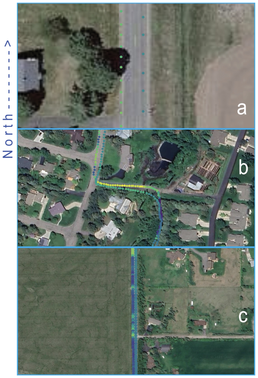
Figure E1 Data from a northbound (07:00 local time) Bozeman ride followed by a southbound return ride a few hours later (after 09:00 local time), using identical temperature scales northbound and southbound, both on morning of 27 July 2022. (a) Data from early northbound ride (right track in east lane) followed less than 3 h later by return (09:30 local time) southbound ride (left track in west lane). Identical location as in Fig. 19. At these hours, with solar illumination from the east, neither ride shows any shade impact of trees on western roadside. (Google Earth image from Fig. 19, used again as background, recorded under late day conditions tends to confuse this early-in-the-day pattern). (b) Same day, same routes, showing data from northbound track (slightly mis-aligned) then southbound return track as I crossed from (rode into) pervious shaded graveled path via short paved (impermeable) access onto (from) standard Bozeman city streets. In this figure, later ride shows both sharper surface warming in sun-exposed spots and sharper surface cooling in tree shadows; rising morning sun tends to heat exposed surfaces while trees shade cooler surfaces. (c) Same day, same routes, showing data from south 3rd, along eastern tree-lined stretch. Early northbound (07:00) track (right track along east lane) shows minor distinctions between shaded and un-shaded stretches. Later southbound return trip (left track along west lane) shows more surface heating in exposed areas plus stronger surface cooling in shaded stretches. Analysis from QGIS; background maps from © Google Earth.

Appendix F: Light measurements and NDVI calculations

Intercomparisons of light data involve wavelengths, energy, exposures, units, etc.; not an easy task in “fixed location cases”, perhaps more difficult if one wants to validate systems involving sensors moving between full sun and deep shade. Here I evaluate three insolation components: a VEML6030 sensor on a bicycle, an identical VEML6030 sensor mounted next to and parallel to roof panels, and roof-mounted photovoltaic panels measuring photovoltaic power in watts. Figure 6 proves excellent correlations between roof-top panels and an adjacent roof-top VEML6030 (the former recording power generation data in watts every 15 min while the latter records insolation in lux from 10 measurements averaged and transmitted every 5 min). Clouds should impose similar impacts on roof-top panels and roof-top light sensor, at least over longer (hourly, diel) time spans. Figures 11, C1 and C2 prove efficacy of comparing time-resolved bicycle light maxima to daily power-based insolation patterns; those intercomparisons prove effective and appropriate. Because of visible differences in terrain and cloud cover, however, I did not compare local light (from photovoltaic panels or from roof-top VEML6030 sensors) to 25 km distant NWS-generated light data. What about VEML6030 sensors on a bicycle, gathering data at faster than 1 Hz? With bicycle rides, at least for Fowler loop, complete within ∼ 45 min, one might get at most four data points from photovoltaic panels reporting every 15 min; not useful to extrapolate from ∼ 4000 bicycle data points to 4 roof-panel data points. Roof-mounted VEML6030 sensors, recording over ∼ 30 s while reporting at five minutes repeat frequency, offered useful validation bridge even as bicycle sensors moved in and out of local shade or experienced (during a ride) changes in cloud cover. Users will develop confidence in comparisons of like-for-like sensors (e.g. Figs. 6, 11, C1 and C2 compared to any seasonally-appropriate sensor data image). Users will also quickly learn to identify and trust light changes, seasonal and direction-dependent rider shading (generally recorded in ride notes), and differing visible, UV and near-IR patterns related to rider-shading versus, for example, clouds. An overall nested combination of slower power-based photovoltaic data with faster VEML6030-based adjacent roof-top data then with very fast (> 1 Hz) bicycle data can prove useful!

Pavement albedo (ratio of incoming to reflected light) might represent a determining factor in other environments (e.g. Pomerantz et al., 2000) but sensors used here provided unique valid records of both insolation and surface heating. Users can, if desired, calculate albedos by assuming spectral shapes normalized to AS7263 “red” data, but actual measurements prove that, for these environments under these measurement conditions, air temperatures did not respond to underlying surface warming or cooling. Albedo changes, modest in any case, proved irrelevant? Even under maximum surface heating conditions encountered within large cities, maximal plausible changes in albedo played only small (< 0.6 °C) roles in surface-driven heat effects (Pomerantz et al., 2000); their observations neither explain nor contradict these measurements. Does solar insolation warm surfaces? Yes, definitively (see Fig. 17), but other factors also pertain (data spread in Fig. 17). Should users therefore assume durable heat island influences? Not from these data as presented. We require more-careful, more-thorough assessments to account for urban heating effects.

This configuration of sensors on this particular bicycle did not result in ideal locations for visible (VEML6030, see Figs. A1 and 2) or UV light sensors (VEML6075, again Figs. A1 and 2). Rarely at some seasons and times of day, upward-looking light sensors fell into shade of rider's body or of bicycle handlebars or cables. These shaded directions and periods (often recorded in notes accompanying each ride, see Appendix B) emerged distinctly in recorded light (Vis and UV) data (see for example Fig. F1).

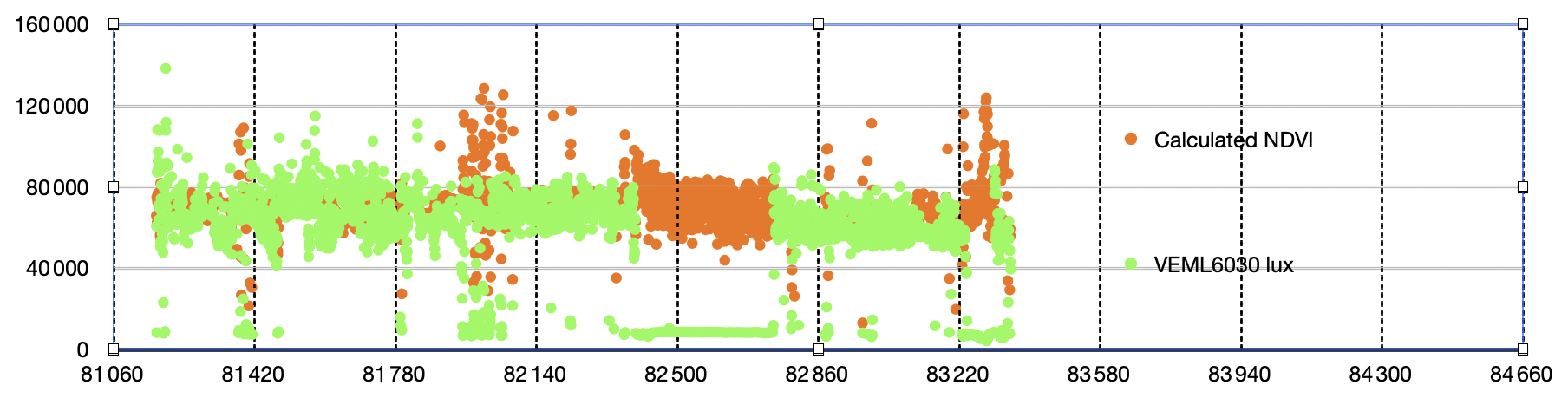
Figure F1 Data from Fowle loop ride on 9 August 2022, demonstrating cyclist-induced shading of light sensors on eastbound legs. Light data (VEML6030, green dots) plus calculated NDVI (orange dots). VEML6030 data show sharp distinct diminutions (to very low lux) during two eastbound stretches starting around 82 400 and 83 200 s (approximately 17:00 and 17:10 local times). Light levels measured by VEML6030 remained approximately 60 000 lux before and after periods of cyclist shading.

Moments or stretches of rider-induced shading of light sensors, easily distinguished from tree-induced or cloud-induced shading (clouds induce a more gradual transition with “softer” edges), did not affect air or surface temperatures. For replication of rider-shading of light sensors, users can look at starting or ending loops (for example, in Fig. F2). There users will often note distinct directional influences on VEML6030 data, recorded accurately as bike changes of direction. Note also (e.g. in Fig. 15) absence of corresponding direction or speed-dependent impacts on surface or air temperatures.

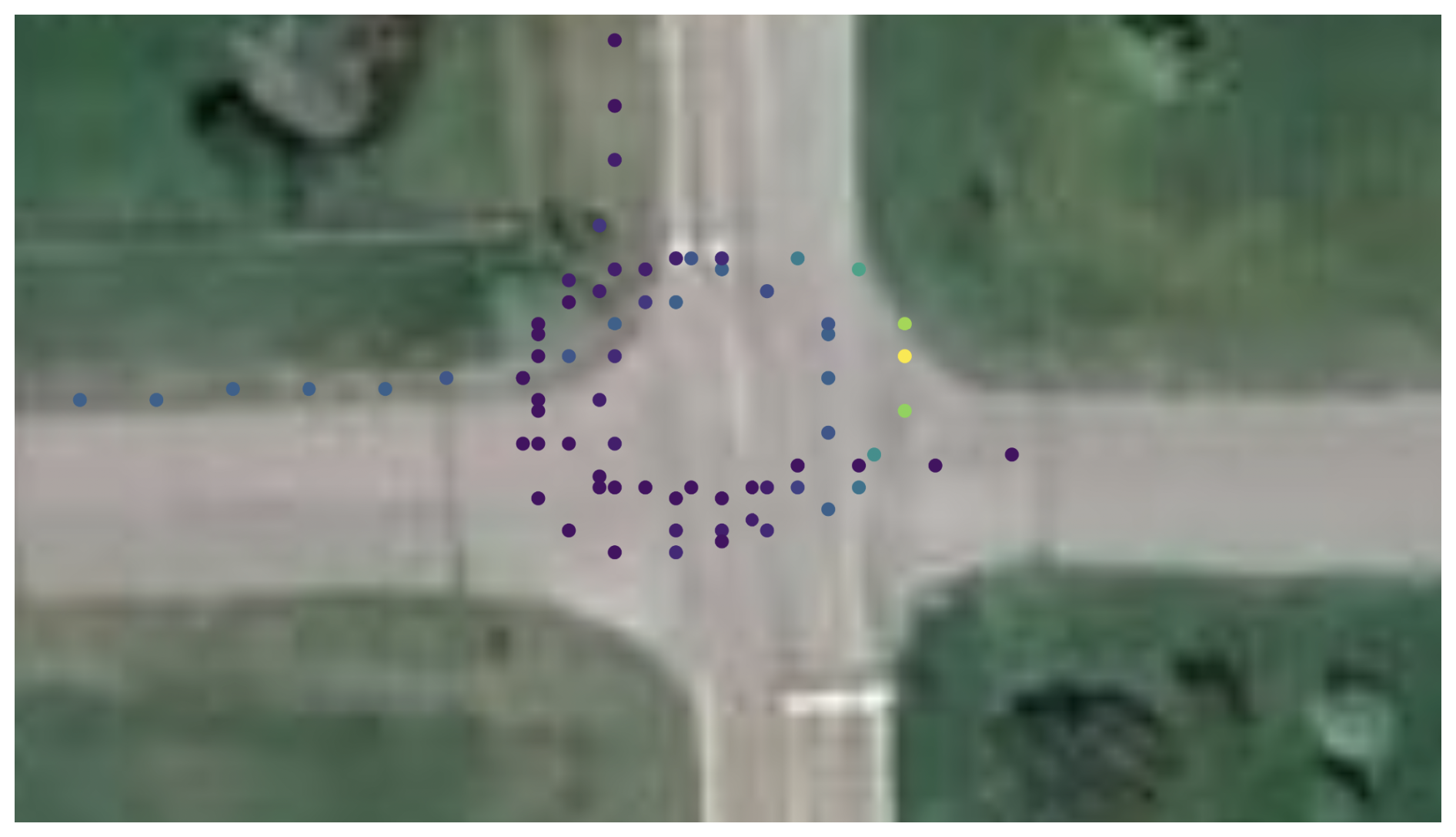
Figure F2 Data from Fowler loop ride on 4 October 2022, demonstrating cyclist-induced shading of light sensors during start and end loops. This image displays same tracks as in Fig. 15 (albeit with Google Earth background) but with VEML6030 lux data. For both start and end loops, light data showed greater values in northbound directions (upper right part of image) than in eastbound (lower left) directions. Background data from © Google Earth.

NDVI producers or users will know standard ranges of NDVI products: +1.0 to −1.0. NDVI calculations used here came from ratios of 680 and 860 nm data from AS7263, according to widely-accepted formula: 860–680 nm/sum of 680 nm plus 860 nm. This author does not propose to open voluminous NDVI literature and interpretations. I want to offer, based on characterizations of surfaces and temperatures of those surfaces, the possibility of applying local high-resolution but inexpensive data to larger NDVI applications and of interpreting satellite-based NDVI records based on bicycle-based surface data.

Appendix G: Winter conditions on impervious surfaces

Figure G1 demonstrates the considerable range of snow and ice coverage of impervious surfaces available in this data set. Each of these conditions (packed snow versus vehicle-tracked ice) imposed different thermal and visible signatures.

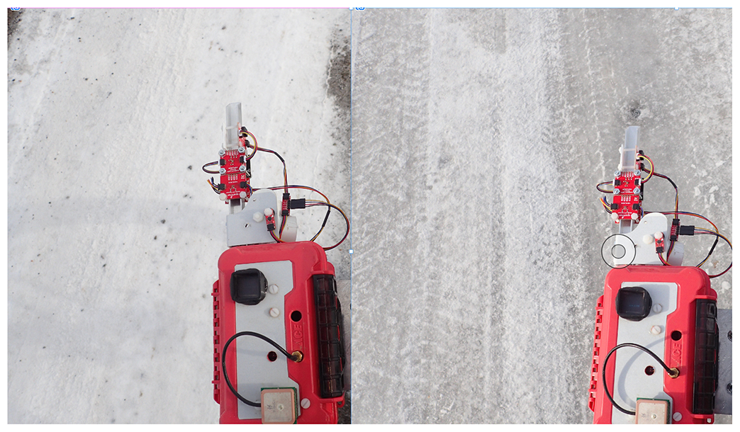
Figure G1 Data from Jade walk on 9 March 2023. Left image shows typical packed snow surfaces, after modest snow plowing. Right image shows vehicle-packed ice, with vehicle wheel tracks clearly visible.

Figure G2 demonstrates (imperfectly) how pavement temperatures differ between bare (end of cleared drive in near view), snow-covered, and (in the distance) bare surfaces. Pavement surface temperature differences from air temperatures varied in this case from near 0 °C (air temperatures remained steady at +5 °C throughout this record) over near-view snow to +10 °C over cleared drive to greater than 10 °C on solar-warmed pavements. A demonstration video (https://youtu.be/nMjBFbXxNWU, Carlson, 2025h) combines drone plus bicycle-based videos with overlaid T_sfc and T_air data to provide users a better sense of extensive snow cover interspersed with spots of cleared or melted pavements, plus clear impacts of shade.

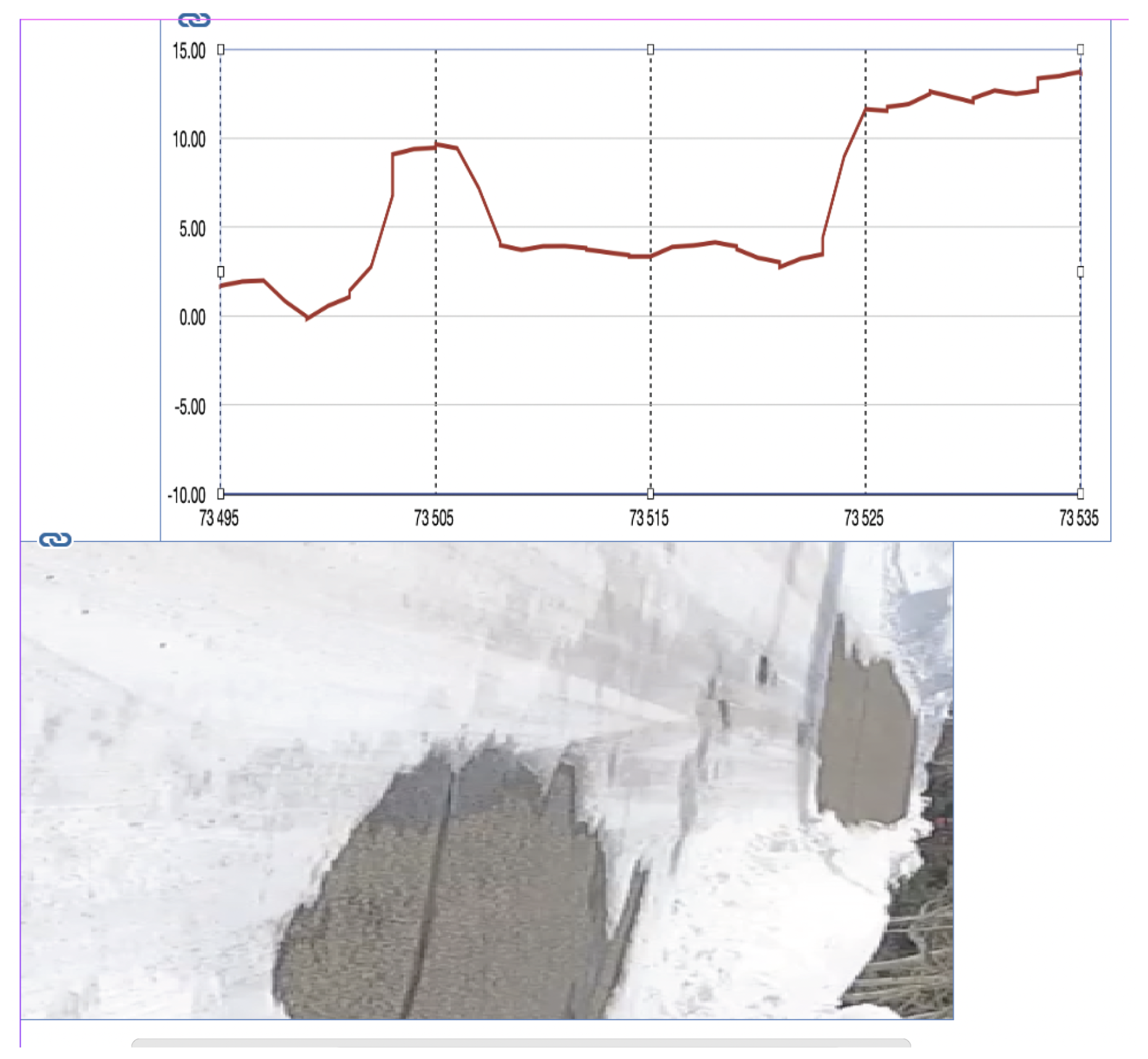
Figure G2 Surface temperatures (top panel) superimposed over static photo of snow then shaded snow followed by bare (end-of-drive) surfaces, followed again by ice-covered then shaded then bare surfaces. Surface temperatures clearly respond to changes in surface coverage. Demonstration video shows this case in much better detail.

Appendix H: Durability of these sensors

A bicycle ride on 28 February 2025, 16 months after “final” (October 2023) data described here, proves long term durability of these sensors. I used same bike, same box, same sensors, and same power, on a ride to and from north Bozeman; I recorded this data under appropriate file label (28 February 2025 Bozeman) but never included 2025 data in any analysis above. These data reveal interesting features, ripe for confirmation or refutation by subsequent bicycle riders.

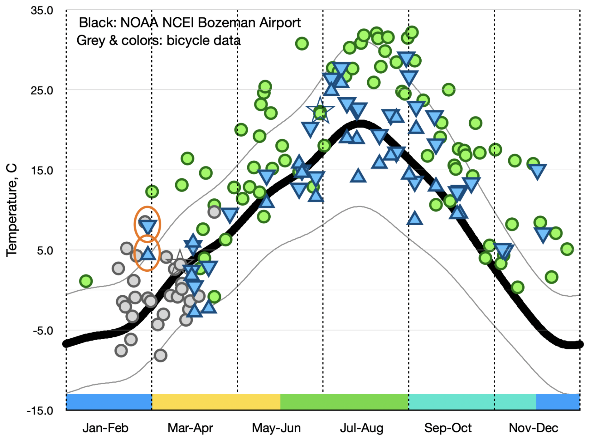
Figure H1 Data exactly as in Fig. 11 (above) with additions (circled in orange) of northbound (upward triangle) and southbound (downward triangle) data from 28 February 2025. Within normal variations due to weather, sunlight, etc., 2025 data fit perfectly with all prior data.