Thermo-hydrological river valley observatory in Yedoma permafrost from 2012 through 2022 in Syrdakh, Central Yakutia

Permafrost thaw affects the global carbon cycle and can significantly alter landscape morphology and associated processes of mass and energy transfer. An understudied aspect of thaw-affected permafrost landscapes is ubiquitous rivers connecting thermokarst lakes. These features of Arctic landscapes exhibit particularly high variability in water and energy transfer because, in lakes with larger water storage, excess water leads to comparatively small changes in water level and discharge, whereas in streams the channeled flow produces much larger fluctuations. Consequently, an equivalent absolute change in water level represents a much smaller relative change in lakes than in streams, resulting in a comparatively minor impact on overall heat content and energy transport. Such rivers thus provide an excellent field laboratory for analyzing how expected changes in meteorological forcing under climate change affect permafrost dynamics and carbon exchange within the land- and limnoscape. This paper presents a database from 2012 through 2022 for one such small stream connecting two thermokarst lakes. We instrumented two main stream cross sections with multiple subsurface thermistor chains to record temperature evolution from the land or water-land interface (≥ 5 cm depth) to soil depths of up to 5 m. The cross sections covered different topography and vegetation cover. One was located near the upper, and one in between the two thermokarst lakes. The main focus was set on the cross section midway between the two lakes (CS 9) due to the absence of a thermal imprint from the lake. Air, water, and ground temperatures, as well as physio-chemical river water and soil properties of the surrounding environment were measured continuously or during annual field campaigns and are provided as time-series or single tests. The data are organized in three main categories: atmosphere, water and ground, and are complemented by a GIS database including a digital surface model and an ortho-mosaic photo of the entire river valley to facilitate the search for measurements of interest. The database comes with a complete set of scripts to process any of the data, which are provided in CSV or other easily accessible standard file formats. Ultimately, the data can be used to develop models and validate numerical codes for improving the representation of permafrost processes in land surface and climate models where climate change induces significant changes in heat and mass transfer. All data and processing scripts are available through an online repository (https://doi.org/10.5281/zenodo.14619854, Pohl et al., 2025).

1 Introduction

Recent increases in air temperature in the Arctic and sub-Arctic regions have been well above global average trends (Meredith et al., 2019). Consequently, permafrost in these regions has experienced significant warming (Biskaborn et al., 2019; Melnikov et al., 2022). Thawing of ice-rich permafrost affects a multitude of geomorphological and biogeochemical processes. Landscape changes by means of ground subsidence, mass movements, and ground stability affect infrastructure (Hjort et al., 2022) and hydrology (Walvoord and Kurylyk, 2016); increased hydrological connectivity and activation of organic matter activate formerly inactive biogeochemical cycles (Miner et al., 2021, 2022). One specific feature of thawing ice-rich permafrost is the formation of thermokarst lakes (French, 2017), which are impoundments of water in the resulting depressions with positive feedback between lake growth and permafrost thaw (Grosse et al., 2013). These lakes and their connecting streams alternate the dominant heat transfer processes and drive a climate feedback cycle including the activation and mobilization of large carbon stocks (Hugelius et al., 2014; Mishra et al., 2021; Miner et al., 2022) with global socio-economic impacts (Hope and Schaefer, 2016; Schuur et al., 2015).

The ground thermal state of permafrost can show high spatial variability. Sparse observation networks for air, and particularly for soil and deeper ground temperatures (e.g. Boike et al., 2019), as well as a large range of processes involved in the modes of heat and water transfer render past and future predictions of permafrost evolution difficult (Koven et al., 2013). Additionally, a multitude of important small scale processes related to heat and water fluxes in permafrost landscapes (Walvoord and Kurylyk, 2016; Westermann et al., 2016, 2017; Aas et al., 2019; Song et al., 2020; Steinert et al., 2021; Tananaev and Lotsari, 2022) are barely represented in regional to global scale land surface and climate models operating at coarse spatial scales. This is despite the need for such models to produce reliable estimates of ground-atmosphere interactions and represent the interactions and feedback that a warming climate has with permafrost landscapes. Improving small scale process representations and how these can be accounted for at larger scale is therefore of high importance (Grenier et al., 2018; Jan et al., 2020).

One particular emerging landscape feature that has received rather limited attention is small rivers and creeks that connect or drain newly developing thermokarst lakes (e.g. Liu et al., 2022; Tananaev and Lotsari, 2022). In general, Arctic rivers are characterized by high seasonal flow variability (e.g. Gautier et al., 2018) inducing a likewise high variability in heat transport at the water-land interface, subsurface saturation and flow, and as a consequence, also in solute and particle fluxes. Compared to perennially unfrozen water bodies of lakes and large rivers, where ice thicknesses might reach a maximum of 1.5 to 2 m (Lütjen et al., 2024), small rivers and creeks might experience freeze-through. Here, the water bodies do not provide heat to maintain a talik (an unfrozen zone underneath the river or lake bed that can form for large enough water bodies, Kurylyk and Walvoord, 2021; Léger et al., 2023).

A warming climate implies the formation of more water bodies, in particular small rivers connecting newly formed thermokarst lakes (e.g. Morgenstern et al., 2011; Tananaev and Lotsari, 2022). Continued observations, not only of the thermal state of permafrost but also of the multiple other types of variables required to understand the changes to permafrost, are therefore of great importance (e.g. Boike et al., 2019).

This paper presents a database of an observatory of a small non-perennial river or stream (namely the Syrdakh River) in the Syrdakh valley in Central Yakutia, Eastern Siberia (Pohl et al., 2025). This region is underlain by the Yedoma ice complex (30 to 50 m), defined as ice-rich, fine-grained permafrost deposits of late-Pleistocene age (about 70 %–80 % ice per volume), composed of frozen silts and silty sands penetrated by several meter-thick syngenetic ice wedges (Ivanov, 1984; Strauss et al., 2021). We assume our study site, therefore, is representative for large parts of the Yedoma permafrost domain (Strauss et al., 2021), prone to permafrost thaw and consequent landscape changes. The data aim particularly at serving the validation and calibration of numerical modeling code for heat and water transfer processes in the ground and at the water-ground interface. Therefore, monitoring of ground temperatures and the determination of physical ground parameters for relevant processes were the focus of the instrumentation and the annually performed tests. The two main observation sites in the form of cross sections are located between two large thermokarst lakes: one site about 50 m downstream of the “upper lake” with assumed thermal influence of the lake water body, and one site a few hundred meters away (further downstream) without such thermal influence.

2 Site description

The Syrdakh River (62.555 to 62.562° N, 130.900 to 130.961° E) is located about 100 km northeast of Yakutsk in Central Yakutia (Eastern Siberia), Russia (Fig. 1), within the continuous permafrost zone (300 m in thickness, Soloviev, 1973). The climate is sub-Arctic and strongly continental with long, cold and dry winters (January mean temperature ≈ −40 °C) as well as warm summers (July mean temperature ≈ +20 °C). This results in a notably strong seasonal variability, with annual extremes of nearly 100 °C between minimum (−60 °C) and maximum (+35 °C) temperatures (Gorokhov and Fedorov, 2018). Total precipitation is low (< 250 mm) and mostly confined to the summer, resulting in a relatively low winter snow cover (< 30 cm) (Gorokhov and Fedorov, 2018). The evapotranspiration rate is high, up to ten times the precipitation in summer during dry years (about 150–200 mm on average). The region is characterized by taiga vegetation dominated by larch, pine and birch forests with dense shrub cover in forested areas and steppe grasses or bog plant communities (salt-tolerant species) otherwise. Active layer thicknesses vary between ≈ 1 m below forested areas to > 2 m in exposed grassland areas (Yukechi, 61.75° N, 130.47° E) (Fedorov and Konstantinov, 2008; Fedorov et al., 2014); slightly higher values between 1.37 and 1.67 m are reported for a larch forest site near Yakutsk (Spasskaya-pad, 62.23° N, 129.62° E) (Iijima et al., 2010). Central Yakutia underwent a strong warming trend of ≈ +0.05 °C yr⁻¹ for the period 1966–2016 (Gorokhov and Fedorov, 2018; Fedorov et al., 2014). Numerous thermokarst lakes of different origin are observed in the region: early Holocene thermokarst led to the formation of thermokarst basins called alas (Soloviev, 1973), while during the early 1990s an intense thermokarst formation period created many small thermokarst lakes (Fedorov and Konstantinov, 2008; Iijima et al., 2010).

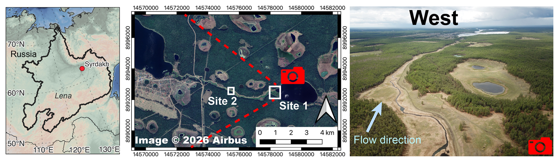
Figure 1 (A) General location of Syrdakh in Siberia within the Lena River catchment (black outline), (B) Google Earth imagery of the Syrdakh valley showcasing the alas lakes within the forested surrounding areas, and the two thermokarst lakes as well as the location of the two main sites (Site 1 and Site 2), (C) UAV aerial oblique view from the upper lake towards the lower lake showing the river and alas lakes. Coordinates in (B) are in WGS84 UTM zone 52N. Data source for (A) is the Earth Topography (ETOPO1) digital elevation model in 1 arcmin resolution (NOAA National Geophysical Data Center, 2009; Amante and Eakins, 2009). Data source for (B) is Google Earth (Image © 2026 Airbus; Google, 2026).

The presence of numerous small and young (< 50 years), fast-developing thermokarst lakes (> 3–4 m deep) and retrogressive thaw slumps along lake shores attest to the recent warming in the area (Morgenstern et al., 2011; Desyatkin et al., 2015; Séjourné et al., 2015). These younger thermokarst lakes are observable alongside older (early Holocene) and shallower (≈ 1 m deep) alas lakes.

The small non-perennial Syrdakh River connects two thermokarst lakes from east to west over a distance of around 3 km (Fig. 1). The river is located on a lowland plain between the Lena River to the west and the Aldan River to the east (Hughes-Allen et al., 2021). Its watershed size is approximately 440 km² with a total elevation difference of 30 m (Heberger, 2022; Yamazaki et al., 2017; Amatulli et al., 2018). The thermokarst lakes have surface areas of 0.61 and 1.75 km² for the upper and lower lake, respectively; water depths in the upper lake were determined in 2012 (with an echo sounder from an inflatable boat), reaching up to 6.4 m. Ice cover reached a thickness of 0.7 m during the winter 2018/2019 (Hughes-Allen et al., 2021).

In 2012, we installed the first thermistor chains at various depths, following a similar installation setup for ground temperature measurements elsewhere in Siberia by the Melnikov Permafrost Institute (MPI). Various depths, either using the common measurement depths by the Russian Federal Service for Hydrometeorology and Environmental Monitoring (Roshydromet) at 60, 120, 240, and 320 cm or at evenly spaced depths of 1, 2, 3, and 4 m were used. When it comes to using the data for numerical modeling, both setups have advantages and disadvantages; the latter provides more data at different depths (rather than a higher resolution at shallower depths). Over the following years, we extended these installations with soil measurements (e.g. granulometric soil composition, soil infiltration, thermal soil parameters), measurements on water chemistry (e.g. stable water isotopes, conductivity, pH), as well as geophysical measurements (e.g. Ground-Penetrating Radar (GPR), Electrical Resistivity Tomography (ERT)) at other cross-sections (Fig. 2). The installation of instruments was conducted at two main sites, one (Site 1) near the upstream thermokarst lake and one (Site 2) roughly half way between Site 1 and the downstream thermokarst lake, where the village of Syrdakh is located. Multiple instrument failures, particularly of instruments installed in the river and riverbed, have led to the discontinuation of instrument reinstallation and maintenance at Site 1. In addition, the focus of the database revolved around the thermal imprint of rivers. As a consequence, Site 2 became the prioritized site where most measurements were conducted. At Site 2, piezometer tubes were installed along a cross section (CS 9), with most of them positioned approximately 2 meters apart, in form of PVC tubes with 50 mm diameter. They were inserted into boreholes with a diameter of 66 mm that extended into the permafrost. These boreholes were made using a petrol-powered drill. In 2019, a new row of piezometer tubes was installed at CS 9 to modernize the tubes.

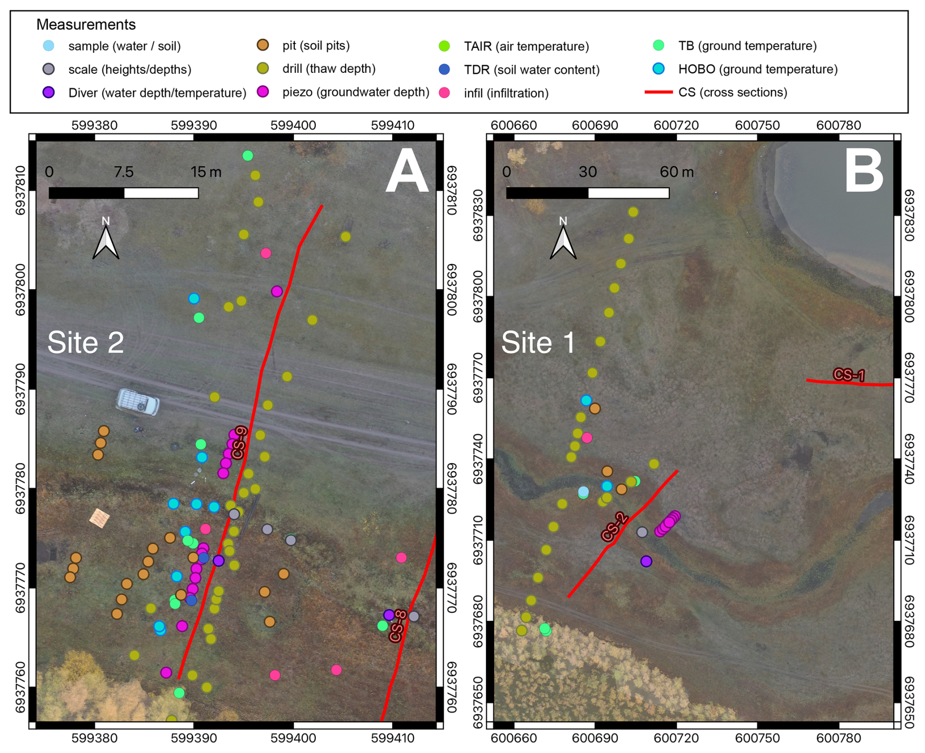
Figure 2 Zoomed in views of highly instrumented cross section CS-9 or “Site 2” (A) and CS-2 referred to as “Site 1” (B). Coordinates in the zoomed in views are in WGS84 UTM zone 52N.

3 Database

The database comprises files of different data and information types. All data are provided in non-proprietary file formats to achieve easy accessibility across platforms. All times are provided in UTC; the local time zone of Syrdakh is UTC + 9. All data files follow a naming convention outlined in Sect. 3.3. All variable names, relevant instruments and their characteristics, including accuracies, resolution, and measurement intervals, are listed in Table .

(Kachinsky, 1965)(Synal et al., 2007)

Table 1 List of variables, sensor or instrument names, type of measurement (time-series $<x>$ ts, tests $<x>$ test, for atmosphere (x=A), water (x=W), and ground (x=G)), and instrument characteristics. Multiple measuring intervals reflect changes in the instrument configuration over the years and that some measurements are obtained through annually conducted tests (1 year).

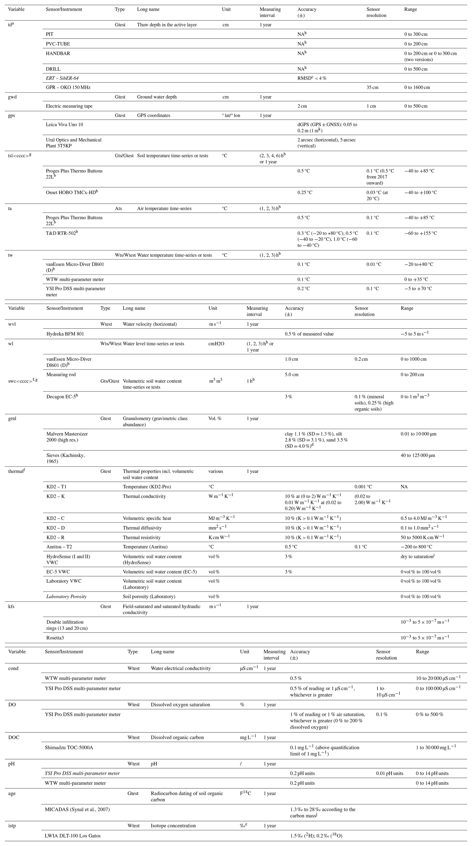
^a td represents thaw depth to frozen layer and differs from actual active layer thickness (see Sect. 4.1.3). Interpretation using electrical resistivity tomography (ERT) and ground penetrating RADAR (GPR) is subjective as it depends on relative signal strength changes.
^b Time-series.
^c RMSD – R mean squared difference between observation and interpreted td as presented in Léger et al. (2023).
^d Estimates from Miller and Schaetzl (2012). SD – standard deviation.
^e δ  notation with respect to Vienna Standard Mean Ocean Water (VSMOW).
^f Note that one-time swc tests/measurements are included in the thermal files.
^g <cccc> indicates the depth of time-series measurements in cm, using a 4 digit number with leading zeros, e.g. “0400” for a measurement depth of 400 cm.
^h Method accuracies and resolutions are subjective and should be seen as rough estimates and might have varied based on individual operators.
ⁱ For standard soil types in the range of 0 % to 50 % but can be higher for high porosity organic soils as e.g. in the soil pits near the river.
^j Accuracy refers to the entire ¹⁴C measurement process, including statistical counting, blank subtraction, and normalization using Oxalic Acid I. It does not reflect the intrinsic accuracy of the atomic mass spectrometer instrument only.
^k Observed differences in known instrument locations between different years showed differences of up to 1 m (see Sect. 4.4.2 for details).
NA: not available.

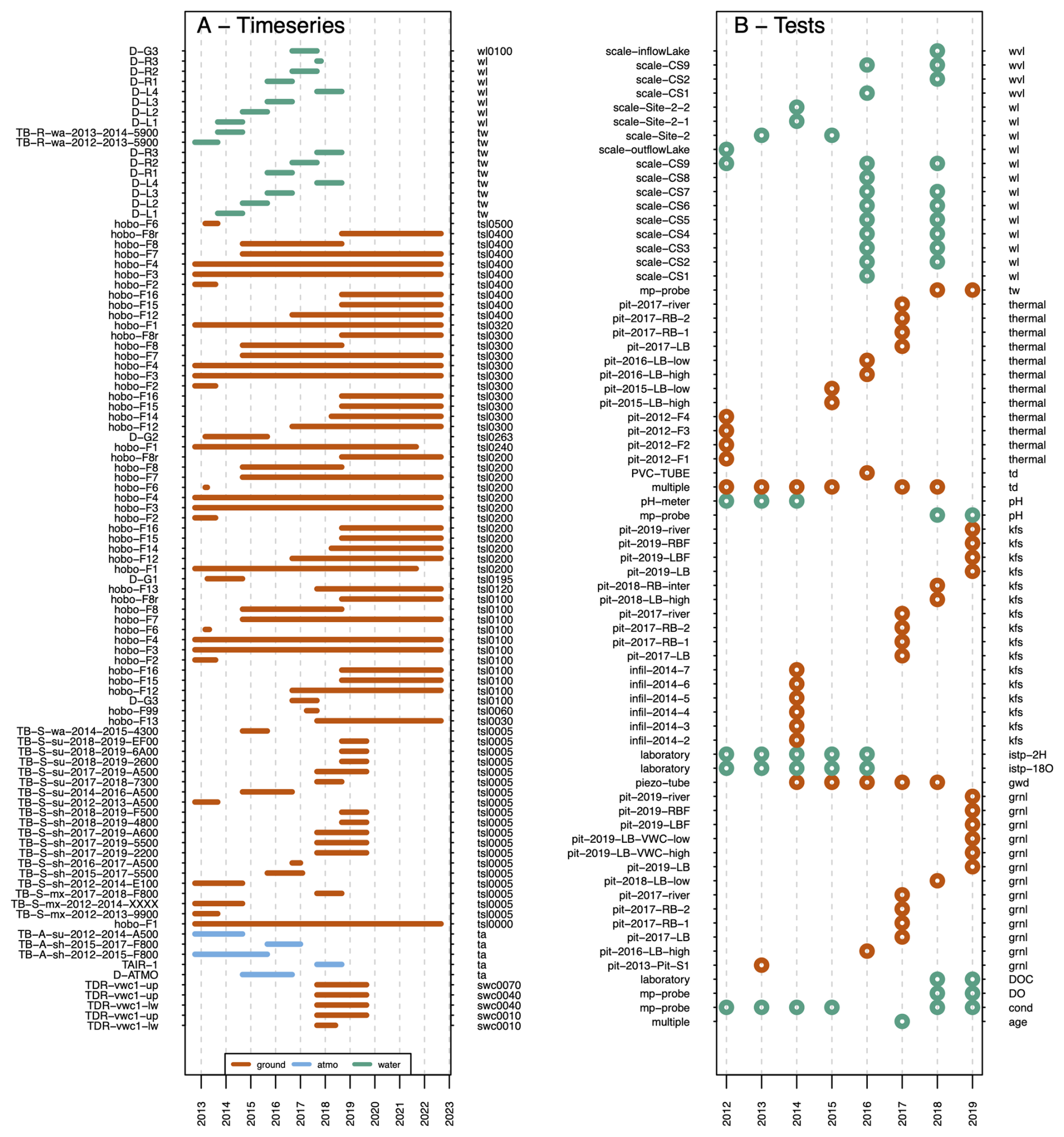
Figure 3 Temporal and variable type coverage of the dataset for (A) time-series and (B) individual tests. Left-hand side indicates the location and right-hand side (color-coded) the variable. See Table  for complete variable names.

3.1 GIS database

The database comes with a QGIS (QGIS Development Team, 2024) project file (.qgz) that displays all sampling and measurement locations (Fig. 1). In several cases, multiple instruments and/or measurements at various depths were employed/taken at a single point. In this case, the feature (point, lines, and polygons) name will reflect the common measurement location, e.g. “pit” (soil pit), “CS-i” (cross section i), or “piezo” (piezometer tube). The location where each measurement was taken is part of the filenames and facilitates identifying the measurement location. Data files that contain data from multiple measurement locations use the exact location names in the column “point” (e.g., isotopes, water conductivity measurements). The GIS database and contained imagery use by default an UTM zone 52N projection with the WGS84 datum.

3.2 Locations of observations

The compilation of measurement points over multiple years made use of a differential GPS (dGPS), a theodolite, and handheld GPS instruments (see Sect. 4.4.2 for details). The accuracy and precision of instruments to obtain measurement locations varied between instrument types and between years. To obtain a coherent set of coordinates, we aligned all points relative to the imagery obtained with an Uncrewed Aerial Vehicle (UAV) (Sect. 4.4.1) inside the GIS database. We prioritized having the measurement locations placed correctly relative to the landscape features in the UAV imagery, e.g., having a water level sensor being placed centered in the river, or having a ground surface temperature logger at the transition from meadow to forest being placed at this identifiable transition in the imagery. The feature vector files holding the positional information are described in Sect. 4.4.4.

The resulting coordinates can be extracted manually or using a provided Python script (Sect. 4.4.7). Making use of this, the user can adjust the locations for experiments by editing the feature shape files and creating their own coordinate lookup table using the script. This also facilitates the generation of figures requiring the spatial information (Sect. 4.4.3).

For river cross section water depths and velocities, relative positions from one shoreline to the other one, or with respect to the river position are reported in the CSV files; these dimensions might not match the provided UAV imagery as the width of the river might have changed between years. In each of the individual data files the location name is mentioned so that users can adjust such a profile according to their application needs with relevant information of the surrounding landscape available in the GIS database.

3.3 Database structure

The database is provided as a folder structure with most files in a simple CSV format in UTF-8 text encoding, imagery is provided as GeoTiff, vector files as GeoPackage, Ground Penetrating RADAR (GPR) data in SEGY format, and electrical resistivity tomography (ERT) data as inversion output from using the BERT software (Günther and Rücker, 2012), and programming and processing code in the form of R and Python scripts. The simple file format provides a way to present data sufficiently and without proprietary software for the different types of measurements (e.g. time-series vs. snapshot experiments in soil pits). The main subdivision of the database follows the different domains in which measurements were taken according to the following 4 main categories: ground, atmo(sphere), water, and auxiliary.

Filenames are constructed to provide the most important information about the measurements using the filename structure: $<variable\mathit{\_}id>\mathit{\_}<table\mathit{\_}id>\mathit{\_}<experiment\mathit{\_}id>\mathit{\_}<location\mathit{\_}id>\mathit{\_}<process\mathit{\_}level>\mathit{\_}<time\mathit{\_}range>.csv$, where variable_id is the short variable name (see Table ), table_id is the type of measurement (time-series $<x>$ ts, or tests $<x>$ test, for atmosphere (x=A), water (x=W), and ground (x=G)), experiment_id is the site descriptor (“syrdakh”), location_id is the name of a measurement point or static instrument if a single instrument is installed, process_level indicates if data is provided in raw format (L0), if instrument output is used as is without post-processing (L1), or has been post-processed (L2), and time_range provides a time range (time-series), or a year with the addition “-mean” to indicate a single measurement as is the case for most of the tests. The incorporated dataset by Hughes-Allen et al. (2020) is indicated with “sample-HA” as location_id and provides the seasonal information when the sampling took place, as an additional column in the data file. If precise time information was available, this is provided within the meta-data inside the file header.

3.4 Data files

In addition to the information included in the filename (Sect. 3.3), an extended header of 22 lines includes metadata, some of which are extracted from Table . An example of a header including corresponding data for a time-series as well as multi-point groundwater measurements is provided in Table B1. For time series, line 19 is used for a short description of the quality flags (see Sect. 3.5). The main data body varies depending on the type of data. Data not categorized as auxiliary are either time-series or tests (Table ). All time-series are three column files with date and time in the first, data values in the second, and a quality flag (Sect. 3.5) in the third column. The structure for tests varies depending on the type of data and is explained in the respective subsections for individual variables.

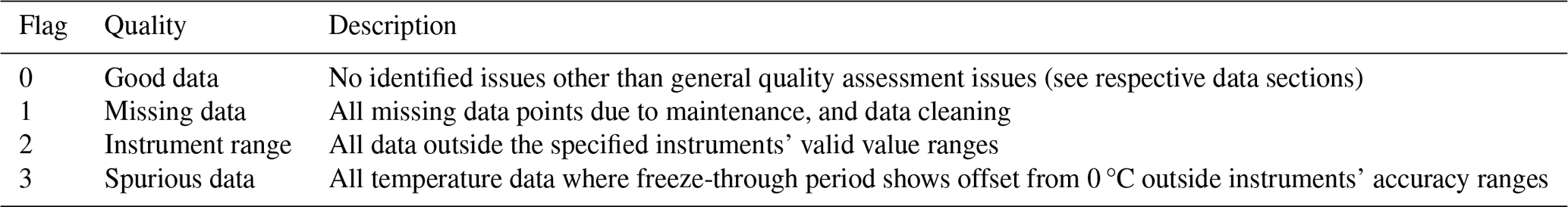
3.5 Data quality assessment

Each time-series was checked automatically to flag data outside the valid instrument ranges and missing data, as well as manually to identify spurious data (Table 2). Spurious data are data points for temperature time-series that show a deviation from 0 °C during the freeze-through period exceeding the instrument accuracy, or when temperatures exhibit a constant-rate (linear) change over time, which occurred only once. Quality flags are provided in the time-series data files as a separate column (“QF”). Additional information on flagging data as spurious is provided in the relevant section. For the tests, a quality assessment is given in the relevant sections. The assessment is based on field observations from independent datasets, experiences in the field, and assumptions on expected value ranges that are explained in the relevant sections.

Table 2 Data quality flags “QF” of time-series data.

4 Data description

4.1 Ground measurements

Ground measurements refer to any experiments and monitored time-series in the ground or at the ground-atmosphere, or ground-water interface and are stored in the main category “ground”.

4.1.1 Ground temperature – “temp”

Ground temperatures at various depths and at the water-ground interface were measured continuously with three different devices (Fig. 4). These are (1) Proges Plus Thermo Buttons 22L temperature loggers (TB) for measurements at the surface in around 5 cm depth, (2) van Essen Micro-Diver DI601 (D) installed at the water-ground interface to simultaneously measure water level as well as water-ground interface temperature (or surface air temperature in case of drying out of the rivers), and (3) Onset HOBO TMCx-HD Water/Soil Temperature Sensors as thermistor chains in combination with Onset HOBO U12 4-External Channel loggers (HOBO) for measurements at various depths, ranging from 5 to 500 cm. The measuring intervals varied depending on instrument type and depth between 1 to 6 h (Table ). Different intervals can be present in a single time-series (e.g. due to logger configuration changes), indicated in the header of the CSV files. All temperature measurements are stored in the category “ground/temp”. The HOBO thermistor chains were pre-assembled (Fig. D5) before installation in boreholes of 66 mm diameter. For this, four thermistors were typically wired and fixed at predefined distances from each other using tape to match the desired depths. The wired and length-fixed constructions were then placed inside PVC tubes matching the borehole diameters, with the lower sensor firmly fixed. Afterwards, a PVC plug was soldered to the lower end of the tube and the entire interior of the tube was filled with dry sand. A schematic cross-section overview of the installation in the cross-sections is provided in the Appendix (Fig. D6).

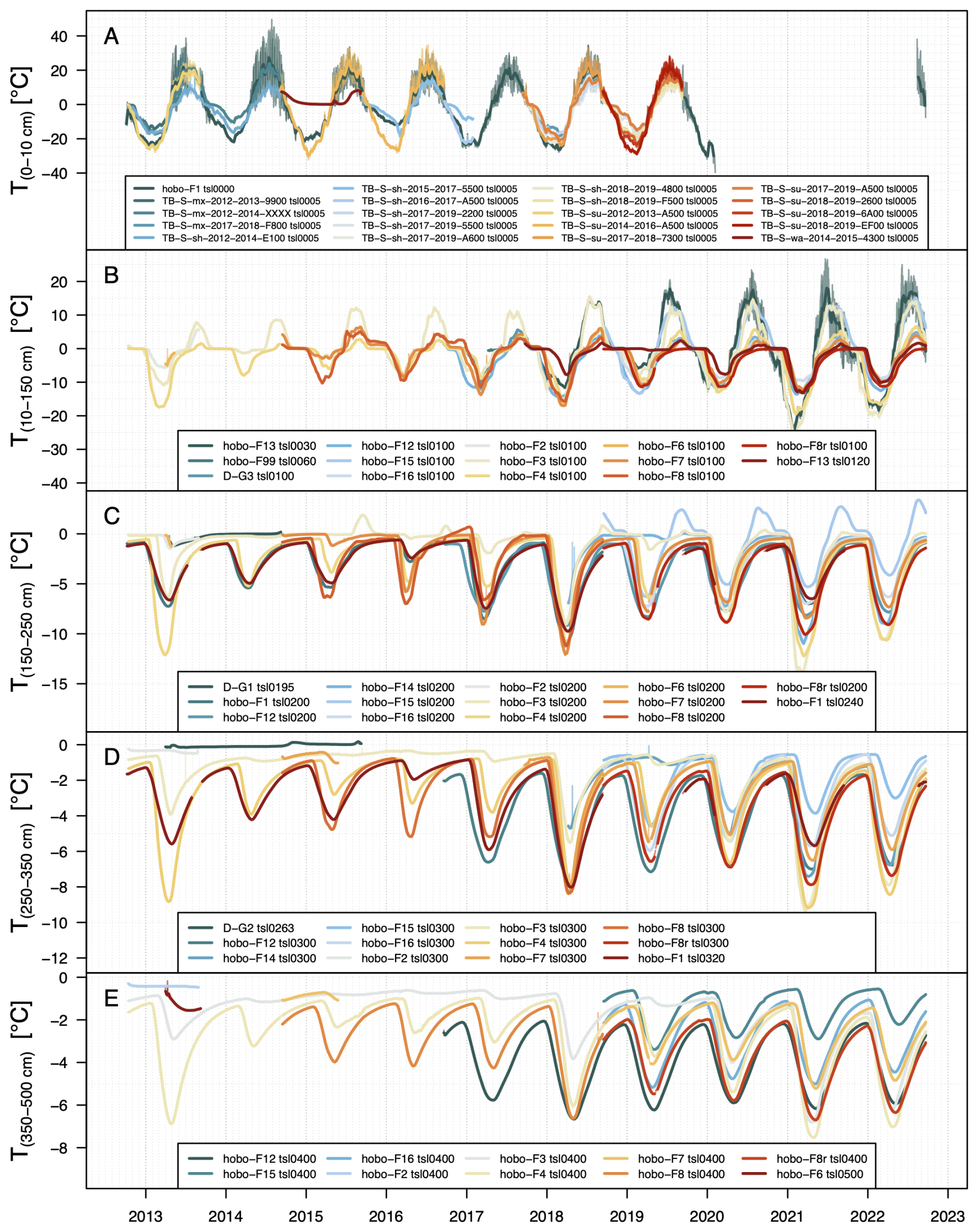
Figure 4 Ground temperature time-series for different depths (A–E). Measurement depths are indicated in the subscript of axes labels and in the variable names within the figure legends, e.g. “tsl0200” is at 200 cm depth. Ground near surface temperatures are mainly TBs (A). Identified data issues are mentioned in the main text.

The TB loggers were installed at various positions to provide temperature boundary conditions for numerical modeling. They cover a large range of land surface and vegetation covers, shadings, and terrain expositions. The instrument names together with the two element location_id reflect the main position (R-river, S-soil, A-air) and dominant exposure (su-sun, sh-shade, wa-water/wet, mx-mixed or unclear). TBs have been installed on around 20 cm long pegs made of wooden branches with the TB attached to the pegs (Fig. D1).

HOBO loggers were installed at the two main cross sections (CS) CS-2 and CS-9 (Fig. 1). The main purpose of the HOBO time-series is the monitoring of active layer and permafrost temperatures. HOBOs were installed in boreholes, drilled with a gas-powered auger (Fig. D2). Some attempts were made to install thermistor chains in the river bed but the instruments always broke, possibly as a result of cable shear stress when the river was frozen. All Divers (D) were located at the bottom of the river or lake and the temperature thus represents the interface temperature. While the lake never encountered freeze-through, the river measurements showed prolonged zero-curtain periods, followed by negative temperatures (Sect. 4.3.1).

Uncertainty and errors

All temperature time-series were manually checked for plausibility by comparing the temperature records during the freeze-through period with expected 0 °C values. None of the TB sensors showed a deviation higher than their accuracy. Issues were apparent for the HOBO data for “tsl0200_hobo-F8” in late 2016, and “tsl0200_hobo-F15” in autumn and winter. These data were flagged as spurious.

The TB data were analyzed regarding the minimum and maximum temperatures during the freeze-through period. They show a total value range between −0.2 and 0.2 °C for the maximum temperatures with a standard deviation of 0.07 °C, and a range between −0.5 and 0.1 °C for the minimum temperatures with a standard deviation of 0.23 °C (n=21).

The HOBO data show a total value range between −0.12 and 0.6 °C for the maximum temperatures with a standard deviation of 0.21 °C, and a range between −0.6 and 0.51 °C for the minimum temperatures with a standard deviation of 0.3 °C (n=16). The temperature signal of several HOBO time-series spiked in spring and are visible through multiple soil layers. Temperatures return to their original background level or trajectory after these occurrences. Such features have been associated with infiltrating melt water from snow melt as pointed out in other studies (Vonder Mühll et al., 2004). Here, such occurrences were not flagged as spurious.

4.1.2 Thermal properties – “thermal”

Thermal properties were determined using a KD2 Pro Thermal Properties Analyzer from Decagon Devices with a 3 cm dual-needle (SH-1) sensor. Properties were measured in situ in soil pits (Figs. 1, D3), as well as from soil samples that had been taken and analyzed in a laboratory at the Melnikov Permafrost Institute (MPI), Yakutsk, or in a laboratory of the Laboratoire des Sciences du Climat et de l'Environnement (LSCE), Paris. Temperatures at the measurement locations were additionally measured using an Anritsu HD-1200K thermometer (Anritsu Meter Co.) (Table ). The thermal files include in situ volumetric soil water content (SWC) measurements (Sect. 4.1.4), providing basic information for the parameterization of ground properties for hydro-thermal modeling. In case SWC was determined from soil samples in the laboratory, soil porosity estimates are provided as well (Sect. 4.1.4). The file structure provides the results for each variable within “thermal” (Table ) as separate column for the individual depths (rows) of a soil pit.

Uncertainty and errors

Errors might be present in the calculation of thermal properties using the KD2 Pro device. This is because the KD2 Pro temperature measurements showed significant differences to the Anritsu thermometer (Fig. 5). The manual of the KD2 Pro highlights that the relevant formulas for the calculation of thermal properties use changes in temperature during the measurements rather than absolute temperatures (Decagon Devices Inc., 2016), thus a constant bias in the temperature measurements would not affect the calculation. If the temperature offset, however, indicates a more severe issue with the KD2 Pro temperature, this could mean that derived thermal properties were affected. As we did not conduct any controlled experiments on this issue, we cannot assess the potential scale of the error. The accuracy of the thermal parameters (other than stated in Table ) could therefore not be assessed as the relevant information is not publicly available. The obtained value ranges for the different soil grain size compositions and SWC contents are similar to values obtained in other studies in the region (Zhirkov et al., 2021).

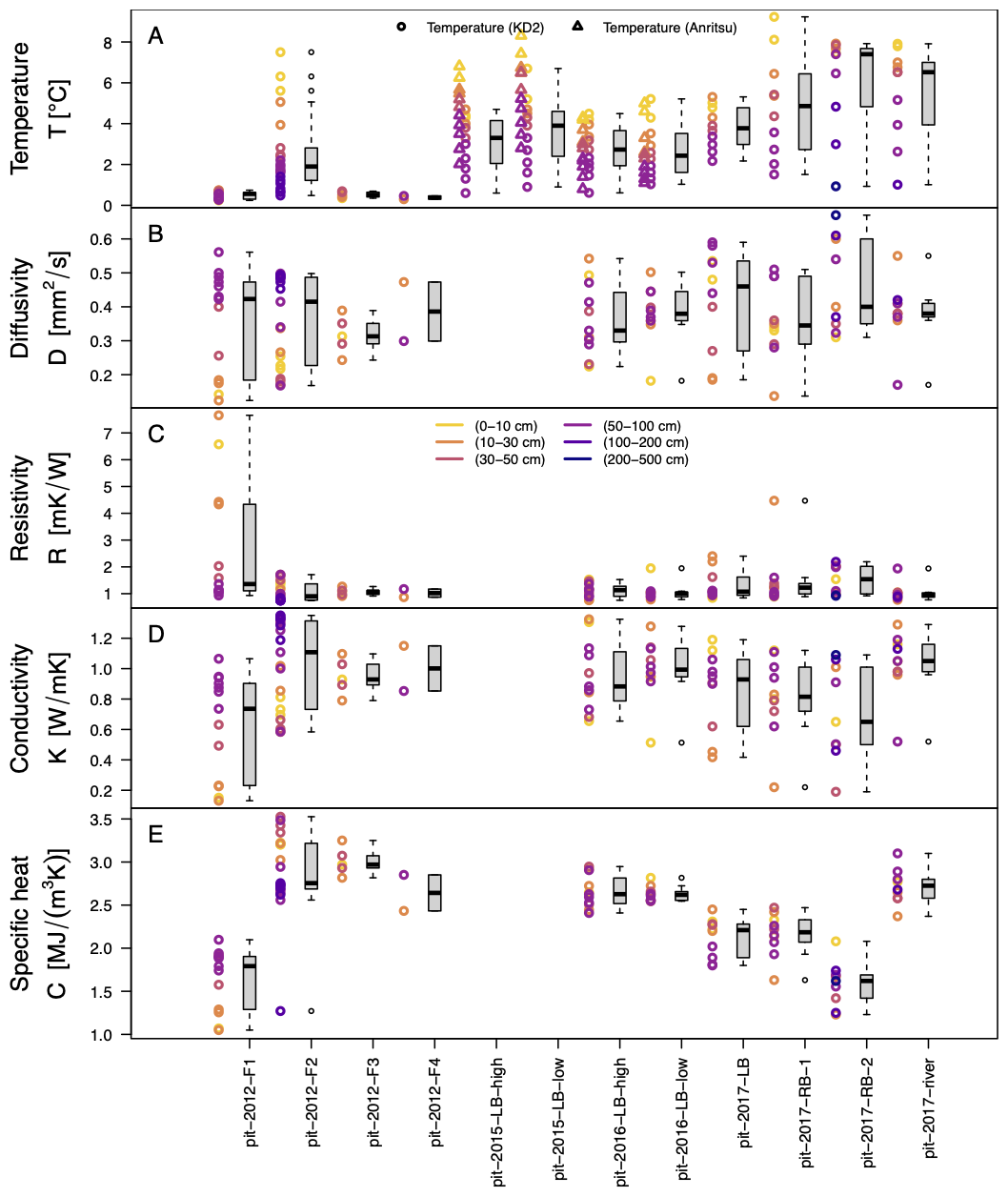
Figure 5 Various thermal properties (A–E) of soil samples analyzed in situ in various soil pits.

4.1.3 Thaw depth measurements – “td”

The ground temperatures (Fig. 4) indicate a downward heat transfer in the active layer and its thawing that lasts until September or October, with differences among sites (Fig. 6). The field campaigns were usually conducted late September for logistic reasons. As a consequence, what we report here are thaw depths in the active layer rather than absolute active layer thicknesses. The thaw depth does not necessarily represent the maximum thaw depth but only the depth to the frozen layer at the time of the measurement. The time of measurement is included in the individual data files as well as in the relevant geopackage files in the GIS database.

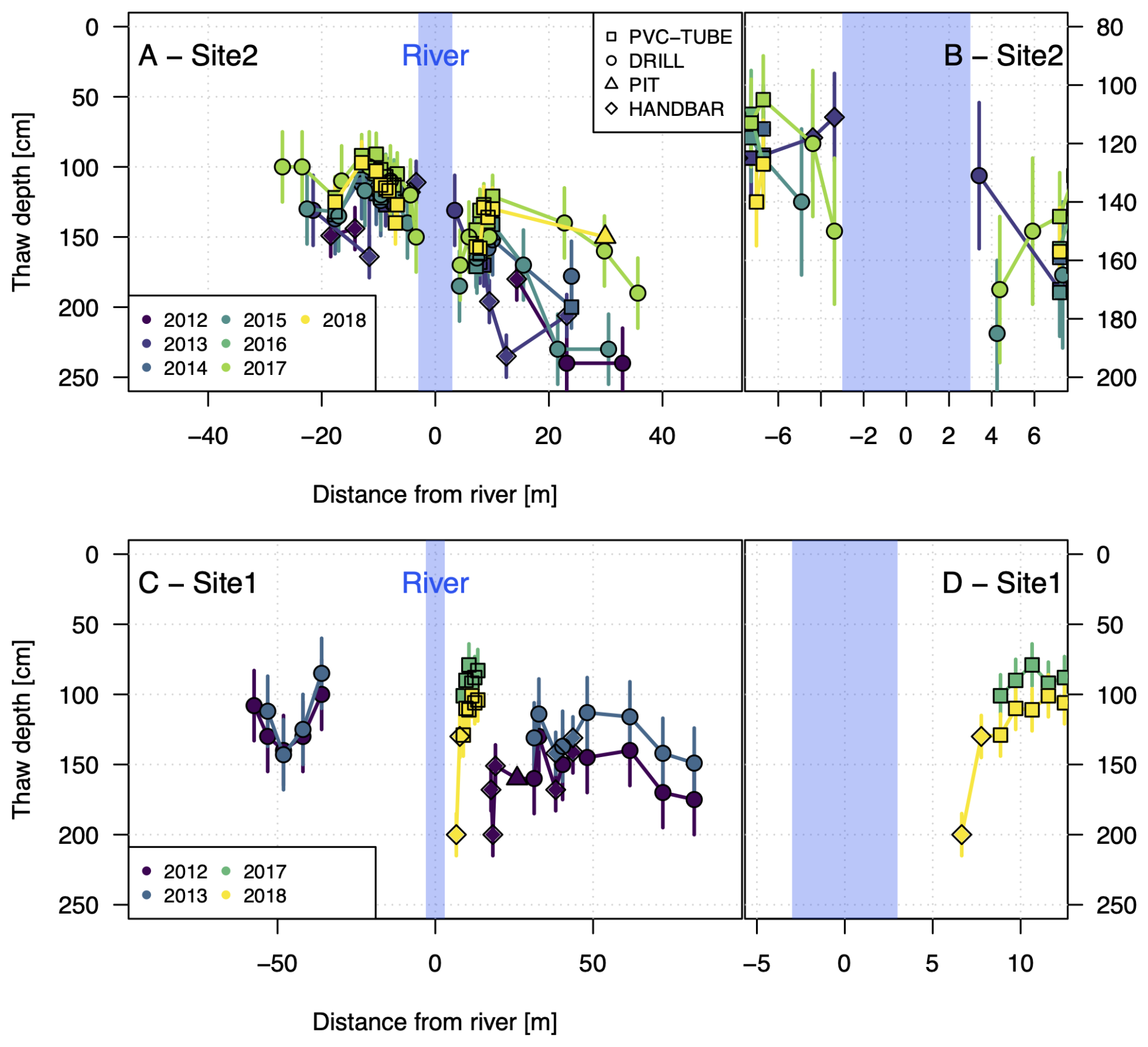
Figure 6 Thaw depths in the active layer at two cross-sections at the two main locations Site 2 (A) and Site 1 (C) with zoomed-in detail views (B and D, respectively). Each point represents a single measurement. Error bars represent unverified assessment of measurement errors of different techniques as explained in the text. Date of measurement for individual years varied – information is contained in the data files and in the geopackage files of the GIS database.

The depth was determined using different methods, including probing with metal rods, and drilling (Fig. D2), and as part of an independent study (Léger et al., 2023), by means of electrical resistivity tomography (ERT), and ground-penetrating radar (GPR) (Fig. C1). The data of Léger et al. (2023) are provided in the “auxiliary/external/” folder (see Sect. 4.1.3). The regular td data files have four columns that provide, in addition to the location and the td determined, information on whether the maximum probing depth was exceeded (“max_exceed”), and the method used to determine the td (see Table ).

Drill and probing rods

The depth to the frozen layer was determined by pushing a metal rod into the soft soils or through the piezometer tubes which extend through the active layer. Probing in the compacted soils on the right-hand side river bank was often not possible and a drill was used instead (Fig. D2).

Ground Penetrating Radar (GPR)

Two ground-penetrating radar (GPR) prospecting campaigns were conducted in October 2017 and October 2018, when the upper thawed layer depths were at their annual maximums, just before the onset of the freezing period. GPR data were acquired in the time domain using the Russian OKO system, comprising one set of antennas centered on 150 MHz. In October 2017, the river had mostly dried out in its narrower part, allowing for the use of the GPR with facilitated access to the riverbed in the cross-section CS1. In contrast, on CS2, the data were acquired on each side of the water pond (water level approximately 50 cm at its deepest point). For all GPR data, the spatial sampling interval was set to 0.02 m, the time sampling interval was set to 0.39 ns, and the time window was adjusted to 100 ns. Further details can be found in Léger et al. (2023).

Electrical Resistivity Tomography (ERT)

Electrical Resistivity Tomography (ERT) data were acquired using a 16-channel SibER-64 system with 64 electrodes and a 0.5 m spacing between electrodes, using Dipole-Dipole, Schlumberger and Wenner configurations. Using a roll-over procedure, we were able to obtain a 63.5 and a 71.5 m long transect for CS1 and CS2, respectively. The transect for CS2 was collected in 2018 and for CS1 in 2017 and 2018. Data processing was performed prior to the inversion consisting mainly of removing extreme contact resistance values due to bad contact with the ground. Data were inverted using the finite-element inversion program BERT (Günther and Rücker, 2012) to obtain the spatial distribution of soil electrical resistivity, and including topography. We used a robust inversion (L1-normalization), giving a higher probability to obtain blocky models with sharp boundaries. Further details can be found in Léger et al. (2023).

Uncertainty and errors

The determination of thaw depths using any of the applied methods were subject to different sources of error and varying uncertainty. The determination with metal rods in soft soils was feasible as the frozen ground provided a significant change in hardness that could easily be determined when inserting the metal rod into the ground or piezometer tubes. On the right bank near CS-9, very compacted soils prevented using the rod. The determination of the frozen boundary from drilling was subject to the experience of the drill operator. All mechanical measurements have been somewhat validated in two years when soil pits were dug next to the td measurements. We assumed maximal uncertainties in the range of ±2 cm for soil pits, ±15 cm for piezo tubes and metal rods pushed by hand, and ±25 cm for the mechanical drill. GPR- and ERT-derived estimates are in agreement with the manual estimates within the uncertainties in interpreting where the frozen layer starts from the non-invasive geophysical methods (Léger et al., 2023).

4.1.4 Soil water content – “swc”

In situ soil water content was measured with a permanently installed system for obtaining time-series since 2017, and in soil pits in different years. For soil pit measurements, the main instrument was a HydroSense I and later a HydroSense II (Campbell Scientific) time domain reflectometry (TDR) device. Regarding their performance, the only difference is an improved accuracy for HydroSense II for very high electrical conductivity (electrical conductivity > 2000 µS cm⁻¹). High volumetric water contents outside the regular measuring range (0 % to 50 %) were obtained in high organic, and porous soils near the river and below the river bed, and were also independently calculated from soil samples in the laboratory (Fig. 7). The time-series were obtained using EC-5 TDR probes (Decagon Devices) in depths of 10 to 70 cm, connected to a Decagon Em50 data logger. The probes were installed on two opposing sites of a soil pit made in 2017 on the left river bank. One side of the pit (“TDR-vwc1-lw”) is lower and closer to the river, whereas “TDR-vwc1-up” is located about 2 m further south, further away from the river, and slightly higher in elevation. These probes were tested in 2017 against the HydroSense II TDR probe that was used in all other years (Fig. 7). Analyses in the lab were conducted following a standard workflow of 100 mL sample weight measurements before and after oven drying at 105 °C for 24 h, following the standard by the American Society for Testing and Materials (American Society for Testing and Materials (ASTM), 2019).

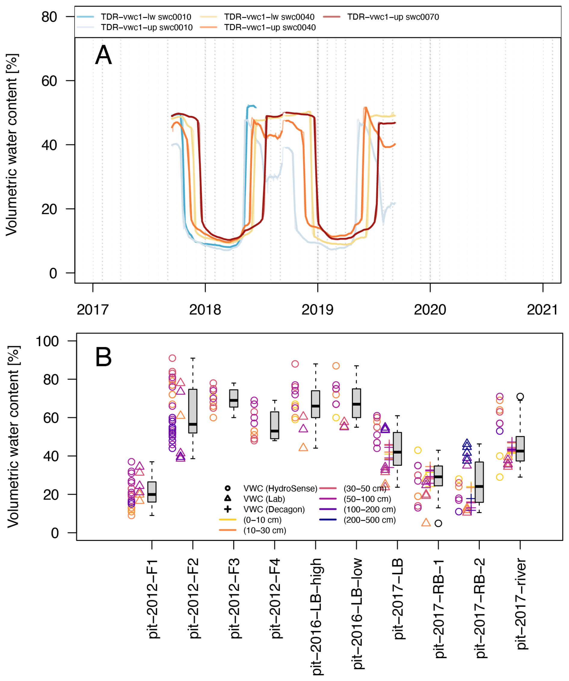
Figure 7 Soil water content measurement time-series using EC-5 probes from Decagon (A), and individual tests made in soil pits or from soil samples analyzed in the field and the laboratory using multiple instruments (B).

Soil water content is provided as volumetric water content (VWC). The data from the Em50 data logger were transformed into VWC using Eq. (1):

$$\begin{array}{}\text{(1)}& \mathrm{VWC}=(\mathrm{8.5}\times {\mathrm{10}}^{-\mathrm{4}})\cdot \mathrm{RAW}-\mathrm{0.48},\end{array}$$

where RAW is the output from the Em50 data logger, as referenced in the EC-5 Manual (METER Group Inc., 2023). The HydroSense instruments provided VWC estimates without any calibration having been performed. Within the “thermal” files, laboratory estimates (see comparison in Fig. A2), as well as EC-5 probe estimates are provided for an idea of accuracy. Snapshot measurements (tests) in the soil pits are included in the “thermal” files under the columns “VWC HydroSense” for the HydroSense estimates, “VWC EC-5” for EC-5 probes, and “VWC Laboratory” for the laboratory measurements at MPI or LSCE.

Uncertainty and errors

The TDR-derived VWC estimates are based on changes of the probed material's dielectric property and the instrument's internal calibration (VWC HydroSense and VWC EC-5). Therefore, differing soil types resulted in different results. Figure 7 shows that near the position of the continuous TDR installation “TDR-vwc1” at “pit-2016-LB”, the laboratory derived estimates were consistently lower (about 40 vol % to 60 vol % vs. 60 vol % to 80 vol % for “VWC HydroSense”). The continuous TDR-based estimates of “VWC EC-5” range between 35 vol % to 55 vol % (at position “TDR-vwc1”). In different tests, where the “VWC EC-5” sensor was used, no systematic over- or underestimation could be identified, neither between the HydroSense and the laboratory estimates (Fig. 7). A maximum disagreement between individual measurements is about 30 vol %.

4.1.5 Soil composition – “grnl”

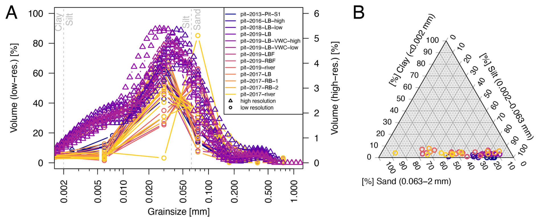
Grain size distributions were measured until 2017 at MPI and classified mostly using the Kachinsky classification (Kachinsky, 1965) with around 10 relevant grain size classes. Grain sizes were determined using sieves with mesh sizes according to this classification (Kachinsky, 1965). The reporting classes for 2013 deviated from other years for the two finest grain size classes (0.01–0.005, and <0.005 mm as compared to 0.01–0.002, and <0.002 mm). Some samples after 2017 were measured using a laser diffraction grain size analyzer Mastersizer 2000 HYDRO-G (Malvern) that provides a discrimination into 100 classes. Without relevant information available to homogenize these classes, we provide the classes as they were reported. For the file structure, this results in relevant grain size classes in one column and their respective wt % in a separate column; each measurement depth within a soil pit is reported as a single column. From 2012 through 2019, one or multiple soil pits were dug each year, but granulometric analyses were not performed each year.

Uncertainty and errors

A comparison between the sieve- and diffraction-based results shows differences, particularly for the silt fractions (Fig. 8). As none of the samples had been measured with both methods, it remains speculative whether the differences represent a real difference in grain size distribution or whether this is the result of the method. The determined soil classes correspond to sandy silt, or silty sand soils (Fig. 8), which has also been reported by other studies for cryospheric soil types in the region (Zhirkov et al., 2021; Desyatkin et al., 2021).

Figure 8 Grain size distributions (A) of soil samples and corresponding ternary plot (B).

4.1.6 Hydraulic conductivity – “kfs”

Hydraulic conductivity, either field-saturated or saturated (kfs), were estimated using two different methods. Multiple water infiltration tests were performed in soil pits to determine field-saturated hydraulic conductivity. For the years 2012 through 2016 only infiltration tests with two metal rings (13 cm inner and 20 cm outer diameter) were performed. Metal rings were pushed several millimeters into the upper soil and infiltration was measured for falling head conditions. Measurements were taken with respect to the upper edge of the inner ring and written down every few seconds to every few minutes the longer the experiment would run. Regression over the quasi-linear part for field-saturated conditions were reported. In addition to the in situ infiltration tests, for the samples from 2017 through 2019, grain sizes were determined from soil samples in the laboratory (Sect. 4.1.5) to derive the saturated hydraulic conductivity using the Rosetta3 algorithm (Zhang and Schaap, 2017). The applied method for the determination of kfs is reported in a separate column (“method”) in the relevant files.

Uncertainty and errors

The highly compacted soils on the right bank required mechanical work to insert the infiltration rings into the soil. While no direct leakage was visible as a result of this, such leakage would result in overestimated infiltration rates and kfs. The comparison of kfs of the right bank showed in fact higher kfs compared to some of the river and left bank experiments (Fig. 9). However, the latter had experienced highly saturated conditions that might have caused the low values. For such saturated conditions, single sites (e.g. “pit-2019-LB”) show a significantly wider range in kfs values, which can span one order of magnitude.

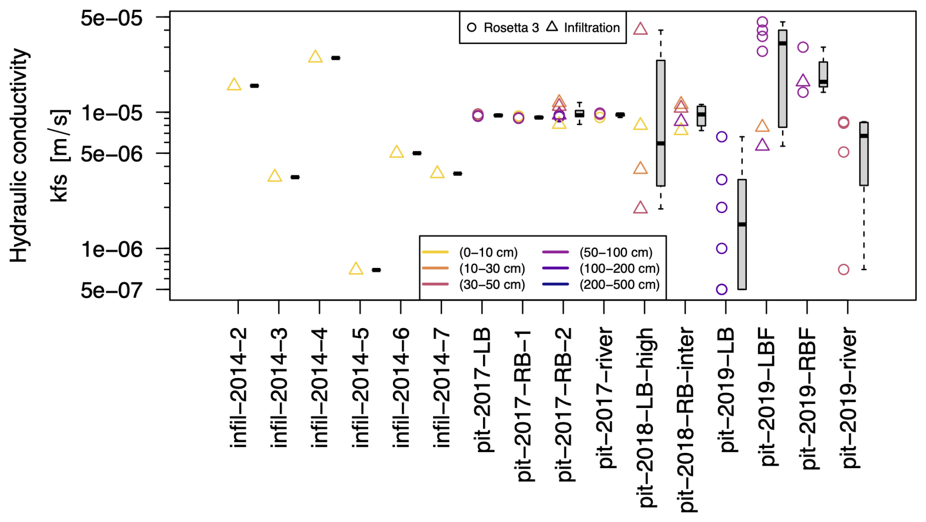
Figure 9 Hydraulic conductivity estimates determined by infiltration tests (field-saturated) and laboratory analysis of grain size distributions using the Rosetta3 algorithm (saturated, Zhang and Schaap, 2017), at the surface and various depths within soil pits.

4.1.7 Ground water depth – “gwd”

During the end of summer field campaigns, attempts were made to measure the water table height inside the piezometer tubes near CS9 and CS1. The ground water level was determined by using an electrical measuring tape, identifying the distance between wet tape and top of the piezometer tubes. The distance was adjusted for the height of the piezometer tubes above the land surface.

Uncertainty and errors

The piezometer tubes were installed in drill holes that reached the frozen layer. Consequently, the hydraulic head measured in the tubes might have been disconnected from the one in the thawed layer, and instead might represent the hydraulic head of a previous time period where the connection existed. An indication for an existing direct connection, however, is the year 2017, when the river mainly dried out and gwd showed the lowest values (Fig. 10). At the same time, the td was relatively shallow in comparison to other years (Fig. 6), suggesting no preferential hydraulic head connection compared to other years.

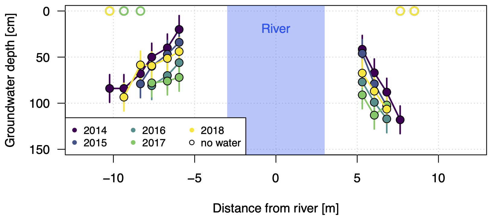
Figure 10 Groundwater depths measured in piezometer tubes at CS-9 using an electric measuring tape. Error bars represent a potential error of 15 cm (see uncertainty estimation), as was the case for the td measurements (see Fig. 6).

Additionally, some gwd measurements show a deviation from a gradient of continuously lower gwd with increasing distance from the river (Fig. 10). Based on these deviations, an error of around 15 cm is estimated.

4.1.8 Radiocarbon dating of soil organic carbon – “age”

Radiocarbon dating was performed on soil samples of four soil pits at Site 2 (Fig. 11). The dating data were obtained at LSCE following standard procedures. Soil (permafrost) samples were chemically prepared according to the protocols published in Hatté et al. (2024). The preparation involved decarbonation with 1 N HCl. Carbon-rich samples were subsequently oxidized into CO₂ and reduced to graphite carbon (Cgraphite) using an automated device (AGE; Wacker et al., 2010a). They were then introduced in the solid source of the MICADAS atomic mass spectrometer (AMS) instrument (Synal et al., 2007) operated at LSCE (Tisnérat-Laborde et al., 2015). Carbon-poor and small samples were introduced in an elemental analyser connected to the gas source of ECHoMICADAS, through a gas interface system (EA-GIS; Ruff et al., 2010). Raw data processing and reduction were carried out using BATS software (Wacker et al., 2010b) and a custom calculation procedure (Thil et al., 2024). Results are expressed in F¹⁴C and normalized to the international standard, Oxalic Acid 1. The CSV files contain all relevant information from the standard processing protocols (Hatté et al., 2024), as well as ages in years BP, which are calculated using the formula of Stuiver and Polach (1977):

$$\begin{array}{}\text{(2)}& \mathrm{Age}=-\mathrm{8033}\cdot \ln \left({\mathrm{F}}^{\mathrm{14}}\mathrm{C}\right)\end{array}$$

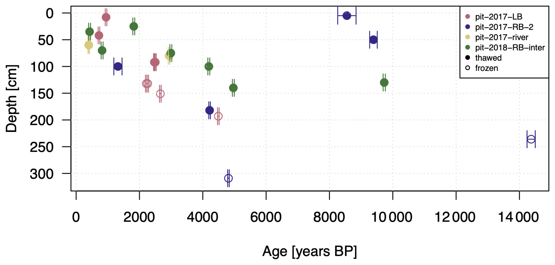
Figure 11 Radiocarbon dating (¹⁴C) at Site 2. Ages are derived from F¹⁴C using the conversion of Stuiver and Polach (1977) (see main text). Error bars represent ±1 standard deviation, calculated by first-order propagation of uncertainties through the logarithmic age transformation. Frozen samples likely represent permafrost; however, this interpretation is based on measured thaw depths rather than verified active layer depths (see Sect. 4.1.3).

Uncertainty and errors

Measurement errors or uncertainties arise from the statistical counting of ¹⁴C ions in the AMS (MICADAS) and from the propagation of errors during blank subtraction and normalization using Oxalic Acid I, the standard. Statistical counting depends on the sample mass and the measurement duration. Thus each individual age estimation is provided with an associated uncertainty in the respective files. Some old ages were apparent in the topsoil samples (“pit-2017-RB-2”). We do not investigate further the possible reasons for that but soil disturbances from road works and soil redistribution along the hillslope were visible in the field (Fig. D4). Deeper layers display continuously older ages and the frozen zone contained abundant ice lenses, both suggesting unlikely mobilization and disturbance of the soil substrate.

4.2 Atmospheric measurements – “atmo”

4.2.1 Temperature – “temp”

Air temperature was measured in the transition zone between the meadow and forest at Site 2 either with a TB (Sect. 4.1.1) in various years, with a T&D-502 temperature sensor (TAIR) between 2017 and 2018, or with a vanEssen Micro Divers DI601 (D) (same as in Sect. 4.3.1). All instruments were installed at 2 m elevation from the ground at an approximate elevation of 149 m a.s.l. TB and D loggers were attached to the north-facing sides of larch tree stems. All but two loggers were installed at the southern side of CS 9 at Site 2. These two loggers were installed near CS 2 at Site 1: one similar to the other loggers at the transition from meadow to forest in the southern part of the valley, and one in the open valley section at a free-standing tree.

TB and D loggers were installed with the exception of one TB (open valley section at Site 1) within the first few meters of the forest with a nail or a metal wire; the sensor of TAIR was attached at Site 2 underneath its logger housing box that was strapped to a tree a few more meters inside the forest. The sensors were installed north-facing to prevent direct solar insolation. There was no shielding installed against diffusive radiation nor against any other kind of external influence.

The closest long-term meteorological station is located in Yakutsk (Yakutsk – WMO ID = 24959, 103 m a.s.l.), around 100 km southeast. The data archive for Yakutsk was obtained via the website rp5.ru (Raspisaniye Pogodi Ltd., 2004) and is provided under “auxiliary/external”. A correlation analysis for the period 2017 through 2018 (Fig. A3) showed a coefficient of determination of 0.991. The Yakutsk data are provided to facilitate a continuous time-series analysis, as none of the here-presented measurements were continuous at any of the locations.

Uncertainty and errors

The low maximum sun elevation angle in Syrdakh of about 51° at summer solstice, together with the dense forest prevent any direct solar insolation; whether the air temperatures of the single TB instrument near Site 1 in the open valley section were affected by direct solar insolation was not tested. Riming and snow cover might have affected the measurements of the exposed TB and D sensors; snow cover could be excluded as an external factor on the measured air temperatures obtained with the TAIR sensor due to its sensor location underneath its logger box. For using an external time-series from a meteorological station with a longer record, the Yakutsk WMO station is a possible candidate. The high correlation of the data from this station with the local measurements supports the assumption of the regional climate influencing the local conditions in Syrdakh and support the use of the continuous time-series from Yakutsk for studies in Syrdakh after correction. However, stronger deviations were present in winter (Fig. A3). No analysis on possible reasons for the seasonal deviation has been performed.

4.3 Water measurements – “water”

While the focus of this database is revolving around the thermal evolution and properties of the ground, some chemical and physical analyses on the river, thermokarst-, and alas-lakes were conducted. However, a much more detailed analysis and database on river and lake physio-chemical properties exist (Hughes-Allen et al., 2020, 2021).

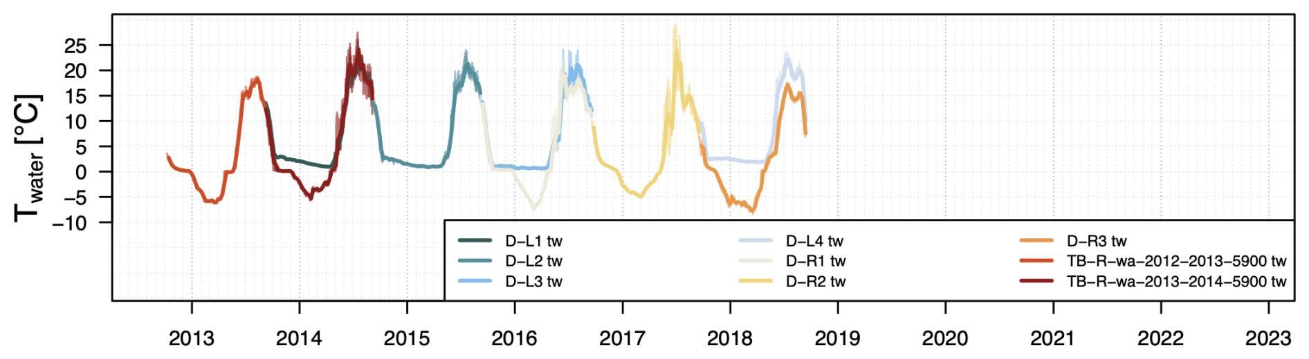
4.3.1 Water temperature – “temp”

Continuous water temperatures and water level were measured using vanEssen Micro Divers DI601 (D) sensors. The sensors were installed in the upstream lake, at around two meters general depth, deep enough to be below the winter ice cover. The sensors were held in place on the lake floor with a weighted bag, and secured with a rope approximately 2 m to 5 m away from the shoreline. Additional sensors were installed inside piezometer tubes located near CS-9 in the river bed as well as in a piezometer tube on land.

Figure 12 Water temperatures in the upstream lake and the river.

Uncertainty and errors

The water temperature data were analyzed regarding the minimum and maximum temperatures during the freeze-through period for the sensors located in the river and in the piezometer tubes (groundwater). They show a total value range between −0.01 and 0.31 °C for the maximum temperatures with a standard deviation of 0.16 °C, and a range between −0.03 and 0.1 °C for the minimum temperatures with a standard deviation of 0.16 °C (n=6).

4.3.2 Water electrical conductivity – “cond”

Electrical conductivity was measured on-site using a WTW multi-parameter meter (accuracies of ±0.1 °C for temperature, ±0.2 for pH value and ±0.5 % for specific conductivity) in 2017 or a YSI Pro DSS multi-parameter probe (±0.2 °C for temperature and ±1.0 % for specific conductivity) (Fig. 13). Again the interested reader is referred to the much more comprehensive dataset and study in the region by Hughes-Allen et al. (2021). Some measurements in thermokarst lakes obtained with the WTW multi-parameter meter exceeded the instrument's maximum electrical conductivity range of 2000 µS cm⁻¹.

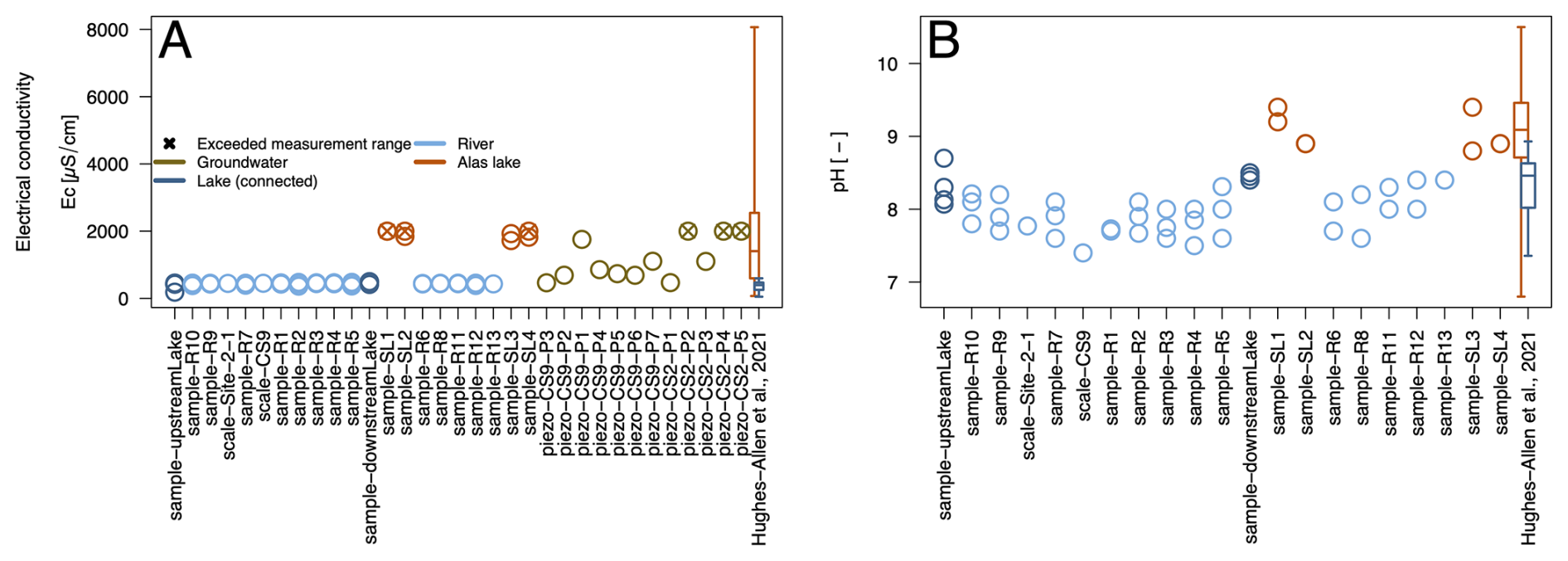
Figure 13 Water electrical conductivity (A) and pH value (B) of water samples. Additional analysis of lake samples from Hughes-Allen et al. (2020) and Hughes-Allen et al. (2021) are available in the respective datasets and publication.

Uncertainty and errors

The YSI multi-parameter probe was calibrated at the start of each field mission, but could not be calibrated daily due to logistical constraints. However, multiple calibration sessions over the years showed that the sensors, including the conductivity sensor, do not drift significantly.

4.3.3 pH values – “pH”

A YSI Pro DSS multi-parameter meter, as well as the WTW multi-parameter meter were used to determine the pH values.

Uncertainty and errors

As for conductivity (see above), the YSI multi-parameter probe was calibrated at the start of each field mission, but could not be calibrated daily due to logistical constraints. However, multiple calibration sessions over the years have shown that the sensors, including the pH sensor, do not drift significantly.

4.3.4 Water levels and depths – “levl”

Two types of measurement are in the following referred to as water level “wl” measurements. These include continuous monitoring of water column pressure in lakes, the river, and in piezometer tubes, as well as manual measurements of water depths using meter bands and measuring rods at selected cross-sections between the upstream lake outflow at Site 1 and the highly instrumented Site 2 downstream (Figs. 14, 15). The cross section location center points along the river for the manual measurements (Fig. 15) are referred to as “scale-CS” in the QGIS database and contained in the GeoPackage files (see also Sect. 3.1). Discharge measurements were conducted not in all cases when water levels were taken. Additionally, no flow conditions occurred in 2017, 2019, and 2021. Atmospheric pressure probes were only installed between September 2014 and September 2016 at location D-ATMO, at the same location as TAIR, and at an elevation of 2 m a.g.l. The data file is provided in “auxiliary/external”. In order to correct the water level loggers for the influence of atmospheric pressure in all years, we utilized hourly data from the Yakutsk meteorological station (World Meteorological Organisation ID: 24959, Raspisaniye Pogodi Ltd., 2004). For this, we first derived a relationship with the atmospheric pressure time-series taken in Syrdakh between 2014 and 2016 using a vanEssen Micro Diver DI601 sensor (D-ATMO). The correlation between the Syrdakh and Yakutsk meteorological station atmospheric pressure showed a coefficient of determination of 0.96 (Fig. A1). The obtained linear relationship was then used to adjust the atmospheric pressure of the Yakutsk meteorological station data. The data are provided in “auxiliary/external”. All water level data were corrected with so-adjusted atmospheric pressure data.

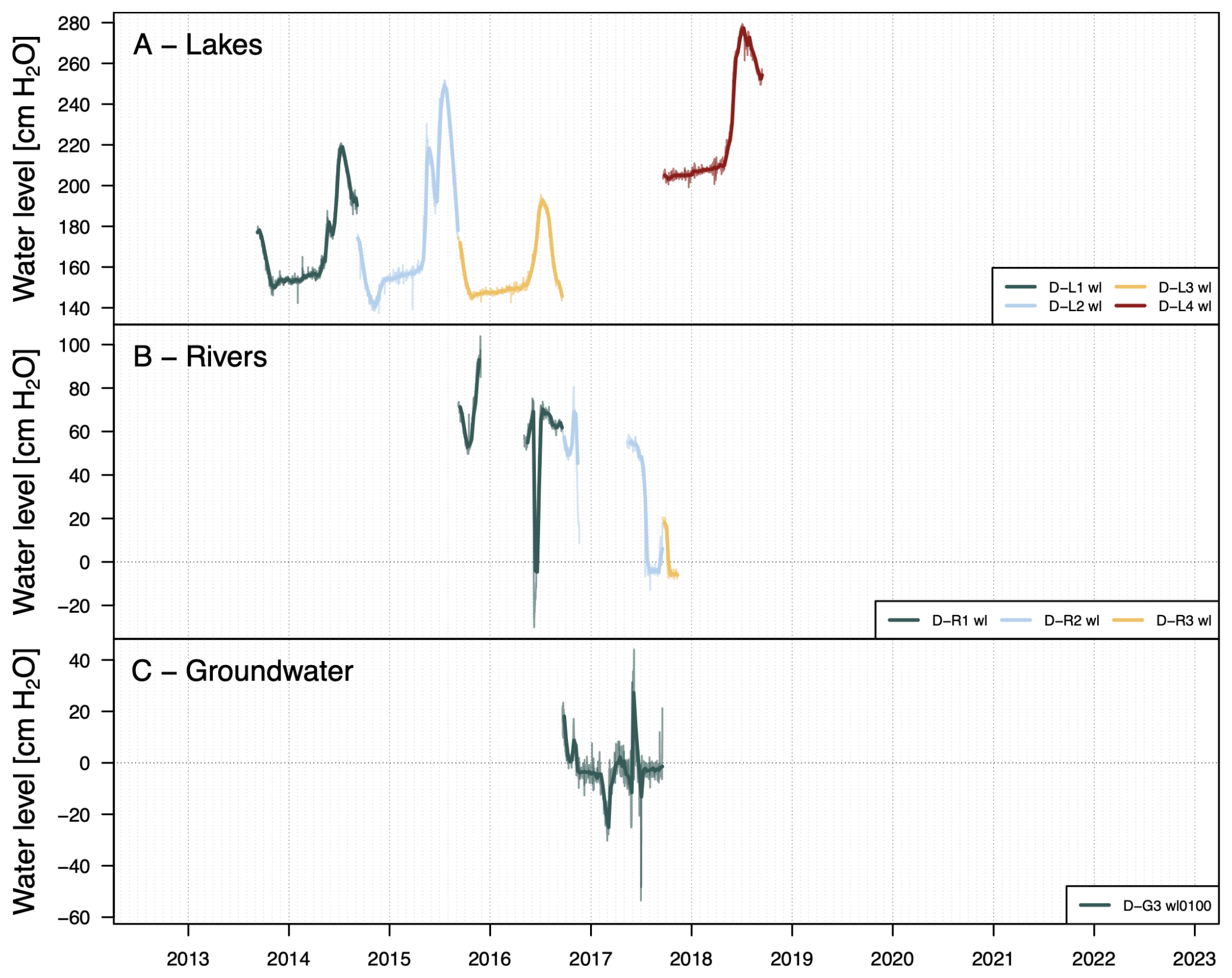
Figure 14 Water level measurements in the upstreamLake (A), in piezometer tubes along the river for river water level (B) and groundwater level (C). Extreme value differences for river and groundwater might indicate issues with pressure sensors due to freezing. Also visible are the continuous but slightly negative values around 0 cm for groundwater. It is unclear if this is a result of the extrapolated atmospheric pressure values based on the Yakutsk meteorological station (see text).

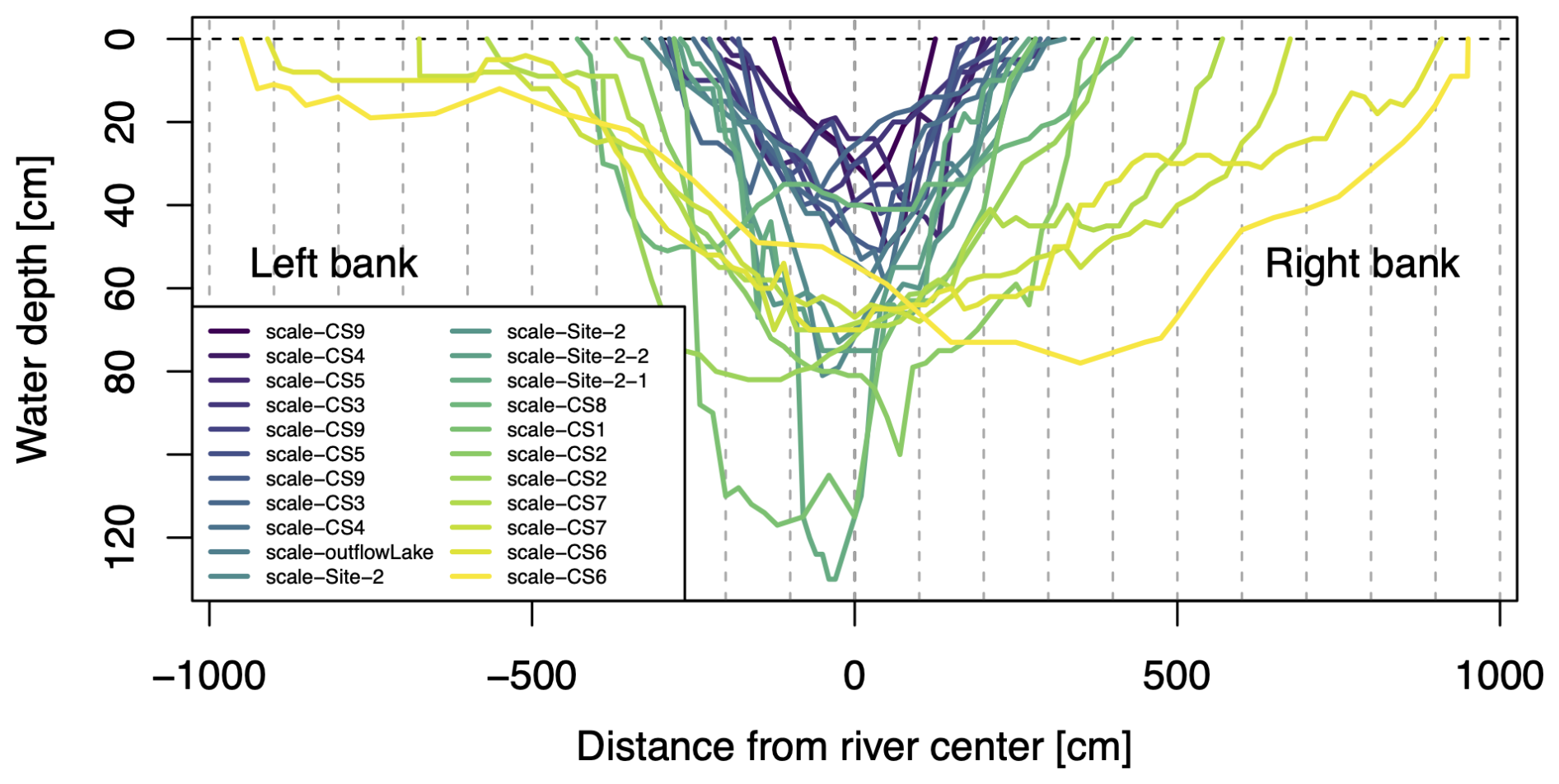
Figure 15 Water depths at cross sections along the river. Most of the profiles measured in 2018 at low flow conditions. Cross sections are ordered by cross section area. Left and right bank refer to downstream flow direction.

Uncertainty and errors

Data points were removed for when the temperatures showed freezing temperatures. This concerns the river and groundwater measurements only. Low variation in the water level signal, together with a low signal-to-noise ratio suggests a related error of around ±10 cm (Fig. 14B, C). Additionally, the water level data show jumps that are not correlated with the signal from the upper lake (Fig. 14). However, a correlation of water level peaks peaks between the river and groundwater level can be seen for the short observation period in Fig. 14. We cannot resolve whether these signals represent actual water level changes in the river and groundwater or not. The user is advised to treat the data with care as they might be wrong.

4.3.5 Water velocity (discharge) – “flux”

Water velocities were measured using a handheld electromagnetic current profiler BFM 801 by HYDREKA. Discharge was calculated subsequently using Python scripts interpolating the individual measurement points to a regular grid before integrating (Sect. 4.4.3). Measurements were made along a measuring tape fixed across the stream on specific CS, at various depths measured using a measuring rod (Fig. 16). The instrument's minimum required water depth is 5 cm, and its accuracy is 0.5 % of the measured discharge. tionWater velocity (discharge) – “flux”

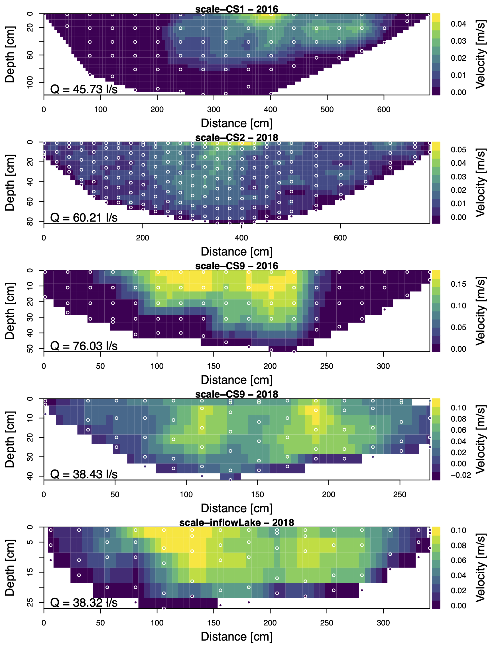
Figure 16 Water velocities at different cross-sections and years. White-circled points represent point-wise measurements made with an electromagnetic current profiler. The regular grid is produced by linear interpolation to a regular grid size resolution of 5 cm. The script to calculate the discharge (“/auxiliary/scripts”) allows to set different interpolation resolutions.

Uncertainty and errors

In the years 2016 and 2018, multiple measurements were conducted at different positions along the river within a same week. The derived discharge estimates differ by a factor of two (Fig. 16), while there was no indication in the field to expect such a difference. The measurement points had no systematic influence as the reversal of higher and lower estimates for the points near the inflow (“inflowLake”, “CS-1”, “CS-2”), and the points in the further downstream segment (“CS-9”) shows. From the presented differences between two points on the same river, the error is assumed to be at least of the magnitude, i.e. around 30 L s⁻¹. Uncertainties arising from the interpolation to a regular grid, especially when using large cell sizes, were estimated to be as high as 20 %.

4.3.6 Water stable isotopes – “istp”

Water samples were taken between 2013 and 2016 and analyzed for stable isotopes ¹⁸O, and ²H in at GEOPS laboratory in Paris-Saclay. The measurements were determined by cavity ring down laser absorption spectroscopy (CRDS, DLT-100 LWIA Los Gatos research; GEOPS-LSCE Panoply platform). The water isotope contents are reported in the conventional δ notation per mil (‰) as a deviation from the V-SMOW (Vienna Standard Mean Ocean Water) (Fig. 17). The accuracies are 1.5 ‰ for ²H and 0.2 ‰ for ¹⁸O (H₂O).

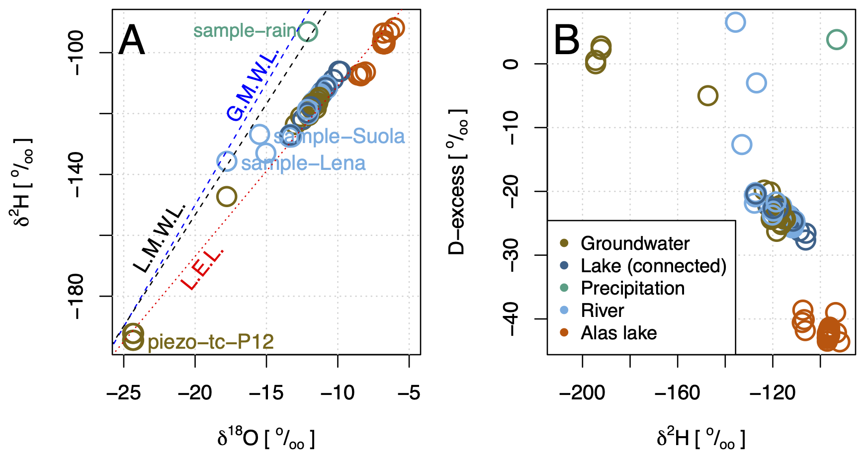
Figure 17 (A) Stable water isotope concentrations with respect to Vienna standard mean ocean water of water sources at the field site and two river samples from the Suola and Lena rivers, and (B) Deuterium excess values. Global meteoric water line (G.M.W.L.), local meteoric water line (L.M.W.L), and local evaporation line (L.E.L.) are adopted from Ichiyanagi et al. (2003).

Uncertainty and errors

No significant errors from sampling, storage, or transport were indetified. The results showed consistent estimates with no deviation from the meteoric water lines (Fig. 17).

4.3.7 Dissolved organic carbon – “DOC”

Data for dissolved organic carbon (DOC), dissolved oxygen saturation (DO), and other water chemistry parameters were measured in the region by Hughes-Allen et al. (2020) and Hughes-Allen et al. (2021). These data are available in a PANGAEA repository (Hughes-Allen et al., 2020). The present database includes these data in a homogenized way, where file and folder structure and descriptions have a matching format. The measurement points are included in the QGIS project with a label prefix “sample-HA”. Processing protocols and sampling strategy are described in detail in Hughes-Allen et al. (2021). DOC was determined using a Shimadzu TOC-L Total Organic Carbon Analyser series (SDN:L22::TOOL1760). The samples were filtered using baked glass fiber filters (Whatman GF/F, 0.7 µm), acidified to pH 2 with ultra-pure HCl and stored in baked glass vials (Hughes-Allen et al., 2020). DOC concentration was then measured in the TOC-5000A analyzer with a quantification limit of 1 mg L⁻¹, and an associated analytical uncertainty of ±0.1 mg L⁻¹ (Hughes-Allen et al., 2020). Reference material included ION-915 ([DOC] = 1.37 ± 0.41 mgC L⁻¹) and ION 96.4 ([DOC] = 4.64 ± 0.70 mgC L⁻¹) (Hughes-Allen et al., 2020). The exact sampling dates are not available in the original data repository (Hughes-Allen et al., 2020). Instead, only the seasons (Spring, Summer, Fall, Winter) were reported. This information is provided in a separate column in the homogenized CSV files. The different water source types are indicated in an additional column as lake (l), Alas or thermokarst lake (tl), river (r), or groundwater (g).

Uncertainty and errors

As for the isotope analysis, no significant errors or uncertainties outside the analytical uncertainty were identified. Lake and river samples were taken in distance of the immediate shorelines and no deviation from standard sampling protocols occurred, nor could we identify any suspicious data points within the analyses.

4.3.8 Dissolved oxygen saturation – “DO”

DO was measured alongside DOC by Hughes-Allen et al. (2021) using a YSI Pro DSS multi-parameter meter sensor. The relevant data in their original formatting can be obtained via: Hughes-Allen et al. (2020). As for DOC, the sample locations have the prefix “sample-HA”. The same additional columns as for DOC are provided in the data files (see Sect. 4.3.7).

Uncertainty and errors

As for conductivity and pH (see above), the YSI multi-parameter probe was calibrated at the start of each field mission, and could be calibrated daily using a calibrating cup. Multiple calibration sessions over the years have shown that the sensors, including the DO sensor, do not drift significantly.

4.4 Auxiliary measurements and data – “auxiliary”

4.4.1 UAV derived digital surface model (DSM) – “dsm”

Imagery of an UAV survey with two flights from 18 September 2021 using a DJI MavicPro 2 was used to create a digital surface model (DSM) and an orthomosaic image using Pix4D software. The UAV flight height was 120 m to obtain an image overlap of 70 % (front and sideways) with a total of 1062 images. No ground control points (GCPs) could be taken because the differential GPS was not operational. The images were hence calibrated without GCPs, and a 3D model was correctly constructed and georeferenced using only the positional data from the UAV's GNSS positioning system.

This resulted in an absolute horizontal accuracy of 1 to 2 m and an absolute vertical accuracy of 2 to 3 m. The obtained relative accuracy was 2 to 5 cm (horizontal), and 2 to 6 cm (vertical). The exported orthomosaic and DSM have a spatial resolution of 2.2 cm px⁻¹ and are provided in UTM zone 52N projection with WGS84 datum. Tree cover alongside the valley resulted in various elevation artifacts that render the use of the DSM for hydrological applications in these regions not useful. Therefore, two DSM masks for the GIS database in geopackage format were created manually and can be found in “auxiliary/geopackage”; the first is a cropping mask to remove any obvious artifacts, and a second one that crops out the majority of trees to facilitate any flow-related analysis close to the river.

Uncertainty and errors

Despite the reported high relative vertical accuracy, the DSM has a significant problem with elevation gradients. While there is an overall decrease downstream in elevation, the middle section is slightly higher than the stream section close to the upstream lake. This would prevent any water flow downstream – this is true also for the DSM without trees using the manually created DSM masks to remove artifacts and trees. Apart from the lack of GCPs, another reason for this may be due to the uncertainty in GPS positions of the drone between two flights or because it is a DSM that includes the vegetation such as tall grass. The error in vertical elevation by investigating the river channel was estimated to be around 2 m. The user is advised to modify the DSM for hydrological applications that require a continuous gradient from the upstream to the downstream lake. The lateral gradients are much stronger and allow direct usage of the DSM without modifications.

4.4.2 Geographic positions – “gps”

Positions of measurement locations were recorded using one or multiple of the three devices: (1) Leica Viva Uno 10 (GPS + GLONASS) differential GPS (dGPS) system, (2) a Ural Optical and Mechanical Plant 3T5KP Theodolite with 2 (5) arcsec horizontal (vertical) resolution, (3) GARMIN handheld GPS with around 10 m accuracy.

The Leica Viva Uno 10 was operated in differential RTK mode using a temporary base station that was established through multi-hour static observations (between 1 and 3 h) and subsequently used for short-baseline RTK measurements (100 m to 3 km). Under such conditions, typical absolute positioning accuracy was expected to be within few centimeters to decimeters (5 to 20 cm).

However, as base stations were re-established independently for different campaigns and cross-sections, small systematic offsets between campaigns are expected. Investigation of the positions of different years for the same locations showed, however, differences of up to 1 m. For the different campaigns, additional information was unavailable about which positions were more reliable, or about possible reasons for this offset. In order to coherently homogenize all measurement positions with the landscape features (Sect. 4.4.1), the DSM (as is) was used as the basis for homogenization and to maximize the usefulness of the database. Hence, the measurement points were manually aligned within the GIS database with identifiable landscape features. For this, the points were aligned to known fix points in the orthomosaic photo, like the river shoreline or forest-meadow boundary. In case a user requires more accurately or differently aligned points, it is possible to adjust the positions of features in the GIS project and extract the resulting adjusted positions using a provided Python script (Sect. 4.4.3).

Uncertainty and errors

The expected uncertainties from using the dGPS with re-initializations for different measurement locations and different years were significantly lower than the observed differences identified between different years (up to 1 m). We do not have the means to assess the sources of error. By adjusting points manually to align with identified points in the orthomosaic, we additionally introduced a maximal horizontal error of around 3 m. However, based on the reasoning to prioritize a coherent alignment of points with landscape features in the DSM, the relative error was assumed to be < 1 m.

4.4.3 Processing scripts – “scripts”

The database provides four categories of scripts for (i) “plotting”, (ii) extraction and management of “coordinates”, (iii) data comparison and gap filling via “regression” analyses, and (iv) “discharge” calculation. The scripts to produce the figures within this manuscript, conduct the regression analysis, and to calculate discharge from water velocity measurements are provided in the R language, and scripts for the extraction of coordinates from the vector files are written in Python.

Plotting

The plotting functions used to produce the figures in this manuscript showcase the file-specific loading and processing routines for any of the CSV files in the database. The sub-folder structure of the plotting functions follows the organization of the main database by each individual variable. Additionally, one script (“/overview”) extracts all meta-information of all CSV files in the database for the creation of the overview figure (Fig. 3).

Coordinates

The coordinates extraction script is designed to achieve an independence of the GIS files and analyses of measurements in a geo-spatial context. As described in Sects. 3.2 and 4.4.2, point measurements inherit inaccuracies resulting from point registrations with handheld GPS, or re-initiated dGPS receivers (Sect. 4.4.2). The users can check within the ortho-mosaic and derived DSM the positions of points and make adjustments if needed within a GIS. The script then allows for fast extraction of so-adjusted coordinates for further processing (e.g. plotting with spatial referencing). The script automatically creates a CSV file named coordinates_<YYYY-MM-DD>.csv, where <YYYY-MM-DD> is the date of creation as year, month, and day. The file is created in the main database folder and includes the coordinates as latitude and longitude, Easting and Northing in UTM zone 52N coordinates, and the point measurement labels. The point labels are referenced in each CSV measurement file, either directly within the file name for single point measurements, or as indices in case of multiple point measurements.

Discharge

The discharge was calculated by first interpolating the existing arbitrarily distributed point-wise measurements of stream velocities over a river cross-section onto a regular 2D grid using the R library “akima” (Akima and Gebhardt, 2022). The grid resolution can be defined by the user. The interpolated values are finally summed up and its units converted to L s⁻¹.

Regression

As highlighted in Sects. 4.3.4 and 4.2.1, atmospheric pressure and temperature were not continuously available. In order to use data from the nearest meteorological station Yakutsk (WMO ID = 24 959, 103 m a.s.l.), the scripts in the sub-folders “Diver” and “TAIR” were used to perform a regression analysis for the overlapping periods. From the obtained linear models, air pressure, and air temperature were reconstructed for the data periods with no local measurements. The resulting data files are contained within the respective folders under “regression”.

4.4.4 Vector files for GIS – “geopackage”

Each measurement location is stored in a point or polygon vector file in GeoPackage format under “auxiliary/geopackage”. The naming of GeoPackage files and contained points follows the main instrument or measurement technique applied to obtain the measurement. This means that, e.g., an infiltration test in a soil pit is not separately listed as infiltration point, but instead the location of the soil pit is provided. The relevant location names are explicitly stated in the CSV files. Polygon vector files are available for most of the soil pits. Each GeoPackage file has, in addition to the location, attributes about start and end date of the measurements conducted at an individual position, and a boolean flag whether the exact date of the measurements was known. This flag was required as some data (DO, DOC) were only associated with a season, and some measurements were conducted within a time window over multiple days.

5 Data availability

All data presented in this manuscript are available in a zenodo database under CC 4.0 license (https://doi.org/10.5281/zenodo.14619854, Pohl et al., 2025). The raw data of UAV imagery that were used to derive the DSM and orthomosaic photo are available upon request from Antoine Séjourné.

6 Code availability

The code to process the data and produce the figures are included in the zenodo database under CC 4.0 license (https://doi.org/10.5281/zenodo.14619854; Pohl et al., 2025).

7 Conclusions

This database shall serve specifically the development of thermo-(hydrological) modeling code, in a region where changes to permafrost under climate change are expected but data are sparse. With a focus on ground temperatures at different depths and by providing various topsoil temperatures, the difficult-to-account-for heat transfer through snow layers is avoided. Shallow soil temperatures from various landscape units with different expositions and vegetation allow for the analysis of air-ground temperature relationships and explore the inherent small-scale variability this has on heat transfer. Ultimately, this shall help improving the code within large-scale land surface models that are required to obtain more reliable future climate estimates. The rich set of supporting data on ground physical properties and water chemistry will allow setting much-needed boundary conditions and validation of modeling exercises.

Appendix A: Data correction and validation with third-party datasets

The following shows correlation analyses to reconstruct incomplete atmospheric pressure, and air temperature data using continuous time-series from the meteorological station in Yakutsk (WMO ID = 24959, 103 m a.s.l.). The data were homogenized using simple linear regression. Obtained relationships are directly shown within the figures. Furthermore, a comparison of soil water content obtained from different TDR probes against laboratory estimates are shown.

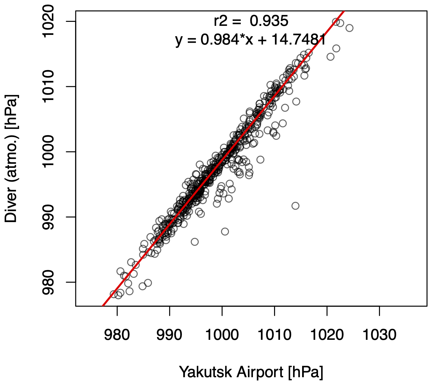
Figure A1 Comparison of atmospheric pressure measured since 2017 in the Syrdakh village and Yakutsk meteorological station (WMO ID = 24959). The atmospheric pressure from Yakutsk was used then to correct the water pressure sensors for the influence of atmospheric pressure variability.

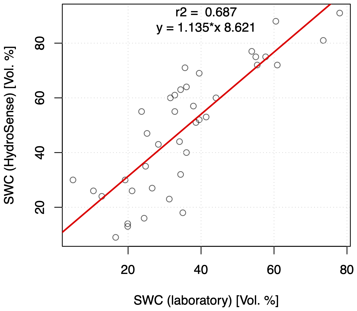
Figure A2 Comparison between soil water content (SWC) determined in the laboratory (LSCE or MPI) and in situ using the HydroSense instruments.

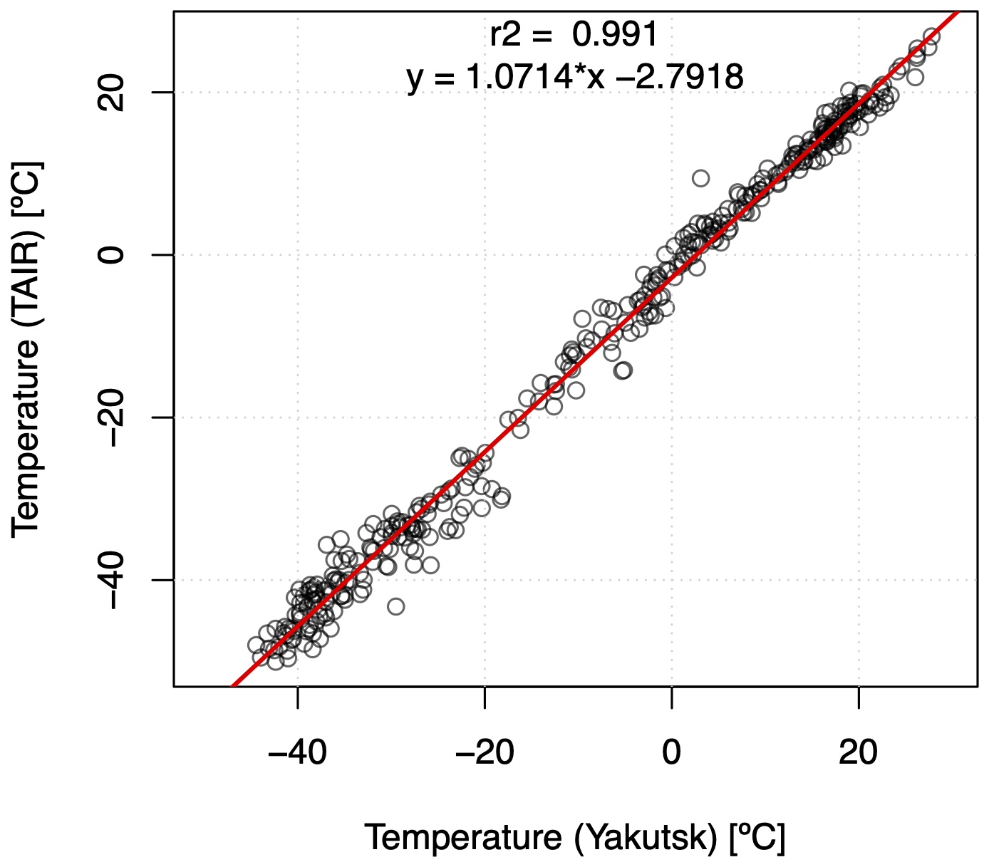
Figure A3 Comparison between meteorological station Yakutsk (WMO ID = 24959) and T&D RTR-502 (TAIR) temperatures.

Appendix B: File header examples

The following section shows an example of header information within the two main data types: time-series and tests (Table B1).

Table B1 Example of CSV file metadata with 22 lines of generalized categories (left column). Two examples, one for a soil temperature time-series of a TB (middle), and one for groundwater depth measurements at various points (right column).

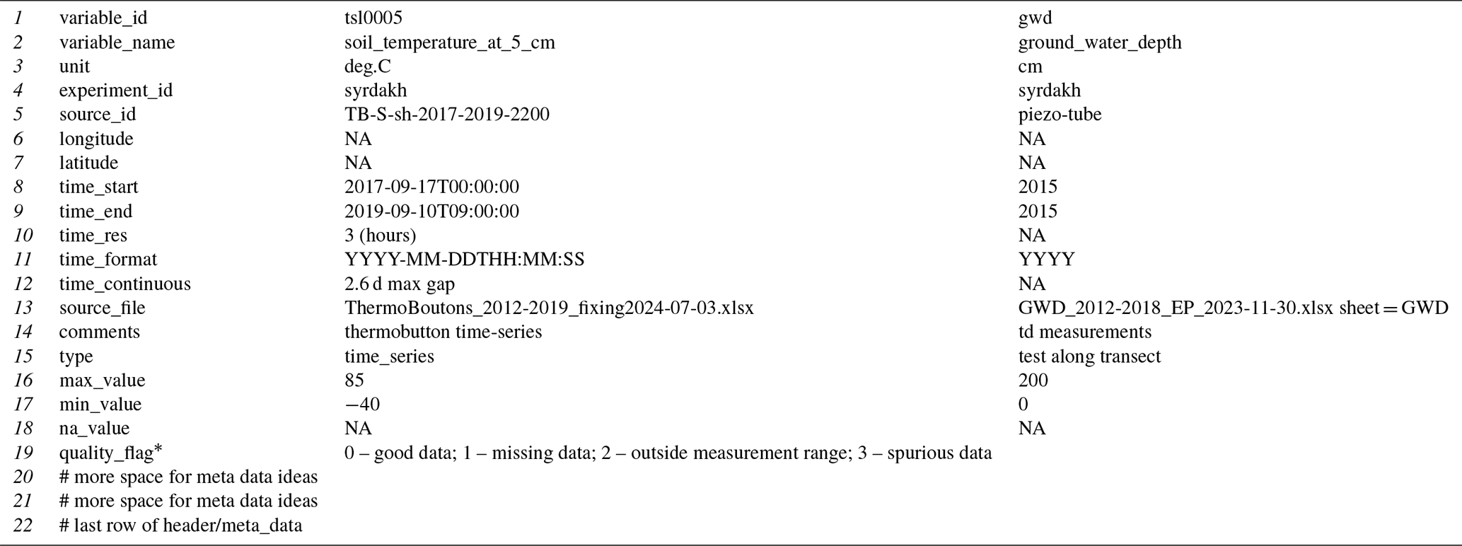
^* Quality flag entry only for time-series data.
NA: not available.

Appendix C: ERT and GPR data

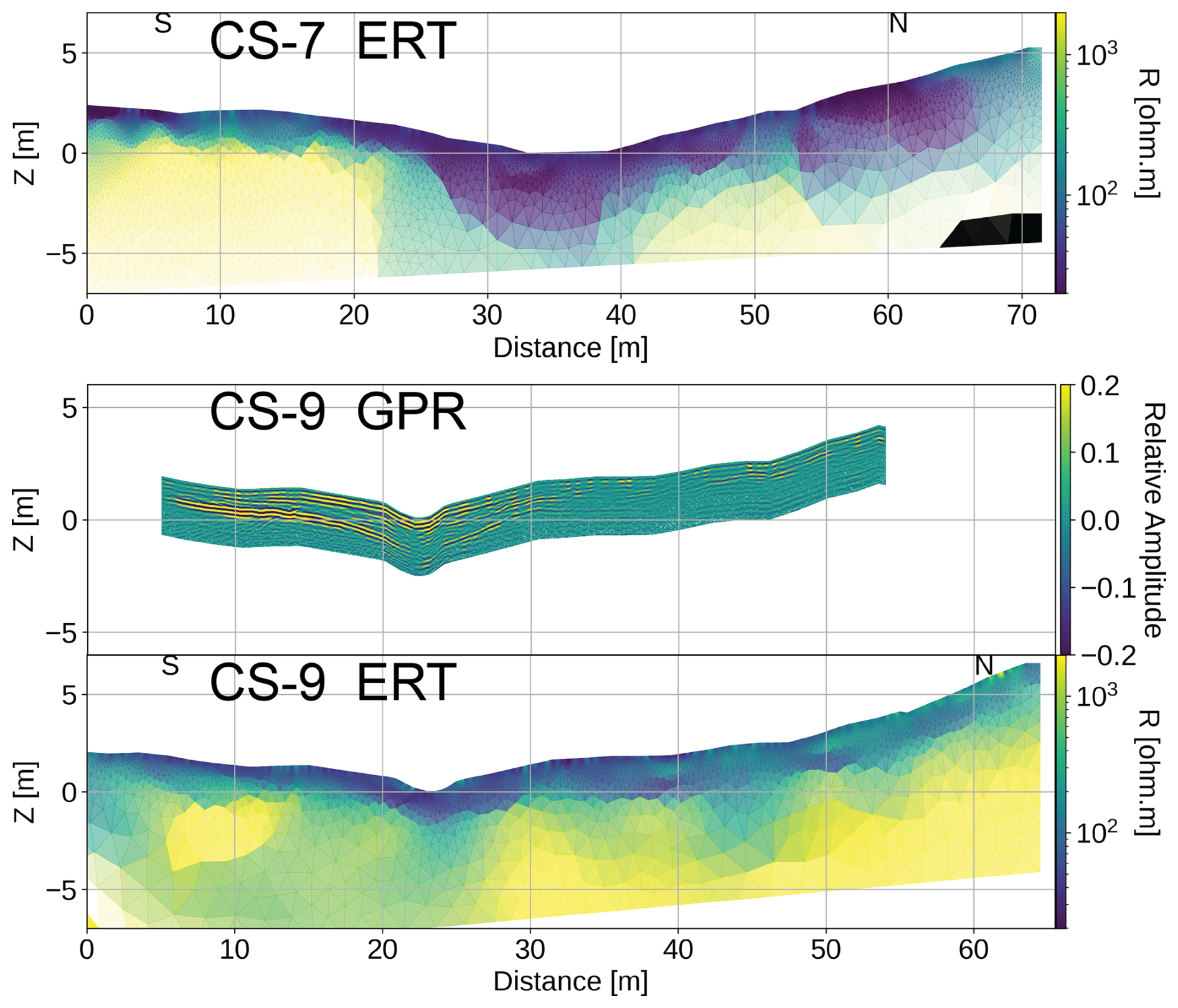
Figure C1 Geophysical measurements at CS-7 (ERT) and CS-9 (ERT + GPR) from Léger et al. (2023). For details on data processing see their publication.

Appendix D: Photos of instruments and locations

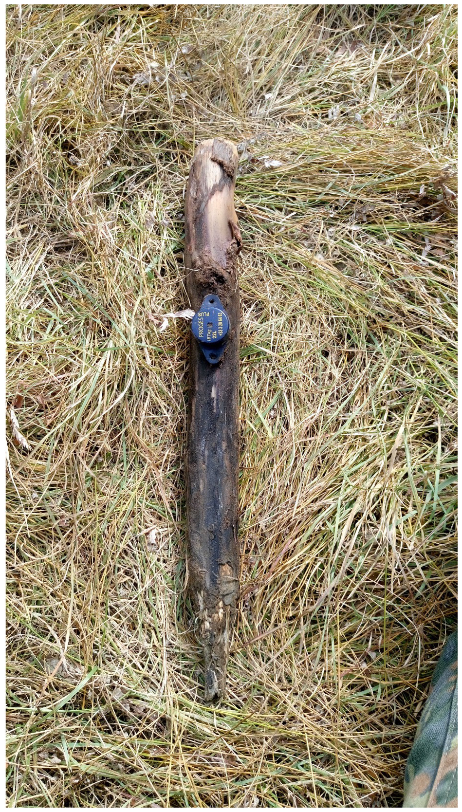
Figure D1 Proges Plus Thermo Buttons 22L (TB) attached on wooden peg. Installation by pushing or hammering into the soil to a depth of approximately 5 cm.

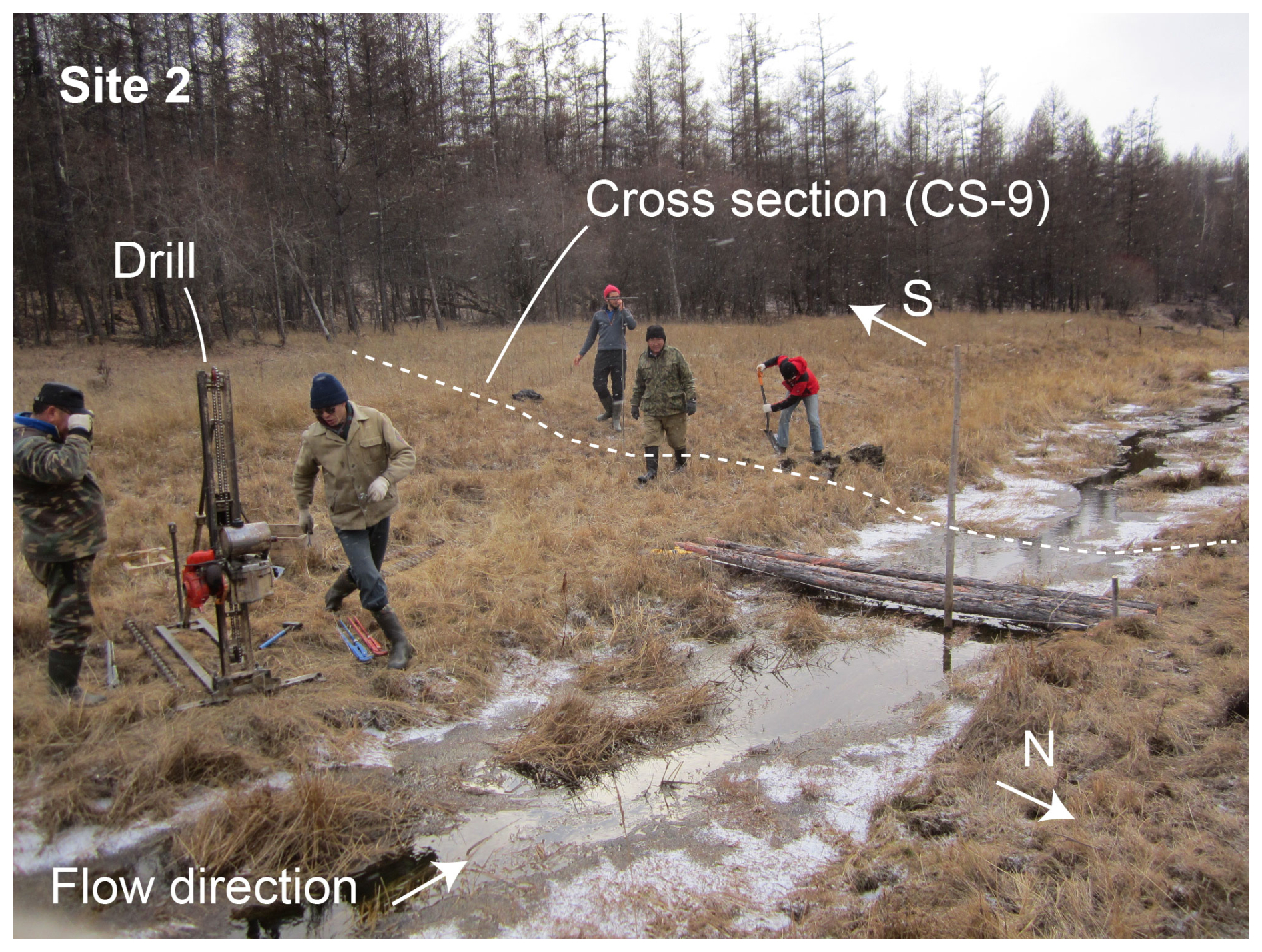
Figure D2 Installation of HOBO thermistor chains, and piezometer tubes at Site 2 (CS-9) with a petrol powered standing drill.

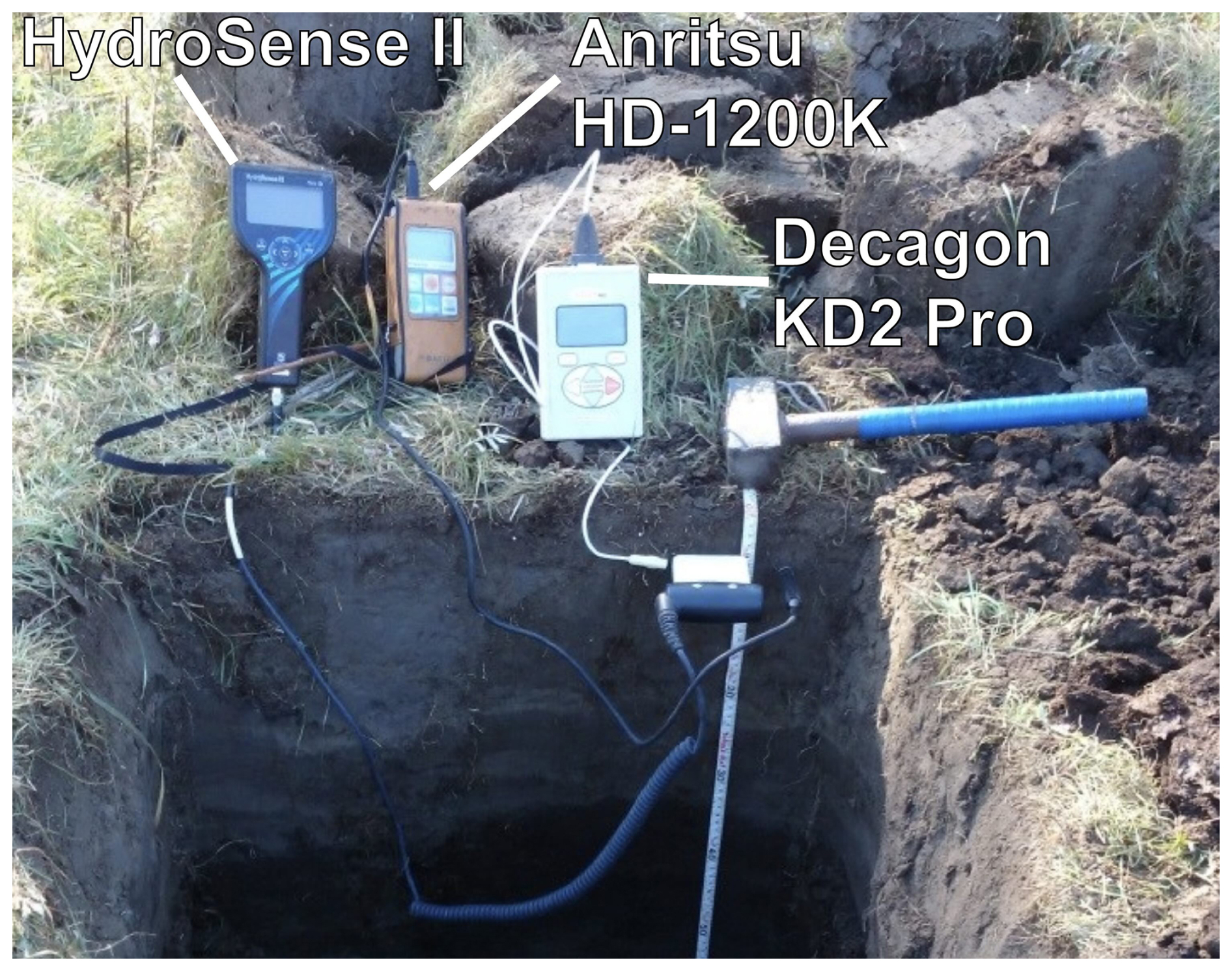
Figure D3 Thermal instruments of Anritsu (thermometer) and a Decagon Devices KD2 Pro installed in a soil pit. Volumetric water content was determined alongside using a Campbell HydroSense I or II (here II).

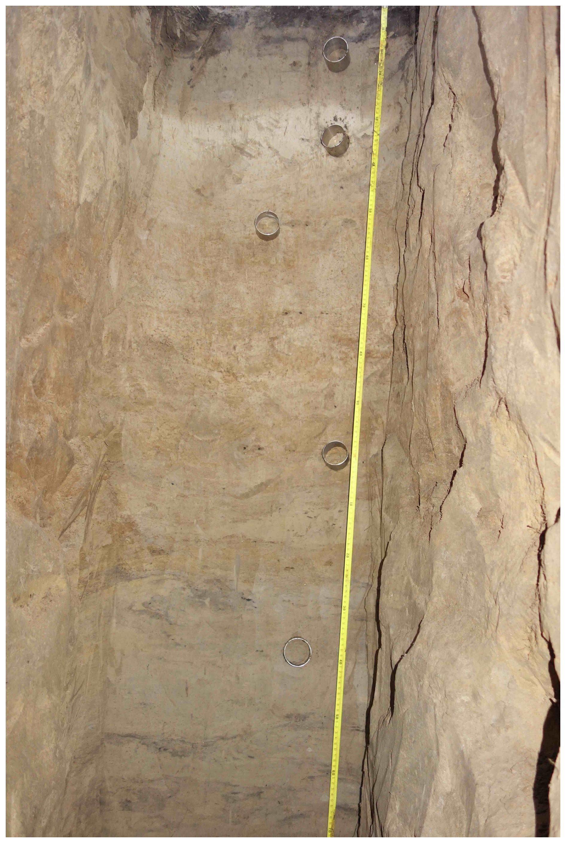
Figure D4 Soil pit “pit-2017-RB-2” with metal cylinders for soil soil sampling. Old radiocarbon ages of topsoil (upper two sampling cylinders) were determined while subsequent samples show older ages with depth.

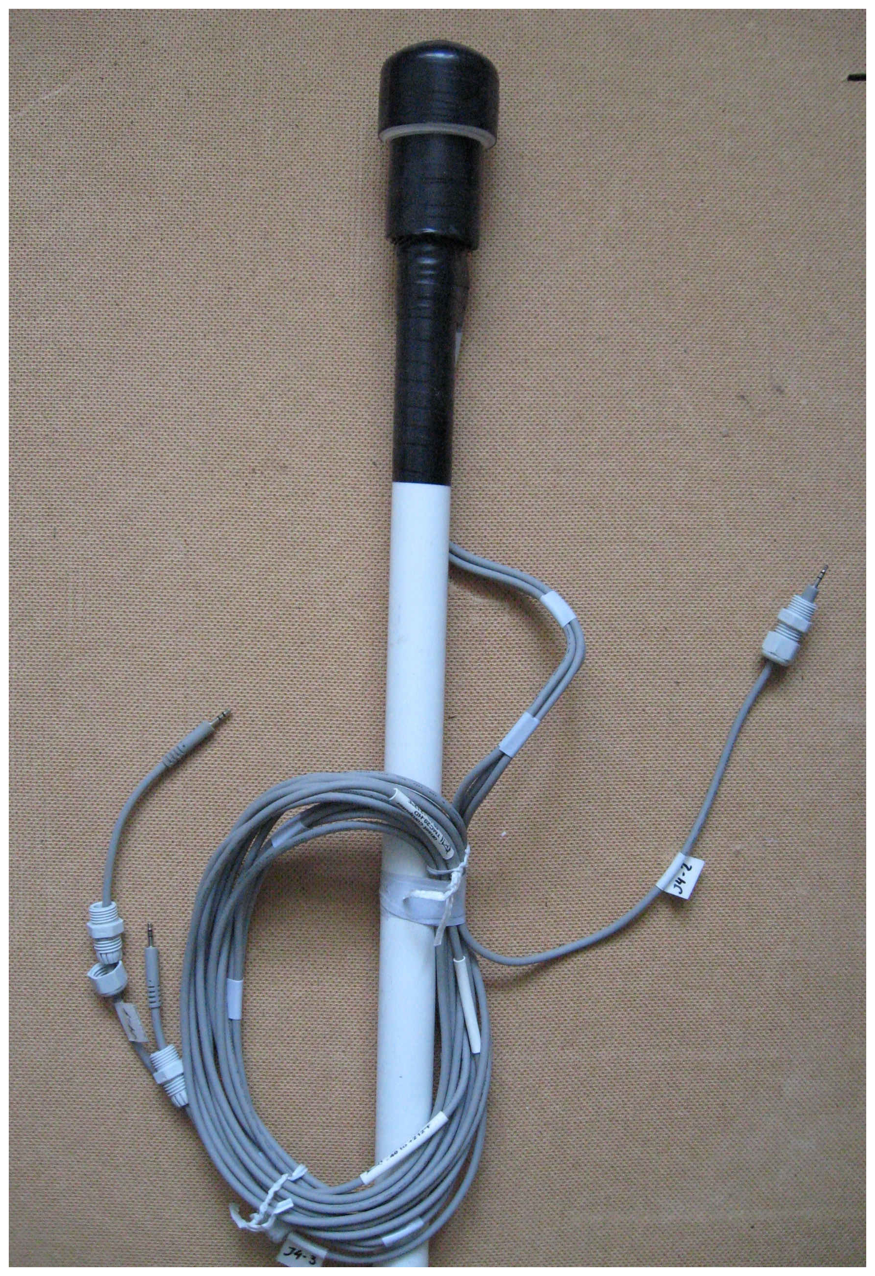
Figure D5 HOBO thermistor chain construction before installation in borehole. Construction consists of four thermistors that wired and held in place at specific and predefined depths within a PVC tube of 50 mm diameter that is filled with dry sand before installation.

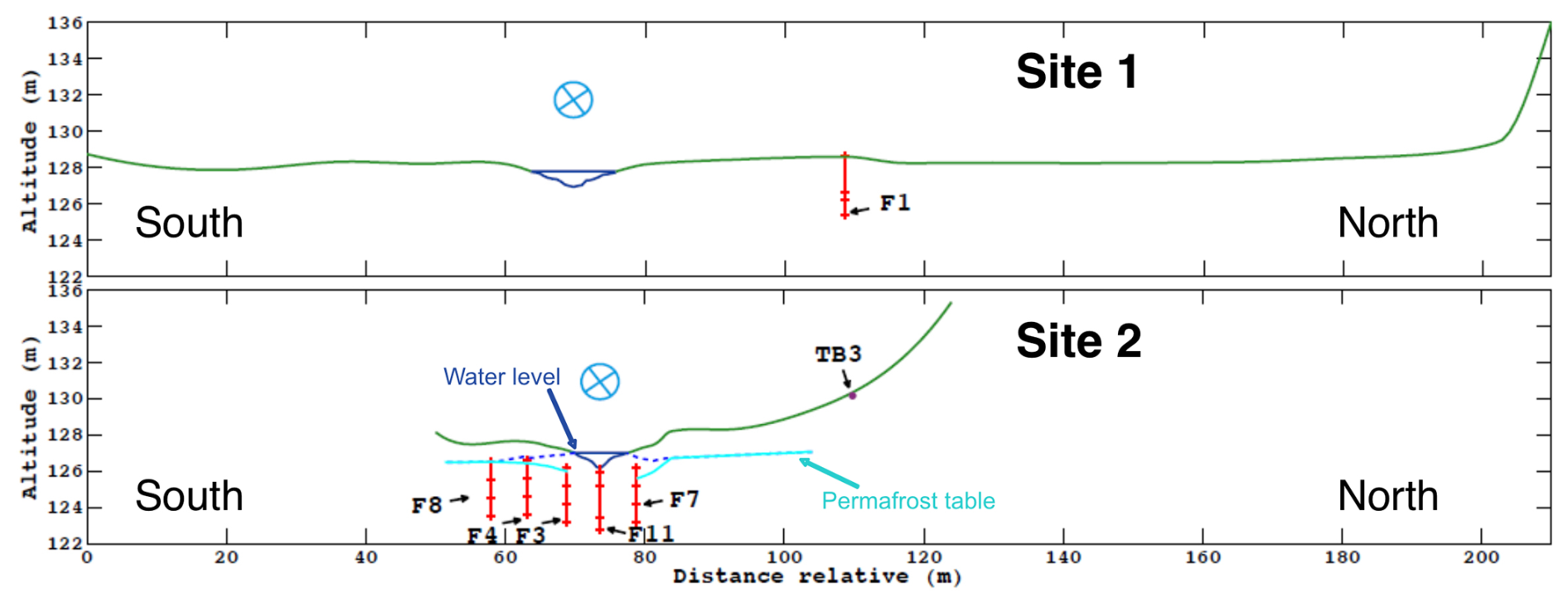
Figure D6 Schematic view of HOBO thermistor chain installation at the two cross sections of Site 1 and Site 2.