Reconstruction of δ¹³C_DIC in the Atlantic Ocean: a probabilistic machine learning approach for filling historical data gaps

Stable carbon isotope composition of marine dissolved inorganic carbon (DIC), δ¹³C_DIC, is a valuable tracer for oceanic carbon cycling. However, its observational coverage remains much sparser than that of DIC and other physical or biogeochemical variables, limiting its full potential. Here, we reconstruct δ¹³C_DIC in the Atlantic Ocean using a probabilistic machine learning framework, Gaussian Process Regression (GPR). We compiled data from 51 historical cruises, including a high-resolution 2023 A16N transect, and applied secondary quality control via crossover analysis, retaining 37 cruises for model training, validation, and testing. The trained GPR model achieved an average bias of −0.007 ± 0.082 ‰ and an overall uncertainty of 0.11 ‰, arising from measurement (0.07 ‰), mapping (0.08 ‰), and input-variable (0.009 ‰) errors. To address validation limitations related to sparse observations, we further supplemented this work with numerical model-based validation (Claret et al., 2021), confirming the GPR model's robustness in δ¹³C_DIC reconstruction. Using the GLODAPv2.2023 Atlantic dataset as predictors, the reconstruction expanded the number of acceptable δ¹³C_DIC samples by a factor of 7.65, from 8941 to 68 435 across the Atlantic basins. The resulting dataset markedly improves the spatial resolution in longitude, latitude, and depth, and provides enhanced temporal continuity over the past four decades, offering great advantages in decadal trend assessment. Compared to the sparse original measurements, the reconstruction also reduces spatial discontinuities and reveals finer vertical structures consistent with other high-resolution biogeochemical observations. Additionally, the validated GPR framework was applied to the GLODAPv2 1° × 1° global interior ocean mapped climatology (Lauvset et al., 2016), producing a climatological gridded 3D δ¹³C_DIC dataset for the Atlantic Ocean. These reconstructed δ¹³C_DIC datasets provide new opportunities to resolve regional carbon cycle dynamics, validate Earth system models, refine estimates of oceanic carbon uptake on at least decadal timescales, and extend climate reanalysis records. The reconstructed δ¹³C_DIC data, quality-controlled observational data from 51 cruises, and gridded δ¹³C_DIC product are available at https://doi.org/10.5281/zenodo.18481145 (Gao et al., 2025).

1 Introduction

The stable carbon isotope ratio has been widely applied as a tracer in marine carbon research, providing valuable insights into various processes within the oceanic carbon system. It is expressed via the standard delta notation: δ¹³C = ((¹³C $/$ ¹²C)${}_{\mathrm{sample}}/{(}^{\mathrm{13}}$C $/$ ¹²C${)}_{\mathrm{standard}}-\mathrm{1})\times {\mathrm{10}}^{\mathrm{3}}$, referenced against the international standard, the Vienna Pee Dee Belemnite (V-PDB) fossil. Specifically, the δ¹³C of dissolved inorganic carbon (DIC), denoted as δ¹³C_DIC (expressed in per mil, ‰), has proven instrumental in studies encompassing estimating rates of biological production in surface ocean mixed layer (Quay et al., 2003, 2009; Yang et al., 2019), quantifying anthropogenic carbon inputs and accumulations in ocean basins (Quay et al., 1992, 2003, 2007, 2017; Körtzinger et al., 2003; Olsen and Ninnemann, 2010; Racapé et al., 2013), and validating earth system models (Sonnerup and Quay, 2012; Schmittner et al., 2013; Liu et al., 2021; Claret et al., 2021), making it an indispensable parameter in understanding the complexities of the marine carbon cycle.

Measurements of δ¹³C_DIC in the ocean trace their roots to the mid-20th century, with significant advancements occurring in the 1970s and 1980s due to the development of more precise mass spectrometry techniques. A pivotal moment in marine isotope research came with Kroopnick's comprehensive analyses of δ¹³C_DIC distribution in the Atlantic Ocean (Kroopnick, 1980a) and globally (Kroopnick, 1985), which provided critical insights into isotopic patterns across the oceans. Over subsequent decades, observational δ¹³C_DIC data and their biogeochemical interpretation continue to increase (Gruber et al., 1999; Quay et al., 2003, 2017; Schmittner et al., 2013). The creation of databases such as Global Ocean Data Analysis Project (GLODAP) further enhanced access to δ¹³C_DIC data and other carbon-related parameters (Olsen et al., 2016). However, unlike other carbon datasets such as DIC and total alkalinity (TA), δ¹³C_DIC lacked secondary quality control until Becker et al. (2016) introduced an internally consistent δ¹³C_DIC dataset for the North Atlantic, marking a significant step in addressing biases and improving data reliability. But still, unlike other carbon datasets, δ¹³C_DIC lacks necessary sufficiently high spatial resolution for it to be effective in ocean carbon cycle research and as a tracer for anthropogenic carbon accumulation in the ocean.

Traditionally, δ¹³C_DIC data have been acquired by preserving and transporting seawater samples to shore-based laboratories for analysis via Isotope Ratio Mass Spectrometry (IRMS). Although the IRMS approach is highly precise and accurate, it is labor-intensive and unsuitable for at-sea analysis, and incapable of measuring precise DIC concentrations concurrently. These limitations have significantly restricted the collection of δ¹³C_DIC data, impeding efforts to characterize spatiotemporal variabilities and long-term trends of δ¹³C_DIC. For example, in the Atlantic Ocean, only 6820 δ¹³C_DIC measurements were collected across 32 cruises over 40 years, averaging just 213 samples per cruise (Becker et al., 2016). Specifically, along the A16N transect, approximately 500 samples were collected during the 1993 and 2013 cruises and only 38 surface water samples were collected during the 2003 cruise for land-based δ¹³C_DIC analysis, showing a stark contrast to the fact that about 3000 DIC samples were analysed at sea per cruise. To overcome this severe bottleneck, the Cai Lab has developed a precise, rapid, and sea-going suitable δ¹³C_DIC analytical method with a precision of better than ±0.05 ‰ based on the Cavity Ring-Down Spectroscopy (CRDS) stable carbon isotope analyzer, G2131-i (Su et al., 2019; Deng et al., 2022; Sun et al., 2024, 2025). This method has been extensively tested during several recent observations and studies. During a long (58 d) ocean cruise along A16N in 2023, approximately 3500 δ¹³C_DIC samples were collected, with ∼ 3000 samples analysed at sea, alongside DIC observations. This progress has significantly surpassed the historical A16N datasets (Sun et al., 2025).

Despite extensive field data collection efforts, observations of δ¹³C_DIC remain sparse compared to other inorganic carbon chemistry variables (e.g., DIC and TA). The distribution and variations of inorganic carbon chemistry within water masses are governed by both the source-water properties and physical and biogeochemical processes, resulting in region-specific stoichiometric relationships among inorganic carbon variables. These relationships are typically nonlinear and exhibit spatial and temporal variability, making it challenging to determine general distribution patterns. In recent decades, advancements in machine learning techniques coupled with accumulated observational data have facilitated numerous studies that interpolate inorganic carbon chemistry variables, particularly the partial pressure of CO₂ (pCO₂) due to its relatively high spatial coverage, from satellite data and reanalysis products (e.g., Landschützer et al., 2016; Gregor and Gruber, 2021; Roobært et al., 2024; Wu et al., 2025). These methodological developments present a promising opportunity to investigate the potential for deriving δ¹³C_DIC data from more abundantly measured variables.

Given the limited and fragmented δ¹³C_DIC dataset compared to other parameters such as DIC, and to fully utilize the δ¹³C_DIC tracer approach for quantifying anthropogenic CO₂ uptake by the ocean (Quay et al., 2017), the rate of ocean biological production (Esposito et al., 2019; Quay et al., 2009, 2020; Quay, 2023), and carbon cycling across the land-ocean interface (Alling et al., 2012; Kwon et al., 2021; Samanta et al., 2015), this study aims to reconstruct a high-resolution δ¹³C_DIC dataset for the Atlantic Ocean using Gaussian Process Regression (GPR), a probabilistic machine-learning approach capable of capturing nonlinear relationships and spatial-temporal variability. This reconstruction integrates historical δ¹³C_DIC observations in the Atlantic Ocean with new high-resolution data collected along the A16N transect in 2023 (Sun et al., 2025), the GLODAPv2 1°×1° global interior ocean mapped climatology (Lauvset et al., 2016), and the product of GLODAPv2.2023 (Lauvset et al., 2024). The final product consists of three components with comprehensive uncertainty analysis: (1) a quality-controlled δ¹³C_DIC observational dataset compiled from 51 cruises with a crossover analysis using standardized protocols, and (2) a machine learning-reconstructed δ¹³C_DIC dataset derived from other inorganic carbon chemistry variables, (3) a climatological 1°×1° gridded three-dimensional δ¹³C_DIC dataset for the Atlantic Ocean produced by applying the validated GPR framework to the GLODAPv2 1°×1° global interior ocean mapped climatology. The structure of this study is as follows: Sect. 2 describes the datasets used, the secondary quality control of δ¹³C_DIC, and the methodology for reconstructing the δ¹³C_DIC dataset. Section 3 evaluates the accuracy, performance, and applicability of the reconstructed δ¹³C_DIC dataset in resolving its spatial and temporal distribution. Section 4 presents the conclusions. Sections 5 and 6 provide access the dataset, the codes used for its generation, and the figures presented in this study. The Appendix provides additional evaluation and validation by applying the same GPR approach to numerical model outputs.

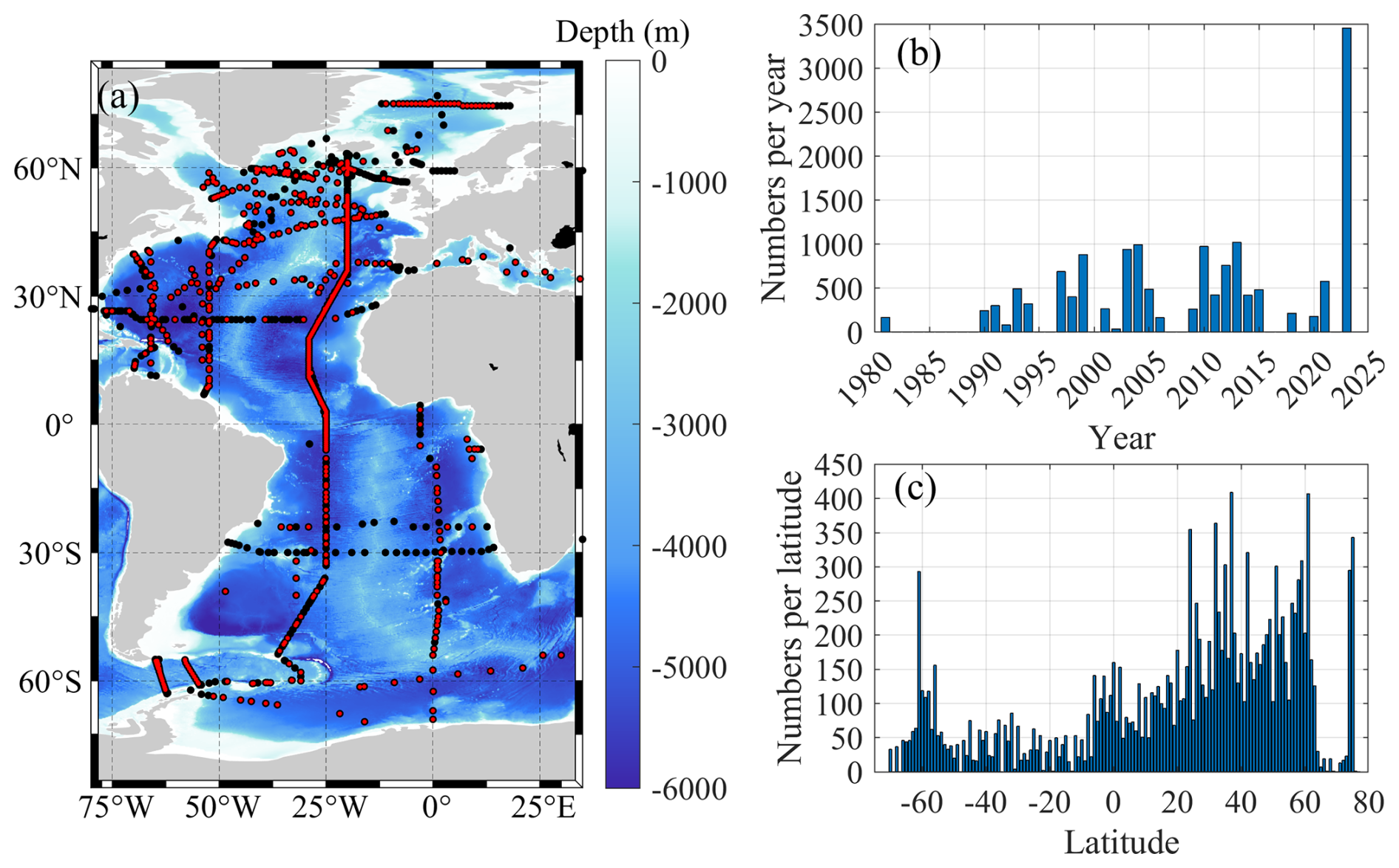
Figure 1 Overview of the collected δ¹³C_DIC data. (a) Map of all stations with δ¹³C_DIC data in the Atlantic Ocean, with stations containing samples deeper than 2000 m highlighted in red. (b) Temporal distribution of δ¹³C_DIC data, organized by year of collection. (c) Total number of δ¹³C_DIC samples aggregated by each degree of latitude.

2 Data and Methods

2.1 Data collection

2.1.1 Historical δ¹³C_DIC Data Collection

In the Atlantic Ocean, δ¹³C_DIC data were compiled from several international research initiatives, including GLODAP, Ocean Carbon and Acidification Data System (OCADS), Climate and Ocean Variability, Predictability, and Change (CLIVAR), Carbon Hydrographic Data Office (CCHDO) and the internally consistent dataset of δ¹³C_DIC in the North Atlantic Ocean (NAC13v1, Becker et al., 2016). Notably, most cruises in the final compiled dataset are sourced from GLODAP. Cruises from the other aforementioned databases were only included to supplement those not covered by GLODAP, and no duplicate cruises were counted to ensure each unique cruise is represented exactly once. From the original dataset published by Becker et al. (2016), we excluded four cruises: 35TH20060521, 74JC20120601, 74DI20140606, and OMEX1NA, due to missing essential corresponding parameters, i.e., variables used for model training. The remaining cruises, including those from other sources and the 28 cruises retained from Becker et al. (2016), comprise a total of 51 cruises, covering 369 stations and 15 225 δ¹³C_DIC samples (Fig. 1 and Table 1). To ensure internal consistency, samples from depths greater than 2000 m were selected for crossover analysis. Specifically, deep waters below 2000 m in the South Atlantic Ocean are most likely not impacted by anthropogenic carbon (i.e., Gao et al., 2022, 2024), supporting this threshold. In contrast, North Atlantic Deep Water (NADW) formation may drive small but measurable decadal anthropogenic carbon changes even below 2000 m. However, Becker et al. (2016) showed that restricting analysis to depths > 2000 m effectively reduces cruise offset variability in variable North Atlantic regions (e.g., Labrador Sea, Nordic Seas), further validating our 2000 m threshold for the Atlantic. This criterion resulted in 3772 samples from 305 stations deeper than 2000 m (highlighted as red points in Fig. 1a). The temporal and latitudinal distributions of the δ¹³C_DIC data are illustrated in Fig. 1b and c, respectively. These datasets span from 1981 to 2023, with the most comprehensive annual δ¹³C_DIC sampling occurring along A16N in 2023 (Fig. 1b). However, the sampling is spatially and temporally uneven, that is, data are sparse in certain years and latitudes, which underscores the need for an approach capable of generating robust predictions and uncertainty estimates in poorly sampled regions, such as the GPR method applied in this study. In particular, the majority of samples are concentrated in the North Atlantic, particularly between latitudes 25 and 60° N (Fig. 1c).

Table 1 Information about Cruises that contains δ¹³C_DIC, and adjustment for each cruise.

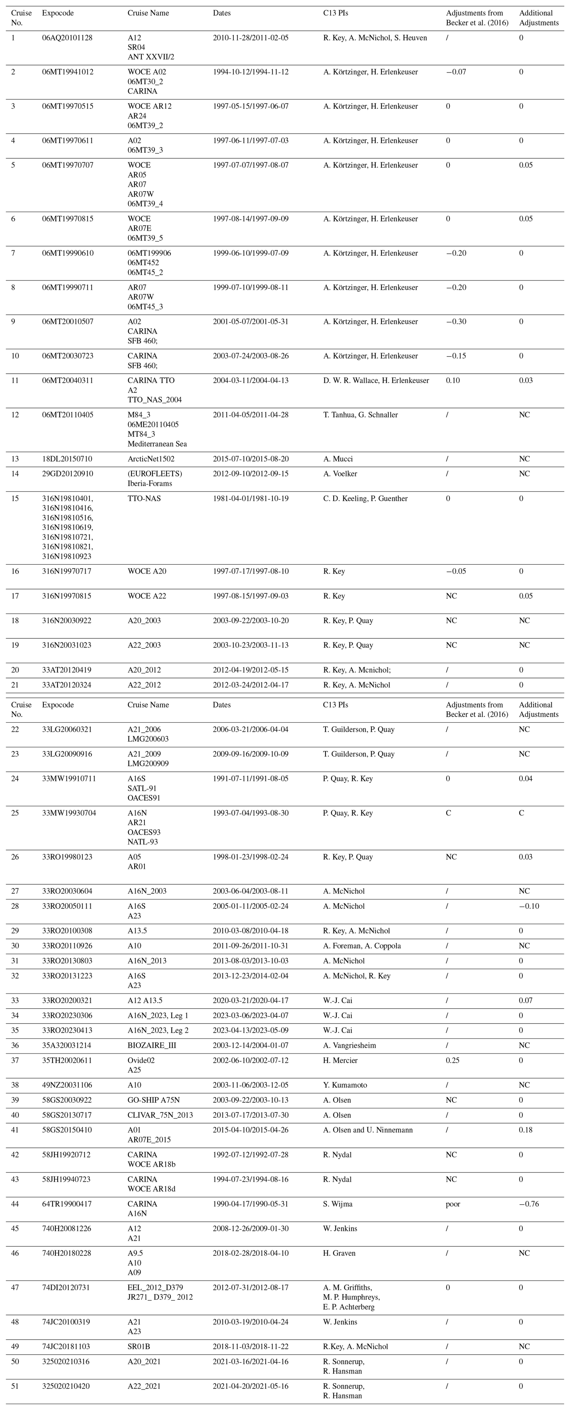
Note: NC denotes cruises that were not considered for the adjustment due to the absence of statistically significant crossovers. The core cruise, identified as the reference, is marked with a “C”.

2.1.2 δ¹³C_DIC Data Collection Along A16N in 2023

The A16N cruise in 2023 achieved extensive collection and high-resolution analysis of δ¹³C_DIC and DIC datasets over two legs using onboard analytical techniques. Samples were collected from CTD rosette bottles into 250 mL borosilicate glass bottles following PICES best practices, preserved with HgCl₂ to prevent biological activity, and sealed to prevent gas exchange. Analytical measurements were conducted onboard using two coupled systems comprising a CO₂ extraction device (AS-D1 δ¹³C_DIC Analyzer) and a CRDS (Picarro G2131-i), which simultaneously measured DIC concentrations and δ¹³C_DIC values with high precision. Quality control measures included frequent calibration using Certified Reference Materials (CRMs) and in-house standards verified by IRMS, ensuring high data reliability with deviations mostly within ±0.03 ‰ for δ¹³C_DIC (Sun et al., 2025).

2.2 Standardized Protocols for Crossover analysis

Secondary quality control of δ¹³C_DIC data through crossover analysis ensures consistency across multi-cruise datasets (Becker et al., 2016; Tanhua et al., 2010; Lauvset and Tanhua, 2015). The analysis involves compiling data from overlapping regions, identifying crossover points within 222 km, and comparing δ¹³C_DIC profiles in deep waters (> 2000 m) where variability is minimal. Profiles are interpolated to standard depths or density. In this study, we adopted the density-based interpolation: standard sigma4 surfaces (potential density referenced to 4000 m) are generated at 0.05-unit intervals, covering all observed densities, based on the interpolated density profile of the deepest station, following the workflows presented in Lauvset and Tanhua (2015). Mean offsets between overlapping profiles at the selected standard densities are calculated. Detailed workflows were. Systematic biases are identified using least squares minimization, and adjustments are proposed to align datasets without erasing real temporal or spatial trends. Adjustments are validated against known regional patterns and applied only if they reduce discrepancies to within the measurement uncertainty. All steps and corrections are documented to ensure transparency, resulting in reliable δ¹³C_DIC datasets for carbon cycle analysis. Building on the NAC13v1 dataset provided by Becker et al. (2016), we propose additional adjustment recommendations for these cruises (Table 1). Given that cruise 64TR19900417 crossovers with cruise 33MW19930704, 06MT20040311, 33RO20130803, 33RO20230413, showing a very high mean offset and standard deviation −0.76 ± 0.23 ‰, and its δ¹³C_DIC data is marked as NaN (missing values) in the NAC13v1 dataset, it is excluded from our analysis. After applying additional adjustments, the δ¹³C_DIC data for the remaining 37 cruises exhibit high internal consistency. These 37 cruises do not include 13 cruises without deep-water crossover stations (marked as NC in the last column “Additional Adjustments” of Table 1) and cruise 64TR19900417, which were excluded to ensure data reliability as their uncertainties cannot be objectively quantified. Collectively, these excluded cruises accounted for less than 3 % of total δ¹³C_DIC measurements. The internal accuracy of the adjusted δ¹³C_DIC is determined to be −4.15 × 10⁻⁵ ‰ based on the calculation from Tanhua et al. (2010) and Becker et al. (2016). Finally, a total of 11 950 samples are used to train and test the model (Fig. 2). These samples were selected based on the quality flags of the relevant variables, where only data marked with quality flag values of 2 (acceptable measurement) or 6 (median of replicate measurements) were included, ensuring that the dataset is reliable and suitable for model development.

2.3 Model design

Predicting δ¹³C_DIC in the ocean requires a method that can handle complex, highly nonlinear relationships and provide reliable uncertainty estimates for scientific interpretation. GPR (Seeger, 2004; Rasmussen and Williams, 2006) is particularly well suited to this task. As a non-parametric, probabilistic model, GPR not only produces point predictions but also quantifies uncertainty through credible intervals around the estimates. The versatility of GPR arises from its kernel function, which allows prior knowledge about the expected smoothness or variability of the δ¹³C_DIC-environment relationship to be incorporated into the model, making GPR a powerful tool for robust predictions in oceanographic applications.

We employed GPR with a Matern $\mathrm{5}/\mathrm{2}$ kernel as the primary method for all subsequent δ¹³C_DIC reconstructions, as it offers unique advantages tailored to addressing the core challenges of δ¹³C_DIC data. The Matern class of kernels control function smoothness through its smoothness parameter. Specifically, the $\mathrm{5}/\mathrm{2}$ kernel yields functions that are smooth yet not overly restrictive, offering a balanced representation that aligns well with the expected variability of many data sets. Thus, it is expected to provide a balanced representation aligned with the physical variability of δ¹³C_DIC in the ocean. Compared with the widely used squared exponential kernel, which assumes infinitely differentiable, and often unrealistically smooth functions, the Matern $\mathrm{5}/\mathrm{2}$ kernel allows for more plausible modeling of natural variability driven by ocean physical and biogeochemical processes such as mixing, air-sea CO₂ exchange, and biological productivity. As a Bayesian non-parametric model, GPR also inherently balances model complexity and data fit to avoid overfitting to sparse, noisy observations, a critical benefit given the small sample sizes of many cruises and uneven spatial-temporal coverage in our dataset.

To evaluate this approach's performance, the Matern $\mathrm{5}/\mathrm{2}$ GPR was compared with a suite of alternative regression models, including GPR with other kernels, as well as additional baselines such as neural networks, support vector regression, and decision trees. A rigorous validation framework that balances robustness, feasibility, and adherence to synoptic cruise data characteristics was designed to underpin this comparison. Specifically, the dataset was randomly split into a training set (80 %) and a validation set (20 %), with model training and hyperparameter tuning performed using 10-fold cross-validation within the training set to mitigate overfitting. An independent test set was reserved for final performance evaluation, selected to ensure no overlap with the training/validation set in cruises, spatial regions, or temporal coverage. Our preference for random splitting (over cruise-separated k-fold cross-validation) initially stemmed from concerns that cruise-separated splitting would cause imbalanced folds, given the small sample sizes of many of the 37 cruises, which could lead to unstable hyperparameter tuning and biased results. Additionally, random splitting preserves the natural spatiotemporal variability of δ¹³C_DIC, tuning the model to generalize across diverse oceanic conditions rather than overfitting to specific cruises. This core validation framework aligns with established practices for sparse oceanographic datasets (Lima et al., 2023; Regier et al., 2023; Wu et al., 2025).

To further enhance the statistical robustness of performance metrics and address the concern of synoptic cruise data characteristics, we additionally implemented a cruise-separated 5-fold cross-validation. To address the small sample sizes of some cruises, cruises were allocated to folds using an iterative balancing procedure that minimizes disparities in total sample size across folds to avoid biased results from imbalanced folds. Specifically, each cruise was assigned to the fold with the smallest current sample size, resulting in fold sample sizes ranging from 1836 to 2718 samples (6–8 cruises per fold). To eliminate data leakage, standardization was performed independently for each fold using only the fold's training subset, ensuring the validity of cross-validation results.

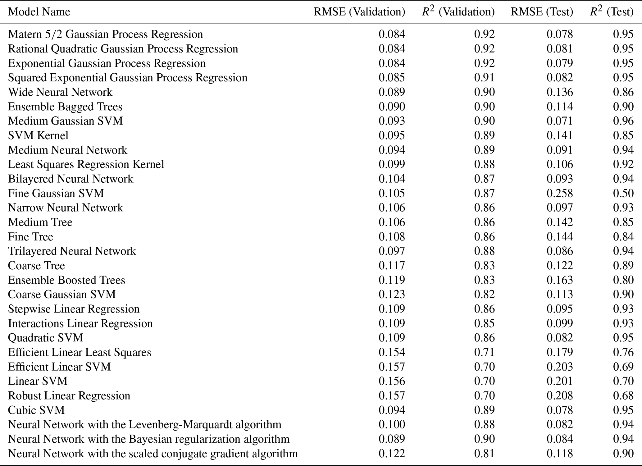
To clarify the division of labor between the two cross-validation strategies, the 10-fold cross-validation was retained exclusively for hyperparameter tuning, while the cruise-separated 5-fold cross-validation focused on evaluating robust performance across synoptic cruise units. Predictive performance for all models was assessed using the Root Mean Squared Error (RMSE) and the coefficient of determination (R²), computed separately for the validation and test sets. Among all tested models, including GPR with the squared exponential and other kernels (Table 2), the Matern $\mathrm{5}/\mathrm{2}$ GPR achieved the best predictive performance (lowest RMSE and highest R²) on both the validation set and the independent test set, while also providing meaningful uncertainty estimates, confirming its superiority for subsequent analysis.

Table 2 Selection of machine-learning models based on Root Mean Squared Error (RMSE), and the coefficient of determination (R²).

The process of developing and reconstructing the δ¹³C_DIC data product is outlined in Fig. 2. Data collection and preprocessing were conducted following the procedures detailed in Sect. 2.1 and 2.2.

The selected quality-controlled 37 cruises were used for model development, validation and test. Two of them (33RO20050111 and 33MW19930704), from the South and North Atlantic respectively, were randomly selected to form an independent test set (X1). The other 35 cruises formed dataset X2, which was further randomly split into a training set (80 %) and a validation set (20 %). The validation set was used to fine-tune hyperparameters and assess model performance, ensuring generalizability and helping identify overfitting (Wu et al., 2025). The model was trained using paired input variables: longitude (lon), latitude (lat), depth, temperature (T), salinity (S), apparent oxygen utilization (AOU), nitrate (N), silicate (Si), DIC, and atmospheric CO₂ (xCO₂), along with corresponding δ¹³C_DIC values as the target variable (Eq. 1).

$$\begin{array}{}\text{(1)}& \begin{array}{rl}{{\mathit{\delta }}^{\mathrm{13}}\mathrm{C}}_{\mathrm{DIC}}& =f(\mathrm{lon},\mathrm{lat},\mathrm{depth},T,S,\mathrm{AOU},\mathrm{N},\\ & \mathrm{Si},\mathrm{DIC},x{\mathrm{CO}}_{\mathrm{2}})\end{array}\end{array}$$

These input variables were selected to comprehensively capture the key physical, biological, and geochemical drivers influencing δ¹³C_DIC. Specifically, longitude, latitude, and depth represent the spatial location of each observation, which is essential for resolving regional and vertical patterns. T and S reflect thermohaline forcing, i.e., the physical processes such as mixing, stratification, and water mass formation that impact carbon cycling. AOU, nitrate, and silicate are indicators of biological forcing, as they are influenced by biological productivity, remineralization, and nutrient utilization. DIC is directly related to δ¹³C_DIC, since δ¹³C_DIC reflects the stable carbon isotopic composition of the DIC pool; thus, variations in DIC are closely tied to changes in δ¹³C_DIC. However, AOU, nutrients, and DIC also reflect partially physics as they are being mixed by ocean circulation. Finally, xCO₂ represents external perturbations from air-sea CO₂ exchange, which can alter both the concentration and isotopic composition of DIC. This term is necessary for predicting recent anthropogenic CO₂ influences on ocean CO₂ parameters, in particular, their decadal change rates.

The independent test set (X1), excluded entirely from training and validation, provides a final evaluation of model performance. Its role in assessing predictive skill across spatial data gaps ensures robust generalization. Finally, the trained GPR model is applied to the full set of hydrographic parameters from the GLODAPv2.2023 Atlantic dataset (https://glodap.info/index.php/merged-and-adjusted-data-product-v2-2023/, last access: 22 March 2026) to reconstruct a basin-wide δ¹³C_DIC distribution over time across the Atlantic Ocean.

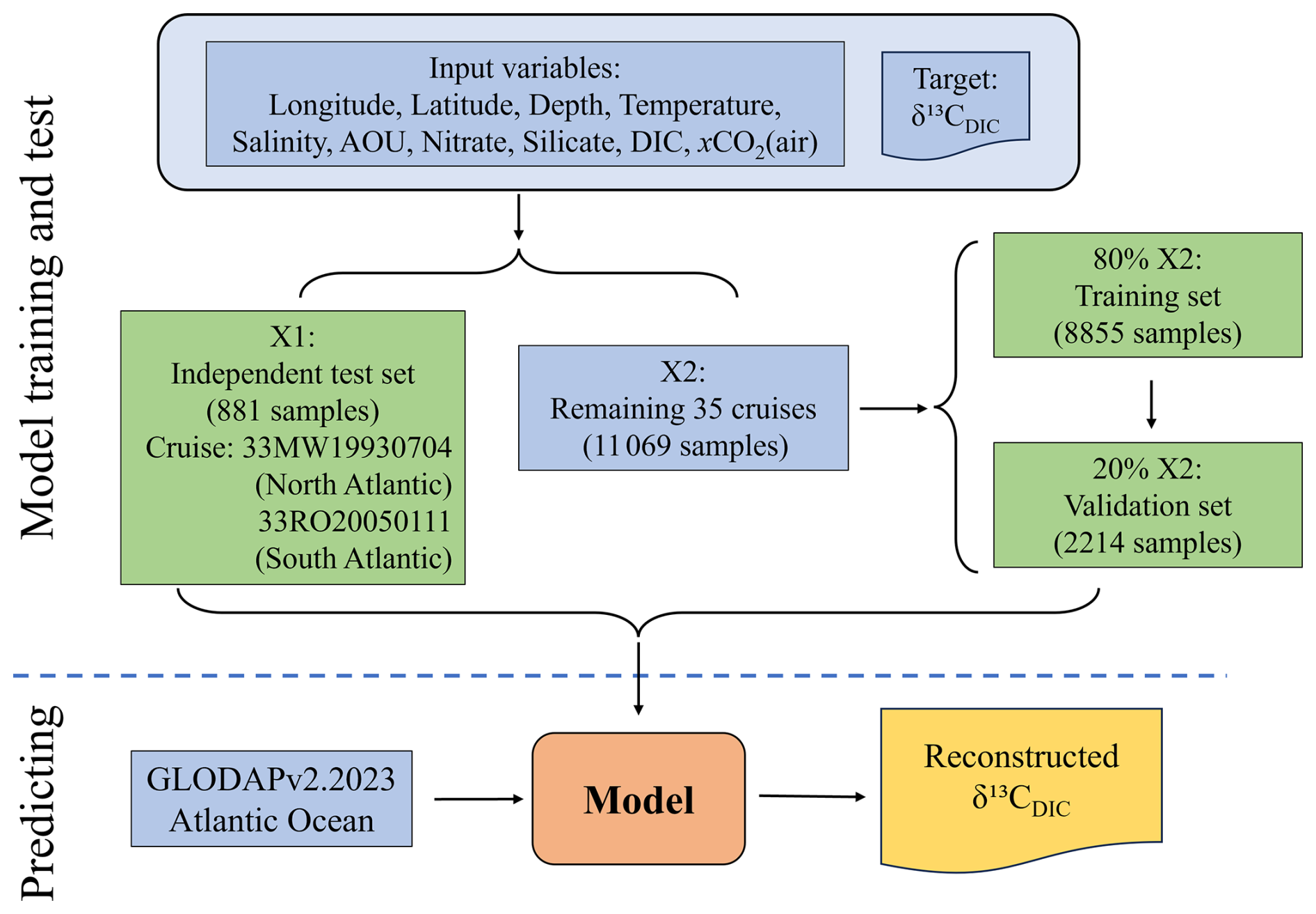
Figure 2 A flowchart illustrating the machine-learning regression model for reconstructing the δ¹³C_DIC product. The blue boxes represent the input, and the yellow box represents output datasets, while the green boxes depict the model training, validation, and independent testing processes. The orange box indicates the final trained model used for prediction.

2.4 Evaluation of model

The accuracy of the model outputs was evaluated using various statistical metrics, including the R², RMSE, mean absolute error (MAE), and mean bias error (MBE). Among these metrics, MAE and MBE are valuable for evaluating the performance of the machine learning models. MAE quantifies the average absolute deviation between observed and predicted values; its insensitivity to outliers makes it ideal for handling the potential noise in δ¹³C_DIC observational data, ensuring a robust measure of overall prediction error. MBE, by retaining the sign of deviations, identifies systematic biases (e.g., consistent overestimation or underestimation of δ¹³C_DIC), which is critical for refining the machine learning model.

These metrics were calculated for the training, validation, and independent test phases, as defined below:

$$\begin{array}{}\text{(2)}& {\displaystyle }{R}^{\mathrm{2}}=\mathrm{1}-{\displaystyle \frac{{\sum }_{i=\mathrm{1}}^N(y_{\mathrm{obs},i}-y_{\mathrm{est},i}{)}^{\mathrm{2}}}{{\sum }_{i=\mathrm{1}}^N(y_{\mathrm{obs},i}-\stackrel{\mathrm{‾}}{y_{\mathrm{obs}}}{)}^{\mathrm{2}}}}\text{(3)}& {\displaystyle }\mathrm{RMSE}=\sqrt{{\displaystyle \frac{\mathrm{1}}{N}}{\sum }_{i=\mathrm{1}}^N(y_{\mathrm{obs},i}-y_{\mathrm{est},i}{)}^{\mathrm{2}}}\text{(4)}& {\displaystyle }\mathrm{MAE}={\displaystyle \frac{\mathrm{1}}{N}}{\sum }_{i=\mathrm{1}}^N\left|y_{\mathrm{obs},i}-y_{\mathrm{est},i}\right|\text{(5)}& {\displaystyle }\mathrm{MBE}={\displaystyle \frac{\mathrm{1}}{N}}{\sum }_{i=\mathrm{1}}^N\left(y_{\mathrm{obs},i}-y_{\mathrm{est},i}\right)\end{array}$$

Here, i represents the ith sample, y_obs,i refers to the observed δ¹³C_DIC, $\stackrel{\mathrm{‾}}{y_{\mathrm{obs}}}$ is the mean of the observed δ¹³C_DIC values, y_est,i denotes the predicted δ¹³C_DIC values from the final model, and N is the total number of matched samples.

2.5 Uncertainty of the reconstructed δ¹³C_DIC

A comprehensive assessment of uncertainty of the reconstructed δ¹³C_DIC was derived via error propagation, assuming independence between distinct uncertainty sources. These sources of uncertainties include: the direct δ¹³C_DIC measurement uncertainty from observations (u_obs), the uncertainty accumulated from the input variables (u_inputs), and the uncertainty induced by the mapping function (u_map). Following standard error propagation protocols (Hughes and Hase, 2010; Taylor, 1997), the comprehensive uncertainty of our estimated δ¹³C_DIC product, $u_{{\mathit{\delta }}^{\mathrm{13}}{C}_{\mathrm{DIC}}}$, was calculated as the root sum of the squares of the individual uncertainties:

$$\begin{array}{}\text{(6)}& u_{{\mathit{\delta }}^{\mathrm{13}}{C}_{\mathrm{DIC}}=\sqrt{u_{\mathrm{obs}}^{\mathrm{2}}+u_{\mathrm{inputs}}^{\mathrm{2}}+u_{\mathrm{map}}^{\mathrm{2}}}}\end{array}$$

The observational uncertainty u_obs inherent in δ¹³C_DIC measurements varies by analytical method. For samples, when it is analyzed using IRMS, reported uncertainties range from ±0.12 ‰ (Gruber et al., 1999) to ±0.03 ‰ (Quay et al., 2003). For CRDS analysis, uncertainties are reported as ±0.07 ‰ for cruise 33RO20200321 (Gao et al., 2024) and ±0.03 ‰ for cruises 33RO20230306 and 33RO20230413 (Sun et al., 2025). Taking a conservative approach, we adopted an average u_obs value of 0.07 ‰.

The input variable uncertainty (u_inputs) accounts for uncertainties in temperature, salinity, nitrate, silicate, DIC, alkalinity, and xCO₂. Monte Carlo simulation is performed 1000 times to quantify u_inputs. Following Carter et al. (2024) and Wu et al. (2025), the perturbation of 0.002, 0.002, 2, 0.4, 0.4, 2 and 0.2 are randomly applied to temperature, salinity, AOU, nitrate, silicate, DIC, and xCO₂, respectively. We then recalculated δ¹³C_DIC using these perturbed inputs and quantified the resulting changes. The uncertainty contribution from each variable was determined as the standard deviation of the differences between the original reconstructed δ¹³C_DIC and the noise-perturbed values. The final u_inputs was calculated as the square root of the quadratic sum of these individual uncertainties.

$$\begin{array}{}\text{(7)}& u_{\mathrm{inputs}}^{\mathrm{2}}=u_T^{\mathrm{2}}+u_{\mathrm{S}}^{\mathrm{2}}+u_{\mathrm{AOU}}^{\mathrm{2}}+u_{\mathrm{N}}^{\mathrm{2}}+u_{\mathrm{Si}}^{\mathrm{2}}+u_{\mathrm{DIC}}^{\mathrm{2}}+u_{x{\mathrm{CO}}_{\mathrm{2}}}^{\mathrm{2}}\end{array}$$

The uncertainty associated with the mapping function, u_map, is introduced within the GPR model. Here, u_map is primarily quantified using the GPR model's posterior predictive standard deviation (i.e., the square root of the posterior predictive variance), that is, GPR uncertainty. GPR uncertainty is a conceptually direct measure that reflects the model's inherent uncertainty in mapping environmental predictors to δ¹³C_DIC across the entire prediction set. The mean value of this GPR-derived u_map is 0.08 ‰ across the prediction set, which captures both model variability and uncertainty related to generalization to unobserved regions. Wu et al. (2025) suggested that u_map may alternatively be estimated as the RMSE between reconstructed and observed δ¹³C_DIC on the reconstruction dataset, and we additionally report this RMSE as a reference to facilitate compatibility. Notably, the two metrics are quantitatively similar, ensuring our core uncertainty estimate remains consistent with widely adopted reporting practices while prioritizing the GPR-derived measure's scientific rigor.

3 Results and Discussion

3.1 Evaluation of the GPR model performance

The trained GPR model exhibited robust performance and high accuracy in representing δ¹³C_DIC characteristics across the Atlantic Ocean (Fig. 3). During the training phase, we leveraged a 10-fold cross-validation approach, selected as it is a standard pre-implemented option in MATLAB's Machine Learning Toolbox. This approach balances computational efficiency and robustness, reducing overfitting by iteratively splitting training data into 10 folds: 9 for training and 1 for validation per iteration, with results averaged across iterations to ensure stable performance. Finally, the model with 10-fold cross-validation achieved an R² of 0.92, an RMSE of 0.083 ‰, an MAE of 0.056 ‰, and an MBE of −0.0003 ‰ during training phase (Fig. 3a). Performance metrics during the validation phase (Fig. 3b) were comparable to those in the training phase, demonstrating the model's strong generalization ability, i.e., its capacity to accurately predict data not used for training, and confirming its resistance to overfitting. Additionally, in the independent testing phase, the model also maintained high accuracy (R² = 0.95, RMSE = 0.082 ‰, MAE = 0.056 ‰, MBE = 0.007 ‰, Fig. 3c), with most samples clustered closely around the 1:1 line. These results indicate that the model can reliably predict δ¹³C_DIC across diverse, unobserved spatial and temporal scales.

To further verify the model's robustness across different cruise combinations, we additionally conducted a cruise-separated 5-fold cross-validation. This supplementary cross-validation also yielded stable performance across all folds: per-fold RMSE ranged from 0.097 ‰ to 0.156 ‰ with an average of 0.124 ‰ (±0.027 ‰, standard deviation), and per-fold adjusted R² ranged from 0.74 to 0.92 with an average of 0.80 (±0.08, standard deviation). The small standard deviations of these metrics indicate that the model's performance is not sensitive to the specific combination of training cruises, confirming no significant overfitting caused by uneven sample sizes across cruises and further reinforcing the reliability of the training results. Collectively, these findings, including stable performance in 10-fold cross-validation, reliable results from the cruise-separated 5-fold cross-validation, consistent accuracy in the validation phase, and high reliability in independent testing, demonstrate that the GPR-based δ¹³C_DIC reconstruction method is highly generalizable and robust, enabling it to accurately capture the characteristics in δ¹³C_DIC and provide reliable predictions across the Atlantic Ocean.

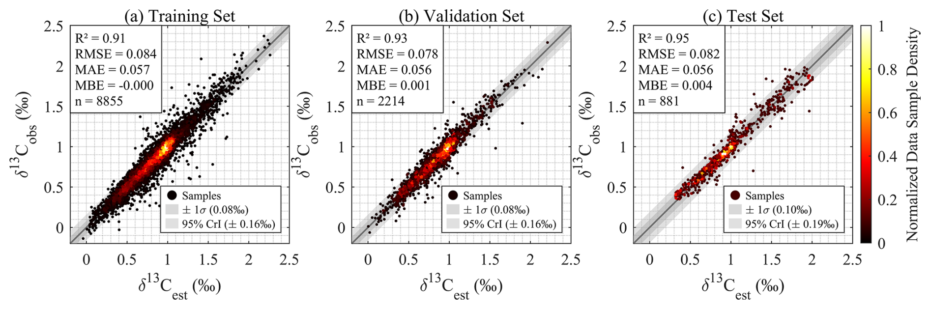
Figure 3 Regression model evaluation for δ¹³C_DIC reconstruction: Density scatter plots comparing model-estimated (δ¹³C_est) versus observed (δ¹³C_obs) δ¹³C_DIC values during (a) training (80 % samples from 35 cruises, with 10-fold cross-validation), (b) validation (20 % samples from 35 cruises), and (c) independent testing (samples from cruises 33RO20050111 and 33MW19930704). Statistical metrics include coefficient of determination (R²), root-mean-square error (RMSE), mean absolute error (MAE), mean bias error (MBE), and sample size (n). Color indicates normalized local data point density within 2D bins: the plot area is divided into a 100 × 100 grid, raw density is the number of points per bin, and values are normalized to 0∼ 1 (0= sparsest, 1 = densest). Shaded bands represent predictive uncertainty, with the darker grey band showing one standard deviation (±1σ) and the lighter grey band showing the 95 % credible interval (CrI).

3.2 Evaluation of the spatial distribution of δ¹³C_DIC

To assess the product's ability to capture δ¹³C_DIC spatial patterns and quantify biases, we utilized the δ¹³C_DIC distribution from independent test cruises 33MW19930704 and 33RO20050111 (Fig. 4). Both cruises are part of the repeated observation A16, specifically A16N (1993) and A16S (2005), which traverses the entire Atlantic Ocean from the sub-Arctic to the Southern Ocean (Fig. 4a). This transect has been frequently used in existing research and textbooks to represent Atlantic-scale distributions of carbonate chemistry and other characteristics (i.e., Wanninkhof et al., 2010; Eide et al., 2017; Millero, 2013), thus it is selected for evaluating the product's regional applicability.

The spatial patterns of model-estimated isotope values (δ¹³C_est) along cruises 33MW19930704 and 33RO20050111 effectively captured the distributional characteristics of the observed values (δ¹³C_obs) (Fig. 4b vs. 4c). The reconstructed δ¹³C_DIC product exhibited a very low transect-mean bias of −0.007 ‰ with a standard deviation of 0.082 ‰ (Fig. 4d), highlighting the product's reliability in estimating the spatial distribution of δ¹³C_DIC. Spatially, the discrepancies are very small in most regions of the transect, but relatively larger in subpolar regions (around 50° S or 50° N) and vertically in the upper 500 m and below 3000 m (Fig. 4d).

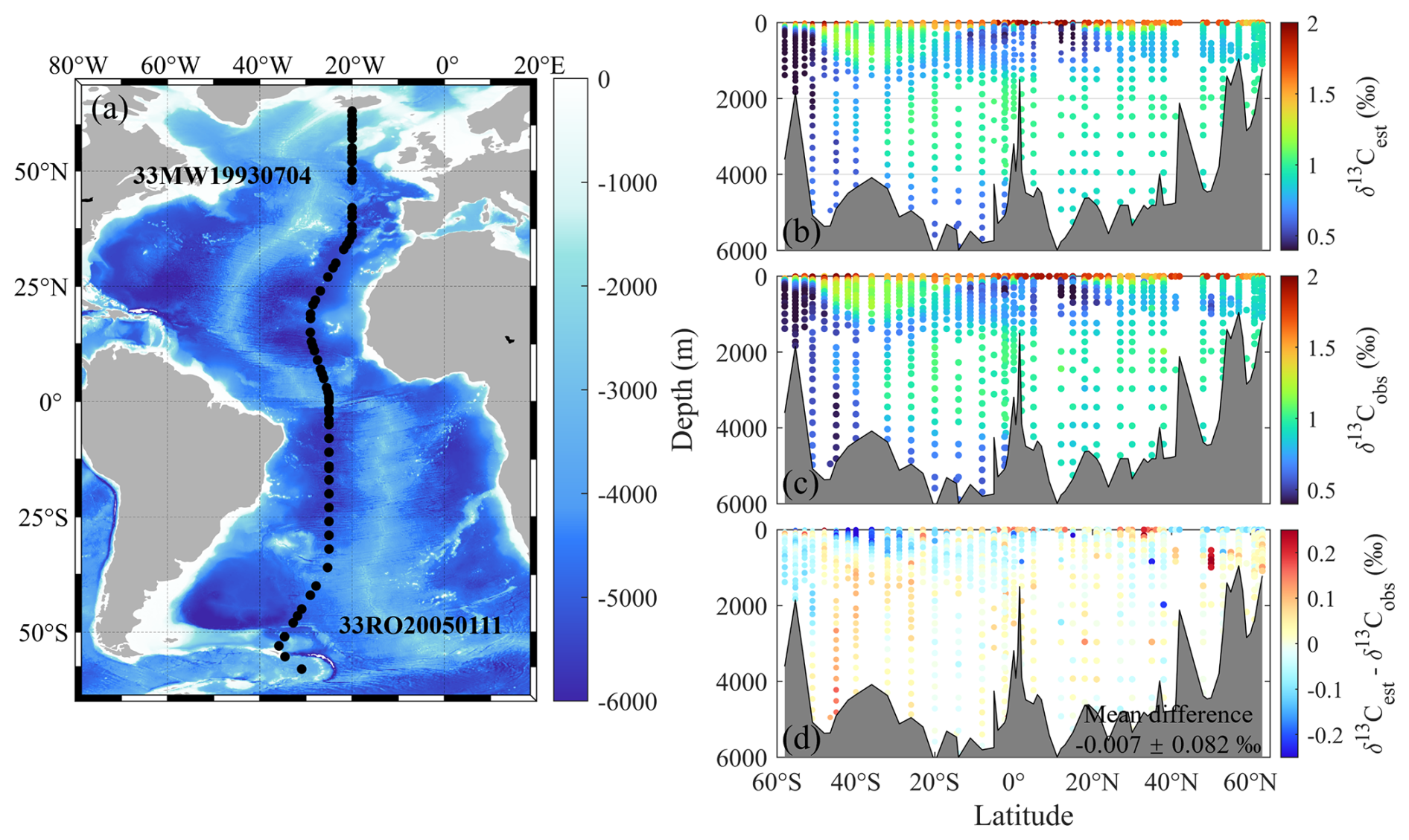
Figure 4 (a) Station locations of the independent test cruises 33MW19930704 and 33RO20050111; Depth profile of (b) model-estimated (δ¹³C_est) and (c) in-situ observed (δ¹³C_obs) δ¹³C_DIC along cruises 33MW19930704 and 33RO20050111, and (d) spatial distribution of mean bias error (MBE) between δ¹³C_est and δ¹³C_obs for the two cruises. Positive MBE values (red) denote product overestimation, while negative values (blue) indicate underestimation relative to observation. The overall mean difference is −0.007 ± 0.082 ‰.

3.3 Evaluation of the product's uncertainty

The uncertainty of the reconstructed δ¹³C_DIC product was estimated by propagating uncertainties from three primary sources: measurement (u_obs), input variables (u_inputs) and mapping (u_map). Detailed calculations are described in Sect. 2.5 of the Methods. To ensure a conservative estimate, we adopted a uniform u_obs of 0.07 ‰ for all data points. u_map is primarily quantified using the GPR model's posterior predictive standard deviation (i.e., the square root of the posterior predictive variance), which reflects the model's inherent uncertainty in mapping environmental predictors to δ¹³C_DIC and captures both model variability and generalization-related uncertainty to unobserved regions. The mean value of this GPR-derived u_map is 0.08 ‰. Following previous literature (Wu et al., 2025; Roobaert et al., 2024; Sharp et al., 2022), u_map can alternatively be estimated as the RMSE between δ¹³C_est and δ¹³C_obs in the training set. We additionally report this RMSE-based metric as a reference for compatibility with existing studies, and notably, it yields a quantitatively similar value of 0.08 ‰ to the GPR-derived u_map. u_inputs was quantified via Monte Carlo simulation, considering contributions from seven environmental variables: T, S, AOU, N, Si, DIC, xCO₂. Notably, uncertainties from input variables had a nearly negligible impact, with u_inputs estimated at 0.009 ‰ . The u_inputs contribution from individual input variables was decomposed as follows: temperature (4.96 × 10⁻⁵ ‰), salinity (3.62 × 10⁻⁴ ‰), nitrate (0.004 ‰), silicate (0.002 ‰), DIC (0.005 ‰), AOU (0.004 ‰), and xCO₂ (6.52 × 10⁻⁴ ‰). Overall, the reconstructed δ¹³C_DIC product exhibits an average uncertainty of 0.11 ‰ for the entire Atlantic Ocean. This uncertainty is considered reasonable given the conservative estimation approach, highlighting the product's reliability for δ¹³C_DIC characterization.

3.4 Additional validation using data extracted from a numerical model environment

To address the inherent limitation of observational δ¹³C_DIC data (sparse and unevenly distributed across space and time), we conducted supplementary numerical model-based validation to verify the GPR model's reliability. This validation utilized well-validated ocean carbon isotope simulation data from Claret et al. (2021), which includes global monthly outputs (1990–2002) with a 1° × 1° horizontal grid and 50 depth layers (Appendix A).

First, we focused on the Northeast Atlantic (30° W–5° W, 5° S–66° N) and downsampled the data to simulate observational sparsity. Limited by computational resources, we selected data from 1991 to 1995 (60 months) for validation, with 1993 (12 months) designated as an independent test set to assess generalization (Appendix A1.2). The GPR model adopted the same configuration as the observational-based reconstruction (Matern $\mathrm{5}/\mathrm{2}$ kernel, 10-fold cross-validation for hyperparameter tuning). Validation results demonstrated exceptional performance. For raw δ¹³C_DIC values, R² exceeded 0.99 and RMSE was less than 0.015 ‰ across the training set, independent test set, and additional prediction set (Figs. A1 and A2 in Appendix A1.3). Additionally, anomaly-based R² (quantifying deviations from local climatological means) ranged from 0.67 to 0.90, confirming the model's ability to capture biogeochemically meaningful spatiotemporal variations independent of large-scale offsets. For detailed data processing, parameter settings, and full validation results, refer to Appendix A1.

Second, to further enhance the credibility of the GPR model in real-world application scenarios, we supplemented an additional observation-constrained sparse validation based on the same numerical model dataset (Appendix A2). This validation strictly mimics the spatial locations of sparse oceanographic observations by subsampling model data exclusively at the exact locations of the 37 Atlantic cruises and GLODAP locations, while preserving cruise-specific uneven sampling patterns (full experimental design detailed in Appendix A2.1). The results of this supplementary validation also showed robust performance. The training set achieved an R² of 0.99 and an RMSE of 0.009 ‰, the independent test set yielded an R² of 0.99 and an RMSE of 0.025 ‰, and the reconstructed values at GLODAP locations were highly consistent with the model's native values (R²=0.95, RMSE = 0.080 ‰) (Figs. A3 and A4, see Appendix A2.3 for details).

We further conducted a supplementary full Atlantic domain generalization test to verify the model's ability to reproduce large-scale δ¹³C_DIC patterns across the entire basin. Using the model trained on observation-matched sparse data, we predicted gridded δ¹³C_DIC values for the full Atlantic domain, with results showing strong overall alignment with the native model values (R²=0.83, RMSE = 0.193 ‰ across 8.4 million valid samples, Fig. A5 in Appendix A3). This test provides additional evidence that our approach can reliably leverage sparse observations to estimate basin-scale oceanographic δ¹³C_DIC distributions.

The grid-based downsampling validation and the supplementary observation – constrained sparse validation complement each other, jointly verifying the GPR model's robustness in reconstructing δ¹³C_DIC patterns from sparse data, whether under idealized sparse grid scenarios or real observational sparse scenarios. This dual validation framework provides a solid methodological foundation for subsequent observational-based reconstruction.

3.5 Reconstruction of δ¹³C_DIC

Here, the trained GPR model is applied to GLODAPv2.2023 hydrographic data for δ¹³C_DIC reconstruction in the Atlantic Ocean, spanning the 1980s to 2021 with a small number of 1972 data points. The GLODAPv2.2023 Atlantic dataset comprises 500 137 samples, of which 8941 contain acceptable δ¹³C_DIC observations (quality flags = 2 or 6). A total of 124 643 δ¹³C_DIC values can be reconstructed based on the availability of all required predictor variables (salinity, AOU, Nitrate, Silicate, and DIC). Among these, 68 435 reconstructions are considered high quality, as all six input variables have acceptable quality flags, which is approximately 7.65 times larger than the number of δ¹³C_DIC observations. The remaining 56 208 reconstructions are based on input variables with unknown or lower quality and are thus assigned a quality flag of 3 (questionable). All 124 643 reconstructions, 13.9 times larger than the observation, are provided in the supplementary Dataset, of which the questionable δ¹³C_DIC samples are provided for transparency but are not recommended for routine use without further quality assessment. The following presentations and analyses are restricted to the 68 435 acceptable samples to ensure the robustness of the results unless otherwise noted.

The observed and reconstructed datasets share an intersection of 5997 samples that have both acceptable δ¹³C_DIC observations and acceptable input variables for reconstruction. These overlapping samples are used for direct model evaluation (Fig. 5a). The comparison between observed and reconstructed δ¹³C_DIC values yields a high correlation coefficient (R²=0.89), with RMSE = 0.094 ‰, MAE = 0.067 ‰, and MBE $=-$0.009 ‰. The mean difference between reconstruction and observation is −0.009 ± 0.097 ‰, confirming strong overall agreement. To further verify the statistical consistency between observed and reconstructed δ¹³C_DIC values, we calculated Gaussian kernel density estimation (KDE) for both datasets (Fig. 5b). KDE is a non-parametric method for approximating probability density functions by summing Gaussian kernel functions centered at each data point (Silverman, 1986), producing a continuous estimate that is less sensitive to arbitrary bin edges. For this analysis, KDE was applied on a uniform grid spanning the full δ¹³C_DIC range, with a bandwidth of 0.1 ‰ chosen to balance smoothing and resolution. No additional jittering was applied as the data contains sufficient variability to avoid overlapping artifacts. The KDE curves of observed (n = 8941, range from −0.37 ‰ to 2.37 ‰) and reconstructed (n = 68 435, range from −0.11 ‰ to 2.36 ‰) δ¹³C_DIC are highly consistent, exhibiting nearly identical unimodal distributions, with a primary peak around 1 ‰. Both curves decline rapidly to near zero at the extremes (below ∼ 0 ‰ and above ∼ 2 ‰), reflecting minimal occurrence of δ¹³C_DIC values in these ranges. This close alignment confirms the reconstructed δ¹³C_DIC from GPR model accurately captures the central tendency, overall shape, and range of the observed δ¹³C_DIC distribution.

The reconstructed dataset, which has a much larger sample size and spatially continuous coverage, exhibits minimally higher probability density than observations for δ¹³C_DIC values between approximately 0.8 ‰ and 1.1 ‰, alongside a slightly sharper peak and reduced variance. This subtle distinction is a natural consequence of model smoothing intrinsic to GPR's Gaussian kernel framework and the mitigation of sampling noise in the dense, continuous reconstruction. By weighting neighbouring data points to produce spatially consistent predictions, GPR avoids overfitting to sparse extreme values often linked to transient perturbations or observational noise, an outcome aligned with the study's objective of generating a robust, representative δ¹³C_DIC distribution. Overall, the KDE analysis, based on a systematic bandwidth selection and grid evaluation, underscores the strong statistical congruence between observed and reconstructed δ¹³C_DIC, with the minor differences being negligible relative to the model's success in replicating the core characteristics of the observed distribution.

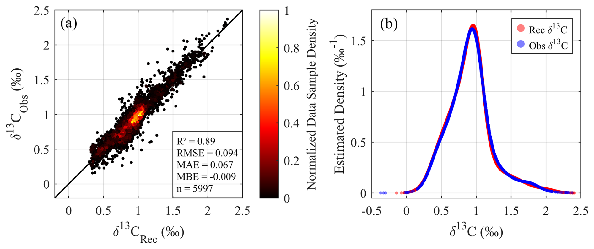
Figure 5 Comparison of observed and reconstructed δ¹³C_DIC values derived from the GLODAPv2.2023 dataset. (a) Density scatter plot of observed versus reconstructed δ¹³C_DIC values, using only the intersection of data points with acceptable quality available in both observed and reconstructed datasets (n=5997). (b) Gaussian kernel density estimations (KDEs) for a comprehensive evaluation of observed and reconstructed δ¹³C_DIC values. In panel (b), the blue curve represents all acceptable δ¹³C_DIC observations (n=8941), while the red curve indicates all acceptable reconstructed δ¹³C_DIC values (n=68 435), generated by GPR model trained on the GLODAPv2.2023 dataset. The KDEs reveal the overall distribution shape, highlight differences in peak height and spread, and provide a smooth, continuous representation of probability density.

The GLODAPv2.2023 Atlantic Ocean dataset includes approximately 20 583 stations in total (Fig. 6a). Among these, only about 732 stations have δ¹³C_DIC observations (blue points in Fig. 6b), collected over the four decades, reflecting the limited spatial and temporal extent of direct observations due to the high cost and complexity of δ¹³C sampling and analysis. Using the proposed GPR model, δ¹³C_DIC values have been reconstructed at roughly 4182 stations (red points in Fig. 6b). This reconstructed dataset significantly expands both temporal and spatial coverage of δ¹³C_DIC in the Atlantic Ocean, enabling more detailed and extensive biogeochemical analyses across the Atlantic.

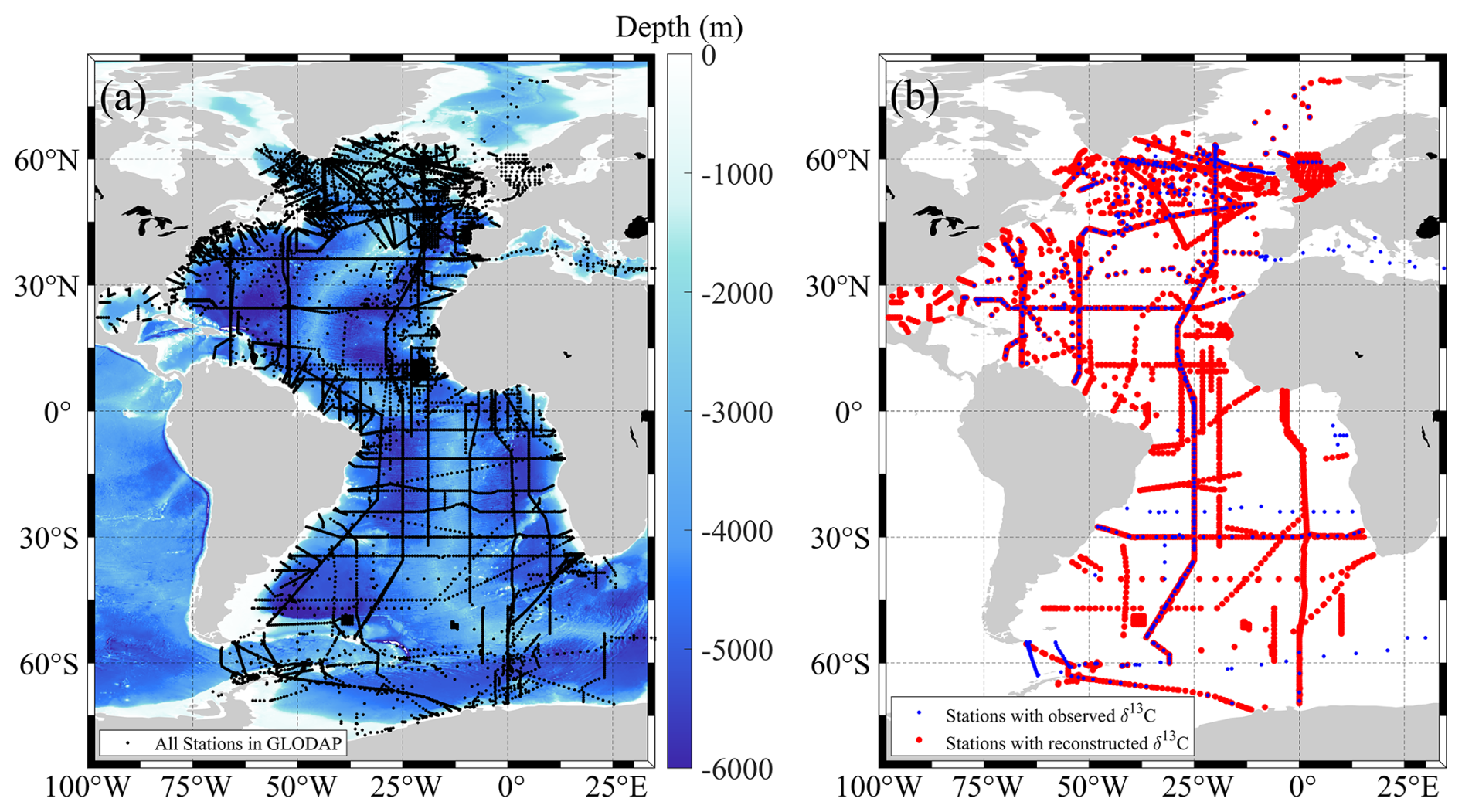
Figure 6 Station maps for the GLODAPv2.2023 Atlantic Ocean dataset. (a) Locations of all stations included in the dataset. (b) Stations with observed (blue dots) and reconstructed (red dots) δ¹³C_DIC.

To evaluate the spatial and temporal coverage expansion of the reconstructed δ¹³C_DIC dataset, the data distributions are compared along longitude, latitude, year, and depth (Fig. 7). Along longitude (Fig. 7a), the number of reconstructed δ¹³C_DIC increased several times compared to the observed, and also extended into west of 70° W and east of 0° E where there are almost no direct δ¹³C_DIC observations. The latitudinal distribution (Fig. 7b) shows notable improvements in both hemispheres. The reconstructed dataset greatly enhanced the temporal coverage (Fig. 7c). There is little to no reconstructed data before 1980, between 1984 and 1987, and in 1995. The number of reconstructed data increases significantly after the late-1980s, reaching a peak in 2003, (Fig. 7c). Vertically, the data number of reconstructed δ¹³C_DIC increased substantially throughout the water column, although numbers of both reconstructed and observed δ¹³C_DIC data show exponential decrease from surface to deep water (Fig. 7d).

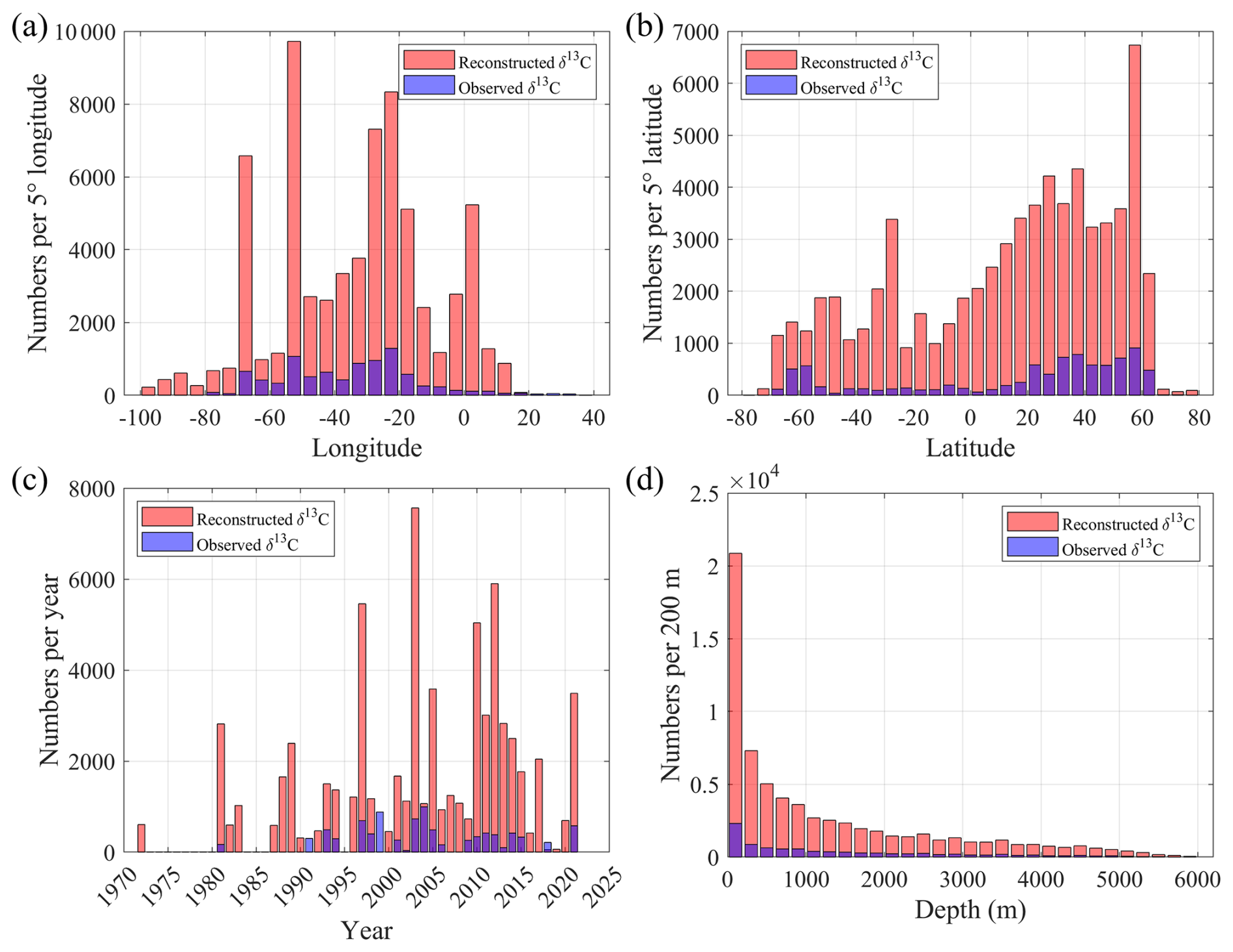
Figure 7 Comparison of the spatial, temporal, and vertical distributions of observed and reconstructed δ¹³C_DIC data in the Atlantic Ocean. The number of δ¹³C_DIC samples is shown by (a) longitude (per 5° bin), (b) latitude (per 5° bin), (c) year (from 1972 to 2021), and (d) depth (per 200 m interval). Red bars represent reconstructed δ¹³C_DIC, and blue bars indicate observed δ¹³C_DIC.

Overall, the reconstructed δ¹³C_DIC dataset consistently demonstrated good accuracy, high correlation coefficient, low RMSE, MAE, and minimal bias across diverse environmental conditions. Spatially, the reconstruction significantly expands coverage across longitude, latitude, and depth, particularly in undersampled regions such as the South Atlantic and deeper ocean. Temporally, it enhances data availability, filling many before 1990 and after 2015, despite some limitations tied to input variable availability.

Additionally, a spatially continuous 3D (1° × 1° horizontal resolution, 33 standard depth layers) climatological δ¹³C_DIC dataset for the Atlantic Ocean was generated using the validated GPR framework. This product was built on gridded environmental predictors (temperature, salinity, oxygen (used to calculate AOU), nitrate, silicate, and DIC) from the GLODAPv2 1° × 1° global interior ocean mapped climatology (Lauvset et al., 2016) and monthly mean atmospheric xCO₂ spanning 1972–2013. The resulting product aligned with the coordinate system and structural conventions of the GLODAPv2 gridded framework, ensuring full interoperability with mainstream ocean biogeochemistry research workflows. It is specifically designed to address the critical limitations of discrete site-level δ¹³C_DIC observations for basin-scale spatial analyses. This gridded product is archived alongside our other datasets in the Zenodo repository (https://doi.org/10.5281/zenodo.18481145, Gao et al., 2025).

3.6 Potential Applications

The improved spatial, temporal, and vertical coverage of the reconstructed δ¹³C_DIC dataset potentially contributes to the biogeochemical research and to a deeper understanding of carbon cycling processes in the Atlantic Ocean. Two specific applications are given as examples here: (1) examining the spatial patterns and decadal variability of surface δ¹³C_DIC (≤ 10 m), and (2) evaluating its ability to resolve vertical profiles, thereby providing insights into subsurface carbon dynamics.

To facilitate a more comprehensive understanding of the spatial and temporal dynamics of surface δ¹³C_DIC in the Atlantic, Fig. 8 illustrates how the reconstruction improves the spatial representativeness and temporal continuity of surface δ¹³C_DIC. The expanded spatial coverage shown in Fig. 8a increases the representativeness of latitudinal sample bins, reducing the influence of sparsely sampled outliers on bin means (Fig. 8b). For instance, observational data in the 5–10° S band during the 2000s show an anomalously low mean that is likely driven by a few isolated observations. In contrast, the reconstructed dataset, by supplying a larger and spatially coherent sample set, yields a mean that is more consistent with adjacent latitude bands. This effect should be understood as a reduction of sampling-driven discontinuities and noise rather than as an artificial suppression of genuine signals. Both observed and reconstructed data indicate a basin-scale decline in surface δ¹³C_DIC from the 1980s to the 2010s, most pronounced in tropical and subtropical regions (approximately 35° S–35° N), consistent with the expected Suess effect from increasing fossil-fuel CO₂ (Keeling, 1979). In contrast, the mid- to high-latitude regions exhibit more complex variability, likely reflecting the influence of regional circulation, water mass formation, and subduction processes that modulate isotopic signals on multi-decadal timescales.

To facilitate a clear and intuitive assessment of decadal distributions of observed and reconstructed surface δ¹³C_DIC, we employ KDE. KDE results presented in Fig. 8c are computed using all acceptable observed and reconstructed surface δ¹³C_DIC samples within each decade and are intended to reveal the overall distributional characteristics and their evolution across decades and complement the latitude-binned means shown in Fig. 8b. In general, both observed and reconstructed KDE curves confirm the decadal downward shifts of δ¹³C_DIC from the 1980s to the 2010s, reinforcing the notion of a basin-wide isotopic response to anthropogenic carbon inputs. And the observed and reconstructed KDE curves within each decade fall within comparable value ranges and exhibit similar peak positions, underscoring the consistency between the two datasets. Notable discrepancies arise in specific decades. For instance, in the 1980s the reconstructed KDE curve shows a dominant peak near 2 ‰ and a secondary peak near 1.7 ‰. The latter closely corresponds to the single, broader maximum in the observational KDE curve. This discrepancy is likely attributable to the sparse observational coverage during this decade (Fig. 8a), which limits the representativeness of the latitudinal distribution. In the 2000s, the reconstructed KDE curve exhibits slightly greater density at the lower end of the common range (∼ 0.5 ‰–2.0 ‰) than the observational KDE curve, producing a modest negative shift in central tendency while maintaining a comparable overall span. This shift is primarily attributable to a disproportionate increase in reconstructed data between 50 and 65° N, which modifies the density structure of the distribution. These examples highlight that the reconstruction not only reproduces the principal features of the observational distributions but also mitigates the limitations imposed by sparse or uneven sampling. The reconstructed KDE curves are generally smoother and more spatially coherent than the raw observational KDE curves. The smoother and more coherent appearance of the reconstructed KDE curves reflect the underlying basin-scale δ¹³C_DIC structure. This enhanced spatial consistency allows the basin-wide decadal shift toward lower δ¹³C_DIC values to emerge more clearly by reducing the influence of uneven sampling. As a result, the reconstruction provides a more representative depiction of δ¹³C_DIC variability across latitude and time, improving the statistical robustness and interpretability of the inferred distributional changes.

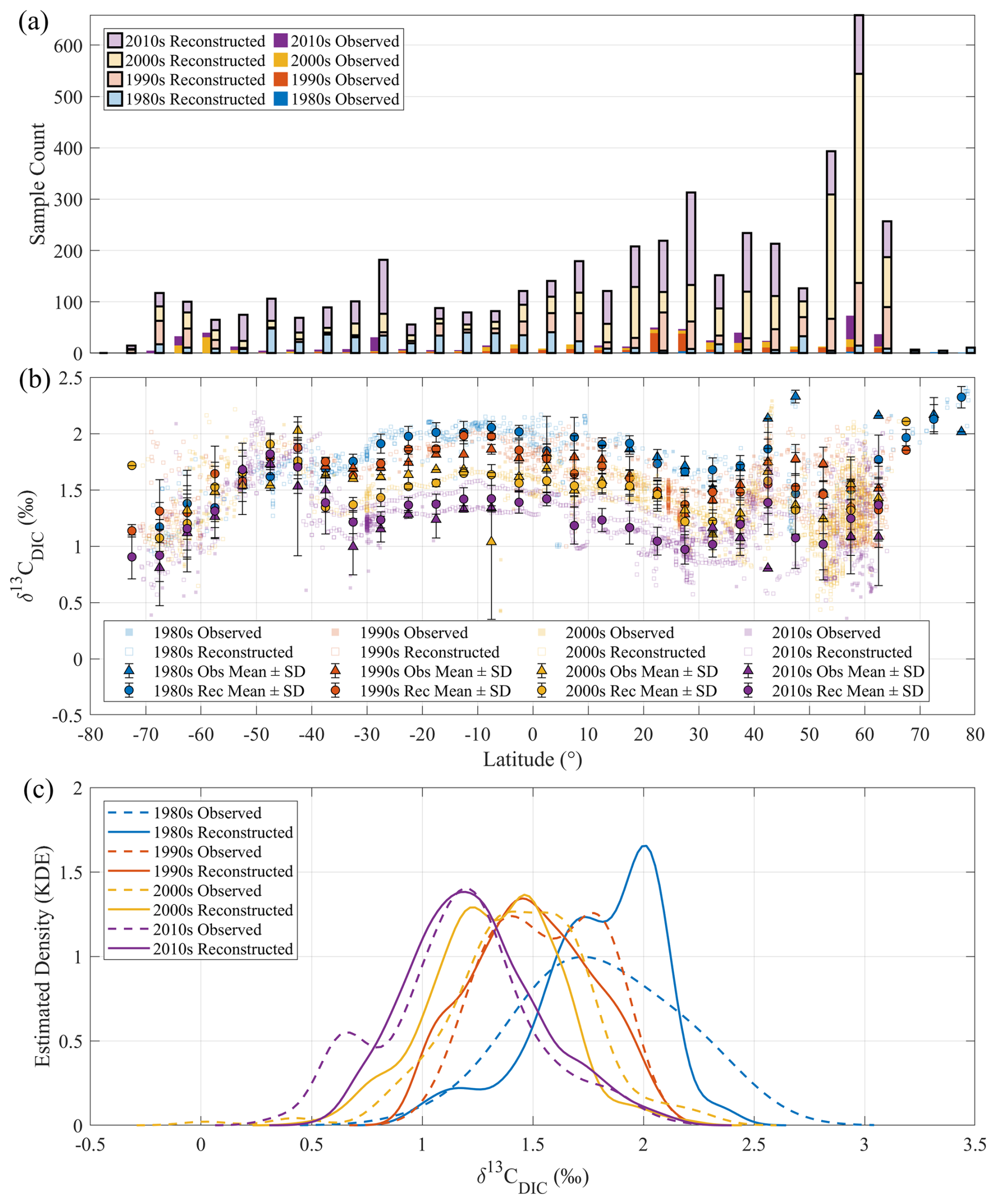
Figure 8 Surface distribution of observed and reconstructed δ¹³C_DIC in the Atlantic Ocean across four decades. (a) Number of observed and reconstructed δ¹³C_DIC samples within each 5° latitude band for the 1980s, 1990s, 2000s, and 2010s. For each latitude band, stacked bars represent decadal sample counts. Solid (opaque) bars indicate observations, and semi-transparent bars with black outlines indicate corresponding reconstructions. (b) Surface δ¹³C_DIC distributions (depth ≤ 10 m) along latitude for the 1980s, 1990s, 2000s, and 2010s. Colored scatter points indicate individual δ¹³C_DIC values from observations (circles) and reconstructions (dots), while the black markers with corresponding face color and error bars represent the mean ± standard deviation of δ¹³C_DIC within each 5° latitude bin, triangles for observed data and diamonds for reconstructed values. (c) Gaussian kernel density estimates (KDEs) of surface δ¹³C_DIC for each decade (1980s–2010s), using dashed lines for observations and solid lines for reconstructions. These KDEs reveal the decadal evolution and overall distributional characteristics of δ¹³C_DIC in both datasets.

Besides horizontal distributions, the reconstructed δ¹³C_DIC dataset also provides valuable insights into vertical variability. The depth profiles along the North Atlantic A16N transect in 1993, 2003, 2013, and 2023 (Fig. 9) show that the reconstruction substantially improves vertical resolution and continuity, especially for years with sparse measurements. For instance, the δ¹³C_DIC samples were increased from 493 to 1618 in 1993, 38 to 2395 in 2003, and 473 to 2787 in 2013, respectively, enhancing data coverage across depths and latitudes, facilitating the detection of temporal trends associated with ocean carbon uptake and redistribution (Fig. 9). The reconstructed δ¹³C_DIC values for 1993, 2003, and 2013 were generated by applying the pre-trained model to input variables from the GLODAPv2.2023 Atlantic dataset. Notably, as the observational data along A16N in 2023 not included in the GLODAPv2.2023 dataset, we used the same pre-trained and validated model, relying solely on the 2023 observational input variables to produce the reconstructed values. The close alignment between 2023's reconstructed and observed data (Fig. 9d vs. 9h) not only reflects the model's reliability but also validates its ability to generalize, strengthening confidence in reconstructions for years with sparse measurements (e.g., 2003 with only 38 observations).

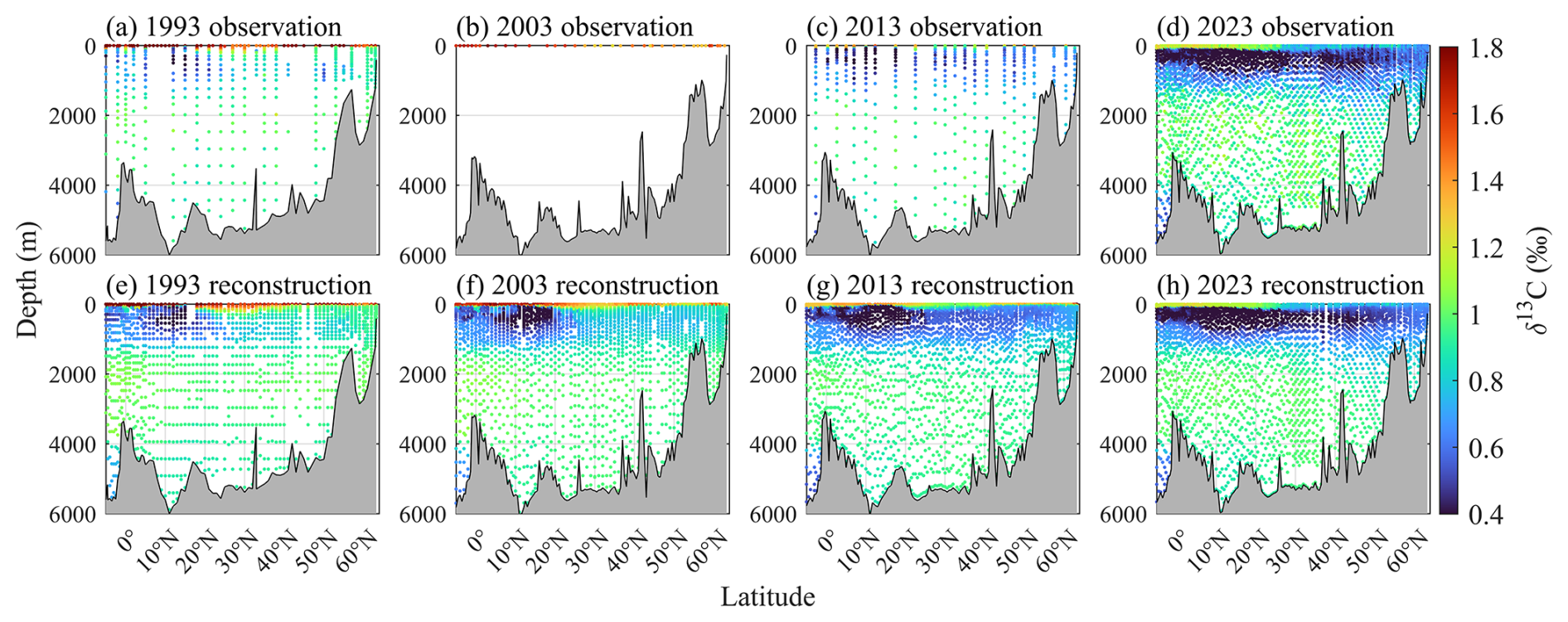
Figure 9 Enhancement of spatial resolution for δ¹³C_DIC through GPR model reconstruction along North Atlantic A16N transect. Top panels (a)–(d) present in-situ observed δ¹³C_DIC from cruises in (a) 1993 (n=493), (b) 2003 (surface-only, n=38), (c) 2013 (n=473), and (d) 2023 (n=3460). Bottom panels (e)–(h) show corresponding reconstructed δ¹³C_DIC with systematic filling of spatial gaps: (e) the number of reconstructed δ¹³C_DIC for cruise A16N in 1993 is 1618; (f) full-depth reconstruction for cruise A16N in 2003 (n=2395); (g) 2013 reconstruction (n=2787), highlighting improved coverage compared to limited observations (n=473); (h) the reconstruction of cruise A16N in 2023 (n=3030) validated against high-density observations. Reconstruction effectively resolves historical sampling sparsity, yielding consistent spatial resolution comparable to contemporary DIC measurements.

The enhanced vertical profiles provided by the reconstructed δ¹³C_DIC dataset also enable more refined investigations into the physical and biological controls governing carbon isotope variability in the ocean interior. Joint interpretation of δ¹³C_DIC with nutrients such as phosphate allows for the identification of water mass structures and biological removal and addition, shedding light on processes such as organic carbon export, remineralization, and the coupling between biological productivity and ocean circulation (e.g., Gruber et al., 1999; Eide et al., 2017). These capabilities improve the isolation of the vertical imprint of the Suess effect and facilitate the reconstruction of preindustrial δ¹³C_DIC, both of which are critical for assessing anthropogenic perturbations to the marine carbon cycle (Olsen and Ninnemann, 2010).

δ¹³C_DIC also can be used to estimate biological carbon export and net community production (NCP) (Quay et al., 2009; Yang et al., 2019). Accurate NCP estimation from δ¹³C_DIC requires knowledge of both the physical supply of DIC and δ¹³C_DIC, typically represented by the subsurface to surface δ¹³C_DIC gradient. Sparse historical δ¹³C_DIC data can bias this estimate, whereas the reconstructed dataset provides a continuous field that reduces gaps and noise, enabling more reliable NCP calculations.

Importantly, the observation-constrained reconstructed δ¹³C_DIC fields fill longstanding gaps in global datasets, providing a robust basis for the validation of Earth system models (e.g., Schmittner et al., 2013; Sonnerup and Quay, 2012; Claret et al., 2021). The improved coverage helps reconcile discrepancies between modeled and observed δ¹³C_DIC distributions, particularly in data-sparse regions such as the deep ocean and the Southern Hemisphere. In particular, at the boundary of two water masses, the high resolution δ¹³C_DIC distribution helps to validate high-resolution global physical and biogeochemical model predictions and more effectively study carbon cycle at such boundary zones.

Overall, the reconstruction effectively addresses key limitations of the observational δ¹³C_DIC record, particularly data sparsity and sampling bias, providing a more continuous and spatially balanced dataset. This enables clearer identification of large-scale latitudinal gradients, decadal trends, and regional anomalies, offering a robust foundation for interpreting long-term carbon cycle dynamics.

3.7 Challenges and Limitations

Despite enhancing spatial resolution, reconstructing grid δ¹³C_DIC with low uncertainty remains challenging compared to other carbonate system variables (e.g., DIC, pCO₂, TA), primarily due to limited historical observation coverage. While the dataset achieves an overall mean bias of −0.007 ‰, notable regional discrepancies persist, particularly in subpolar regions, where biases of some samples exceed 0.15 ‰. These anomalies may be attributed to highly nonlinear interactions between δ¹³C_DIC and biogeochemical processes, such as upwelling-induced isotope fractionation and biological carbon pump effects (Gruber et al., 1999). Additionally, although input variables (T, S, AOU, N, Si, DIC, xCO₂) were validated to have a small impact on reconstruction uncertainty (0.009 ‰), the exclusion of potential covariates, such as chlorophyll a, wind speed, or nutrient gradients, may limit constraint precision.

The reconstruction approach is also subject to inherent limitations, such as spatial interpolation assumptions, uncertainty propagation, and temporal variability constraints. The GPR model assumes stationarity of δ¹³C_DIC spatial covariance, a simplification that may fail in regions with abrupt bathymetric changes (e.g., the Mid-Atlantic Ridge). Such nonstationarity may introduce systematic errors in reconstructed δ¹³C_DIC gradients, particularly across topographic features that influence ocean circulation and carbon transport. Cumulative uncertainties from measurement (0.07 ‰), mapping (0.08 ‰), and input variables (0.009 ‰) yield an overall uncertainty of 0.11 ‰, which may obscure small-scale δ¹³C_DIC signals. This limitation restricts the dataset's utility for resolving fine-scale temporal trends or localized isotopic anomalies. Furthermore, the temporal sparsity of historical predictor observations restricts the resolution of interannual δ¹³C_DIC variability. The application of reconstructed data to estimate the Suess effect using extended Multilinear Regression (eMLR) methods in repeated hydrographic transects requires careful, case-specific consideration. Our preliminary analysis confirms that sample density significantly affects the anthropogenic δ¹³C_DIC changes estimated via the eMLR method. Results derived from the sparse downsampling δ¹³C_DIC data deviate from those obtained using full observational datasets, while the anthropogenic δ¹³C_DIC changes calculated from our reconstructed high-density δ¹³C_DIC data show strong consistency with the full-observation benchmark. However, the magnitude of decadal-scale Suess effect (∼ 0.2 ‰) is comparable to the overall uncertainty of the reconstructed δ¹³C_DIC values (0.11 ‰). Thus, further rigorous and more comprehensive assessment of these uncertainties is critical to ensure the reliability of decadal-scale isotopic trend estimates derived from eMLR analyses, and to avoid biased or erroneous conclusions.

To address these challenges and limitations, future work will be focused on enhancing mechanistic insights into how δ¹³C_DIC relates to environmental factors. Subregional partitioning strategies and variable selection methods may be developed to improve model accuracy, while process-based knowledge also should be integrated to identify optimal predictor variables and refine regionalization schemes for biogeochemical heterogeneity. Additionally, uncertainty mitigation techniques will be coupled with emerging high-resolution observations from autonomous platforms, which will be leveraged to refine spatial resolution to fixed grids. Furthermore, physics-informed reconstruction frameworks (e.g., Bennington et al., 2022) have the potential to extend δ¹³C_DIC records across pre- and post-satellite eras using proxy variables for historical biological productivity, improving temporal consistency and Suess effect estimation via eMLR methods by reducing uncertainties in decadal-scale trend analyses.

4 Data availability

All products described in this work are publicly archived in the Zenodo data repository under DOI: https://doi.org/10.5281/zenodo.18481145 (Gao et al., 2025). This archive contains three complementary, community-standard compliant datasets: (1) a GPR-reconstructed δ¹³C_DIC dataset based on the GLODAPv2.2023 Atlantic Ocean subset, with full interoperability with standard GLODAPv2 Atlantic Ocean subset workflows; (2) a comprehensive quality-controlled compilation of δ¹³C_DIC observational data from 51 Atlantic cruises, supporting method reproducibility and independent validation; and (3) the 1° × 1° climatological gridded 3D δ¹³C_DIC dataset aligned with the GLODAPv2.2016b mapped climatology (Lauvset et al., 2016), for spatially continuous basin-scale analyses.

5 Code availability

The MATLAB code used to process the data and create the figures included in this paper is provided at https://doi.org/10.5281/zenodo.19244239 (huigao109, 2026).

6 Conclusions

This study reconstructs Atlantic Ocean δ¹³C_DIC using a GPR model trained on 37 secondary quality-controlled cruises selected from 51 compiled historical datasets, including a high-resolution 2023 A16N transect. GPR was chosen for its ability to capture nonlinear relationships, outperforming other machine-learning models in preliminary tests (lowest RMSE and highest R²). Additionally, the method's robustness was validated using numerical model data (Claret et al., 2021), with both grid-based downsampling and observation-constrained sparse sampling validation frameworks, confirming not only the GPR model's stability but also the high reliability in δ¹³C_DIC reconstruction. The trained GPR model achieved an average bias of only −0.007 ± 0.082 ‰ and an overall uncertainty of 0.11 ‰, with error contributions from measurement, mapping and input-variable.

Applying GLODAPv2.2023 Atlantic dataset as predictors, the reconstruction expanded the acceptable δ¹³C_DIC samples from 8941 to 68 435, representing a substantial 7.65-fold increase compared to the original dataset. This extensive dataset significantly improves spatial coverage in longitude, latitude, and depth and enhances temporal continuity of δ¹³C_DIC observations over the past four decades.

Multiple pieces of evidence attest to reliability and superiority of the reconstructed dataset. Statistical diagnostics demonstrate strong model skill in both cross-validation and independent testing stages, as well as reconstruction stage. The reconstruction preserves decadal variability at the sea surface δ¹³C_DIC and in depth-profiles and agrees with high-density contemporary observations such as the 2023 A16N transect. Distributional metrics, exemplified by smoothed and stable KDE curves, suggest that the reconstruction mitigates sampling noise while retaining meaningful spatiotemporal signals.

The broad spatial coherence and high coverage of the reconstructed δ¹³C_DIC enable systematic analysis of large-scale gradients, detection of regional anomalies, and investigation of tracer relationships with nutrients such as phosphate, supporting a wide range of carbon cycle studies. It also provides a valuable baseline for evaluation of Earth system models, for improving estimates of preindustrial and anthropogenic δ¹³C_DIC, and for extending isotopic records used in climate reanalysis.

Despite these advances, some challenges and limitations remain. Regional biases persist, likely reflecting highly nonlinear biogeochemical interactions and the GPR assumption of spatial covariance stationarity, which may break down over complex bathymetry. Small-scale features can be obscured by cumulative uncertainty propagation and temporal inconsistencies persist in certain derived quantities. Future efforts will be needed on assimilating higher-resolution observations to enhancing the mechanistic understanding of relationships between δ¹³C_DIC and environment factors, developing tailored subregional modelling frameworks and exploiting advanced machine-learning techniques to capture nonstationary spatial features. These efforts will refine spatial and temporal fidelity, reduce uncertainties and gain deeper mechanistic insight into ocean carbon cycle dynamics.

Appendix A: Numerical Model-based Validation of the GPR Method for 4D δ¹³C_DIC Reconstruction

The main text focuses on reconstructing δ¹³C_DIC in the Atlantic Ocean using sparse observational data. However, validating machine learning methods solely with observations faces inherent limitations: observational data are spatially-temporally discrete, unevenly distributed, and lack an explicit reference distribution for rigorous accuracy assessment. To address this gap, we conducted supplementary numerical model-based validation using well-validated ocean carbon isotope simulation data (Claret et al., 2021). This validation aims to evaluate the GPR model's ability to reconstruct 4D (longitude-latitude-depth-time) δ¹³C_DIC patterns from sparse, perturbed data and complement observational validation to strengthen the methodological rigor.

The original simulation dataset from Claret et al. (2021) features monthly outputs from 1990 to 2002, a 1° × 1° horizontal grid (global longitude-latitude) and 50 depth layers covering the full water column. Notably, the dataset does not provide nitrate (N) or silicate (Si) data but includes phosphate (PO₄) data. We conducted sensitivity tests on observational dataset to assess the impact of input variable selection, comparing two variable sets: one including longitude, latitude, depth, T, S, AOU, nitrate, silicate, DIC, and xCO₂, and the other replacing N and Si with PO₄. Results showed no significant performance differences between the two sets (the change of RMSE < 2 %), confirming that PO₄ can effectively serve as a proxy for the missing nutrients.

A1 Grid-based Subsampling Validation (Idealized Sparse Scenario)

A1.1 Experimental Design and Dataset Partitioning

Due to the massive size of the original dataset (exceeding computational feasibility for standard Machine Learning workflows), we processed the data as follows: (1) We focused on the Northeast Atlantic (30–5° W, 5° S–66° N), a region with representative δ¹³C_DIC spatial gradients and relevance to the main text's Atlantic-focused reconstruction. (2) To simulate observational sparsity, we subsampled the 1° × 1° grid at 5-grid intervals, resulting in a horizontal resolution of 5° × 5° (5 longitude points × 19 latitude points within the study region). (3) For the vertical dimension, we retained depth layers within the upper 1500 m, and subsampled 1 point every 4 layers, yielding 10 vertical layers. Temporally, we selected data from 1991 to 1995 (60 months) for validation, with 1993 (12 months) designated as an independent test set to assess generalization.

Each month's theoretical sample size after downsampling is 950, and after excluding grid cells with invalid data, the monthly effective sample size is 799. Over 60 months, the total sample size is 47 940. Given this scale, we randomly selected $\mathrm{1}/\mathrm{3}$ of the data (15 980 samples) for model training, validation, and independent testing, with the remaining $\mathrm{2}/\mathrm{3}$ (31 960 samples) as an additional prediction set to further verify generalization to unseen 4D grid points.

A1.2 Model Configuration and Evaluation Metrics

The GPR model used in this validation adopted the same configuration as the main text: Matern $\mathrm{5}/\mathrm{2}$ kernel, and hyperparameter tuning via 10-fold cross-validation within the training set. This consistency ensures the validation results are directly comparable to the main text's observational-based performance. For dataset partitioning, the training set comprised 80 % of the $\mathrm{1}/\mathrm{3}$ subsampled data covering 1991–1992 and 1994–1995 (excluding 1993), while the internal validation set included 20 % of the $\mathrm{1}/\mathrm{3}$ subsampled data from the same non-1993 years as the training set and was used for hyperparameter tuning. The independent test set included all 1993 data within the $\mathrm{1}/\mathrm{3}$ subsampled pool to ensure temporal independence from training/validation data, and the additional prediction set consisted of the remaining $\mathrm{2}/\mathrm{3}$ of the full downsampled data (31 960 samples) spanning 1991–1995 to verify reconstruction of dense 4D grids. Consistent with the main text, we used RMSE and R² to assess point prediction accuracy. We further introduced anomaly-based R² ($R_{\mathrm{anomaly}}^{\mathrm{2}}$), which is calculated from anomalies relative to the local mean or climatology, where the local climatological mean denotes the 5-year monthly average of δ¹³C_DIC at each longitude-latitude-depth grid, to quantify the model's ability to capture biogeochemically meaningful deviations from large-scale background trends. By isolating these deviations from the climatological baseline, this approach reduces the influence of large-scale offsets and thereby provides a more realistic assessment of the model's capacity to reproduce spatial–temporal variations.

A1.3 Validation Results

The GPR model achieved exceptional performance in the model-based validation, confirming its robustness for 4D δ¹³C_DIC reconstruction. For raw δ¹³C_DIC values (total signal), the internal validation set yielded R²>0.99 and RMSE = 0.006 ‰, while the independent test set showed R²>0.99 and RMSE = 0.012 ‰ (Fig. A1), and the additional prediction set exhibited R²>0.99 and RMSE = 0.013 ‰ (Fig. A2). Critically, the anomaly-based R² values further demonstrated the model's capacity to capture ecologically relevant variability: the training set reached an $R_{\mathrm{anomaly}}^{\mathrm{2}}$ of 0.90, the temporally independent test set achieved an $R_{\mathrm{anomaly}}^{\mathrm{2}}$ of 0.67, and the additional prediction set (unseen 4D grid points) showed an $R_{\mathrm{anomaly}}^{\mathrm{2}}$ of 0.84. These results indicate the model nearly perfectly reproduces the absolute δ¹³C_DIC values from the Claret model, while also effectively reconstructing biogeochemically meaningful anomalies such as seasonal cycling and regional biogeochemical deviations independent of large-scale climatological offsets. The consistent anomaly-based performance across the temporally unseen independent test set and the spatiotemporally dense, unseen additional prediction set confirms robust generalization to unobserved 4D δ¹³C_DIC patterns. The slightly lower $R_{\mathrm{anomaly}}^{\mathrm{2}}$ of 0.67 for the independent test set may stem from the limited sample size. Using only $\mathrm{1}/\mathrm{3}$ of the data rather than the full dataset likely insufficiently captures the unique spatiotemporal variability of 1993. Notably, the higher $R_{\mathrm{anomaly}}^{\mathrm{2}}$ of the additional prediction set implies that a larger sample size may better reflect the spatiotemporal characteristics of δ¹³C_DIC. However, in this paper, our focus is on large scale features over long timescales. We will examine this issue in future studies.

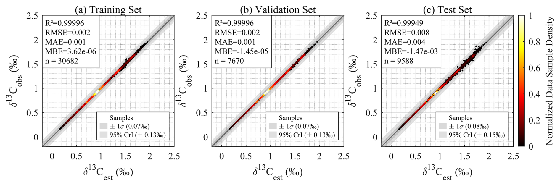
Figure A1 GPR model evaluation for numerical model δ¹³C_DIC reconstruction: Density scatter plots comparing GPR model-estimated (δ¹³C_est) versus numerical model outputs δ¹³C_DIC (δ¹³C_obs) values during (a) training, (b) validation, and (c) independent testing.

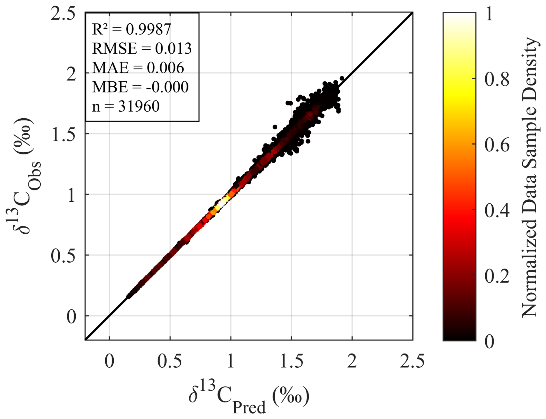
Figure A2 Density scatter plot comparing numerical model outputs δ¹³C_DIC (δ¹³C_Obs) versus predicted δ¹³C_DIC (δ¹³C_Pred) values.

This model-based validation complements the observational validation by addressing two critical limitations of sparse, uneven coverage data. The exceptional performance (R²>0.99, RMSE < 0.015 ‰) confirms that the GPR model can accurately reconstruct 4D δ¹³C_DIC patterns, validating its performance. In the meantime, meaningful anomaly-based R² values ranging from 0.67 to 0.90 validate the model's capacity to capture ecologically and biogeochemically relevant variations beyond simply reproducing large-scale background trends. This validation strengthens confidence that the reconstructed dataset is not constrained by methodological flaws. Instead, its limitations stem from inherent observational uncertainties such as sparse sampling and unmodeled biogeochemical variability, ensuring the dataset reliably captures the spatial-temporal dynamics of δ¹³C_DIC in the Atlantic Ocean.

A2 Observation-constrained Sparse Sampling Validation (Real-world Observational Scenario)

A2.1 Experimental Design Aligned with In-situ Observational Framework

To further enhance the credibility of the GPR model and the reconstructed dataset, and to address the concern that idealized grid-based subsampling may not fully reflect real-world observational scenarios, we supplemented an additional model-based validation that strictly mimics the spatial-temporal characteristics of sparse oceanographic observations. This validation focuses on evaluating the model's ability to learn from observation-like sparse data and generalize to target locations (e.g., GLODAP sampling locations), which is directly aligned with the core application scenario of the main text's δ¹³C_DIC reconstruction work.

The validation design strictly follows the real observational framework: (1) We subsampled the Claret et al. (2021) model data exclusively at the exact spatial locations of the 37 Atlantic cruises used in the main text's training, validation, and test sets, as well as the GLODAP sampling locations employed for prediction. Given that the model data only spans 1990–2002, we mapped observational data from other decades (e.g., 2000–2009 observations to 1990–1999 model data) to maintain a sample size comparable to the full observational dataset. This design exactly replicates the sparse, heterogeneous distribution of real oceanographic observations, eliminating the idealized grid-based subsampling bias. (2) The GPR model adopted the same parameter settings as the aforementioned grid-based validation, ensuring consistency and comparability of results across different validation scenarios.

A2.2 Model Configuration and Evaluation Metrics

Consistent with the previous validation, we used R², RMSE, MAE and MBE to assess the accuracy of point predictions for the training, validation, and independent test sets. For the GLODAP location prediction phase, we additionally performed Gaussian kernel density estimation (KDE) to evaluate the statistical congruence between reconstructed and native model δ¹³C_DIC distributions.

A2.3 Validation Results

The results of this observation-constrained sparse validation demonstrate robust performance of the GPR model (Fig. A3). The training set achieves an R² of 0.999 and an RMSE of 0.009 ‰, the validation set shows an R² of 0.9985 and an RMSE of 0.012 ‰ , and the independent test set yields an R² of 0.9950 and an RMSE of 0.025 ‰. These metrics confirm that the model can learn robustly from sparse, observation-like data and generalize effectively to unseen cruises, which is consistent with the performance of the grid-based validation and further verifies the model's stability.

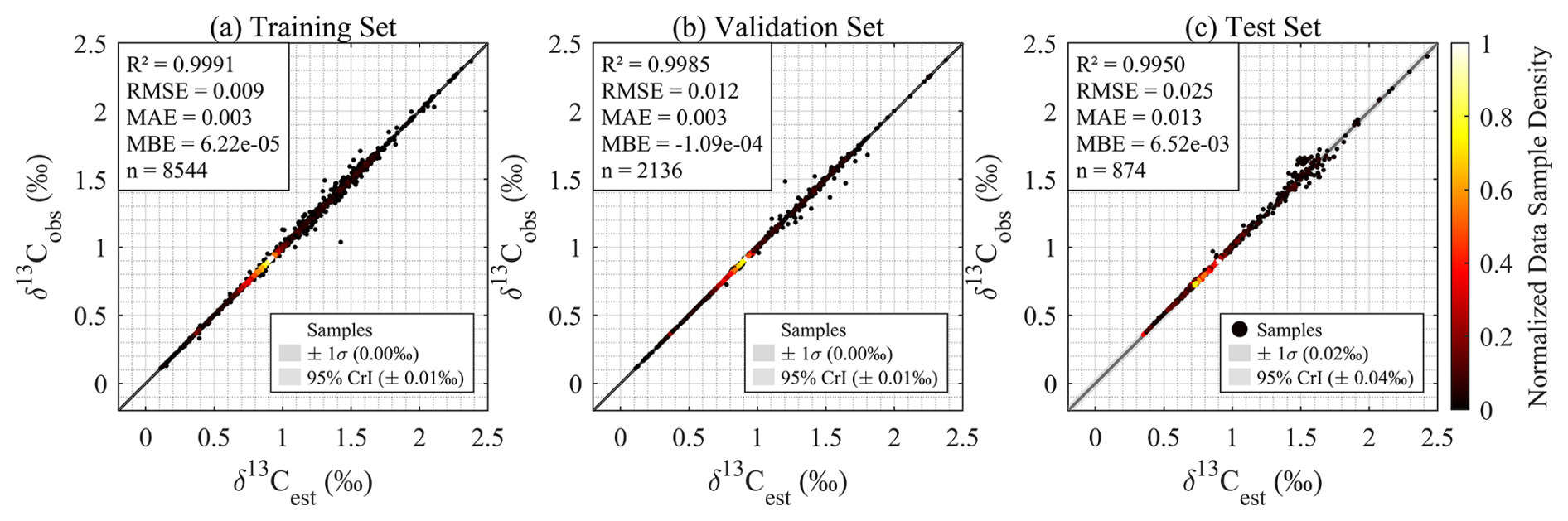
Figure A3 GPR model evaluation for numerical model δ¹³C_DIC reconstruction (observation-constrained sparse sampling): Density scatter plots comparing GPR model-estimated (δ¹³C_est) versus numerical model outputs δ¹³C_DIC (δ¹³C_obs) values during (a) training, (b) validation, and (c) independent testing.

For the prediction phase at GLODAP locations (Fig. A4), the reconstructed δ¹³C_DIC values align closely with the model's native values, with an R² of 0.95 and an RMSE of 0.080 ‰. High-density data points cluster tightly along the 1:1 line (Fig. A4a), indicating excellent consistency between the reconstructed results and the true model values. Some minor deviations from the 1:1 line are likely attributed to inherent uncertainties and biases in the numerical model itself, rather than the GPR model's performance. The KDE analysis (Fig. A4b) further underscores the strong statistical congruence between the numerical model δ¹³C values and the reconstructed estimates, with minor differences being negligible relative to the model's success in replicating the core characteristics of the native distribution.

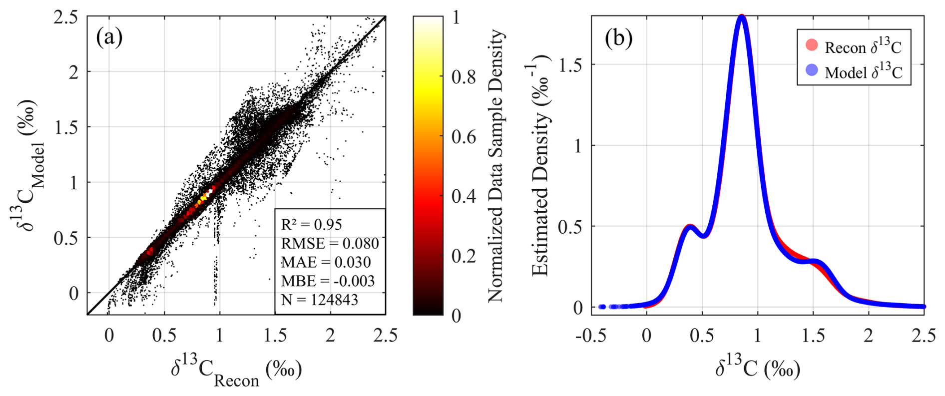
Figure A4 Comparison of model and reconstructed δ¹³C values at GLODAP locations (observation-constrained sparse sampling): (a) Density scatter plot of model versus reconstructed δ¹³C values (n=124 843). (b) Gaussian kernel density estimations (KDEs) for a comprehensive evaluation of model and reconstructed δ¹³CDIC values.

A3 Supplementary Full Atlantic Domain Generalization Test

To further verify the GPR model's ability to reproduce the full spatial-temporal distribution of δ¹³C_DIC across the entire Atlantic Ocean, we conducted a supplementary full-domain generalization test using the Claret et al. (2021) model data. Given the high computational memory demand of the original 1° × 1° horizontal resolution, 50 vertical levels full-domain dataset, we applied a sparse sampling strategy to maintain computational feasibility: we subsampled every other grid point in both the horizontal and vertical dimensions, and focused on the 1990–1999 period (120 months) for this test.

We used the identical GPR model trained on the observation-matched model data (Sect. A2), and predicted gridded δ¹³C_DIC values across the entire Atlantic domain, then compared these predictions to the model's native “true” δ¹³C_DIC values. The results show strong overall alignment between the reconstructed and native model values (Fig. A5), with an R² of 0.8305, an RMSE of 0.193 ‰, an MAE of 0.074 ‰, and an MBE of −0.024 ‰ across 8 425 440 valid samples. High-density data points cluster tightly along the 1:1 line, confirming that the model can reliably reproduce the large-scale spatial-temporal patterns of δ¹³C_DIC across the full Atlantic domain, and further demonstrating the model's strong generalization ability beyond the validation subsets.

This test provides additional evidence that our approach can effectively leverage sparse in-situ observations to estimate large-scale oceanographic δ¹³C_DIC distributions. Limited by current computational capability, this test is a preliminary assessment of full-domain generalization performance; more comprehensive optimization and in-depth analysis of full-basin reconstruction will be conducted in future work.

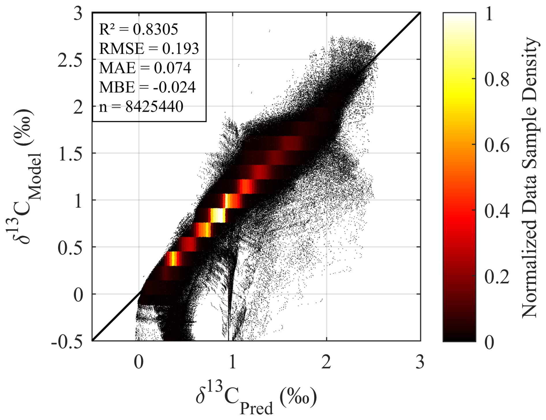
Figure A5 Density scatter plot of native model versus reconstructed δ¹³C_DIC values for the full Atlantic domain prediction phase.

A4 Conclusions of the Dual Validation Framework

This supplementary observation-constrained validation complements the previous grid-based validation, jointly reinforcing the reliability of the GPR model and the reconstructed data from two dimensions: “idealized grid sparse scenario” and “real observational sparse scenario”. The consistent excellent performance across both validation frameworks confirms that the GPR model can not only accurately reconstruct δ¹³C_DIC patterns from sparse grid data but also reliably learn from real-world sparse observational data and generalize to target application locations. This dual validation provides solid methodological support for the rigor of the main text's δ¹³C_DIC reconstruction work, further confirming that the reconstructed dataset can effectively address the limitations of sparse observational data and meet the needs of Atlantic carbon cycle research.