Advancing turbulence essential ocean variable: a reference glider-based microstructure dataset from the Western Mediterranean

We present a comprehensive dataset of turbulence microstructure measurements collected with a Micro Rider (MR-1000) from Rockland Scientific (RS) mounted on the Slocum Deep Glider “Teresa” across repeated transects between Sardinia and the Balearic Islands (SMART missions, 2015–2024) (https://doi.org/10.17882/107995, Kokoszka et al., 2025) This dataset constitutes one of the most extensive autonomous glider-based microstructure archives to date for the Western Mediterranean, containing glider sections up to 1000 m-depth and delivering quality-controlled vertical profiles of turbulent kinetic energy dissipation rate (ε) and thermal variance dissipation rate (χ) across seasonal cycles and diverse water masses. The data were processed through a rigorous multilevel workflow (L0–L4), following community best practices for processing, quality control, and uncertainty quantification. Final products include estimates of ε from dual shear probes and χ from dual fast thermistor probes, aligned with co-located hydrographic and oxygen measurements. This dataset provides a high-resolution resource for investigating fine-scale mixing, validating parameterizations, improving turbulence representation in models, and modeling physical processes. All data and processing codes are openly provided to support reuse, reproducibility, and integration into global efforts advancing the inclusion of turbulence as an Essential Ocean Variable.

1 Introduction

Starting from 2015, CNR-ISMAR in collaboration with Balearic Islands Coastal Observing and Forecasting System (SOCIB, Tintoré et al., 2013) set up a recurrent Slocum Deep Glider G2 mission along a longitudinal transect between the Sardinia (Italy) and the Balearic Islands (Spain), in the western Mediterranean Sea, called SMART (Sardinia MAllorca Repeated Transect). With the aim of monitoring water masses changes over the recent years and integrating the existing distributed multiplatform observing system in the Western Mediterranean Sea (Tintoré et al., 2019  Juza et al., 2025), the transect is also included in the Ocean Glider Program (Testor et al., 2019). Several water masses are present in the study area which allowed us to characterize their temporal and spatial variability. In the surface layers (0–150 m), Atlantic Water (AW) enters through the Strait of Gibraltar and undergoes progressive salinification as it circulates eastward and cyclonically through the western basin; below, the EIW core (200–600 m), characterized by salinities > 38.50 PSU and temperatures ∼ 13.3 °C, flows northwestward from the Eastern Basin and interacts with locally formed Western Intermediate Water (WIW) in winter, while the operation depth of the glider down to 1000 m allows to capture partially the upper part of the Western Mediterranean Deep Water (WMDW) (acronyms follow Schroeder et al., 2024). Such repeated missions are designed to characterize water mass properties and mixing/turbulence levels from seasonal to interannual scale.

In addition to the classical “conductivity-temperature-depth” (CTD) package, high-precision turbulence measurements are obtained through shear sensors and high-frequency thermistors installed on the Micro Rider (MR) from Rockland Scientific (RS). Over the past decade, the use of turbulence microstructure sensors mounted on autonomous platforms has significantly expanded the observational capacity of oceanographers to measure routinely small-scale mixing processes, using high-resolution measurements from shear and fast response thermistor sensors, to obtain respectively turbulent kinetic energy dissipation rate (ε, W kg⁻¹) and thermal variance dissipation rate (χ, °C² s⁻¹), over long-duration missions across various ocean regions (Eriksen et al., 2001; Wolk et al., 2009; Peterson and Fer, 2014; St. Laurent and Merrifield, 2017). While earlier deployments focused on pilot missions or single-process studies, few long-term, multi-season datasets from gliders exist, especially in the Mediterranean Sea environments. The present work provides one of the most extensive glider-based microstructure datasets to date for the Western Mediterranean. Collected from repeated transects between Sardinia and the Balearic Islands among nearly a decade, this dataset uniquely resolves ε and χ across key water masses and seasons (Kokoszka et al., 2025), complementing ship-based efforts and contributing to the broader goals of initiatives such as ATOMIX (Fer et al., 2024). The inclusion of processed data together with open-source processing code and rigorous quality control, ensures transparency, reusability, and relevance to multiple disciplines. This dataset thus represents a significant step forward in establishing turbulence from pilot (Le Boyer et al., 2023) to operational Essential Ocean Variable (EOV), addressing a long-standing observational gap and offering a benchmark for future observational and modeling studies.

In terms of region of interest, the western Mediterranean Sea serves as a crossroads for oceanic processes that influence regional and basin-scale circulation, water mass transformation, and ecosystem dynamics. The study area, situated between the Balearic Islands and Sardinia (Fig. 1), encompasses a complex transitional zone where Atlantic and Mediterranean water masses interact, mesoscale features dominate surface dynamics, and intermediate/deep flows modulate vertical exchanges. This region acts as a nexus for the convergence of multiple circulation systems, including the meandering eastward-flowing Algerian Current, the cyclonic Balearic Current, and the west- and northward propagation of the EIW. These interconnected processes make the Balearic-Sardinia corridor a strategic location for investigating the mechanisms governing heat, salt, and biogeochemical fluxes in the Mediterranean.

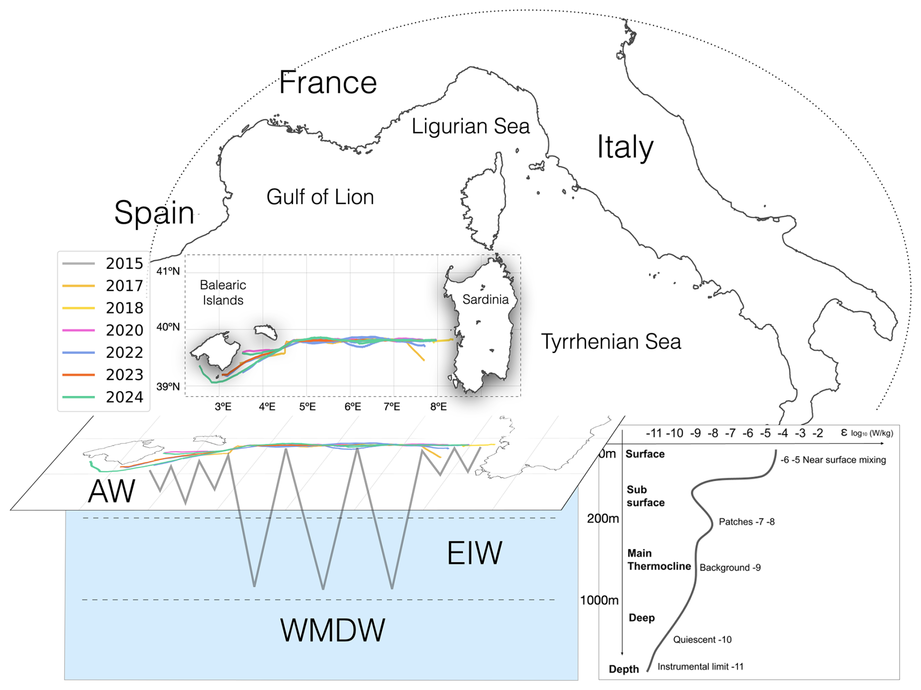
Figure 1 Glider Teresa mission along its longitudinal transect, by years (in colors). The scheme indicates the deployment between Sardinia and Balearic Islands in the Western Mediterranean Sea. Sawtooth black lines indicate a schematic trajectory from surface up to 1000 m-depth, encountering layers of the Atlantic Water (AW) in surface, the Eastern Intermediate Water (EIW) and the Western Mediterranean Deep Water (WMDW). Depth levels associated to these water masses (respectively 0–200 m, 200–1000 m, 1000 m+) are indicative. The lower-right panel provides a schematic representation of typical ranges of turbulent kinetic energy dissipation rates (ε, logarithmic scale) as a function of depth.

The circulation framework of this region has been described in several foundational studies of the western Mediterranean, which highlight the role of interconnected currents, boundary exchanges, and water-mass transformations linking the Balearic and Sardinian sub-basins (Millot, 1999; Send et al., 1999; Pinardi et al., 2015). The region exhibits intense mesoscale variability driven by the instability of the Algerian Current, which generates anticyclonic eddies that propagate into the study area (e.g., Testor et al., 2005; Aulicino et al., 2018). The bathymetry along the transect is predominantly uniform, with depths around 2500 m, except near the deployment ends where the continental shelves of Sardinia and the Balearic Islands cause shallower topography. Despite its dynamical importance, the Balearic–Sardinia section remained under-sampled due to logistical challenges and the transient nature of its key processes. The MOOSE GE cruises (Testor et al., 2010) that are carried out at annual frequency do not reach the section. Furthermore, these existing hydrographic campaigns provided snapshots but lack the spatial and temporal resolution to capture (i) diurnal-to-seasonal variability in EIW-WIW-WMDW interactions, which may play a role in regulating deep water formation in the Gulf of Lion, (ii) eddy-mediated cross-frontal exchanges that drive subsurface nutrient fluxes to Sardinia's oligotrophic shelf, (iii) responses to climate-driven perturbations, including, e.g., EIW warming and salinification (Schroeder et al., 2016; Testor et al., 2018; Margirier et al., 2020; Chiggiato et al., 2023). A sustained glider transect across this region offers unprecedented capabilities to quantify variations in water mass properties and transport using CTD, dissolved oxygen and microstructure profiles, enabling process-oriented oceanography.

Oceanic turbulent kinetic energy dissipation rates (ε) span over nine orders of magnitude with depth, as schematized in Fig. 1. Typical dissipation levels range from enhanced near-surface mixing ($\mathit{\epsilon }\approx {\mathrm{10}}^{-\mathrm{6}}$–10⁻⁵W kg⁻¹), to intermittent subsurface patches ($\mathit{\epsilon }\approx {\mathrm{10}}^{-\mathrm{7}}$–10⁻⁸ W kg⁻¹), background thermocline values ($\mathit{\epsilon }\approx {\mathrm{10}}^{-\mathrm{9}}$ W kg⁻¹), and increasingly quiescent deep waters approaching the instrumental detection limit ($\mathit{\epsilon }\approx {\mathrm{10}}^{-\mathrm{10}}$–10⁻¹¹ W kg⁻¹). These ranges are consistent with canonical dissipation levels reported in ocean mixing studies and widely used in vertical mixing parameterizations (e.g., Gregg, 1989; Waterhouse et al., 2014). A similar order-of-magnitude range applies to the thermal variance dissipation rate χ (not shown). Autonomous underwater gliders equipped with airfoil shear probes and fast-response thermistors enable concurrent estimates of ε and χ across a wide range of magnitudes during multi-week missions, providing vertically resolved observations of mechanical and thermal mixing beyond the capabilities of traditional ship-based profilers (Sherman and Davis, 1995; Eriksen et al., 2001; Peterson and Fer, 2014). Because turbulent mixing controls vertical exchanges of heat, salt, nutrients, and carbon, ε and χ are increasingly recognized as key parameters for sustained ocean observing systems and are currently considered emerging (pilot) Essential Ocean Variables (Lindstrom et al., 2012; Le Boyer et al., 2023; https://goosocean.org/what-we-do/framework/essential-ocean-variables/, last access: 25 July 2025). Recent advances in autonomous platforms and in processing, calibration, quality control, and uncertainty estimation methodologies have made the systematic acquisition and dissemination of turbulence microstructure datasets feasible (Lueck et al., 2002, 2024; Piccolroaz et al., 2021), motivating the present data compilation and its alignment with FAIR practices and community standards such as ATOMIX (Fer et al., 2024).

The dataset comprises seven mission-years (2015, 2017, 2018, 2020, 2022, 2023, 2024), ranging from one to over three months of data acquisition per year, and covering different seasons (2024: 21 May to 4 July; 2023: 27 June to 15 August; 2022: 9 September to 12 December; 2020: 2 March to 5 April; 2018: 23t April to 31 May; 2017: 6 to 26 April; 2015: 6 July to 18 August). While the glider missions were routinely conducted and monitored through standard CTD and navigation data, the turbulence microstructure dataset itself remained largely unexplored until this current compilation. As a result, several sensor limitations and data quality issues, affecting early missions went previously undetected. Over time, the acquisition setup and data handling improved significantly, with the period 2020–2024 representing the most consistent and quality-assured segment of the dataset. Earlier missions (2015, 2017) reflect an initial phase of setup and testing, while 2018 data remain excluded due to unrelated technical limitations. The Teresa's dataset consists of a large data ensemble, that once decomposed in continuous sections provides 3446 unique downward or upward gliding profiles across the upper layers of the Western Mediterranean Sea. The general processing choices that we will detail hereafter allowed us to obtain O(10⁵) valid estimates of ε and χ after quality control, on a vertical grid of around 1.5 m. This provides a rich and multi-purpose data set to be exploited at the crossroad of various important scientific questions from small scales processes to larger-scale variability, in a zone of interest reputed to intercept mesoscale fronts, latitudinal water masses exports, and deep winter convection.

2 Data and methods

2.1 Microstructure and glider data

Level 0 (L0) data consist of raw, high-frequency time series recorded by the MicroRider prior to any processing or spectral transformation. Shear and thermistor sensors provide turbulence measurements sampled at 512 Hz, which are internally logged by the Rockland MicroRider (model 1000-LP), a microstructure module designed for deployment on moving and fixed platforms such as gliders, moorings, or wire walkers. The instrument hosts two orthogonally oriented shear probes (sh1, sh2) mounted on the front bulkhead, measuring the vertical gradients of the horizontal velocity fluctuations, $\frac{\partial u^{\prime }}{\partial z}$, $\frac{\partial v^{\prime }}{\partial z}$ where the prime denotes deviations from the mean flow. Two fast-response FP07 thermistors similarly resolve small-scale vertical temperature gradients $\frac{\partial T^{\prime }}{\partial z}$. These sensors capture variance at spatial scales ranging from centimeters to decimeters, where turbulent motions are energetic, down to millimeter scales where viscosity will act to finally dissipate kinetic energy. In addition, the MicroRider includes a pair of piezo-accelerometers to monitor platform vibrations and a two-axis inclinometer providing pitch and roll angles with a nominal accuracy of 0.1°, allowing characterization of instrument dynamics during flight. For reliable shear-based turbulence measurements, the glider incident speed is expected to remain within approximately 0.2–0.6 m s⁻¹, fast enough to satisfy Taylor's frozen-turbulence hypothesis while slow enough to resolve the highest wavenumbers. Subsequent processing steps, including spectral analysis and dissipation estimation, are described in the following processing section.

While not strictly required for velocity estimation, we exploit the glider's dataset to geolocate the turbulence observations collected by the MR and to compute the instantaneous profiling speed required for converting shear probe signals into physical dissipation units. We apply the Glider Flight Model (GFM) from Merckelbach et al. (2019) to establish the glider incident velocity and angle of attack, used to improve the data conversion (RS Technical Note 039), and the overall turbulent estimates accuracy and further quality control. Processing turbulence data from gliders presents a significant challenge due to the size and complexity of the raw datasets. A single Level 0 file can contain sequences of 2 to 10 or more consecutive upward and downward gliding profiles, each spanning depths from the surface down to 1000 m. These profiles typically represent 10 to 12 h of continuous acquisition, resulting in file sizes that can reach up to 1 GB per file for deep glides. Estimating dissipation rates relies on spectral segmentation and windowing. Spectra are computed for each segment and subsequently combined, yielding an effective vertical resolution on the order of 1.5 m. This processing step substantially reduces data volume, with final profile products typically ranging between 1 and 10 MB per file. Nevertheless, the initial data volume imposes strict constraints on memory handling, processing time, and storage strategy throughout the workflow.

2.2 Turbulent dissipation rates

Microscale turbulence observations enable estimation of key quantities describing ocean mixing. ε is established from shear fluctuations as in Eq. (1):

$$\begin{array}{}\text{(1)}& \mathit{\epsilon }={\displaystyle \frac{\mathrm{15}}{\mathrm{2}}}\mathit{\nu }〈{\left({\displaystyle \frac{\partial u^{\prime }}{\partial z}}\right)}^{\mathrm{2}}〉={\displaystyle \frac{\mathrm{15}}{\mathrm{2}}}\mathit{\nu }\underset{\mathrm{0}}{\overset{\mathrm{\infty }}{\int }}{\mathit{\psi }}_{\mathrm{s}}\left(k\right)\mathrm{d}k\end{array}$$

where ν is the kinematic viscosity of water, and $〈{\left(\frac{\partial u^{\prime }}{\partial z}\right)}^{\mathrm{2}}〉$ is the variance of the velocity shear fluctuations, the brackets indicate averaging over a uniform turbulent collection. Here ψ_s(k) is the wavenumber spectrum, k the wavenumber (cpm), related to the frequency f (s⁻¹) through the profiling speed W (m s⁻¹) as $k=\frac{f}{W}$. Due to non-turbulent variance and electronic noise present in the signal, spectra are integrated over a restricted wavenumber range where turbulent variance dominates above the instrument noise floor. For shear-derived dissipation, the well-resolved portion of the shear spectrum is fitted to the reference empirical spectrum (Nasmyth, 1970; Osborn and Crawford, 1980; and in our case Lueck et al., 2002), and the fit is used to correct for unresolved variance outside the integration limits. Dissipation rates ε₁ and ε₂ are obtained independently from shear probes sh1 and sh2.

Similarly, χ is determined as in Eq. (2):

$$\begin{array}{}\text{(2)}& \mathit{\chi }=\mathrm{6}{\mathit{\kappa }}_{\mathrm{T}}〈{\left({\displaystyle \frac{\partial T^{\prime }}{\partial x}}\right)}^{\mathrm{2}}〉=\mathrm{6}{\mathit{\kappa }}_{\mathrm{T}}\underset{\mathrm{0}}{\overset{\mathrm{\infty }}{\int }}{\mathit{\psi }}_{\mathrm{T}}\left(k\right)\end{array}$$

where κ_T is the molecular thermal diffusivity and $〈{\left(\frac{\partial T^{\prime }}{\partial z}\right)}^{\mathrm{2}}〉$ the temperature gradient variance resolved by the FP07 thermistor and ψ_T is the temperature gradient (wavenumber) spectrum, for which theoretical models were proposed in Batchelor (1959) and Kraichnan (1968) spectra. Note that once χ is estimated, an associated ε_T can be derived indirectly applying ${\mathit{\epsilon }}_T=\mathit{\nu }{\mathit{\kappa }}_{\mathrm{T}}^{\mathrm{2}}(\mathrm{2}\mathit{\pi }{k}_{\mathrm{B}}{)}^{\mathrm{4}}$ with k_B is the Batchelor wavenumber established during the spectral fit. Spectral models, wavenumber ranges, and fitting procedures are described in detail in Lueck et al. (2024) and Piccolroaz et al. (2021), respectively, for shears and temperature.

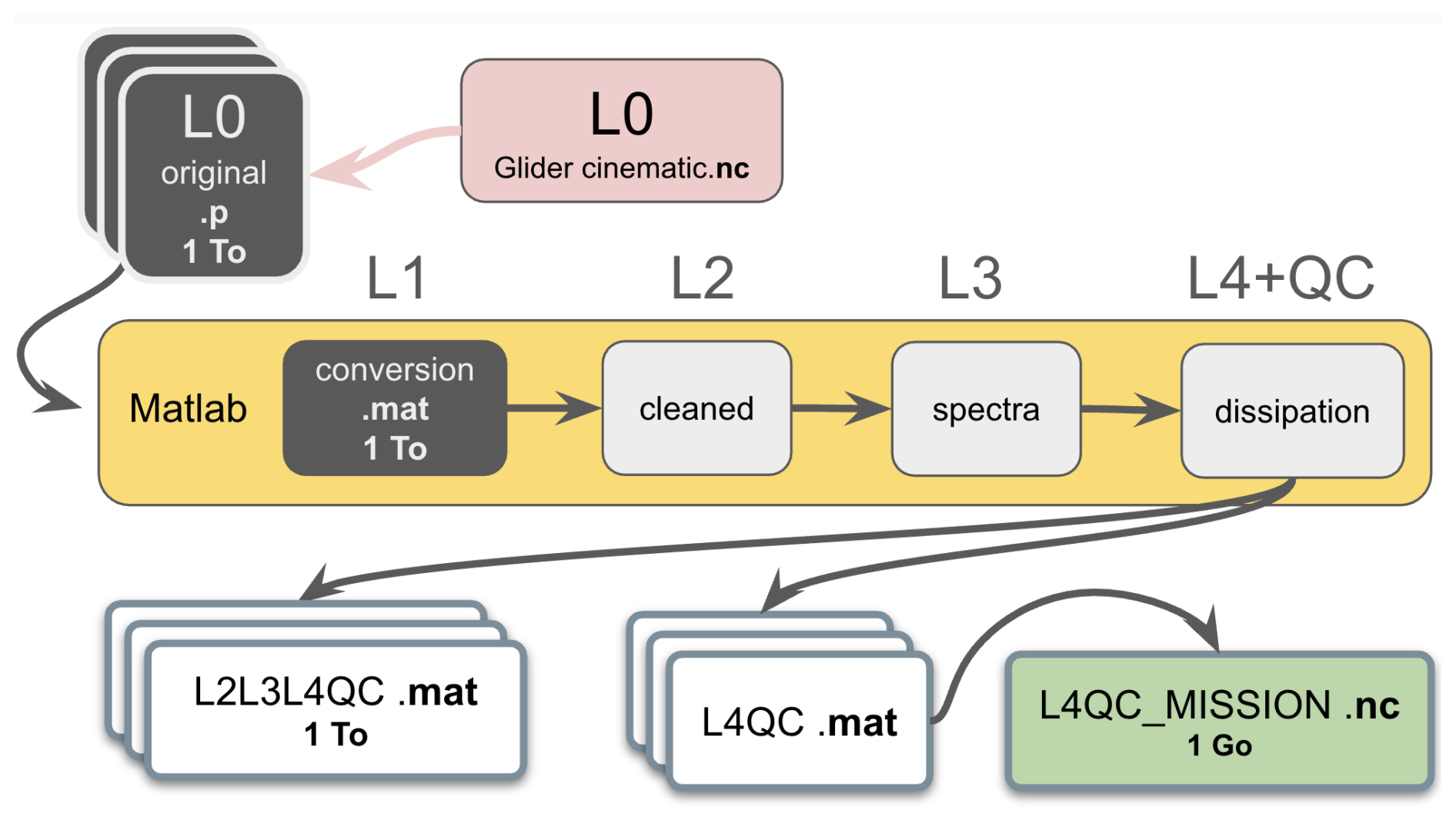
2.3 Processing flow and dataset available

The overall processing workflow follows the methodology described in Lueck et al. (2024), including spectral segmentation, noise-floor treatment, model fitting, and quality-control procedures, and is summarized in Fig. 2. We begin with retrieving, archiving, organizing, and listing original data files in directories (Level 0), followed by converting raw data into physical units (Level 1), cleaning and segmenting the time series (Level 2), generating wavenumber spectra from processed sections (Level 3), and finally estimating dissipation rates with quality control metrics (Level 4). These processing levels are designed to standardize the handling of microstructure data and ensure transparency in data processing. Each level builds upon the previous one, adding value and usability to the dataset. By the time data reach L4, they are labeled with a quality control flag, i.e., suitable for addressing complex scientific questions about ocean mixing processes. The dataset published here corresponds to Level 4 data (quality-controlled and validated). Raw and intermediate processing levels (L0–L3) are not included in this publication due to their large volume. Once reached the L4 level, data is exported to a netCDF file (in green on the Fig. 2) with an additional list of metadata. The dataset we propose is available at: https://www.seanoe.org/data/00968/107995/ (last access: 28 July 2025, https://doi.org/10.17882/107995, Kokoszka et al., 2025). It consists of a unique netCDF “TERESA_MR_SMART_MISSIONS_2015_2024_L4_QC.nc” including the missions from the years 2015 to 2024.

Figure 2 Scheme of the processing steps along the various levels.

3 Processing

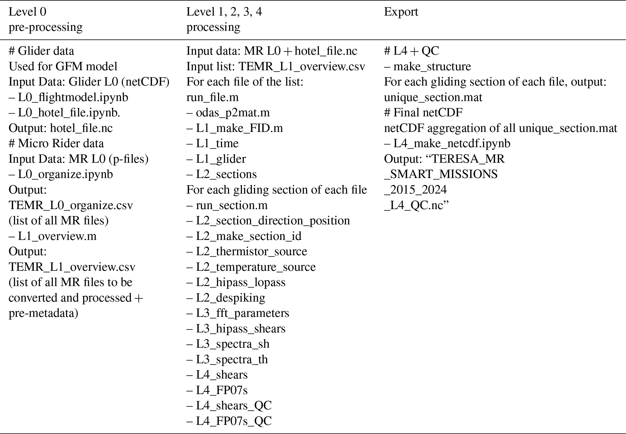
All processing routines used in this study are made available (https://doi.org/10.5281/zenodo.16541936, Kokoszka, 2025) and include Python notebooks and MATLAB scripts. The analysis relies on functions from the ODAS v4.51 MATLAB toolbox by RS for shear probe processing (Lueck et al., 2020), improved with methods outlined in Lueck et al. (2024), and MATLAB routines from Piccolroaz et al. (2021) for thermistor-based estimates. Routines used along the processing steps are synthesized in the Table 1, and then detailed in the following sections.

Table 1 Summary of the processing routines.

3.1 Pre-processing step – MicroRider data screening and Glider data merging

3.1.1 Glider data

To ensure the quality of turbulence estimates, a correct glider incident velocity must be provided and nested with the original microstructure data, to support the data conversion into physical units and to be used along the general processing. To achieve this, estimates of the glider's speed through water is calculated using the Glider Flight Model (GFM) from Merckelbach et al. (2019). The process employs the Level-0 glider data, available via SOCIB's Erddap/Thredds server (Chiggiato et al., 2021).

In the notebook L0_flightmodel.ipynb we load the deployment-specific netCDF file and extract the navigation and physical variables (timestamps, pressure, temperature, conductivity, pitch, roll, oil volume for buoyancy control, and GPS coordinates). The glider's pressure and position data provide a geographical context for the MR profiles, and glider's speed is reconstructed with the flight model using a physical balance between buoyancy, drag, and pitch (Merckelbach et al., 2019). Code for the model is provided by the authors (https://github.com/smerckel/gliderflight/tree/master, last access: 25 April 2025, https://gliderflight.readthedocs.io/en/latest/index.html, last access: 25 April 2025). Additionally, glider temperature will be exploited later as a calibrated reference to calculate the kinematic viscosity of seawater (see thereafter in Processing). Once all of these quantities are obtained, a unique hotel file in netCDF format is created with L0_hotel_file.ipynb. This is the auxiliary data file that supplies time-synchronized estimates of profiling speed and, and optionally, other dynamic parameters (e.g., angle of attack, pitch) that are not directly available or accurate enough in the raw microstructure data. This external input is particularly useful when the instrument is mounted on platforms such as gliders or AUVs, where the speed through water cannot be reliably estimated from pressure rate alone due to oblique motion or complex vehicle dynamics. An overview of velocities can be consulted in Fig. S1 in the Supplement. Extracted from the hotel, the GFM velocity will override the profiling speed that would be estimated by default from the MR pressure rate change and pitch if no externally computed velocity is provided. The speed is passed to odas_p2mat() via the convert_info.hotel_file argument in input of the function, and it is internally interpolated to the time base of the microstructure data.

3.1.2 MicroRider data screening and pre-load

Files are retrieved and organized in folders, and original raw data files from the MicroRider (.p-files) are listed with L0_organize.ipynb in a csv file named TEMR_L0_organize.csv. The following steps are then made using MATLAB scripts. The routine L1_overview.m performs a trial check of all listed L0 raw microstructure files, in preparation for L1 data conversion. For each file, it archives the embedded setup_cfg configuration file from the MR (which contains sensor-specific calibration coefficients and acquisition settings), and if needed, replaces it with an updated version to correct inconsistencies in early mission years. It then integrates the external hotel file containing glider data to be nested for data conversion and processing. The script eventually lists general metadata about files (e.g., size, path) and estimates the local time offset to reference glider and MR clocks. TEMR_L0_organize.csv is completed and exported as TEMR_L1_overview.csv that will serve for the processing run. This pre-procedure provides a screening step anticipating the former L1 conversion, ensuring the input data is consistent, patched if necessary, and ready for accurate time-synchronized processing.

3.2 L1 – converted data

The master script run_file.m calls various sub-scripts (described thereafter) that are used to process a selected L0 raw data file from the screening list and perform L1 conversion, before splitting the data in convenient continuous gliding sections that initiate the L2 step. It starts by identifying the mission year and filename, then extract and archive the internal setup_cfg configuration file. For data collected in or before 2022, it replaces the configuration with an updated version (setup_216_corrected.cfg) to correct known configuration issues. A structure variable (conversion_info) is declared, containing information for data conversion, including a pointer to the external hotel file, which provides synchronized glider speed and angle of attack. A time offset between glider and turbulence timestamps obtained at the pre-processing step is applied there and ensure time alignment. Data is converted from raw signal to physical units through odas_p2mat().m, supported by the glider's velocity provided by the hotel file. This glider velocity replaces the MR default speed (inferred from its own sensors alone). Any other variables nested into the hotel file are merged with the microstructure converted data and are made available as additional fields in the MATLAB data structure. A unique filename identifier  FID) is built for each converted file in L1_make_FID.m, combining mission metadata such as: glider name (TERESA), sensor type (MR), conversion level (L1_converted), internal file ID and original filename, date and time extracted from the data header. Time vectors are defined in L1_time.m for both slow and fast acquisition channels (sampling respectively at 64 and 512 Hz). It combines the starting timestamp (date, hour, minute, second, millisecond) with the elapsed time vectors t_fast and t_slow to produce MATLAB datetime and datenum arrays. If not already interpolated during the conversion, glider variables are interpolated in L1_glider.m on both fast and slow time stamp grids to be ready to use alongside the microstructure data. Key variables include angle of attack (AOA), pitch, roll, temperature, conductivity, salinity and density, kinematic viscosity, thermal diffusivity, and position (longitude and latitude).

3.3 L2 – unique gliding sections

At the end of run_file.m the script L2_sections.m serves as a transition between L1 and L2 levels. It segments time series into continuous unique gliding sections. For this, it employs pressure (P_fast) and vertical velocity (W_fast) in the function get_profile.m from ODAS. A low-pass Butterworth filter is first applied to W_fast using a cutoff frequency Fc equal to the mean glider speed. This suppresses high-frequency noise of the vertical velocity, which eases the detection of profiling starting and ending indices. A profile is accepted if it satisfies minimum conditions: Depth ≥ Pmin (e.g. 3 dbar); Vertical speed ≥ |Wmin| (e.g. 0.01 m s⁻¹); Duration ≥ minDuration (e.g. 60 s). The function detects down and upcasts and start and end indexes of each detected section are retained, and a unique integer label is assigned. Direction flags are also set (+1 for downcast, −1 for upcast). Once listed, unique gliding sections will be processed separately (i.e., in loop) and be passed through the sequence of scripts called on run_sections.m that we describe thereafter.

3.4 L2 – cleaning and processing

We identify in L2_section_direction_position.m the temporal extent and key navigation attributes, and we extract the section indices of the current gliding section. A unique identifier is created with L2_make_section_id.m. The routine considers the original file identification string defined at L1 and adds other strings suffixes from the values of the current section. The core identification is as follows, with XXX being named accordingly from the level of processing to be considered in case of data export (e.g., XXX = “L1”, “L2”, or “L1L2L3” etc.), if applicable: e.g., TERESA_MR_XXX_converted_file_0062_DAT_063_2024 _06_06_23_40_05. As we separate by unique section, we add: the position as: Lat, Lon lat_39_7987_lon_07_6116; Navigation: nav_E; Pmin, Pmax: pmin_0003_pmax_0954; Section number: sec_001; Section total: on_004; Gliding direction: glid_down. This convention produces long but robust and comprehensive filenames: TERESA_MR_XXX_converted_file_0062_DAT_063_2024 _06_06_23_40_05_lat_39_7987_lon_07_6116_nav_E_pmin _0003_pmax_0954_sec_001_on_004_glid_down.

The script L2_thermistor_source.m identifies the most reliable fast thermistor (FP07) to be used as the reference thermistor signal. It compares the two FP07 time series (T1_fast and T2_fast) against the glider's temperature (T_gl_slow, interpolated on the fast channel) by calculating the Pearson correlation coefficient (cc) between signals. If both sensors correlate significantly with the glider temperature (above a threshold, e.g., cc > 0.3), the one with the higher correlation is selected as the master one (flag 11 or 22). If only one meets the threshold, that sensor is chosen (flag 1 or 2). If none correlates significantly, the decision is made based on the variance of each FP07 channel, using a low-variance (stuck-sensor) test on the considered gliding section. If both variances are unusually below an empirically defined threshold of $\mathrm{1}\times {\mathrm{10}}^{-\mathrm{5}}$ °C², indicative of a stuck or flat-line thermistor signal, the function flags potential malfunction (flag 0); if only one is below, the other is selected (flag 100 or 200). In case both are above the variance threshold but do not correlate with T_gl_slow, the sensor with the lower variance is preferred (flag 10 or 20). The outcome is stored with a logical value and a string (thermistor_source). This step allows to track potential FP07 malfunctions. Note that a malfunctioning sensor will not pass the quality control applied later in L4.

L2_temperature_source.m defines the reference temperature profile used to compute the kinematic viscosity of seawater required for ε estimates. The selection is based on the Th_source_logic flag assigned during the thermistor comparison step. In the vast majority of cases (Th_source_logic = 11, 22, 1, 2, 0, 100, or 200), the glider temperature interpolated on the fast channel (T_gl_fast) is retained as the reference temperature. Cases where Th_source_logic equals 10 or 20, indicating that both FP07 thermistors exhibit sufficient variance but correlate poorly with the glider temperature, are rare. They represent about 2.3 % of the processed sections and 1.2 % of all dissipation estimates, and account for only 0.13 % of the fully validated (“QC = 0”) ε estimates. These occurrences are restricted to the earliest part of the dataset (year 2015). In such cases, the FP07 thermistor with the lower variance (T1_fast or T2_fast) is used instead of T_gl_fast. For these sections, the temperature offset between FP07 and glider measurements is typically on the order of ∼2 °C. Over the observed temperature range (approximately 10–20 °C), this translates into a change in kinematic viscosity of less than 4 %, which has a negligible impact on the resulting ε estimates compared to other sources of uncertainty. The selected signal is stored as temperature_for_dissipation together with a descriptive string and logic flag, and is used subsequently in get_diss_odas().

The script L2_hipass_lopass.m applies sequential high-pass and low-pass Butterworth filters to the shear probe signals (sh1, sh2). First, a high-pass filter with a cutoff frequency of 0.1 Hz is used to remove low-frequency trends and motion-related biases, preserving the turbulent fluctuations of interest. The absolute value of the high-passed signals is computed to obtain envelope-like signals (sh1hpa, sh2hpa). Then, a low-pass filter with a cutoff at 1 Hz is applied to smooth these envelope signals, yielding sh1hpalp and sh2hpalp to be conserved apart for other applications (e.g., visual check).

We perform through L2_despiking.m an automated spike detection and removal on the filtered shear signals (sh1hpa, sh2hpa) using a despiking algorithm. It applies the ODAS despike() function with a defined amplitude threshold (thresh = 8), a frequency cutoff (fcut = 0.5 Hz), and a smoothing window length ($N=\mathrm{0.04}\times \mathrm{Fs}$, with Fs = 512 Hz) to identify and suppress sharp, non-physical signal excursions. The outputs include the despiked shear signals (sh1hpa_dsp, sh2hpa_dsp), the spike indices, the number of iterations required to converge (pass_count), and the fraction of samples affected (ratio). Additionally, spike indices are conserved with their associated pressure levels (P_spikes_sh1, P_spikes_sh2) to flag and keep track of spike occurrences.

3.5 L3–L4 – spectral computation and turbulent estimates

Wavenumber spectra are calculated from the cleaned gliding sections obtained at the L2 step. We employ there the functions get_diss_odas() for shears, and gradT_dis_spec() for FP07, that do both spectral computation and integration to obtain ϵ and χ, respectively. Once calculated, the different outputs are organized through L3 and/or L4 products.

Dissipation rates of turbulent kinetic energy (ε) are estimated from shear probe data using spectral integration of the velocity gradient spectra, following the procedures described in Lueck et al. (2024). If ε exceeds $\sim {\mathrm{10}}^{-\mathrm{5}}$ W kg⁻¹, a transition is made from direct integration in the variance subrange (VSR) to inertial subrange (ISR) fitting, as spectral roll-off and probe resolution limit the reliability of the full-spectrum approach. Following Lueck et al. (2024), quality metrics that will be presented hereafter are calculated and allow to flag quality-controlled passing estimates.

For temperature microstructure, thermal variance dissipation rates (χ) are estimated from FP07 thermistor spectra following Piccolroaz et al. (2021). This includes correction for the sensor's finite time response, which acts as a low-pass filter and attenuates high-frequency content of the temperature gradient spectrum. The correction is based on profiler speed and the thermistor's thermal time constant (typically around 7 ms for FP07 sensors), and is applied through a transfer function modeled after the thermistor's response characteristics. Accurate χ estimation depends critically on this correction, especially in energetic conditions where high wavenumber contributions are significant. As with ε, χ estimates are quality controlled using statistical thresholds and consistency between the two independent FP07 thermistor-derived estimates. Each ε or χ estimate is accompanied by metadata including the wavenumber range of integration, spectral model used, uncertainty metrics (e.g., standard deviations from VSR or ISR methods), and a consolidated QC flag. At the end, if both sensors pass quality assurance, a strict final dissipation or thermal variance estimate is computed as the average across sensors.

We define in L3_fft_parameters.m the parameters for the Fast Fourier Transform (FFT). It starts by estimating the glider's mean speed (speed_mean) and vertical speed (w_mean) over the gliding section. The characteristic FFT window duration (tau_fft) is determined by the minimum of two criteria: (i) to avoid signal contamination from the 1.5 m vehicle-scale motions (vehicle_length/speed), and (ii) to resolve a spectral scale of 0.5 cpm. From this duration, the number of FFT points (N_fft) is computed using the sampling frequency, and the corresponding spatial window length (L_fft) is used to define the lowest resolved wavenumber (kl = 1/L_fft). The code also sets the high-pass frequency cutoff (Fhp). FFT spectra are first computed on short segments length (N_fft) of typically 3 s duration. Dissipation estimates are then obtained by averaging spectra over a longer window composed of Ntimes = 4 FFT segments, using a 50 % overlap between consecutive segments. This results in an effective averaging window of approximately 12 s and corresponds to averaging seven individual FFT spectra for each dissipation estimate.

In L3_hipass_shears.m, a 1st-order Butterworth high-pass filter is applied on shears (sh1hpa_dsp, sh2hpa_dsp) with a cutoff frequency (Fhp) derived in the FFT parameters, to remove low-frequency noise. The filtered shear are obtained using zero-phase filtering to prevent phase distortion.

Key parameters for the Fast Fourier Transform (FFT) are used to lead spectral dissipation estimation in L3_spectra_sh.m. The ODAS function get_diss_odas() computes the dissipation rate ϵ from the shear spectra. Vibration-induced noise from the glider platform and pump is filtered from the raw shear signals through the noise correction implemented in the ODAS v4.5.1 toolbox, which consist of removing coherent signals between the shears and vibration sensors (Ax, Ay) in the frequency domain, following Goodman et al. (2006). Profiles of dissipation rate (ε) are obtained then for each shear sensor.

Spectral analysis of temperature gradient is performed in L3_spectra_th.m using the gradT_dis_spec() routine from Piccolroaz et al. (2021) to estimate temperature variance dissipation rates (χ). Inputs include pressure, vertical temperature gradients ($\mathrm{d}T/\mathrm{d}z$), and required parameters such as the kinematic viscosity of seawater and spectral models. Segments of the temperature gradient signal are analyzed, and theoretical Batchelor or Kraichnan spectra are fitted to the observed spectra using a Maximum Likelihood Estimation (MLE) method following Ruddick et al. (2000). The MLE fit is used both to correct χ for unresolved variance outside the integration range and to provide an independent estimate of ε derived from temperature-gradient spectra, without using shear-derived ε as input. Quality metrics returned by the routine include the Mean Absolute Deviation (MAD), the wavenumber range used for the fit, likelihood ratios, and QC flags for spectral fits. Profiles of χ are obtained independently for each FP07 sensor. For enhanced turbulence levels, the downcast glider speed may limit the resolution of the high-wavenumber roll-off of the temperature-gradient spectra; in such cases, the reliability of χ and ε estimates is evaluated using the MLE-based quality metrics and associated QC flags.

Once the estimates are obtained, L4_shears.m collects the dissipation rate estimates together with their associated quality metrics and hydrological variables. It interpolates glider-derived variables (e.g., speed, temperature, salinity, density, pitch, roll, angle of attack) onto the time base of the estimates. Uncertainty estimates are obtained directly from the spectral fitting routine get_diss_odas() and stored to be employed thereafter. In L4_FP07s.m, the thermal variance dissipation rate (χ) estimates are extracted and compiled for output. It retrieves the associated pressure and depth vectors, timestamps, and positions.

3.6 L4 – Quality Control (QC)

A structured set of quality control (QC) is applied in L4_shears_QC.m and L4_FP07s_QC.m to the individual estimates, respectively (ε₁ ,ε₂) and (χ₁, χ₂). The QC flag for shear-derived ε is a single cumulative value that encodes the outcome of several individual quality tests, resumed in the Table 2: (1) Figure of Merit (FOM), which fails if the spectral fit exceeds a threshold (FOM > 1.4); (2) Spike Fraction, which flags data with more than 5 % of points removed during despiking; (4) Inter-Probe Epsilon Ratio, applied only if both probes have valid FOM, and flags significant disagreement between ε₁ and ε₂ (values out of 2.77×σ(ln  ε) for VSR; 4.2×σ(ln  ψ) for ISR, see Lueck et al., 2024); (8) Spike Iteration Count, which flags segments requiring more than 9 despiking passes; (16) Variance Resolution, which fails if less than 60 % of the shear spectrum variance is resolved; (32) Relaxed Spike Fraction, used to flag cases where spike fraction falls between 5 % and 15 %; (64) Method Mismatch, which flags segments in case of the two probes used different estimation methods (VSR or ISR) on the same data segment; (128) that flags angles of attack out of the range 1.5–4.5°. The final QC flag is a bitwise sum of failed tests. In the QC table, the failure condition “none” refers to an individual probe estimate for which no QC test has failed. All individual and inter-probe consistency checks (including ratio and method-consistency tests, flags 4 and 64) are applied at the probe level. As a result, inter-probe tests may reject only one of the two estimates (ε₁ or ε₂), while the other can remain valid.

Table 2 Summary of QC controls.

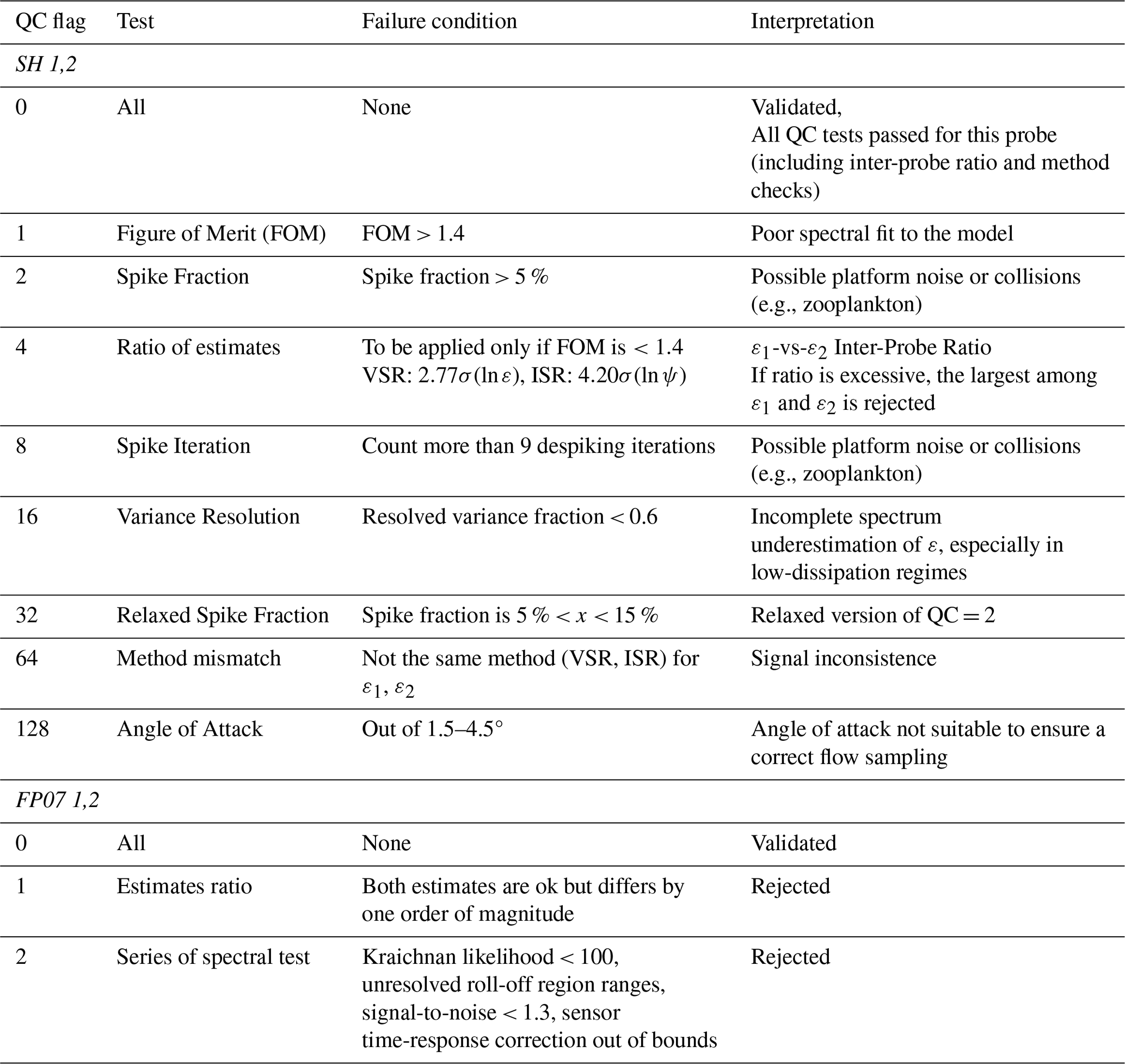
Although shear-derived ε estimates are available elsewhere in the dataset, they are not used to constrain χ estimation or the associated spectral QC, which relies exclusively on temperature-gradient MLE fits following Piccolroaz et al. (2021), and we employ the QC flag in output from their routines, that we conveniently reordered as (0) for good data, (1) if both estimates flags initially (0) but are separated by one order of magnitude in intensity when cross-checked, and (2) for poor estimate (e.g., bitwise sum, QC = 3 corresponds to 1+2). Note that in their routines the poor QC flag combines multiple spectral quality criteria into a single flag that we do not exploit separately, including: (i) the likelihood ratio (LR), requiring that the fit to the Kraichnan model significantly outperforms a power-law fit (LR > 100); (ii) the integration range criterion, ensuring that the spectral peak and roll-off are both resolved; (iii) a signal-to-noise ratio threshold, with SNR > 1.3 in the fitted spectral range; and (iv) the effect of the sensor time-response correction to avoid spectral distortion.

4 Data structure

4.1 Data structure and export

The script make_structure.m compiles metadata, processing parameters, quality-control diagnostics, and turbulence estimates into structured MATLAB files for each glider profile section. Two levels of data products are generated: a comprehensive internal structure containing all intermediate signals, spectra, and diagnostics, and a lighter structure retaining only essential metadata, processing parameters, final dissipation estimates (ε and χ), and QC flags. To balance data traceability with storage and computational constraints, only the lighter product is published, while the full structure is retained internally for reproducibility and potential reprocessing. Each section is exported as an individual .mat file using the -v7.3 format and named following a standardized convention encoding key metadata (mission, time, location, depth range, and glider direction, see Sect. S1 in the Supplement).

4.2 netCDF aggregation

We aggregate all the section data and metadata as variables and attributes into a netCDF file. It contains several groups of variables, organized in five different dimensions. Note that suffixes _SHEAR or _THERM serve to distinguish between the variables related to the shears or FP07s sensors, respectively. Here we give a generic example of dimensions in case of a vector of X shear-based estimates for 2 shear sensors, and Y thermistor-based estimates for 2 thermistor sensors, all obtained among Z unique sections among all the mission years:

• SECTION contains scalar values used for each individual section (e.g., processing parameters). Dimension is (Z, 1).

• TIME_SPECTRA_SHEAR serves to contain shear-related estimates. Dimension is (X, 1).

• TIME_SPECTRA_THERM serves to contain thermistor-related estimates. Dimension is (Y, 1).

• N_SHEAR_SENSORS. Dimension is (2, 1).

• N_THERM_SENSORS. Dimension is (2, 1).

Note that TIME_SPECTRA_SHEAR and TIME_SPECTRA_THERM are different given the two different spectral computations leading to slight variations in FFT lengths, and consequently on depth and timestamps associated to their respective estimates. They can be merged later, e.g. on the same depth/time grid, once the QC choices are made to filter out values. Variables and their dimensions are summarized in the Table 3.

Table 3 Overview of the variables made available in the netCDF file.

5 Results

5.1 QC for spikes and Figure of Merit (FOM)

We implemented quality control metrics related to despiking following the section-based approach described by Lueck et al. (2024). Despiking is applied to each gliding section prior to spectral analysis, and spike occurrences are identified during this step. In principle, the resulting spike indices can be used to compute spike fractions at the dissipation-length segment level. In the present processing, spike statistics are instead summarized at the section level and the corresponding QC flags are applied to the dissipation estimates derived from that section.

A spike fraction test assigns QC = 2 when more than 5,% of the clean section data points are affected by despiking. This flag indicates that core validation criteria – acceptable spectral fit, agreement between probes, and sufficient resolved variance – are satisfied, but that elevated spiking is present. Such cases are not necessarily invalid, as spikes may arise from dense biological layers, brief mechanical disturbances, or localized contamination superimposed on otherwise valid turbulent signals. A second despiking diagnostic assigns QC = 8 when more than nine despiking iterations are required. As noted by Lueck et al. (2024), there is no strong consensus on acceptable iteration limits, and ODAS processing caps the number of iterations by default, which limits the interpretive value of this metric alone.

Our statistical analysis (Fig. 3) reveals a subset of estimates with spike fractions between 5 % and 15 % and iteration counts below the rejection threshold. To avoid overly conservative rejection of such cases, we introduce a relaxed quality flag, QC = 32, marking these estimates as conditionally valid. For long glider profiles extending to 1000 m, localized spikes may occur without substantially affecting the overall spectral estimate. Applying a strict section-level rejection in these cases would unnecessarily reduce data availability. The QC = 32 flag therefore provides a practical compromise, retaining these estimates for secondary analyses while clearly identifying them as non-core data and leaving the final selection to the user.

Figure 3 Count of spiking fraction (a, b) and pass count (c, d) for shear 1 (blue) and shear 2 probes (red), by bins of glider depth extension, in meter (i.e. from short to long glide). Count of FOM values (e) for shear 1 (blue) and shear 2 (red).

The figure of merit (FOM), a key indicator of spectral fit quality, exhibits variability between probes. In our dataset, FOM values from shear probe sh2 distribute consistently around 1 (Fig. 3e), while sh1 presents a bimodal distribution centered near 1 and 1.4. Despite its frequent use, there is no universal consensus on an optimal figure-of-merit (FOM) threshold, as its interpretation depends on probe characteristics, platform type, and environmental conditions (Lueck et al., 2024). Following the guidance of Lueck et al. (2024), we adopt a nominal threshold of FOM = 1.4 as a practical limit, while acknowledging its subjective nature. Users of the dataset are encouraged to apply alternative FOM thresholds if more appropriate for their specific scientific objectives or observational context.

As such, in future applications or targeted analyses, a relaxed QC threshold could be considered. All dissipation estimates are published together with their associated QC flags, which explicitly document their quality status. This approach ensures transparency and allows users to apply their own selection criteria depending on their scientific objectives, while fully respecting the quality-control thresholds adopted in this dataset.

5.2 Representative examples of spectral quality control outcomes

Figure 4 illustrates representative examples of the spectral quality control applied to both shear- and thermistor-derived turbulence estimates. In validated cases (a, c), the observed spectra closely follow the theoretical reference models over a well-resolved wavenumber range, with consistent behavior between paired sensors and integration limits that avoid both low-wavenumber contamination and high-wavenumber noise. These conditions yield stable and comparable estimates of ε (shear) and χ (thermistors).

Figure 4 Examples of shear- and thermistor-based spectra illustrating accepted and rejected estimates. Panels (a, b) show shear cases and panels (c, d) thermistor cases. Left subpanels display the raw and retained signals (sh1 in blue, sh2 in red; th1 in blue, th2 in red; glider temperature in black for thermistors) over the dissipation segment. Right subpanels show the corresponding wavenumber spectra. For shear, observed spectra are compared to the Nasmyth model; for thermistors, to the Kraichnan model. Dashed curves indicate the fitted reference spectra; symbols mark the spectral integration limits used to compute ε or χ. Panel (a) (23 May 2024) illustrates a fully validated shear case (QC = 0–0). Panel (b) (22 May 2024) shows a shear case rejected due to poor spectral fit (QC = 1–1; elevated FOM). Panel (c) (12 September 2022) presents a validated thermistor case (QC = 0–0). Panel (d) (15 March 2020) shows a thermistor case where one probe fails QC while the other remains acceptable (QC = 1–3).

Rejected cases (b, d) highlight the main failure modes identified by the QC framework. For shear (b), large deviations from the Nasmyth spectrum at intermediate wavenumbers lead to elevated figures of merit and inconsistent estimates between probes. For thermistors (d), one probe exhibits excess variance and poor agreement with the Kraichnan fit, while the companion probe remains usable, resulting in asymmetric QC flags. Together, these examples demonstrate how the combined use of spectral shape, model fit quality, and inter-sensor consistency discriminates robust turbulence estimates from those affected by noise, platform dynamics, or sensor degradation.

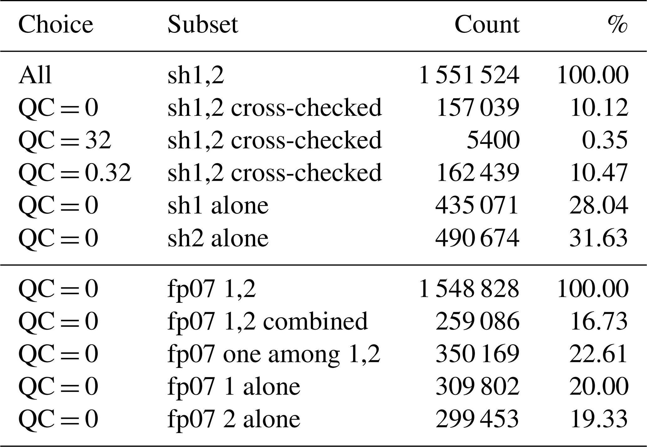
5.3 QC counting

Figure 5 presents the cross check of shear-based and thermistor-based estimates. We present in Fig. 6 the counting of all unique tests we performed on the data (and detailed in Table 4). If counting the strict cross-checked cases when both sensors of shear and thermistor pass QC = 0, around 10 % of good estimates remain for shears, against 16 % for thermistor. Employed singularly, sensors reach 28 % and 31 % for shear 1 and 2, respectively, and 19 % and 20 % for FP07 1 and 2, respectively. These estimates alone are less affitable than the cross-checked but can be employed with caution by the user in a contextual use. The low proportion of cross-validated estimates primarily reflects sensor degradation during deployments and variable glider flight conditions, rather than a lack of usable individual measurements.

Figure 5 Scatter plots of cross-checked estimates of (ε₁, ε₂) and (χ₁, χ₂). Gray points indicate all estimates; (a) green indicates the (best) cross-probe choice; (b) yellow indicates that both FP07 estimates pass.

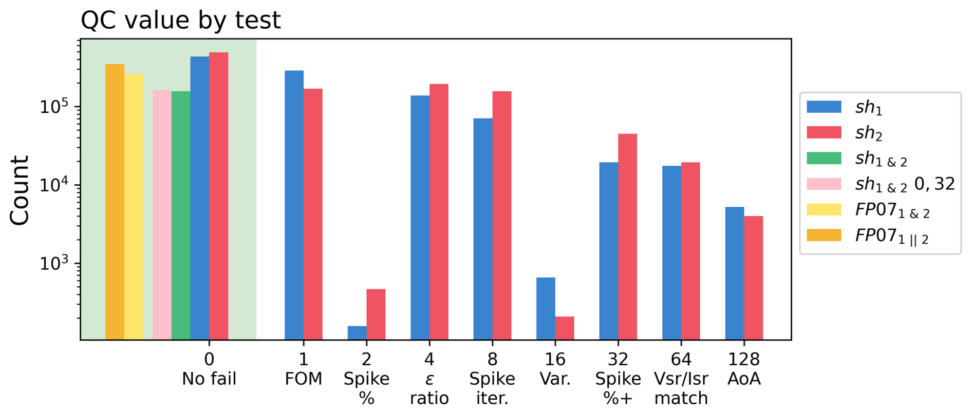
Figure 6 Count of the primary QC flags. Blue and red respectively refer to sh1, sh2 probes. Green indicates the (best) cross-probe choice and pink as a secondary cross-probe choice considering a relaxed despiking fraction criteria. Yellow indicates that both FP07 estimates pass, orange indicates that one of the two passes. Cumulative/combination of flags is not shown.

Table 4 Count of total and QC-passing estimates.

5.4 Distributions of QC-passing estimates by temporal and spatial bins

Figure 7 shows the distribution of valid estimates at both shear probes, with QC = 0 in green and QC = 0 or 32 in pink. Estimates with QC = 0 for both FP07 thermistors are shown in yellow, while values valid for only one thermistor are shown in orange. The yearly counts reflect progressive improvements in deployment and technical reliability, with 2015 and 2017 representing early testing phases. Seasonal coverage is densest from late spring to mid-autumn, although data from late winter and early spring are also included. In terms of spatial distribution, the core of valid estimates is centered around 500 m depth, with a higher density on the eastern side of the section.

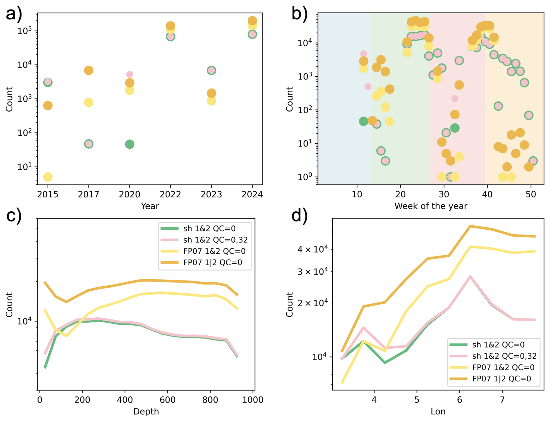
Figure 7 Count of passing data by bins of: years, week of the year, depth, and longitude. Green indicates the (best) cross-probe choice for shears and pink as a secondary cross-probe choice considering a relaxed despiking fraction criteria. Yellow indicates that both FP07 estimates pass; orange one on two.

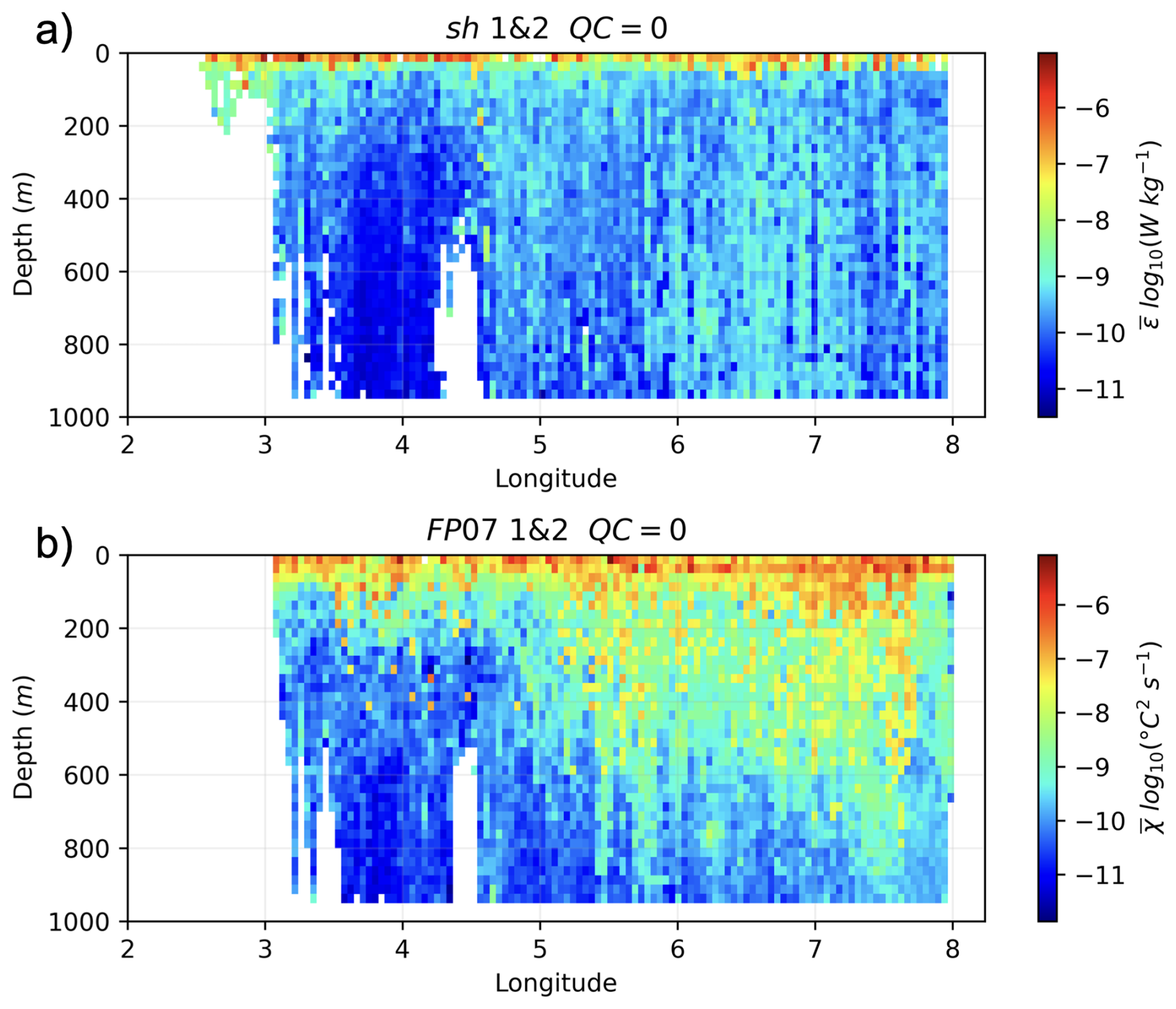
Figure 8 Synthetic sections of all good estimates of ε and χ (all years considered) averaged by depth bins of 25 m, and longitudinal bins of 0.045° (circa 5 km).

5.5 Averages of estimates across the longitudinal section, and their associated distributions

In Fig. 8 we present averaged cross-section of dissipation rate (ε) from shear probes (top) and thermal variance dissipation rate (χ) from FP07 thermistors (bottom), filtered for quality flag QC = 0 (an overview of individual estimates by sensors and years can be consulted in Fig. S2). Both sections highlight the vertical and horizontal distribution of turbulent mixing across the Balearic–Sardinian transect. The ε field reveals distinct near-surface intensification associated with the Atlantic Water (AW) layer, while subsurface peaks are also visible, notably in the Eastern Intermediate Water (EIW) core and near the top of the Western Mediterranean Deep Water (WMDW). Noteworthy enhancements are observed between 4.5 and 5° E in the upper 500 m, and between 6 and 7° E from 500 to 1000 m depth, possibly indicating frontal activity or internal wave breaking. These signals are also evident in χ, which highlights the role of isopycnal exchanges. Around 2.5 to 3.5° E, the transect crosses the diagonal connecting southern Balearic waters to Mallorca, where turbulence appears locally enhanced. A relatively quiescent band between 3.5 and 4.5° E separates this region from the central part of the transect, possibly reflecting a dynamical transition zone.

In Fig. 9 we present the probability density functions (PDFs) of ε and χ after grouping the estimates by layer, longitude, and season. In the vertical decomposition, upper layers show a progressively broader distribution extending toward more intense ε values. The longitudinal breakdown reveals generally similar distributions across the section, with a tendency for higher intensities on the eastern side. Seasonal decomposition shows distinct patterns. Spring and summer exhibit relatively weak dissipation levels, with distributions centered between $\mathit{\epsilon }\approx {\mathrm{10}}^{-\mathrm{11}}$ and 10⁻¹⁰ W kg⁻¹. Autumn shows a bimodal distribution, with a primary mode similar to spring and summer ($\mathit{\epsilon }\approx {\mathrm{10}}^{-\mathrm{11}}$–10⁻¹⁰ W kg⁻¹) and a secondary mode at higher dissipation levels ($\mathit{\epsilon }\approx {\mathrm{10}}^{-\mathrm{9}}$–10⁻⁸ W kg⁻¹). Winter is characterized by substantially higher dissipation rates, typically spanning $\mathit{\epsilon }\approx {\mathrm{10}}^{-\mathrm{8}}$–10⁻⁶ W kg⁻¹, although based on a smaller number of observations. These patterns suggest that autumn captures intermittent energetic events superimposed on a generally weakly dissipative background, while winter conditions favor more frequent and intense turbulence associated with enhanced vertical mixing.

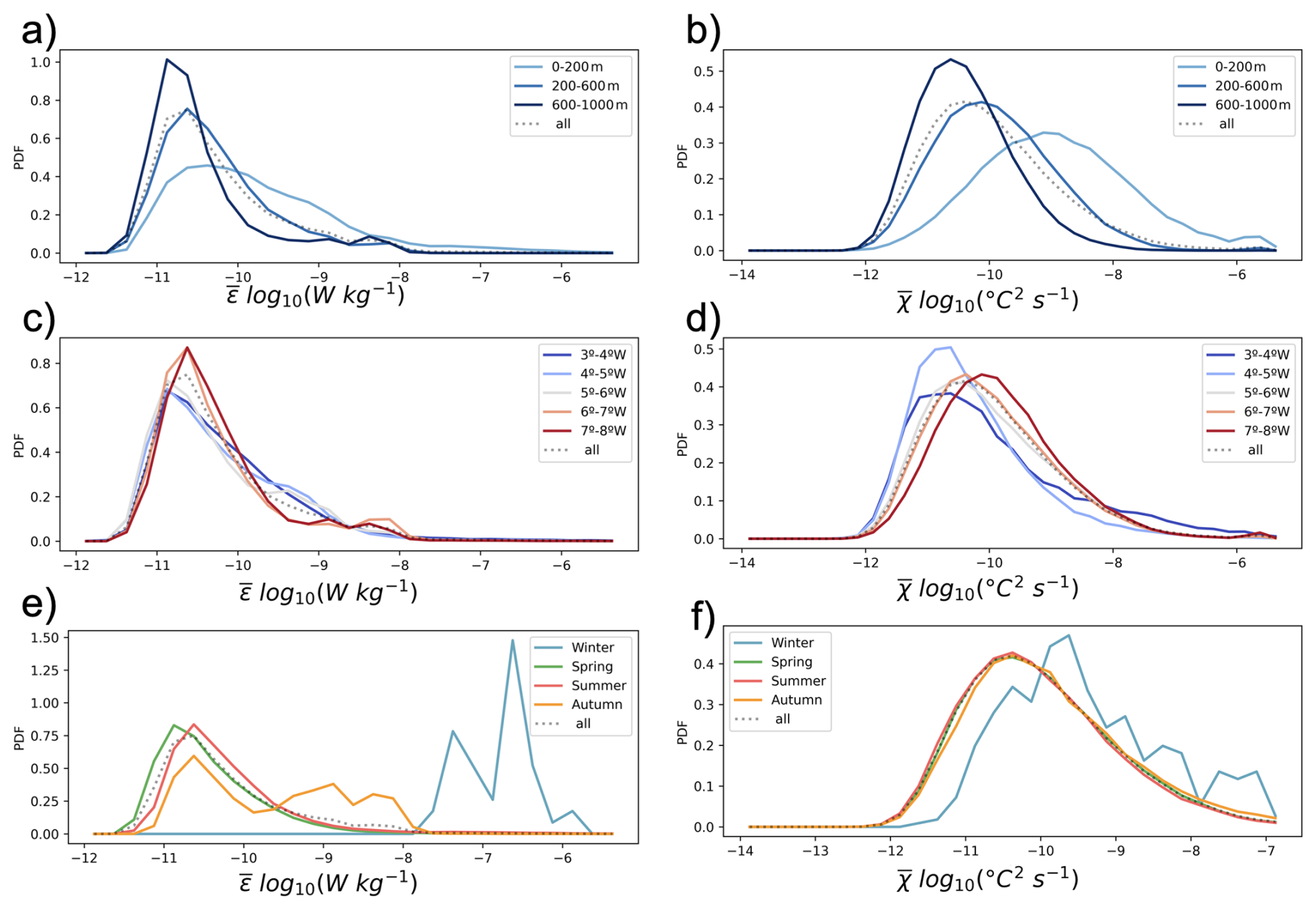
Figure 9 Normalized probability distribution functions (PDF) of cross-checked passing (QC = 0) estimates of ε (a, c, e) and χ (b, d, f) binned by layers, longitudinal fractions and seasons.

For χ, the seasonal contrast is weaker. Spring, summer, and autumn display broadly similar distributions, whereas winter stands out with systematically lower χ values. χ is influenced by both diapycnal mixing and isopycnal stirring, and its seasonal variability likely reflects changes in stratification as well as mesoscale and frontal activity. The reduced χ levels observed in winter are consistent with a weaker stratification and a reduced role of isopycnal stirring, while enhanced χ during the stratified seasons may reflect a combination of small-scale turbulence and lateral stirring processes.

6 Conclusions

Quality control flags discussed here refer to the final L4 QC assigned on a probe-wise basis. The final QC flag is computed as a bitwise combination of all applied quality-control tests. Estimates flagged as QC = 0 correspond to individual shear-probe estimates for which no QC test has failed. This includes spectral fit quality (figure of merit ≤ 1.4), spike contamination, variance resolution, angle-of-attack constraints, and inter-probe ratio and method-consistency checks, noting that these latter tests may reject only one of the two paired estimates. QC = 0 therefore indicates a valid estimate for a given probe, while stricter cross-checked subsets additionally require both probes to simultaneously reach QC = 0. QC = 0 estimates form the core of the L4 product and can be used with high confidence in scientific analyses.

The broader category QC ≤ 1 includes both QC = 0 and QC = 1 estimates. QC = 1 flags estimates for which the figure of merit exceeds 1.4, indicating a poorer fit to the theoretical spectral model (e.g., Nasmyth or Lueck), while other QC criteria remain satisfied. As discussed by Lueck et al. (2024), no universal threshold exists for the figure of merit, as its interpretation depends on platform and environmental conditions.

Flags with QC > 2 indicate failure of one or more critical quality criteria. Common combinations include significant spike contamination (QC = 2 or 8), disagreement between probes (QC = 4), or poor resolution of the turbulent variance (QC = 16). These estimates are not suitable for general use and should either be discarded or considered only after manual inspection and context-specific evaluation.

A special consideration is given to spike-related quality flags, particularly QC = 2 and QC = 32. The QC = 2 flag is assigned when more than 5 % of data points are affected by spikes, despite otherwise valid spectral features and probe agreement. Such spiking may arise from biological interference, local mechanical effects, or valid turbulence partially obscured by benign outliers. In addition, the despiking iteration count flag, QC = 8, is triggered when more than nine despiking passes are needed. However, the literature offers no consensus on acceptable iteration limits (Lueck et al., 2024), and the ODAS routine caps iteration counts at ten, which limits the interpretive strength of this metric. To recover meaningful data in long profiles where spike accumulation may be more likely, we introduce a relaxed quality flag, QC = 32, for cases where the spike fraction falls between 5 % and 15 % and iteration counts remain below the threshold. This intermediate flag acknowledges the potential value of these estimates, especially given that some profiles exceed 1000 m in length. Applying a fixed percentage criterion across records of varying length may unfairly penalize longer profiles, which are more prone to encounter localized spikes. QC = 32 thus represents a compromise: it eventually allows discarded valid data to be included in secondary analyses, without misrepresenting them as core-quality estimates.

In practice, our decision framework recommends using QC = 0 as the primary dataset for scientific interpretation. QC = 32 may be optionally included in context-aware analyses, particularly where spatial or seasonal completeness is important. When examining data from individual probes (e.g., shear1 or shear2 separately), QC = 0 may also be retained under specific conditions, although the absence of cross-validation should be considered. All other QC categories should be excluded from core analyses or subjected to manual review depending on the use case.

This dataset represents one of the most comprehensive glider-based microstructure records collected in the Western Mediterranean to date, spanning nearly a decade from 2015 to 2024. Over this period, deployment protocols and sensor performance progressively improved, resulting in a steady increase in data quality and reliability. The dataset captures multiple seasonal cycles, with denser coverage from late spring through autumn and additional profiles obtained during late winter and early spring. This seasonal breadth allows for the exploration of variability in turbulent mixing under contrasting stratification regimes. By repeatedly surveying a fixed transect between Sardinia and the Balearic Islands, the dataset also provides high-resolution insights into a key hydrographic boundary. This repeated coverage of a dynamic interface aligns with the objectives of the Ocean Gliders Program (Testor et al., 2019), supporting long-term, fine-scale observation of boundary currents, water mass transformation, and vertical mixing in a region of both regional and basin-scale importance.

Despite the strengths of the dataset, several limitations highlight the technical and methodological challenges associated with autonomous turbulence observations. While raw sampling potentially yielded millions of measurement points, strict quality control procedures narrowed the dataset to a validated subset of only tens of thousands of points. This reduction by factors of 100 to 1000 underscores the sensitivity of microstructure measurements to sensor stability, platform dynamics, and environmental conditions. Profiles affected by low incident velocity, strong glider pitch, or localized contamination were routinely excluded. Future improvements could include enhanced real-time monitoring of glider flight and sensor performance, allowing more adaptive sampling strategies. Transmission of diagnostic metadata in near-real time could help identify problematic segments while missions are underway. Additionally, further development of onboard processing and storage, combined with cost-effective and robust sensor solutions, could significantly increase the volume of usable turbulence estimates. The dataset confirms the added value of gliders for observing ocean turbulence, especially when equipped with microstructure payloads such as the Micro Rider. Unlike traditional platforms, gliders deliver continuous, high-resolution vertical sections over hundreds of kilometers without requiring ship support. Their autonomous operation makes them suitable for deployment in remote or challenging environments, offering a sustained observational presence that complements episodic ship-based surveys. Gliders bridge the gap between point measurements from moorings and broad-scale CTD transects and enable four-dimensional views of the ocean when biogeochemical and optical sensors are integrated. Importantly, this dataset demonstrates that key turbulence variables such as ε and χ have reached a level of maturity where they can be regularly retrieved, quality-controlled, and used in scientific and operational contexts. Their inclusion as Essential Ocean Variables is increasingly feasible, with implications for ocean mixing parameterizations, biogeochemical fluxes, and model development (Aydogdu et al., 2025). The approaches documented here can inform broader integration into GOOS, Copernicus, and potentially future Argo extensions, particularly as sensor miniaturization and cost reduction continue to expand the accessibility of turbulence-resolving platforms.

7 Code availability

The MATLAB and Python code used for data processing and quality control is archived on Zenodo at: https://doi.org/10.5281/zenodo.16541936 (Kokoszka, 2025).

A public notebook to read the data and produce the figures can be consulted at https://colab.research.google.com/drive/1qsN8n68C3FBiFkfGt32MGPsthtqM-PmU?usp=sharing (last access: 29 July 2025).

8 Data availability

Turbulence microstructure dataset from Slocum Glider Teresa (Western Mediterranean, 2015–2024) is available from SEANOE at: https://doi.org/10.17882/107995 (Kokoszka et al., 2025). The glider data supporting the microstructure processing are publicly available and correspond to the Sardinia–MAllorca Repeated Transect (SMART) dataset (Chiggiato et al., 2021), hosted by the Balearic Islands Coastal Observing and Forecasting System (SOCIB), https://doi.org/10.25704/ZWMH-AP87.