A six-year circum-Antarctic icebergs dataset (2018–2023)

The distribution of Antarctic icebergs is crucial for understanding their impact on the Southern Ocean's atmosphere and physical environment, as well as their role in global climate change. Recent advancements in iceberg databases, based on remote sensing imagery and altimetry data, have led to products like the BYU/NIC iceberg database, the Altiberg database, and high-resolution SAR-based iceberg distribution data. However, no unified database exists that integrates various iceberg scales and covers the entire Southern Ocean. Our research presents a comprehensive circum-Antarctic iceberg dataset, developed using Sentinel-1 SAR imagery from the Google Earth Engine (GEE) platform, covering the Southern Ocean south of 55° S. A semi-automated classification method that integrated incremental random forest classification with manual correction was applied to extract icebergs larger than 0.04 km², resulting in a dataset for each October from 2018 to 2023. The resulting dataset documents the geographic coordinates and geometric attributes of icebergs (area, perimeter, major axis, and minor axis), provides uncertainty estimates for area, and, under a fixed density assumption, employs the Iceberg Size Scaling to derive iceberg mass along with the associated uncertainty bounds. The dataset reveals significant interannual variability in iceberg number and total area. Specifically, the number of icebergs increased from 34 825 in 2018 to approximately 51 420 in 2021, while the total area expanded from 38 668 to 52 276 km², both corresponding to major ice shelf calving events, followed by a decline in 2022. The annual average total iceberg area is 44 859 ± 4900 km², and the average mass is 9162 ± 1935 Gt. Validation using test set samples shows that the integrated incremental random forest classification achieves accuracy, recall, and F1-score exceeding 0.90. Comparisons with existing iceberg products (including the BYU/NIC iceberg database and the Altiberg database) indicate a high consistency in spatial distribution, while our dataset demonstrates clear advantages in terms of spatial coverage, iceberg detection scale, and identification capabilities in regions with dense sea ice. This dataset serves as a novel data resource for investigating the impact of Antarctic icebergs on the Southern Ocean, the mass balance of ice sheets, the mechanisms underlying ice shelf collapse, and the response mechanisms of iceberg disintegration to climate change. The iceberg dataset is publicly available at https://doi.org/10.5281/zenodo.17165466 (Liu and Chen, 2025).

1 Introduction

Icebergs are large freshwater ice masses that break off from the edges of ice sheets, ice shelves, or glaciers and enter the ocean. They are a critical component in the global climate system (Benn and Åström, 2018). Approximately half of the mass loss from the Antarctic ice sheet is discharged into the Southern Ocean through iceberg calving (Depoorter et al., 2013; Rignot et al., 2013; Liu et al., 2015). Annually, the dissolution of over 100 000 icebergs into the ocean is estimated to introduce a volume of freshwater that, according to certain calculations, exceeds the global annual freshwater consumption (Qadir et al., 2022; Orheim et al., 2023). This resultant freshwater influx plays a critical role in influencing the thermohaline characteristics, heat content, and freshwater balance within the impacted regions of the Southern Ocean (Gladstone et al., 2001; Hammond and Jones, 2016). On the bottom, grounding icebergs can interact with ocean floor and leave scours as a kind of geological record (Dowdeswell and Bamber, 2007; Li et al., 2018; Liu et al., 2021). Additionally, the nutrients carried by icebergs can influence the spatial distribution of primary productivity (Duprat et al., 2016), promoting the development of local ecosystems (Smith et al., 2007; Wu and Hou, 2017; Lin et al., 2024). Furthermore, icebergs pose a potential threat to maritime activities (Bigg et al., 2018), as human activity in the Antarctic region increases, accurate monitoring of iceberg distribution, size, and trajectory prediction has become critical (Evans et al., 2023)

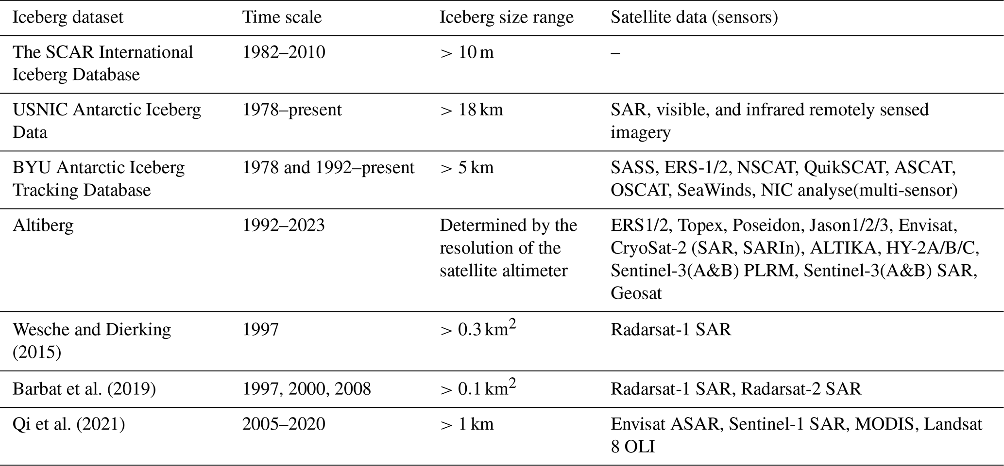
The current databases on the distribution of Antarctic icebergs, as shown in Table 1, are primarily categorized into four types: (1) Ship-based observations, such as the SCAR International Iceberg Database (Orheim et al., 2023), compiled and published by the Norwegian Polar Institute (NPI) and the Scientific Committee on Antarctic Research (SCAR), which records 323 520 icebergs and serves as an important historical dataset. However, it is only confined to shipping lanes, not fully representing the Antarctic iceberg's spatial distribution and its interannual changes; (2) Low-resolution satellite imagery-based databases, with the U.S. National Ice Center (USNIC) and Brigham Young University (BYU) Antarctic Iceberg Database as a notable example (Long et al., 2002; Stuart and Long, 2011a, b). Budge and Long (2018) consolidated these databases to offer iceberg location, length, and area data, but they are restricted to larger icebergs (length>5 km) due to the limitations of low-resolution imagery; (3) Satellite radar altimetry-based databases, like the Altiberg database from the French Research Institute for Exploitation of the Sea (Tournadre et al., 2012, 2015, 2016). This database is effective at detecting icebergs in open waters, but in complex scene, such as areas with dense ice or high iceberg concentrations, it becomes challenging to extract accurate iceberg information from the altimetric waveforms; (4) High-resolution SAR data-derived products. Wesche and Dierking (2015) extracted icebergs larger than 0.3 km² in the Antarctic coastal region using Radarsat-1 circum-Antarctic mosaic images. Barbat applied a random forest algorithm to Radarsat circum-Antarctic mosaic images from 1997, 2000, and 2008 to obtain iceberg distributions for the corresponding years (Barbat et al., 2019a); (5) circum-Antarctic iceberg calving dataset. This dataset was derived from continuous optical (MODIS and Landsat-8) and radar (Envisat ASAR and Sentinel-1) satellite observations and was released by Qi et al. (2021). The product provides detailed information on each calving event, including time, area, size, thickness, etc., but it only focused on the transient icebergs just calved from ice shelves therefore lacking the spatial distribution across the open ocean. All above data products primarily cover the Antarctic coastal region, and the published datasets are not real-time monitoring results, but rather used for historical scientific research. In summary, there is currently no comprehensive iceberg database covering multiple scales and the entire Southern Ocean has been established to date.

Table 1 Overview of Antarctic Iceberg Datasets.

High-precision, large-scale, and long-term continuous remote sensing observations of circum-Antarctic iceberg distribution not only characterize the spatiotemporal patterns of iceberg occurrence but also provide critical data for elucidating the mechanisms of iceberg formation and evolution, ice-shelf dynamics, and their complex interactions with climate change. In this study, we leveraged the Google Earth Engine (GEE) platform to acquire Sentinel-1 SAR mosaic imagery and applied an incremental random forest classification combined with manual correction to identify Antarctic icebergs larger than 0.04 km², extracting each iceberg's outline, location, area, mass, and associated uncertainty. Based on these results, we constructed a circum-Antarctic iceberg distribution dataset covering each October from 2018 to 2023 and conducted a comprehensive analysis of the spatiotemporal characteristics of iceberg distribution over this six-year period. To ensure the reliability of the dataset, we performed an internal accuracy validation of the classifier and conducted external validation by comparing our results with existing iceberg databases and data products.

2 Data

To identify circum-Antarctic icebergs, we utilized the European Space Agency (ESA) Sentinel-1 C-band SAR Ground Range Detected (GRD) data. Given the extensive coverage of the data, we chose the Extra Wide (EW) swath mode, which provides a spatial resolution of 40 m. The Sentinel-1 data offers various band combinations based on different polarization modes (e.g., VV, HH, VV + VH, and HH + HV), with HH polarization being the primary mode available in polar regions (Koo et al., 2023; Ferdous et al., 2018). Therefore, only HH polarization band images were used for analysis.

To optimize iceberg detection, HH-polarized backscatter time series were extracted from representative fixed pixels for icebergs, first-year ice, multiyear ice and open water in Sentinel-1 GRD imagery, sampled every five days from January 2018 to December 2021. The iceberg pixel remained grounded throughout the study, yielding approximately 60 observations per year (≈5 per month), with comparable sampling frequencies for the other typical Antarctic oceanic features. Each pixel's time series was then resampled on a monthly basis to compute mean backscatter coefficients and variances, and the resulting mean curves with shaded standard-deviation uncertainty are shown in Fig. 1. As noted by Drinkwater et al. (1995) in their study of sea ice in the Weddell Sea, distinct differences in backscatter coefficients exist between various oceanic features. For instance, rough and undisturbed first-year ice, second-year ice, and other ice types exhibit unique reflective properties, which become more pronounced with seasonal and environmental changes. Environmental factors such as temperature and heat flux cause significant variation in backscatter coefficients. By comparing the interannual backscatter coefficient trends of typical Antarctic oceanic features, it was found that from June to October, the backscatter coefficient of icebergs is significantly higher than that of fast ice, first-year ice, and open water (Wesche and Dierking, 2012, 2015; Mazur et al., 2017), especially in October when the backscatter coefficient of fast ice reaches its annual minimum, providing optimal conditions for distinguishing icebergs from other oceanic features. Based on the above analysis, we selected Sentinel-1 SAR data in October for each year.

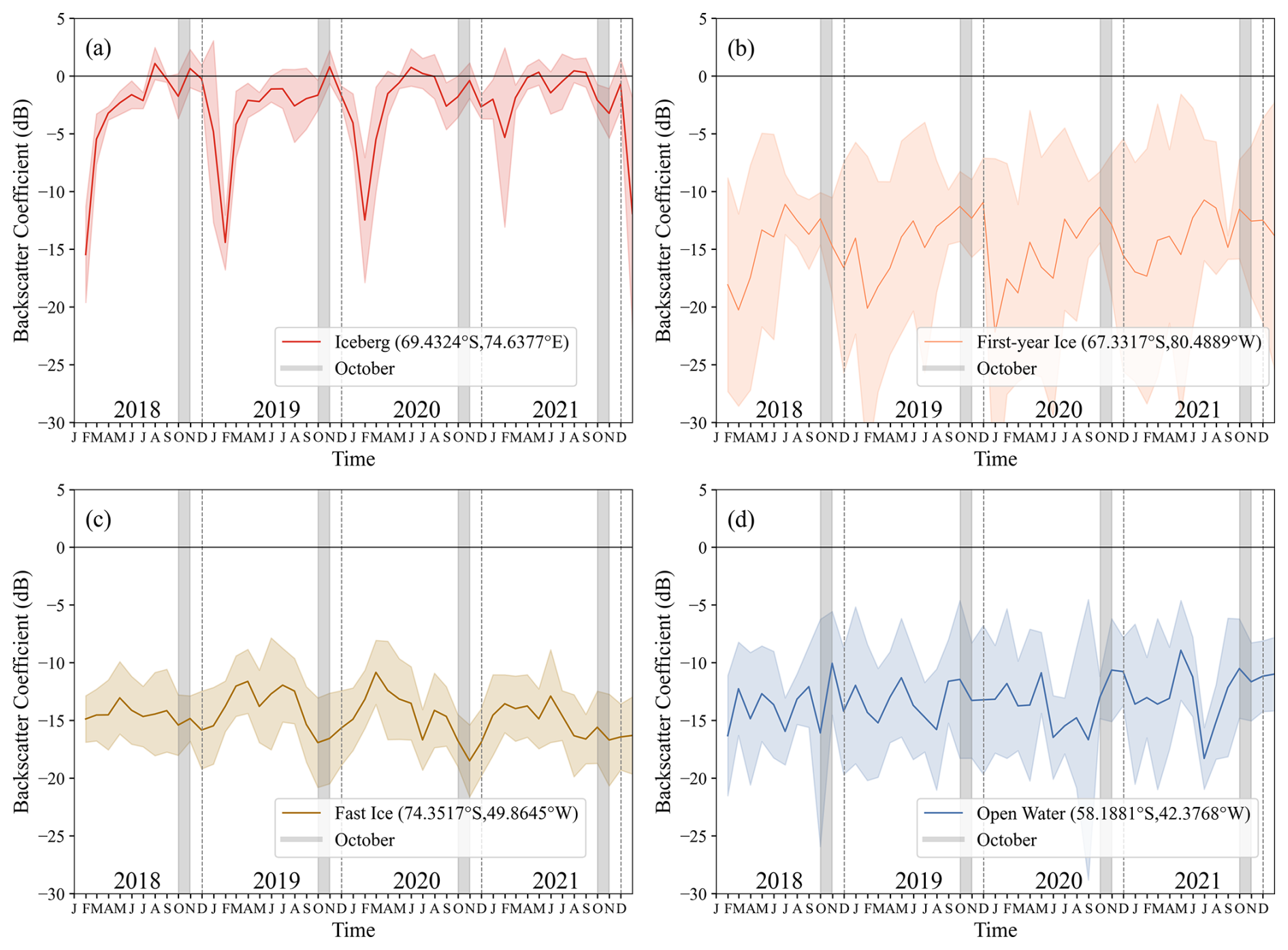
Figure 1 Time series of backscatter coefficients for typical Antarctic surfaces from 2018 to 2021: (a) iceberg, (b) first-year ice, (c) fast ice, and (d) open water. Each time series corresponds to a single pixel. The solid colored lines represent the monthly average backscatter coefficients derived from the 5 d sampling intervals, while the shaded regions indicate the uncertainty intervals corresponding to one standard deviation. Gray-highlighted areas indicate the selected months (October of each year).

3 Method

The semi-automated workflow for extracting Antarctic icebergs using machine learning is shown in Fig. 2 and consists of four subprocesses: (1) Data acquisition, (2) Image segmentation, (3) Iceberg detection, and (4) Iceberg attribute extraction. In this section, we will provide the technical methods and details for each subprocess.

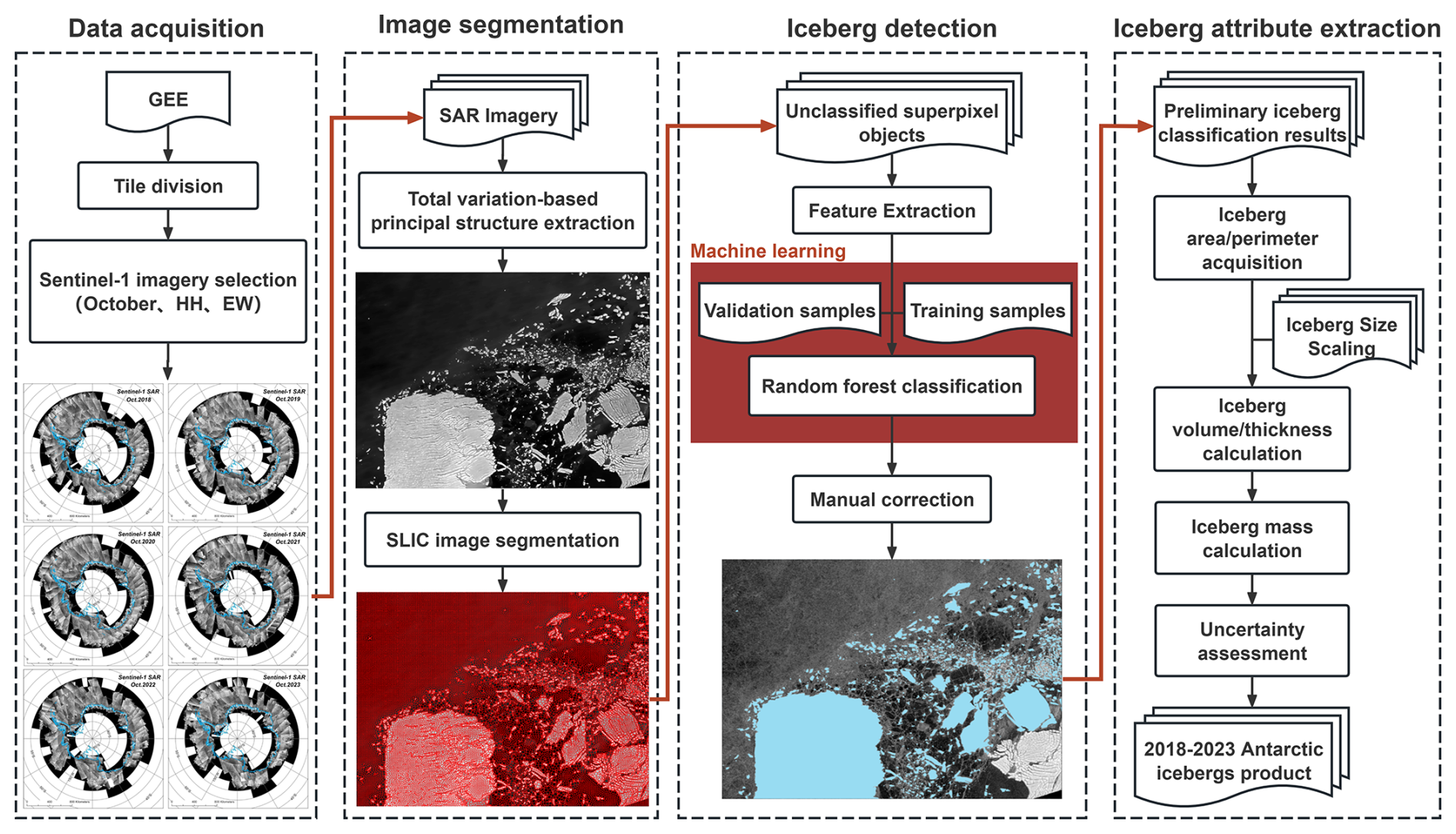
Figure 2 Flowchart of our methodology to obtain the 2018–2023 Antarctic iceberg product.

3.1 Data acquisition

GEE is a cloud-based platform developed by Google for the visualization and analysis of geospatial data. Through GEE, users can easily access a wide area of satellite remote sensing datasets (Gorelick et al., 2017; Amani et al., 2020). The Sentinel-1 SAR data provided by GEE have been pre-processed to remove thermal noise, apply radiometric calibration, and perform terrain correction, resulting in GRD backscatter coefficient images (expressed in dB). Given the vast extent of the Southern Ocean, this study divides the region south of 55° S into 5°×5° tiles, resulting in a total of 360 tiles annually. For each tile, we retrieved Sentinel-1 SAR HH-polarization data from the EW swath mode acquired in October of each year between 2018 and 2023 (Fig. 3), and mosaicked the data chronologically to create monthly composite images, with later-acquired images overwriting valid pixels in earlier ones to fill voids at the beginning of the month. Statistics show that most tiles contain 2–4 images from different dates: in each year, more than 50 % of tiles have a maximum date span of ≤5 d, and more than 90 % have a maximum span of ≤10 d (Fig. S1 in the Supplement). In addition, we delineated the effective observation area for each year and determined the intersection and union of these areas across the different years. The intersection of the effective observation ranges over six years has reached 16.67×10⁶ km², nearly covering the sea regions where icebergs might exist, thereby providing data support for obtaining the distribution of circum-Antarctic icebergs. In the subsequent analysis of annual variation, we primarily focused on comparing icebergs within the intersecting observation areas across years, in order to identify trends in iceberg numbers and distribution. We emphasized this comparison in the consistent dimension, ensuring that the trends we observed were on an equal footing and thus more reliably indicative of actual changes in the iceberg population. Furthermore, to quantitatively assess the issues of misclassification, omission, iceberg merging, and contour deviations in the iceberg dataset, we selected four 5°×5° tile sample areas with low ocean current speeds and slow iceberg drift (as indicated by the yellow regions in Fig. 3). These sample areas effectively reflect the uncertainties in iceberg detection under complex ocean conditions and thus serve as representative of the overall detection performance of the entire dataset.

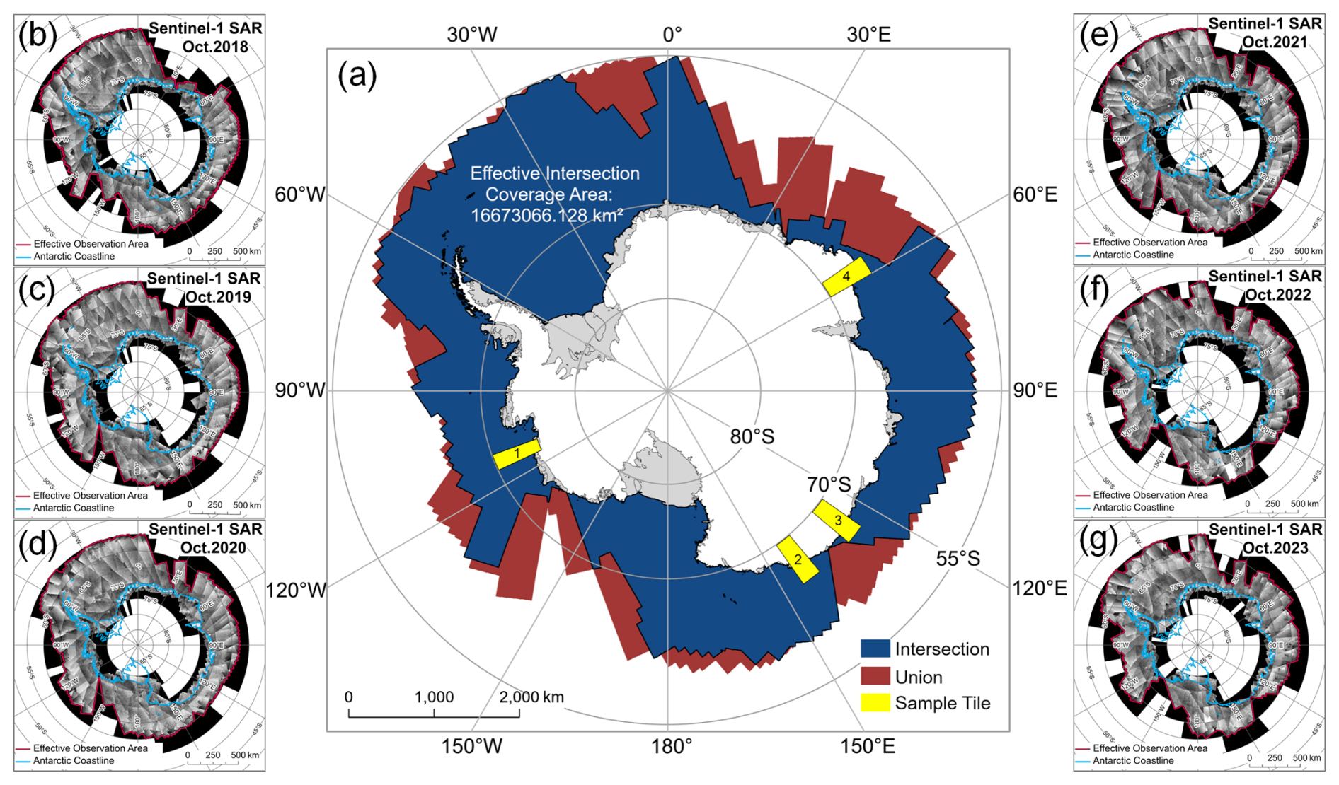
Figure 3 Circum-Antarctic Sentinel-1 SAR Data. The left and right columns display the Sentinel-1 mosaic images acquired from 2018 to 2023 on the GEE platform. The blue line delineates the coastline, while the red line indicates the valid observation boundaries. The central map illustrates the intersection and union of the observation areas over the six-year period, along with the four selected 5°×5° tile sample areas.

3.2 Image segmentation

3.2.1 Total Variation-based principal structure extraction (TV) algorithm for Sentinel-1 images smoothing

Due to the presence of background features such as sea ice and sea water, the edges and shapes of icebergs in SAR images can be unclear. To address this issue, we applied a Total Variation-based principal structure extraction (TV) algorithm (Xu et al., 2012), which separates the SAR images into two layers: a background texture layer and a primary structure layer that represents the shape characteristics of the ocean surface. By extracting the primary structure layer, we were able to enhance the visibility of the iceberg edges and improve the accuracy of contour detection. The TV algorithm is particularly effective when the size of the background textures differs substantially from that of the primary structures, as it preserves the image edges and clarifies the boundaries. The results (Fig. 4) show that the TV algorithm successfully reduced background interference, retaining only the main contours of the icebergs, which made the iceberg bodies and boundaries much distinct. Even in complicated scene (Fig. 4c) or for small icebergs only a few hundred meters in size (Fig. 4b), the algorithm was able to effectively extract their contours.

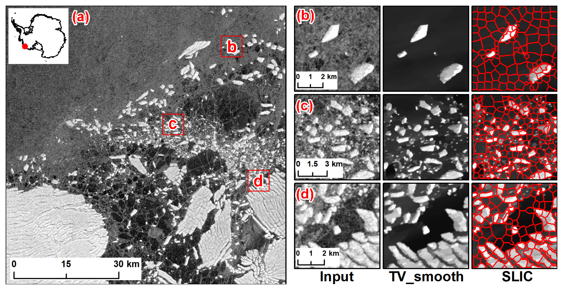
Figure 4 The results of the TV algorithm and SLIC segmentation on SAR imagery are shown in the following panels. Panel (a) provides an overview of the study area, with three representative sub-regions highlighted. Panels (b)–(d) show enlarged views of these sub-regions, presenting the original SAR image, the denoised output from the TV-smoothing algorithm, and the segmented image generated by the SLIC algorithm, respectively.

3.2.2 Simple Linear Iterative Clustering (SLIC) image segmentation

We applied the Simple Linear Iterative Clustering (SLIC) algorithm for superpixel segmentation on the smoothed SAR images to avoid noise amplification and reduce computational complexity that may arise from using individual pixels during the subsequent Random Forest (RF) classification (Mazur et al., 2017; Karvonen et al., 2022; Koo et al., 2023). A superpixel is defined as a small, contiguous cluster of adjacent pixels that share similar backscatter characteristics, effectively representing a meaningful image region rather than individual pixels. By grouping pixels with similar backscatter characteristics into small, connected clusters, referred to as “superpixels”, we not only improved classification efficiency but also significantly decreased the computational burden during the classification process (Achanta et al., 2012). The results of superpixel segmentation on the SAR images used in this study are shown in Fig. 4, with superpixel outlines displayed independently and not combined. Compared to the original image, the SLIC algorithm effectively delineates the boundaries of oceanic features and adapts well to different categories.

Given the large volume of image data and the spatial variability of iceberg distribution, we adopted a two-stage segmentation approach. In the first stage, we performed coarse segmentation using larger superpixels (40×40 pixels). For superpixels exhibiting histograms with multiple peaks, we then applied finer segmentation using smaller superpixels (5×5 pixels). This approach ensures that the smallest detectable iceberg has a length greater than 200 m or an area larger than 0.04 km².

3.3 Iceberg detection

3.3.1 Feature extraction

After image segmentation, we extracted features for each superpixel object based on the segmentation labels applied to the original, unprocessed image. These features were then used to construct a feature set for classification. In conjunction with manual interpretation, a sample set was created for the subsequent classification process. The extracted object features were categorized into three types: Statistical features, histogram-based features, and texture features, resulting in a total of 24 features. A detailed description and explanation of these features can be found in Appendix A.

3.3.2 Incremental random forest classification

In this study, we employed an ensemble incremental random forest (RF) classifier (Zhou, 2012) to identify Antarctic circumpolar icebergs. The process consisted of two main steps: (1) Using the training and validation sample sets, we evaluated the classification performance of various feature combinations, optimized the parameters of each RF classifier, determined their weights and classification thresholds, and constructed the ensemble classifier; (2) For each tile, we performed incremental RF training and classification on the superpixel objects, enabling automated iceberg detection.

Construction of Incremental random forest classifiers

Based on the Sentinel-1 SAR imagery, we applied the SLIC algorithm to generate superpixels and then manually selected approximately 2000 superpixel samples per year, evenly split between icebergs and non-icebergs. The sample set was then randomly divided into three subsets: an initial training set, a validation set, and a test set, in a $\mathrm{6}:\mathrm{2}:\mathrm{2}$ ratio. The training set was used to train the RF classifier, the validation set to tune parameters and the test set to assess generalization performance.

Taking October 2018 as an example, we detailed how we determined the parameters for our ensemble of random forest classifiers and performed an incremental training procedure within each 5°×5° tile. We constructed four independent random forest models: RF1 trained on statistical features, RF2 on histogram features, RF3 on texture features, and RF4 on all combined features. Classifier settings were determined from out-of-bag (OOB) error curves, with stable minima selected as optimal: 200 trees/3 features for RF1, 100 trees/5 features for RF2, 250 trees/7 features for RF3, and 150 trees/3 features for RF4 (Fig. S2 in the Supplement). Each independent random forest model was then evaluated on the validation set to compute accuracy, precision, recall, and F1 score. Using each metric in turn for normalization, we generated four candidate weighting schemes, thereby avoiding reliance on a single evaluation criterion.

For the ensemble in 2018, we multiplied each model's iceberg probability by its corresponding weight and summed the results to obtain a combined discriminant score for each superpixel. We tested decision thresholds from 0 to 1 (step 0.01) on the validation set, plotting Precision-Recall (P-R) and Receiver Operating Characteristic (ROC) curves (Fig. S3 in the Supplement). The scheme that maximized the combine areas under the P-R curve and ROC curve was selected as optimal, as this balances precision-recall trade-offs with overall classification performance. This yielded weights of 0.218, 0.271, 0.246 and 0.265 for RF1–RF4, respectively. Finally, we determined the threshold that maximized the F1 score on the validation set, and set 0.783 as the final decision threshold for iceberg detection. The same procedure was applied to the remaining years to obtain optimal parameter configurations for each year, with the specific settings presented in Table S1 in the Supplement.

Automated Antarctic iceberg identification

After constructing the ensemble RF classifier, we predicted all the superpixels within each 5°×5° tile. Given the complexity of the data within each tile, image segmentation typically produces tens of thousands to hundreds of thousands of superpixels that require classification. Given the limited size of the initial training sample and the potential variation in iceberg and non-iceberg characteristics across different tiles, we adopted an incremental random forest approach for each tile. This method uses Mahalanobis distance to allow the classifier to adaptively learn and better match local data characteristics.

The process began by training RF1–RF4 using the initial training set, which were then combined into an ensemble classifier to generate the initial classification results for the tile. Then, we randomly selected an equal number of iceberg and non-iceberg samples from the newly identified objects to expand the training set. Based on feature importance ranking (Fig. S2), we selected the most significant three features to construct the feature space for icebergs and non-icebergs. Subsequently, we calculated the mean (μ) and standard deviation (σ) of the distances between iceberg samples and the center of the iceberg, as well as the mean distance from non-iceberg samples to the iceberg center. If the mean distance from non-iceberg samples to the iceberg center exceeds μ+σ, or the iteration count did not exceed five, we retrained the classifier with the incremental samples. The iteration limit of five was determined through multiple experiments. The incremental learning process terminates when either the conditions were not met or the iteration limit was reached. The predicted iceberg results from the final iteration were then taken as the final classification results for that tile.

For the final classification, all superpixels identified as icebergs were converted into a binary mask, which was then subjected to hole filling and noise removal. We then applied a connected-component labeling algorithm to automatically aggregate all contiguous iceberg superpixels into individual iceberg objects. Two iceberg entities were recognized as distinct only if they were separated by at least one non-iceberg superpixel.

3.3.3 Manual correction

The automatically classified superpixels labels identifying icebergs were used to generate iceberg outlines based on the geographic coordinates of the SAR images. These outline vectors were then manually refined in ArcMap 10.8 software interactively to ensure they accurately represent the true shapes of the icebergs as observed in the corresponding SAR image. Manual correction addressed three main issues: (1) the automatic detection process still resulted in misclassifications and missed icebergs; (2) some iceberg contours were incomplete at the tile boundaries; and (3) due to the mosaic nature of the tiles, some fast-moving icebergs with distinct shape and texture features were segmented into multiple fragments. The results for the four sample areas after incremental random forest classification and manual correction are shown in Fig. 5.

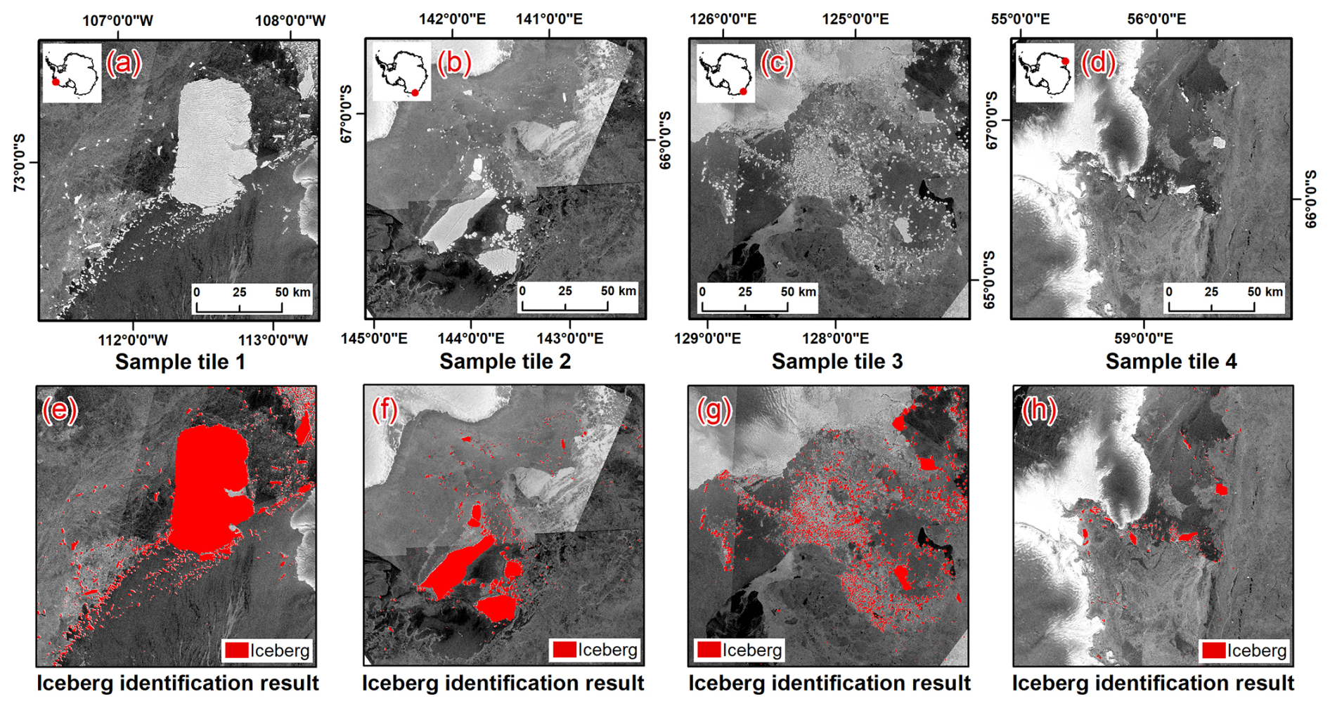
Figure 5 Iceberg identification results, panels (a)–(d) display the Sentinel-1 SAR images from the sample areas, while panels (e)–(h) present the classification results derived from these images using an incremental random forest classification supplemented with manual corrections. In these panels, the red vectors denote icebergs.

3.4 Iceberg attribute extraction

For each iceberg, key attributes such as area, perimeter, long axis, short axis, average thickness, mass, and the associated uncertainties for these parameters were calculated. This section outlines the methods used to derive these iceberg attributes and assess the uncertainties involved.

After obtaining the iceberg outline vector data, we calculated the area (km²) and perimeter (km) of each iceberg under the Antarctic Polar Stereographic projection (EPSG:3031). Based on the area data, we applied the Iceberg Size Scaling to estimate both the mass of individual icebergs and the annual total iceberg mass across the circum-Antarctic region (Gladstone et al., 2001; Stern et al., 2016). Specifically, we used the 10-class iceberg classification scheme from Stern et al. (2016), which provides standardized iceberg properties (mass, length, area, and thickness) spanning from small fragments to kilometer-scale icebergs for use in ocean general circulation models. For each class, we converted the prescribed mass to volume using an iceberg density of 850 kg m⁻³, generating 10 discrete area-volume pairs. A power-law relationship was then fitted to these data points to derive the volume estimation formula for small icebergs (Eq. 1). Based on Eq. (1), the physical thickness limit of 250 m defined by Stern et al. (2016) corresponds to a critical area of approximately 0.67 km². For icebergs smaller than this threshold, volume is calculated directly from the power-law relationship, whereas for larger icebergs, volume is derived by multiplying the area by the fixed thickness of 250 m. Assuming an average density of 850 kg m⁻³, the mass of each iceberg and the circumpolar total are then obtained accordingly in Eq. (2).

$$\begin{array}{}\text{(1)}& {\displaystyle }{V}_{\text{Iceberg}}=\mathrm{7.64}{A}^{\mathrm{1.26}}\text{(2)}& {\displaystyle }M=A_{\text{Iceberg}}\times H\times {\mathit{\rho }}_{\text{Iceberg}}=V_{\text{Iceberg}}\times {\mathit{\rho }}_{\text{Iceberg}}\end{array}$$

Due to the diverse shapes of icebergs, we used the principal orientation method to determine their geometric characteristics. First, we calculated the centroid of the iceberg's geometry, which serves as its geometric center. Then, we applied Principal Component Analysis (PCA) to the iceberg's boundary points to determine the directions of its principal axes. The first principal component corresponds to the long axis of the iceberg, while the second principal component corresponds to the short axis. Next, we projected the boundary points along the long axis and computed the projection length in this direction to obtain the length of the iceberg's long axis, and we used the same method to obtain the length of the short axis.

3.5 Uncertainty assessment

3.5.1 Iceberg area uncertainty

The uncertainty in iceberg area measurement primarily arises from three independent factors: (1) the spatial resolution limitations of SAR imagery; (2) the detection errors introduced during iceberg identification (e.g., misclassification, omission, or merging of iceberg targets); and (3) duplication errors in iceberg counts arising from the image mosaicking process.

The uncertainty due to image resolution (U₁) can be approximated as the product of the total iceberg perimeter and the pixel size of the imagery, that is, we estimate the area uncertainty from the pixel error along the iceberg boundaries using Eq. (3):

$$\begin{array}{}\text{(3)}& U_{\mathrm{1}}=P\times \mathrm{\Delta }x\end{array}$$

Where P is the total perimeter of all icebergs each year (km), and Δx is the spatial resolution of the imagery, which is 40 m.

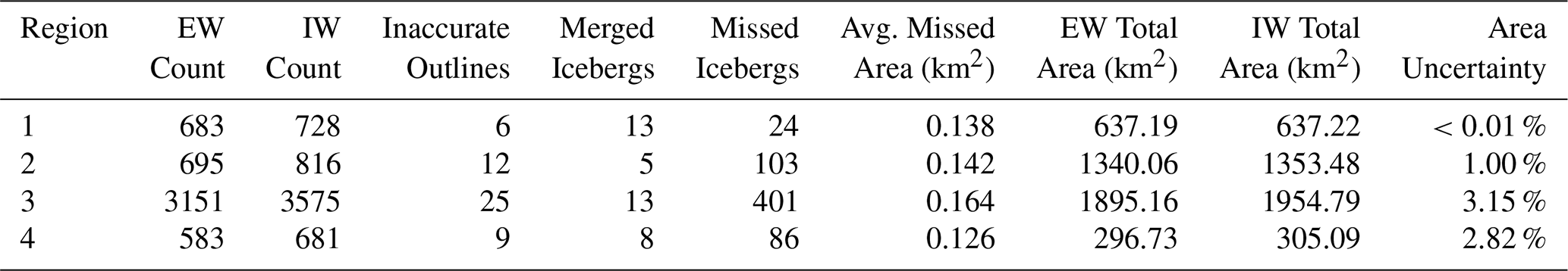
The second source of uncertainty (U₂) primarily arises from errors in iceberg classification and extraction, such as omissions, false detections, erroneous merging (i.e., mistakenly detecting adjacent icebergs as a single object), and contour deviations. To quantitatively evaluate this component, we acquired mosaic images in the Interferometric Wide (IW) swath mode (with a spatial resolution of 20 m) from four 5°×5° sample tile areas, while ensuring that, in iceberg-dense areas, the time interval between the IW mode images and the EW mode images (with a spatial resolution of 40 m) did not exceed 10 d. In each sample tile area, we manually digitized iceberg outlines from high-resolution IW images to construct a reference dataset representing the “true” iceberg count and area, and then compared it with the dataset obtained from EW mode imagery using an incremental random forest algorithm supplemented with manual corrections. As shown in Table 2, the comparison results indicate that in the most complex sample area, the relative error in total iceberg area reached up to 3.15 %. For a conservative estimation of uncertainty, we adopt 4 % as the parameter – i.e., the uncertainty due to detection errors is calculated by multiplying the annual total iceberg area by 4 %.

Table 2 Validation of iceberg detection in four sample regions. Iceberg counts from EW and IW imagery, detection errors (inaccurate outlines, merged and missed icebergs), average missed iceberg area, total iceberg areas, and relative area uncertainty (%) are presented.

The third source of uncertainty (U₃) arises from duplicate counting during image mosaicking,when the same iceberg is recorded in adjacent scenes. Despite manual corrections, small icebergs lacking distinctive shape or texture features cannot always be matched reliably. To quantify this effect, we used the 2021 Antarctic mosaic via GEE, extracting acquisition dates (YYYYMMDD) for each pixel (Fig. S4 in the Supplement). For every iceberg smaller than 10 km², we assigned the centroid pixel's date and computed the distance to the nearest pixel acquired later in time. If this distance was less than the product of the date difference and the mean drift speed, the iceberg was flagged as a potential duplicate. Previous regional studies report mean drift speeds of about 3–7 km d⁻¹ (Hamley and Budd, 1986; Collares et al., 2018; Barbat et al., 2021; Orheim et al., 2023), and we adopted 5 km d⁻¹ as a representative value. In 2021, 1757 icebergs were identified as potential duplicates, representing 3.36 % of the total count and 1.25 % (655 km²) of the total iceberg area. We therefore assign 2 % as the uncertainty contribution from duplicate counting, representing a conservative cross-year upper limit.

The uncertainty in the total annual iceberg area (U_A) can be calculated using the error propagation law, as shown in Eq. (4):

$$\begin{array}{}\text{(4)}& U_{\mathrm{A}}=\sqrt{U_{\mathrm{1}}^{\mathrm{2}}+U_{\mathrm{2}}^{\mathrm{2}}+U_{\mathrm{3}}^{\mathrm{2}}}.\end{array}$$

It should be noted that for an individual iceberg, its area uncertainty is solely determined by the image resolution (U₁), since an iceberg is either correctly extracted or not detected at all; whereas for the total annual iceberg area, both U₁, U₂ and U₃ must be considered, and the overall error is calculated using Eq. (4).

3.5.2 Iceberg mass uncertainty

We employed a two-segment area–volume parameterization combined with a nonparametric bootstrap approach to assess uncertainties in iceberg mass. For small icebergs with an area less than 0.67 km², volumes were estimated using a power-law regression in logarithmic space ($\ln V=b_{\mathrm{0}}+b_{\mathrm{1}}\ln A$), calibrated against the area-thickness parameterization scheme provided by Stern et al. (2016). By repeatedly resampling this calibration dataset, we obtained empirical distributions of the regression parameters (b₀, b₁) and propagated them to derive confidence intervals for total mass. For large icebergs with an area greater than 0.67 km², a fixed thickness of 250 m was assumed. To account for uncertainty in this assumption, the equivalent thickness distribution inferred from the power-law fit at the threshold area was used as a proxy and extrapolated to all large icebergs to construct mass intervals. Finally, we report point estimates and 95 % confidence intervals for the mass of individual icebergs as well as the total Antarctic iceberg mass, with mass uncertainty for small icebergs mainly arising from regression fitting and those for large icebergs primarily arising from the fixed-thickness assumption.

4 Validation and uncertainty

4.1 Accuracy assessment of Antarctic iceberg identification algorithm

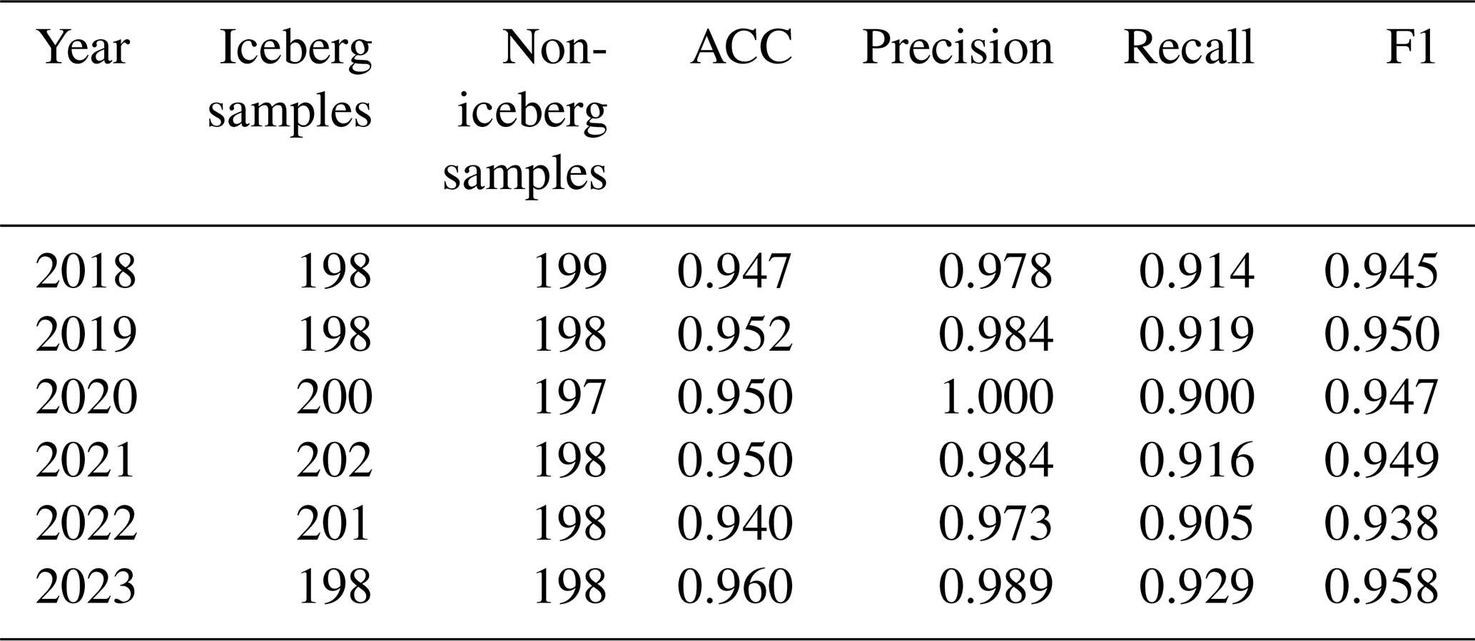
Using approximately 400 manually labeled superpixel samples per year as independent test sets, we conducted year-by-year accuracy assessments of the incremental ensemble random forest classifier for the corresponding years. The evaluation results demonstrate that the classifier consistently maintained high performance in circum-Antarctic iceberg detection throughout the 2018–2023 (Table 3). All performance metrics, including accuracy, precision, recall, and F1-score, exceeded 0.90, indicating that the model possesses robust and reliable classification capability. Furthermore, the inter-annual variation in both classifier weights and discrimination thresholds remained minimal (Table S1), providing evidence that the trained model exhibits good stability under different environmental conditions.

Table 3 Performance evaluation of the incremental random forest classifier.

After classifier performance evaluation, our data product incorporates a manual correction step in addition to the machine learning-based automated iceberg detection (see Sect. 3.3.3). By visual inspection and manually correcting the automated classification results, we further reduced instances of false positives and false negatives. As a result, the final iceberg data product demonstrates even higher precision across various accuracy metrics.

4.2 Attribute uncertainties of Icebergs

Based on a comparison of the results from four sample areas (Table 2), we found that iceberg omissions are relatively severe, resulting in an underestimation of the total iceberg amount by approximately 3 %–15 %. However, the missed icebergs are mainly small or weak-signal targets, with an average area of only 0.126–0.164 km², thus having a limited impact on the total iceberg area. In low-resolution imagery, the radar signal of small icebergs is often weak or their boundaries become blurred due to noise and complex sea conditions, making it challenging to accurately identify all icebergs even after manual correction. Furthermore, in the SLIC algorithm, the low contrast between icebergs and sea ice or open water in low-resolution images leads to blurred iceberg edges, making the boundaries between adjacent icebergs indistinct and causing nearby icebergs to be erroneously merged into a single object or to exhibit contour deviations. Given that false detections are negligible after manual correction, the maximum area uncertainty due to iceberg detection errors in the tile sample areas is 3.15 %. Therefore, we adopt 4 % as a conservative and reasonable estimate.

In addition to omission and classification errors, duplicate counting can also introduce errors in both iceberg number and area estimates. Such issues mainly occur in swath or mosaic overlap regions, where even after manual correction, small icebergs lacking distinctive shape or texture features may still be recorded multiple times, leading to an overestimation of local counts. For example, in 2021 the potential duplicate icebergs had an average area of 0.37 km², accounting for 3.36 % of the total number, whereas they represented only 1.25 % of the total area. This indicates that duplicate counting errors primarily affect regional number statistics, while their influence on overall iceberg area estimates remains relatively limited.

We assessed the uncertainty in iceberg area attributes using Eq. (4). The maximum uncertainty in the area of a single iceberg was 22.4 km². From 2018 to 2023, the total area uncertainty for each year was as follows: 4645, 5103, 5258, 5253, 4471, and 4673 km² respectively. The uncertainty in iceberg area primarily stems from the uncertainty in the iceberg perimeter, indicating that, for icebergs of equal area, rectangular icebergs have greater area uncertainty compared to elliptical ones. The uncertainty in iceberg mass is mainly driven by the thickness parameterization scheme, and the average uncertainty in iceberg mass over the six years was 1935 Gt. As the upper and lower deviations are nearly symmetric, the uncertainty distribution can be treated as approximately symmetric, and the results are therefore reported in the form of value ± uncertainty.

4.3 Consistency of a multisource iceberg database

4.3.1 Comparison with BYU/NIC iceberg database

The BYU/NIC iceberg database provides detection dates and geolocation information for icebergs with a major axis exceeding 5 km. To ensure consistency with this study, we extracted only the October records from 2018–2023 and likewise retained only icebergs larger than 5 km in our dataset. Matching was guided by USNIC iceberg reports, and a one-to-one approach was applied to rigorously verify spatial positions and morphological characteristics. If an iceberg's record within the same month exhibits consistent interannual trajectories and its geographic location falls within a predetermined spatial threshold, it is considered a successful match.

Taking 2021 as an example, the BYU database (v7.1) contained 192 records, including 52 for October, while our dataset contained 292 icebergs larger than 5 km (88 exceeding 10 km). Comparison shows that 50 icebergs reported by BYU/NIC in October were successfully matched in our dataset, except for C36 and B46, which were located in blind zones of the Sentinel-1 SAR EW mode, resulting in missed detections (Fig. S5 in the Supplement). Overall, during 2018–2023 our dataset contained 288–475 icebergs per year with a major axis >5 km, far more than the 46–54 per year reported in the BYU/NIC database, while successfully recovering 96 %–98 % of the icebergs listed in their records. The spatial positions of matched icebergs show high consistency, with 92 % of BYU/NIC coordinates falling within our iceberg polygons, the remaining deviations being within a few kilometers, and only rare cases exceeding 30 km (e.g., 32.28 and 44.08 km).

In addition, our dataset detected a large number of icebergs not recorded in the BYU/NIC database. These additional icebergs are mostly distributed in front of ice shelves and are frequently accompanied by sea ice cover. Statistical analysis shows that their number decreases sharply with increasing area and major axis, with 71 % of icebergs having areas of 0–20 km² and 84 % having major axes of 5–10 km (Figs. S6 and S7 in the Supplement). As noted by Budge and Long (2018), the BYU/NIC database is constrained by the coarse resolution of its primary sensors, passive microwave and scatterometer instruments, which limits the ability to resolve individual icebergs in areas of dense sea ice or high iceberg concentrations, leading to potential omissions or false detections. Identification accuracy is further reduced under cloud cover, strong surface waves, and complex scattering conditions, especially near ice-shelf fronts and coastlines where iceberg signals can be obscured by sea ice. In addition, the use of piecewise cubic interpolation to bridge short observational gaps (<2 weeks) can introduce positional biases, while longer gaps remain unfilled, resulting in inaccurate locations or missed records of rapidly drifting or short-lived icebergs.

4.3.2 Comparison with Altiberg database

The Altiberg database provides a merged grid product of iceberg detection from multiple satellite missions, incorporating quality control and calibration procedures to yield spatiotemporal information on iceberg volume, area, and other variables. To evaluate both the overall consistency and local differences between our dataset and Altiberg's, we generated our iceberg volume data using the same 100 km×100 km grid. Specifically, for each grid cell, we aggregated the total iceberg volume to obtain the gridded iceberg volume, and then calculated the average values for 2018–2023. We then performed a visualization and difference analysis to compare this dataset with Altiberg's across both regional and global domains (Fig. 6).

In October, the extent of Antarctic sea ice remains substantial. Consequently, Altiberg's data show missing or low-value cells in high-latitude and coastal regions with dense sea ice, primarily due to its reliance on altimeter signals, which are easily weakened or disrupted by ice cover (Tournadre et al., 2015). This limitation makes it difficult for altimeters to distinguish or detect icebergs in regions of high sea-ice concentration. In contrast, our approach utilizes high-resolution SAR imagery that can capture iceberg outlines even beneath sea ice, leading to higher iceberg volume estimates in these regions. The difference map indicates a marked positive bias (our dataset > Altiberg) in sea ice-dominated areas. Meanwhile, the histogram reveals that, in open-water or lower sea ice concentration zones, most grid-cell volume differences fall below 0.692 km³, indicating good overall consistency.

Altiberg's detection model was initially designed for medium- to small-scale icebergs (0.01–9 km²), whereas our method imposes no upper limit on iceberg size. Consequently, if a grid cell contains extremely large or multiple large icebergs, the total iceberg volume can become substantially higher than Altiberg's, resulting in significant differences. This phenomenon is reflected in the histogram, where a small number of grid cells exhibit differences exceeding 100 km³, raising the overall standard deviation to 34 km³. These findings suggest that while Altiberg provides a continuous, long-term record suitable for open-water regions, our dataset more comprehensively identifies and quantifies icebergs within sea ice-covered areas.

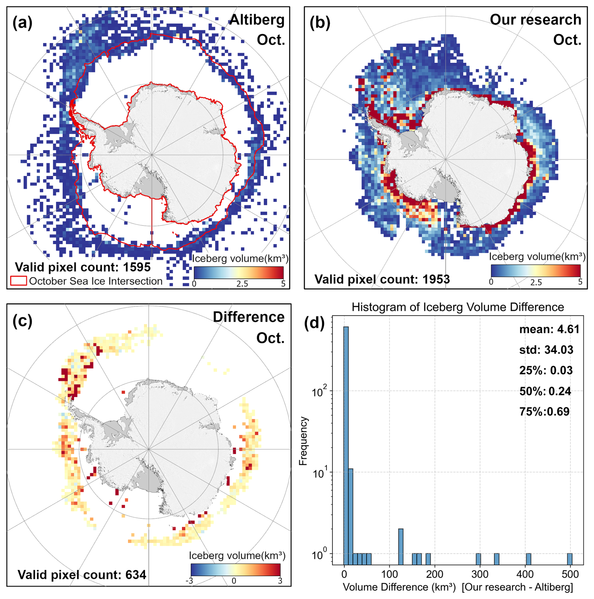
Figure 6 Panel (a) shows the six-year average iceberg volume from the Altiberg database for each October from 2018 to 2023. Panel (b) displays the six-year average iceberg volume from our dataset over the same time period and grid. Panel (c) presents the volume differences (our dataset minus the Altiberg database), and panel (d) summarizes the statistical distribution of these differences.

4.3.3 Comparison with previous studies

Compared with the Antarctic coastal icebergs larger than 0.1 km² identified by Barbet using RAMP data (Barbat et al., 2019b), our dataset covers a broader area and employs a lower threshold for minimum iceberg size, thereby capturing a larger number of icebergs with smaller scales and resulting in certain differences in the overall findings. Relying solely on coastal data tends to underestimate the actual number of small icebergs, because these smaller icebergs are often rapidly transported by wind and coastal currents to the open ocean shortly after formation. Coastal regions mainly record the icebergs released during the initial stages of ice shelf and glacier calving, and due to their small size, small icebergs are more strongly influenced by wind, resulting in a significantly lower proportion in coastal observations. Despite the significant differences in total iceberg numbers between the two studies, as shown in Fig. 7b, the relative proportions of icebergs by size category are generally consistent and exhibit minimal interannual variation, indicating that the size structure of Antarctic icebergs has maintained a certain degree of temporal stability.

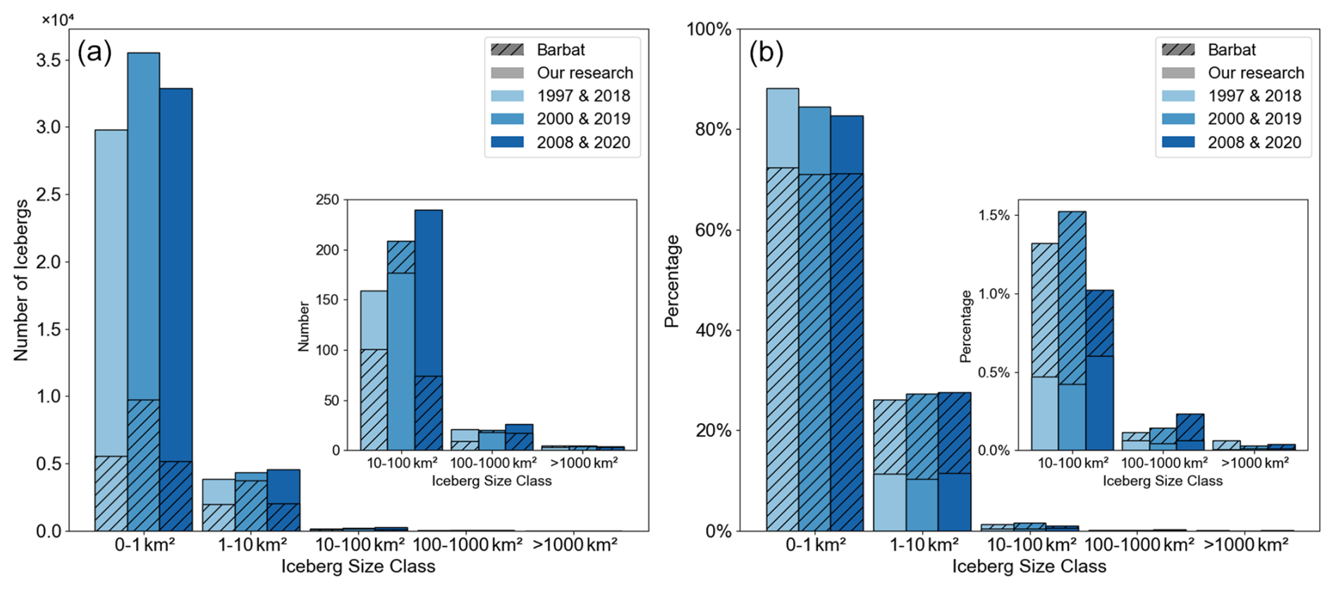
Figure 7 Comparison with the results of Barbat et al. (2019a): (a) Number of Antarctic icebergs and (b) Proportion of different categories.

5 Result and discussion

5.1 Number, area, and mass of circum-Antarctic icebergs

The statistics of circum-Antarctic icebergs from 2018 to 2023 are presented in Table 4, showing significant interannual variations in both iceberg number and area. In 2018, a total of 34 825 icebergs were observed in the circumpolar region, covering an area of 38 668 ± 4645 km². In 2019, the number of icebergs increased to 39 261, and the area rose to 42 001 ± 5103 km². Although the number of icebergs slightly decreased to 38 066 in 2020, the total area continued to increase, reaching 45 959 ± 5258 km². In 2021, both the number of icebergs and their area peaked over the six-year period, with 51 420 icebergs and an area of 52 276 ± 5253 km². In 2022, the number of icebergs dropped to 36 186, and the area decreased to 46 840 ± 4471 km². However, in 2023, the number of icebergs went up again to 44 537, with an area of 43 409 ± 4673 km². The interannual variations in the number and area of icebergs reflect the dynamic nature of the Antarctic ice sheet and its response to climate change. Furthermore, We calculated the intersection of the effective observation areas for each year (Fig. 3) and, based on this intersected area, computed the proportion of icebergs falling within it relative to the total annual iceberg number, as reported in the “percentage” column of Table 4.

Table 4 Total number, area, mass of icebergs and percentage of icebergs in the intersection area in the circum-Antarctic region from 2018 to 2023.

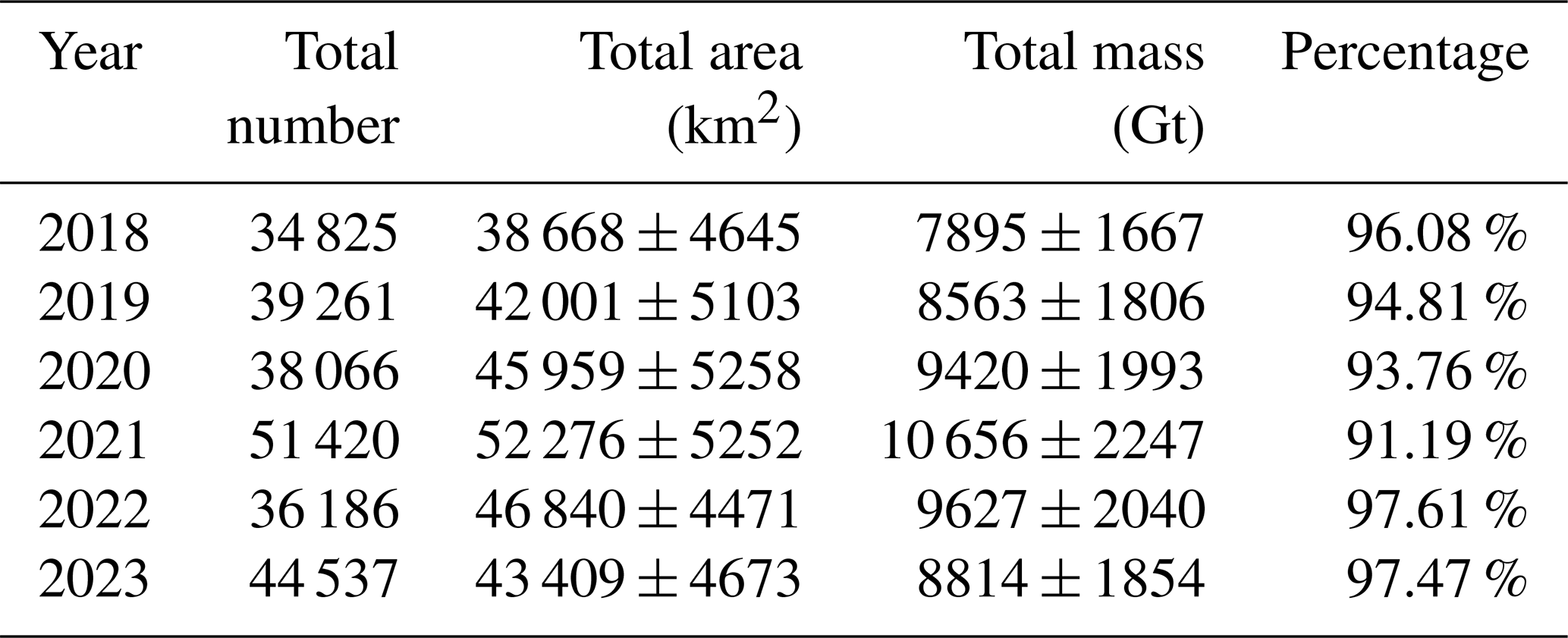
Similar to the interannual variations in iceberg area, the total mass of Antarctic icebergs showed an increasing trend from 2018 to 2021, rising from 7895 ± 1667 Gt in 2018 to 10 656 ± 2247 Gt in 2021, before decreasing to 9627 ± 2040 Gt in 2022 and 8814 ± 1854 Gt in 2023.

5.2 Spatial distribution of icebergs

Figure 8 shows the distribution of icebergs in October for each year from 2018 to 2023. Overall, iceberg density is high at the Thwaites, Dotson, Holmes, Totten, and Mertz ice shelves, indicating that calving activity in these areas is both frequent and intense. In contrast, in large ice shelf regions such as the Ross Sea and Weddell Sea, although calving events occur less frequently from year to year, when a large-scale fracture does occur, it typically leads to the rapid formation of a high-density iceberg zone in a short period. Figure 9 further illustrates the distribution of icebergs by size, showing that medium-to-large icebergs tend to be concentrated in near-coastal waters and are spatially more scattered, whereas small icebergs are widely distributed throughout the Southern Ocean.

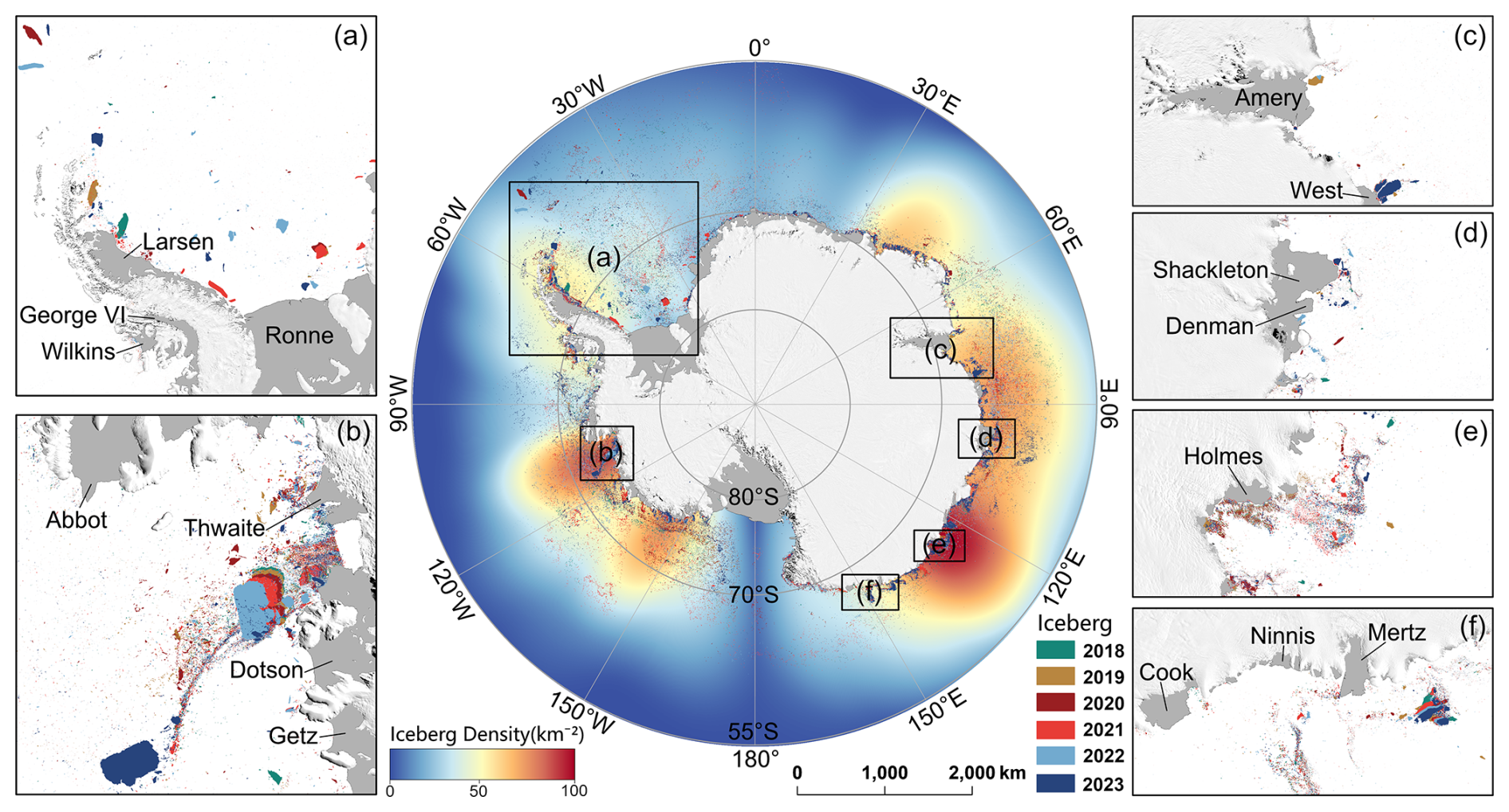
Figure 8 Distribution of Icebergs in the Circum-Antarctic Region from October 2018 to October 2023. The central map represents the distribution of icebergs over the six years, with different colors indicating different years. The base map shows the iceberg density. Panels (a)–(f) display the distribution of icebergs at the front of ice shelves that are prone to calving.

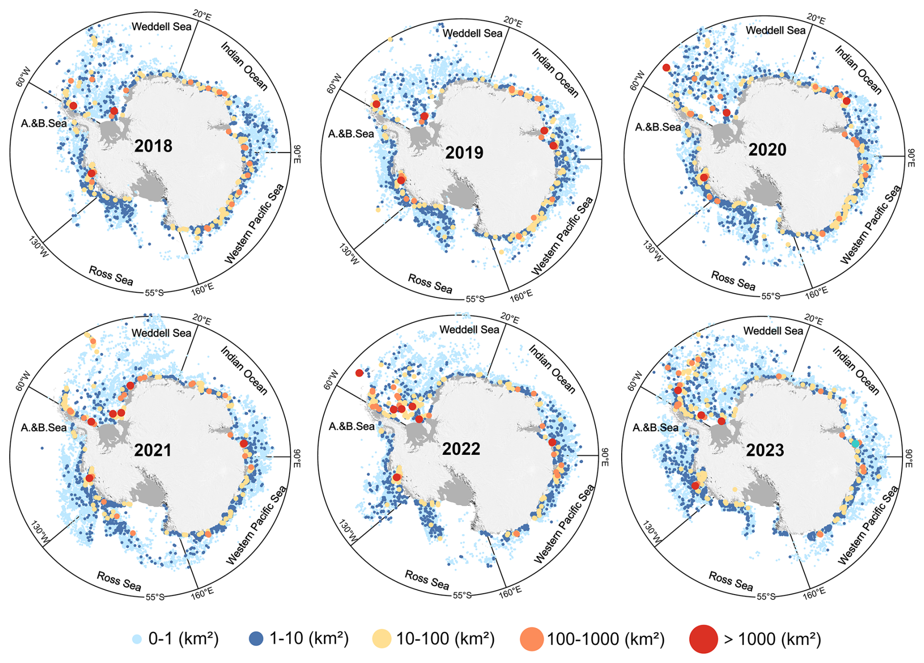
Figure 9 Iceberg counts for different size classes in various sea sectors from 2018 to 2023. Each point represents an individual iceberg, point sizes represent five size categories (A1–A5).

Following Wesche and Dierking (2015)'s rule, all detected icebergs are classified into five size categories, as shown in Fig. 10: A1 (<1 km²), A2 (1–10 km²), A3 (10–100 km²), A4 (100–1000 km²), and A5 (≥1000 km²). From 2018 to 2023, the number of the smallest icebergs (A1) shows significant fluctuations, alternating between increases and decreases and consistently accounting for over 85 % of the total iceberg count, thus driving the overall variability in iceberg numbers. In contrast, the number of medium-sized icebergs (A2 and A3) generally increases, reaching a peak in 2020 before slightly declining; their fluctuations are much smaller compared to those of the A1 category, comprising roughly 10 % of the total. Large icebergs (A4 and A5) are relatively rare, and their occurrence is closely associated with major ice shelf calving events – years such as 2017/18 (A68a), 2019 (D28), 2020(A69) and 2021 (A74 and A76a) see a surge in this size (Braakmann-Folgmann et al., 2022; Deakin et al., 2024). Moreover, small icebergs not only result from continuous small-scale calving but can also originate from the further breakup of large icebergs during their drift. Based on this, although the annual iceberg count is predominantly driven by small icebergs, following a large ice shelf fracture the rapid increase in large icebergs is typically accompanied by their subsequent fragmentation, which in turn leads to an additional rise in the number of small icebergs.

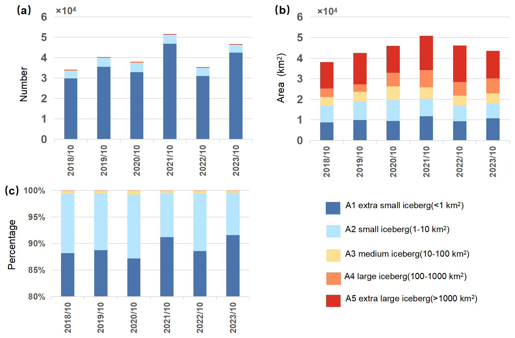
Figure 10 Annual distribution characteristics of Antarctic icebergs in five categories from October 2018 to October 2023. Panels (a)–(c) show the number, area, and percentage of icebergs in each category, respectively. Note that the y axis in (c) is truncated at 80 % for clarity.

To assess the spatial distribution of icebergs, the circumpolar ocean region was divided into five sectors based on longitude: Ross Sea Sector (160° E to 130° W), Amundsen and Bellingshausen Seas Sector (130–60° W), Weddell Sea Sector (60° W to 20° E), Indian Ocean Sector (20–90° E), and Western Pacific Ocean Sector (90–160° E) (Parkinson and Cavalieri, 2012). Figure 11a and b present the number of icebergs and their relative percentages in each sector. The results show that over these six years, the Western Pacific Ocean Sector contributed the highest number of icebergs, while the Weddell Sea Sector recorded the fewest from 2018 to 2021, but in 2022 and 2023 its iceberg count surpassed that of the Ross Sea. In the Ross Sea Sector, the iceberg proportion (i.e., the number of icebergs in the sector as a percentage of the total Southern Ocean iceberg count) remained stable at around 16 % in 2018 and 2019, increased to 21.7 % in 2020, and then rapidly declined to 14 % and 9.8 % in 2021 and 2022, respectively. The proportions in the Indian Ocean and Amundsen and Bellingshausen Seas sectors remained relatively stable at approximately 20 % over the six-year period.

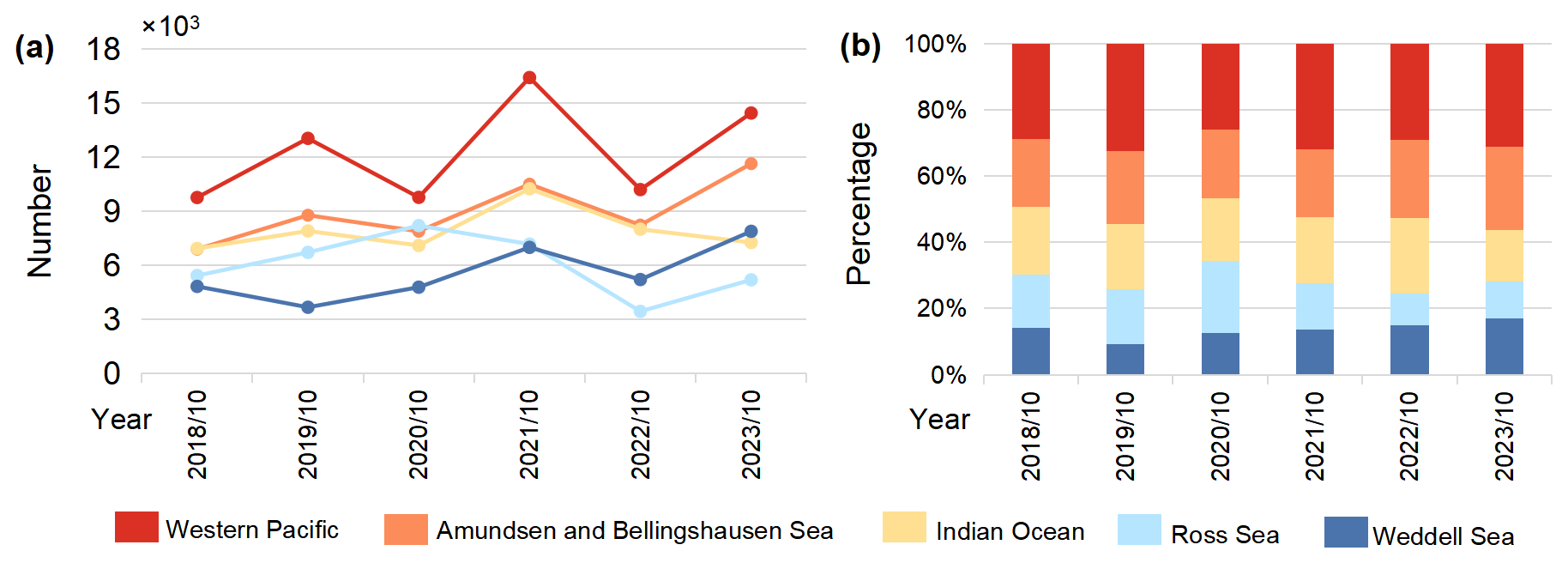
Figure 11 Annual variation trends of icebergs in five major Southern Ocean sectors from October 2018 to October 2023. Panels (a) and (b) present the number and percentage of icebergs of five categories in different sea sectors.

5.3 Distinctive spatial characteristics and formation mechanisms of small-scale icebergs in the Southern Ocean

This study's dataset is unique in both the scales and quantity of icebergs, particularly as it is the first to include small icebergs in the 0.04–0.1 km² size area derived from remote sensing imagery. Over the six-year period, the average number of icebergs in this size range was 8272, accounting for 15.25 % to 29.02 % of the total number each year, with an average area of 559.5 km², contributing 0.97 % to 1.93 % of the total iceberg area.

To examine the spatial distribution and formation mechanisms of these small icebergs, we divided the Southern Ocean into 50 km×50 km grids and calculated the average number of small icebergs in each grid from 2018 to 2023, as well as the average distance between these small icebergs and large icebergs (>100 km²) (Fig. 12). The results show that small icebergs are mainly concentrated at ice shelf fronts, though their distribution is sparse at the fronts of the Ross Ice Shelf, Filchner-Ronne Ice Shelf, and Riiser-Larsen Ice Shelf. Due to their size, these icebergs have short lifespans and are more sensitive to changes in surrounding sea ice and ocean conditions.

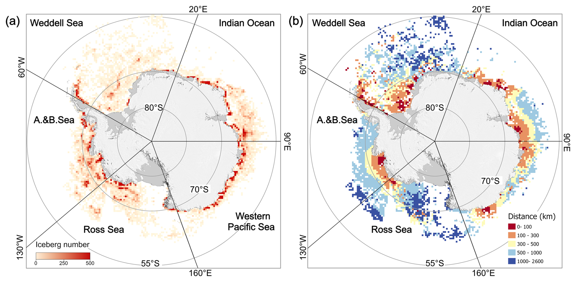
Figure 12 The spatial distribution characteristics of icebergs with sizes between 0.04 and 0.1 km² in 50 km×50 km grids in the Southern Ocean. Panel (a) represents the average number of icebergs in each grid cell from 2018 to 2023; Panel (b) shows the average distance from the icebergs in each grid to the nearest large iceberg (area greater than 100 km²).

In analyzing the distances between small and large icebergs, we further derived conclusions consistent with the small-iceberg formation mechanism proposed by Tournadre et al. (2016). The results indicate that small icebergs in the Southern Ocean follow two main patterns: one where small icebergs are found near large icebergs, suggesting they may originate from fragmentation, share a common source, or drift along similar paths; and another where small icebergs exhibit “free drift,” unrelated to any large icebergs, drifting far from their calving sources, such as in the Ross Sea, Bellingshausen Sea, and eastern Weddell Sea. In these regions, the drift of small icebergs plays a key role in transporting ice shelf and large iceberg material, significantly influencing regional ice flow and freshwater flux. The drift paths can extend thousands of kilometers, forming independent “drifting alley”.

6 Code and data availability

The GEE code for data acquisition, the MATLAB code for image segmentation, feature extraction, and the dataset of icebergs outlines in shapefile format along with their latitude and longitude, area, perimeter, and other attribute information, are all available at https://doi.org/10.5281/zenodo.17165466 (Liu and Chen, 2025).

7 Conclusions

This study successfully identified circum-Antarctic icebergs from 2018 to 2023 using Sentinel-1 SAR mosaic data obtained from the Google Earth Engine (GEE) platform, combined with an incremental random forest algorithm and manual corrections. The smallest identifiable iceberg had an area of 0.04 km². This is the first high-precision dataset covering the entire Southern Ocean, including small icebergs. Small icebergs dominate in terms of quantity, and their distribution is critical for initializing coupled ocean-iceberg models, aiding in more accurate simulations of iceberg melting effects on ocean circulation and global climate.

Although this study primarily used data from October each year, when the difference in backscatter characteristics between icebergs and other oceanic features is most pronounced, and the identification results are optimal, the method is not limited to this period. In the future, images from other months can be obtained via the GEE platform, enabling the study of seasonal variations and year-round iceberg dynamics. This approach compensates for the limitations of snapshot data, providing a more comprehensive understanding of iceberg formation, drift, and melting processes.

Despite the extensive coverage of Sentinel-1 SAR data, data gaps existed in certain years and regions, such as in parts of the Indian Ocean in 2018, which may have led to an underestimation of iceberg numbers in these areas. In terms of mass estimation, the adopted parameterization constrains small icebergs through an area-volume scaling and assumes a fixed maximum thickness of 250 m for large icebergs. These simplifications do not fully capture the variability in iceberg geometry, calving source, or melt state, and may therefore introduce biases (Dowdeswell and Bamber, 2007). Furthermore, Although we employed a high-precision iceberg identification model supplemented by manual corrections within a semi-automated workflow, in complex marine and terrestrial environments (e.g., regions with dense sea ice and iceberg calving zones), the radar signals of icebergs are often weak and their boundaries blurred due to noise and adverse sea conditions, potentially resulting in varying degrees of omissions, erroneous merging, and contour deviations. Future research could consider integrating multi-source remote sensing data and incorporating more advanced deep learning algorithms to further improve iceberg identification accuracy.

Overall, this study provides the first high-precision iceberg distribution dataset for the Southern Ocean, including small icebergs. It lays the foundation for a deeper understanding of the impact of icebergs on the marine environment and global climate and offers valuable data support for future research. Moving forward, we plan to use imagery from additional months to study seasonal and interannual variations in iceberg distribution and their long-term impacts on marine ecosystems and climate systems. Besides, we attempt to backtrack and update this product as a “living” dataset, meaning it will be continuously updated and expanded as new input observations available, such as Sentinel-1A/B before 2018 and Sentinel-1C after 2024.

Appendix A: Feature description

Table A1 Feature Categories and Descriptions.

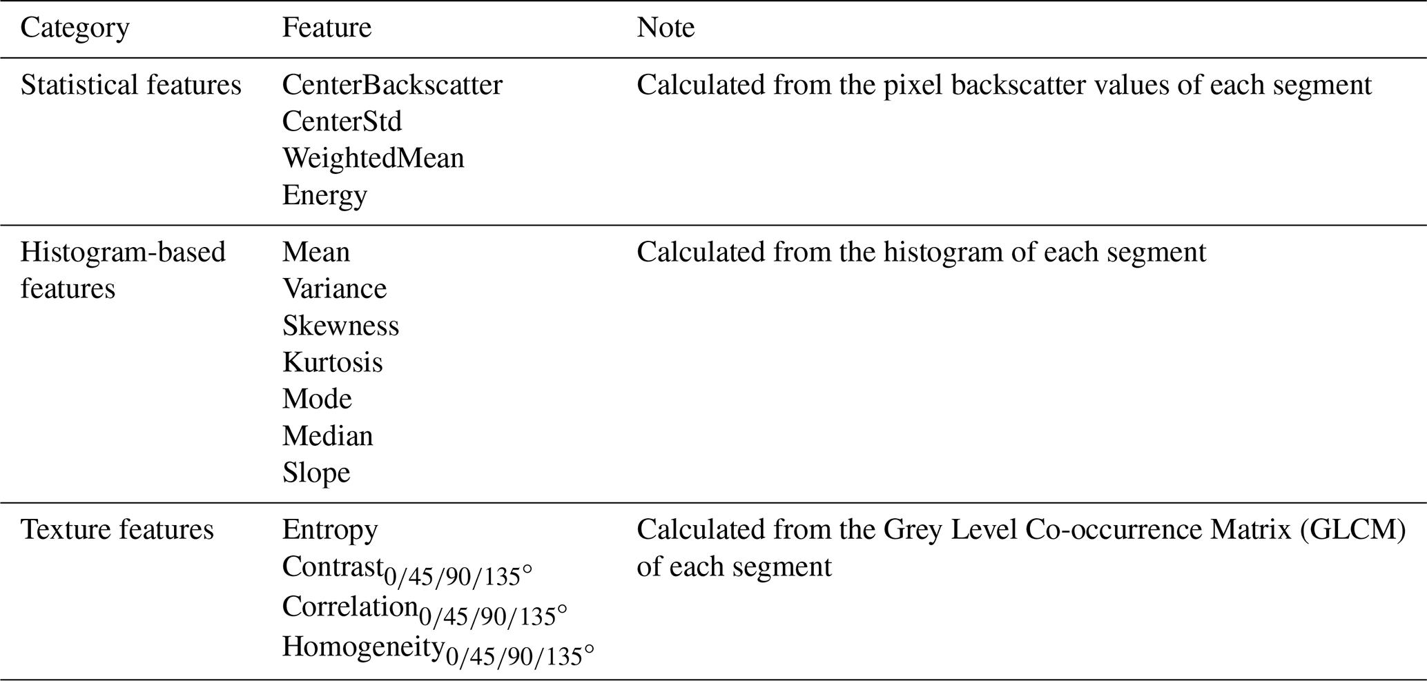
(1) Statistical features: Calculated from the pixel backscatter values of each segment

1. CenterBackscatter: The grayscale value at the center position of the superpixel object. A superpixel is defined as a small, contiguous cluster of adjacent pixels that share similar backscatter characteristics, effectively representing a meaningful image region rather than individual pixels.

2. CenterStd: The standard deviation within a 3×3 range near the center of the superpixel. If there are fewer than 3×3 pixels around the center, then CenterStd=0.

3. WeightedMean: Obtained from Eq. (A1):

   $$\begin{array}{}\text{(A1)}& \text{WeightedMean}=\sum _{ij}{\displaystyle \frac{\mathrm{1}}{D_{ij}}}{x}_{ij}\end{array}$$

   where x_ij is the grayscale of the pixel at position (i,j), and D_ij is the distance from that pixel to the centroid of the superpixel.

4. Energy: Obtained from Eq. (A2):

   $$\begin{array}{}\text{(A2)}& \text{Energy}={\displaystyle \frac{\mathrm{1}}{N}}\sum _{ij}{x}_{ij}^{\mathrm{2}}\end{array}$$

   where N is the total number of pixels within the superpixel.

(2) Histogram-based features (bin=0.1): Calculated from the histogram of each segment

1. Mean. The average of all pixel grayscale values within the superpixel.

2. Variance. The variance of all pixel grayscale values within the superpixel.

3. Skewness. Used to measure the asymmetry of the histogram distribution of grayscale values of all pixels within a superpixel.It can derived from the Eq. (A3):

   $$\begin{array}{}\text{(A3)}& \text{Skewness}=E\left[{\left({\displaystyle \frac{x-\mathit{\mu }}{\mathit{\sigma }}}\right)}^{\mathrm{3}}\right]\end{array}$$

4. Kurtosis. Characterizes the height of the peak at the mean of the probability distribution curve, that is, the shape of the curve's peak. The larger the kurtosis, the sharper the peak.

   $$\begin{array}{}\text{(A4)}& \text{Kurtosis}=E\left[{\left({\displaystyle \frac{x-\mathit{\mu }}{\mathit{\sigma }}}\right)}^{\mathrm{4}}\right]\end{array}$$

5. Mode. The most frequent value in the grayscale values of the superpixel. If multiple values occur with the same frequency, the Mode is the smallest of these values.

6. Median. The median of the grayscale values of all pixels within the superpixel.

7. Slope. The one-sided slope of the probability distribution curve.

   $$\begin{array}{}\text{(A5)}& \text{Slope}={\tan }^{-\mathrm{1}}\left({\displaystyle \frac{P\left(M\right)}{max\left(x\right)-M}}\right)\end{array}$$

   Where M is the median of the grayscale values, and P(M) is the probability density corresponding to the median.

(3) Texture features: Calculated from the Grey Level Co-occurrence Matrix(GLCM) of each segment

1. Entropy. It characterizes the overall distribution of grayscale values in the image.

   $$\begin{array}{}\text{(A6)}& \text{Entropy}=-\sum _{n}P\left(i\right)\cdot {\log }_{\mathrm{2}}P\left(i\right)\end{array}$$

   where n is the number of grayscale levels obtained by binning the histogram of all pixel grayscale values within a superpixel with bin=0.1, and P(i) is the probability density value corresponding to the ith grayscale level.

2. Contrast${}_{\mathrm{0}/\mathrm{45}/\mathrm{90}/\mathrm{135}\mathit{°}}$

3. Correlation${}_{\mathrm{0}/\mathrm{45}/\mathrm{90}/\mathrm{135}\mathit{°}}$

4. Homogeneity${}_{\mathrm{0}/\mathrm{45}/\mathrm{90}/\mathrm{135}\mathit{°}}$

   In our research, the Gray-Level Co-Occurrence Matrix (GLCM) is used to calculate the texture features of superpixels. The GLCM characterizes the texture of an image by calculating the frequency of occurrence of pixel pairs with specific values and spatial relationships in the image (Haralick et al., 1973). The elements of the Gray-Level Co-Occurrence Matrix are calculated using the Eq. (A7):

   $$\begin{array}{}\text{(A7)}& P(i,j)={\displaystyle \frac{P(i,j,d,\mathit{\theta })}{{\sum }_i{\sum }_{j}P(i,j,d,\mathit{\theta })}}\end{array}$$

   The element P(i,j) in the matrix represents the probability of the occurrence of pixel pairs at a distance d in the direction θ. In this study, we consider the GLCM for the cases when d=0 and θ=0, 45, 90, 135°. For non-rectangular superpixels, missing pixels are filled with 0. After calculating the GLCM for each superpixel in these four directions, we can further compute metrics that describe contrast, correlation, and homogeneity. The equation is as follows:

   $$\begin{array}{}\text{(A8)}& {\displaystyle }\text{Contrast}=\sum _{i,j}(i-j{)}^{\mathrm{2}}P(i,j)\text{(A9)}& {\displaystyle }\text{Correlation}=\sum _{i,j}{\displaystyle \frac{(i-{\mathit{\mu }}_i)(j-{\mathit{\mu }}_j)P(i,j)}{{\mathit{\sigma }}_i{\mathit{\sigma }}_j}}\text{(A10)}& {\displaystyle }\text{Homogeneity}=\sum _{i,j}{\displaystyle \frac{P(i,j)}{\mathrm{1}+(i-j{)}^{\mathrm{2}}}}\end{array}$$