An observational record of global gridded near-surface air temperature change over land and ocean from 1781

We present a new gridded data set of air temperature change across global land and ocean extending back to the 1780s. This data set, called the GloSAT reference analysis, has two novel features: it uses marine air temperature observations rather than the sea surface temperature measurements typically used by pre-existing data sets, and it extends further into the past than existing merged land and ocean instrumental temperature records which typically estimate temperature changes from the middle to late 19th century onwards. New estimates of diurnal-heating biases in marine air temperatures have enabled the use of daytime observations, extending the data set further into the past compared to nighttime-only marine air temperature data. The data set uses an extended version of the CRUTEM5 station database over land areas, incorporating newly available bias adjustments for non-standard thermometer enclosures used prior to the adoption of Stevenson screens and new climatological normal estimates for stations with limited data in the 1961–1990 baseline period. Land and marine temperature anomalies are combined to produce a gridded data set following the methods developed for HadCRUT5. The GloSAT global and hemispheric temperature anomaly series show close agreement with those based on sea surface temperature for much of the overlapping period of their records but with slightly less warming overall. The GloSAT reference analysis is available from https://doi.org/10.5285/a2519624a593402a83246bd359d098be (Morice et al., 2025b), the GloSATLAT data set is available from https://doi.org/10.5285/ef237f578329487eb02fb42f9db56bb2 (Morice et al., 2025a), and the GloSATMAT data set is available from https://doi.org/10.5285/e6251bf935304cfbb9c9269dc7757a35 (Cornes et al., 2025b).

1 Introduction

Instrumental data sets recording changes and variations in near-surface temperature across the globe have been widely used to monitor changes in global and regional climate (World Meteorological Organisation, 2023). The Intergovernmental Panel on Climate Change 6th Assessment Report (IPCC AR6) assessment of global average temperature change from the mid-19th century (Gulev et al., 2021) is underpinned by instrumental data sets that combine information from sea surface temperature (SST) observations with information from meteorological station observations of land surface air temperature (LSAT). The IPCC AR6 refers to changes in mean near-surface temperature based on this combination of SST and LSAT as the global mean surface temperature (GMST). Studies using climate model output commonly assess changes in near-surface temperature using air temperature changes over both land and ocean, using marine air temperature (MAT) rather than SST. The IPCC AR6 refers to this combination of LSAT and MAT as global surface air temperature (GSAT). Hence, the difference between GMST and GSAT is the use of SST or MAT to measure changes over the marine regions.

Existing global instrumental data sets used to monitor changes in GMST combine measurements of near-surface air temperatures at meteorological stations (LSATs) with measurements of surface water temperatures obtained by ships, buoys, and moorings (SSTs). The currently available data sets of this type include HadCRUT5 (Morice et al., 2021), GISTEMP (Lenssen et al., 2019), NOAAGlobalTemp (Yin et al., 2024; Huang et al., 2022), Berkeley Earth (Rohde and Hausfather, 2020), Kadow et al. (Kadow et al., 2020), CMST 2.0 (Sun et al., 2022), DCENT (Chan et al., 2024), Calvert (Calvert, 2024), and COBE-STEMP3 (Ishii et al., 2025). Each of these data sets provides global grids that map GMST variability and change along with derived global and regional average time series. These data products have starting dates ranging from 1850 to 1880 as data availability, particularly with regard to SST and over land in the Southern Hemisphere, decreases rapidly prior to this.

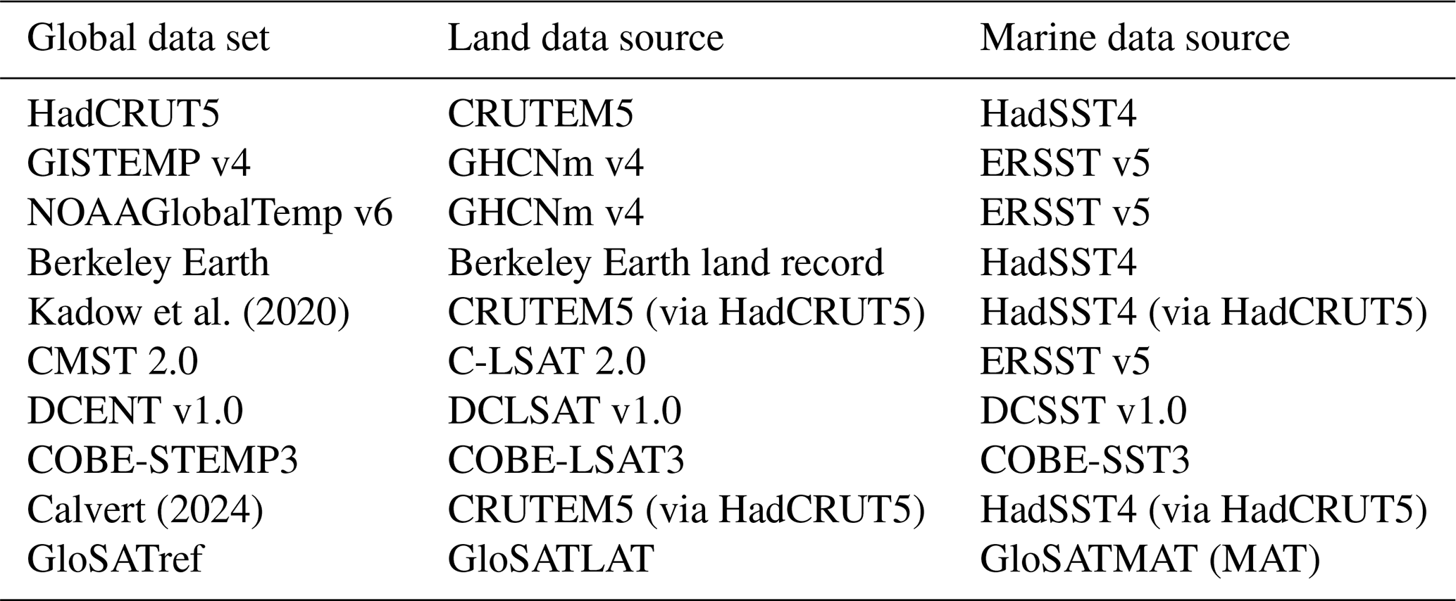
Data sources for current observational surface temperature data sets are shown in Table 1. There are many common observational data underpinning the named LSAT and SST data sets because of global data sharing and consolidation of national records into global archives. For example, the International Comprehensive Ocean-Atmosphere Data Set (ICOADS) (Freeman et al., 2017) is an underpinning source for each of the marine data sets in Table 1. Despite these overlaps in observation sources, there are differences in terms of the selection criteria used in each data set, and sometimes standard data holdings are extended, e.g., through the addition of newly digitized historical sources. Each data set also differs in terms of some or all of the methods for data quality control (QC), the methods used to account for systematic changes in observing practices, the gridding methods, and uncertainty modelling. Some data sets have independent processing workflows, such as NOAAGlobalTemp v6 and HadCRUT5. Others share aspects of processing, such as the reprocessing of HadCRUT5 data using alternative gridding methods by Kadow et al. (2020) and alternative gridding methods and bias adjustment in Calvert (2024). The eight currently updated GMST data sets each use a combination of one of five LSAT data sets and one of three SST data sets (Table 1).

Kadow et al. (2020)Calvert (2024)

Table 1 Global instrumental data sets reporting GMST and their land and marine data sources. LSAT data sets: CRUTEM5 (Osborn et al., 2021), GHCNm v4 (Menne et al., 2018), Berkeley Earth land record (Rohde et al., 2013a, b), C-LSAT 2.0 (Li et al., 2021), and DCLSAT v1.0 (Chan et al., 2024). SST data sets: HadSST4 (Kennedy et al., 2019), ERSST v5 (Huang et al., 2017), DCSST v1.0 (Chan et al., 2024), and COBE-STEMP3 (Ishii et al., 2025). All land data sources are LSAT data sets. All marine data sources are SST data sets, except for GloSATMAT, used in GloSATref, which is an all-hour MAT data set.

Historically, SST rather than MAT has been used in global temperature products for three main reasons (Jones et al., 1999): (1) there are substantially fewer MAT observations available from approximately 1900 onwards, (2) there are diurnal-heating biases in the MAT data that require adjustment, and (3) adjustment of MAT measurements to a common reference height are required to account for changes in measurement heights throughout the MAT record. SST observations are also affected by sampling limitations and systematic changes in measurement practices (Kennedy et al., 2019; Kent and Kennedy, 2021), but the adjustments required for MAT records were considered to be more complex and uncertain (Rayner et al., 2003). Furthermore, while a decline in ship coverage has resulted in fewer observations of both SST and MAT since the 1960s, in the case of SST, this has been mitigated through the increasing coverage of drifting-buoy and satellite data (Kent and Kennedy, 2021).

Nighttime marine air temperature (NMAT) observations have previously been used to avoid the need to make diurnal-heating bias corrections and are available from CLASSnmat (Cornes et al., 2020a) and UAHNMATv1 (Junod and Christy, 2020). Both ERSST v5 and HadSST4 use NMAT observations within their SST bias adjustment methods. ERSST v5 uses NMAT–SST differences to derive a bias adjustment that is applied to ship SST observations prior to 2010. The HadSST4 bias adjustment model uses NMAT–SST differences to constrain the estimates of contributions of different measurement types for observations made from 1850 to 1920. These NMAT data sets have not previously been combined with LSAT to create GSAT data sets.

The IPCC AR6 (Gulev et al., 2021) reviewed whether differences between GMST and GSAT reconstructions should be expected. This included a review of a range of model-based studies and process understanding and differences between instrumental NMAT and SST data sets. Differences between the two diagnostics have been the subject of recent debate due to the common (but not exclusive) use of GSAT to assess near-surface temperature changes in climate models, while observational records have been based on GMST. Studies investigating differences between GMST and GSAT diagnostics have included physical reasoning (Richardson, 2023) and have assessed the impact of the choices of methods used to merge SST and LSAT data (Cowtan et al., 2015; Jones, 2020; Richardson et al., 2018), particularly in regions of changing sea ice cover (Cowtan et al., 2015; Richardson et al., 2018). The IPCC AR6 concluded that “There is high confidence that long-term changes in GMST and GSAT differ by at most 10 % in either direction” with “low confidence in the sign of any difference in long term trends” (IPCC WG1 Cross-Chapter Box 2.3) (Gulev et al., 2021). Based on this understanding and with no available instrumental GSAT data set, the IPCC AR6 derived estimates of GSAT change equal to the change in observed GMST, with expanded uncertainty ranges to account for differences between the two diagnostics.

This article describes a new gridded surface air temperature (SAT) data set, the GloSAT reference analysis (GloSATref.1.0.0.0, hereafter referred to as GloSATref). The data set adds to the available set of estimates of global surface temperature in several ways. Firstly, the use of MAT enables an extension of the instrumental record prior to the start of systematic SST observation in the 1850s. Secondly, this earlier extension requires adjustments for the effects of solar heating of the measurements, with adjustments having been developed for both marine and land observations and applied in GloSAT. Thirdly, because climate models show different evolutions of GMST and GSAT, improving our instrumental records of both measures will help inform ongoing discussions about resolving the disagreements between methods and data sets. Finally, SST and MAT observations contain different biases, and so producing analyses based on both measures samples another dimension of the structural uncertainty inherent in estimates of global surface temperature. The name “reference analysis” is adopted because the data set is intended to provide a reference for the comparison of observed GMST and GSAT, with processing based on the processing workflow of the HadCRUT5 GMST data set (Morice et al., 2021).

The new data set combines an extended and improved version of the CRUTEM5 LSAT database, updated from Osborn et al. (2021), with a new MAT data set based on all-hour observations, building on Cornes et al. (2020a). Section 2 describes the processing of input LSAT and MAT data sets and their use in constructing the combined GloSATref analysis, following the processing workflow of Morice et al. (2021). Section 3 presents global and regional climate diagnostics derived from the merged SAT analysis. Conclusions are presented in Sect. 5.

2 Methods for producing the GloSAT data set

2.1 Land surface air temperature data processing

The GloSAT reference analysis (GloSATref) uses an updated database of monthly average air temperature at surface meteorological stations. This is an extended version of the CRUTEM5 station database (Osborn et al., 2021), including additional station data, updated methods for climatological normal calculation (Taylor et al., 2025), and new bias adjustments for early instrumental measurements prior to the adoption of louvred Stevenson-style screens (Wallis et al., 2024). The following subsections describe the land station data contributing to the GloSATref analysis.

2.1.1 Land station data acquisitions and quality control

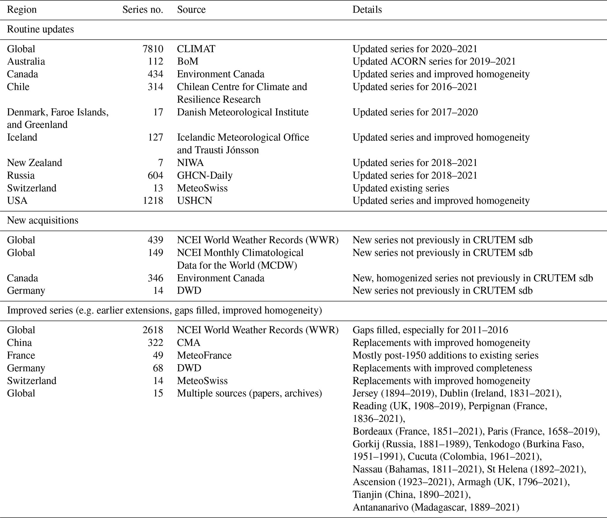
The new acquisitions and improved/updated series are summarized in Table 2. Quality control is applied to these data at the source by the national meteorological services together with further quality control following the methods described in Osborn et al. (2021). These include station neighbours and station extreme-threshold checks, with threshold modifications based on neighbour stations, and the identification and removal of physically implausible values (taking into account the month of the year, station elevation, and station latitude).

Table 2 Summary of new acquisitions and updates applied to CRUTEM.5.0.1.0 to create the GloSAT land surface air temperature station database (sdb). Place and country names are as given by the data source.

2.1.2 Early-record exposure biases

Measurements in the early record were made in thermometer shelters of widely varying designs. Disparities between measurements made using these different shelters were already being noted in the mid-19th century (Naylor, 2018), and the process of understanding those differences and the more general difficulties of making reliable and practical measurements across a global network of observers led, eventually, to standards for the siting and design of instrument shelters such as those provided by the World Meteorological Organisation (WMO, 2018). The transition from non-standard shelters to Stevenson-style screens is a known source of systematic bias – called exposure bias – because earlier shelters were subject to differences in ventilation and direct or indirect radiative heating of the thermometer. Resulting biases exhibit a seasonal structure with an identifiable impact on regional trends (Parker, 1994).

Current global data sets do not explicitly account for exposure bias across their networks of station data. Some (e.g. Berkeley Earth land record or those using GHCNm v4; see Table 1) rely on their general statistical homogenization algorithms to detect and adjust for breakpoints arising from exposure changes. These are not specifically designed for identifying exposure biases, but where those biases are detected, they may yield a similar outcome. However, the power of breakpoint detection is reduced if changes in exposure were introduced within the same time frame across many stations within a country or region (Menne and Williams, 2009), which was often the case for the introduction of Stevenson screens (Wallis et al., 2024). Other data sets leave exposure biases mostly uncorrected and instead represent their effects via a component in their uncertainty model, developed from previous exposure bias assessments (Brohan et al., 2006; Morice et al., 2012). Only a limited number of data sources have explicitly adjusted for exposure biases in early temperature records; e.g. in CRUTEM5, only some data sources for Spain (Brunet et al., 2006, 2011), the Greater Alpine Region (Böhm et al., 2009), and Australia (Ashcroft et al., 2014) have had adjustments applied. Specific exposure bias adjustments have not been developed and applied more widely because quantitative estimates of the bias and comprehensive metadata describing screen types in terms of use over time at each meteorological station have been lacking.

Wallis et al. (2024) made a significant step forward in addressing these gaps by compiling temperature observations from 54 parallel measurement series at sites where multiple thermometer shelters were simultaneously in operation and using them to develop regression-based predictive models of the bias between measurements taken in Stevenson-style screens versus those taken in earlier shelters. These regression models were selected and calibrated using parallel measurements for four classes of shelter:

• open exposures that, barring shielding to the top and one side, fully expose the thermometer to the air, including Glaisher and Montsouris stands (bias predictors are annual temperature and a climatology of surface solar radiation);

• intermediate exposures that provide additional lateral protection to the thermometer, including thermometer sheds and summer houses (this bias prediction model was not applied because its skill arose mostly from a single parallel measurement site);

• closed exposures in which the thermometer is fully shielded on all sides, including Wild huts (the bias predictor is a climatology of surface solar radiation);

• wall-mounted exposures, including wall-, fence-, or window-mounted measurements, both screened and unscreened (the bias predictor is the top-of-atmosphere downward solar radiation).

Wallis et al. (2024) then compiled a database of shelter types for the majority of mid-latitude stations that had some pre-1961 data in the GloSAT station database. These metadata provide an estimate of the shelter types in use up to the time that a Stevenson-style screen was introduced and allow for a prediction of the exposure bias arising from the transition from these earlier shelters to the Stevenson-style screen using the aforementioned regression models.

The bias estimates from Wallis et al. (2024) have been applied here to adjust the GloSAT station database for exposure bias. Of the 5031 stations between 30° and 60° latitude (in either hemisphere) with some data prior to 1961, exposure bias was considered to be absent in 1898 stations (either because they had already been adjusted or because the metadata suggest that a Stevenson screen had been in place from the start of the record). Of the remaining 3133 stations, new exposure bias adjustments were applied to 1960 stations. No adjustments were made to 1173 stations either because shelter metadata were absent or because Wallis et al. (2024) had not found an acceptable bias prediction model (e.g. for intermediate exposures).

Even though we apply these new adjustments for exposure bias, we retain the exposure bias error term in the Morice et al. (2012) uncertainty model without any reduction. This provides conservative bounds on remaining exposure-related uncertainty in regional and global averages and is appropriate because residual exposure biases are still present in the GloSAT station database (from those tropical and high-latitude stations not assessed by Wallis et al. (2024) or lacking necessary metadata or due to transitions from very early exposures that have not been considered).

2.1.3 Improved and additional station normals

The GloSATref gridding process requires the monthly temperatures to be expressed as anomalies by subtracting an estimate of each station's average (hereafter “station normal”) during the 1961–1990 baseline. In CRUTEM5 (Osborn et al., 2021), station normals were computed for each calendar month where at least 15 out of 30 years of data were available in the 1961–1990 period. For stations where this criterion was not met, some station normals were obtained from the WMO (World Meteorological Organisation, 1996) or were estimated by computing 1951–1970 normals, which were then adjusted to represent the 1961–1990 mean based on the difference between the grid box averages for 1961–1990 and 1951–1970 at nearby locations (Jones et al., 2012; Jones and Moberg, 2003). Applying this approach for the GloSAT reference analysis would have led to 2699 stations being unused due to the absence of an estimated normal and the fact that some estimated normals would have greater uncertainty and small biases (Calvert, 2024; Taylor et al., 2025) due to being estimated from incomplete data.

For the GloSAT reference analysis, therefore, the CRUTEM5 approach is revised to augment the available station observations with individual monthly values estimated by the local-expectation Kriging (LEK) method described by Taylor et al. (2025). The local expectation at a given station location is estimated as a linear weighted average of the temperature values recorded at other stations in the neighbourhood, with the weightings determined by an approximation to Kriging with hold out and taking into account the covariance between stations. The monthly values estimated by LEK are used to fill in missing values within each station time series but only for the purpose of calculating station normals from complete 1961–1990 values. Taylor et al. (2025) evaluate these LEK-estimated normals against normals calculated directly from observed values (for those stations with adequate data during 1961–1990) and find a root-mean-squared difference of approximately 0.2 °C, with no systematic dependence on latitude. This measure of similarity is representative only of stations with data close to the baseline period. For station data fragments further away (in time) from 1961–1990, the normals based on LEK are more uncertain, though this is difficult to quantify; comparison with simple neighbour averages suggests that the uncertainty of those normals may be twice as large as for stations with data close to 1961–1990. The new data set applies the pre-existing HadCRUT uncertainty model for extrapolated normals to those based on LEK, assigning them a larger error than for those calculated from complete 1961–1990 data.

For GloSATref, the normals are therefore calculated either from complete 1961–1990 observations (5806 stations), from a mixed set of observed and LEK-estimated values during 1961–1990 (3568 stations, with reduced bias for cases where the observed values were either at the start or end of the baseline period), or from only LEK-estimated values (1742 stations, typically short-segment stations during earlier or very recent periods). This permits the use of station series for which few or no observations are available in the 1961–1990 period and reduces the use of less reliable WMO normals.

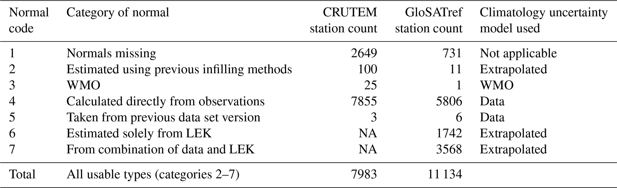
In addition to extending the record back to 1781, the total number of stations in the database is increased from 10 632 in CRUTEM.5.0.1.0 to 11 865 in the GloSAT land station database. The number of stations with normals – and, thus, the number of stations able to be used to create the gridded data set – is increased from 7983 stations in CRUTEM.5.0.1.0 to 11 134 stations for GloSATref.1.0.0.0 (Table 3). Together with new data acquisitions, the use of LEK-derived normals increases the number of usable stations. Many of the stations with new normal information are, however, situated in relatively well-observed locations and cover relatively short periods of time (mean station length is 35 years for those with normals fully or partially calculated from LEK estimates versus 94 years for those with full 1961–1990 data); hence, the spatial coverage of the globe is not increased commensurately with the increased number of stations with climatological normal estimates.

Table 3 Station counts per normal category code in CRUTEM5 and GloSATref. Of those stations coded as have missing normals, 26 do have a normal in up to 5 calendar months. Climatology uncertainty models for data-derived, WMO, and extrapolated normals are described in Brohan et al. (2006) and Morice et al. (2012). Note that NA represents not applicable.

2.2 Marine air temperature data processing

This section describes the processing used to construct a 200-member ensemble of gridded MAT fields that forms the input into the GloSATref spatial analysis. We refer to this MAT data set as GloSATMAT. The production of stable GSAT climate records requires assessment of the systematic biases and uncertainty in MAT observations. The most important of these are diurnal biases and measurement height changes.

Spurious diurnal effects are caused by solar heating of the ship which, in turn, warms the air around the sensor, and these have been addressed previously through two approaches. The first and most common approach is to discard all observations affected by daytime heating to produce a nighttime marine air temperature (NMAT) data set (Bottomley et al., 1990; Cornes et al., 2020a; Junod and Christy, 2020; Kent et al., 2013; Rayner et al., 2003), with the definition of nighttime typically being from 1 h after sunset to 1 h after sunrise. Although simple to apply, this restricts the starting date of NMAT data sets to the late 19th century as, before that time, an increasing proportion of observations were taken during the daytime and, commonly, at local noon (Kent and Kennedy, 2021). The second approach is to model and adjust for daytime biases. This has the advantage of increasing the sample size of observations and was the approach taken by Berry and Kent (2011), who produced a global gridded all-hour air temperature product starting in the 1970s. This approach is also taken here but is used to construct an MAT data set back to 1784. As noted by Berry et al. (2004) and Cropper et al. (2023), this adjustment approach acts on average to remove any real diurnal cycle from the MAT observations. Whilst this is not an ideal solution, this is a pragmatic approach that can be assessed by the similarity between data sets based on MAT and NMAT. Adjustments from the measurement height to a standard reference height are required as the temperature typically decreases with increasing height above the ocean as the sea is usually warmer than the air above. Height adjustments have been made by estimating the lapse rate of the lower atmospheric boundary and using this information with known values (or estimates) of the temperature recording height to adjust the temperature to a common reference height.

Processing of GloSATMAT largely follows Cornes et al. (2020a), with the following description of the method focusing on additions to and variations of that approach. The most notable changes are as follows:

• a refined quality control (QC) procedure;

• development of an ensemble version of the Cornes et al. (2020a) error model to produce a 200-member ensemble data set;

• the inclusion of observations of marine air temperature made during the daytime, following adjustment for daytime heating bias (Cropper et al., 2023) using the method proposed by Berry et al. (2004).

A new version of CLASSnmat (version 2.1.0.2) has also been produced (Cornes et al., 2025a), which uses the same input data and methodology as GloSATMAT but is constructed from nighttime-only values and hence omits the diurnal adjustments. CLASSnmat v2 only extends back to 1880 due to the reduced sampling of nighttime observations before that time.

2.2.1 Marine observations and quality control

The principal source of ship data is the International Comprehensive Ocean-Atmosphere Data Set (ICOADS, Freeman et al., 2017; Li et al., 2021), and data are processed from 1784 to present using the methods described in Cornes et al. (2020a). In addition, ship data from the following sources are also included:

• citizen science data digitization undertaken under the Old Weather initiative (Spencer et al., 2019);

• research vessel data from ICOADS holdings of the Ship-based Automated Meteorological and Oceanographic System (SAMOS) archive (Smith et al., 2018);

• Voluntary Observing Ship Global Data Assembly Centre (VOS-GDAC) data, obtained on 19 January 2021 https://www.dwd.de/EN/ourservices/gcc/gcc.html (last access: 19 January 2021) – in cases where an observation in ICOADS has the same ID, date, and position as a VOS-GDAC observation, the information from the VOS-GDAC observation is used.

As in Kent et al. (2013) and Cornes et al. (2020a), data for the period of 1876–1893 for ships passing through the Suez Canal were excluded due to the warm bias in those observations.

The QC checks applied to the MAT data follow those described in Cornes et al. (2020a). An updated climatology-based quality control check has been developed for the MAT data and is described below. For GloSATMAT, additional checks have been made in relation to the diurnal-heating bias adjustments (Cropper et al., 2023).

Climatology QC procedure

At the start of marine data processing, climatological outliers are rejected based on the climatology generation step. Under the new procedure, a 1961–1990 pentad (5 d) climatology is generated on a 1° latitude × 1° longitude resolution grid. Due to the sampling frequency of ship-based observations, if a grid cell does not initially contain at least one value in each pentad throughout the year or one value in each month then the size of the grid cell, centred on the target 1° × 1° grid cell, is expanded in 1° latitude and longitude increments. This occurs until either the criterion of 500 values across at least 48 pentads and 10 months is met or there is one complete set of pentads. These criteria prevent climatologies from being formed from data with preferential sampling in one part of the year. Harmonics are fitted to the pentad averages per grid cell, and an optimum number of functions is chosen using the Akaike information criterion up to a maximum of three harmonics. The fitted harmonic coefficients are then used to generate a daily climatology for each grid cell.

Using the grid cell climatology values, outliers are identified from the distribution of anomaly values per year. Values that exceed a lower or upper bound from the distribution are flagged for exclusion. These bounds, b_lower and b_upper, are defined by the 5th and 95th percentiles (p₅ and p₉₅), the 5th to 95th percentile range, and an expansion factor (f_exp).

$$\begin{array}{}\text{(1)}& {\displaystyle }{b}_{\text{lower}}& {\displaystyle }=p_{\mathrm{5}}-\mathrm{0.5}{f}_{\text{exp}}(p_{\mathrm{95}}-p_{\mathrm{5}})\text{(2)}& {\displaystyle }{b}_{\text{upper}}& {\displaystyle }=p_{\mathrm{95}}+\mathrm{0.5}{f}_{\text{exp}}(p_{\mathrm{95}}-p_{\mathrm{5}})\end{array}$$

To exclude gross outliers, an initial check is performed across each latitude band per year with f_exp=2. Following the exclusion of values that fail that check, the outlier flag is applied to observations with f_exp=0.5 at the highest grid cell spatial resolution available (starting at 1° resolution) that contains 50 observations per month, progressively increasing the grid box size in 1° increments. If, despite that increasing box size, the number of observations is still less than 50 then the distribution is formed from anomalies across the 10° latitude band per month.

The generation of the climatology and the quantile-based removal of values are applied as follows. A climatology is generated using data that pass the Met Office QC checks (after Cornes et al., 2020a). The above quantile-based QC procedure is then applied, and then a new climatology is generated using data that passed the first quantile-based QC check, and a second iteration of quantile-based QC is applied.

Diurnal bias-related QC procedure

Additional QC is applied as part of the diurnal bias adjustment process (see Sect. 2.2.4) as documented in the Appendix of Cropper et al. (2023). Four modifications to the QC method described in Cropper et al. (2023) are made here:

• Precipitation-flagged observations were retained for use in the analysis (but excluded from the heating bias fitting process).

• All ships with unrealistic diurnal heating were excluded, not just those in the 1854–1894 period described in Cropper et al. (2023).

• Observations with an estimated heating bias of ≥15 °C were also flagged and excluded from the analysis.

• For ships lacking ID information, only nighttime observations are retained as IDs are required for diurnal bias adjustment.

2.2.2 MAT measurement height adjustments

In HadNMAT2 (Kent et al., 2013) and CLASSnmat v1 (Cornes et al., 2020a), the measurement height uncertainty is represented as a standard deviation around the estimated or known measurement height. This uncertainty is propagated through the height adjustment calculation (see following section) using a Monte Carlo approach sampling a distribution of heights and a joint distribution of wind speed and air–sea temperature difference to estimate the likely uncertainty in atmospheric stability. Details can be found in Kent et al. (2013), with updates in Cornes et al. (2020a).

Adjustment of MAT observation to a standard height above sea level

The previous approach provides only a likely distribution of measurement height and height adjustment uncertainty. Correlated and uncorrelated contributions were estimated separately, and the correlation structure was not captured. For those observations that could not be linked to a measurement height in WMO Publication 47 (Kent et al., 2007), default heights were chosen which, after 1945, accounted for the regional variation in typical ship heights. However, this had the consequence that a ship with a known ID and unknown height would change its estimated height depending on which 5° grid cell it occupied at a particular time. Here, the development of an ensemble of heights permits correlated uncertainty to be handled as follows:

• In each ensemble member a ship with a known ID will keep the same measurement height, at least within a calendar year.

• In each ensemble member the stability estimate will be the same for nearby ships within the same 5° grid cell and 10 d period.

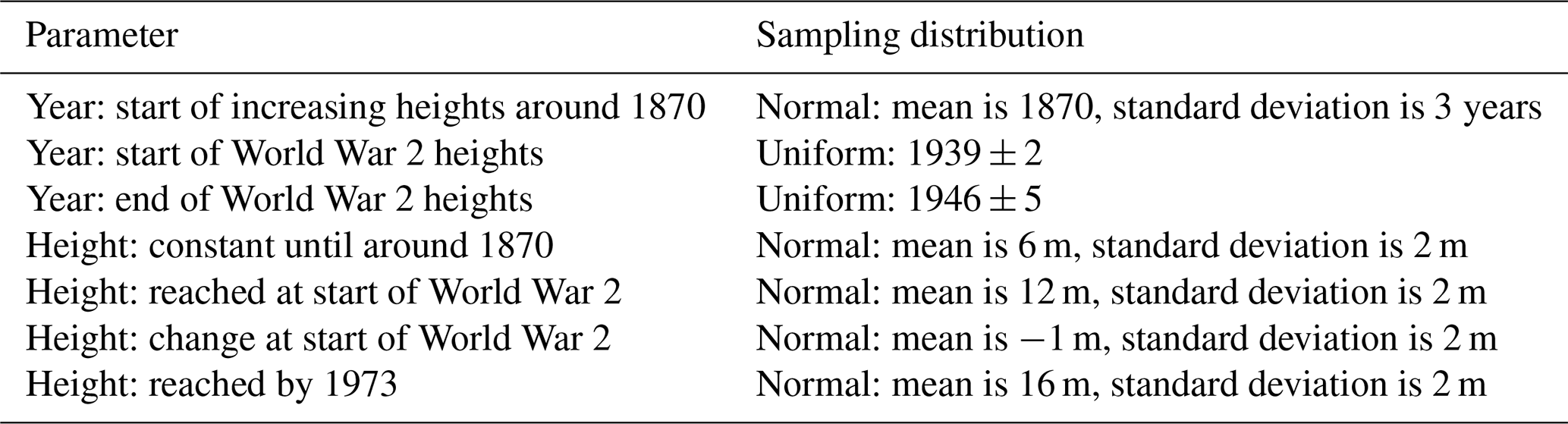
Prior to height information being available for individual observations from WMO Publication 47 (mostly pre-1973, before call signs were available to assign WMO Publication 47 entries to ships in ICOADS), observation heights are estimated from the literature following Kent et al. (2013). A 200-member ensemble is created to reflect uncertainty in measurement heights; the parameters for the ensemble are shown in Table 4. Per ship, the ensemble varies the height four times to reflect the change in average ship height over time (parameter prefix “height” in Table 4). The exact timing of the start of the height changes also forms a component of the ensemble to reflect uncertainty in that date (parameter prefix “year” in Table 4).

Table 4 Parameters used to construct the GloSATMAT height ensemble.

From 1970 onwards, the height of a ship is determined by joining the ICOADS ID (the ship call sign or other identifier) with the corresponding WMO Publication 47 entry. Sometimes, the height of the dry-bulb thermometer above the summer load line, i.e. the thermometer height, is used. However, if the thermometer height is missing then the height of the barometer, the anemometer, or the height of the visual observing height is used. If the height of the ship's thermometer (inferred from WMO Publication 47) is known, the assumed uncertainty in that height is ±1 m.

For missing heights after 1970, the height is sampled from the distribution of known heights from WMO Publication 47. Height information is grouped by 5° grid box, 10° grid box, country of registration, oceanic basin, 10° latitude band, vessel length, and vessel type. For IDs without a height, the height is sampled across a selection of heights where a ship has matching information. Observations without ship ID information are assigned a pseudo-ID and placed in a sub-group for which an ensemble of possible heights is generated. The overall estimated thermometer height for ships in ICOADS is shown in Fig. 2 of Cornes et al. (2020a).

To adjust MAT measurements to a standard reference height and quantify uncertainty in adjustments, we implement an ensemble version of the height adjustment method described in Cornes et al. (2020a). For each ensemble member, a single random sample of stability parameters (temperature scaling parameter and Monin–Obukov length, Biri et al., 2023) is taken in each 5° grid cell and 10 d period from a pool of 10 000 parameter sets, which comprises 5000 samples taken from the distribution of random uncertainty components and 5000 taken from the systematic components (see Cornes et al., 2020a). A fixed sample over each 10 d period within a month is used. This is designed to replicate the expected constancy of stability parameters within the synoptic timescale. For each sample of stability parameters and height estimates, the temperature data were adjusted to a height of 2 m above sea level.

2.2.3 Adjustment of observations during World War 2

The adjustment of data from ICOADS Decks 245 (UK Royal Navy Ships) and 195 (US Navy Ship Logs) during the period 1942–1945 follows the method described in Cornes et al. (2020a) to calibrate observations from these decks in relation to those in other decks. For GloSATMAT, the adjustments and uncertainty values have been calculated for both daytime and nighttime data. While the uncertainty in these adjustments was previously considered to be entirely correlated by ship track, the World War 2 adjustments have been partitioned so that one-third of the total uncertainty is modelled as correlated by ship track, while two-thirds of the uncertainty is uncorrelated. This partitioning addresses a problem with the error covariance matrices, which would otherwise not always have been positively semi-definite and hence could not have been used in further calculations.

2.2.4 Diurnal-heating bias adjustment

The Cropper et al. (2023) implementation of the Berry et al. (2004) heating bias model was used to quantify the expected diurnal influence on the MAT of energy storage and release by ship superstructures. On an annual basis, we fit a set of heating bias model coefficients to every uniquely identifiable ship track used from ICOADS following processing to improve the association of ship identifiers with individual ships as described in Cornes et al. (2020a). In addition, some ship IDs prior to 1850 were not unique and were assigned new unique IDs using additional information contained within the ship report. Where this was possible, the data for these problematic IDs were retained; otherwise, the data were excluded. The estimates of the heating bias are based on the difference from MAT and the underlying trend in nighttime temperature, defined as the temperature between 1 h after sunset until 1 h after sunrise. Hence, each MAT observation is adjusted by the difference between the estimated bias and the nighttime mean MAT. As such, the full diurnal cycle is removed from the data, and GloSATMAT should be considered to be a nighttime-equivalent data set.

As described in Cropper et al. (2023), 2500 alternate sets of heating bias model coefficients are determined from the full suite of ICOADS ships from the period of 1856–2020. For each individual ship, 2500 realizations of the heating model coefficients are generated, and an ensemble of 60 of these, minimizing several different cost functions, are selected as the best fit for each ship. The ensemble means of the adjustments over the 60 different ensemble members become the heating bias adjustment.

The data requirements for each observation to apply the heating bias adjustment are position, time, cloud cover, and relative wind speed. For a ship track to be included, we require at least 12 observations where the underlying nighttime MAT can be determined. If a ship track has partially missing cloud and/or wind speed values, these values are sampled from the 1961–1990 climatological distribution of cloud and wind derived from ICOADS after the 60 best model coefficient combinations have been selected. If a ship track has completely missing cloud and/or wind, the sampling occurs during the selection of the heating bias model coefficients.

Almost all observations pre-1856 lack cloud cover data, and many ships do not meet the criterion of having 12 observations for which the underlying nighttime MAT can be determined. In this period, we relax this requirement so that all observations in this period that pass QC can be included. For many ships, this means that the coefficients for the heating bias model cannot be fitted as there is no target nighttime information. In this situation, we use an ensemble of heating bias model coefficients computed from ships that do have the required data, whereby it is likely that these ships are typical during this period. The correlated uncertainty for MAT from ships fit this way is fixed at 0.45 °C, the 97.5th quantile over the 1857–1870 period.

2.3 The GloSAT GSAT reference analysis

2.3.1 LSAT anomaly grids

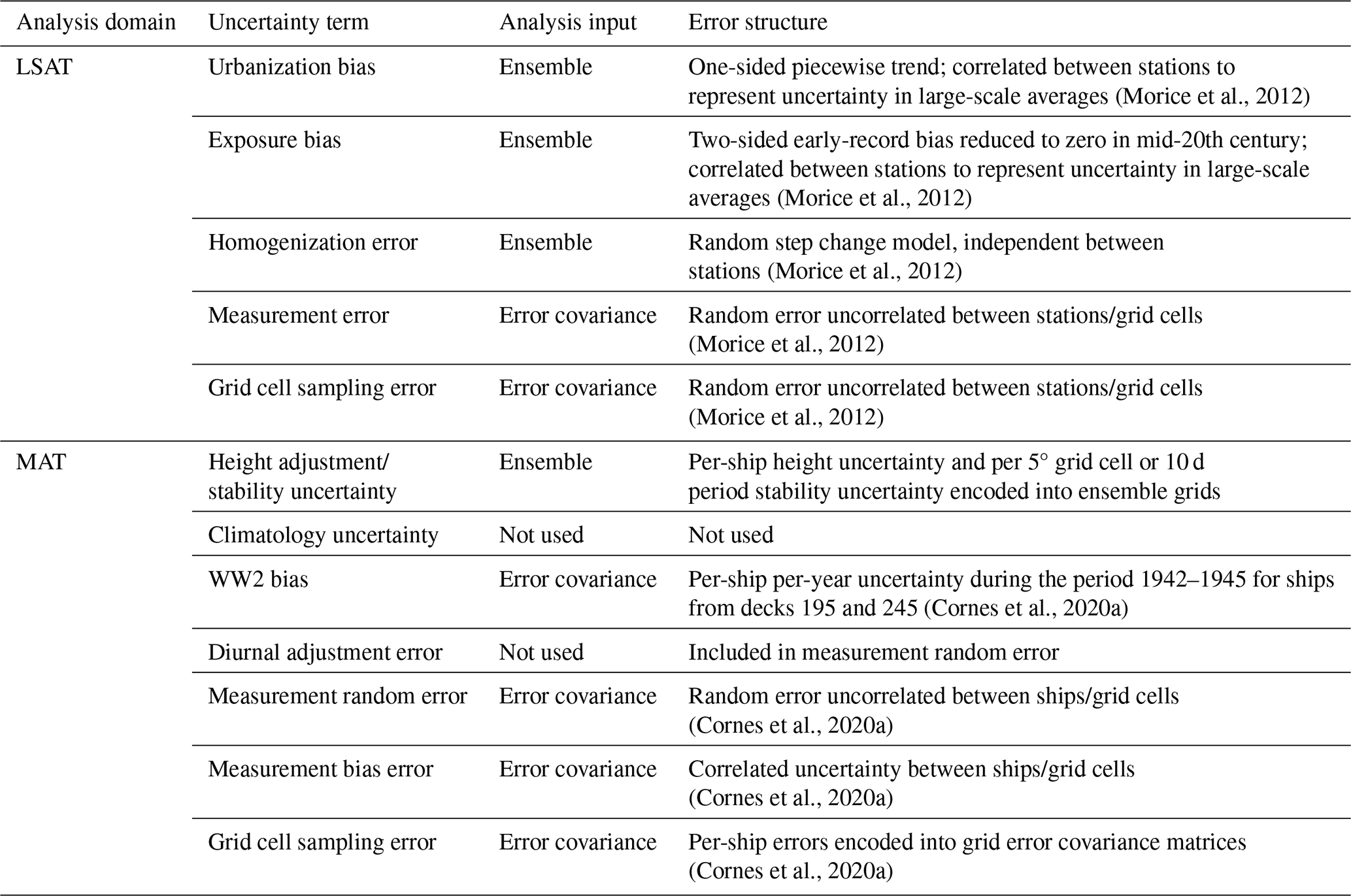
A 200-member ensemble of gridded LSAT fields has been constructed from station temperature series by applying the ensemble gridding procedure described in Morice et al. (2012). This includes ensemble sampling for homogenization uncertainty, exposure bias uncertainty, station climatology uncertainty, and urbanization uncertainty, which are accompanied by analytical estimates of measurement and sampling uncertainties, as in Morice et al. (2012). The exposure bias uncertainty model of Morice et al. (2012) is retained despite the addition of new exposure bias adjustments as the Wallis et al. (2024) adjustments are available for a subset of stations located at mid-latitudes only, and the adjustments are uncertain. The HadCRUT5 climatology uncertainty model is retained (Morice et al., 2012), with the HadCRUT5 uncertainty model for interpolated normals being used for LEK normals (Taylor et al., 2025). For these interpolated normals, the station climatology uncertainty σ_clim(m) for the calendar month m is a function of the standard deviation of monthly temperatures for the calendar month σ_var(m), with ${\mathit{\sigma }}_{\text{clim}}\left(m\right)={\mathit{\sigma }}_{\text{var}}\left(m\right)/\sqrt{\mathrm{15}}$. The resulting uncertainty is equivalent to that for a station with 15 years of available monthly averages within the climatology period.

Table 5 shows the mapping of uncertainty sources to the uncertainty model's ensemble members and error covariance matrices. These ensemble members and error covariance matrices form the inputs for a non-interpolated merged analysis and the resulting 200-member LSAT anomaly ensemble grids are then used as inputs into the Gaussian-process-based infilling method described in Morice et al. (2021) and previously used to create the HadCRUT5 data set (see Sect. 2.3.3).

(Morice et al., 2012)(Morice et al., 2012)(Morice et al., 2012)(Morice et al., 2012)(Morice et al., 2012)(Cornes et al., 2020a)(Cornes et al., 2020a)(Cornes et al., 2020a)(Cornes et al., 2020a)

Table 5 Representation of uncertainty model components in LSAT and MAT error models.

2.3.2 MAT anomaly grids

A 200-member marine air temperature ensemble has been generated based on the 200-member ensemble of diurnally adjusted all-hour marine air temperature observations adjusted to a 2 m reference height. Each ensemble member is gridded separately following the method described in Cornes et al. (2020a) using the ship observation ensembles that sample uncertainty in height adjustments and World War 2 (WW2) adjustments. As in CLASSnmat v1, these gridded fields are initially generated as monthly actual MAT values, and then climatological averages are subtracted from the gridded data to produce the anomaly fields. Missing values in the GloSATMAT climatology fields are filled using a thin-plate spline with the smoothing parameter set to zero. In this way, the spline acts as an exact interpolator, and, hence, where grid cell values exist, these are reproduced exactly in the interpolated field. Missing cells are interpolated from non-missing cells in the neighbourhood, and this allows anomaly values to be calculated in regions where there are insufficient values over the climatological period to construct a 30-year mean value. The gridded anomaly values are calculated by subtracting this climatology from the gridded actual temperature fields for the respective month of the year. As a final QC check on the gridded data, any grid cell MAT anomalies greater than 10 °C or less than −10 °C are removed. It should be noted that these climatologies differ slightly from the values used in the earlier climatological QC (see Sect. 2.2.1).

Following the example of the CLASSnmat data set, uncorrelated, systematic, and sampling uncertainties are encoded into monthly error covariance matrices, excluding terms included in the ensemble. Uncertainty in diurnal-heating adjustments is encoded into these error covariance matrices and treated as uncorrelated between observations. A summary of uncertainty model components is provided in Table 5. The 200-member gridded MAT ensemble and accompanying error covariance matrices are provided as inputs into the Gaussian-process-based infilling method (previously used to create the HadCRUT5 data set, Morice et al., 2021) to generate a 200-member infilled MAT anomaly ensemble.

2.3.3 LSAT and MAT interpolated analyses

Interpolated analyses of LSAT and MAT are produced using the Gaussian process analysis system of Morice et al. (2012). This analysis method takes ensemble gridded temperature anomaly fields as inputs, modelling systematic error structures in observed air temperature anomalies. An additional observational error structure is provided to the analysis in error covariance matrices. The full details of the method are provided in Morice et al. (2021).

Separate LSAT and MAT analyses are produced. Ensemble and error covariance inputs into the analysis equations are summarized in Table 5. The LSAT analysis error model structure matches that used in the HadCRUT5 data set, with the structure of individual uncertainty components described in Morice et al. (2021). For the MAT analysis, the encoding of error structures into the input 200-member MAT ensemble grids and the accompanying error covariance matrices is described in Sect.  2.2 and in Cornes et al. (2020a) and Cropper et al. (2023).

Analysis estimation follows the method of Morice et al. (2021) using the HadCRUT5 analysis processing system. As in Morice et al. (2021), the Gaussian process models monthly temperature anomaly fields as the sum of a monthly field mean and a spatially varying Gaussian process. The Gaussian process model uses a Matérn covariance function that models covariances between locations on the Earth's surface as a function of Euclidian distance. As for HadCRUT5, the Matérn covariance function's smoothing parameter is set to η=1.5. Parameters representing the standard deviation of temperature anomaly variability σ and spatial decorrelation length scales ρ are estimated separately for land and ocean analyses as the average of maximum likelihood estimates for monthly fields from 1961 to 1990. The resulting parameter estimates for the LSAT analysis are σ=1.2 °C and ρ=1300 km, and those for the MAT analysis are σ=0.65 °C and ρ=1550 km. For comparison, these LSAT parameter estimates for GloSATref are the same as for HadCRUT5, but the GloSATref MAT parameter estimates differ from those for SST in HadCRUT5, which have a lower amplitude (σ=0.6 °C) and shorter length scale (ρ=1300 km).

As in the HadCRUT5 data set, the analyses are masked in regions of weak observational constraint, defined by a metric of 1 minus the ratio of the posterior to prior variance of the spatial model estimates at each analysis grid cell. The analysis is masked where this metric takes a value of less than α=0.25 (see Morice et al., 2021, and their supporting information for discussion).

2.3.4 Merging LSAT and MAT analyses

The GSAT ensemble grids are produced as weighted averages of MAT and LSAT anomaly ensemble grids. The weighting scheme follows the HadCRUT5 method, with weighting based on the fraction of land area in each grid cell. As in HadCRUT5, for the interpolated analysis, sea ice regions are treated as if they were land in the weighting scheme, and a minimum weighting of 25 % land is placed on grid cells that are directly observed by land meteorological stations. These choices are retained from HadCRUT5 to aid comparison of the climate diagnostics based on SST and MAT through comparison of HadCRUT5 and the GloSAT reference analysis.

3 Results and discussion

3.1 Global and hemispheric temperature anomaly series

Figure 1 shows a comparison between GloSATref and HadCRUT5 interpolated global and hemispheric analyses, including uncertainty ranges and percentages of global and hemispheric coverage. Each of these two analyses is produced using the HadCRUT5 analysis methodology. Differences in global annual average time series between these two analyses reflect the differences in input LSAT and MAT and/or SST data sets and their uncertainties combined with the interaction between anomaly patterns and data coverage in those input data sets and the spatial interpolation methods.

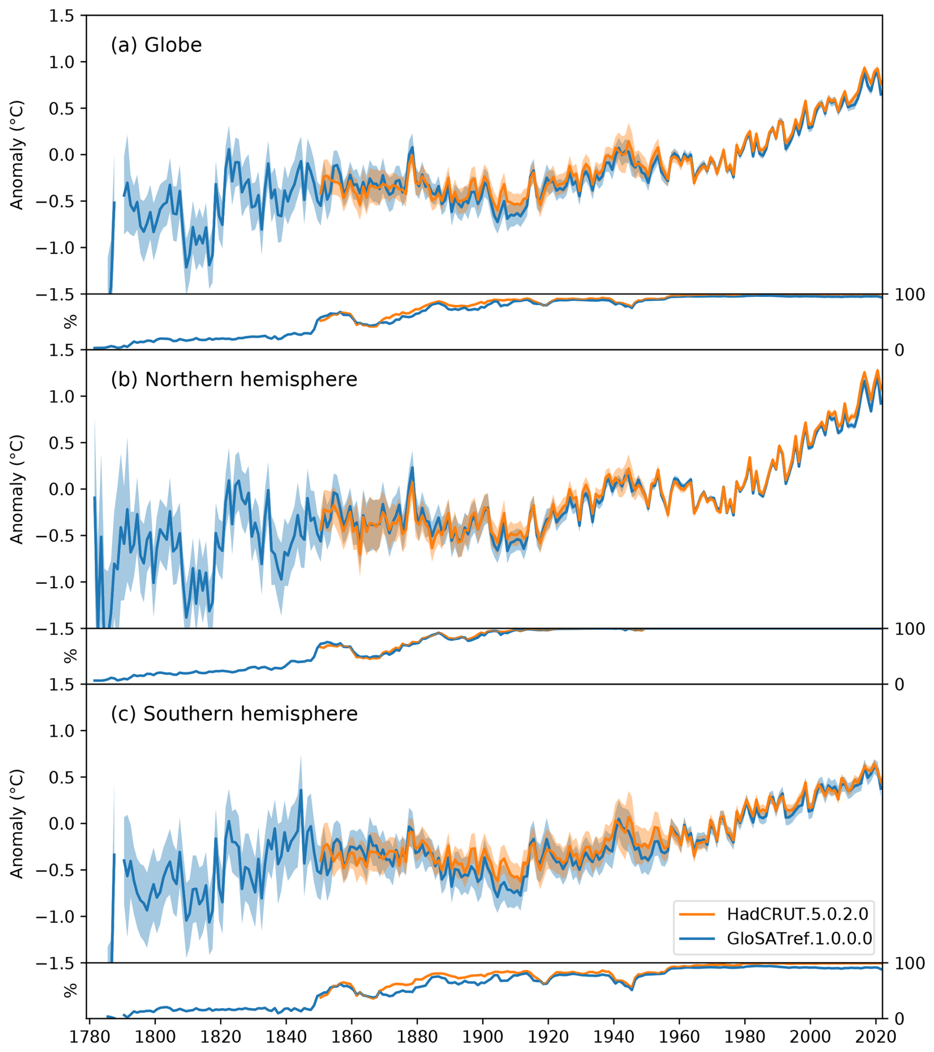
Figure 1 Global and hemispheric average temperature anomaly time series for the GloSATref and HadCRUT5 global analyses (°C, relative to 1961–1990), together with the percentage of areal grid coverage for (a) the full globe, (b) the Northern Hemisphere, and (c) the Southern Hemisphere. Hemispheric series omit years in which there are no data available in the respective hemisphere. Global averages are computed as an average of northern- and southern-hemispheric series, requiring data to be available in both hemispheres. Methods for computation of time series and their uncertainties are provided in Morice et al. (2021).

GloSATref, like HadCRUT5, represents the major changes we expect to see in the global mean. The pre-1850 record, despite its increased uncertainty, captures the strong cooling associated with major volcanic eruptions. The overall warming of global temperature is clear, although GloSATref warms slightly less overall. Features noted in previous comparisons of SST and NMAT large-scale averages remain prominent in the GloSATref comparison to HadCRUT5, for example, the lower temperatures in the early 1900s and in recent years (Cornes et al., 2020a; Gulev et al., 2021; Chan et al., 2024).

For their period of overlap, currently 1850 to 2021, there is broad agreement in the global and hemispheric means. While areal coverage of the Northern Hemisphere is similar in the two data sets, GloSATref has slightly reduced southern-hemispheric coverage compared to HadCRUT5. GloSATref is, on average, warmer than HadCRUT5 from the start of the latter data set in 1850 until 1880 and then more notably cooler, on average, than HadCRUT5 until the early 1910s, especially in the Southern Hemisphere.

Variability in GSAT and hemispheric averages from GloSATref is high in the period before the start of HadCRUT5 in 1850, as expected from the lower data coverage. There are two periods of strong cold anomalies which result from the cooling of the atmosphere following the eruptions of major volcanos: Laki in 1783–1784 (Zambri et al., 2019), an eruption of unknown source in 1808, Tambora in 1815, and further eruptions in the 1820s and 1830s (Brönnimann et al., 2019). It is likely that the global mean effect of Laki is overestimated in this time series (Fig. 1a) because it is influenced by the location of the available observations in the 1780s; this effect can be seen in model simulations masked in relation to the GloSATref data coverage (Ballinger et al., 2025).

3.2 Temperature anomaly maps and data coverage

The most obvious feature in the 20-year averages of SAT anomalies shown in Fig. 2 is the increase in temperature over time, particularly at high northern latitudes. The period before about 1820 is particularly cold, likely due to volcanic activity. Warm anomalies are present in higher latitudes of the North Atlantic in the 20-year averages from 1821–1840 to 1881–1900 and the of the South Atlantic from 1821–1840 to 1861–1880. These might be indicative of multidecadal variability. The Arctic region is relatively warm in the 1920s and 1930s (Hegerl et al., 2018). Despite the new adjustments to MAT for biases present during WW2, this period may still be unrealistically warm in GloSATref according to a new analysis of SST data (Chan et al., 2024).

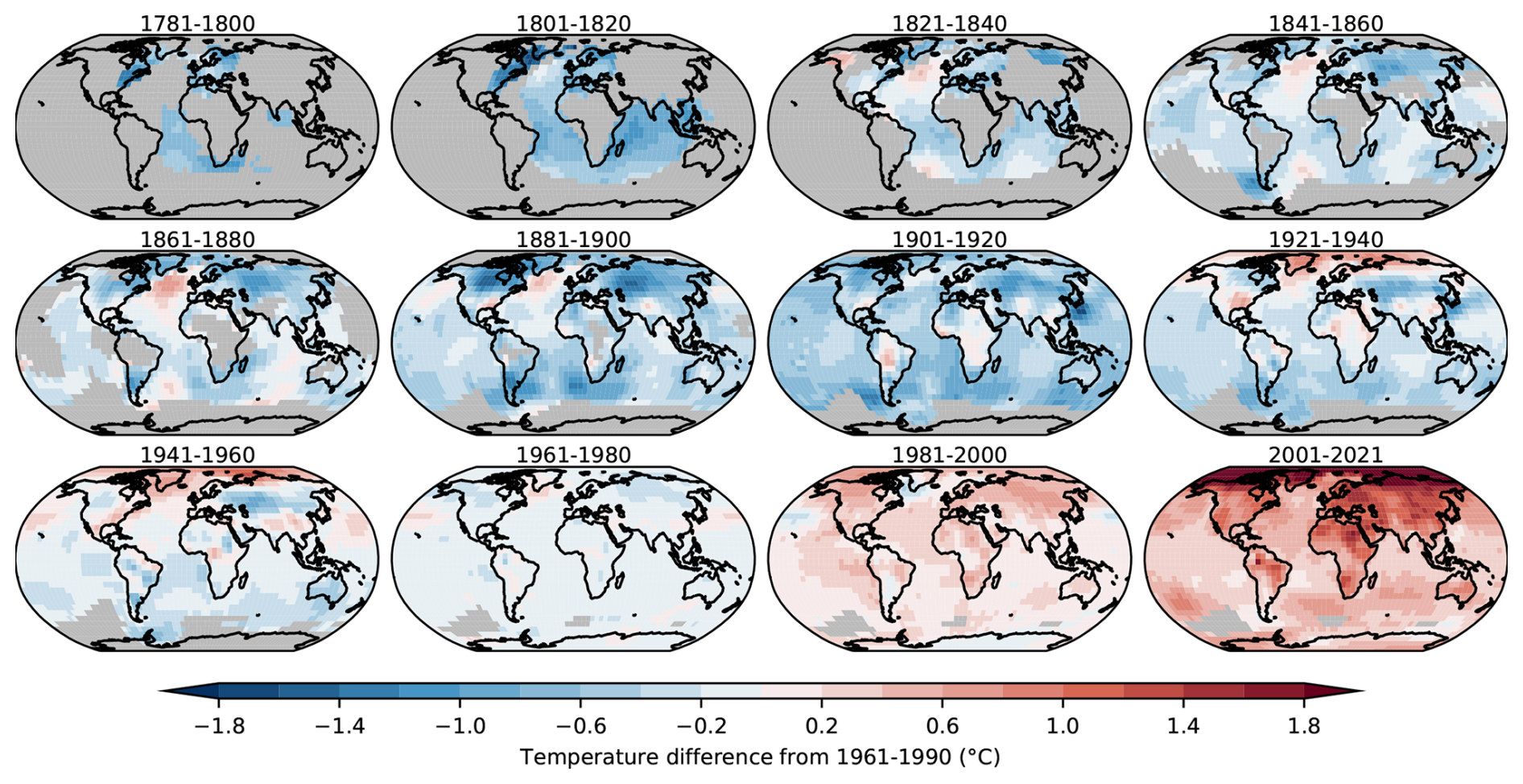
Figure 2 The 20-year average SAT for the GloSATref analysis (°C relative to 1961–1990; final panel shows 21-year average). Each panel averages available gridded data to quarterly, annual, and then 20-year (21-year) averages, requiring data in at least two quarters to form an annual average and at least 10 annual averages to produce a 20-year average.

While the use of MAT allows GloSATref to extend prior to 1850, there is nevertheless a marked reduction in data availability prior to about 1855 (see global coverage metrics in Fig. 1 and 20-yearly coverage maps in Figs. S1 and S3 in the Supplement). Before 1850, the majority of weather station LSAT series are situated in Europe and the eastern coast of North America, limiting Northern Hemisphere coverage of the GloSATref analysis fields. Combined with an absence of station records in the Southern Hemisphere, this contributes to increased uncertainty in global and hemispheric series. MAT coverage is predominantly restricted to the Atlantic and Indian oceans, reflecting primary trade routes. For these regions it is possible to make estimates of regional temperature anomalies based on GloSATref analysis fields using reasonable criteria for data availability (Fig. 2). The Pacific has highly limited sampling in this early period. Non-uniform global coverage in the early record may lead to a sampling bias in global average SAT estimates in this period. Uncertainties in global and hemispheric means are therefore larger in this early period as both LSAT and MAT are sparsely observed, but the uncertainty estimates themselves are likely to be less robustly quantified.

Observation coverage improves over time, accompanied by increased global coverage of the gridded analysis fields. In the second half of the 1800s, there is a marked increase in station LSAT series availability, with analysis estimates becoming available by the end of the century for most land regions excluding Antarctica; interior regions of Africa; and northern regions of South America, including the Amazon. By the 1880s, measurements from all oceans are available, although with varying degrees of data availability. While sufficient data are available to estimate average temperature anomalies across much of the Pacific at this time (Fig. 2), data coverage in the analysis is limited in regions of the western and southern Pacific. Data coverage for the Southern Ocean and high northern latitudes is highly limited.

In the early 20th century, most of the missing grid cells are in the Southern Ocean and over Antarctica. Underpinning land station data coverage remains limited for much of Africa, South America, interior regions of eastern Asia, and high-latitude regions of North America and Eurasia, although the available observation coverage permits analysis estimates for these regions. The Antarctic becomes represented in the analysis in the 1950s. Coverage for MAT peaks in the 1970s and 1980s and has declined markedly since (Berry and Kent, 2016; Kent and Kennedy, 2021). Observation coverage of the Southern Ocean and the southern extents of the Pacific, Atlantic, and Indian oceans remains reduced in GloSATref in comparison to HadCRUT5 in recent decades (see Figs. S1–S4). SST observations from drifting buoys contribute notably to differences in marine data coverage in these regions, but there are also fewer ship observations of MAT than of SST.

As in the preceding CRUTEM5 station database (see discussion in Osborn et al., 2021), the number of LSAT series is relatively high and stable from the early 1960s to the early 2010s, with a sharp reduction in the last decade due in part to delays in accessing data. However, in CRUTEM5, the number of station series actually used in the gridding showed a decline from the 1970s onwards, falling to below 90 % of its 1970s peak from 1991 onwards (Fig. 7 of Osborn et al., 2021), and this is mostly because new stations installed from the 1970s onwards did not have the data necessary to estimate their 1961–1990 normals. In the current study, the use of Kriging (Sect. 2.1.3) to estimate missing values from neighbouring stations for the purpose of estimating normals has partly ameliorated this issue: the number of stations used for gridding is 90 % of its 1970s peak as late as 2011 (compared with 1991 in CRUTEM5). It is worth noting, though, that these additional stations that can now be used for the gridded data set are commonly in grid cells with other LSAT stations; therefore, their importance is that they reduce the sampling uncertainty at the grid cell level rather than extending coverage of the gridded data set in the final decades.

Differences in temperature anomalies over land between HadCRUT5 and GloSATref (Fig. 3) result from the increased number of stations used to create the GloSATref grids, primarily from use of the LEK method and from early-record mid-latitude screen bias adjustments. The effects of screen bias adjustments are evident in anomaly difference maps prior to the 1930s, most notably with HadCRUT5 containing warmer anomalies across Eurasia in the 1890–1909 and 1910–1929 panels and in western North America in the 1850–1869 panel. This difference is largest in the summer and autumn months when Northern Hemisphere screen biases are largest, for which HadCRUT5 does not include adjustments. From the 1930s onwards, differences between HadCRUT5 and GloSATref anomalies over land are minimal.

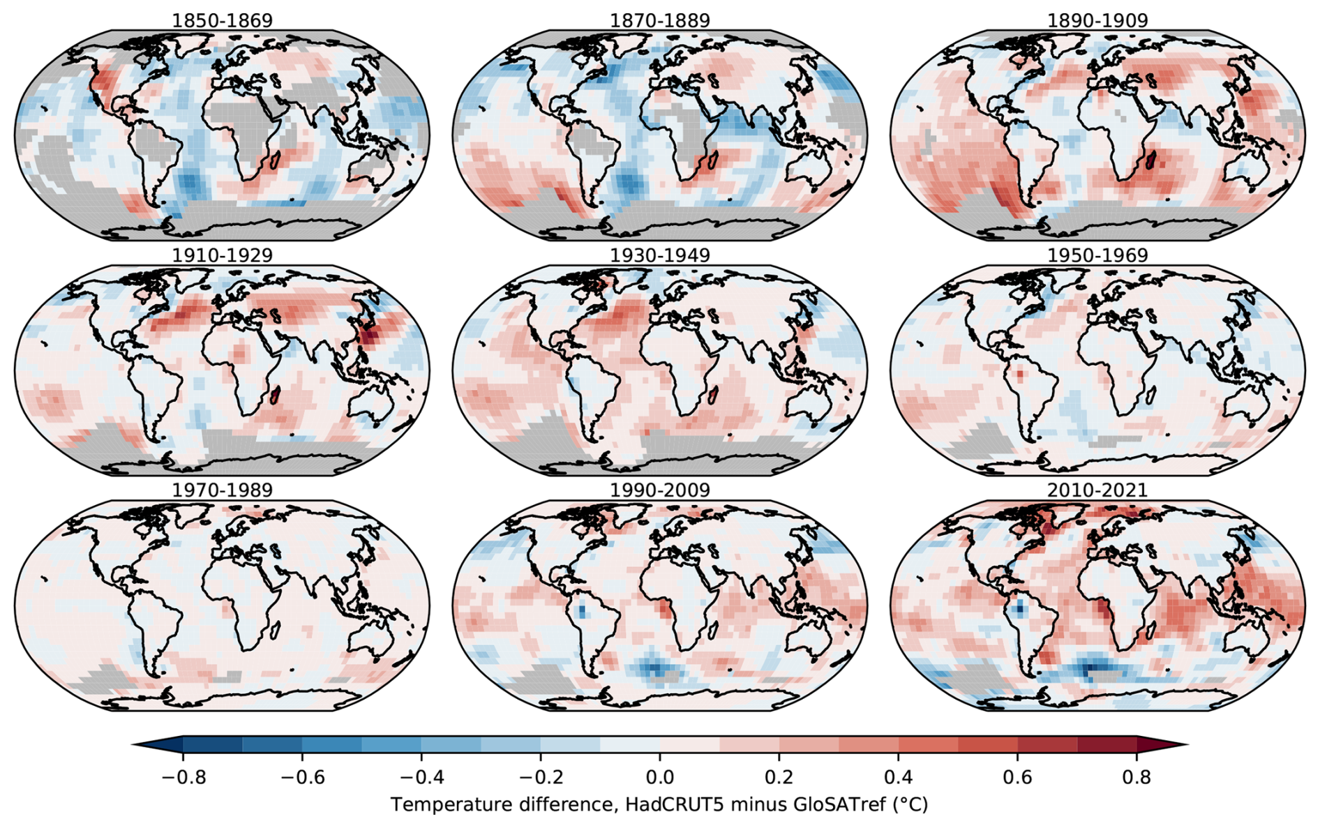
Figure 3 Difference in 20-year average anomalies, relative to 1961–1990, between the HadCRUT5 and GloSATref analyses (°C; final panel shows 12-year average). Blue colours indicate where HadCRUT5 is colder than GloSATref. Red indicates where HadCRUT5 is warmer.

3.3 Effects of MAT and LSAT updates in global series

Global average anomaly time series for GloSATref, GloSATLAT, and GloSATMAT are shown in Fig. 4 in comparison to methodologically related data sets, showing the effects of data and methodological changes contributing to GloSATref. Additional land and marine data set comparisons are shown in Figs. S7 and S8, including a broader range of data sets.

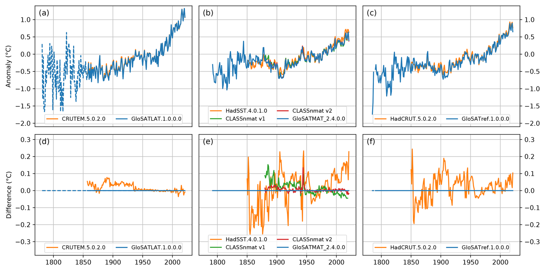
Figure 4 Top row (a–c): global average temperature anomalies (°C) relative to 1961–1990 for (a) LSAT; (b) SST, NMAT, and/or MAT; and (c) GMST and/or GSAT. Bottom row (d–f): differences in global average 1961–1990 temperature anomaly time series for (d) LSAT minus CRUTEM.5.0.2.0 LSAT; (e) SST, NMAT, and/or MAT minus HadSST.4.0.1.0 SST; and (f) GMST and/or GSAT minus HadCRUT.5.0.2.0. The dashed line for GloSATLAT extends the series prior to 1856 by omitting the requirement for at least five populated grid cells in each hemisphere, with only Northern Hemisphere station data present in GloSATLAT grids prior 1854. None of the LSAT, SST, NMAT, and/or MAT data sets in panels (a, b, d, e) use spatial interpolation, while spatial interpolation is used in GSAT and/or GMST analyses shown in panels (c, f). Plotted series use all available gridded data without co-location to common data coverage.

Averaging globally over the land domain for the non-interpolated GloSATLAT data (noting that coverage becomes increasingly limited during the first 100 years) and comparing to the closely related CRUTEM5 data set (Fig. 4a and d) show that the Wallis et al. (2024) exposure bias adjustments cool LSAT global annual averages in the 19th and early 20th centuries by less than 0.1 °C, primarily through mitigation of summer warm biases, which are larger than the annual bias adjustments. Differences from CRUTEM5 in the 21st century are less than 0.04 °C of either sign. These differences result from the expanded set of station records included in anomaly grids.

Comparing the all-hour GloSATMAT to related NMAT data sets, CLASSnmat v2 uses the same methodology and input data sources as GloSATMAT but, like its predecessor CLASSnmat v1, excludes daytime observations and starts in 1880. The main reason for the differences between the two versions of CLASSnmat is the addition of extra data sources (see Sect. 2.2.1 and Fig. 4b and e). CLASSnmat v2 is therefore most similar to GloSATMAT. For most of the period of 1850–1879, where there are only estimates from GloSATMAT and HadSST4, GloSATMAT is warmer than HadSST4 on average by about 0.1 °C, which may suggest either an incomplete removal of diurnal-heating biases in GloSATMAT or a residual cold bias in HadSST4. This relative warmth compared to HadSST4 is also seen for the first decade of the NMAT records. The early 20th century shows rapid variations in the difference between the MAT data sets and HadSST4. Recent analysis has suggested that most SST data products, including HadSST4, may be biased cold during the early 20th century (Sippel et al., 2024; Chan et al., 2024); further work is required to understand the different temperature records in this period. During WW2, GloSATMAT shows cold temperature anomalies relative to both HadSST4 and the NMAT-based estimates. This may suggest that the new bias adjustments are an improvement (Sect. 2.2.3) as a new analysis by Chan et al. (2024) indicates that HadSST4 may contain residual warm biases during WW2.

The smaller warming trend in NMAT relative to SST data has been noted for some time (for an overview, see Cornes et al., 2021; Gulev et al., 2021). This feature is also apparent in the MAT data presented here (Fig. 4) and is shown to start in the late 1950s. SST and air temperature anomaly differences in this period are larger in tropical regions but are more similar during El Niño periods (not shown). Climate models and atmospheric reanalyses show the opposite relationship between SST and MAT trends (Gulev et al., 2021), supported by a proposed physical constraint (Richardson, 2023). Further analysis of the in situ marine observations is therefore required.

Global average temperature series for GloSATref and HadCRUT5 analyses are shown in Fig. 4c (as in Fig. 1 but without the uncertainty range), and their differences are shown in Fig. 4f. Over their common period, comparison with averages derived from their underpinning single-domain data sets indicates that differences in terms of the time variation of global temperature anomaly series for GloSATref and HadCRUT5 primarily arise from their marine components, with early-record LSAT exposure bias adjustments having a smaller effect.

3.4 Comparison to other GMST data sets

The global average temperature time series for the GloSAT GSAT analysis is shown in Fig. 5 alongside those of current GMST analyses. Figure 5b gives a more detailed view of their differences from GloSATref. As noted in Sect. 1, the GMST data sets differ in terms of the methods used and the underpinning observation data, although there are overlaps and commonalities between them in both respects.

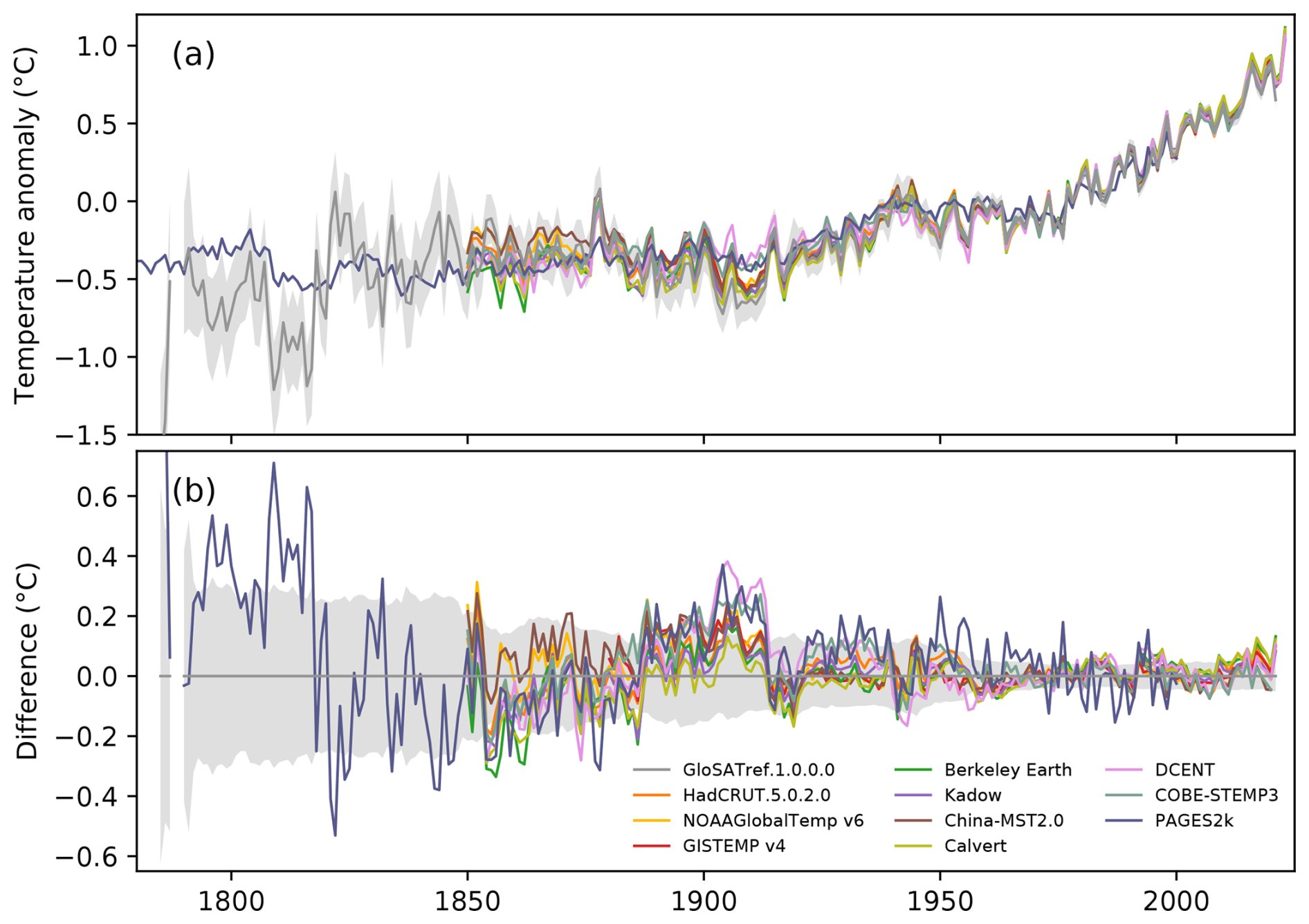
Figure 5 (a) GSAT and GMST (°C, relative to 1961–1990) derived from instrumental data sets and the ensemble median of the PAGES2k palaeoclimate reconstructions and (b) differences between GloSATref and instrumental GMST and the PAGES2k ensemble median (each series minus GloSATref). Solid lines show the ensemble means or medians where the data set provides an ensemble; grey shading is the 2.5 % to 97.5 % confidence interval for the GloSATref series only. All instrumental series are January–December annual averages. PAGES2k series are representative of April–March annual averages.

Also shown is the global average temperature anomaly time series for the median of the PAGES2k multi-proxy ensemble reconstructions (PAGES2k, 2019). The PAGES2k ensemble was calibrated using the Cowtan and Way (2014) spatially infilled analysis of HadCRUT4 data over 1850–2000 so that (by weighting and scaling the proxy records) it resembles the overall warming and some of the variability of the infilled HadCRUT4. The pre-1850 period is not directly constrained in this way, and it is for comparison with GloSATref during this period that it has been included.

There is general agreement between all of the estimates, with particularly good agreement regarding the representation of interannual variability among the instrumental-based data sets. From 1850 to around 1885, there is a wider scatter between the various data sets, with some warmer and some cooler than GloSATref, reflecting the greater uncertainty in these early observational data sets. This is also a period when these other data sets lie outside the GloSATref 95 % confidence range more often.

From 1888 to 1913, GloSATref is consistently cooler than the SST-based data sets, and, at times, they all lie outside the GloSATref 95 % confidence range during this period, except for the HadCRUT5-based Calvert (2024) data set. This difference is notable because there is evidence that this early-20th-century cool period is biased cold in the SST data sets (Sippel et al., 2024), yet GloSATref is cooler still by 0.1 to 0.2 °C. The SST-based data sets are more similar to each other than to GloSATref due to differences between SST and MAT (see Fig. 4e). Differences over 1888 to 1913 (Fig. 5) are most prominent for the DCENT and COBE-STEMP3 data sets (Chan et al., 2024; Ishii et al., 2025), with each being notably warmer than GloSATref over 1888 to 1913 and exhibiting excursions beyond the GloSATref 95 % confidence intervals throughout the first half of the 20th century. These two recently published data sets have new treatments of inhomogeneities. Each uses land station LAT values in their respective SST bias adjustment schemes. While the specifics of their adjustment methods differ, each method acts to reduce differences between detrended global average SST and LSAT anomalies. These two data sets also add SST data-source-based adjustments that impact early-20th-century warming: COBE-STEMP3 includes an adjustment to address a truncation error in a prominent underpinning data source in this period, the KOBE collection (Chan et al., 2019), while DCENT uses an SST adjustment scheme based on nation, ICOADS deck, and measurement method (Chan and Huybers, 2021). The PAGES2k ensemble median palaeoclimate reconstruction (PAGES2k, 2019) is warmer than GloSATref and much closer to DCENT and COBE-STEMP3 during this early-20th-century period.

From the 1930s to the end of the 20th century, differences between GloSATref and GMST data sets based on ERSST v5 (GISTEMP and NOAAGlobalTemp) are, on average, smaller than differences with HadSST4-based data sets (HadCRUT5 and Berkeley Earth). This is likely to be related to the more direct use of NMAT observations to bias adjust ERSST v5 SSTs rather than HadSST4 SSTs. Similar results may be expected once data sets based on ERSST v5 are updated to use the recently published ERSST v6 (Huang et al., 2025a, b). From the 1950s onwards, the dominant difference is the slightly lower trend in MAT relative to SST, as noted earlier. This leads to GMST data sets lying above the GloSATref confidence range in recent years.

Before 1850, the only comparison is with data from the palaeoclimate record. During this period, GloSATref shows much greater variability than it does after 1850 (arising especially from the land component: Fig. 4) and much greater variability than the PAGES2k median global temperature reconstruction (Fig. 5a), with the PAGES2k median extending outside both the 2.5 % and 97.5 % confidence limits of GloSATref at times (Figs. 5b and S6). There is a possible step in the PAGES2k-GloSATref difference around 1820 (Fig. 5b), but this is the type of feature that occurs when differencing a highly variable series with a smoother lower-variance series, and so it is not strong evidence for a discontinuity in either GloSATref or PAGES2k. There are multiple reasons for the differences between GloSATref and PAGES2k prior to 1850. The variance of the PAGES2k median may be too small due to averaging over multiple possible realizations (PAGES2k ensemble range is not shown here but is shown in Fig. S6) as discussed by PAGES2k (2019) and Anchukaitis and Smerdon (2022). It is likely that pre-1850 variability in the GloSATref global series is overestimated by much reduced global measurement sampling (Fig. 2), which increases uncertainty and variance in the global mean estimate. This is especially the case for the land data, which are limited almost entirely to Europe before 1820. Coverage uncertainty estimates for the GloSAT series (based on sub-sampling late-20th-century and early-21st-century ERA5 reanalysis fields in relation to the observed locations) are, indeed, larger during this period but may not fully represent this uncertainty. The underlying measurements in the early 19th century were taken from less standardized instruments and measurement platforms and will likely have larger uncorrected errors, which contribute to increased variance. Part of the enhanced variability is likely to be due to strong volcanic activity, with the GloSATref series cooling around the times of the unidentified 1809 volcanic eruption and the 1815 eruption of Mount Tambora and, to a lesser degree, around the time of the 1830s eruptions. It is possible that this volcanic response is not fully captured in the PAGES2k median (Anchukaitis and Smerdon, 2022).

4 Data availability

The GloSATref analysis and its constituent data sets are available via the CEDA archive.

• The GloSATref analysis (Morice et al., 2025b) is available at https://doi.org/10.5285/a2519624a593402a83246bd359d098be.

• The GloSATLAT data set and station files (Morice et al., 2025a) are available at https://doi.org/10.5285/ef237f578329487eb02fb42f9db56bb2.

• The GloSATMAT data set (Cornes et al., 2025b) is available at https://doi.org/10.5285/e6251bf935304cfbb9c9269dc7757a35.

Data used in comparison plots

• Berkley Earth (Rohde et al., 2013a, b; Rohde and Hausfather, 2020): https://www.berkeleyearth.org (last access: 10 September 2024).

• Calvert (Calvert, 2024): https://doi.org/10.26050/WDCC/HadCRU_MLE_v1.2.

• COBE-STEMP3, COBE-LSAT3, COBE-LSAT3 (Ishii et al., 2025): https://climate.mri-jma.go.jp/pub/archives/Ishii-et-al_COBE-SST3 (last access: 21 May 2025).

• China-MST 2.0 – Imax (Sun and Li, 2021): https://doi.org/10.6084/m9.figshare.16929427.v4.

• CLASSnmat v1 (Cornes et al., 2020b): https://catalogue.ceda.ac.uk/uuid/5bbf48b128bd488dbb10a56111feb36a/.

• CLASSnmat v2 (Cornes et al., 2025a): https://doi.org/10.5285/306246329ae04eb3b2299446d911530a.

• CRUTEM.5.0.2.0 (Osborn et al., 2021): https://www.metoffice.gov.uk/hadobs/crutem5/ (last access: 10 January 2024).

• DCENT, DCSST, DCLAT v1.0 (Chan et al., 2024): https://doi.org/10.7910/DVN/NU4UGW.

• ERSST v6 (Huang et al., 2025a, b): https://www.ncei.noaa.gov/pub/data/cmb/ersst/v5/2023.ersst.v6 (last access: 2 May 2025).

• GISTEMP v4 (Lenssen et al., 2019): https://data.giss.nasa.gov/gistemp/ (last access: 10 September 2024).

• HadCRUT.5.0.2.0 (Morice et al., 2021): https://www.metoffice.gov.uk/hadobs/hadcrut5/ (last access: 10 January 2024).

• HadSST.4.0.1.0 (Kennedy et al., 2019): https://www.metoffice.gov.uk/hadobs/hadsst4/ (last access: 21 May 2024).

• Kadow version 6. (Meuer et al., 2024): https://doi.org/10.5281/zenodo.11262704.

• NOAAGlobalTemp v6 (Huang et al., 2024; Yin et al., 2024; Huang et al., 2022): https://doi.org/10.25921/rzxg-p717.

• PAGES2k (Neukom et al., 2019): https://doi.org/10.25921/tkxp-vn12.

• UAHNMATv1 (Junod and Christy, 2020): https://www.nsstc.uah.edu/users/robert.junod/UAHTEMP/UAHNMAT/UAHNMATv1_6190_ref.nc (last access: 21 May 2025).

5 Conclusions

A new global surface air temperature (GSAT) anomaly data set has been produced: GloSATref. This is the first such data set to use marine air temperature (MAT) instead of sea surface temperature (SST) in combination with land surface air temperature (LSAT). The use of MAT has allowed for the extension of the global measurement-based record back to 1784, with a land-only analysis back to 1781, adding nearly 70 years when compared to data sets using SST as their marine component and which start in 1850 or later. The construction of a MAT-based data set required overcoming several challenges, most notably the derivation and application of adjustments to account for warm biases due to daytime heating of the ship and sensor environment (Cropper et al., 2023). Similarly, for air temperature observations made over land, new estimates of bias were required to be able to use observations made before the widespread adoption of Stevenson-style screens to shelter the thermometers from the direct or indirect effect of solar radiation (Wallis et al., 2024). These adjustments will also improve the existing LSAT record (Osborn et al., 2021) before about 1930.

Extending the instrumental near-surface temperature record earlier in time by nearly 70 years gives an estimate of temperature changes associated with a period of strong volcanic activity between the 1780s and the 1820s, albeit requiring consideration of limitations in early global data coverage. These data are a new resource for the study of the climate of this early instrumental period (e.g. as in Ballinger et al., 2025) and provide an additional line of evidence for understanding global near-surface temperature change and variability alongside existing GMST data sets.

Instrumental monitoring of GSAT is contingent on sustained observation of air temperature over ocean and land. At present, the marine air temperature observing network is less robust than that for SST, with numbers of MAT observations having declined since the 1990s (Kent and Kennedy, 2021). Similarly, the LSAT record is dependent on maintenance of meteorological station networks and international data exchange. Support for international data infrastructure to meet the requirements of the construction of long-term climate records remains essential (Folland et al., 2001; Kent et al., 2019; Li et al., 2021). Equally important is support for data rescue through imaging and digitization of observations to improve global sampling and of metadata to improve our understanding of observing methods throughout the record (Brohan et al., 2009; Brönnimann et al., 2018; Luterbacher et al., 2024).

Global data sets based on SST have been produced for more than 30 years and have improved as our understanding of the characteristics of the observations has improved and as our methods of data set construction have advanced. Similar improvements can be expected with records based on MAT if resources permit. This new global surface air temperature analysis provides an additional line of evidence of changes in global temperature alongside existing GMST data sets and reanalyses.