Global spatially-distributed sectoral GDP map for disaster risk analysis

Global risk assessments of economic losses by natural disasters while considering various land uses is essential. However, sector-specific, high-resolution pixel-level economic data are not yet available globally to assess exposure to local disasters such as floods. In this study, we employed new land-use data to construct a global, spatially distributed map of sector-specific gross domestic product (GDP). We developed three global GDP maps, SectGDP30, in 2010, 2015, and 2020 for the service, industry, and agriculture sector with 30 arcsec resolution. The map (SectGDP30) demonstrates strong consistency (R² > 0.9) with actual sub-national statistical data, exhibiting superior alignment compared to conventional GDP maps (PB-method) reliant solely on gridded population information. The methodology refined GDP distribution for specific sectors. Industry GDP was more accurately mapped using non-residential land areas as a proxy, effectively capturing its localized concentrations. Agriculture GDP's accuracy improved by incorporating cropland data and a distance-based distribution assumption from population agglomeration. Application of this dataset in estimating flood-induced business interruption (BI) losses confirmed the map's capacity to represent inter-sectoral differences in estimated losses, reflecting varied hazard spatial distributions. This underscores the importance of considering sector-specific spatial patterns for accurate disaster damage assessment. These maps serve as a foundational tool for estimating detailed, sector-classified economic losses, enabling precise calculation of sector-specific impacts from diverse natural disasters worldwide. These global sectoral GDP maps (SectGDP30) are available at https://doi.org/10.5281/zenodo.15774017 (Shoji et al., 2025).

1 Introduction

In recent years, as natural disasters have become more frequent and found throughout the world (IPCC, 2012), global spatial data including land use and socioeconomic information have become essential for estimating the extent of disaster damage and losses. With the increasing frequency and impact of localized natural disasters such as floods, high-resolution data capturing the spatial distribution of socioeconomic factors are essential. However, socioeconomic data published by international organizations such as the World Bank are often available only at the national or large municipal level. At the research level, economic data at the municipal level have been studied (Wenz et al., 2023); however, obtaining grid-level data at a resolution of several kilometers has been still challenging.

For example, as for the impact-assessment of flood disasters, researchers have undertaken a series of studies by spatially calculating the amount of asset quantity and production activity overlapped with inundated areas, leveraging global maps. Achieving this necessitates the downscaling of national-level data of economic activity, mainly gross domestic product (GDP), to finer subnational or grid-based levels. This type of product by downscaling GDP is called a “spatially distributed GDP map”. This downscaling practice typically relies on gridded population data (Tanoue et al., 2021; Willner et al., 2018). Alternatively, it has involved the assembly and interpolation of available subnational statistics (Duan et al., 2022; Kummu et al., 2018) or the assumption that average building heights correlate with economic activity intensity (Taguchi et al., 2022). GDP maps developed using these methods are generally created for specific purposes, such as disaster damage estimation, and are therefore not typically released as standalone datasets or products. Among those that are publicly available, “Downscaled gridded global dataset for gross domestic product (GDP) per capita PPP over 1990–2022” by Kummu et al. (2025), is notable. This dataset generates gridded GDP map products with resolutions ranging from 30 arcmin to 30 arcsec for each year since 1990, based on sub-national statistics released by various countries and utilizing population count maps.

While these studies estimated the total amount of economic losses without considering the difference between sectors, the sector-classified economic losses also need to be estimated because indirect economic losses, such as global supply chain impact caused by the stoppage of production activity (Willner et al., 2018), can vary significantly depending upon the sector directly affected by the flood (Sieg et al., 2019). However, spatial data of sectors by downscaling national-level data have been lacking. Consequently, in the context of global studies, the estimation of sector-specific losses was achieved by extrapolating the values of sectoral occupation fractions within urban area grids, as reported in the European Union, to other regions (Alfieri et al., 2017; Dottori et al., 2018). Alternatively, it is assumed that specific groups of sectors experience uniform damage ratios (Willner et al., 2018; Tanoue et al., 2020). These methods did not consider the different spatial accumulation between each sector and each region, which could lead to the misestimation of sector-classified losses (Jongman et al., 2012; Willner et al., 2018).

The dearth of global spatial data of the economic sector arises from the absence of worldwide maps with comprehensive land use categorizations (Wenz and Willner, 2022). While regional maps provide sectoral land use classifications, including commercial and industrial areas within urban regions (e.g., The European Environmental Agency, 2017; Theobald, 2014; De Moel et al., 2014; Ministry of Land, Infrastructure, Transport and Tourism, 2021), these classifications are conspicuously absent from global maps (e.g., Bontemps et al., 2012; Esch et al., 2017). Here we focused on the recent emergence of a global land use map featuring detailed urban area classifications (Pesaresi and Politis, 2022). This development is made possible by the application of machine learning techniques that extrapolate relationships between satellite observations and actual land uses, a methodology initially established by the data in the European Union and the United States (The European Environmental Agency, 2017; Theobald, 2014) and subsequently extended to a global scale. Although this dataset facilitates a comprehensive consideration of detailed land-use patterns within urban areas worldwide, no study has yet integrated this dataset with socioeconomic data. Such integration holds the potential to pioneer a novel approach to estimating natural disaster damage accurately with sectoral classifications.

The objective of this study is to leverage a recently available global detailed land use map dataset to construct a spatially distributed sectoral GDP map (SectGDP30). The accuracy of the GDP mapping of SectGDP30 is evaluated using global sub-national scale statistics from the DOSE dataset (Wenz et al., 2023). Furthermore, to discuss the applicability of SectGDP30 for practical economic loss estimation, this study examines the estimation of business interruption losses incurred due to a flood event in Thailand and compares these estimations with reported values.

2 Methods

2.1 Spatially distributed sectoral GDP map

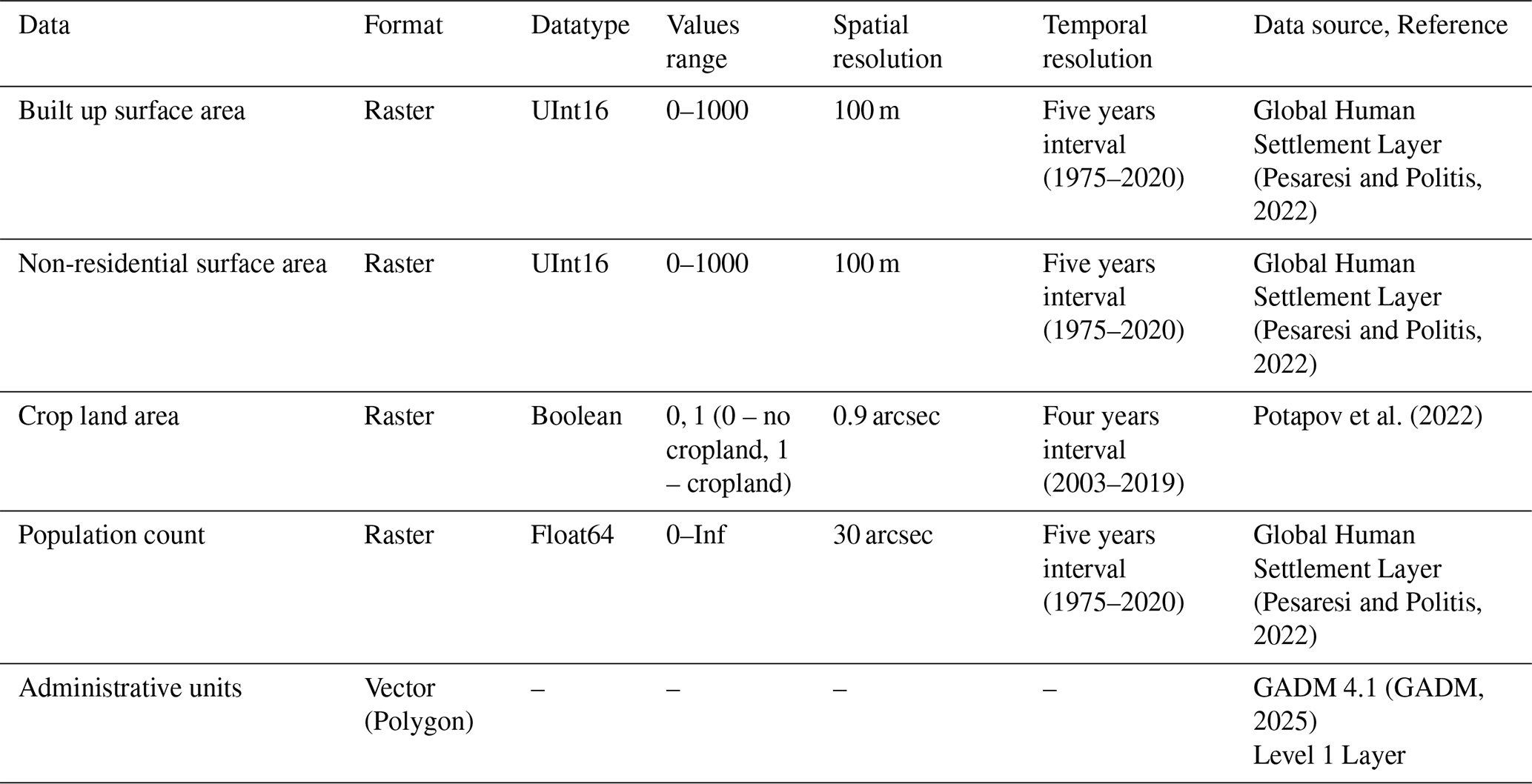
The spatially distributed sectoral GDP map was created in two steps (Fig. 1). First, we classified country level GDP data into three sectors: the agriculture, service, and industry sector, and they are downscaled to a spatial resolution of 30 arcsec based on population data, referred as population-based map (PB-method). Second, downscaled estimates are reallocated to the corresponding land use fraction maps derived from satellite products, referred to as land-use-based map (LUB-method). For both the agriculture and service sectors, we generated PB-method and subsequently reallocated them using land-use data. This two-step allocation is necessary because GDP is generally correlated with population distribution (Chen et al., 2022; Kummu et al., 2025), and service-sector GDP, in particular, is strongly influenced by urban agglomeration effects (Morikawa, 2011). However, previous studies have shown that at high spatial resolutions, population data alone may not adequately preserve these correlations (Murakami and Yamagata, 2019; Ru et al., 2023). Therefore, integrating land-use information is essential to ensure spatial consistency. Unlike the agriculture and service sectors, industry sector GDP doesn't necessarily follow population distribution. It often expands into suburban or rural areas with low population density (Zhuang and Ye, 2023). Accordingly, we bypass the PB-method step and directly allocate country-level industrial GDP to land use data. The List of the datasets used in this method is shown in Table 1.

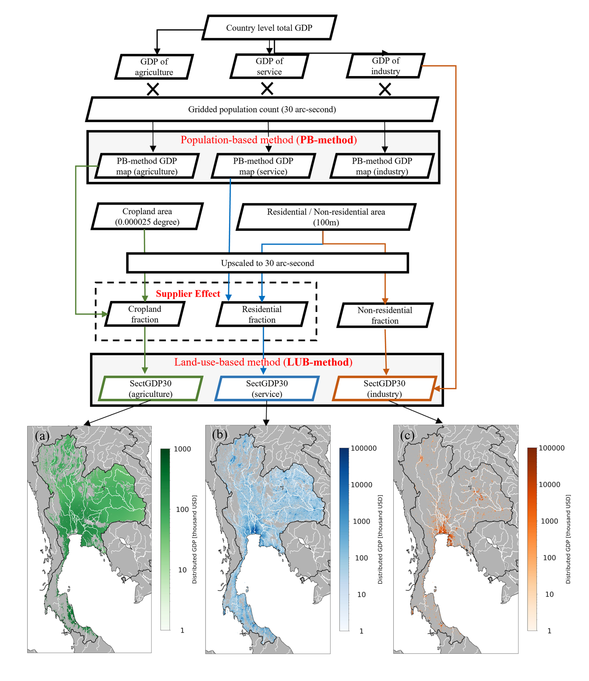
Figure 1 Flowchart of (top) data processing and (bottom) creation of spatial distributed gross domestic product (GDP) maps of Thailand for the (a) service, (b) industrial, and (c) agricultural sectors.

Table 1 List of the datasets used in this study.

2.1.1 Population-based sectoral GDP

In the first step, country-level GDP was partitioned into three sectors and then spatially distributed in proportion to population data at a spatial resolution of 30 arcsec. We used GDP data published by the World Bank (2023), which includes both annual GDP values and their sectoral ratios for the service, industrial, and agricultural sectors, and the Global Human Settlement Layer (GHSL) population grid (R2023; Pesaresi and Politis, 2022) as the source of the global gridded population map. The definition of each sector is shown in Table 2. This downscaling method has been widely employed in previous studies (Kummu et al., 2018; Murakami and Yamagata, 2019) and will be utilized in a later section for comparison with the new method proposed in this study.

2.1.2 Sectoral land use fraction map

In the second, step, we reallocated PB-method to global sectoral land use fraction map. We generated a sectoral land use fraction map classified into three sectors (service, industry, and agriculture) and three land use type maps with different spatial resolutions: residential (RES), non-residential (NRES), and cropland (CROP). To distinguish RES and NRES areas, we used Global Human Settlement Layer (GHSL) (Pesaresi and Politis, 2022) built-up surface (R2022) data. This layer has 100 × 100 m resolution; each pixel has a value of 0–10 000 m² and residential or non-residential areas may be present within one pixel. For the CROP area, we used the global map of cropland extent (Potapov et al., 2022), provided by Global Land Analysis & Discovery, which has a global spatial resolution of 0.9 arcsec. Maps with the three classes were resampled and combined into a single global sectoral land use (residential, non-residential, and cropland) fraction map at 30 arcsec resolution.

First, we upscaled the land use maps and simultaneously converted the value of each pixel in both maps into the sectoral fraction within one pixel. In each pixel, RES and NRES had values of 0–10 000 m² and CROP had a value of 0 or 1 (not cropland or cropland). We upscaled the land use maps to 30 arcsec resolution from RES and NRES at a resolution of 100 × 100 m and CROP at a resolution of 0.9 arcsec using the GDAL averaging method (GDAL/OGR contributors, 2024). Using the 30 arcsec maps, we calculated the area attributed to each land use type in one pixel with a size of 1 × 1 arcsec and obtained land use fractions for each pixel. Because RES/NRES and CROP had different data sources, the total of the three land use type fractions was greater than one in some pixels. Therefore, we assumed that the CROP fraction could fill only areas that were not designated as RES or NRES. Under this assumption, we modified the CROP fraction in each pixel as follows:

$$\begin{array}{}\text{(1)}& {\mathrm{MCROP}}_i=min\left({\mathrm{CROP}}_i,\left(\mathrm{1}-{\mathrm{RES}}_i-{\mathrm{NRES}}_i\right)\right)\end{array}$$

where MCROP_i is the modified CROP fraction in pixel i, CROP_i is the original CROP fraction, RES_i is the RES fraction, and NRES_i is the NRES fraction.

After this modification, RES, NRES, and MCROP were considered to represent the service, industrial, and agricultural land use sectors, respectively.

2.1.3 Land-use-based agriculture sector GDP

To better reflect the spatial structure of production activities, we introduce the supplier effect, which assumes a beneficiary-supplier relationship. Specifically, agricultural production occurring in peri-urban or rural areas surrounding major population centers is regarded as supplying food and resources to those urban beneficiaries. These agricultural zones, while themselves sparsely populated, are functionally integrated with the urban economy. Therefore, they are expected to exhibit higher GDP values than similarly sparse regions that are not spatially or economically connected to urban demand. To capture this spatial interdependence, the supplier effect applies a distance-decay reallocation from beneficiary pixels in PB-method to nearby supply-side pixels, namely those identified as MCROP. Technically, this is implemented as a linear decay function, in which full weight is given within an inner threshold of 150 km, and weight decreases linearly to zero at an outer threshold of 300 km.

$$\begin{array}{}\text{(2)}& \begin{array}{rl}{w}_{ij}=& \text{ if }{d}_{ij}\le d_{\mathrm{in}}:\mathrm{1};\\ & \text{ if }{d}_{\mathrm{in}}<d_{ij}\le d_{\mathrm{out}}:\mathrm{1}-(d_{ij}-d_{\mathrm{in}})/d_{\mathrm{in}};\\ & \text{ if }{d}_{ij}>d_{\mathrm{out}}:\mathrm{0}\end{array}\end{array}$$

Table 2 Definition of each sector, based on the International Standard Industrial Classification (ISIC) Rev 4, in the GDP data by the World Bank (2023).

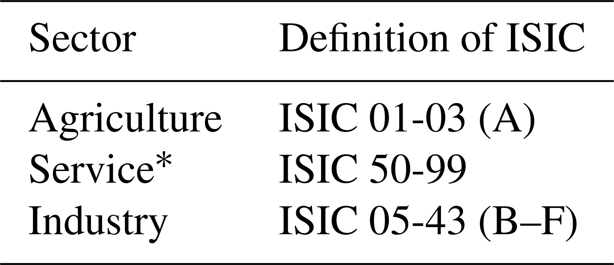
^* Note that only the Service sector is based on ISIC Rev. 3.

2.1.4 Land-use-based service sector GDP

Similarly, the PB-method of the service sector is reallocated to residential areas (RES) by applying the supplier effect. The rationale here differs slightly from that for agriculture. Grid-scale population data (e.g., at 30 arcsec resolution, or approximately 1 × 1 km per pixel) are too fine to represent realistic service usage, since people commonly travel more than 1 km by car or public transportation to access services (Ciccone and Hall, 1996). Therefore, this reallocation is designed to represent commuting patterns, where service activities in peri-urban zones support nearby urban demand centers. In this context, we use a supplier effect with an inner threshold of 25 km (representing high-intensity interaction) and an outer threshold of 50 km, beyond which service contributions are assumed negligible.

2.1.5 Land-use-based industry sector GDP

We distributed the industry sector GDP in each country by multiplying the distributed GDP per pixel by the NRES in each pixel. Thus, the distribution was performed for each country, as follows:

$$\begin{array}{}\text{(3)}& {\displaystyle }\begin{array}{rl}{\text{Industry GDP per pixel}}_{\mathrm{country}}& ={\text{Total Industry GDP}}_{\mathrm{country}}\\ & /{\sum }_{i=\mathrm{1}}^n{\mathrm{NRES}}_i\end{array}\text{(4)}& {\displaystyle }\begin{array}{rl}{\text{Industry GDP}}_{\mathrm{country},i}& ={\text{Industry GDP per pixel}}_{\mathrm{country}}\\ & \times {\mathrm{NRES}}_i\end{array}\end{array}$$

where is the Industry GDP per pixel of sector s in the country, is the total sectoral GDP of industry in the country, is the non-residential area in pixel i, n is the total number of pixels in the country, and is the distributed industry GDP in pixel i in the country.

2.2 Comparison of GDP distribution methods

We created two types of spatial distributed GDP map: population-based (PB-method), Land-use-based (LUB-method). The PB map was generated by downscaling the country GDP only in proportion to the gridded population count into a 30 arcsec map. The LUB-method was generated for each sectoral area and sectoral GDP per area. To assess the effectiveness of the proposed LUB mapping approach, we compared it against PB-method using the DOSE dataset (Wenz et al., 2023), which provides sectoral GDP estimates at the sub-national administrative unit level (GADM level 1). Both GDP maps (i.e., PB-method and LUB-method) were spatially aggregated from 30 arcsec resolution to the corresponding GADM Level 1 administrative boundaries to enable direct comparison with DOSE data. Comparison involved three steps: (1) Scatter plots were generated to evaluate the agreement between the aggregated values from each GDP map and corresponding sectoral GDP values from the DOSE dataset (agriculture, service, and industry) used as reference data. (2) For each method and sector, we computed the absolute value of the relative error between estimated and reference GDP values and derived the cumulative distribution functions to illustrate the distribution of errors across all administrative units. (3) We computed the difference in absolute relative errors between the LUB-method and PB-method to evaluate the improvement or deterioration in accuracy. For each administrative unit, this metric was calculated as:

$$\begin{array}{}\text{(5)}& \begin{array}{rl}\mathrm{\Delta }E& =E_{\mathrm{LUB}}-E_{\mathrm{PB}},\\ & \text{ where }E={\displaystyle \frac{\left|{\mathrm{GDP}}_{\mathrm{estimate}}-{\mathrm{GDP}}_{\mathrm{DOSE}}\right|}{{\mathrm{GDP}}_{\mathrm{DOSE}}}}\end{array}\end{array}$$

A negative value of (ΔE) indicates that LUB-method is closer to the reference than PB-method (i.e., an improvement), while a positive value indicates a deterioration in accuracy compared to PB-method. The comparison was conducted using only administrative units for which all three sectoral GDP values were available for the year 2010. In total, the comparison included 1165 administrative units across 57 countries.

3 Results

We developed three GDP maps for service, industry, and agriculture sectors in 2010, 2015, and 2020. We excluded other years because of the low coverage of national GDP statistics in the World Bank data. Hereafter, the map generated using the LUB method within the Methods will be referred to as “SectGDP30”, and the map generated using the PB method will be referred to as “PB-method”. The maps of SectGDP30 are shown in Fig. 2a, b, and c. Additionally, to clarify the difference of spatial distribution among sectors, we showed (Fig. 2d) the map of the largest GDP sector in each grid in the world. Globally, the distribution of economic sectors generally correlates with population distribution, with concentrations observed in urban centers. However, variations exist in the detailed distributions. The service sector's distribution predominantly concentrates in urban areas across countries, consistent with population distribution patterns and the use of residential data. In contrast, industrial GDP, proxied by non-residential areas, shows a tendency toward greater concentration in coastal regions. Conversely, agricultural GDP, while exhibiting some correlation with population distribution, is characterized by a more expansive distribution in inland areas compared to the service sector.

Examining individual countries allows for the identification of more specific differences in the distribution of each sector at a finer scale, shown in Fig. 3. In the figure of Japan, Japan's three major metropolitan areas – Tokyo, Osaka, and Aichi – show variations in sectoral distribution, despite their common characteristic of high population concentration. In the GDP map, the service sector predominates in the coastal areas of Tokyo and Osaka, which are marked by high population and service industry presence. In contrast, Aichi's coastal regions exhibit a widespread predominance of industrial GDP. Industrial GDP is not uniformly distributed across the entire Aichi area. Within Aichi, the more inland urban center, such as the Nagoya area, shows a prevalence of the service sector, with industrial GDP concentrated in coastal areas. These findings align with Aichi's higher proportion of industrial GDP compared to Tokyo and Osaka (Wenz et al., 2023, and the formation of an extensive industrial belt along its coastal regions. This dataset facilitates the depiction of detailed distributional differences within these areas.

When comparing central Bangkok with its southeastern region, a similar pattern emerges as a case in Japan. The southeastern area, specifically the Eastern Seaboard and Eastern Economic Corridor (EEC) centered around Laem Chabang Port, has developed as an industrial hub. In this region, industrial GDP predominates over service sector GDP. Regarding the distribution of agricultural GDP, Japan shows fewer pixels where agricultural GDP is dominant, largely because much of its agricultural land is located relatively close to urban areas. However, in Thailand and France, extensive areas with dominant agricultural GDP are observed around metropolitan centers like Bangkok and Paris. For instance, Fig. 4a, which shows only agricultural GDP for France, illustrates that agricultural GDP is minimally developed around densely populated Paris. Conversely, it depicts widespread agricultural activity in the less populated surrounding regions.

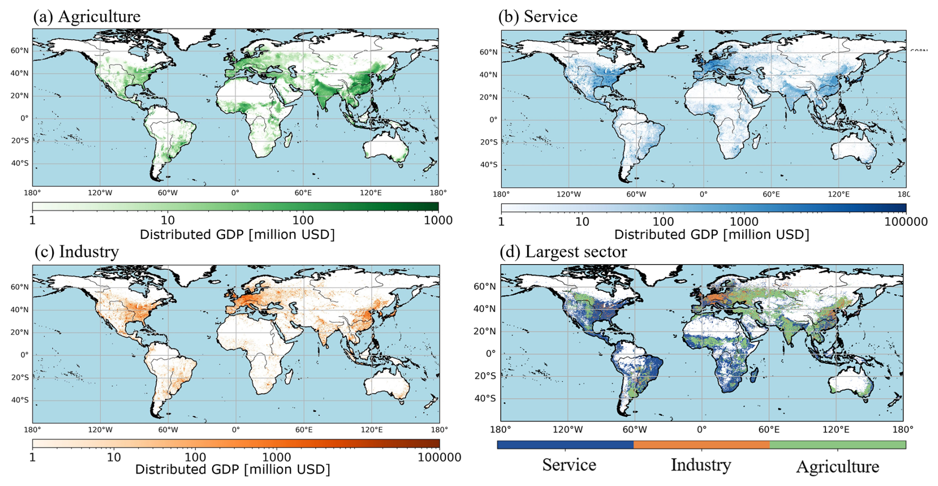
Figure 2 The sectoral GDP maps of (a) service sector, (b) industry sector, (c) agricultural sector, (d) the map of the largest GDP sector in each grid of 30 arcsec.

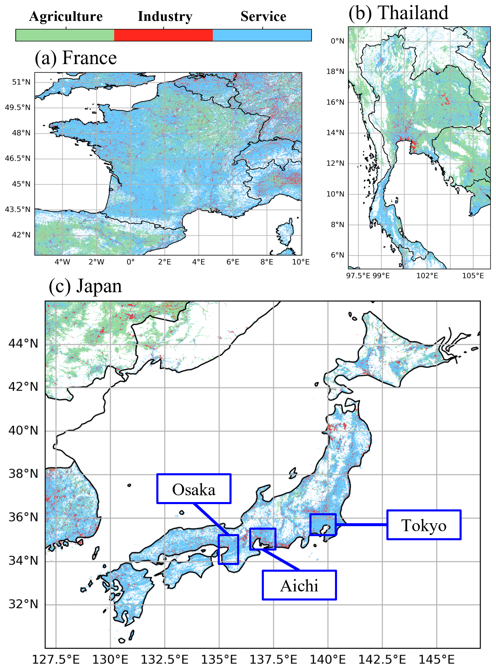
Figure 3 The map of the largest GDP sector in each grid of 30 arcsec in (a) France, (b) Thailand, and (c) Japan.

To validate the accuracy of this GDP map, we conducted a comparative analysis with DOSE, a dataset providing sectoral GDP figures at the sub-national administrative unit level. For this validation, the 30 arcsec resolution GDP map was spatially aggregated according to the GADM dataset's Level 1 administrative divisions, which are used by DOSE. The aggregated GDP values for each administrative unit were then calculated and compared with DOSE's figures.

The results are presented in Fig. 4a, b, and c. These three scatter plots indicate that SectGDP30 exhibits a similar distribution to actual sub-national scale sectoral GDP (R² > 0.9 in all the sectors). When examined by sector, many administrative units with discrepancies in service and industrial GDP show an underestimation compared to actual data. Given that the total GDP per sector at the national level aligns with real data in this study, this discrepancy likely results from over-distributing GDP in a few administrative units within certain countries, leading to an underestimation in many other smaller administrative units. While service and industrial GDP inherently concentrate in specific local areas, and this GDP map depicts that, some countries show an excessive concentration in particular regions. This trend is less apparent in agricultural GDP, which exhibits less localized distribution, and no strong pattern of overestimation or underestimation was observed.

Next, we compared the results from SectGDP30 with the PB-method. The comparison method involved using sectoral GDP figures for each administrative unit, as before, and calculating the cumulative distribution of the differences from DOSE's figures. This result is presented in Fig. 4d. Sectoral analysis reveals that the industrial sector shows the most significant improvement when compared to PB-method. As previously mentioned, industrial GDP distribution often exhibits localized concentrations even in sparsely populated areas. This suggests that a method using only non-residential land use information and concentrating distribution over relatively small areas is more appropriate than PB-method, which relies on population distribution data.

The service sector shows a slight decline in accuracy compared to PB-method. In the service sector, overall regional results showed a slight decrease in accuracy for SectGDP30 compared to PB-method. However, some regions exhibited improved accuracy with SectGDP30. Fundamentally, there is minimal difference between SectGDP30 and PB-method as the spatial distributions of residential areas (upon which SectGDP30 relies) and population (upon which PB-method relies) largely coincide.

Conversely, SectGDP30 incorporates Supplier effect, reallocating each grid's GDP to residential areas within a 50km radius. This results in a smoother connection of urban and rural area distribution differences compared to PB-method. This effect is evident in the Alpine regions of Switzerland (CHE), specifically in administrative level districts such as Uri, Wallis, Graubunden, and Glarus. While these Swiss Alpine areas have a significant population, residential areas are limited, and actual statistical service GDP is not high. Therefore, in Switzerland, service GDP should be distributed not based on simple population distribution but rather in the plains north of the Alps, where numerous residential areas exist. This case demonstrated an improvement in SectGDP30 accuracy. Agricultural GDP also shows an improvement compared to PB-method, with an increase in the number of administrative units exhibiting smaller errors.

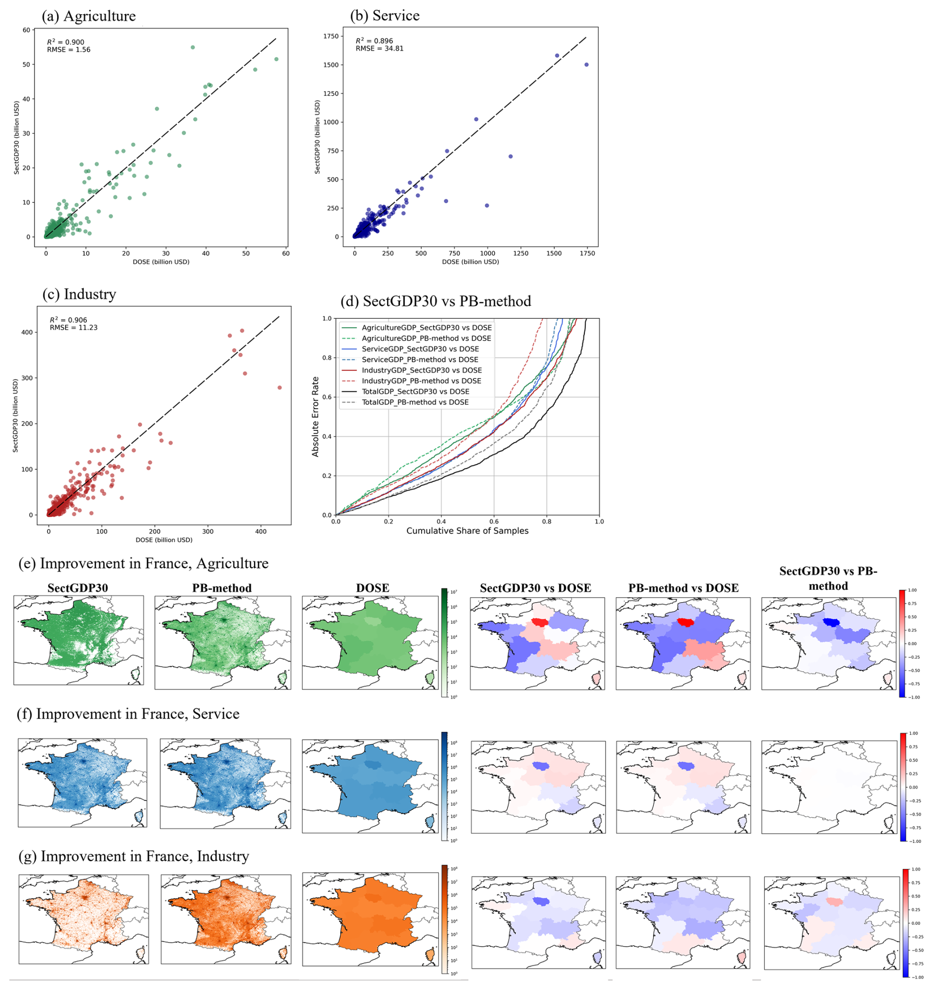
Figure 4 The scatter graphs of the municipality GDP for (a) service sector (b) industry sector (c) agriculture sector and (d) the cumulative distribution of the errors between DOSE and SectGDP30 and between DOSE and PB-methods for each sector.

4 Discussion – Business interruption loss estimation for the 2011 Thailand flood

To assess how the improvement of the GDP map affects the result of flood loss estimation, an additional analysis of estimating business interruption losses resulting from the actual flood event in Thailand in 2011 by the new sectoral GDP map was conducted. Following established definitions of economic losses from prior studies (Tanoue et al., 2020; Rose, 2004), economic impacts can be categorized into three main types: damage, direct economic loss, and indirect economic loss. This additional analysis focused exclusively on estimating Business Interruption loss (BI loss) among these three economic impacts due to the lack of information necessary for the estimation of the other components.

To calculate BI loss, we prepared hazard, exposure, and vulnerability data. As the hazard, we used two inundation period maps of the target event in Thailand, based on simulation and satellite observations. The simulation-based inundation period map was generated using the Catchment-based Macro-scale Floodplain (CaMa-Flood) global riverine inundation model (Yamazaki et al., 2011). To obtain an inundation map based on the simulation by CaMa-Flood, CaMa-Flood used daily runoff data generated by a reduced-bias meteorological forcing dataset at 15 arcmin resolution, and S14FD-Reanalysis data (Iizumi et al., 2017) to simulate the daily inundation depth at 15 min resolution. Because S14FD is a bias-corrected dataset, we used daily inundation depth values without bias correction, such that the inundation period may be calculated directly from the daily inundation depth (Taguchi et al., 2022). Then, we downscaled the 15-arcmin daily inundation depth to 30 arcsec resolution and calculated the inundation period as the number of days in which the inundation depth exceeded 0.5 m in each pixel. We also used an inundation period map based on Terra/Moderate Resolution Imaging Spectroradiometer (MODIS) images, which is publicly available on the Global Flood Database (Tellman et al., 2021). We referred to the former hazard map as “CaMa-Flood” and the latter map as “MODIS” in this study. The days between August and December in 2011 were only counted as inundation days for matching the inundation period by CaMa-Flood simulation and that by MODIS observation, which started from August and ended around the end of December.

As exposure, we used two spatial distributed GDP maps at 30 arcsec resolution for comparison, SectGDP30 and PB-method. As a vulnerability, we considered a recovery coefficient, which decided the ratio of the length of recovery period which is required until business restart to the inundation period. This value reflects the system vulnerability of the city. We used 2 as a recovery coefficient, which was used in previous study on a global scale (Taguchi et al., 2022). As for the recovery period as vulnerability, we used the method of Tanoue et al. (2020). The recovery period RP_i, when the production in a pixel is assumed to have recovered linearly from zero at the end of the flood period to the same level of production before the flood, was obtained by multiplying the inundation period by a coefficient (= 2 in this study). Thus, the recovery period was assumed to take twice as long as the inundation period. Finally, BI loss was estimated by the method described by Tanoue et al. (2020), as follows:

$$\begin{array}{}\text{(6)}& \text{BI loss}={\sum }_{i=\mathrm{1}}^N{\sum }_s^{\mathrm{3}}\left\{\left({\mathrm{IP}}_i+{\displaystyle \frac{{\mathrm{RP}}_i}{\mathrm{2}}}\right)\times {\displaystyle \frac{{\mathrm{AGDP}}_{i,s}}{Nd}}\right\}\end{array}$$

where i, N, and s are the pixel number, total number of pixels in the inundated area, and sector number (1 = service, 2 = industry, and 3 = agriculture), respectively; IP_i, RP_i, AGDP_i,s, and Nd are the inundation period, recovery period at pixel i, annual GDP of pixel i and sector s, and the number of days in a year.

And we obtained the total BI losses by summing BI losses of all the grids in the target area.

The results of the BI loss estimation were shown in Fig. 5. We compared the calculated BI losses with the actual economic loss reported in the PDNA (The World Bank, 2011). In this report, both damage and loss were estimated. Damage is due to the destruction of physical assets and loss is caused by foregone production and income and higher expenditures in the definition in the report. This means that the loss in the report included both business interruption loss and other additional expenditures and costs. Because there was not any other reported loss which only focused on BI loss, we compared with the loss, including other components, in this report.

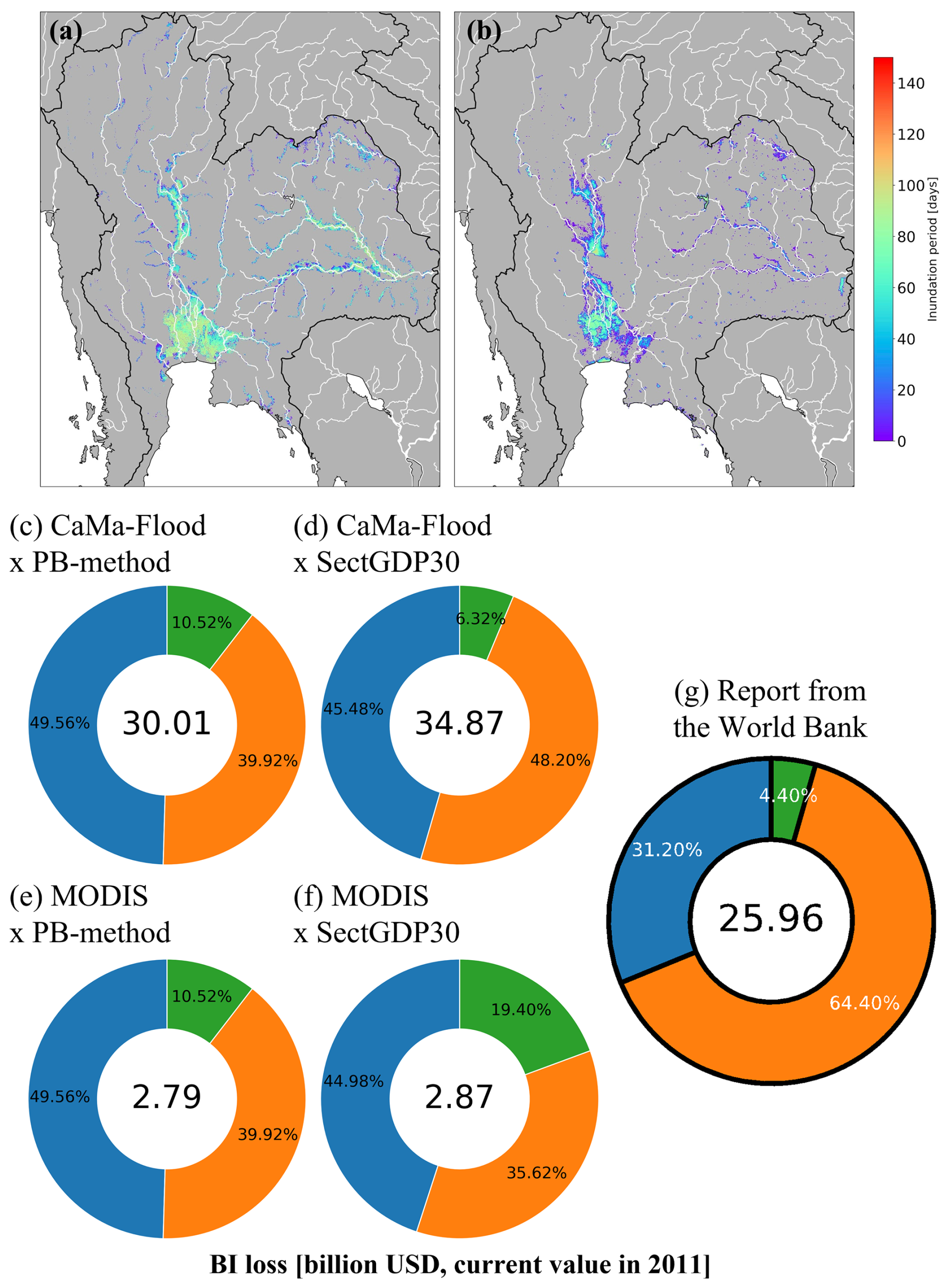
Figure 5 Spatial distribution of the inundation period of the 2011 Thailand flood, obtained from (a) Catchment-based Macro-scale Floodplain (CaMa-Flood) simulation and (b) Moderate Resolution Imaging Spectroradiometer (MODIS) observation data, and the simulation Business interruption losses (USD billion, current value in 2011) due to the 2011 Thailand flood, estimated by combining hazards and exposures; the total loss is written in the center of each circle. (c) CaMa-Flood and PB-method, (d) CaMa-Flood and SectGDP30, (e) MODIS and PB-method, (f) MODIS and SectGDP30, and (g) the World Bank report (2011).

Firstly, comparing the losses by the different hazard data with the same exposure, SectGDP30, the service sector loss according to CaMa-Flood (USD 15.86 billion) was over 12-fold larger than that according to MODIS (USD 1.29 billion). This large difference was caused by the shorter average inundation period and smaller flood area in MODIS than in CaMa-Flood. MODIS is known to tend to fail to capture the flood extent in urban areas with high densities of tall buildings and that leads to the underestimation in inundation. In addition to different total losses, ratios of industry sector loss to the total loss differed between two results: 48.20 % according to CaMa-Flood and 35.62 % according to MODIS. This result showed the sectoral ratio of the loss can be changed depending on spatially different hazards. It is caused by the fact that SecGDP30 can show the different spatial distribution of each sectoral GDP, while municipality-level statistics cannot show the spatial distribution in a fine resolution. This sectoral difference was newly found by this study since the traditional population-based GDP map also could not show this difference between sectors.

Comparing the results using CaMa-Flood and SectGDP30 with the World Bank Report figures (Fig. 5d and g), SectGDP30 more accurately represents the smaller proportions of agricultural damage compared to when PB-method is used (Fig. 5c). This indicates that SectGDP30 can effectively constrain the allocation of agricultural GDP in areas with high population but limited agricultural land. Conversely, while the Report figures show a significant proportion for the industry sector, SectGDP30 results estimate the industry sector to be almost on par with the service sector. It showed the industry loss was underestimated although the hazard in the numerical simulation, by CaMa-Flood, captured the flood extent over the industrial sector area and the long-lasting inundation period. The reported value excludes assets damage but includes economic losses other than production reduction by direct contact with the flood, such as production stoppage due to shortages of raw materials induced by blocked roads. Therefore, if we assume that the new sectoral GDP map captured the industrial locations and they were successfully considered to be flooded, this underestimation is presumed to be caused by a lack of data reflecting the indirect production stoppage.

Related to this limitation of the indirect production stoppage, it is important to recognize that the methodology, including that of this paper and previous studies, which determines the GDP produced in each pixel using indicators such as GDP per unit area, overlooks the fact that labor supplied from remote locations is necessary for GDP production. To rephrase this with the example of a factory affected by a disaster: while the GDP output itself occurs at the factory's location, the workers who carry out the production reside in surrounding or remote areas. Therefore, if a disaster occurs in these remote residential areas, the GDP output should cease. However, pixel-based calculation methods would fail to represent this cessation of GDP output as long as the factory's pixel is unaffected. This is considered a non-negligible impact in regions where economic activity and residential areas are clearly separated, but quantifying this impact on a global scale is currently challenging. Alongside future research on regional differences in GDP per unit area, this remains a limitation that we must consider moving forward.

5 Data availability

The global sectoral GDP maps are publicly available via Zenodo at https://doi.org/10.5281/zenodo.15774017 (Shoji et al., 2025). The maps on Zenodo correspond to the SBCE maps in this paper and are stored as geotiff files. In total, there are nine maps in the dataset, for each sector (service, industry, and agriculture) and year (2010, 2015, and 2020).

6 Summary

This study developed a spatially distributed sectoral GDP map (SectGDP30) by leveraging recently available global, high-resolution land use datasets. This map demonstrates strong consistency (R² > 0.9) with actual sub-national statistical data and exhibits greater alignment with sub-national GDP statistics compared to conventional GDP maps (PB-method) that rely solely on gridded population maps.

For the industry sector, the methodology successfully distributed industrial GDP with better accuracy than population distribution alone. This was achieved by adopting “Non-residential areas” as a proxy, which effectively captures the localized nature of industrial GDP distribution in specific regions within each country. For agriculture, accuracy was improved over PB-method by distributing GDP based on farmland maps and assuming GDP generation in areas approximately 150–300 km from wide-area population centers. Regarding the service sector, incorporating population distribution within specific ranges, even when using residential land use map information, resulted in GDP being distributed only to actual built-up and designated residential areas. This approach achieved an accuracy comparable to the PB-method.

As an application of this dataset, business interruption (BI) loss estimation due to floods was conducted using the sectoral GDP map. This confirmed that the new sectoral GDP map can represent inter-sectoral differences in estimated BI losses, corresponding to varying spatial distributions of hazards. This validation underscores the importance of considering the spatially distinct distributions of sectors when estimating actual disaster damage. It also highlights the need for developing new estimation methods that account for the processes of GDP generation.

This new global sectoral GDP map serves as a foundational tool for estimating sector-classified economic losses. It meticulously considers the complexity of global land use patterns at a detailed level, enabling accurate calculation of sector-specific losses from various natural disasters on a global scale.