A surface ocean pCO₂ product with improved representation of interannual variability using a vision transformer-based model

The ocean plays a crucial role in regulating the global carbon cycle and mitigating climate change. Spatial and temporal variations of ocean surface partial pressure of CO₂ (spCO₂) influence the air–sea CO₂ flux through the difference between surface ocean and atmospheric pCO₂ (ΔpCO₂), which is further modulated by surface wind speed and gas exchange velocity. However, constructing a global spCO₂ data product that is able to resolve interannual and decadal variability remains a challenge due to the spatial sparsity and temporal discontinuity of observational data. This study presents an approach based on the Vision Transformer (ViT) model, combining high-quality observational data from the CO₂ Atlas (SOCAT) with multiple advanced global ocean biogeochemical models results to reconstruct a global monthly spCO₂ dataset (SJTU-AViT) at 1° resolution from 1982 to 2023. The approach employs the self-attention mechanism of the ViT model to enhance the modeling of the spatial and temporal variations of spCO₂, as well as incorporates physical-biogeochemical constraints from the derivative of spCO₂ with respect to key controlling factors as additional features. The incorporation of advanced ocean biogeochemical models during the training process allows the ViT-based model to capture more accurate spCO₂ variability in these data-sparse regions. Evaluations demonstrate that the new data product effectively captures spCO₂ variability at both global and regional scales, showing good consistency with SOCAT observations, long-term ocean station data, and global atmospheric CO₂ trends. The reconstructed spCO₂ demonstrates strong capability in reproducing spCO₂ anomalies during El Niño–Southern Oscillation (ENSO) events, particularly in the eastern Pacific Ocean, where it shows a correlation of −0.81 with the Niño 3.4 index and demonstrates high consistency with cruise data. Based on the SJTU-AViT dataset, the estimated global air–sea CO₂ flux patterns are consistent with known regional features such as strong uptake in the Southern Ocean and outgassing in the tropical Pacific. This study not only provides a new 42-year data product for advancing understanding of the ocean carbon cycle and global carbon budget assessments, but also introduces a new Transformer-based deep learning framework for Earth-system data reconstruction. The data product is publicly accessible at https://doi.org/10.5281/zenodo.15331978 (Zhang et al., 2025) and will be updated regularly.

1 Introduction

Global warming is primarily driven by the continuous increase in atmospheric greenhouse gas concentrations, with carbon dioxide (CO₂) being the dominant contributor (Friedlingstein et al., 2023). The ocean, as one of the largest carbon sinks in the Earth system, absorbs approximately 25 % of anthropogenic CO₂ emissions (∼2.80 Pg C yr⁻¹), playing a crucial role in regulating the global carbon cycle and climate change (Friedlingstein et al., 2023). However, the ocean's capacity to absorb CO₂ is not constant; rather, it is influenced by a complex interplay of atmospheric CO₂ concentration, ocean physical and biogeochemical processes, exhibiting significant spatiotemporal variability (Landschützer et al., 2016; Takahashi et al., 2002). Accurate estimation of oceanic CO₂ fluxes is therefore essential for understanding carbon cycle mechanisms and assessing the effectiveness of the ocean as a carbon sink.

Accurately quantifying air–sea CO₂ flux relies on precise estimates of sea surface CO₂ partial pressure (spCO₂). While the surface ocean CO₂ atlas (SOCAT) database (Bakker et al., 2016) provides a valuable foundation, observational coverage remains sparse and uneven, particularly in high-latitude regions and during winter months when harsh sea conditions limit measurements (Mackay and Watson, 2021). Existing approaches for estimating spCO₂ primarily fall into two categories: numerical biogeochemical modeling and data-driven methods. Traditional numerical biogeochemical models simulate spCO₂ by parameterizing physical and biogeochemical processes (Kern et al., 2024; Roobaert et al., 2022). However, due to the highly nonlinear dynamics of the oceanic carbon cycle and regional heterogeneity, numerical biogeochemical models still exhibit considerable uncertainties in reconstructing the spatiotemporal distribution of spCO₂ (Rödenbeck et al., 2015; Roobaert et al., 2022). Moreover, simplified parameterization of biogeochemical processes may lead to underestimation or overestimation of oceanic carbon uptake, ultimately affecting the accuracy of global carbon budget assessments (Resplandy et al., 2024).

To address these limitations, statistical interpolation and machine learning techniques have been increasingly employed to reconstruct spCO₂ distributions based on available observations (Rödenbeck et al., 2015). Statistical interpolation methods, such as regression-based approaches (Rödenbeck et al., 2015), Bayesian techniques (Valsala et al., 2021), and tree-based algorithms (Geurts et al., 2006), leverage the spatiotemporal correlation of spCO₂ observations and have achieved moderate success in some regions (Gregor et al., 2019). However, these methods struggle with poor reconstruction accuracy in data-sparse regions and do not fully capture the complex ocean carbon biogeochemical processes effectively (Hauck et al., 2023). Consequently, machine learning approaches have gained prominence in recent years. In particular, feedforward neural networks (FFNNs) have demonstrated superior reconstruction accuracy and have become one of the most widely used tools for spCO₂ and other ocean data estimation (Denvil-Sommer et al., 2019; Landschützer et al., 2013; Zeng et al., 2014). These methods yield root mean square errors (RMSE) of approximately 18 µatm in open ocean regions, aligning well with SOCAT observations (Gregor et al., 2019).

Despite recent advances, significant challenges remain in reconstructing spCO₂, particularly in capturing its interannual and decadal variability, which plays a pivotal role in modulating oceanic carbon uptake. Previous machine learning (ML)-based interpolations of pCO₂ may overly smooths the spatial patterns and interannual variability, which represents a potential limitation in capturing these features fully. Accurate characterization of this variability remains a central issue in the ocean carbon field. Furthermore, the widely used FFNNs method may introduce discontinuities at cluster boundaries due to the discrete nature of data grouping, impacting the representation of spCO₂ variability (Gregor et al., 2019). These discontinuities often require additional post-smoothing procedures, which may introduce artificial bias, thereby increasing reconstructed data uncertainty or suppressing real spatiotemporal variability (Gregor et al., 2019). More broadly, a persistent imbalance of approximately 1 Pg C yr⁻¹ remains in the global carbon budget, reflecting unresolved discrepancies between estimated sources and sinks on the global scale. One plausible contributor to this imbalance is the inadequate characterization of the interannual variability in oceanic carbon uptake (Friedlingstein et al., 2023). Therefore, this study develops a novel reconstruction method to more accurately capture interannual dynamics, alleviate artificial spatial discontinuities, particularly across cluster boundaries, and ultimately contribute to close the global carbon budget (Rödenbeck et al., 2015).

Transformer architectures, originally developed for sequence modeling in natural language processing, have demonstrated exceptional capabilities in capturing long-range dependencies and learning complex, nonlinear relationships across high-dimensional datasets. Their scalability and effectiveness in tasks such as machine translation, language understanding, and large language models (e.g., Chat-GPT) have established them as a cornerstone of modern artificial intelligence. Recently, these models have been extended to atmospheric science and oceanography, where they have shown promising performance in forecasting ocean states and extracting spatiotemporal patterns from large-scale environmental data. Given these advantages, Transformer-based frameworks offer considerable potential for data reconstruction in oceanography, where challenges such as sparse observations, multiscale variability, and strong spatiotemporal coupling demand flexible and powerful modeling approaches (Ji et al., 2025; Liu et al., 2024).

Against this backdrop, the image-based Vision Transformer (ViT) architecture, with its multi-head self-attention mechanism and high representational capacity, has emerged as a powerful tool for capturing the complex spatiotemporal features of oceanic environmental variables. This model is well-suited for reconstructing spCO₂, as it can integrate diverse environmental drivers such as sea surface temperature (SST), salinity (SSS), chlorophyll concentration (Chl a), mixed layer depth (MLD), and atmospheric CO₂ concentration. To enhance the physical constraints of spCO₂ reconstruction, this study incorporates ocean carbonate system sensitivities to key variables like SST, SSS, dissolved inorganic carbon (DIC), and total alkalinity (ALK) (Takahashi et al., 1993). In this context, multi-stage training strategies that combine simulated data from Earth system models and observational constraints have also proven effective in improving model robustness and accuracy. The spCO₂-based Shanghai Jiao Tong University aggregation Vision Transformer (SJTU-AViT) developed in this study effectively captures both spatial variations and interannual to decadal variability of ocean carbon dynamics at global scales. This contributes to enhancing our understanding of the temporal dynamics of oceanic carbon uptake and addressing imbalances in the global carbon budget.

2 Data and methods

2.1 Training data description

This study selects a range of input features for model training to comprehensively capture the dynamics of surface ocean spCO₂ variability through sensitivity tests and other spCO₂ data reconstruction studies (Denvil-Sommer et al., 2019; Landschützer et al., 2013; Zeng et al., 2014). The selected input features include SST, SSS, Chl a, MLD, and air CO₂. Additionally, we introduce physical constraints based on the relationship

$$\begin{array}{}\text{(1)}& \begin{array}{rl}\mathrm{\Delta }sp{\mathrm{CO}}_{\mathrm{2}}& \approx {\displaystyle \frac{\partial sp{\mathrm{CO}}_{\mathrm{2}}}{\partial \mathrm{DIC}}}\mathrm{\Delta }\mathrm{DIC}+{\displaystyle \frac{\partial sp{\mathrm{CO}}_{\mathrm{2}}}{\partial \mathrm{ALK}}}\mathrm{\Delta }\mathrm{ALK}\\ & +{\displaystyle \frac{\partial sp{\mathrm{CO}}_{\mathrm{2}}}{\partial \mathrm{SST}}}\mathrm{\Delta }\mathrm{SST}+{\displaystyle \frac{\partial sp{\mathrm{CO}}_{\mathrm{2}}}{\partial \mathrm{SSS}}}\mathrm{\Delta }\mathrm{SSS}\end{array}\end{array}$$

that the sensitivities of CO₂ partial pressure to SSS, SST, DIC, and ALK $(\frac{\partial sp{\mathrm{CO}}_{\mathrm{2}}}{\partial \mathrm{SSS}}$, $\frac{\partial sp{\mathrm{CO}}_{\mathrm{2}}}{\partial \mathrm{SST}}$, $\frac{\partial sp{\mathrm{CO}}_{\mathrm{2}}}{\partial \mathrm{DIC}}$, $\frac{\partial sp{\mathrm{CO}}_{\mathrm{2}}}{\partial \mathrm{ALK}})$ are included as input features in the deep learning model to reinforce spCO₂ physical-biogeochemical consistency (Takahashi et al., 1993). These parameters represent key physical, chemical, and biological factors influencing the distribution of spCO₂ in the ocean. All the input features are interpolated into a uniform 1°×1° spatial resolution and monthly temporal resolution.

The input datasets consist of long-term time series and high-resolution spatial data, ensuring both temporal and spatial consistency across variables (Table 1). SST data were obtained from the NOAA Optimum Interpolation SST (OISST) (version v02r01) dataset, spanning from 1982 to 2023 with daily resolution and a spatial resolution of 0.25° (Reynolds et al., 2007; Huang et al., 2021). SSS data were sourced from the Hadley Centre EN.4.2.2 (c14) dataset, covering the period from 1982 to 2023 with daily resolution and a spatial resolution of 0.25° (Good et al., 2013). Chl a data were derived from the European Space Agency Climate Change Initiative (ESA CCI) Ocean Colour (version 5.0) dataset, spanning 1997 to 2022 with daily resolution and a spatial resolution of 4 km (Jackson et al., 2017). For periods prior to 1997 and for 2023, we employed a climatology computed from the 1997–2022 Chl a record to ensure full temporal coverage. Ocean MLD data were obtained from the World Ocean Circulation Experiment (WOCE) Global Data Version 3.0, providing monthly climatology with a spatial resolution of 2° (de Boyer Montégut et al., 2004). Atmospheric CO₂ mole fraction (xCO₂) data were sourced from the NOAA Earth System Research Laboratories (ESRL) marine boundary layer (MBL) CO₂ product, covering the period from 1982 to 2023 with about 8 d resolution and meridional spacing (Dlugokencky et al., 2019). In this study, the meridional band product was mapped onto the model's 1°×1° global grid using latitudinal interpolation and longitudinal replication, generating continuous 2D fields suitable for model simulations.

Table 1 Summary of data sources and variable characteristics used in this study.

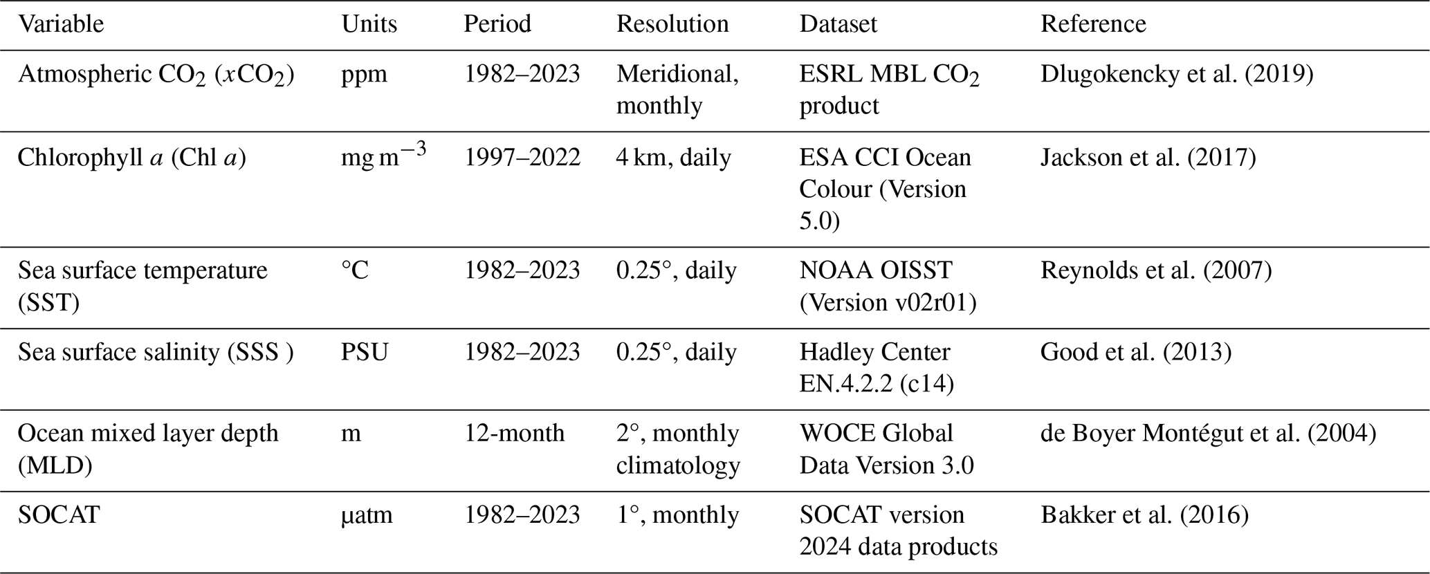
The monthly climatologies of $\frac{\partial sp{\mathrm{CO}}_{\mathrm{2}}}{\partial \mathrm{SSS}}$, $\frac{\partial sp{\mathrm{CO}}_{\mathrm{2}}}{\partial \mathrm{SST}}$, $\frac{\partial sp{\mathrm{CO}}_{\mathrm{2}}}{\partial \mathrm{DIC}}$, $\frac{\partial sp{\mathrm{CO}}_{\mathrm{2}}}{\partial \mathrm{ALK}}$ at a spatial resolution of 1° are included as additional input features, sourced from the ocean-driven global biogeochemical model simulations (Liao et al., 2020). These rate-of-change variables help to reflect the influences of temperature, salinity, alkalinity, and DIC on spCO₂, thereby enriching the deep learning model's representation of the underlying biogeochemical processes. Additionally, spCO₂ from the SOCAT database was used as the target variable for the model training and validation. The SOCAT dataset used in this study is version 2024 (Fig. S1 in the Supplement) which is interpolated into the uniform 1°×1° spatial resolution and monthly temporal resolution (Bakker et al., 2016).

The Coupled Model Intercomparison Project Phase 6 (CMIP6) model results are downloaded from the Lawrence Livermore National Laboratory node database (https://esgf31node.llnl.gov/projects/cmip6/, last access: 27 February 2025, at the time of this study). We selected a subset of 7 ESMs based on the availability of download access through our cluster and the availability of environmental variables (see Sect. S2 for details). The biogeochemical model adopted in this study is from the Geophysical Fluid Dynamics Laboratory (GFDL). The model includes Modular Ocean Model version 6 (MOM6), sea ice simulator version 2, carbon ocean biogeochemistry, and lower trophics version 2 (COBALT v2), which is collectively referred to as MOM6-COBALT2 (Adcroft et al., 2019; Stock et al., 2020). The model performance is thoroughly assessed, and it reproduces well-observed physical and biogeochemical features in the global ocean (Stock et al., 2020). More detailed model evaluations and configurations, including spin-up, atmospheric forcing, and initial conditions, can be found in Liao et al. (2020, 2024).

2.2 Model architecture

The deep learning model employed in this study is a Vision Transformer (ViT, Fig. 1), originally proposed by Dosovitskiy et al. (2020) for capturing spatial dependencies in large-scale image-like datasets. The design of ViT tackled the key limitation of the CNN-like methods, which implies the translation-invariant property of learned kernels. This property failed to learn the remote connections across regions among multiple variables (Liu et al., 2024). The ViT model employs a self-attention mechanism to capture long-term connections and complex spatial and temporal patterns (Nguyen et al., 2023), allowing it to dynamically adjust its receptive field and capture both localized details and large-scale variations. As a result, the model is able to provide a more comprehensive characterization of the relationships between spCO₂ and oceanic variables across spatial scales.

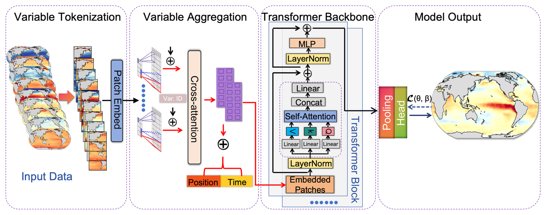
Figure 1 Schematic of the Vision Transformer (ViT)-based framework for spCO₂ reconstruction. The framework includes four main steps. The first is variable tokenization, where the input oceanographic variables (e.g., SST, SSS, Chl a, MLD, and atmospheric CO₂) are divided into spatial patches and passed through a convolutional embedding layer. The second step is variable aggregation, where multiple variables are aggregated into one vector through the cross-attention mechanism. The third step is Transformer backbone, where the data are passed through stacked Transformer blocks that incorporate multi-head self-attention, layer normalization, and feedforward neural networks to capture complex spatiotemporal dependencies. The final step is model output, where a pooling head aggregates the learned representations and generates the spCO₂ fields.

The ViT-based framework for spCO₂ reconstruction includes four main steps. The first is variable tokenization, a process that involves partitioning the input data into local regions. Each region is treated as an image patch for subsequent processing and feature extraction (Dosovitskiy et al., 2020). These input variables are standardized using variable-wise mean-variance normalization and formatted into a multi-channel input to ensure feature extraction occurs on a unified scale. Then, the ocean fields are segmented into fixed-size image patches. For example, the SST field (180×360) is divided into non-overlapping 6×6 grids on every patch, resulting in 30×60 patches. The data in each patch is then projected into a high-dimensional vector through a patch embedding layer, preserving critical spatial structures and providing a suitable input representation for the Transformer framework.

The second step is variable aggregation, where a cross-attention mechanism is employed to integrate information across multiple environmental input variables (Vaswani et al., 2017). Given that different variables influence spCO₂ through distinct mechanisms, other methods like simple concatenation may obscure crucial dynamic relationships. The cross-attention mechanism enables the model to adaptively assign appropriate weights to different variables, emphasizing those that contribute most significantly to spCO₂ variations (Jaegle et al., 2021). To further enhance its ability to capture spatiotemporal dynamics, the model incorporates position encoding and time encoding at this stage, ensuring temporal consistency in the input data and improving the interpretability of ocean carbon cycle processes (Wu et al., 2021).

The third step is Transformer backbone, where the data are fed into a Transformer backbone composed of 10 stacked Transformer blocks. Each block integrates multi-head self-attention (16 heads), layer normalization (LayerNorm), and a feedforward neural network (MLP) (Dosovitskiy et al., 2020; Vaswani et al., 2017). The multi-head self-attention mechanism enables the model to learn long-range dependencies and capture complex spatial interactions by attending to multiple representation subspaces simultaneously – an essential feature for modeling the inherently spatiotemporal dynamics of oceanographic variables. To further enhance representation learning, linear transformation and concatenation operations (Linear & Concat) are employed across layers. These operations support deep feature fusion, enabling the network to integrate both fine-scale local variations and broader climate-driven signals.

The final step is the model output. This step incorporates a pooling head for dimensionality reduction, producing the global oceanic spCO₂ fields as the output. The loss function is minimized by comparing the reconstructed values against observational datasets, ensuring both physical consistency and numerical accuracy. The ViT-based model contains approximately 115 million parameters and was trained in parallel on eight NVIDIA RTX 4090 GPUs for up to 200 epochs with early stopping (patience = 10); each training epoch required roughly 10 min.

To enhance model performance, we employ a multi-stage training strategy. First, we pre-train the ViT-based model using the 7 CMIP6 model results to learn a general relationship between spCO₂ and the environmental variables (SST, SSS, Chl a, MLD, and air CO₂). We then fine-tune the ViT-based model using data from the ocean-driven global ocean biogeochemical models (e.g., MOM6-COBALT) and further refine it with SOCAT observations to improve accuracy and applicability. The incorporation of the CMIP6 model and advanced ocean biogeochemical models enhances the spCO₂ reconstruction by mitigating the data sparsity issue, particularly in regions with limited observations, such as the Indian Ocean and high-latitude areas. Through the use of transfer learning, the model can better leverage global climate data to fill gaps in observational coverage. The overall workflow of this multi-stage training strategy is summarized in Fig. 2, which also provides a schematic overview of the spCO₂ reconstruction workflow based on the ViT framework. The figure clearly visualizes the main steps, from data preprocessing through model training to evaluation (see detailed description in Sect. S5.1).

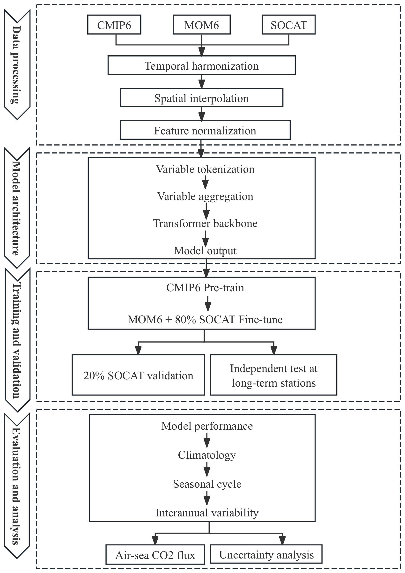
Figure 2 Workflow of the spCO₂ reconstruction using the ViT-based framework. The workflow consists of four major stages: (a) data processing, where CMIP6, MOM6, and SOCAT inputs are temporally harmonized, spatially interpolated, and normalized; (b) model architecture, where variables are tokenized, aggregated into spatio-temporal embeddings, and processed by a Transformer backbone to predict monthly spCO₂; (c) training and validation, involving CMIP6 pretraining, MOM6 and SOCAT fine-tuning, and evaluation against withheld SOCAT data and long-term stations; and (d) evaluation and analysis, where model performance metrics, climatology, seasonal cycles, and interannual variability are assessed, leading to downstream analyses such as air–sea CO₂ flux estimation and uncertainty analysis (see detailed description in Sect. S5.1).

2.3 Validation procedure and data

The SOCAT dataset was randomly divided into 80 % (277 528 samples) for training and 20 % (69 142 samples) for validation, using a fixed random seed (seed = 42) to ensure reproducibility. For the independent test at long-term stations, data from these stations were excluded, and the model was trained using the remaining SOCAT data. In the final results generation phase, the full SOCAT dataset was utilized to produce the spCO₂ estimates. These estimates are subsequently used for analyses of climatological states, seasonal variations, and interannual changes in spCO₂. For comparison with SOCAT, we used the monthly 1° gridded SOCAT product and evaluated our SJTU-AViT reconstruction on the same grid, without applying any additional spatial interpolation. Reconstructed values were masked where SOCAT is missing, and all skill metrics were computed only at grid-time points with valid SOCAT data. For the independent test at long-term stations, reconstructed values were extracted at the corresponding station locations using bilinear spatial interpolation, which incorporates information from surrounding grid cells to provide smoother and more representative estimates, and skill metrics were subsequently computed to evaluate model performance. Detailed information for these stations, including their names, geographic locations, observation periods, number of samples, and data sources, is provided in Table S3, and their locations are shown in Fig. S2 to facilitate visual interpretation. Subsequently, the climatological mean, seasonal variations, and interannual changes are calculated at each grid point where data are available. The processed SJTU-AViT data are then compared with the corresponding SOCAT observations in the following sections.

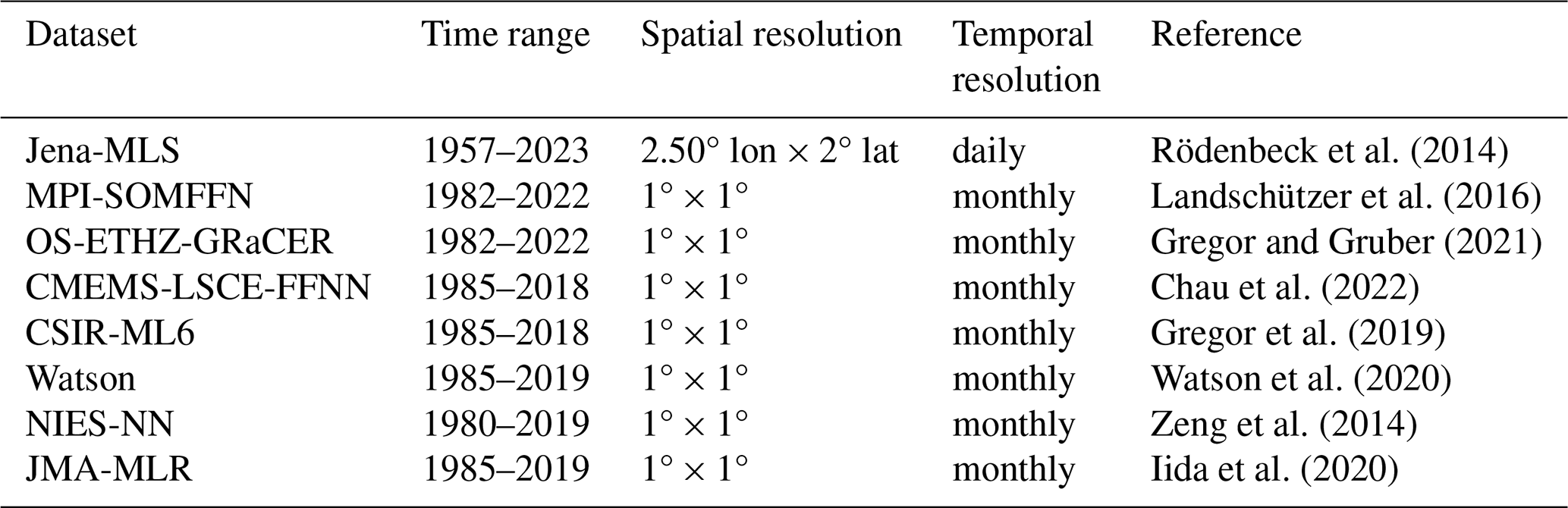
Table 2 References for global spCO₂ products used for comparison.

In the training process, we adopt the latitude-weighted mean squared error (MSE) as the loss function to ensure that the model accommodates the spatial variability caused by the Earth's curvature. The latitude-weighted MSE effectively emphasizes the prediction accuracy in low-latitude regions, which occupy a larger proportion of the Earth's surface (Nguyen et al., 2023; Willard et al., 2024). The loss function is computed as follows:

$$\begin{array}{}\text{(2)}& \mathrm{MSE}={\displaystyle \frac{\mathrm{1}}{N}}{\displaystyle \frac{\mathrm{1}}{H}}{\displaystyle \frac{\mathrm{1}}{W}}\sum _{t=\mathrm{1}}^N\sum _{h=\mathrm{1}}^H\sum _{w=\mathrm{1}}^W\mathit{\alpha }\left(h\right){\left(y_{t,h,w}-y_{\mathrm{obs},t,h,w}\right)}^{\mathrm{2}}\end{array}$$

where N is the total number of time points in the dataset, H and W are the numbers of latitudinal and longitudinal grid points, respectively, and t, h, and w represent the time, latitude, and longitude indices, respectively. $y_{\mathrm{obs},t,h,w}$ is the observed value, and $y_{t,h,w}$ is the predicted value. The term α(h) is the latitude weight.

In the validation process, we use multiple evaluation metrics, including mean bias error (MBE), mean absolute error (MAE), root mean square error (RMSE), and coefficient of determination (R²). These metrics have been extensively used in reconstructed data assessments and climate model evaluations. It is computed as follows:

$$\begin{array}{}\text{(3)}& {\displaystyle }& {\displaystyle }\mathrm{MBE}={\displaystyle \frac{\mathrm{1}}{n}}\sum _{i=\mathrm{1}}^n\left(y_{\mathrm{rec},i}-y_{\mathrm{obs},i}\right)\text{(4)}& {\displaystyle }& {\displaystyle }\mathrm{MAE}=\mathrm{1}/n\sum _{i=\mathrm{1}}^n\left|y_{\mathrm{rec},i}-y_{\mathrm{obs},i}\right|\text{(5)}& {\displaystyle }& {\displaystyle }\mathrm{RMSE}=\sqrt{\mathrm{1}/n\sum _{i=\mathrm{1}}^n{\left(y_{\mathrm{rec},i}-y_{\mathrm{obs},i}\right)}^{\mathrm{2}}}\text{(6)}& {\displaystyle }& {\displaystyle }{R}^{\mathrm{2}}=\mathrm{1}-\sum _{i=\mathrm{1}}^n{\left(y_{\mathrm{obs},i}-y_{\mathrm{rec},i}\right)}^{\mathrm{2}}/\sum _{i=\mathrm{1}}^n{\left(y_{\mathrm{obs},i}-\stackrel{\mathrm{‾}}{y_{obs}}\right)}^{\mathrm{2}}\end{array}$$

where n represents the number of data samples, y_rec,i denotes the reconstructed values, while y_obs,i and $\stackrel{\mathrm{‾}}{y_{\mathrm{obs}}}$ represent the observed values and their mean, respectively.

To evaluate the performance of the deep learning model (ViT-base Model) adopted in this study, we selected eight global ocean spCO₂ products (Table 2), nine independent observational stations (Fig. S2a), and SOCAT data. The chosen benchmark datasets include Jena-MLS, MPI-SOMFFN, OS-ETHZ-GRaCER, and five other data products (Table 2), which are widely used in the ocean carbon community. These data products cover periods from 1957 to 2023 at varying spatial resolutions from 1 to 2.50°, with temporal resolutions ranging from daily to monthly. The nine stations span various periods and effectively capture the spatial and temporal variability of ocean spCO₂. The diversity of the benchmark datasets provides a deeper understanding of the model's performance across different oceanic environments, thus further optimizing its predictive capabilities.

2.4 Air–sea CO₂ flux computation

We calculate the air–sea CO₂ flux (FCO₂, mol C m⁻² yr⁻¹) from the reconstructed spCO₂ using a standard bulk parameterization (Wanninkhof, 2014), given by the equation:

$$\begin{array}{}\text{(7)}& F{\mathrm{CO}}_{\mathrm{2}}=k_w\cdot K_{\mathrm{0}}\cdot \left(\mathrm{1}-f_{\mathrm{ice}}\right)\cdot \left(sp{\mathrm{CO}}_{\mathrm{2}}-ap{\mathrm{CO}}_{\mathrm{2}}\right)\end{array}$$

Here, the flux (FCO₂) is considered positive when CO₂ is outgassed from the ocean and negative when CO₂ is absorbed by the ocean. The fluxes are adjusted to account for the ice-free area of each pixel, with the sea ice cover data (f_ice) taken from Rayner et al. (2003). The gas transfer velocity of CO₂ (k_w) is computed using the parameterization of Wanninkhof (2014), which assumes a quadratic dependence on wind speed. The Schmidt number (Sc) required in this formulation is calculated following the temperature-dependent empirical formula provided by Wanninkhof (2014). The wind speed data is sourced from ERA5, with a 6-hourly temporal resolution spanning 1982–2023 and a 1° spatial resolution. To ensure consistency with global radiocarbon-based constraints (Graven et al., 2012; Müller et al., 2008; Sweeney et al., 2007; Wanninkhof, 2014), the scaling factor is set as 0.251 (Wanninkhof, 2014), which equals about a global mean transfer velocity of 16 cm h⁻¹. The solubility of CO₂ in seawater (K₀) is calculated as a function of SST and SSS (Weiss, 1974). The partial pressure of atmospheric CO₂ (apCO₂) is estimated using the mole fraction of CO₂ in dry air (xCO₂) from the ESRL MBL CO₂ product, with water vapor correction from Dickson et al. (2007).

2.5 ViT-based model uncertainty estimation

The uncertainty associated with our reconstructed spCO₂ product was estimated using the method proposed by Landschützer et al. (2014, 2018). The uncertainty of estimated spCO₂ for each grid cell was accumulated from the quadratic sum of four sources of uncertainties:

$$\begin{array}{}\text{(8)}& u_{sp{\mathrm{CO}}_{\mathrm{2}}}=\sqrt{u_{\mathrm{obs}}^{\mathrm{2}}+u_{\mathrm{grid}}^{\mathrm{2}}+u_{\mathrm{algorithm}}^{\mathrm{2}}+u_{\mathrm{inputs}}^{\mathrm{2}}}\end{array}$$

u_obs is the observational uncertainty inherited from observations. The SOCAT gridded product compiles the pCO₂ observations with WOCE flags A, B (uncertainty < 2 µatm), C, and D (uncertainty < 5 µatm). Adopting a conservative approach, we set the maximum value of u_obs to 5 µatm. u_grid is calculated as the standard deviation of the samples used for gridding spCO₂ in each grid cell (Roobaert et al., 2024a; Wu et al., 2025). u_algorithm is evaluated as the RMSE between the reconstructed and reference ocean model spCO₂ field.

In addition to the three uncertainty sources previously mentioned, this study also considers the cumulative uncertainty introduced by input variables (u_inputs). The uncertainties associated with these variables are calculated through Monte Carlo simulations (Wu et al., 2025). For each input variable, white noise following a normal distribution (N(0,u_xi)) is added, and spCO₂ is recalculated using the perturbed inputs. By repeating 100 times, the uncertainty for each input variable is then determined by calculating the standard deviation of the differences between the original spCO₂ and the spCO₂ values obtained after adding noise. Detailed procedures for determining these input uncertainties are described in Sect. S1 in the Supplement.

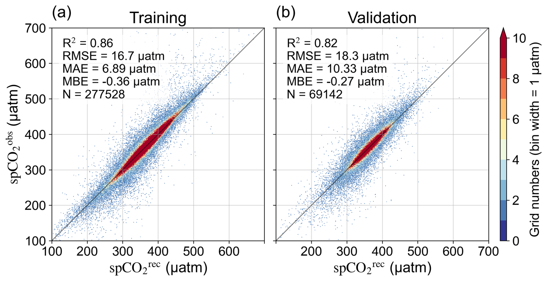
Figure 3 Performance evaluation of the ViT-based model for reconstructing the SJTU-AViT spCO₂ product. Density scatter plots illustrate the comparison between model-reconstructed sea surface partial pressure of CO₂ (spCO${}_{\mathrm{2}}^{\mathrm{rec}}$) and in situ SOCAT observations (spCO${}_{\mathrm{2}}^{\mathrm{obs}}$) during (a) the training phase (using 80 % of the samples) and (b) the validation phase (using 20 % of the samples). Statistical metrics, including the coefficient of determination (R²), root mean square error (RMSE), mean absolute error (MAE), mean bias error (MBE), and the number of samples (N), are provided to quantitatively assess model performance. The color bar indicates the number of data points within each bin, representing the density of observations. The spCO₂ in SJTU-AViT is interpolated to match the SOCAT observation locations and times in the comparison.

3 Results

3.1 Evaluation of ViT-based model performance

The SJTU-AViT product demonstrated robust performance and high accuracy in capturing spCO₂ variability (Fig. 3). In the training phase (Fig. 3a), the model achieved a high coefficient of determination (R²=0.86), with low root mean square error (RMSE = 16.70 µatm), an MAE of 6.89 µatm, and minimal mean bias error (MBE = −0.36 µatm), based on over 277 528 (80 %) samples. In the validation phase (Fig. 3b), the model maintained robust performance, with an R² of 0.82 and an RMSE of 18.30 µatm, indicating strong generalization ability and no sign of overfitting. Most predicted values lie close to the 1:1 line, particularly within the climatologically common spCO₂ range (300–420 µatm), as indicated by the high-density regions in Fig. 3. These results confirm the model's ability to accurately reconstruct large-scale spCO₂ patterns across diverse oceanic regimes. In addition, the sensitivity test indicates that the implementation of physical-biogeochemical constraints can significantly improve model performance, reducing the mean absolute error from 7.15 to 5.95 µatm.

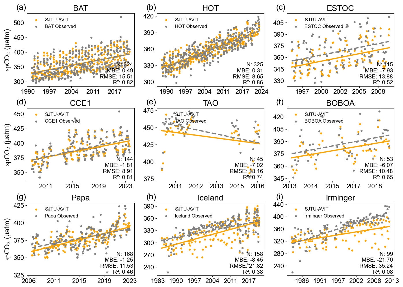
Figure 4 Independent test of spCO₂ variability between SJTU-AViT and in situ observations at different stations. These in situ data are independent data and are not used to train the model. The station description and location refer to Sect. S2 and Fig. S2. The spCO₂ in SJTU-AViT is interpolated to match the station locations and times in the comparison. For each panel, the number of samples (N), the mean bias error (MBE), root mean square error (RMSE), and correlation coefficient (R²) between the reconstructed and observed spCO₂ are displayed. The dashed and solid lines show the linear trend of SJTU-AViT and in situ data.

Independent test with in-situ buoy observations (which were not used to train the model) (Fig. 4) indicates that the model performs best in subtropical regions (e.g., HOT, BATS, CCE1, ESTOC, and Papa), accurately capturing both long-term trends (Fig. 4) and seasonal cycles (Fig. S3). At the HOT station, for instance, the model yields a minimal MBE of 0.31 µatm, a low RMSE of 8.65 µatm, and a high R²=0.86, and similar performance is observed at other subtropical stations, indicating the model's accuracy in data-rich, stable regions. In the equatorial Pacific Ocean, the model shows reasonable performance at the data-sparse TAO station in the Pacific Ocean, with a slight negative MBE (−7.02 µatm), an RMSE of 13.16 µatm, and an R² of 0.74, effectively capturing large-scale seasonal variability in equatorial upwelling-dominated environments (Fig. S3). Similarly, at the monsoon-influenced BOBOA station at the Bay of Bengal, where observations are also limited, the model captures overall variability with an MBE (−6.07 µatm), an RMSE of 10.48 µatm, and an R² of 0.65, indicating reasonable skill in capturing the overall variability driven by monsoonal forcing processes. In contrast, performance deteriorates at high-latitude stations and regions with strong dynamical variability. At the Irminger Sea and Iceland sites, the model exhibits large RMSE (35.24 and 21.82 µatm, respectively) and low correlations, with R² near zero. This suggests that the model has difficulty capturing rapid spCO₂ fluctuations or processes that are not well represented by the available input features. This discrepancy is likely due to high-latitude processes such as seasonal sea-ice variability and freshwater inputs, which are not fully represented in the current observational constraints.

In general, the evaluation confirms that the ViT-based method effectively generates essentially bias-free spCO₂ fields with no signs of overfitting, achieving high accuracy in low latitudes and open oceans, while performance declines at high latitudes.

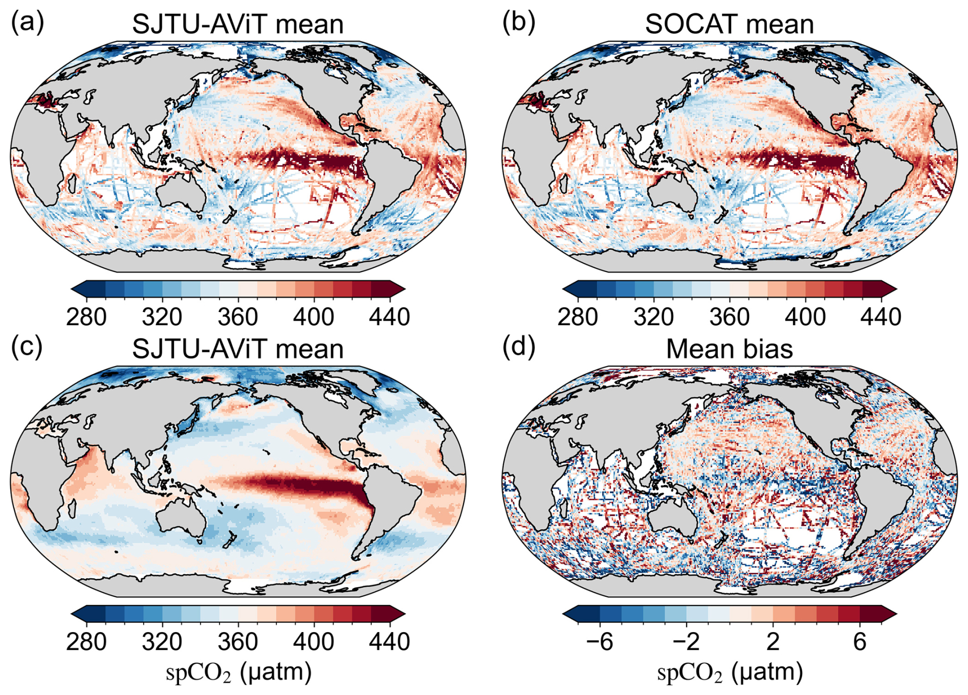
Figure 5 Comparison of long-term mean spCO₂ between SJTU-AViT and SOCAT over 1982–2023. (a) Long-term mean spCO₂ from SJTU-AViT on the SOCAT observation grid points. (b) Long-term mean spCO₂ from SOCAT. (c) Long-term mean spCO₂ from SJTU-AViT at all grid points. (d) Mean bias (SJTU-AViT minus SOCAT, panel a minus panel b) on SOCAT observation grid points. In panel a, SJTU-AViT values are first interpolated to match the spatial and temporal locations of SOCAT observations, after which the long-term mean is calculated at each grid point where data are available (see detailed computation in Sect. 2.3).

3.2 Evaluation of long-term climatology and annual means of spCO₂

The reconstructed spCO₂ product (SJTU-AViT) exhibits strong agreement with SOCAT observations in terms of long-term climatology, successfully capturing the large-scale spatial distribution of spCO₂ in the global ocean (Fig. 5a–c). This demonstrates strong consistency with previous climatology products (Landschützer et al., 2020; Takahashi et al., 2002). Elevated spCO₂ values are prominent in the tropical oceans (e.g., equatorial Pacific Ocean) and coastal upwelling regions, driven by the upwelling of CO₂-rich subsurface waters. In contrast, low spCO₂ levels are predominantly observed in mid-latitude gyre areas (e.g., the North Pacific Ocean) which is driven by subduction processes. The relatively low spCO₂ is present in the high-latitude regions, driven primarily by low temperature and a strong biological pump.

Compared with all SOCAT observation grid cells, the SJTU-AViT product exhibits good performance metrics in terms of long-term climatology, characterized by a low bias (MBE = −0.21 µatm, Fig. 5d), a low MAE of 5.95 µatm, a low RMSE of 7.44 µatm, and a notably high correlation coefficient (R=0.94). The small averaged bias suggests that the model does not exhibit systematic over- or under-estimation at the global scale, further validating its reliability in estimating the monthly and annual mean climatology of spCO₂. However, despite the small overall bias, the spatial distribution of bias shows significant regional variation (Fig. 5d). The larger biases (>4 µatm) are predominantly found in the coastal, tropical, and high-latitude oceans. The bias comparison between coastal and open oceans indicates the probability distribution function (pdf) for open ocean centers around 0.16 µatm, with 90 % of the biases falling between −12 to +10 µatm (Fig. 6b). Conversely, the pdf for coastal ocean (400 km distance from the coastline) bias centers around −1.44 µatm, with 90 % of the biases remain within the range of −18 to +14 µatm (Fig. 6c). The larger biases in the coastal ocean may stem from complex coastal physical-biogeochemical processes, such as terrestrial inputs, tidal mixing, and freshwater fluxes from rivers (Bauer et al., 2013; Cai et al., 2020; Roobaert et al., 2024b). These processes are often difficult to accurately capture in global-scale reconstruction models.

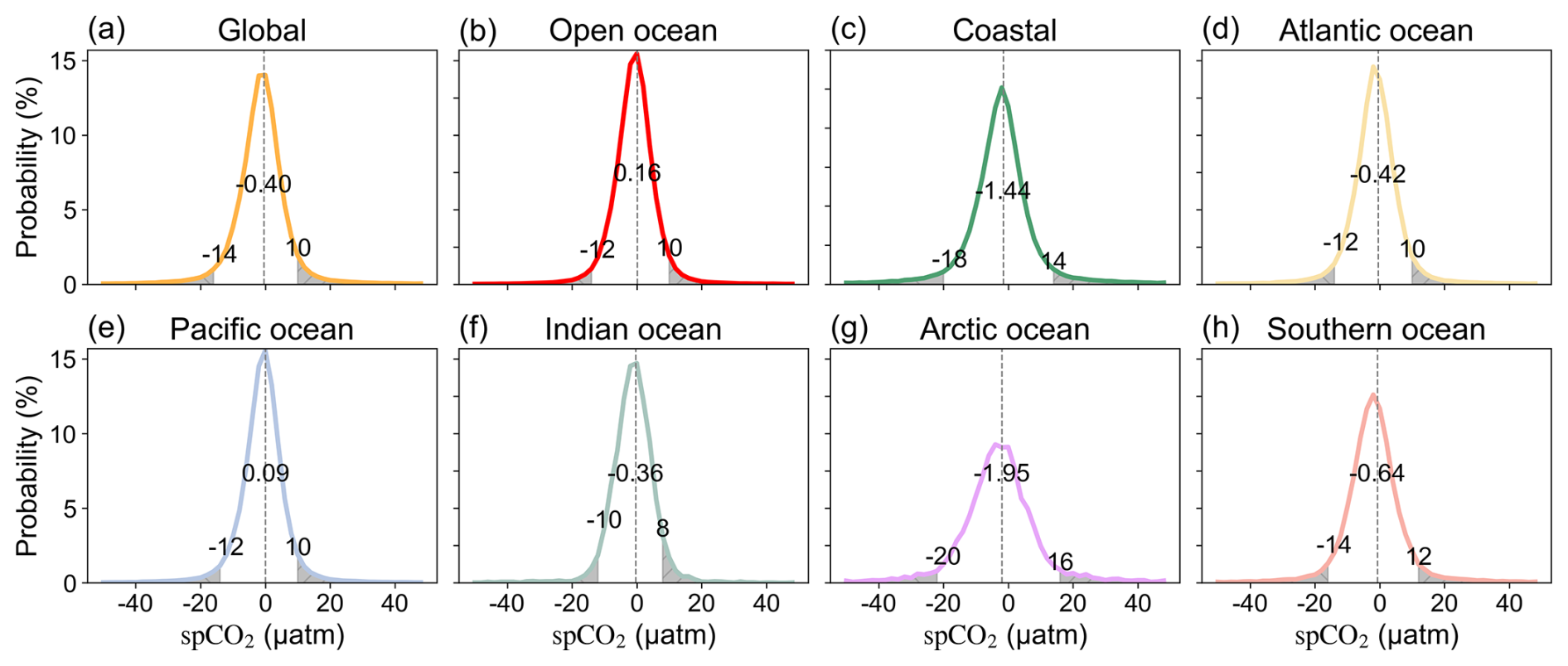
Figure 6 Bias probability density distributions of long-term mean spCO₂ for the SJTU-AViT product compared to SOCAT data across different ocean regions. (a) Global ocean, (b) Open ocean, (c) Coastal ocean, and (d–h) individual ocean basins. Coastal ocean is defined as the region within 400 km from coastline. The spatial extents of the ocean basins are shown in Fig. S2. The vertical dashed line represents the mean spCO₂ value for each region, with the 95 % and 5 % threshold points marked on either side of the mean. The values next to the dashed lines indicate the corresponding mean bias and the values at the two sides of dashed lines are 95 % and 5 % percentiles for each region. The spCO₂ in SJTU-AViT is interpolated to match the SOCAT observation locations and times in the bias computation (see detailed computation in Sect. 2.3). The asymmetry in the percentiles is due to the asymmetric shape of the probability density function.

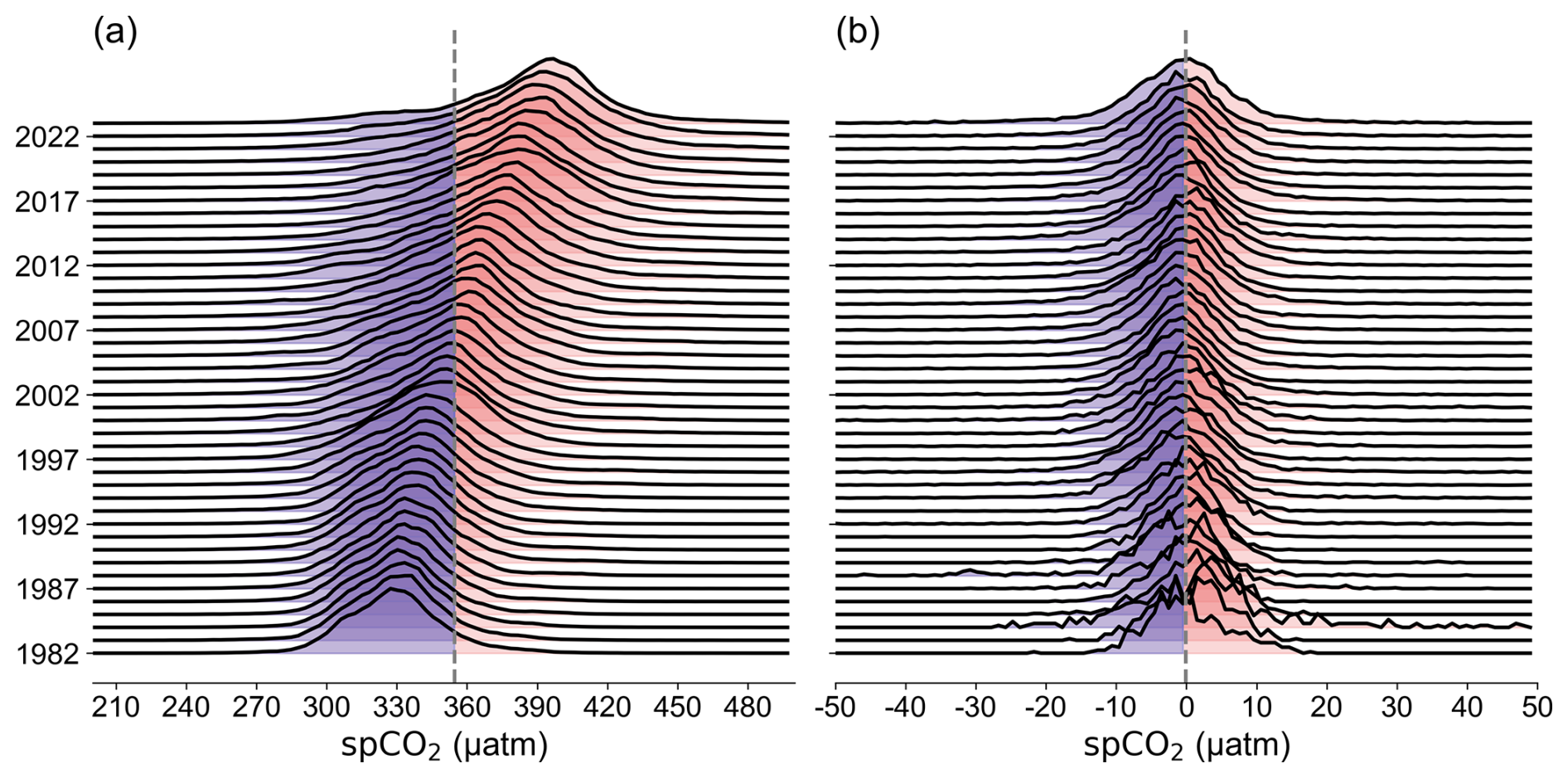
Figure 7 Probability density distributions of annual mean spCO₂ from the SJTU-AViT and bias relative to SOCAT. (a) Probability density distribution of annual mean spCO₂ from the SJTU-AViT; (b) bias probability density distribution of annual mean spCO₂ between SJTU-AViT and SOCAT. The vertical dashed line indicates the mean spCO₂ value and mean bias in panels a and b, respectively. The spCO₂ in SJTU-AViT is interpolated to match the SOCAT observation locations and times in the bias computation (see detailed computation in Sect. 2.3).

Comparison among different ocean basins (see basin boundary in Fig. S2b) indicate that spCO₂ biases in high latitude oceans, specifically the Arctic and Southern Oceans, are much larger than the biases in the low and middle latitudes of the Pacific, Atlantic, and Indian Oceans (Fig. 6). The bias of pdf line for the Arctic Ocean and Southern Ocean centers around −1.95 and −0.64 µatm, with 90 % of the biases falling within the range of −20 to +16 µatm and −14 to +12 µatm respectively (Fig. 6g and h). The biases in other ocean basins have a near-zero mean value and a narrow range of 90 % of the grid cells (−12 to +10 µatm, Fig. 6). The increased spCO₂ uncertainty in the high-latitude oceans might be related to factors such as seasonal ice cover, intense local hydrological changes, and sparse observational data. The smaller bias in the low and middle latitudes of other ocean basins can be attributed to the relatively stable oceanic conditions and the availability of abundant observational data, which help improve the accuracy of model reconstruction in regions dominated by large-scale physical processes driving air–sea CO₂ exchange. Additionally, relatively large bias observed in the tropical ocean may stem from complex interannual variability associated with climate variability like El Niño–Southern Oscillation (ENSO) and Indian Ocean dipole (IOD). Despite these regional differences, the low overall bias demonstrates the SJTU-AViT product's effectiveness in accurately capturing the spatial distribution of spCO₂ on a global scale.

The distribution of temporal evolution of annual mean spCO₂ (Fig. 7a) exhibits a clear rightward shift over time, indicating a long-term rise in spCO₂. Specifically, the annual mean spCO₂ rises from 330 to 400 µatm, with an estimated trend of 1.42 µatm yr⁻¹. This trend is consistent with the long-term increase in global oceanic spCO₂ driven by atmospheric CO₂ growth (Gruber et al., 2023; Landschützer et al., 2016), further validating the reliability of the reconstruction. In addition to this overall increase, the shape of the spCO₂ frequency distribution varies across years (Fig. 7a). Notably, the pdf gradually broadens over time, suggesting enhanced spatial heterogeneity in surface ocean CO₂ concentrations under the combined influence of rising CO₂ levels and global warming. The distribution of reconstruction biases (Fig. 7b) centers around 0 with a narrow range (<30 µatm), suggesting that the reconstruction data has no systematic offset. This further indicates that the features of shape variability across years captured by SJTU-AViT data are trustworthy. In the early years (from the 1980s to the mid-1990s), the bias distribution is more dispersed with a notable skew toward negative values, implying that the model tended to underestimate surface CO₂ partial pressure during this period. As time progresses, the bias distribution becomes increasingly concentrated and more symmetric around zero. This shift reflects improved reconstruction accuracy as the spatial coverage of observational data increased (Fig. S4). However, we note that the absolute range of biases may increase in later years. This widening is likely due to a combination of factors, including the expansion of observational coverage to regions with more extreme or marginal conditions, which introduces a larger range of reconstructed values, as well as the enhanced seasonal and interannual variability that the model may not fully capture in some regions, leading to increased biases under local or extreme conditions. Overall, the temporal evolution of the bias distribution highlights both the influence of observational coverage and the challenges in capturing high-frequency or extreme variations.

3.3 Evaluation of full spCO₂ variability and seasonal cycle

The variability in spCO₂ mainly includes the seasonal, interannual, and decadal variability. To evaluate the ability of SJTU-AViT in reproducing this variability, we compute the overall standard deviation of spCO₂ at each observational grid cell (Fig. 8a). The SJTU-AViT data product effectively reproduces the magnitude and spatial distribution of observed spCO₂ variability from 1982 to 2023, as indicated by the consistent spCO₂ standard deviation between SJTU-AViT and SOCAT data (Fig. 8a and b). The SOCAT observations (Fig. 8b) show that the strongest spCO₂ variability (SD > 30 µatm) is concentrated in the tropical Pacific Ocean, the North Pacific Ocean (40 and 60° N), the North Atlantic Ocean (40° N), and parts of the South Pacific Ocean (30° S). The SJTU-AViT successfully reproduces these spatial features, exhibiting low bias across most regions (Fig. 8d). The ratio of SJTU-AViT vs SOCAT standard deviation ranges from 0.80–1.20 which indicates the SJTU-AViT data is able to capture the 80 %–120 % varied amplitude. The bias comparison shows that the deep learning model exhibits a mean bias in standard deviation of −1.97 µatm, indicating high reliability in capturing spCO₂ variability (Fig. 8d). However, the standard deviation bias (Fig. 8d) reveals an overall underestimation of variability, with only 18.69 % of grid points showing a positive bias. This underestimation is particularly pronounced in high-latitude regions and is likely attributed to the smoothing effect of the machine learning model, which attenuates high-frequency variability, as well as the spatial inhomogeneity of observational data. In contrast, some overestimations are observed in regions with sparse data coverage, such as the Southern Ocean and the Indian Ocean (Fig. 8c).

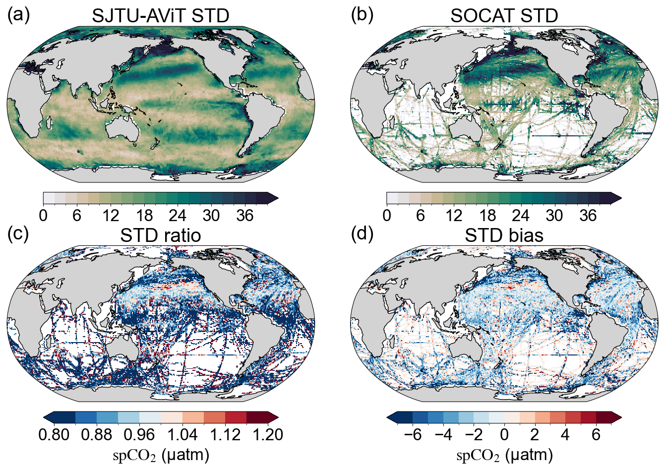
Figure 8 Comparison of spCO₂ standard deviation from 1982–2023 between SJTU-AViT and SOCAT. (a) Standard deviation of spCO₂ from the SJTU-AViT reconstruction. (b) Standard deviation of spCO₂ from SOCAT data. (c) Standard deviation ratio, representing the ratio of SJTU-AViT to SOCAT standard deviation (SJTU-AViT divided by SOCAT). (d) Standard deviation bias, showing the difference between the SJTU-AViT and SOCAT standard deviations (SJTU-AViT minus SOCAT). The standard deviation (SD) is quantified as the standard deviation of residuals after removing long-term trends. In the panels (c) and (d), the SJTU-AViT values are interpolated to match the spatial and temporal locations of SOCAT observations (see detailed computation in Sect. 2.3).

The SJTU-AViT effectively captures the large-scale seasonal distribution and amplitude of spCO₂, as shown in Figs. 9 and 10. Across the four climatological seasons – MAM (March–May), JJA (June–August), SON (September–November), and DJF (December–February) – the model reconstructs major spatial patterns that are broadly consistent with SOCAT observations. Notably, the model successfully reproduces persistently high spCO₂ concentrations in the equatorial Pacific Ocean, primarily driven by continuous upwelling of CO₂-rich subsurface waters throughout the year. It also captures elevated spCO₂ values in both the Atlantic and Pacific Oceans within the 5–30° N and 5–30° S latitudinal band during the respective summer and autumn seasons of each hemisphere, reflecting the combined effects of increased surface temperatures and seasonally weakened biological uptake. Furthermore, the model reasonably reproduces seasonal increases in spCO₂ in the North Pacific and North Atlantic (40–60° N) during Northern Hemisphere winter and early spring. This suggests that the model has likely captured underlying mechanisms, such as the deepening of the winter mixed layer and the entrainment of DIC-rich subsurface waters, which drive seasonal variations in surface ocean pCO₂ (Keppler et al., 2020). Conversely, a pronounced seasonal decrease in spCO₂ is simulated in the high-latitude Southern Ocean (south of 60° S) during the same period, indicating that the model may also have learned the influence of cooling-driven solubility changes and biological activity on ocean pCO₂. These spatial and seasonal patterns demonstrate the model's capacity to incorporate key physical and biogeochemical processes regulating spCO₂ variability.

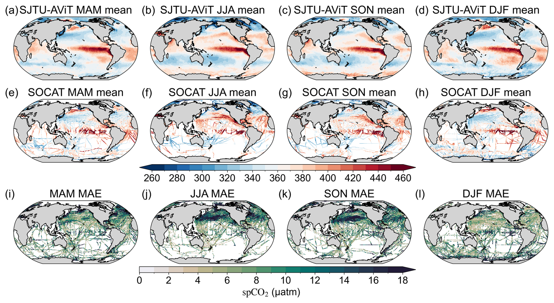
Figure 9 Comparison of seasonal spCO₂ means and mean absolute errors between SJTU-AViT and SOCAT. (a–d) Seasonal mean spCO₂ from the SJTU-AViT reconstruction for MAM (March–May), JJA (June–August), SON (September–November), and DJF (December–February). (e–h) Seasonal mean spCO₂ from SOCAT data. (i–l) Mean absolute error (MAE) of spCO₂ between SJTU-AViT and SOCAT for each season. The spCO₂ in SJTU-AViT is interpolated to match the SOCAT observation locations and times in the MAE computation (see detailed computation in Sect. 2.3).

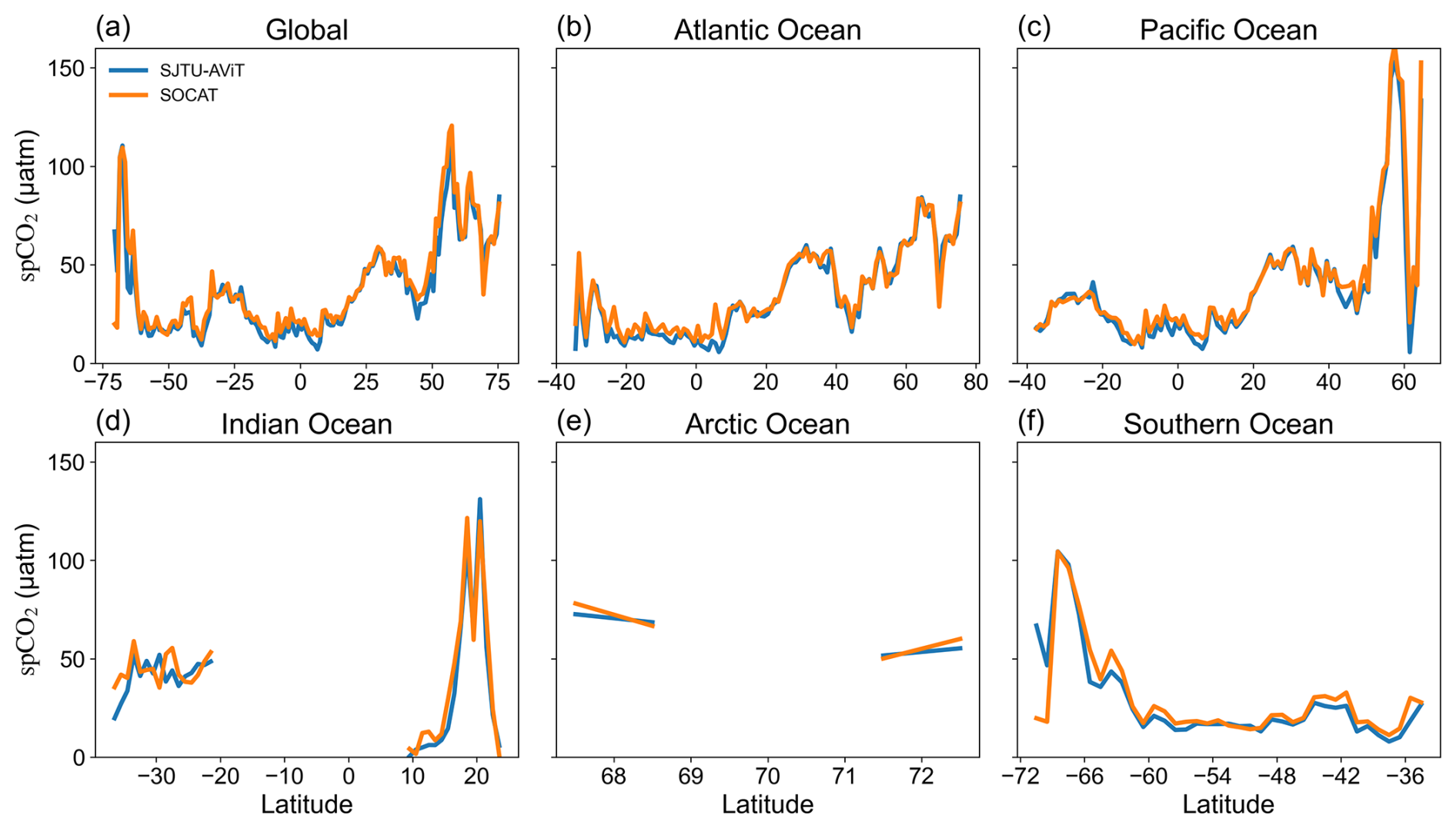
Figure 10 Comparison of meridional seasonal amplitude of spCO₂ between SJTU-AViT and SOCAT across different ocean regions from 1982–2023. The seasonal amplitude is defined as the absolute value of the difference between winter (December–February) and summer (June–August) means, subsequently averaged zonally. The spatial extents of the ocean basins are shown in Fig. S2. The spCO₂ in SJTU-AViT is interpolated to match the SOCAT observation locations and times in the comparison (see detailed computation in Sect. 2.3).

Bias analysis in Fig. 9i–l reveals seasonal model–observation discrepancies through the mean absolute error distribution. Larger errors (MAE exceeding 10 µatm) are observed in mid- to high-latitude regions during JJA and SON, particularly in the North Pacific Ocean, North Atlantic Ocean, and coastal zones. These discrepancies are likely linked to complex biological processes (e.g., seasonal blooms, net community production), which are not well captured using data-driven approaches. In contrast, lower mean absolute errors are found in subtropical gyres during DJF and MAM, with MAE values typically below 6 µatm, where variability is predominantly governed by physical drivers like SST and MLD, which are more effectively resolved by the model. Despite the pronounced interannual influence of ENSO events on spCO₂ variability in equatorial regions, the model consistently achieves low reconstruction bias across different seasons, indicating that SJTU-AViT effectively captures ENSO-related interannual anomalies in spCO₂. Additionally, the reduced observation density may contribute to the high bias of seasonal variability in the Southern Ocean and parts of the Indian Ocean.

Figure 10 further supports the model's performance in reproducing seasonal spCO₂ amplitude. Zonally averaged seasonal amplitudes across the global ocean and individual ocean basins show a high degree of agreement between SJTU-AViT and SOCAT, particularly in the Atlantic and Pacific Oceans. The model captures the amplitude peaks in the Northern Hemisphere around 40–60° N and in the Southern Hemisphere near 50° S, aligning with regions of pronounced seasonal forcing. However, deviations are observed in the Arctic Ocean, where limited data coverage likely leads to an underestimation of seasonal amplitude. Similarly, in the Southern Ocean, the model slightly overestimates seasonal amplitude in some latitudes, which may stem from the smoothing nature of machine learning algorithms and the scarcity of high-frequency, high-latitude measurements.

To evaluate the accuracy of the SJTU-AViT in capturing the seasonal phasing of spCO₂, we compared it against SOCAT climatology (Figs. S16–S18). Climatological seasonal cycles were evaluated for the global ocean and five major basins, separately for the Northern and Southern Hemispheres. The SJTU-AViT closely reproduces the timing of seasonal maxima and minima in spCO₂, generally aligning with SOCAT observations. Global maps of phase differences show that most regions deviate by less than ±1 month, with only ∼5 % of grid points exceeding this range. These results demonstrate that the reconstruction data reliably captures the observed seasonal phasing.

The bias of standard deviation in each season remains relatively low and spatially coherent across all four climatological seasons, providing further evidence of the model's robustness in representing both the magnitude and spatial distribution of seasonal spCO₂ variability (Fig. S5). Overall, the SJTU-AViT product exhibits strong skill in reconstructing seasonal spCO₂ patterns, amplitudes and phases globally. The remaining biases highlight the need for improved observational coverage in polar and biologically dynamic regions, and for enhanced model formulations that better account for nonlinear biological and physical interactions driving seasonal CO₂ variability.

3.4 Evaluation of spCO₂ variability on timescales longer than 1 year

This section evaluates spCO₂ variability on timescales longer than one year. Specifically, the variability is quantified as the standard deviation of residuals after removing both long-term trends and seasonal cycles. For the SOCAT data, calculating the residual standard deviation is challenging due to the gap in the observation record. Therefore, we use the long-term trend and seasonal amplitude derived from the SJTU-AViT data to compute the residual for the SOCAT data. While this variability encompasses both interannual and decadal variability, the signal shown here is predominantly driven by interannual fluctuations due to the limited temporal range of the data, spanning only 42 years. Therefore, for simplicity, we refer to it as interannual variability throughout this study. A comprehensive assessment of the global spatial distribution of this variability is presented in Fig. 11.

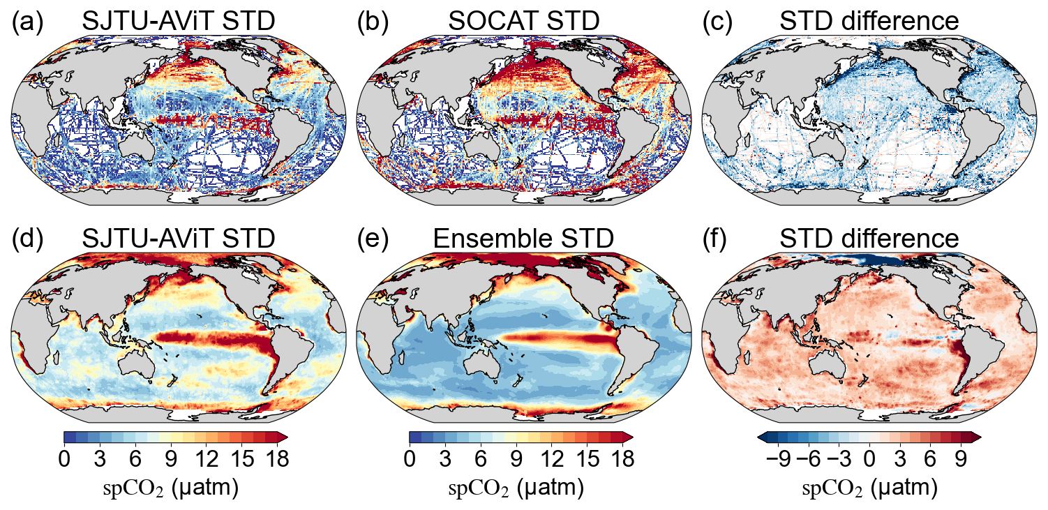
Figure 11 Comparison of spCO₂ standard deviations on timescales longer than one year between SJTU-AViT, SOCAT, and multiple data products. (a) Standard deviation of spCO₂ from the SJTU-AViT at SOCAT observation grid points. (b) Standard deviation of spCO₂ from SOCAT data. (c) Standard deviation bias between SJTU-AViT and SOCAT – panel (a) minus panel (b). (d) Standard deviation of spCO₂ from the SJTU-AViT. (e) Ensemble mean standard deviation from multiple existing spCO₂ data products. (f) Standard deviation difference between the SJTU-AViT and the ensemble mean standard deviation – panel (d) minus panel (e). The standard deviation (SD) is quantified as the standard deviation of residuals after removing both long-term trends and seasonal cycles, representing the variability on timescales longer than one year. The spCO₂ in SJTU-AViT is interpolated to match the SOCAT observation locations and times in the panel (a)–(c) comparison (see detailed computation in Sect. 2.3).

Figure 11a and b compare the interannual variability of spCO₂ derived from the SJTU-AViT model and SOCAT observations. The model accurately captures the spatial patterns of interannual variability, showing strong structural agreement with the observational dataset. High variability is well reproduced in key regions such as the equatorial Pacific Ocean (15° N–15° S, 120–280° E), the subpolar gyres of the North Pacific and North Atlantic (30–60° N), and the high latitudes of the Southern Ocean (south of 60° S). The variability in these areas is probably related to the interannual change of wind stress, upwelling, and mixed layers. To evaluate the model's performance in reproducing variability amplitude, Fig. 11c shows the bias in interannual standard deviation relative to SOCAT. On a global scale, the bias is generally small (−2.66 µatm) but tends toward slight underestimation. The most pronounced underestimations (>6 µatm) appear in the high-latitude North Pacific, North Atlantic, and Southern Ocean, where high-frequency variability is often suppressed by machine learning models due to their inherent smoothing.

Figure 11d presents the interannual standard deviation from SJTU-AViT, while Fig. 11e shows the ensemble mean of standard deviation in each existing spCO₂ products as a reference. Notably, SJTU-AViT reveals stronger variability in most global oceans – especially the Southern Ocean, tropical Pacific, and North Atlantic subtropical gyre (Figs. 11f and S6). Considering the SJTU-AViT still underestimates the interannual variability compared to SOCAT, the Fig. 11 comparison suggests the ViT-based model better retains ocean–climate variability signals rather than excessively smoothing them. The improved performance of SJTU-AViT in capturing interannual amplitude is likely due to the multi-head self-attention mechanism, high representational capacity, and the transfer learning approach applied using CMIP6 and ocean-driven biogeochemical model results. This helps the model better capture the interaction between ocean pCO₂ and interannual variability modes, leading to more accurate estimations of spCO₂ fluctuations on the interannual timescale.

We further assessed the performance of the SJTU-AViT product in the equatorial Pacific Ocean, where interannual variability of spCO₂ is the strongest in the global ocean. The SJTU-AViT dataset demonstrates clear and spatially coherent spCO₂ anomaly patterns associated with ENSO events (Figs. 12 and S7). In terms of spatial distribution, SJTU-AViT reproduces a significant decline in spCO₂ over the eastern Pacific Ocean during El Niño and a pronounced increase during La Niña. These strong comparisons between different phases of ENSO are consistent with well-established physical-biogeochemical mechanisms of ENSO-driven carbon variability through changes in upwelling, SST, precipitation, and biology (Liao et al., 2020; Sun et al., 2025). Due to the limited availability of long-term observational data, we compare the SJTU-AViT with the composite mean of multiple available spCO₂ data products. The spatial patterns of anomalies in SJTU-AViT are broadly consistent with those in the multi-model ensemble. Notably, the SJTU-AViT provides finer spatial detail, particularly in the nearshore eastern Pacific Ocean, where sharp gradients and coastal processes are more pronounced.

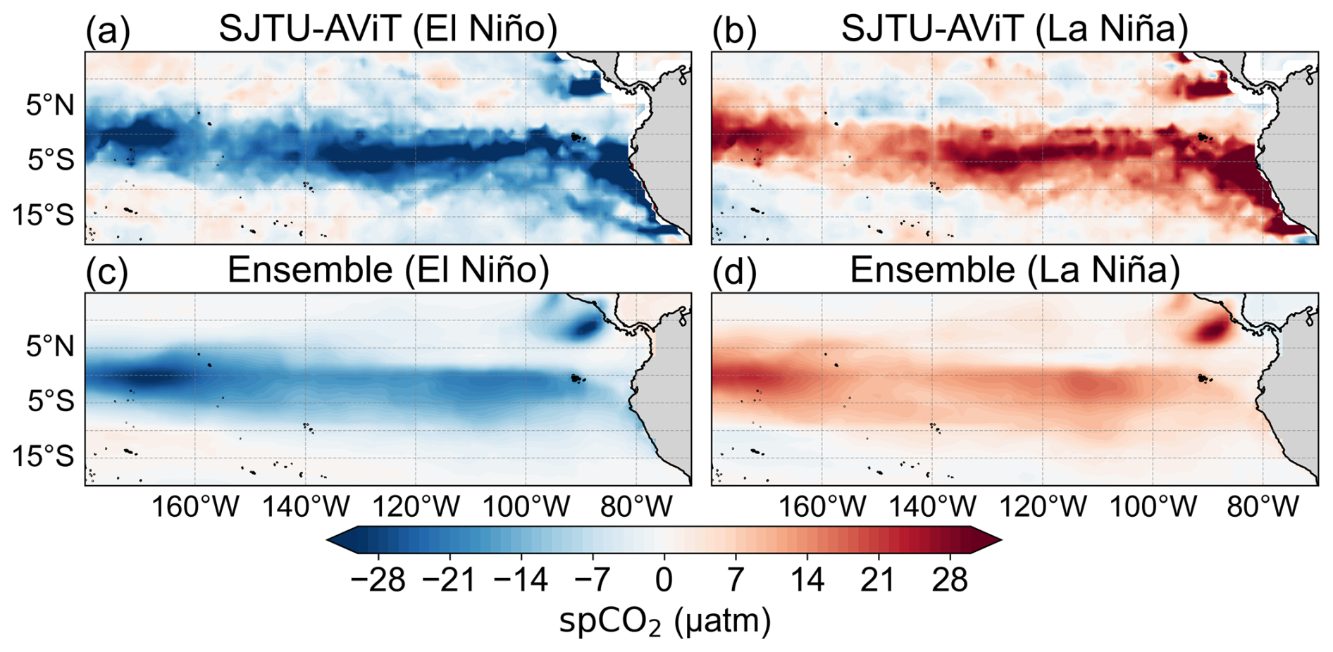
Figure 12 Comparison of spCO₂ anomalies during El Niño and La Niña events between SJTU-AViT and multiple data products. Panels (a) and (b) show the composite mean spCO₂ anomalies during eight El Niño and seven La Niña events, respectively, as reconstructed by the SJTU-AViT product. Panels (c) and (d) display the corresponding composite mean anomalies from the ensemble mean of eight spCO₂ data products. The eight El Niños and seven La Niñas are indicated in Sects. S2 and S3. The spCO₂ anomalies are defined as residuals after removing both long-term trends and seasonal cycles.

The consistency between the SJTU-AViT product and these data products is further confirmed by the temporal correlation between spCO₂ anomalies and the Niño 3.4 SST index. The SJTU-AViT shows a correlation of −0.81 and the multiple data products range from −0.40 to −0.78 (Fig. S7), indicating that the SJTU-AViT model captures the temporal evolution of ENSO-related variability in the carbon system. The latitudinal comparison also indicates a strong agreement between SJTU-AViT results, data product, and SOCAT observations during both El Niño and La Niña periods (Fig. 13).

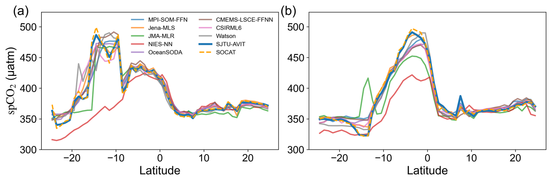
Figure 13 Comparison of meridional spCO₂ between SJTU-AViT, SOCAT, and multiple data products during (a) El Niño and (b) La Niña events. The selected El Niño events are 1997–1998 and 2002–2003, while the La Niña events are 1995–1996 and 1998–1999. These events are selected due to the availability of several cruise datasets during these periods. The cruise data are distributed over 240–280° E, which are shown in Fig. S8. The spCO₂ in all data products is interpolated to match the SOCAT observation locations and times in the comparison.

These results indicate that the SJTU-AViT model reliably reconstructs the spatial patterns of interannual and decadal spCO₂ variability at SOCAT observation sites and across the global ocean. Its ability to capture variability in line with key physical indicators such as SST and MLD demonstrates its robustness in physically consistent reconstructions. Nevertheless, regional discrepancies highlight the need for further refinement, particularly in under-observed areas and regions where non-physical factors may dominate reconstructed variability.

3.5 Evaluation of the air–sea CO₂ fluxes

The air–sea CO₂ flux based on SJTU-AViT spCO₂ reproduces consistent known features with multiple data products (Gregor et al., 2019; Landschützer et al., 2016; Takahashi et al., 2009). Elevated FCO₂ is observed along the equator, particularly in the eastern equatorial Pacific, associated with the upwelling of carbon-rich waters. In contrast, mid-to-high latitudes act as net CO₂ sinks (Fig. 14a). This substantial carbon sequestration is primarily driven by the enhanced solubility of CO₂ in cold waters, deep water mixing, transport processes, and the biological carbon pump (DeVries et al., 2017; Gregor et al., 2018; Sarmiento et al., 2004; Takahashi et al., 2009). While SJTU-AViT effectively reproduces the overall spatial patterns and mechanisms of air–sea CO₂ flux, Fig. 6 indicates that negative spCO₂ biases remain in certain high-latitude regions. The negative bias, likely associated with underrepresented high-latitude processes such as seasonal sea-ice variability and freshwater inputs, can lead to an overestimation of global ocean CO₂ uptake through the bulk equation and should be considered when interpreting the absolute flux magnitude.

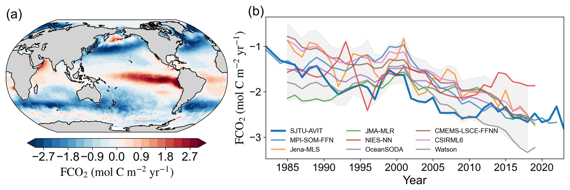
Figure 14 Spatial and temporal characteristics of air–sea CO₂ flux (FCO₂, mol C m⁻² yr⁻¹); (a) spatial distribution of the long-term annual mean FCO₂; (b) comparison of time series of yearly global integrated CO₂ flux between SJTU-AViT and multiple data products. Colored lines represent individual products, with SJTU-AViT highlighted in bold. The shaded area indicates the ±2 SD (standard deviation) range, centered on the ensemble mean. Negative = ocean uptake (sink), Positive = release to the atmosphere (source).

The time series of global air–sea CO₂ flux (Fig. 14b) shows a strengthening oceanic carbon sink over the past four decades, from −1.40 Pg C yr⁻¹ in the early 1980s to −2.60 Pg C yr⁻¹ in the 2010s. Notably, the SJTU-AViT reconstruction is consistently maintained within the ±2 SD (standard deviation) envelope of existing multi-product ensemble estimates and exhibits strong agreement with other FCO₂ products. Interannual and decadal variability are evident, such as a temporary weakening of the sink from the late 1990s to the early 21st century, reflecting the modulation of global carbon sink strength by external forcing and climate variability (DeVries, 2022; McKinley et al., 2020). In particular, the significant weakening of the carbon sink during the 1997–1998 strong El Niño event is effectively reproduced, without exhibiting the abrupt discontinuities or artificial jumps.

3.6 Evaluation of the uncertainty of reconstructed spCO₂

The global uncertainty associated with the reconstructed spCO₂ is estimated to evaluate the reliability of the data product. The estimated global mean uncertainty is 11.05 µatm, with the dominant contribution arising from the algorithm uncertainty (u_algorithm), which reaches 7.39 µatm. This value was obtained through error propagation and reflects the cumulative impact of both systematic and random errors introduced throughout the reconstruction procedure. Given the conservative nature of our uncertainty estimation, this magnitude is considered reasonable. Specifically, to ensure a conservative approach, the observational uncertainty (u_obs) for each SOCAT data point was uniformly set to 5 µatm, following established practices. The gridding process applied to SOCAT data (u_grid) resulted in an uncertainty of 6.34 µatm. The contribution from uncertainties in the input variables (u_inputs) is comparatively minor, also estimated at 1.50 µatm.

Regionally, the estimated uncertainties of reconstructed spCO₂ exhibit moderate spatial variability across the major ocean basins. Among the five RECCAP2-defined open ocean regions, the Indian Ocean shows the lowest mean uncertainty at 8.62 µatm, followed by the Pacific Ocean (10.10 µatm) and the Atlantic Ocean (10.28 µatm). Higher uncertainty levels are observed in the Southern Ocean (11.64 µatm) and the Arctic Ocean (12.45 µatm), consistent with sparser observational coverage, enhanced seasonal variability, and more complex air–sea interactions in these regions. These regional patterns suggest that while the global uncertainty level remains controlled, localized differences – particularly in high-latitude oceans – should be considered when interpreting the product in regional carbon budget assessments.

4 Discussion

In this study, we present a new reconstructed data product of spCO₂ (SJTU-AViT) with improved interannual variability using the ViT-based deep learning model. The ViT-based deep learning model integrates the Vision Transformer (ViT) architecture with physics-informed constraints and assimilates outputs from advanced ocean biogeochemical models, including CMIP6 models and ocean-driven biogeochemical model (MOM6-COBALT2). This integration enables a more precise extraction of the complex relationships between oceanic environmental variables and spCO₂. The SJTU-AViT product effectively captures key spatiotemporal patterns and reconstructs improved interannual spCO₂ variability.

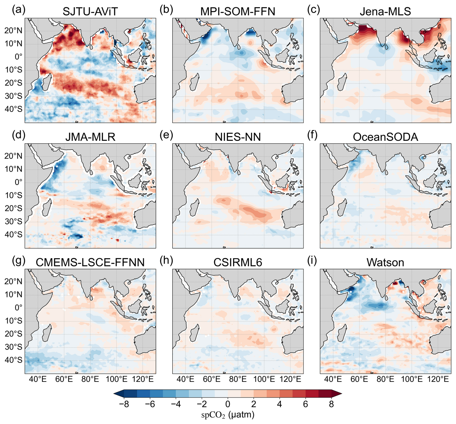
Figure 15 Spatial patterns of spCO₂ anomalies during positive IOD in the Indian Ocean between SJTU-AViT and multiple data products. The spCO₂ anomaly is the composite mean of eight positive IOD events (detailed IOD events are shown in Sects. S2 and S3). For each IOD event, the anomalies are averaged over the months of September, October, and November.

In addition, we evaluated the contributions of CMIP6 pre-training, MOM6 fine-tuning, SOCAT observations, and MOM6-derived physical-biogeochemical constraints within the SJTU-AViT framework. CMIP6 pre-training substantially improved model initialization and skill, reducing validation RMSE by ∼56.57 % versus random initialization by supplying large-scale structure and low-frequency variability. MOM6 fine-tuning further stabilized the model – especially in observation-sparse regions – lowering RMSE by ∼39.36 % and enforcing physically plausible relationships. Including SOCAT during fine-tuning was critical for local and regional accuracy, reducing RMSE by ∼72.31 % through high-quality pointwise constraints. Sensitivity tests indicate the reconstruction is largely robust to the specific choice of CMIP6 pre-training subsets, provided multiple models are used to capture diverse large-scale patterns. Finally, adding MOM6-derived physical constraints improved overall performance (MAE from 7.15 to 5.95 µatm) and reduced seasonal RMSE by 1.36 %–8.49 %, with the largest gains in high-latitude and data-sparse regions. Collectively, these results confirm that CMIP6 pre-training followed by MOM6- and SOCAT-constrained fine-tuning with physically informed constraints yields a robust, reliable, and physically consistent reconstruction of spCO₂ across spatial and temporal scales.

Despite the strong performance of SJTU-AViT, several challenges remain. A key issue is to understand and reconcile the discrepancy among different reconstruction products, particularly when considering the influence of specific climate modes such as the Indian Ocean Dipole (IOD). As illustrated in Fig. 15, during positive IOD events, nine distinct spCO₂ data products exhibit divergent composite anomaly patterns across the Indian Ocean (see IOD definition in Sect. S2). The SJTU-AViT results indicate an increase in spCO₂ in the western Indian Ocean basin and a decrease in the eastern basin (Valsala et al., 2020). The other data products present divergent or even opposite spatial patterns, raising fundamental questions about which data product most accurately reflects reality in the data-limited region. The scarcity of in situ observations in the Indian Ocean exacerbates the difficulty in determining the most reliable spCO₂ distribution (Valsala et al., 2021). These uncertainties underscore the urgent need to enhance observational efforts, particularly in regions where data products exhibit significant divergence (Rödenbeck et al., 2015). Future work should focus on expanding observation networks and leveraging autonomous platforms such as biogeochemical Argo floats (Claustre et al., 2020; Williams et al., 2017) to provide crucial validation data.

Decadal variability presents more significant challenges, with larger biases that require increased attention. Current reconstruction methods primarily capture these climate modes (e.g., Pacific Decadal Oscillation, PDO) implicitly and do not explicitly incorporate relevant indices in the machine learning model training. While increasing observational coverage is essential, it may not quickly resolve the issues related to decadal variability. A more effective solution may lie in improving the reconstruction methods themselves, particularly through the integration of physics-informed approaches. For instance, implementing physical-biogeochemical constraints, such as incorporating spCO₂ sensitivity to SST, SSS, DIC, and Alk, can significantly improve model performance, reducing the mean absolute error from 7.15 to 5.95 µatm. Future research should focus more on exploring physics-informed machine learning approaches that integrate climate indices as explicit inputs to enhance model interpretability and predictive capability (Reichstein et al., 2019; Willard et al., 2020).

While ViT-based models effectively learn spatial patterns from observational data, they remain susceptible to inherent biases in training data (Dosovitskiy et al., 2020). Systematic biases in SOCAT observations or oceanic variables (e.g., temperature and salinity) may propagate through the reconstruction process, impacting regional carbon cycle estimates (Takahashi et al., 2009). To address this, uncertainty quantification techniques such as Bayesian deep learning or ensemble learning could be incorporated to assess confidence intervals in reconstructed spCO₂ and improve anomaly detection capabilities (Gal and Ghahramani, 2016; Lakshminarayanan et al., 2016). It should be noted that the climatological MLD used in this study cannot capture interannual or monthly variability, which may slightly underestimate local or short-term impacts on spCO₂. Nevertheless, it provides adequate physical constraints for reconstructing long-term and large-scale spatiotemporal patterns. Future work will explore incorporating high-quality time-varying MLD data as it becomes available to improve model fidelity at regional and seasonal scales.

Furthermore, existing spCO₂ reconstruction approaches predominantly rely on physical environmental variables while largely neglecting biological processes. In high-productivity regions such as the North Atlantic, Southern Ocean, and Arctic Ocean, biological processes play a crucial role in regulating CO₂ exchange, with phytoplankton photosynthesis significantly lowering spCO₂ (Bates and Mathis, 2009; Boyce et al., 2010; Takahashi et al., 2009). However, Chl a only partially represents biological influences and is subject to considerable uncertainties in high-latitude regions, particularly in ice-covered areas (Arrigo et al., 2008). To better account for biological processes, future efforts should incorporate additional biogeochemical variables such as net community production (NCP) (Arrigo and Dijken, 2011; Behrenfeld et al., 2006) and phytoplankton community structure, alongside bio-optical remote sensing techniques, to enhance reconstruction accuracy and the physical coherence of carbon cycle interpretations.

The generalization capability of machine learning models is contingent on the completeness and representativeness of training data, leading to substantial uncertainties in data-sparse regions (Gloege et al., 2021). This is particularly evident in high-latitude oceans, where spCO₂ is modulated by sea ice cover, biological carbon pumps, and deep-water upwelling – processes that cannot be fully inferred from surface environmental variables alone (Mongwe et al., 2018). Since current models primarily rely on surface observations, their ability to capture vertical carbon transport and subsurface processes remains limited. Future studies should integrate three-dimensional ocean state variables (e.g., dissolved inorganic carbon and alkalinity) (Fennel et al., 2023; Wang et al., 2024; Zhou and Zhang, 2023) and incorporate physical conservation constraints (e.g., mass balance and chemical equilibrium) to enhance the physical robustness of machine learning models (Leal et al., 2020; Wang and Gupta, 2024). Additionally, applying data assimilation techniques or coupling machine learning with physics-based biogeochemical models could further improve reconstruction accuracy (Arcucci et al., 2021; Brajard et al., 2021; Chen et al., 2023).

In summary, high-resolution spCO₂ reconstruction is critical for understanding global ocean carbon sink variability. While the ViT-based approach offers an innovative solution, key challenges remain regarding dataset discrepancies, climate variability impacts, data uncertainties, and the omission of physical and biological processes. Existing reconstruction data product must be interpreted with caution when assessing regional carbon fluxes. As ocean acidification and climate change continue to alter marine carbon dynamics, improving our ability to reconstruct historical spCO₂ trends is essential for predicting the future ocean carbon uptake. Advancing spCO₂ reconstruction toward higher accuracy and reliability will require multi-source data integration, explainable machine learning, and robust uncertainty quantification techniques. Furthermore, this study highlights the critical synergy between observational programs and machine learning-based modeling approaches in achieving more precise global carbon assessments.

5 Data availability

The reconstructed spCO₂ and FCO₂ datasets are publicly available as a NetCDF file at https://doi.org/10.5281/zenodo.15331978 (Zhang et al., 2025) and will be updated regularly. The input datasets used for the reconstruction are also publicly accessible. The SST and SIC datasets were obtained from the NOAA OISST product (https://www.ncei.noaa.gov/products/optimum-interpolation-sst, last access: 20 February 2025). Chl a data were derived from the ESA CCI Ocean Colour project (https://climate.esa.int/en/projects/ocean-colour/, last access: 20 February 2025). xCO₂ data were sourced from the ESRL MBL CO₂ product (https://gml.noaa.gov/ccgg/mbl/data.php, last access: 20 February 2025). Wind speed and sea level pressure data were retrieved from the ERA5 reanalysis provided by the Medium-Range Weather Forecasts (ECMWF) (https://doi.org/10.24381/cds.f17050d7, Hersbach et al., 2023).

6 Conclusions

This study presents a novel global data product of spCO₂ reconstructed by a ViT-based deep learning model at a 1° spatial resolution for the period 1982–2023. By integrating multi-source observational data, biogeochemical ocean model results, and physics-informed constraints, the reconstructed data product demonstrates strong accuracy and spatial coherence across diverse oceanic regions, with a particular improvement in capturing interannual variability.

The model performs robustly during both the training and independent validation phases, with high accuracy (R²=0.86 in training, R²=0.82 in validation) and low bias (RMSE of 16.70 µatm in training). The implementation of physical-biogeochemical constraints can significantly improve model performance, reducing the mean absolute error from 7.15 to 5.95 µatm. The reconstructed data product shows strong agreement with SOCAT observations and accurately reproduces long-term climatological and annual mean spCO₂, with a low global mean bias of −0.21 µatm, a low mean absolute error of 5.95 µatm, and a high correlation coefficient (R=0.94). However, biases were found in coastal and high-latitude oceans, suggesting the need for further refinement in these areas.

The evaluation of seasonality reveals that the SJTU-AViT model effectively captures both seasonal patterns and amplitudes across global ocean basins, particularly in regions with stable conditions, such as subtropical gyres. On the time scale longer than one year, the model demonstrated its ability to capture higher interannual spCO₂ variability, particularly during El Niño and La Niña events, with high spatial and temporal coherence. The higher performance is likely due to the incorporation of CMIP6 model and advanced ocean biogeochemical model results during the ViT-based model training process. This approach allows the model to capture more accurate spCO₂ variability in these data-sparse regions. Additionally, it captures the global ocean carbon sink's long-term strengthening, consistent with rising atmospheric CO₂. However, uncertainties remain in high-latitude regions due to challenges in resolving complex oceanic processes. Despite this, the model's output aligns with the uncertainty ranges of existing datasets, demonstrating its reliability for global CO₂ exchange assessments.

This study highlights machine learning's potential in spCO₂ reconstruction, while identifying key challenges, such as input data limitations and model interpretability. Future work should extend this approach to higher spatial and temporal resolutions, integrate more biogeochemical parameters, and couple the model with ocean-atmosphere models for improved long-term projections. Additionally, enhancing model interpretability will be crucial for understanding the drivers of spCO₂ variability. The approach shows promise for reconstructing other carbonate system parameters, contributing to a more comprehensive global ocean carbon data product. This will support climate change research, carbon neutrality policies, and global carbon management efforts.