A global GNSS climate data record from 5085 stations spanning up to 22 years

This work presents a comprehensive global GNSS climate data record derived from 5085 stations, spanning up to a 22-year period 2000–2021. The dataset was generated using the state-of-the-art processing methodologies and precise products from the International GNSS Service (IGS) Repro-3 initiative. It includes high-quality hourly estimates of Zenith Total Delay (ZTD) and Precipitable Water Vapour (PWV), offering improved accuracy and spatiotemporal coverage. A rigorous data screening and quality assessment framework was implemented, including formal error detection, offset identification, and extensive cross-validation with ERA5 reanalysis dataset, radiosonde profiles, and Very Long Baseline Interferometry measurements. Collectively, these efforts ensured the consistency, accuracy, and homogeneity of the dataset. In addition, diurnal, monthly, and annual variations in ZTD and PWV have been analysed to evaluate and demonstrate its feasibility for monitoring climate variability, atmospheric circulation, and weather extremes. The insights provided by the dataset address critical data gaps in global climate observing systems and provide a robust foundation for advancing climate research and applications. Representing a significant milestone in GNSS climatology, this dataset serves as a vital resource for the scientific community, supporting improved understanding of atmospheric processes and more effective responses to climate-related challenges. The generated dataset is now available at: https://doi.org/10.1594/PANGAEA.982476 (Wang et al., 2025a) and https://www.gnss.studio/Login (Wang et al., 2025b).

1 Introduction

We are currently experiencing an alarming rise in global temperatures and an accelerated progression of climate change, manifesting in increasingly severe and frequent weather and climate extremes across the planet (Seneviratne et al., 2021). The repercussions of these events are profound, causing significant adverse socioeconomic consequences and posing substantial challenges to the sustainable development of human society. It is estimated that around 3.5 billion people are highly vulnerable to climate change, with over 1.5 billion already affected by weather and climate extremes (Asian Disaster Reduction Centre, 2015). Additionally, economic losses attributed to these extreme events now exceed USD 1.3 trillion annually (IPCC, 2023). Overall, the growing body of evidence on observed impacts and the escalating trend of disasters highlight a rapidly diminishing window of opportunity to enable progress towards constructing climate-resilient communities. Despite global efforts spanning several decades, considerable spatial and temporal data gaps remain in the existing climate observing networks. It is therefore important to generate long-term, homogeneous datasets for Essential Climate Variables (ECVs) to deepen our comprehension of the intrinsic nature of weather and climate extremes and enhance comprehensive climate services for the benefit of current and future generations (Bojinski et al., 2014).

Among the various atmospheric parameters, water vapour, recognised as an ECV, plays a significant role in studying global climate change and atmospheric variability (Dessler et al., 2008; Solomon et al., 2010; Labbouz et al., 2015; Ye et al., 2015). Substantial evidence also demonstrates that the dynamic movement of water vapour directly drives meteorological fluctuations (Li et al., 2023c). Consequently, access to accurate and timely water vapour data is crucial for enhancing the robustness of climate models and improving assessment of climate risks. Since the 1940s, radiosondes have been deployed to monitor atmospheric conditions and derive accurate water vapour measurements (Brettle and Galvin, 2003; Durre et al., 2006). However, these sounding balloons, typically launched twice daily from sparsely distributed stations around the globe, offer observations with limited spatiotemporal resolution (Li et al., 2003; Benjamin et al., 2004; Liu et al., 2013). In addition to radiosondes, water vapour radiometers and satellite-based instruments have been adopted to measure atmospheric water vapour content (England et al., 1993; Buehler et al., 2008). While widely adopted, these technologies face certain challenges, including high operational costs, limited temporal and vertical resolution, low precision, and susceptibility to weather conditions (Elliott, 1995; Gui et al., 2017). Given the limitations, there is a strong rationale for adopting an emerging technology, i.e., Global Navigation Satellite Systems (GNSS), for additional remote sensing of atmospheric water vapour.

Initially designed for positioning, navigation, and timing, GNSS technology, like the Global Positioning System (GPS) has broadened its applications to include atmospheric monitoring since the 1990s (Elgered et al., 1991; Bevis et al., 1992; Duan et al., 1996). In ground-based GNSS atmospheric monitoring, GNSS receivers function as atmospheric sensors by tracking changes in the arrival times of the signals as they traverse the atmosphere. Variations in water vapour, pressure, and temperature in the troposphere significantly affect the speed and trajectory of these GNSS signals, causing propagation delays. By measuring and analysing these signal delays from satellites to GNSS receivers, atmospheric parameters, like zenith total delay (ZTD) and precipitable water vapour (PWV), can be estimated (Rocken et al., 1993, 1995; Nilsson and Elgered, 2008; Wang et al., 2017). When used together with conventional techniques, the distinct advantages of GNSS atmospheric data, including high-accuracy, high spatiotemporal resolution, long-term stability, broad-coverage and all-weather capability, unequivocally enhance the potential for advancing weather and climate research and improving response to climate risks (Gradinarsky et al., 2002; Jin et al., 2007; Choy et al., 2011; Jones et al., 2020; Li et al., 2020, 2023a, b).

In recent years, the innovative utilisation of GNSS-derived ZTD and PWV estimates has spurred the development of statistical (including artificial intelligence-empowered) and numerical approaches for nowcasting and very short-range forecasting of weather extremes, such as heavy precipitation and tropical cyclones (Zhao et al., 2018, 2022; Benevides et al., 2019; Rohm et al., 2019; Manandhar et al., 2019; Zhang et al., 2022; Li et al., 2022b, c). Beyond these meteorological applications, GNSS atmospheric parameters have also significantly enriched climate studies (Hagemann et al., 2003; Bock et al., 2007; Zhao et al., 2020; Ma et al., 2021; Li et al., 2022a, d). Notably, Foster et al. (2000) demonstrated that PWV effectively captured the water vapour variability induced by the 1997–1998 El Niño event. Gradinarsky et al. (2002) reported a long-term linear increase in PWV of 0.1–0.2 mm yr⁻¹ across Scandinavia from 1993 to 2000. Nyeki et al. (2005) highlighted that GNSS-derived PWV could track all-weather water vapour trends, unlike solar precision filter radiometers (sun-photometric), which can operate only under clear-sky conditions. By contrast, microwave radiometers can retrieve PWV under cloudy and non-precipitating conditions (Westwater, 1978). Further studies of trends in PWV series were conducted in Finland and Sweden (Nilsson and Elgered, 2008) from 1996 to 2006, in Switzerland (Morland et al., 2009) from 1996 to 2007, and in South Korea (Sohn and Cho, 2010) from 2000 to 2009. Additionally, Wang et al. (2018) applied singular spectrum analysis (Wang et al., 2016a, b) to extract nonlinear trends in PWV series, demonstrating its potential for depicting the evolution of droughts and floods. Several other studies have also explored seasonal variations in GNSS atmospheric parameters, their responses to climate change, and their feasibility in monitoring climate extremes (Jin et al., 2007; Jin and Luo, 2009; Wang and Zhang, 2009; Ning et al., 2013; Jiang et al., 2017; Li et al., 2024). Collectively, these studies underscore the key role of GNSS atmospheric parameters in advancing weather and climate research.

However, despite recent advances, the potential of GNSS atmospheric monitoring remains largely under-utilised in the climate community. This is primarily due to the lack of robust long-term GNSS climate datasets, whereas climate applications typically require the use of datasets spanning several decades (e.g., 30-year climatological normal; WMO, 2007; Arguez and Vose, 2011). In this context, many datasets used in the aforementioned studies span only around 10 years, even if this is partly because the limited record length at many sites, such durations is still insufficient for uncovering the climate change signals embedded in these parameters.

Therefore, given the continuous enhancement of multi-constellation, multi-frequency GNSS capabilities, the availability of new data streams, and the extensive accumulation of GNSS data since the 1990s, this juncture presents a prime opportunity to generate a long-term, homogeneous GNSS climate dataset, thereby fully leveraging the capabilities of GNSS atmospheric monitoring for climate applications.

Numerous international academic organisations and many governmental stakeholders have embarked on initiatives to generate accurate GNSS atmospheric parameters, aiming to advance atmospheric and climate studies. For example, the Troposphere Working Group (TWG) of the International GNSS Service (IGS) exemplifies such efforts by producing the “final” tropospheric estimates. These parameters are processed by the United States Naval Observatory (USNO) utilising the “final” satellite, orbit, and Earth Orientation Parameters (EOP) combination products, typically made available around three weeks after observation (Byram et al., 2011). However, the determined ZTD time series may still exhibit inhomogeneities due to updates in reference frames and models, variations in mapping function implementations, adjustments in elevation cut-off angles, modifications to processing strategies, and changes in hardware (such as antennas and radomes). For climate-related research, maintaining the homogeneity of ZTD and PWV time series is essential, as reliable climate change monitoring relies on the utilisation of robust and consistent datasets (Vey et al., 2009; Van Malderen et al., 2014; Ning et al., 2016). Therefore, to address this, it is important to reprocess long-term historical GNSS data using consistent processing strategies, including uniform mapping functions, elevation cut-off angles, and models, like phase centre variation. In response, the IGS analysis centres have undertaken two significant reprocessing campaigns, utilising the most recent models, updated processing strategies, and the latest satellite orbits, clock corrections, and EOP estimates. The second IGS reprocessing campaign (known as “Repro-2”) produced reprocessed tropospheric parameters covering ZTD data spanning 1994 to 2013 at about 300 stations in the IGS network. Beyond IGS, other institutes, such as the Geodetic Observatory Pecný (GOP), have conducted similar efforts. GOP, for example, reprocessed GNSS data at stations in the Regional Reference Frame sub-commission for Europe Permanent Network (EPN) from 1996 (30 sites) to 2014 (300 sites) (Dousa et al., 2017), producing a combined ZTD dataset for EPN stations using data from five analysis centres (Pacione et al., 2017). From another aspect, although an enhanced integrated water vapour dataset from more than 10 000 global GNSS stations was determined in Yuan et al. (2023), the dataset is limited only to the year 2020. Therefore, while these reprocessed GNSS datasets provide valuable insights into trends and variations in water vapour, their utility is constrained by the relatively low site density and inadequate temporal coverage, necessitating further expansion and extended data acquisition endeavours.

In this work, we reprocessed historical GPS observations from over 5000 stations, spanning up to a 22-year period 2000–2021. The goal is to fulfil the requirements of climate studies for homogeneous, long-term atmospheric parameters across a broad network. This reprocessing campaign, led by the GNSS data processing for Positioning, Atmosphere, and Climate research centre (GPAC) and hereinafter referred to as “GPAC-Repro”, adopted precise satellite orbit, clock, and EOP products from the third IGS data reprocessing campaign (IGS Repro-3), in conjunction with state-of-the-art strategies and models to further ensure the quality and consistency of the dataset. The ZTD estimates derived from the GPS data were converted to PWV using temperature and pressure data from the ?fth generation of European ReAnalysis (ERA5) atmospheric reanalysis (Hersbach et al., 2020). Then, a rigorous quality assessment of the determined ZTD and PWV estimates was conducted by comparing them with their counterparts from ERA5, radiosonde, and Very Long-Baseline Interferometry (VLBI). Additionally, to elucidate the characteristics of the new dataset and facilitate its use in climate studies, we also calculated the maximum and minimum, as well as daily, monthly, and annual mean values of PWV and ZTD for each station over the entire study period. Overall, this newly reprocessed, long-term, homogeneous GNSS climate dataset is one of the most comprehensive GNSS atmospheric datasets available. It represents a significant advancement in the innovative field of GNSS climatology, providing a valuable resource for scientific communities engaged in climate studies.

2 Data and methods

2.1 Data acquisition and analysis

This reprocessing campaign initially utilised GPS observations from 5180 globally distributed stations, covering up to a 22-year period 2000–2021. The data were sourced from four archive centres, including the Crustal Dynamics Data Information System (CDDIS, ftp://gdc.cddis.eosdis.nasa.gov/gnss/data/daily, last access: 13 February 2025), the Scripps Orbit and Permanent Array Centre (SOPAC, http://garner.ucsd.edu/pub/rinex, last access: 13 February 2025), Geoscience Australia (GA, ftp://ftp.data.gnss.ga.gov.au, last access: 17 March 2025), and the Hong Kong Geodetic Survey Section of the Survey and Mapping Office (SMO, ftp://ftp.geodetic.gov.hk/rinex2, last access: 17 March 2025). The daily observations were stored in the standard Receiver INdependent EXchange (RINEX) format, which contains dual-frequency carrier phase and code measurements, typically recorded at a 30 s sampling interval. Following a rigorous data screening process, 95 sites were excluded due to identified issues with the atmospheric results, leading to a final dataset comprising 5085 stations. The detailed exclusion criteria and screening procedures are described in Sect. 3. Figure 1 illustrates the geographical distribution of the GNSS stations included in the GPAC-Repro campaign, all of which successfully passed the quality control checks. In addition to the distribution, further analysis of the data record duration and integrity across the 5085 sites is presented in Fig. 2.

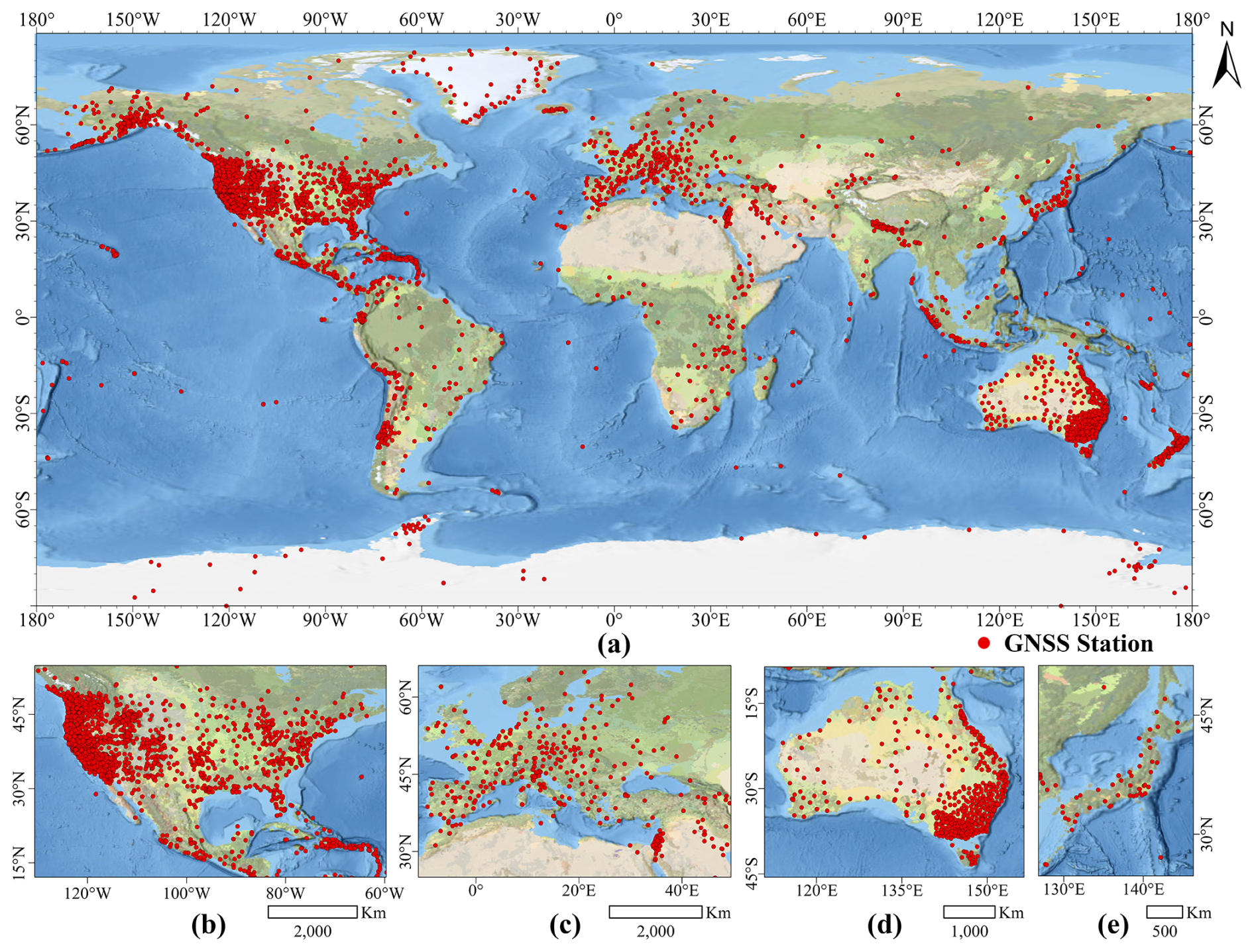
Figure 1 Geographical distribution of 5085 GNSS sites (a). Zoomed-in figures of regions with high station density, including the United States (b), Europe (c), Australia (d), and Japan (e).

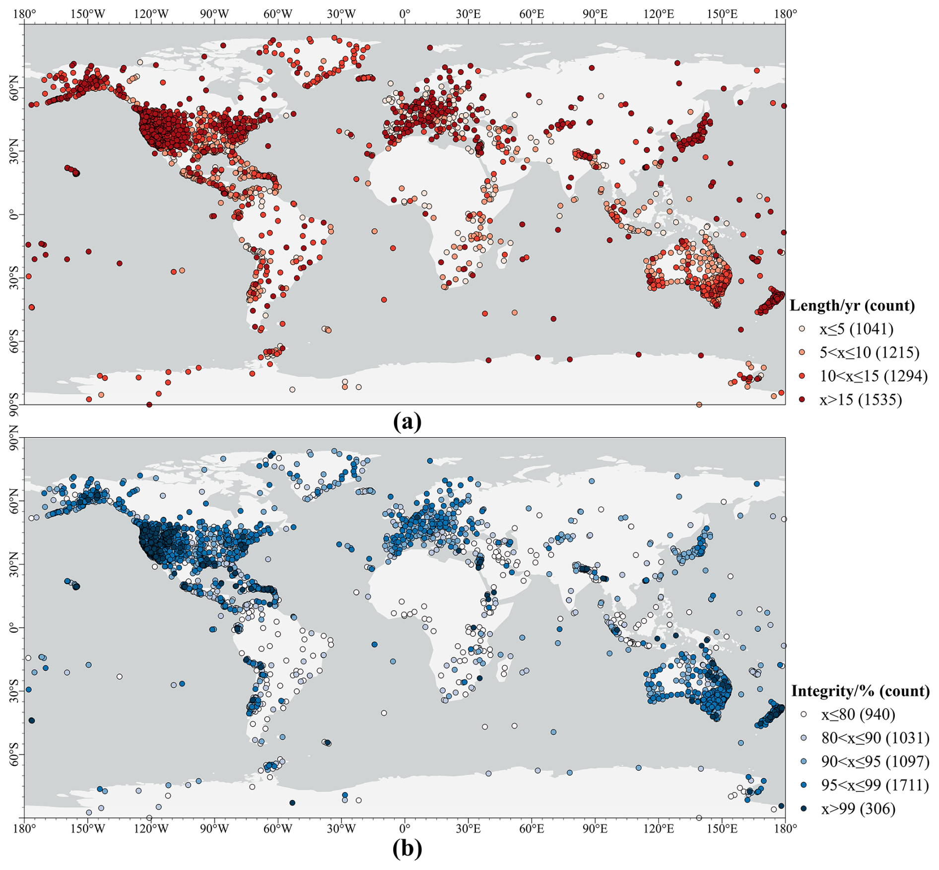
Figure 2 Recorded length (a) and data integrity (b) of the generated GNSS climate dataset across the 5085 stations.

Specifically, Fig. 2a provides an overview of the length of data records for each station, represented by colour-coded symbols. The durations range from 3 months to 22 years, offering a detailed perspective on the temporal coverage of the determined dataset. Statistically, over 30 % of the stations have records exceeding 15 years, 25.4 % and 23.9 % of the stations have records spanning 10–15 years and 5–10 years, respectively, while 20.5 % of the sites have records shorter than 5 years. Figure 2b, on the other hand, presents data integrity, with stations colour-coded based on their integrity percentage. This metric highlights the availability and continuity of the dataset across all stations, providing valuable insights into the quality of the dataset for subsequent analyses. Together, these figures emphasise the robust temporal and spatial characteristics of the generated dataset.

2.2 Data processing

This campaign adhered to the highest international standards recommended by the IGS (http://acc.igs.org/repro3/repro3.html, last access: 1 October 2024). Advanced modelling and correction techniques were implemented using Bernese GNSS Software Version 5.2 (Dach et al., 2015), incorporating the latest updates to enhance accuracy. Key updates include the International Earth Rotation and Reference Systems Service (IERS) linear pole model and the high-frequency (sub-daily) Earth Orientation Parameters (EOP) tide model. Table 1 provides a summary of the modelling features and corrections applied in the campaign.

Table 1 Modelling features and corrections adopted in the GPAC-Repro campaign.

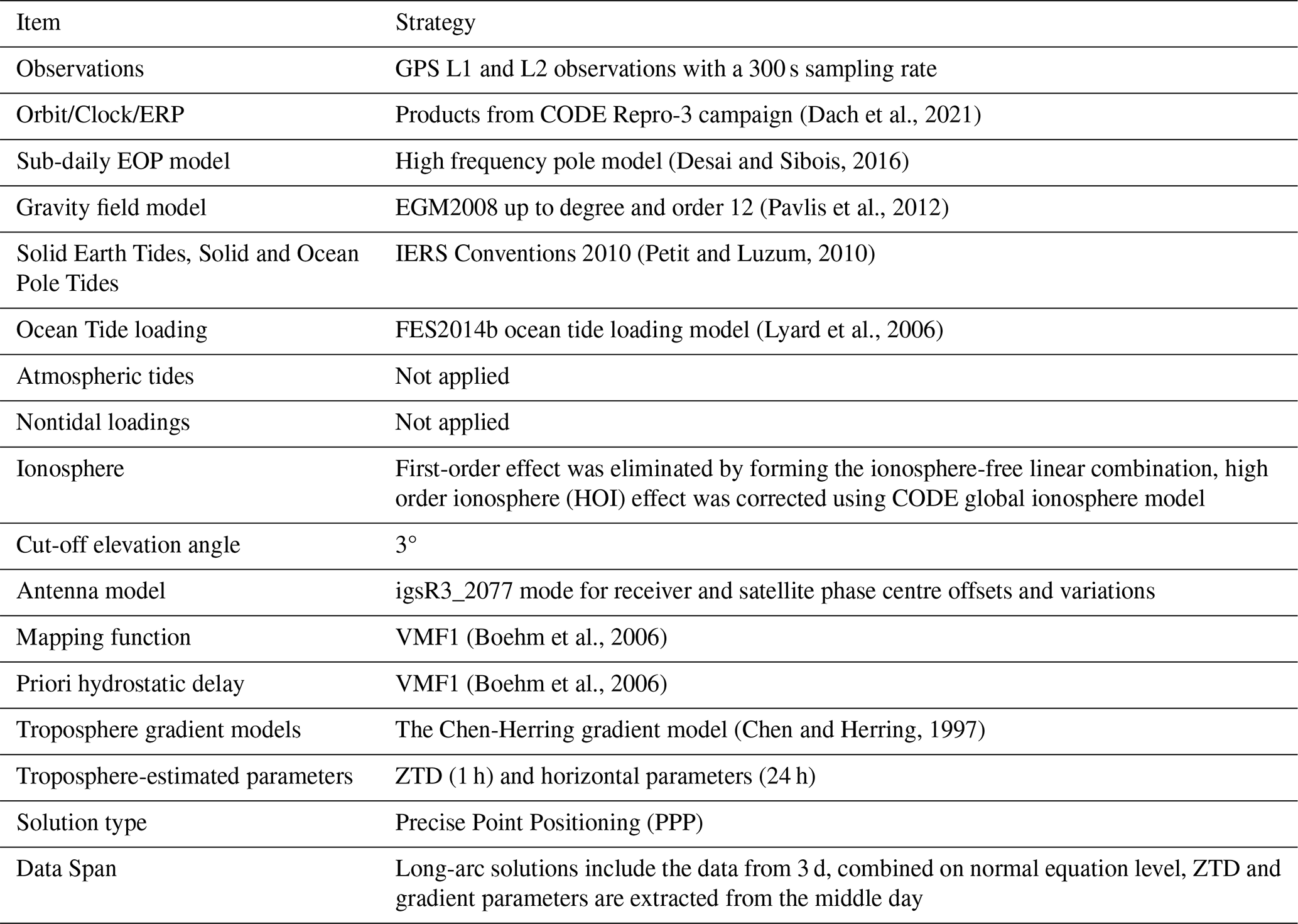
Note that, for this reprocessing effort, only GPS observations were utilised to avoid potential shifts in the ZTD series during a transition to multi-GNSS systems (Nguyen et al., 2021). Consistent with the recommendations of the IGS Repro-3, the 2010 IERS conventions were followed for modelling solid Earth tides, solid Earth pole tides, as well as ocean pole tides. Ocean tidal loading (OTL) effects were accounted for using the FES2014b model. Note that the atmospheric tidal loading (ATL) and non-tidal loading (NTL) effects were excluded due to the insufficient accuracy of current models (EPN, 2022) and their negligible impact on ZTD values (Pacione et al., 2017). According to the IERS 2010 conventions, NTL effects exhibit minimal variability over standard integration periods, and their inclusion in final solutions is generally discouraged (Petit and Luzum, 2010). Our experiments confirmed that incorporating the ATL and NTL models had an insignificant effect on ZTD estimates, yielding a mean root mean square (RMS) error of just 0.15 mm, well below typical ZTD uncertainty levels. The antenna correction model (igsR3_2077.atx) was also adopted in this work. In addition, the Vienna Mapping Function (VMF1) was used as the a priori hydrostatic delay model and mapping function, with a 3° cut-off angle. Please note that the use of a low cut-off elevation angle of 3° is based on findings from previous literature, which indicated that including low-elevation observations reduces the correlation between tropospheric parameters and station height, thereby improving the accuracy of ZTD estimates and the reliability of long-term trends (Dach et al., 2015; Dousa et al., 2017; Bai et al., 2023). Moreover, this also ensures consistency with strategy adopted by CODE in the IGS Repro-3, whose orbit, clock, and ERP products are used in our study as illustrated earlier (Dach et al., 2021). Remaining tropospheric delays, as well as horizontal gradients in the North–South and East–West directions, were estimated utilising Precise Point Positioning (PPP) mode at intervals of 1 and 24 h, respectively. One critical challenge in ZTD estimation is the day boundary problem, which occurs when GNSS data are processed independently on a daily basis (Byram et al., 2011). To address this, we adopted a 27 h time window, that comprises 24 h from the current day and an additional 3 h from the subsequent day. This is consistent with the strategy of the United States Naval Observatory (USNO) for the IGS Final Troposphere Product, which forms daily normal equations and improves the stability of tropospheric estimates near day boundaries (Byram, 2017). These equations were subsequently combined across three consecutive days to produce a 3 d solution (Dousa et al., 2017), from which ZTD estimates for the central date were extracted, thereby enhancing the continuity and accuracy of the dataset.

2.3 Retrieval of PWV

The retrieval of PWV from ZTD requires the inclusion of meteorological parameters, specifically temperature and pressure, at the locations of GNSS sites. However, the absence of meteorological sensors at most stations presents a significant challenge in obtaining these parameters. To address this and maintain consistency across the global network, this study used atmospheric data from the high-quality ERA5 dataset to provide the necessary meteorological inputs. ERA5 provides hourly atmospheric fields on 37 pressure levels at 0.25°×0.25° resolution, available from 1940 to the present (Hersbach et al., 2020).

The process begins by calculating the Zenith Wet Delay (ZWD), which is derived by subtracting the Zenith Hydrostatic Delay (ZHD) from the ZTDs obtained from GNSS data.

$$\begin{array}{}\text{(1)}& \mathrm{ZWD}=\mathrm{ZTD}-\mathrm{ZHD}\end{array}$$

The ZHD is computed using numerical integration over ERA5 pressure profiles (Haase et al., 2003):

$$\begin{array}{}\text{(2)}& \mathrm{ZHD}={\mathrm{10}}^{-\mathrm{6}}{k}_{\mathrm{1}}{R}_{\mathrm{d}}\underset{\mathrm{0}}{\overset{P_{\mathrm{ant}}}{\int }}{\displaystyle \frac{\mathrm{1}}{g\left(z\right)}}\cdot \mathrm{d}P\end{array}$$

where k₁=77.60 K hPa⁻¹ is the refractivity coefficient, R_d=287.05 J K⁻¹ kg⁻¹ represents the gas constant for dry air, and P_ant denotes the pressure at the GNSS antenna height. The local gravitational acceleration at geometric height z (in km), denoted as g(z), was determined as follows (NOAA, 1976):

$$\begin{array}{}\text{(3)}& g\left(z\right)=g_{\mathrm{s}}{\left({\displaystyle \frac{R_{\mathrm{s}}}{R_{\mathrm{s}}+z}}\right)}^{\mathrm{2}}\end{array}$$

where g_s represents the local gravitational acceleration at mean sea level at latitude φ, and R_s denotes the effective radius of the Earth at latitude φ. These parameters were determined using (WMO, 2018):

$$\begin{array}{}\text{(4)}& {\displaystyle }\begin{array}{rl}{g}_{\mathrm{s}}& \approx \mathrm{9.80620}\cdot \left(\mathrm{1}-\mathrm{0.0026442}\cdot \cos \left(\mathrm{2}\mathit{\phi }\right)\right.\\ & \left.+\mathrm{5.8}\cdot {\mathrm{10}}^{-\mathrm{6}}\cdot {\cos }^{\mathrm{2}}\left(\mathrm{2}\mathit{\phi }\right)\right)\end{array}\text{(5)}& {\displaystyle }{R}_{\mathrm{s}}=\mathrm{6378.137}/\left(\mathrm{1.006803}-\mathrm{0.006706}\cdot {\sin }^{\mathrm{2}}\left(\mathit{\phi }\right)\right).\end{array}$$

Note that the ERA5 provides 37 pressure levels ranging from 1000 to 1 hPa. Since atmospheric contributions above 1 hPa were excluded in ZHD calculations based on ERA5 profiles using Eq. (2), an additional equation was used to determined ZHD contributions above the highest pressure level of ERA5, i.e., above 1 hPa. This additional contribution was then integrated into the ZHD calculations to ensure a more comprehensive analysis (Haase et al., 2003).

$$\begin{array}{}\text{(6)}& \mathrm{\Delta }\mathrm{ZHD}\approx {\displaystyle \frac{k_{\mathrm{1}}{R}_{\mathrm{d}}{P}_{\mathrm{1}}}{g_{\mathrm{1}}}}\left\{\mathrm{1}+\mathrm{2}{\displaystyle \frac{R_{\mathrm{d}}{T}_{\mathrm{1}}}{\left(R_{\mathrm{s}}+z_{\mathrm{1}}\right)g_{\mathrm{1}}}}+\mathrm{2}{\left[{\displaystyle \frac{R_{\mathrm{d}}{T}_{\mathrm{1}}}{\left(R_s+z_{\mathrm{1}}\right)g_{\mathrm{1}}}}\right]}^{\mathrm{2}}\right\}\end{array}$$

Another important issue needs to address is that, for sites located above or below the lowest pressure level of the ERA5 dataset, interpolation or extrapolation methods were used to estimate pressure, humidity, and temperature. Details of these procedures and the conversion of GNSS altitudes (referenced to the ellipsoid) to altitudes relative to mean sea level can be found in our previous studies (Wang et al., 2016c, 2017). Once the ZWD is determined by subtracting the ERA5-derived ZHD from GNSS-derived ZTD, it is converted to PWV using the following equation (Bevis et al., 1992).

$$\begin{array}{}\text{(7)}& \mathrm{PWV}={\displaystyle \frac{{\mathrm{10}}^{\mathrm{6}}}{R_{\mathrm{w}}\cdot \left[k_{\mathrm{2}}-\frac{R_{\mathrm{d}}}{R_{\mathrm{v}}}{k}_{\mathrm{1}}+\frac{k_{\mathrm{3}}}{T_{\mathrm{m}}}\right]}}\mathrm{ZWD}\end{array}$$

where R_w=461.5 J K⁻¹ kg⁻¹ is the gas constant for water vapour, k₂=70.4 K hPa⁻¹ and $k_{\mathrm{3}}=\mathrm{3.739}\times {\mathrm{10}}^{\mathrm{5}}$ K² hPa⁻¹ are refractivity coefficients. T_m denotes the water vapour-weighted mean temperature, calculated as:

$$\begin{array}{}\text{(8)}& T_{\mathrm{m}}={\displaystyle \frac{\underset{z_{\mathrm{ant}}}{\overset{\mathrm{toa}}{\int }}\frac{P_{\mathrm{v}}}{T}{d}_z}{\underset{z_{\mathrm{ant}}}{\overset{\mathrm{toa}}{\int }}\frac{P_{\mathrm{v}}}{T^{\mathrm{2}}}{d}_z}}\end{array}$$

where z_ant and “toa” represent the height of GNSS antenna and the top of the atmosphere, respectively; P_v is the partial pressure of water vapour, and T refers to the absolute temperature. Using the aforementioned procedures, PWV values can be effectively retrieved from the determined ZTD estimates. Note that, in this study, PWV values are reported in mm, numerically equivalent to kg m⁻², i.e., 1 mm = 1 kg m⁻², for readability and consistency.

3 Data screening

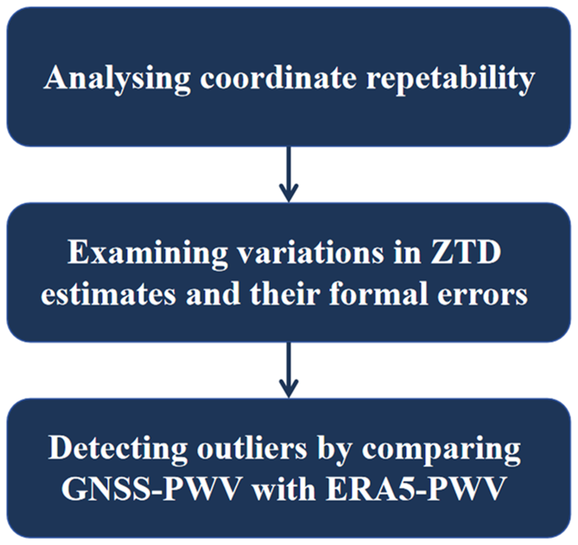
To achieve highly-quality GNSS atmospheric parameters, the adoption of the state-of-the-art processing strategies is essential. However, outliers may still occur due to observational errors or short gaps caused by equipment malfunctions or suboptimal observational conditions (Stepniak et al., 2018). Additionally, systematic biases may arise from incorrect records of receiver or antenna types. To ensure the accuracy of ZTD estimates and the resulting PWV values, a rigorous data screening procedure is indispensable for identifying and addressing problematic stations and outliers. This study introduces a comprehensive, multi-step data screening method for outlier identification. The procedure systematically analyses coordinate repeatability, examines variations in ZTD values and their formal errors, and detects outliers by comparing GNSS-PWV with reference PWV estimates from the ERA5 dataset. Figure 3 illustrates the flowchart of this multi-step data screening approach.

Figure 3 Flowchart of the multi-step data screening approach.

3.1 Screening based on coordinate repeatability

The screening process begins with an analysis of coordinate repeatability, a key indicator of the reliability of GNSS solutions. For each station, the standard deviation (SD) of daily coordinates in the North, East, and vertical directions were calculated over the entire period. Stations with an SD exceeding 100 m in any direction were excluded, resulting in the removal of 60 stations. Such large deviations were often associated with local antenna relocations or duplicate station names (Yuan et al., 2023). Next, discrepancies between daily coordinate values and corresponding weekly combined solutions were assessed. Residuals surpassing thresholds of 15 mm in the North and East directions and 30 mm in the vertical direction led to the exclusion of associated daily solutions (Dousa et al., 2017). Therefore, ZTD estimates associated with these flagged days were removed, resulting in a data reduction of 0.008 %, i.e., 34 852 hourly data samples.

3.2 Screening based on GPS-ZTD results only

Following the coordinate repeatability evaluation, ZTD values underwent further screening utilising range checks and outlier detection, following the standardised approach outlined in Bock (2020). As the first step, ZTDs outside the range of 1–3 m (Bock et al., 2014) and those with formal errors (σ_ztd) exceeding 10 mm were excluded. Please note that formal errors in the ZTD estimates are an important indicator of the quality of GNSS atmospheric parameters and are therefore widely used in screening. For context, it shows that 99.996 % of formal errors are ≤10 mm in this work. More details about the analysis of formal errors are provided in Sect. 4.1. Subsequent outlier detection was conducted for each station using thresholds determined via the Inter-Quartile Range (IQR) method based on a 15 d sliding window. Specifically, daily ZTD threshold limits were calculated using [$Q_{\mathrm{1}}-\mathrm{3}\times \mathrm{IQR}$, $Q_{\mathrm{3}}+\mathrm{3}\times \mathrm{IQR}$], where $\mathrm{IQR}=Q_{\mathrm{3}}-Q_{\mathrm{1}}$, and Q₁ and Q₃ represent the 25th and 75th percentiles, respectively, of all ZTD estimates within a 15 d sliding window centred on the target date (Yuan et al., 2023). Additionally, the upper limit for σ_ztd was determined as 2.5 times the median value, calculated over the same 15 d period. Based on these criteria, ZTDs and their formal error exceeding station-specific thresholds were flagged and removed, resulting in the removal of 0.3486 % of the ZTDs.

While this step ensures a refined ZTD dataset for PWV retrieval without requiring external reference models, e.g., ERA5, it still has several limitations, particularly in detecting inconsistencies within ZTD time series. To address this, atmospheric parameters from co-located stations were further assessed for consistency. Note that, to ensure the robustness of the analysis and minimise the influence of spatial separation, co-located stations were defined as having horizontal and vertical separations of no more than 1000 and 50 m, respectively. Additionally, each pair of co-located stations was required to have at least 8760 paired ZTD data samples, equivalent to one year of hourly observations. Given their close proximity and shared atmospheric conditions, co-located stations are expected to showcase a high level of agreement in their ZTD estimates. Figure 4 illustrates the SD and bias in ZTD at 390 co-located stations.

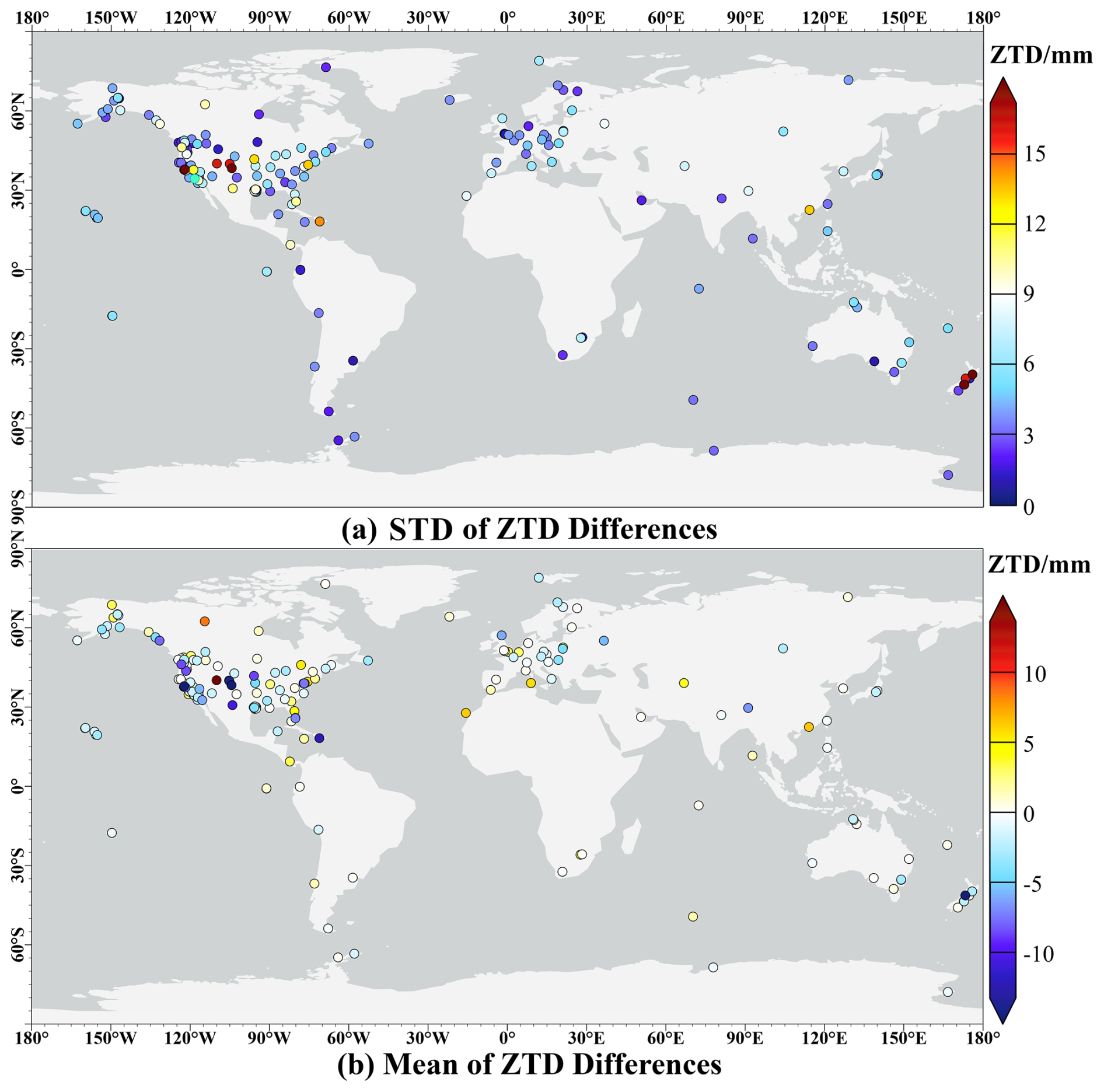
Figure 4 SD and bias in ZTD at 390 pairs of co-located GNSS stations.

It was found that the majority of station pairs (352 pairs) exhibited SD below 10 mm, with biases confined within ±5 mm, indicating strong consistency in their ZTD estimates. However, 29 pairs showed SDs ranging from 10 and 20 mm, and 9 pairs exceeded 20 mm.

After a detailed evaluation, discrepancies in ZTD between co-located GNSS sites are often attributed to height differences. It should be noted that no vertical correction was applied in this study, as the co-location comparison serves only as a preliminary step to identify potential problematic stations and to provide a general indication of the quality of ZTD estimates. In addition, in this network, 93 % of station pairs have a height difference within 10 m, corresponding to an expected ZTD difference of ∼2 mm. A vertical correction procedure may also introduce errors of comparable or larger magnitude under certain conditions like in complex atmospheric conditions or over rugged topography. Nevertheless, for local analyses where height differences are non-negligible, we recommend applying vertical corrections following methods described in Bock et al. (2022) or exploring alternative approaches. Consistent with these considerations, our dataset shows the following. As illustrated by three co-located GNSS stations in Texas, USA (30.68° N, 104.01° W) in Fig. 5, the ZTD values at MGO3, located 40 m lower than MGO2, showed a positive deviation of approximately 10 mm compared to those obtained at MGO2. In contrast, the ZTD differences between MDO1 and MGO2, with a vertical difference of 2 m, remained within ±5 mm, with an SD of 2.77 mm and a bias of 0.03 mm.

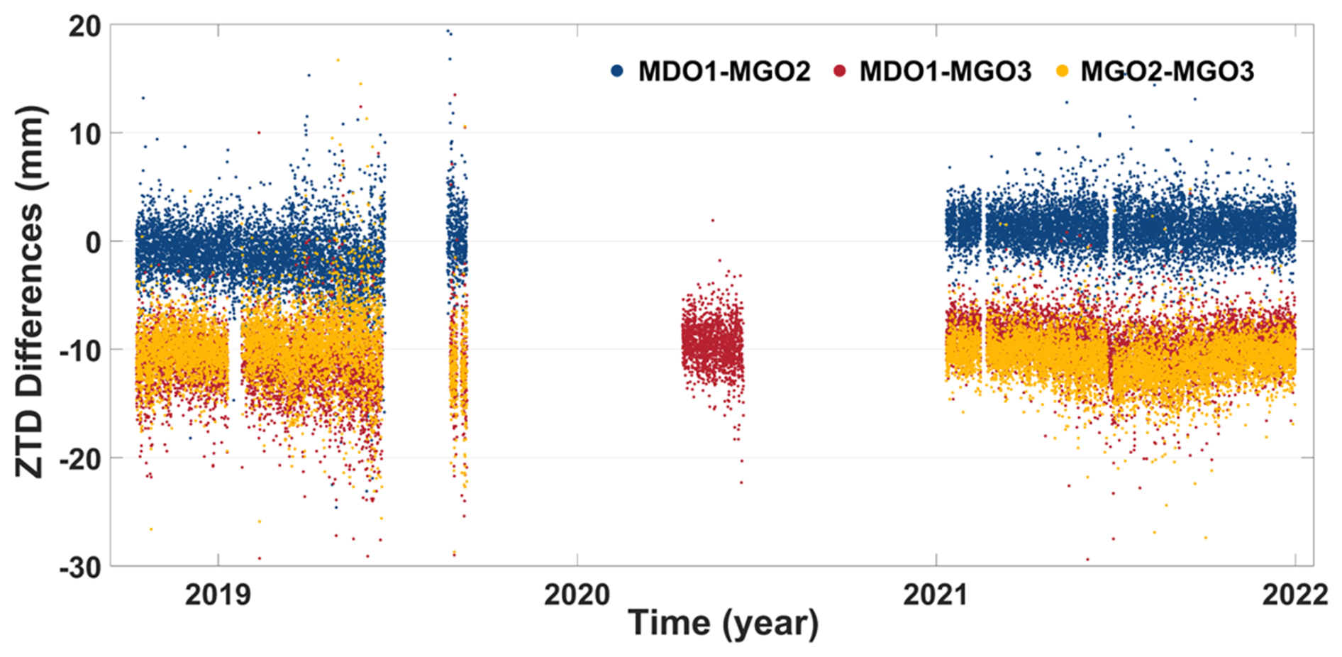
Figure 5 ZTD differences among three pairs of co-location stations in Texas, USA: MDO1–MGO2 (blue), MDO1–MGO3 (red), and MGO2–MGO3 (yellow).

Another common source of discrepancies, as mentioned before, is errors in recording receiver or antenna types, often due to human errors. As illustrated by two pairs of co-located GNSS stations, i.e., PUB1 vs. PUB2 and PUB5 vs. PUB6, in Colorado, USA (38.29° N, 104.35° W) in Fig. 6, a significant deviation with a SD of 27.42 mm was observed between the two sets of ZTD values at PUB1 and PUB2. This issue was resolved in 2008 following the replacement of PUB1 and PUB2 with PUB5 and PUB6, respectively, as part of an upgrade involving new antennas and radomes. A comparison with ERA5-derived ZTD revealed a notable positive bias of 23.1 mm at PUB2, whereas biases at PUB1, PUB5, and PUB6 were −1.8, 2.4, and 1.2 mm, respectively. Further investigation suggested that the antenna type for PUB2 was recorded as ASH700829.3 instead of the correct ASH701945E_M, leading to the overestimation of ZTD. Similar inconsistencies (biases exceeding 20 mm) were also identified at four additional stations (LRA1, UTK1, UTK2, and CLS6) when compared to co-located stations and the ERA5 dataset. The large discrepancies are likely stemmed from equipment malfunctions or suboptimal observational conditions, like strong multipath effects. In addition, equipment changes can introduce offsets, leading to inconsistencies at co-located sites and biasing long-term trend analyses by masking short-term, site-specific effects when statistics are aggregated over long periods. More details regarding the offset detection procedure adopted in our study is described in Sect. 4.3.

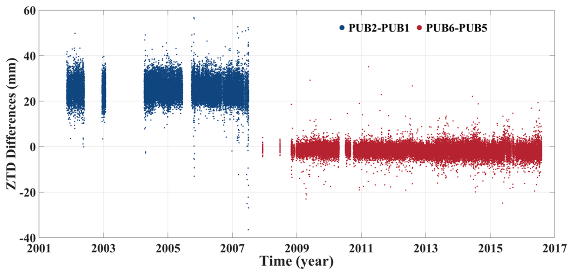
Figure 6 ZTD differences between co-location stations in Colorado, USA: PUB2–PUB1 (blue), and PUB6–PUB5 (red).

Although assessing the internal consistency of ZTD estimates from co-located GNSS sites is a valuable method for identifying potentially problematic stations, its applicability is greatly limited by the scarcity of co-located counterparts for most stations. This constraint prevents a thorough assessment across the entire network. Moreover, even when discrepancies are observed between co-located stations, accurately determining which station is problematic within the pair remains challenging without sufficient external information. Therefore, to address these limitations, additional quality control of the dataset is crucial. This can be achieved by comparing ZTD values with an independent reference dataset, such as ERA5, to validate and enhance the overall quality of the results.

3.3 Screening based on comparison with reference PWV data

In the final phase, the screened ZTD estimates were converted to PWV values and further validated using ERA5-derived PWVs as a reference. Before comparing with ERA5 dataset, we first performed an initial range check to remove unrealistic negative PWV values. The initial check excluded 0.16 % of the estimates. These outliers were predominantly observed at high-latitude and high-altitude stations, like those in Antarctica, where the average elevation is 2500 m and mean PWV values are typically below 2 mm. As highlighted in Thomas et al. (2008), remotely-sensing PWV estimates using GNSS atmospheric monitoring techniques in Antarctica is challenging. Both the dry atmospheric conditions and poor geometry of GNSS constellations, characterised by satellites visible at low elevation angles, contribute to reduced accuracy. Furthermore, the VMF1 mapping function and a priori tropospheric models are less reliable in polar regions on account of the limited availability of meteorological data (Labib et al., 2019). Additionally, uncertainties in ERA5-derived ZHD estimates can impact the accuracy of PWVs in Antarctica, where the typically low PWV levels are highly sensitive to ZHD errors.

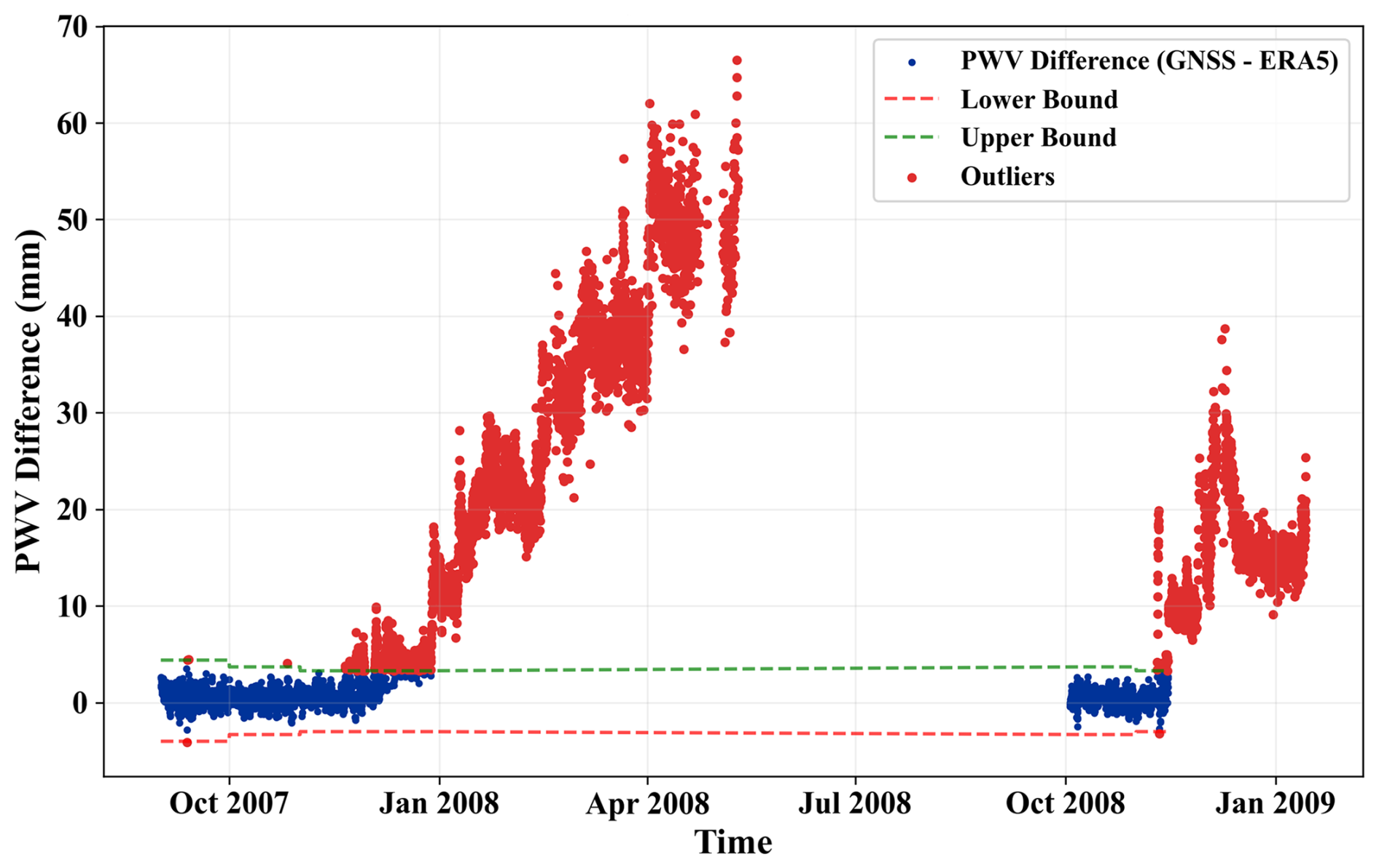
Following the removal of negative PWV values, a robust outlier detection and elimination method was applied. This method comprises two steps: (1) identifying nearby sites and (2) establishing monthly, site-specific thresholds. First, for each station, nearby stations were identified within 2° in latitude and longitude and with a vertical separation less than 500 m. Next, for the target and each nearby station, we computed the differences between the GNSS-PWVs and ERA5-PWVs. For each month, these differences were pooled to estimate the distribution and define the monthly thresholds of the target station using the aforementioned IQR-based method, i.e., [$Q_{\mathrm{1}}-\mathrm{3}\times \mathrm{IQR}$, $Q_{\mathrm{3}}+\mathrm{3}\times \mathrm{IQR}$], where $\mathrm{IQR}=Q_{\mathrm{3}}-Q_{\mathrm{1}}$, and Q₁ and Q₃ represent the 25th and 75th percentiles, respectively. The resulting monthly thresholds were then applied to the PWV time series of the target station to flag and remove outliers. This procedure was applied to all stations, yielding site-specific thresholds that account for local spatiotemporal variability, and repeated iteratively until no additional outliers were identified. This method provides more robust, locally representative thresholds than using only the PWV differences at the target station, which may fail to detect problematic results when large system inconsistencies exist, such as the PUB2 case in Sect. 3.1. To further illustrate this method, the station SNGO was analysed as an example. As shown in Fig. 7a, the nearby stations for SNGO are identified. The differences between GPS-PWVs and ERA5-PWVs at SNGO and its nearby stations were then analysed to establish monthly threshold limits, depicted as red lines in Fig. 7b. Applying these thresholds to the PWV series resulted in the identification and removal of 0.24 % of outliers (red points) that fell outside the defined range. Hence, the final screening step excluded 0.29 % of the data points, with a mean rejection rate of 0.37 % across all sites. However, it was discovered that 172 stations exhibited rejection rates exceeding 1 %. A detailed examination flagged 34 problematic sites with considerable discrepancies between GPS-PWV and ERA5-PWV, as exemplified by AC30 shown in Fig. 8. Notably, those sites flagged as “problematic” during the co-location check were also identified through this procedure, indicating the effectiveness of the ERA5 dataset as a reference for screening. After completing the rigorous multi-step data screening process, the final dataset comprises 435.65 M hourly PWV samples from 5085 sites, i.e., with 95 sites excluded as problematic and 1.09 M hourly samples removed as outliers from the initial set of 5180 stations.

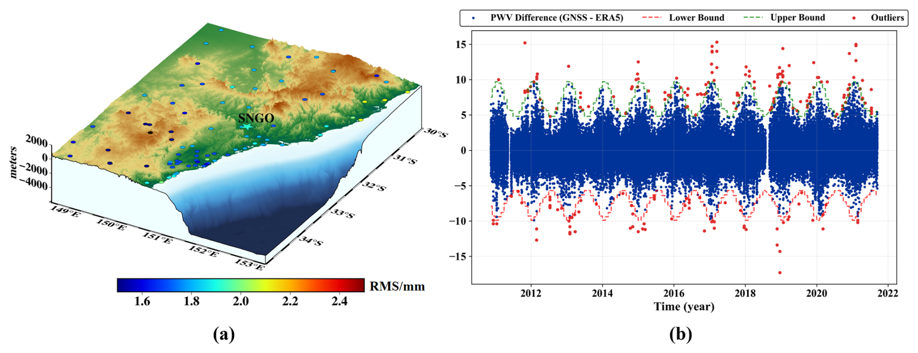
Figure 7 Identification of nearby stations for SNGO (a) and time series of PWV differences with threshold limits (b).

Figure 8 Time series of PWV differences for station AC30.

Additionally, it is crucial to note that although ERA5-derived PWV has been widely used as a reference in ZTD/PWV quality control, this practice implicitly assumes that the ERA5 dataset is sufficiently accurate, which may not always hold in all regions, especially where observational constraints are limited or atmospheric variability is high. Moreover, while we only adopt PWV for screening, we encourage ZTD-level comparisons in future analyses, as they avoid additional conversion uncertainties and potential GNSS–ERA5 representativeness differences (Jones et al., 2020). Accordingly, to accommodate various use cases, we provide two versions of the PWV dataset: an unfiltered product that contains all GNSS-derived PWV estimates after internal quality control, and an ERA5-screened product in which ERA5 is used only to flag and optionally remove gross outliers.

4 Quality assessment

4.1 Formal errors in ZTD estimations

The formal errors of the estimated ZTD are a useful indicator for analysing the quality of GNSS atmospheric parameters (Bock, 2020), as indicated in Sect. 3.2. In this regard, the distribution and cumulative percentage of formal errors across the 5085 GNSS sites employed in this study are shown in Fig. 9. The majority of formal errors range between 0.5 and 2 mm, peaking at about 1 mm. The cumulative percentage curve (red line) rises steeply, reaching 90 % at 2 mm and 99.73 % at 5 mm. The mean and median values of these errors are 1.38 and 1.23 mm, respectively. Beyond the X axis range shown in Fig. 9, as indicated in Sect. 3.2, this curve attains 99.996 % at 10 mm. Additionally, Fig. 10 depicts the annual distribution of average formal errors at 363 sites with ZTD estimates spanning 2000 to 2021. The IQRs, representing the 25th to the 75th percentiles, are depicted by blue boxes, while the median and mean values are indicated by red and black lines, respectively. The minimum and maximum values, excluding outliers (black dots, representing values greater than 1.5 times the IQR), are depicted by blue and green lines. The results indicate that most formal errors are below 4 mm, with their mean values decreasing from 2.2 mm in 2000 to 1.3 mm in 2005, stabilising thereafter. This temporal trend reflects improvements in the quality of GPS data and satellite orbit and clock products over the years. The presence of outliers (∼2 % annually) highlights occasional deviations, yet overall precision has been consistent over the two decades.

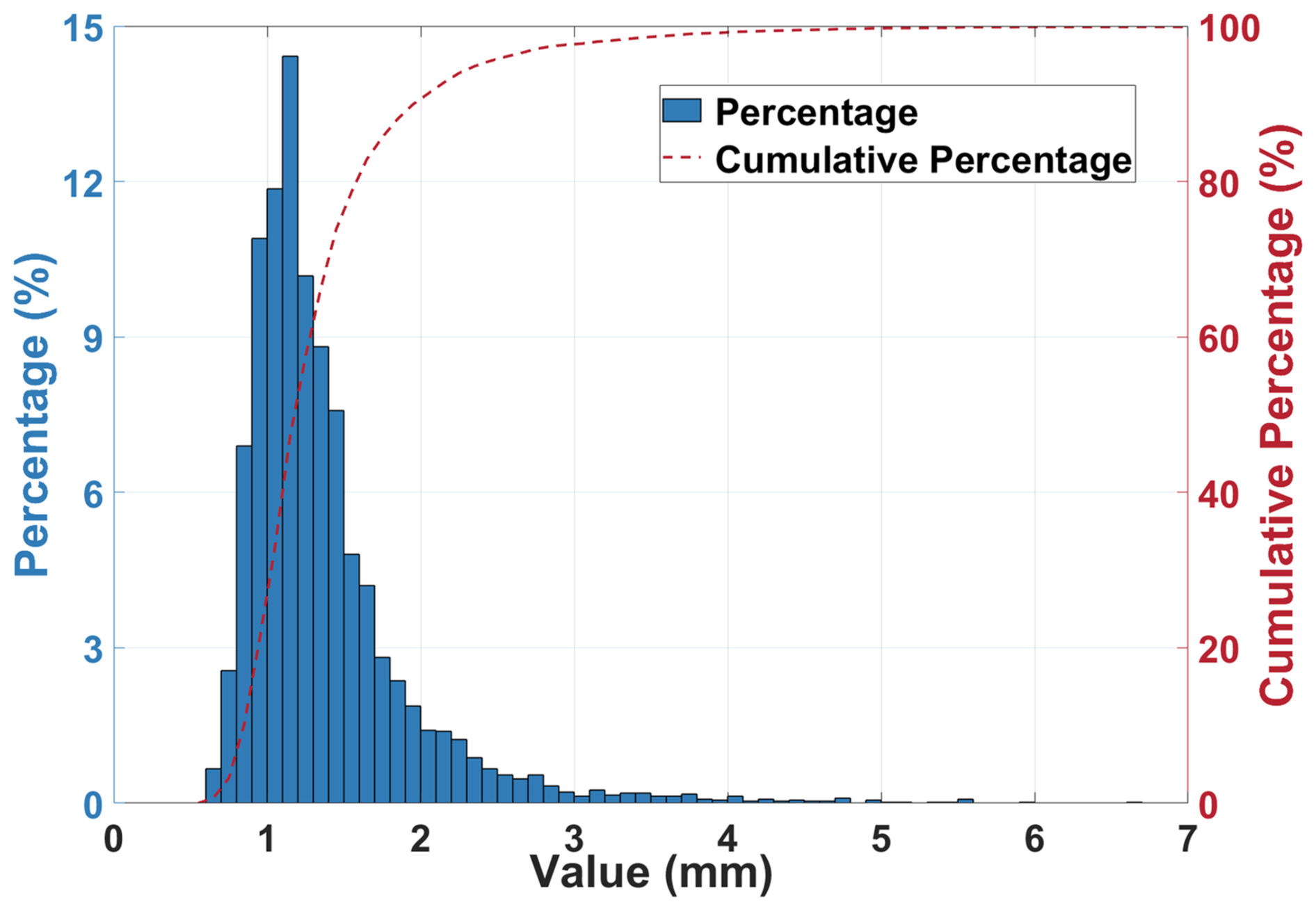
Figure 9 Distribution and cumulative percentage of formal errors across the 5085 GNSS stations.

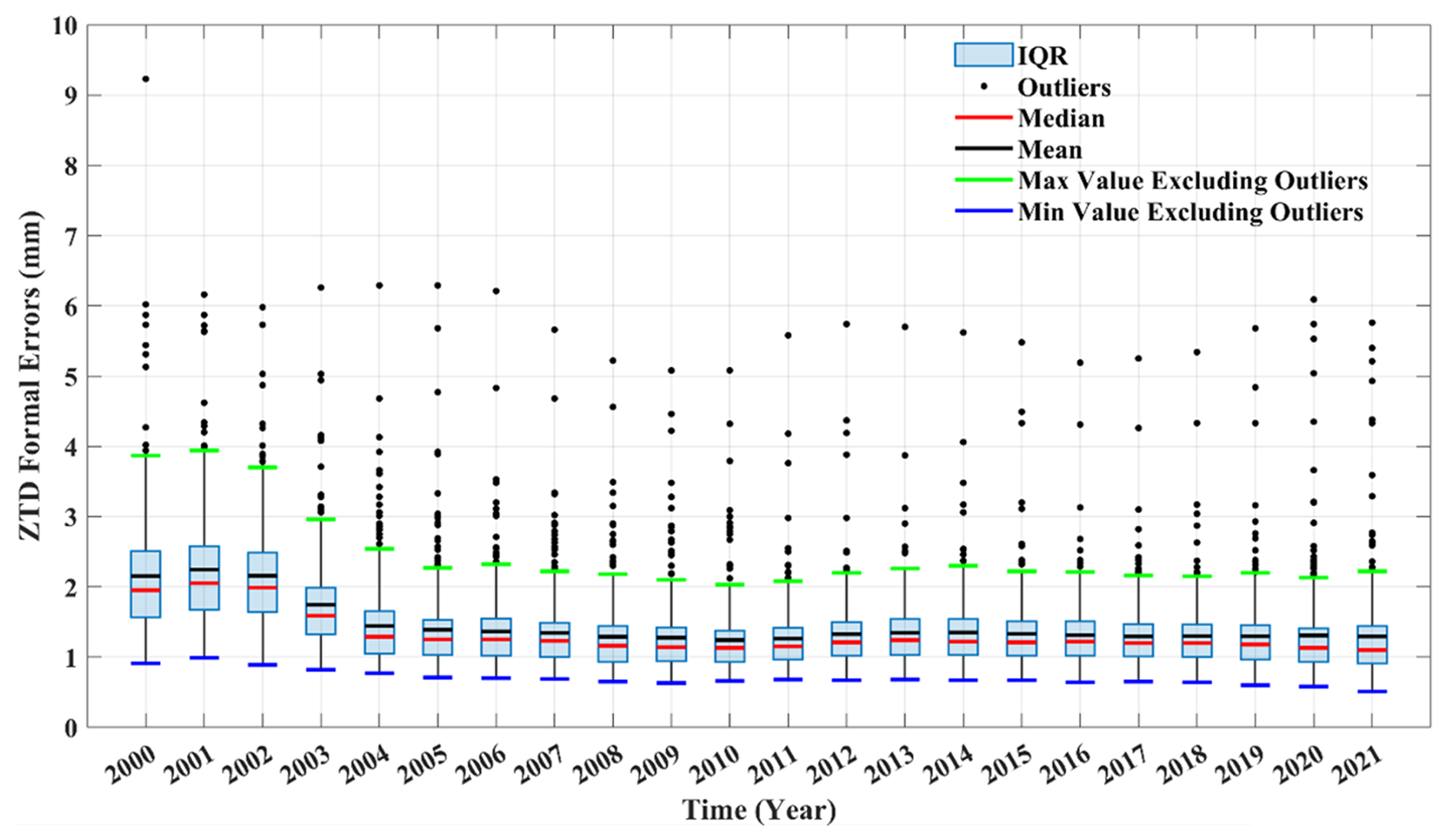
Figure 10 Annual distribution of average formal errors at 363 sites with ZTD values over the period 2000–2021.

4.2 Cross-comparison of PWV with external references

The quality of PWVs was assessed through cross-comparisons with external reference datasets. Three external data sources, the ERA5 dataset, sounding profiles and VLBI data, were adopted due to their established accuracy in atmospheric observation.

4.2.1 Comparison with the ERA5 dataset

To ensure a reliable comparison, for GNSS stations situated above or below the lowest pressure level of ERA5, horizontal interpolation and extrapolation procedures were utilised to determine pressure, humidity, and temperature at the altitude of the GNSS site based on four surrounding grid points. Detailed descriptions of these methods are available in Wang et al. (2016c, 2017). Using the pressure and specific humidity profiles at GNSS sites, PWVs were computed using:

$$\begin{array}{}\text{(9)}& \mathrm{PWV}={\displaystyle \frac{\mathrm{1}}{{\mathit{\rho }}_{\mathrm{w}}}}\underset{\mathrm{0}}{\overset{P_{\mathrm{ant}}}{\int }}{\displaystyle \frac{q}{g\left(z\right)}}\mathrm{d}P\end{array}$$

where ρ_w=1000 kg m⁻³ is the density of water vapour, P and q are the pressure (in Pa) and specific humidity, respectively. g(z) represents the local gravitational acceleration at geometric height z (in km), determined using Eqs. (3)–(5). The computed ERA5-PWVs were compared against GPS-PWVs across 4419 sites with over 1 year of continuous observations, with Fig. 11a and b illustrating SD and the mean of their differences, respectively.

Figure 11 The mean and standard deviation of differences in PWV between GPS and ERA5.

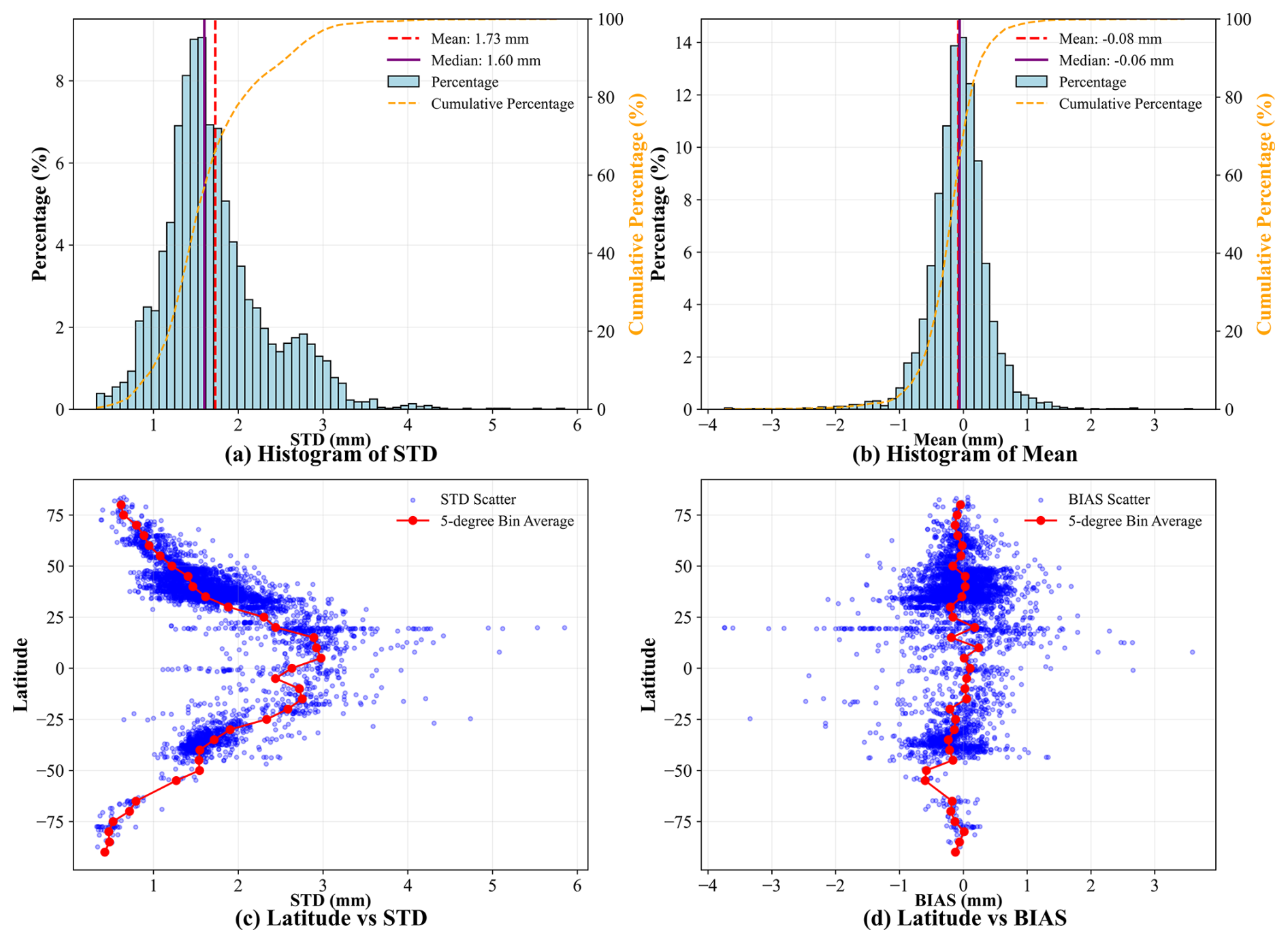
Remarkably, 96.04 % of stations exhibit SD values below 3 mm, with median and mean SDs of 1.60 and 1.73 mm, respectively. Furthermore, the mean differences at 96.33 % of the stations fall within the range of [−1, 1] mm, with a median of −0.06 mm and a mean of −0.08 mm, indicating minimal systematic bias. These results demonstrate a strong global agreement between the two datasets. Latitude-dependent discrepancies are evident, as depicted in Fig. 11c and d. The average SD, calculated within 5° latitude bins (red lines), increases from approximately 0.5 mm in polar regions to nearly 3 mm near 15° S and 15° N. This trend aligns with previous studies (Bock and Parracho, 2019; Chen et al., 2021; Yu et al., 2021) that attribute such features to the higher abundance and greater variability of water vapour in low-latitude regions compared to high latitudes. Additionally, many GNSS stations in the 15° S–15° N belt are situated on islands or coastlines, areas characterised by complex atmospheric dynamics, including high humidity and intense convection, contributing to localised anomalies in PWV values. In these areas, the accuracy of reanalysis data, which depends heavily on satellite observations, is limited in these regions due to sparse distribution of GNSS sites over open oceans and frequent cloud cover that obstructs satellite data (Lonitz and Geer, 2017). The interplay of localised atmospheric variability and observational limitations further leads to the latitude-dependent differences in PWV. Beyond latitude-related trends, regional variations are also apparent, as shown in Fig. 12. In Australia, SD increases from 1–1.5 mm in the south to 2.5–3.5 mm in the north. Similar patterns are found in the Americas, with higher SD in the east than in the west, and in Europe, where southern regions exhibit larger SD than northern areas. Additionally, ERA5-PWV tends to overestimate GPS-PWV in regions like southern Australia, Europe, eastern North America, southern Africa, southern South America, and northern Japan.

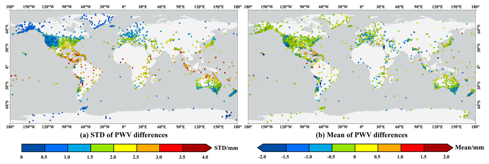
Figure 12 Regional variations of SD and mean of differences between GPS-PWV and ERA5-PWV.

Another major source of these discrepancies arises from representativeness errors inherent in ERA5, largely due to its coarse spatial resolution. These errors are particularly pronounced in areas with complex topography, like coastal and mountainous area (Bock and Parracho, 2019). ERA5-PWV was calculated as the average of atmospheric parameters from four surrounding grid points, which often misrepresents the actual atmospheric conditions at GNSS sites, especially in areas with heterogeneous terrain or coastal environments. For example, in coastal areas, ERA5-PWV averages conditions over land and sea, whereas GPS-PWV reflects measurements over land. Similarly, in mountainous areas, ERA5-PWV often fails to capture localised atmospheric conditions, such as those along slopes or in valleys, due to elevation differences and topographical complexity. These discrepancies are evident in regions like Hawaii, where elevations span from sea level to the summit of Mauna Kea (4207 m), and the Andes, with elevations ranging from valleys below sea level to peaks exceeding 6000 m. Specifically, in Hawaii, SD ranges from 1.36 to 3.64 mm, with an average of 2.75 mm, while in the Andes, SD varies from 0.65 to 4.74 mm, with an average of 2.32 mm. Stations at mountain summits typically show smaller discrepancies in comparison to those at slopes, foothills or coastal areas. This is likely due to the lower atmospheric content and reduced variability at higher altitudes, making it easier for reanalysis models like ERA5 to represent atmospheric conditions. Conversely, orographic effects in slopes and foothills induce greater atmospheric variability, complicating the ability of ERA5 to capture these nuances. Given these findings, incorporating GNSS atmospheric parameters into reanalysis models offers a promising pathway to further improving the accuracy and spatial resolution of ERA5, particularly in regions with complex topography and atmospheric variability.

4.2.2 Comparison with co-located VLBI

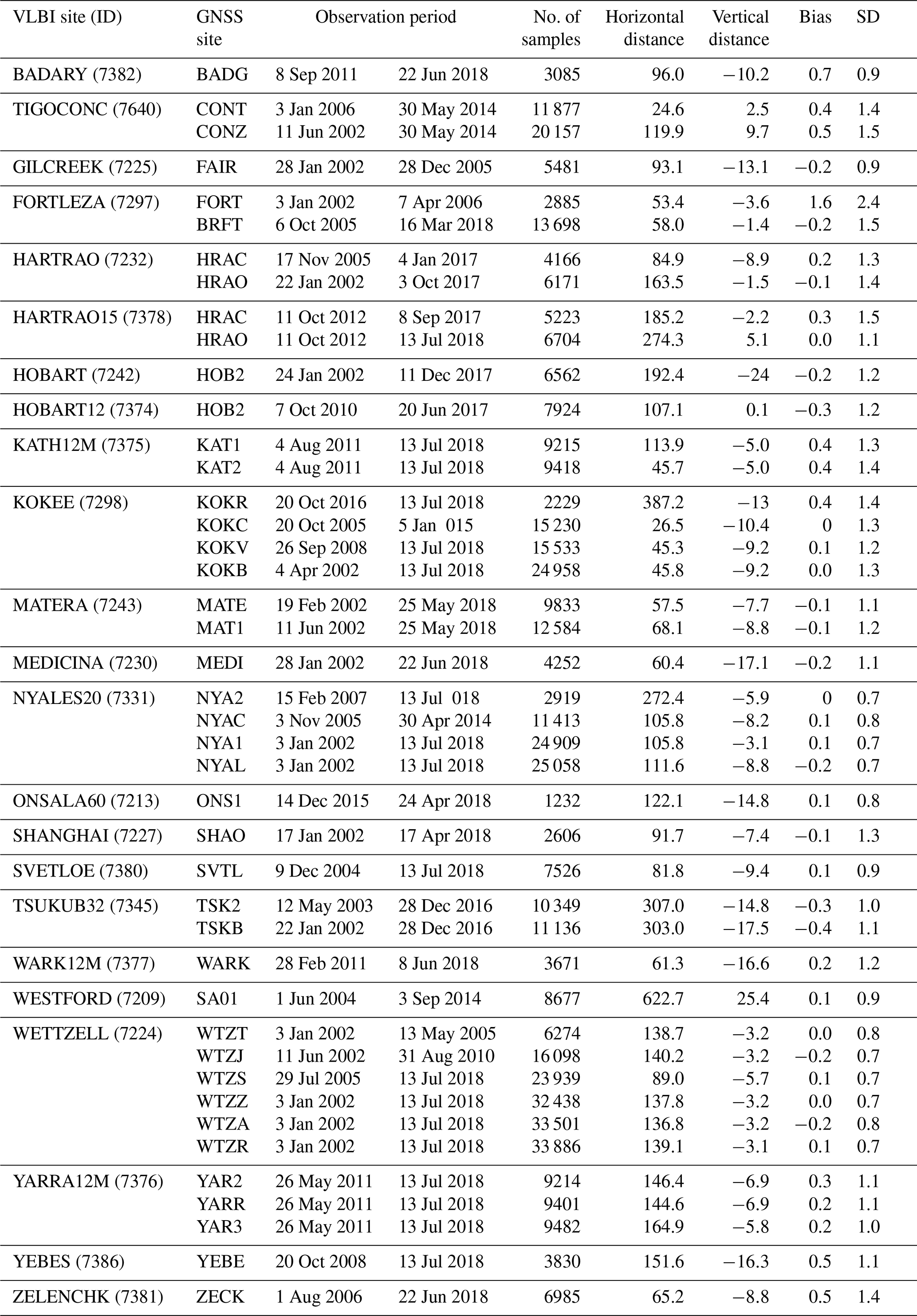
VLBI, known for its highly directive antennas, is a well-established technique for retrieving water vapour with high precision, making it a valuable tool for independently validating other techniques (Niell et al., 2001). Early comparisons of atmospheric parameters derived from GNSS and VLBI were limited in duration and geographic coverage (Ning et al., 2012). For example, Behrend et al. (2014) reported an RMS difference of 6.10 mm in ZWD estimates from VLBI and GNSS in Spain over a 9.5 h period. Choy et al. (2015) discovered a SD of 3.5 mm in PWV differences between GNSS and VLBI at Hobart, Australia. Subsequent comparisons conducted during continuous VLBI campaigns (Snajdrova et al., 2006; Teke et al., 2011, 2013; Pollet et al., 2014; Heinkelmann et al., 2016; Puente et al., 2021) showed good agreement between ZTDs from co-located GNSS and VLBI stations. Beyond these short-term campaigns, Steigenberger et al. (2007) analysed ZWD data from 24 stations over the period 1994–2004 and found SD below 10 mm at most sites. To validate the performance of the reprocessed data, PWVs were compared with those from 22 VLBI sites, using IVS-combined ZWDs and weather parameters. A total of 43 VLBI-GNSS station pairs were identified based on criteria of horizontal distances below 1 km, height differences within ±50 m, and at least 1000 paired samples. To address potential biases due to height differences between VLBI and GNSS sites, a height correction procedure was applied using atmospheric parameters at the VLBI site and ERA5-derived atmospheric data at the GNSS site:

$$\begin{array}{}\text{(10)}& \mathrm{\Delta }\mathrm{PWV}={\displaystyle \frac{\mathrm{1}}{{\mathit{\rho }}_{\mathrm{w}}}}\cdot {\displaystyle \frac{\left(q_{\mathrm{G}}+q_{\mathrm{v}}\right)}{\mathrm{2}\cdot g\left(z\right)}}\left(P_{\mathrm{G}}-P_{\mathrm{v}}\right)\end{array}$$

where P_G and P_v represent pressure at the GNSS and VLBI stations, respectively, and q_G and q_v denote specific humidity at these sites. Table 2 summarises the number of paired PWV samples, ranging from 1232 to 33 886, with an average of 11 435 per pair. Generally, PWV values from VLBI and GPS show strong agreement: 41 out of 43 stations exhibit mean differences (GPS-PWV minus VLBI-PWV) within the range of [−0.5, 0.5] mm, and 42 sites have SD values below 1.5 mm. However, the VLBI site FORTLEZA and GNSS site FORT displayed the largest deviations, with a mean difference of 1.6 mm and a SD of 2.4 mm. This notable discrepancy has been documented in earlier studies. For example, Steigenberger et al. (2007) reported a ZWD bias of 7.2 mm and an RMS of 14.1 mm, while Schuh et al. (2005) observed a bias of 13.5 mm with a SD of 9.6 mm when comparing GPS-ZTD to VLBI-ZTD at site FORTLEZA. These studies attributed the large deviations to great atmospheric variability near the equator. In contrast, the comparison between VLBI site FORTLEZA and GNSS site BRFT revealed only a minor bias of −0.2 mm and a SD of 1.5 mm. This suggests that the large discrepancy between FORTLEZA and FORT may be due to site-specific biases at station FORT, potentially caused by environmental factors or hardware issues, which warrant further investigation in future studies.

Table 2 Number of paired PWV samples at co-located GNSS and VLBI stations.

4.2.3 Comparison with radiosonde observations

Since the 1930s, radiosonde observations have provided essential insights into the distribution and variability of water vapour, establishing them as a benchmark for validating other sensing techniques. In this study, GPS-PWV was compared with their counterparts from the Integrated Global Radiosonde Archive (IGRA) Version 2 (Durre et al., 2016). Co-located GNSS and radiosonde stations were identified using criteria similar to those described earlier: (1) the horizontal distance and vertical separation must not exceed 50 km and 100 m, respectively; (2) the paired PWV series must span at least one full year with a data integrity rate of over 85 %; and (3) each date must include at least one observation during both daytime (08:00–18:00 LT, local time) and nighttime (18:00–20:00 LT); otherwise, PWV estimates from that date were excluded from the analysis. It is worth noting that we adopt a different collocation limit here than for the GNSS–GNSS and GNSS–VLBI comparisons as radiosonde-derived PWV is obtained along a balloon ascent that typically drifts tens of kilometres over 1–2 h. Imposing a very small horizontal limit would add little value for representativeness and would severely constrain coverage (e.g., with the same horizontal limit, only 22 GNSS–radiosonde pairs would remain). To balance representativeness and sampling, we therefore use a horizontal limit of 50 km. Under these criteria, we identified 402 GNSS–radiosonde pairs, with the number of paired PWV samples ranging from 888 to 23 749 (with an average of 7283 samples), equivalent to ∼10 years of observations per station. In some instances, multiple GNSS stations were co-located with a single radiosonde site, resulting in 130 unique radiosonde stations across the whole dataset, 63 of which had multiple co-located GNSS stations. A typical example is that the radiosonde station USM00072493 had 40 co-located GNSS sites using the aforementioned criteria. PWV estimates from sounding profiles were computed for comparison by interpolating or extrapolating weather parameters (pressure, temperature, humidity) to GNSS antenna height, followed by integrating specific humidity over pressure as described in Eq. (9).

As shown in Fig. 13, the comparison between the two sets of PWV revealed that the mean differences across 402 paired sites range from −4.34 to 2.50 mm, with an overall mean of −0.34 mm. The SD values of these differences vary between 0.44 and 3.86 mm, averaging 1.83 mm. Notably, 88.06 % of the sites exhibit mean differences within the range of [−1, 1] mm, and 90.80 % have SD below 3 mm, with 3 mm being a commonly used threshold for PWV accuracy in climate applications (Offiler et al., 2010), demonstrating close agreement between the two sets of PWV. According to further investigation, spatial distribution significantly influences the discrepancies. Stations in tropical regions, especially coastal and island sites, exhibit higher SD values, reflecting complex topographic and atmospheric conditions. This finding is similar to that obtained from the comparison of GPS with ERA5. In addition, analysis of the mean differences reveals distinct regional patterns. For example, GPS-PWVs tend to underestimate PWVs from sounding profiles in Australia, New Zealand, and Hong Kong (with the mean difference of −0.76 mm). In Europe, negative PWV differences predominate, while in North America, they are primarily concentrated in the east, with positive differences more common in the west. Moreover, temporal analysis of discrepancies suggests larger SD values during daytime at 81.3 % of sites, especially in tropical areas. This may stem from solar heating of radiosonde sensors, resulting in biases in relative humidity measurements. Furthermore, these day–night variations exhibit regional dependence. For example, in Europe, PWV differences are typically negative during the daytime (underestimation) but shift to positive at nighttime (overestimation). North America showed primarily negative nighttime differences, with more varied trends during the day. As per previous studies, the region-dependent differences in systematic biases are possibly attributed to diverse atmospheric conditions and differences in radiosonde sensor types.

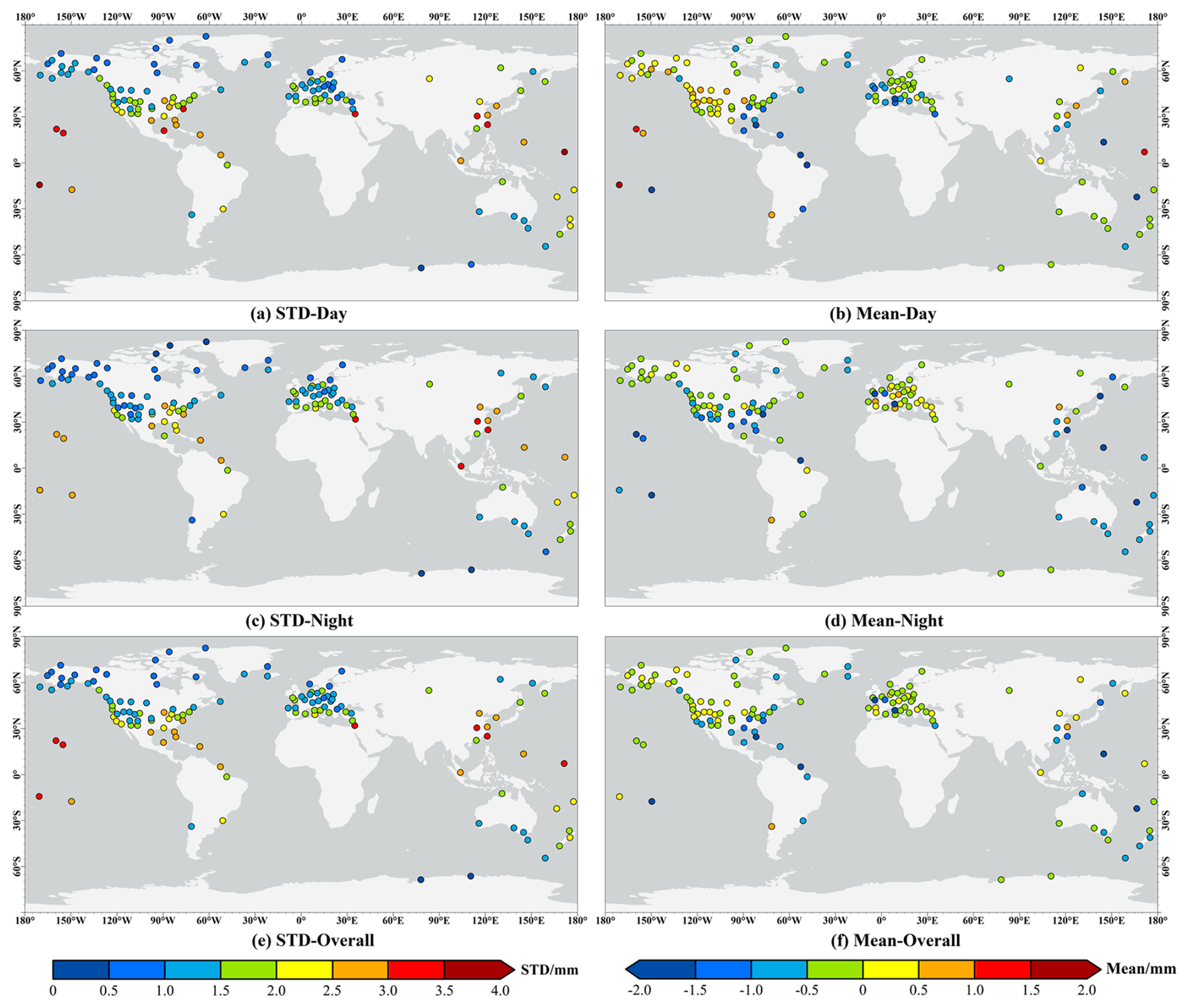
Figure 13 SD and mean differences between GPS-PWV and radiosonde-PWV.

In addition to the general analysis, eight radiosonde stations were identified, each with 10 co-located GNSS sites, providing a great opportunity to investigate the factors driving PWV differences between the two sensing techniques. For these sites, apart from the aforementioned metrics, the median, mean, and IQRs of these statistics were determined, as shown in Fig. 14.

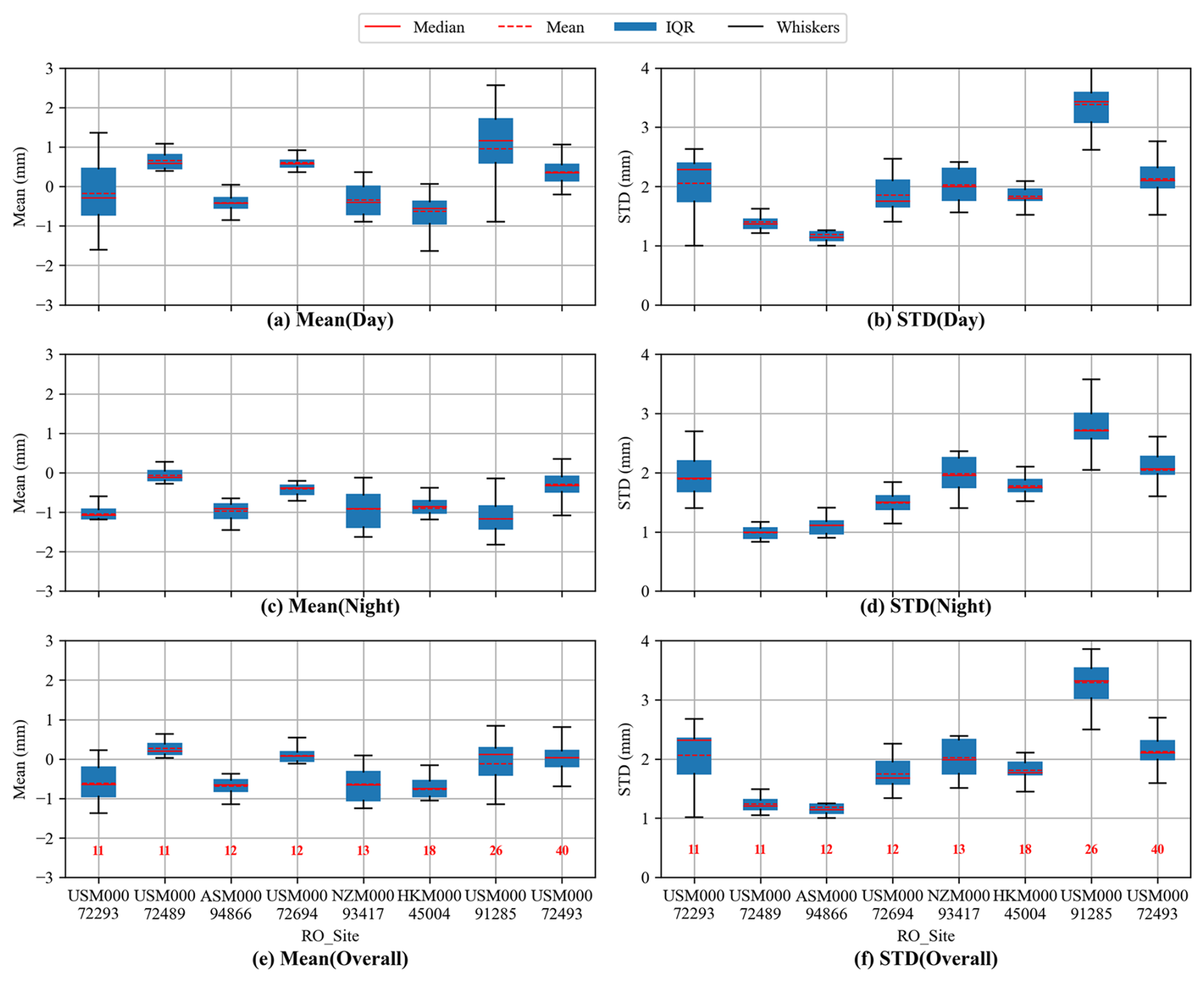
Figure 14 IQR, median, and mean values of PWV differences at 8 radiosonde and their co-located GNSS stations.

It was found that, over the entire observation period including both daytime and nighttime, five out of the eight stations exhibit IQRs below 0.5 mm, indicating strong agreement between PWVs determined from sounding data and those from multiple co-located GNSS sites. However, three sites (USM00072293, NZM00093417, and USM00091285) demonstrate IQRs exceeding 0.5 mm, mainly due to large horizontal separations (10–50 km) or significant topographic variability, as seen at USM00091285 in Hawaii. Day-night comparisons revealed generally larger IQR values during the daytime, likely attributable to diurnal PWV fluctuations or systematic biases in either radiosonde or GPS measurements.

Over the years, numerous studies have evaluated the performance of GPS-PWV using radiosonde data as a reference (Kwon et al., 2007; Pacione et al., 2011; Mo et al., 2021). Although conclusions vary across regions, our results show strong alignment with previous results and, in some cases, surpass them in performance. For example, Choy et al. (2015) reported mean SD of approximately 4 mm across six stations (2008–2012) employed in Australia, whereas this study achieved SD of 1.00–1.85 mm, with a mean of 1.03 mm. Regarding mean differences, Choy et al. (2015) found radiosonde overestimation at four of the six sites, while our findings indicate consistent radiosonde overestimation across all 24 station pairs. Park et al. (2012) analysed GPS-PWV and radiosonde-PWV in South Korea, noting a daytime dry bias in radiosonde measurements, consistent with our results for five GNSS stations co-located with the KSM00047122 radiosonde station in the same region. In polar regions, our results (mean differences ranging from −0.23 to −0.66 mm across the Arctic) align closely with Negusini et al. (2021), who reported a mean difference of −0.51 mm at the CAS1 site in Antarctica. Both studies used reprocessed products with the latest model (this study used IGS Repro3 products, while Negusini et al. (2021) used IGS Repro2 products). In Europe, our study found a mean difference of −0.29 mm and an SD of 1.4 mm across 51 station pairs over the time period 2000–2022, which compares to Pacione et al. (2017), who reported a mean difference of 0.6 mm using 183 sites over the study period 1996–2014. Both studies agree that radiosonde-ZTD (PWV) generally underestimates GPS-ZTD (PWV). Overall, despite extensive inter-comparisons, systematic errors in both GPS and radiosonde measurements continue to hinder definitive conclusions about their absolute accuracy, even for the same region and period. Variations in processing strategies, co-location criteria, as well as temporal variability (Buehler et al., 2012; Guerova et al., 2016) highlight the pressing need for standardised methodologies to ensure consistent and reproducible results across inter-comparisons.

4.3 Offset detection

Despite the fact that GNSS reprocessing eliminates changepoints caused by inconsistencies in data processing strategies, the determined PWV time series may still include offsets introduced by receiver, antenna or radome replacements, and observation environment changes. Hence, a consistency check remains necessary. To detect these offsets, this study adopted the penalised maximal t test modified for first-order autoregressive noise in time series (PMTred) method, as described in Wang et al. (2007) and Wang (2008), using the ERA5 dataset as an external reference.

A total of 2485 sites with observation periods exceeding 10 years and data missing rates below 20 % were selected. For each station, the time series of monthly mean PWV differences between GPS and ERA5 data was subjected to the PMTred test. Standardised log files for each site recorded all station-related changes. Initially, a 95 % confidence level, as the critical value (CV), was applied to identify all potential changepoints. If a detected changepoint corresponded to a recorded change within a six-month time period (before or after) in the log file, it was identified as a documented changepoint. For unrecorded changes, a stricter 99.9 % confidence level was utilised, and changepoints exceeding the threshold were also recorded (Ning et al., 2016). Based on this approach, results revealed that 1416 of the 2485 stations exhibited a total of 2427 changepoints in their PWV difference time series, while the remaining 1069 stations showed no changepoints. The detailed classification, counts, and performance of changepoints are listed in Table 3. Among these, 1190 changepoints were undocumented, potentially due to unrecorded hardware changes or environmental factors. Of the documented hardware changes, 386 were linked to receiver replacements, 137 to antenna changes, 157 to simultaneous receiver and antenna changes, and 557 to firmware upgrades.

Table 3 Classification and performance of the detected changepoints.

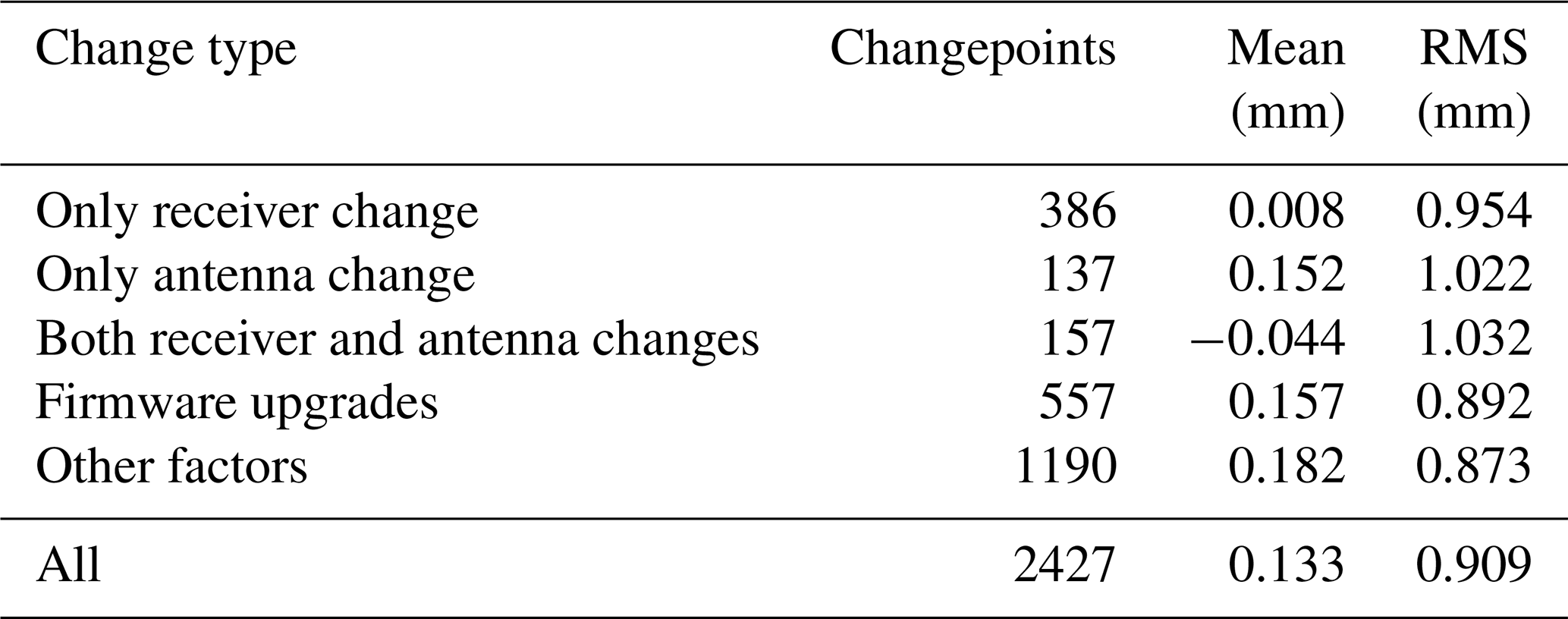
For clarity, the detected changepoints are provided as flags alongside the PWV series, and the archived PWV time series are not modified based on these detections. Although ERA5 is used as a reference to aid detection, it is not the actual “truth”, as previous studies suggest that both reanalysis and GNSS data may contain inhomogeneities (Bock and Parracho, 2019; Zhang et al., 2019; Yuan et al., 2025). Moreover, in this study, we did not perform a separate changepoint search on ZTD, ZHD or T_m. Since PWV is derived from these parameters, any discontinuity in them can induce a corresponding offset in PWV, and we will further examine these in detail in future updates. Additionally, to strengthen robustness, our future releases will also cross-compare multiple detection methods (Van Malderen et al., 2020; Quarello et al., 2022; Nguyen et al., 2025) and adopt relative-homogeneity checks based on multiple pairwise comparisons (Caussinus and Mestre, 2004; Menne and Williams, 2009; Nguyen et al., 2024).

5 Further analysis

After comprehensively illustrating the characteristics and assessing the quality of the dataset, this work further advances by offering a preliminary analysis, focusing on its innovative applications in the climate community. Specifically, the maximum, minimum, and diurnal, monthly and annual mean values of PWV and ZTD estimates are determined and analysed.

5.1 Analysis of maxima and minima of PWV and ZTD

In this study, we first identified the hourly maxima and minima of PWV and ZTD for each site over the whole period, as shown in Fig. 15. Generally, as per the statistics, PWV minima across all stations range from 0 to 43.6 mm, while maxima span 3.2 to 88.5 mm. For ZTDs, minima vary from 1.21 to 2.57 m, and maxima range from 1.32 to 2.80 m.

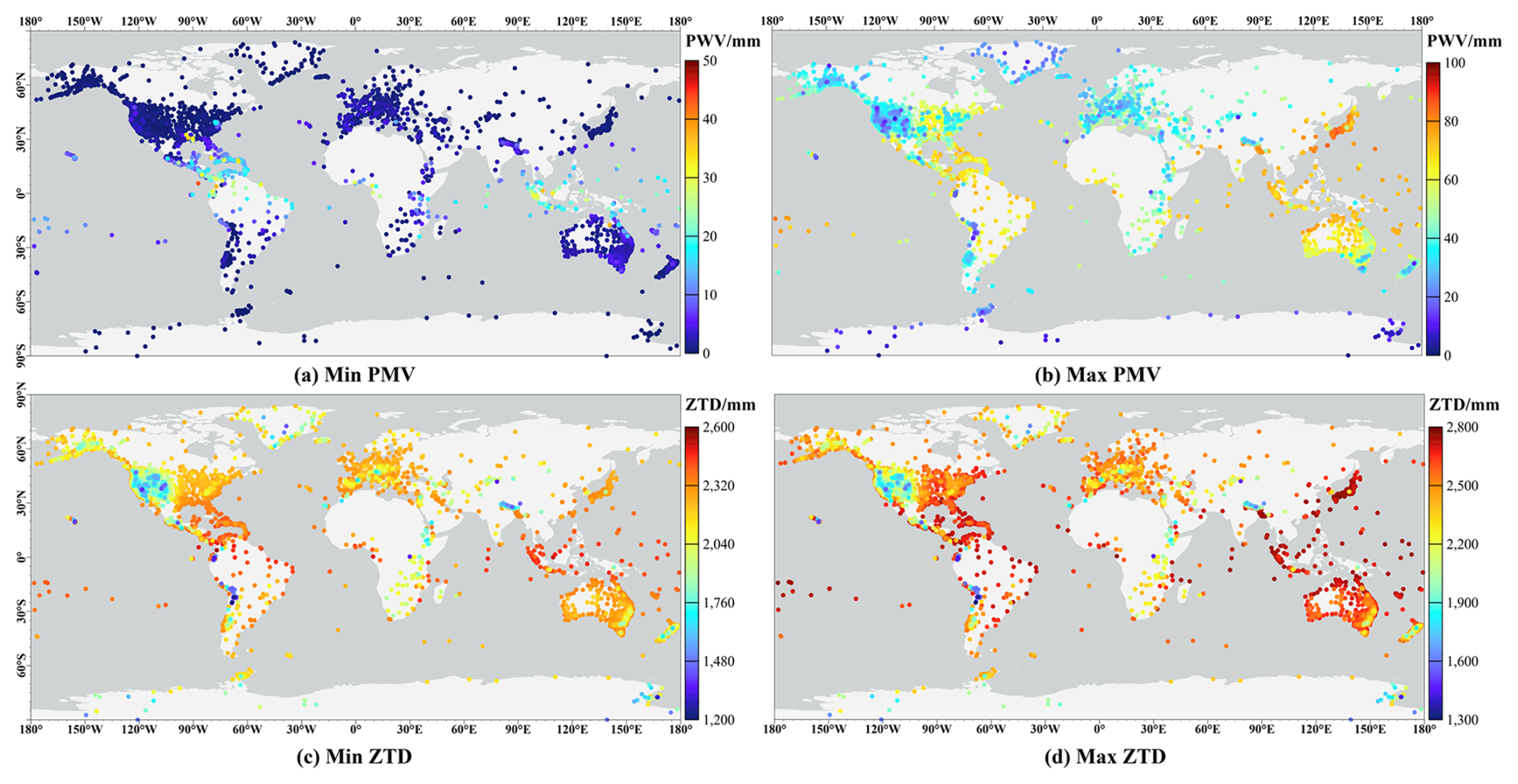
Figure 15 Maxima and minima of PWV and ZTD for each station over the whole period.

By taking a closer examination, some further insights can be revealed. Figure 15a, i.e., the PWV minima, illustrates the different patterns along latitudinal gradient. Specifically, PWV minima tend to increase toward the equator, with higher values observed in low-latitude regions (30° N–30° S) and near-zero values in mid- to high-latitude areas (30–90° N and 30–90° S). However, PWV minima exhibit no clear trend with longitude. This finding is also evident, albeit less pronounced, in Fig. 15b, which displays PWV maxima. The observed variations are influenced by factors like latitude, altitude, as well as weather and climate conditions. For example, as reported in Yuan et al. (2023), PWV maxima exhibit complex geographical patterns. The lowest PWV maximum value of 3.2 mm occurs at the AMUN station in Antarctica (89.99° S, 139.15° E), a region with persistently low temperatures and year-round ice and snow cover, which limits the capacity to hold water vapour, resulting in low PWV. Additionally, AMUN sits at an elevation of about 2816 m, where lower atmospheric pressure further decreases water vapour. In contrast, the highest PWV maximum value of 88.5 mm is recorded at the G212 station in Okinawa (26.21° N, 127.66° E), a subtropical location with a warm, humid climate affected by moist air from the Pacific Ocean. During rainy/monsoon seasons and typhoon events, this area experiences particularly higher water vapour content, which is exactly the case in this study. Furthermore, in contrast to the AMUN station, the lower elevation of the G212 station (38 m) results in higher atmospheric pressure and denser air, enabling it to retain more water vapour.

Figure 15c and d presents the minima and maxima of ZTD, which exhibit similar but distinct patterns, in comparison to Fig. 15a and b, due to the aforementioned influencing factors. Although PWV can be obtained from ZTD through a conversion factor dependent on meteorological parameters, i.e., temperature, this factor varies by station. In other words, although a typical station presents a direct relationship between ZTD and PWV, the global characteristics of ZTD and PWV maxima and minima differ significantly. For example, the lowest PWV values occur at different stations, however, the lowest ZTD maximum and minimum both appear at the LLST station in the Andes Mountains (25.17° S, 68.52° W) at an altitude of 5272 m. This high elevation leads to reduced atmospheric pressure and, consequently, lower ZTD values. Moreover, the dry air at high altitudes decreases the wet delay, an important component of ZTD, compounded by thinner atmospheric layers and fewer air molecules, which also contribute to lower ZTD values.

In general, the geographical characteristics of the maxima and minima of PWV and ZTD are affected by factors including latitude, altitude, and regional meteorological and climate conditions. Hence, when applying the parameters in weather and climate research, careful consideration of these factors is essential for accurate analysis and interpretation.

5.2 Analysis of diurnal and monthly mean PWV and ZTD

Although hourly PWV and ZTD values are widely utilised in various atmospheric and meteorological research, expanding the applicability of the dataset, especially for climate research, which depends on parameters reflecting long-term atmospheric conditions, require additional processing. In this study, the daily and monthly mean values of PWV and ZTD were calculated to facilitate comprehensive, long-term assessments. To minimise the impact of missing data on the analysis, we applied a strict inclusion criterion: Daily means were computed only when at least 21 hourly estimates were available, i.e., corresponding to at least 87.5  % daily integrity (21 out of 24 h). Monthly means were computed only when a minimum of 650 valid hourly samples were available within the calendar month. As months comprise 672 h (28 d), 696 h (29 d), 720 h (30 d), or 744 h (31 d), the fixed 650 h threshold corresponds to integrity levels of 96.7 %, 93.4 %, 90.3 %, or 87.4 %, respectively, nominally approximate 90 %.

To demonstrate the characteristics of the determined daily and monthly mean of ZTD and PWV, as well as to compare their variations, Fig. 16 depicts the time series of daily and monthly mean PWV and ZTD values at the NYAL and PALM stations as typical examples over the whole study period 2000–2021. In this figure, red and blue circles denote the daily and monthly mean values, respectively.

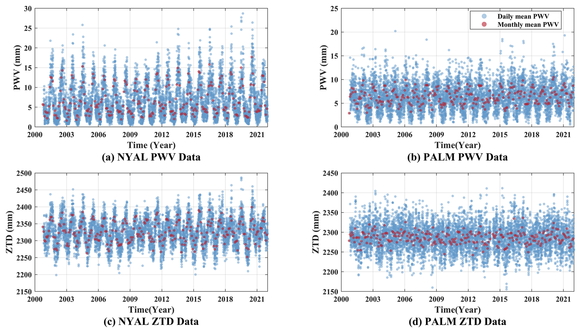
Figure 16 Time series of daily and monthly mean PWV and ZTD values at the NYAL and PALM sites over the study period.

Daily mean values exhibit more pronounced variations and a wider range of extreme values, as they are prone to impact from typical weather extremes and atmospheric conditions. In contrast, monthly mean values, as aggregates of daily data, tend to smooth out these extremes (noises) and reduce short-term fluctuations, leading to a more stable trend. From another perspective, the temporal resolution of daily means is reduced by a factor of 24 compared to hourly estimates, but it is still over 30 times higher than that of monthly averages. Therefore, with a larger volume of data, daily means are better suited for analysing short-term meteorological phenomena, while monthly means, by providing a clearer picture of month-to-season variations, more accurately capture general climate features and are more ideal for studying long-term trends, climate variability, and abnormal climate patterns. In general, hourly, daily, and monthly data each play an essential role in atmospheric studies. Understanding data characteristics across these time scales is crucial for effective utilisation of this information in various applications.

Following a similar approach as in Sect. 4, we also assessed the quality of the determined daily and monthly mean PWVs by using the ERA5 dataset as an external reference. Specifically, we evaluated the performance of daily and monthly mean values of PWV by comparing them against the ERA5 dataset across all the sites adopted in this study. Figure 17 presents the bias and RMS results over the period 2001–2021. Note that the bias values are calculated by subtracting the PWVs obtained from the ERA5 dataset from those derived from GPS observations.

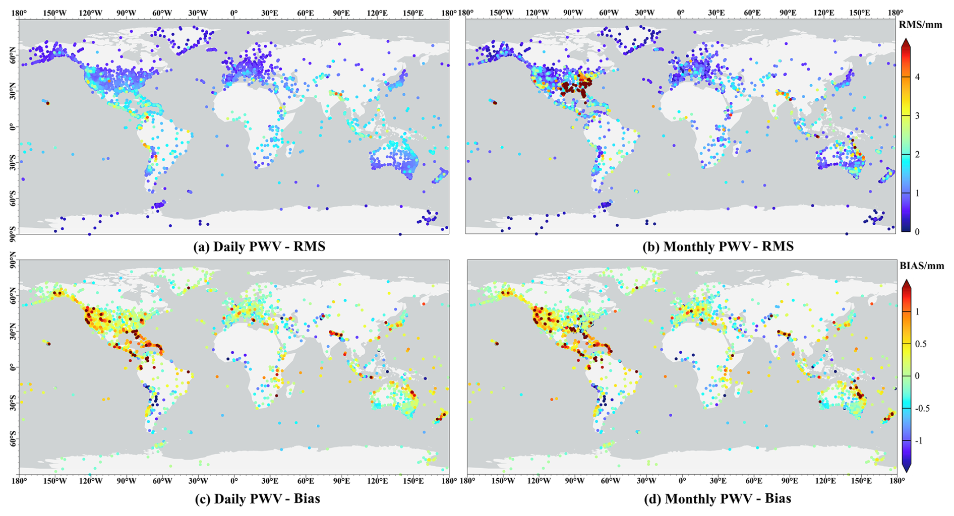
Figure 17 RMS (a, b) and Bias (c, d) statistics resulting from the comparison of daily and monthly mean PWV at all the stations against ERA5 dataset over the whole study period.

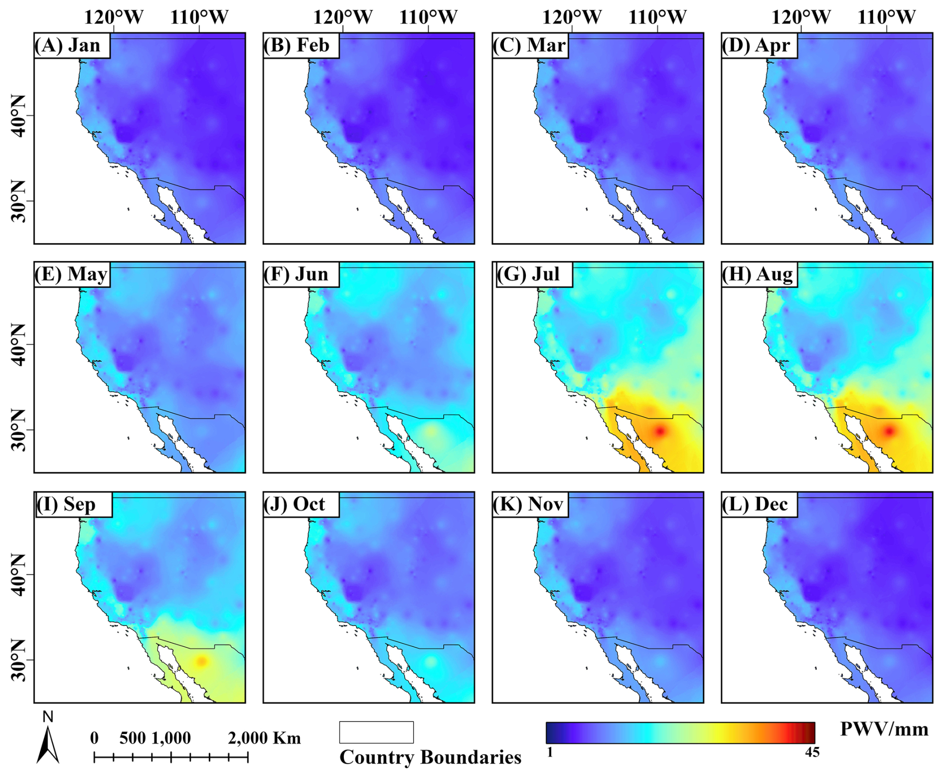
Figure 18 Rendered images of the 16-year climatological monthly mean PWV values for each month, derived from 590 GNSS sites located on the West Coast of the United States.

The RMS quantifies the overall agreement between the datasets by measuring the magnitude of error, independent of direction. As illustrated in Fig. 17a and b, the RMS exhibits a certain degree of latitude dependence, with higher values concentrated in low-latitude areas, specifically between 30° N and 30° S. This pattern can be attributed to the relatively larger PWV values and more pronounced variations in equatorial regions, as discussed in Sect. 5.1. Additionally, the sparse coverage of GNSS sites in these regions likely exacerbates this effect, as the limited number of data available constrains the robustness of data screening and quality control processes. In contrast, RMS values at sites in high-latitude regions are close to zero. Furthermore, a detailed comparison of Fig. 17a and b indicates that monthly RMS values are generally smaller than daily RMS values, suggesting closer alignment between monthly means of the two datasets. This is largely attributed to the smoothing effect, narrower data range, and reduced data volume associated with monthly means. Regarding bias analysis, which captures the systematic offset or average deviation between two datasets, a similar latitude-dependent pattern is observed. However, since bias indicates the direction of deviation, an additional finding is that most positive bias values are found at sites in low-latitude regions, indicating that PWVs derived from GPS data are generally higher than those from the ERA5, consistent with findings in Yu et al. (2021). Note that this pattern is not absolute, as some low-latitude stations also exhibit negative bias values, probably due to factors like local climate conditions, latitude, and data processing differences.

To add depth to the analysis, we examined the monthly characteristics of PWV values. Specifically, we calculated the average values of the monthly mean PWV for each month across all sites over the 16-year period 2006–2021, providing a climatological perspective across this span. The selection of the period is to mitigate the impact of missing data in the earlier years, i.e. 2001–2005 and ensures the quality of the determined 16-year climatological monthly mean PWVs. Figure 18 presents the rendered images of these average monthly mean PWVs for each month, derived from 590 GNSS stations located on the West Coast of the United States. This study region was chosen due to its relatively dense GNSS network, which enhances the accuracy and robustness of the 16-year climatological monthly mean PWV representations. Notwithstanding, this figure is mainly intended for regional-scale visualisation and qualitative analysis, given the uneven station spacing, they should not be interpreted at fine spatial scales.

It can be found that the highest PWV values typically occur in July and August, while lower PWVs are observed in December, January, and February. As the study region is in the northern hemisphere, these months correspond to the summer and winter seasons, respectively, highlighting clear seasonal variation features in PWV. Specifically, the higher PWV estimates observed in summer are largely due to elevated temperatures, which increase the moisture-holding capacity of the atmosphere. As per the empirical Clausius–Clapeyron equation, a 1 K increase in temperature can result in an approximate 7 % increase in PWV, indicating that warmer air in summer can retain more water vapour (O'Gorman and Muller, 2010). Additionally, during summer, higher temperatures and stronger solar radiation boost evaporation from surface water sources, while prevailing winds carry this moist air inland, further raising atmospheric water vapour levels. The combination of these factors directly contributes to the pronounced seasonal increase in PWV during summer months.

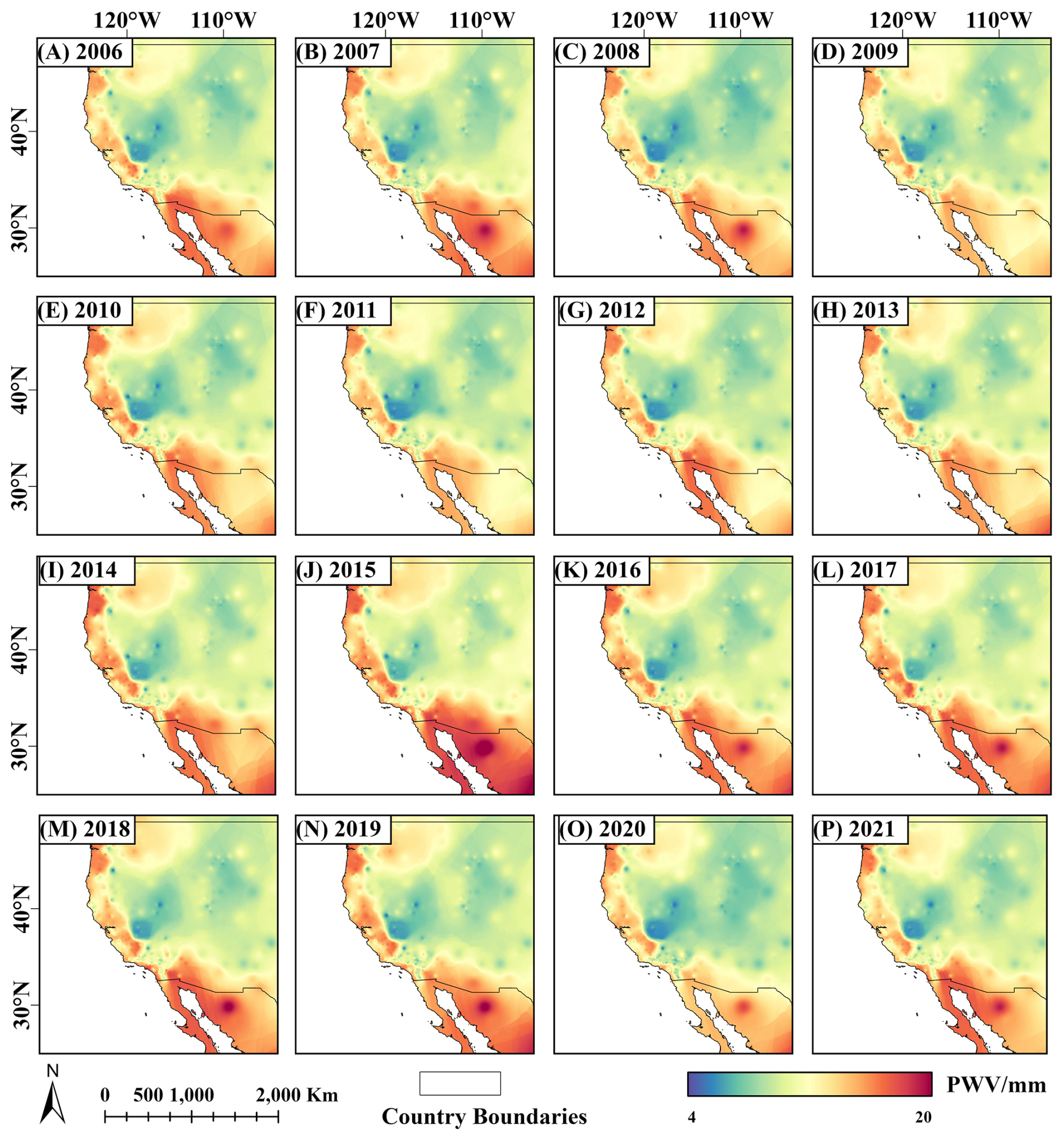
Figure 19 Rendered images of the annual mean PWV values for each year over the 16-year period 2006–2021, calculated from 590 GNSS sites located on the West Coast of the United States.

5.3 Analysis of annual mean PWV estimates

In addition to examining PWV estimates at hourly, daily and monthly scales, this study extends the analysis to annual mean PWV values, as annual averages of ECVs are commonly used in climate studies, especially for analysing long-term trends (Coldewey-Egbers et al., 2022; John and Soden, 2007; Masson-Delmotte et al., 2021; Sherwood et al., 2010). Following the established guidelines for calculating diurnal and monthly mean PWV, only GNSS stations with consistent PWV data over the period 2006–2021 were adopted to maintain the quality of the annual mean values. Figure 19 depicts rendered images of the annual mean PWV for each year over the 16-year period, calculated from 590 GNSS sites located on the West Coast of the United States. As with the monthly fields, the rendering is also qualitative at sub-regional scales. Users seeking local detail in future applications should restrict analyses to smaller areas with denser network coverage.

Three main phenomena can be observed from the statistical analysis of the calculated annual mean PWV, together with the visual examination of Fig. 19. First, an overall analysis reveals that the long-term trend of PWV shows a general increase over the whole 16-year period, aligning closely with the recorded temperature rise in the region (Masson-Delmotte et al., 2021). This phenomenon can be explained by the same principles linking temperature and water vapour discussed in Sect. 5.2.

Secondly, it was found that the highest annual PWV for an individual GNSS site was observed at the p501 site in 2015, with a value of 18.8 mm. Moreover, the highest mean PWV across all analysed stations also occurred in 2015, reaching 13.41 mm. This peak likely represents the co-occurrences of the strong 2015/2016 El Niño (L'Heureux et al., 2017) and the North Pacific marine heatwave known as “the Blob”, a significant mass of relatively warm water in the northeast Pacific Ocean off the coast of the United States (Bond et al., 2015; Di Lorenzo and Mantua, 2016; Peterson et al., 2015). Together, these phenomena generated positive temperature anomalies exceeding 2.5 °C, with the warm ocean surface heating the overlying atmosphere. For example, according to the statistics from the National Oceanic and Atmospheric Administration (NOAA), in 2015, the annual mean temperatures in States in the study region such as California, Oregon, and Washington were elevated compared to normal conditions, with values of 17.0, 12.2, and 11.1 °C, respectively. Moreover, the increase in sea surface temperature also led to higher evaporation rate, resulting in enhanced atmospheric moisture and increased water vapour.

Lastly, at the opposite end of the spectrum, the lowest annual PWV recorded for a single station was 4.5 mm at the LEWI station in 2008. Despite this, the lowest mean PWV across all stations was observed in 2020, with the value of 11.96 mm. As per Voosen (2021), based on average readings from thousands of in-situ weather stations and ocean probes, the planet in 2020 was approximately 1.25 °C warmer than in preindustrial times, matching record-high temperatures. While an increase in temperature typically corresponds to higher water vapour content, the anomalously low PWV can be attributed to climate extremes in this region. For example, unprecedented high temperatures were recorded across many parts of the region in 2020, leading to prolonged heatwaves and exceptionally low humidity. Typically, in the Santa Ynez Valley of southern California, several sites set all-time temperature records, with the highest reaching 48.3 °C (Duine et al., 2022). In August 2020, Death Valley, California, reported a temperature of 54.4 °C, the highest globally recorded since 1931 (Blunden and Boyer, 2021). Additionally, in September 2020, Oregon and California experienced a series of wildfires, burning 1.2 million acres and contributing to significant low-humidity conditions (Abatzoglou et al., 2021; Khorshidi et al., 2020). During these extremes, near-surface specific humidity levels in the western Oregon Cascades dropped to just 3.3 g m⁻³. From an atmospheric physics perspective, the smoke plumes from these wildfires increased aerosol optical depth, which, through complex interactions between aerosols, radiation, and the boundary layer, intensified local thermal circulations. This, in turn, also led to stronger winds and reduced humidity levels (Huang et al., 2023). Overall, while it is crucial to use a wide range of ECVs to effectively monitor climate change, these findings provide preliminary evidence that the annual mean estimates of GNSS atmospheric parameters can serve as a valuable and complementary tool for more comprehensive assessments of climate changes and associated climate risks.

6 Data availability

The global GNSS climate data record, including hourly ZTD and PWV estimates, described in this work is now available at: https://doi.org/10.1594/PANGAEA.982476 (Wang et al., 2025a). The datasets have also been made available through the GPAC data portal: https://www.gnss.studio/Login (Wang et al., 2025b), with its data download interface shown in Fig. 20.

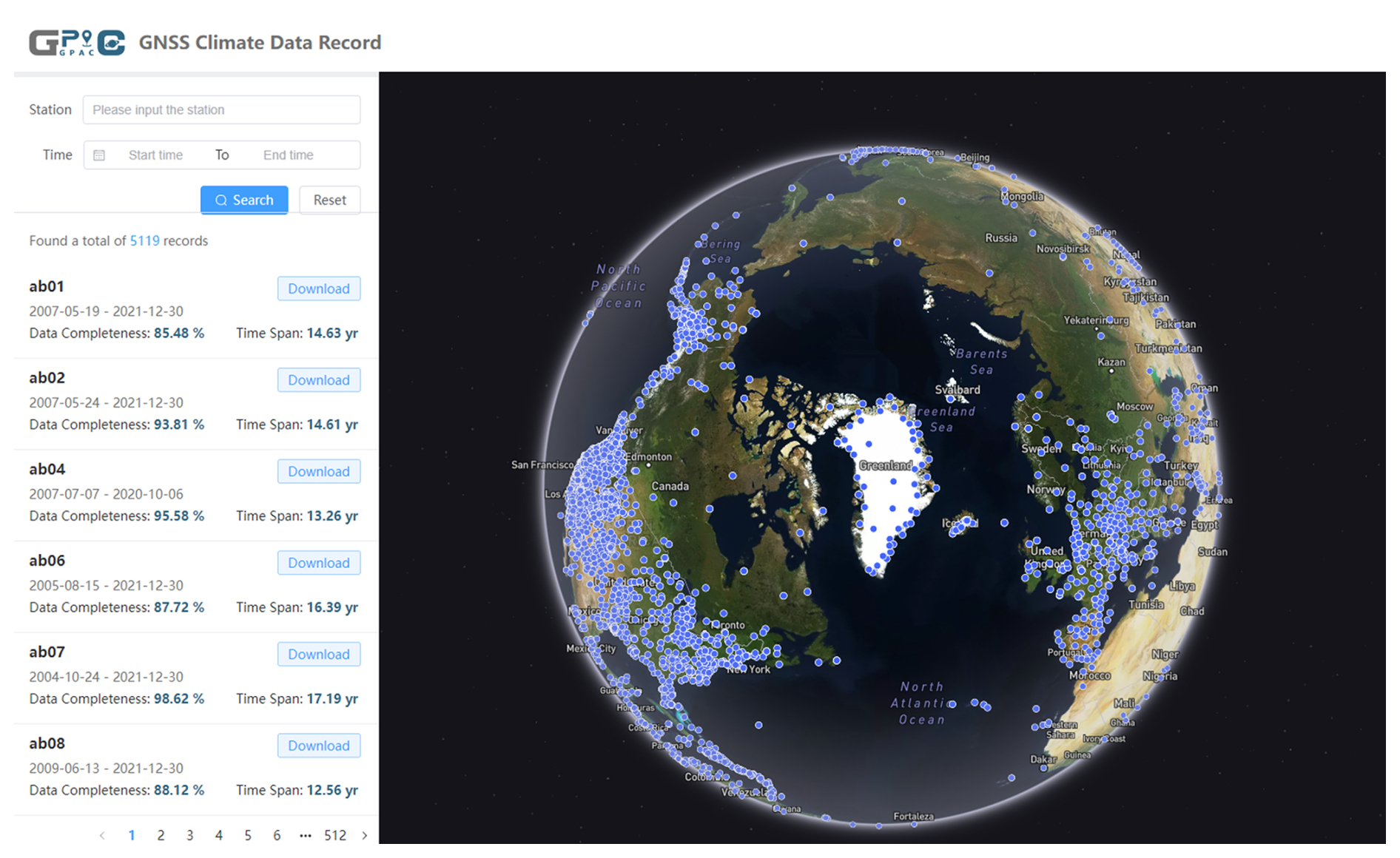
Figure 20 Download interface of the reprocessed GNSS climate data record.

7 Summary and outlook

This study has produced a global GNSS climate data record to help address data gaps in existing climate observing networks. Spanning up to a 22-year period from 2000 to 2021, the dataset includes hourly ZTD and PWV estimates from 5085 sites, providing broad spatiotemporal coverage and good overall accuracy globally. Advanced data reprocessing strategies, aligned with the IGS standards, were used to promote the consistency and accuracy of the generated atmospheric parameters, enhancing their suitability for climate applications. The quality of the dataset was evaluated via a rigorous quality assessment framework and cross-comparisons with various external references, including ERA5 reanalysis dataset, sounding profiles, and VLBI measurements. Generally good agreement across these datasets was demonstrated, with consistent water vapour estimates across diverse geographic and climate conditions. The dataset represents a critical step in GNSS climatology, offering valuable insights into the spatiotemporal variability of atmospheric water vapour. Further analyses of diurnal, monthly, seasonal, and annual variations in ZTD and PWV highlighted their importance in understanding climate variability, including responses to weather extremes and long-term climate trends.

Despite these advancements, several key challenges and opportunities for improvement remain. First, while this study mainly employed GPS observations, integrating multi-GNSS systems such as Galileo, GLONASS, and BeiDou could improve satellite visibility and geometry, and may enhance spatiotemporal availability and robustness, particularly in under-represented regions like polar areas and oceans. However, as noted in Sect. 2.2, introducing additional constellations can impose inter-system biases and calibration complexities that may induce shifts in the time series. In other words, the net benefit is context-dependent and not yet settled. Given this, our ongoing research is conducting a new reprocessing campaign that will incorporate multi-GNSS observations using the latest Bernese V5.4 and updated tropospheric models like VMF3, while managing inter-system and inter-frequency biases, harmonising antenna calibrations and metadata, and ensuring cross-system consistency. Second, although the generated dataset covers up to 22 years and can support climate applications, it does not yet meet the “30-year” timescale typically required for climatology, largely because most GNSS stations lack sufficiently long historical observations as stated earlier. Accordingly, we aim to continuously process new data streams to extend the record beyond 30 years and provide a more complete dataset. Thirdly, the refinement of data retrieval techniques is necessary to address challenges posed by complex topographies and high-altitude regions, thereby improving robustness in these environments. In particular, the ZHD estimation choice adopted in this study may influence PWV at some certain sites and times, in our next reprocessing, we will document and benchmark the differences between approaches. Additionally, the incorporation of GNSS atmospheric parameters into global reanalysis datasets and climate models is also expected to bridge existing gaps in Earth observation networks and significantly advance climate applications. Lastly, emerging digital innovation techniques, such as artificial intelligence and digital-twin techniques, are considered promising for extracting deeper insights from the dataset. Collaborative efforts with international stakeholders, such as the World Meteorological Organization (WMO), IGS, and International Association of Geodesy (IAG), are expected to further enable the impact of the dataset and ensure its alignment with global research priorities.

Overall, the generated dataset represents a meaningful step toward fully harnessing the transformative potential of GNSS atmospheric monitoring techniques for advancing climate and atmospheric studies. By addressing critical challenges and leveraging cutting-edge methods, this dataset provides a reference for GNSS climatology, offering a foundation for future research and operational applications across this interdisciplinary field. These contributions may enhance our understanding of atmospheric dynamics, supporting sustainable development and facilitating informed decision-making.