CEDAR-GPP: spatiotemporally upscaled estimates of gross primary productivity incorporating CO₂ fertilization

Gross primary productivity (GPP) is the largest carbon flux in the Earth system, playing a crucial role in removing atmospheric carbon dioxide and providing carbohydrates needed for ecosystem metabolism. Despite the importance of GPP, however, existing estimates present significant uncertainties and discrepancies. A key issue is the underrepresentation of the CO₂ fertilization effect, a major factor contributing to the increased terrestrial carbon sink over recent decades. This omission could potentially bias our understanding of ecosystem responses to climate change.

Here, we introduce CEDAR-GPP, the first global machine-learning-upscaled GPP product that incorporates the direct CO₂ fertilization effect on photosynthesis. Our product is comprised of monthly GPP estimates and their uncertainty at 0.05° resolution from 1982 to 2020, generated using a comprehensive set of eddy covariance measurements, multi-source satellite observations, climate variables, and machine learning models. Importantly, we used both theoretical and data-driven approaches to incorporate the direct CO₂ effects. Our machine learning models effectively predict monthly GPP (R² ∼ 0.72), the mean seasonal cycles (R² ∼ 0.77), and spatial variabilities (R² ∼ 0.63) based on cross-validation at flux sites. After incorporating the direct CO₂ effects, the predicted long-term GPP trend across global flux towers substantially increases from 3.1 to 4.5–5.4 gC m⁻² yr⁻¹, which aligns more closely with the 7.7 gC m⁻² yr⁻¹ trend detected from eddy covariance data. While the global patterns of annual mean GPP, seasonality, and interannual variability generally align with existing satellite-based products, CEDAR-GPP demonstrates higher long-term trends globally after incorporating CO₂ fertilization and reflected a strong temperature control on direct CO₂ effects. The estimated global GPP trend is 0.57–0.76 PgC yr⁻¹ from 2001 to 2018 and 0.32–0.34 PgC yr⁻¹ from 1982 to 2018. Estimating and validating GPP trends in data-scarce regions, such as the tropics, remains challenging, underscoring the importance of ongoing ground-based monitoring and advancements in modeling techniques. CEDAR-GPP offers a comprehensive representation of GPP temporal and spatial dynamics, providing valuable insights into ecosystem–climate interactions. The CEDAR-GPP product is available at https://doi.org/10.5281/zenodo.8212706 (Kang et al., 2024).

1 Introduction

Terrestrial ecosystem photosynthesis, known as Gross primary productivity (GPP), is the primary source of food and energy for the Earth system and human society (Keenan and Williams, 2018). Through photosynthesis, terrestrial ecosystems also mitigate climate change, by removing 30 % of anthropogenic carbon emissions from the atmosphere each year (Friedlingstein et al., 2023). However, due to the lack of direct measurements at the global scale, our understanding of photosynthesis and its spatiotemporal dynamics is limited, leading to considerable disagreements among various GPP estimates (Anav et al., 2015; O'Sullivan et al., 2020; Smith et al., 2016; Yang et al., 2022). Addressing these uncertainties is crucial for improving the predictability of ecosystem dynamics under climate change (Friedlingstein et al., 2014).

Over the past three decades, global networks of eddy covariance flux towers collected in situ carbon flux measurements that allow for accurate estimates of GPP, providing valuable insights into photosynthesis dynamics under various environmental conditions (Baldocchi, 2020; Beer et al., 2010). To quantify and understand GPP at scales and locations beyond the ∼ 1 km² flux tower footprints, machine learning has been employed with gridded satellite and climate datasets to upscale site-based measurements and produce wall-to-wall GPP maps (Dannenberg et al., 2023; Joiner and Yoshida, 2020; Jung et al., 2011; Tramontana et al., 2016; Xiao et al., 2008; Yang et al., 2007; Zeng et al., 2020). This “upscaling” approach provides data-driven and observation-based quantifications without prescribed functional relations between GPP and its climatic or environmental drivers. It offers unique empirical constraints of ecosystem carbon dynamics, complementing those derived from process-based and semi-process-based approaches such as terrestrial biosphere models or the light-use efficiency (LUE) models (Beer et al., 2010; Gampe et al., 2021; Jung et al., 2017; Schwalm et al., 2017). In recent years, the growth of global and regional flux networks, coupled with increasing efforts in data standardization, has offered new opportunities for the advancement of upscaling frameworks, enabling comprehensive quantifications of terrestrial photosynthesis (Joiner and Yoshida, 2020; Nelson et al., 2024; Pastorello et al., 2020).

Effective machine learning upscaling depends on a complete set of input predictors that fully explain GPP dynamics. Upscaled datasets have primarily relied on satellite-observed greenness indicators, such as vegetation indices, leaf area index (LAI), and the fraction of absorbed photosynthetically active radiation (fAPAR), which effectively capture canopy-level GPP dynamics related to leaf area changes (Joiner and Yoshida, 2020; Ryu et al., 2019; Tramontana et al., 2016). However, important aspects of leaf-level physiology, such as those controlled by climate factors, are often omitted in major upscaled datasets, preventing accurate characterization of GPP responses to climate change (Bloomfield et al., 2023; Stocker et al., 2019). In particular, none of the previous upscaled datasets have considered the direct effect of atmospheric CO₂ on leaf-level photosynthesis, which is a key factor contributing to at least half of the enhanced land carbon sink observed over the past decades (Keenan et al., 2016, 2023; Ruehr et al., 2023; Walker et al., 2021). This omission can lead to incorrect inferences regarding long-term trends in various components of the terrestrial carbon cycle (De Kauwe et al., 2016).

Multiple independent lines of evidence from atmospheric inversion (Wenzel et al., 2016), atmospheric ¹³C $/$ ¹²C measurements (Keeling et al., 2017), ice core records of carbonyl sulfide (Campbell et al., 2017), glucose isotopomers (Ehlers et al., 2015), as well as free-air CO₂ enrichment experiments (FACE) (Walker et al., 2021), suggest a widespread positive effect of elevated atmospheric CO₂ on GPP from site to global scales. Increasing atmospheric CO₂ directly stimulates the biochemical rate or the LUE of leaf-level photosynthesis, known as the direct CO₂ fertilization effect (CFE). Enhanced photosynthesis could lead to greater net carbon assimilation, contributing to an increase in total leaf area. This expansion, contributing to higher light interception, further enhances canopy-level photosynthesis (i.e., GPP), which is referred to as the indirect CFE. The direct CFE has been found to dominate GPP responses to CO₂ compared to the indirect effect, from both theoretical and observational analyses (Chen et al., 2022; Haverd et al., 2020; Keenan et al., 2023).

Satellite-based estimates have shown an increasing global GPP trend in the past few decades, largely attributable to CO₂-induced increases in LAI (Chen et al., 2019; De Kauwe et al., 2016; Piao et al., 2020; Zhu et al., 2016). However, previous upscaled GPP datasets, as well as most LUE models such as the MODIS GPP product, have failed to consider the direct CO₂ effects on leaf-level biochemical processes (Jung et al., 2020; Zheng et al., 2020). Consequently, these products likely underestimated the long-term trend of global GPP, leading to large discrepancies when compared to process-based models, which typically consider both direct and indirect CO₂ effects (Anav et al., 2015; De Kauwe et al., 2016; Keenan et al., 2023; O'Sullivan et al., 2020). Notably, recent improvements in LUE models have included the CO₂ response and show improved long-term changes in GPP globally (Zheng et al., 2020), yet this important mechanism is still missing in GPP products upscaled from in situ eddy covariance flux measurements based on machine learning models.

To improve the quantification of GPP spatial and temporal dynamics and provide a robust representation of long-term dynamics in global photosynthesis, we developed the CEDAR-GPP¹ data product. CEDAR-GPP was upscaled from global eddy covariance carbon flux measurements using machine learning along with a broad range of multi-source satellite observations and climate variables. In addition to incorporating direct CO₂ fertilization effects on photosynthesis, we also account for indirect effects via greenness indicators and include novel satellite datasets such as solar-induced fluorescence (SIF), land surface temperature (LST), and soil moisture to explain variability under environmental stresses. We provide monthly GPP estimations and associated uncertainties at 0.05° resolution derived from 10 model setups. These setups differ by the temporal range depending on satellite data availability, the method for incorporating the direct CO₂ fertilization effects, and the partitioning approach used to derive GPP from eddy covariance measurements. Short-term model setups are primarily based on data derived from MODIS satellites generating GPP estimates from 2001 to 2020, while long-term estimates span 1982 to 2020 using combined Advanced Very-High-Resolution Radiometer (AVHRR) and MODIS data. We used two approaches to incorporate the direct CO₂ fertilization effects, including direct prescription with eco-evolutionary theory and machine learning inference from the eddy-covariance data. Additionally, we provide a baseline configuration that does not incorporate the direct CO₂ effects. Uncertainties in GPP estimation were quantified using bootstrapped model ensembles. We evaluated the machine learning models' skills in predicting monthly GPP, seasonality, interannual variability, and trend against eddy covariance measurements, and compared the CEDAR-GPP spatial and temporal variability to existing satellite-based GPP estimates.

2 Data and methods

2.1 Eddy covariance data

We obtained monthly eddy covariance GPP measurements from 2001 to 2020 from the FLUXNET2015 (Pastorello et al., 2020), AmeriFlux FLUXNET (https://ameriflux.lbl.gov/data/flux-data-products/, last access: 2 January 2022), and ICOS Warm Winter 2020 (Warm Winter 2020 Team, 2022) datasets. All data were processed with the ONEFLUX pipeline (Pastorello et al., 2020). Following previous upscaling efforts (Tramontana et al., 2016), we selected monthly GPP data with at least 80 % of high-quality hourly or half-hourly data for temporal aggregation. High-quality data refers to GPP derived from measured or high-quality gap-filled net ecosystem exchange (NEE) data. We further excluded large negative GPP values, setting a cutoff of −1 gC m⁻² d⁻¹. We utilized GPP estimates from both the night-time (GPP_REF_NT_VUT) and day-time (GPP_REF_ DT_VUT) partitioning approaches. We classified flux tower sites according to the C₃ and C₄ plant categories reported in metadata and related publications when available and used a C₄ plant percentage map (Still et al., 2003) otherwise. This classification information is included in Sect. S1 in the Supplement. Our analysis encompassed 233 sites, predominantly located in North America, Western Europe, and Australia (Fig. 1). A list of the sites is provided in Appendix A. Despite their uneven geographical distribution, these sites effectively cover a diverse range of climatic conditions and are representative of global biomes (Fig. 1c, d). In total, our dataset included over 18 000 site-months. Note that we did not include eddy covariance data before 2001 since it was limited to only a few sites, with only four sites containing data before 1996. This scarcity might introduce biases in the machine learning models, particularly in the relationship between GPP and CO₂, leading to unreliable extrapolations across space and time in the long-term predictions.

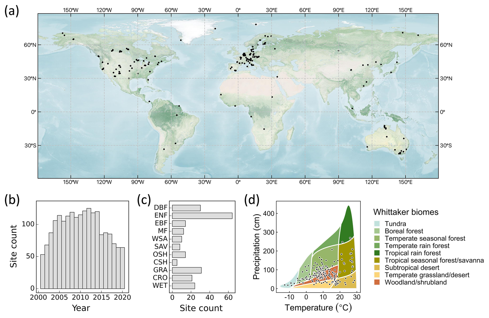
Figure 1 (a) Spatial distribution of eddy covariance sites used to generate the CEDAR-GPP product. (b) Annual site counts. (c) Site counts by biomes. ENF: evergreen needleleaf forests; EBF: evergreen broadleaf forests; DBF: deciduous broadleaf forest; MF: mixed forests; WSA: woody savannas; SAV: savannas; OSH: open shrublands; CSH: closed shrublands; GRA: grasslands; CRO: croplands; WET: wetlands. (d) Site distributions in the annual temperature and precipitation space. Whittaker biome classification is shown as a reference of natural vegetation based on long-term climatic conditions. It does not directly indicate the actual biome associated with each site. The base map in (a) was obtained from the NASA Earth Observatory map by Joshua Stevens using data from NASA's MODIS Land Cover, the Shuttle Radar Topography Mission (SRTM), the General Bathymetric Chart of the Oceans (GEBCO), and Natural Earth boundaries. Whittaker biomes were plotted using the “plotbiomes” R package (Ştefan and Levin, 2018).

2.2 Global input datasets

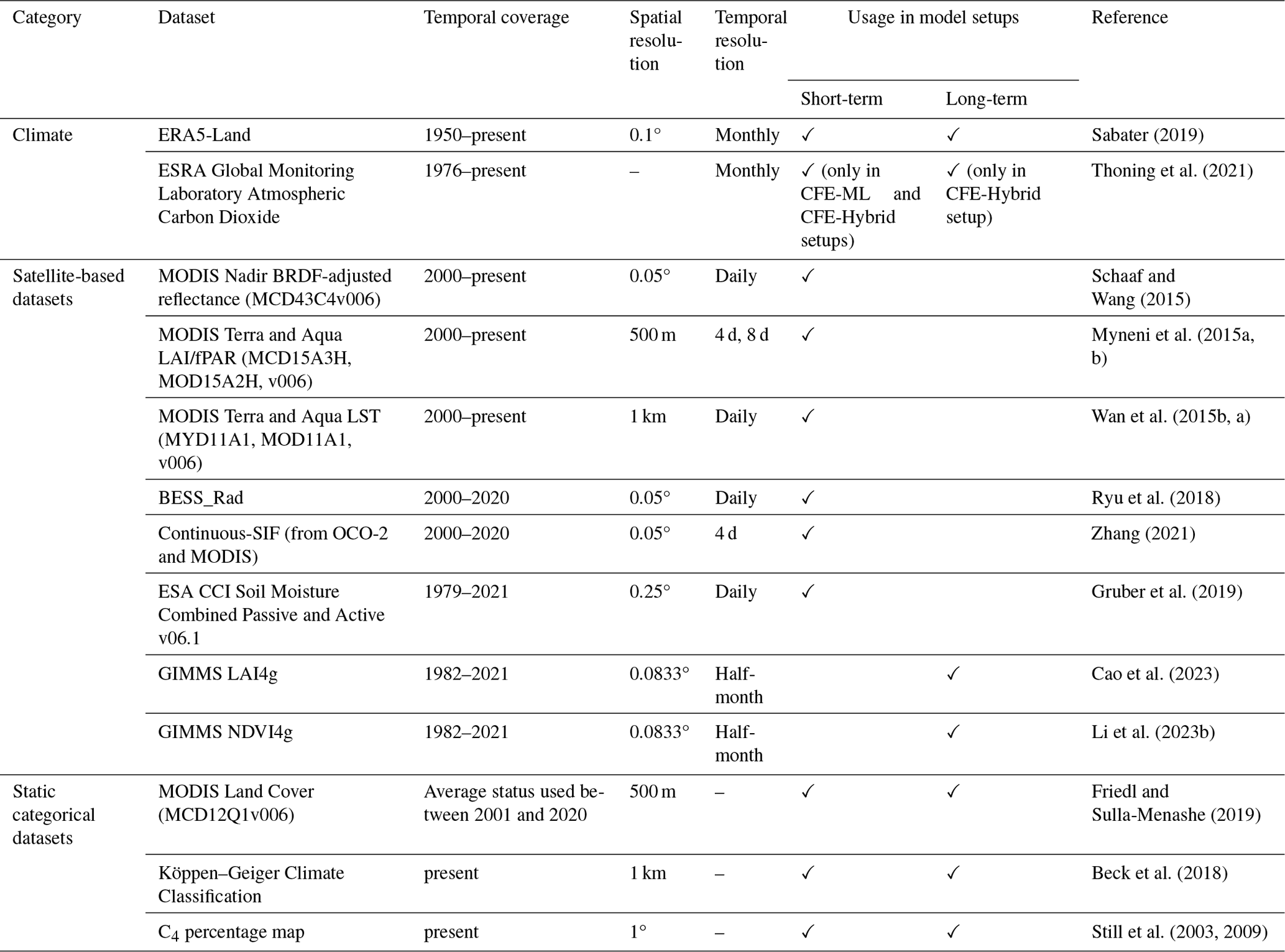
We compiled an extensive set of covariates from gridded climate reanalysis data; multi-source satellite datasets including optical, thermal, and microwave observations; and categorical information on land cover, climate zone, and C₃ $/$ C₄ classification. The datasets that we compiled offer comprehensive information about GPP dynamics and its responses to climatic variabilities and stresses. Table 1 lists the datasets and associated variables used to generate CEDAR-GPP.

Table 1 Datasets used in different model setups to generate the CEDAR GPP product. Refer to Table S1 in the Supplement for a list of specific variables from each dataset.

2.2.1 Climate variables

We obtained air temperature, vapor pressure deficit, precipitation, potential evapotranspiration, and skin temperature from the EAR5-Land reanalysis dataset (Sabater, 2019; Tables 1, S1). We applied a three-month lag to precipitation, to represent the root zone water availability. Averaged monthly atmospheric CO₂ concentrations were calculated as an average of records from the Mauna Loa Observatory and South Pole Observation stations, retrieved from NOAA's Earth System Research Laboratory (Thoning et al., 2021).

2.2.2 Satellite datasets

We assembled a broad collection of satellite-based observations of vegetation greenness and structure, LST, solar radiation, solar-induced fluorescence (SIF), and soil moisture (Tables 1, S1).

We used three MODIS version 6 products: surface reflectance, LAI/fAPAR, and LST. Surface reflectance from optical to infrared bands (band 1 to 7) was sourced from the MODIS Nadir BRDF-adjusted reflectance (NBAR) daily dataset (MCD43C₄; Schaaf and Wang, 2015). From these data, we derived vegetation indices, including NIRv (Badgley et al., 2019), kNDVI (Camps-Valls et al., 2021), NDVI, enhanced vegetation index (EVI), normalized difference water index (NDWI) (Gao, 1996), and the green chlorophyll index (CIgreen; Gitelson, 2003). We also used snow percentages from the NBAR dataset. We used the 4 d LAI and fPAR composite derived from Terra and Aqua satellites (MCD15A3H; Myneni et al., 2015a; Yan et al., 2016a, b) from July 2002 onwards and the MODIS 8 d LAI and fPAR dataset from Terra only (MOD15A2H) prior to July 2002 (Myneni et al., 2015b). We used day-time and night-time LST from the Aqua satellite (MYD11A1; Wan et al., 2015b), with the Terra-based LST product (MOD11A1) used after July 2002 (Wan et al., 2015a). Terra LST was bias-corrected with the differences in the mean seasonal cycles between Aqua and Terra following Walther et al. (2022).

We used the PKU GIMMS NDVI4g dataset (Li et al., 2023b) and PKU GIMMS LAI4g (Cao et al., 2023) datasets available from 1982 to 2020. PKU GIMMS NDVI4g is a harmonized time series that includes AVHRR-based NDVI from 1982 to 2003 (with biases and corrections mitigated through inter-calibration with Landsat surface reflectance images) and MODIS NDVI from 2004 onward. PKU GIMMS LAI4g consisted of consolidated AVHRR-based LAI from 1982 to 2003 (generated using machine learning models trained with Landsat-based LAI data and NDVI4g) and reprocessed MODIS LAI (Yuan et al., 2011) from 2004 onwards.

We utilized photosynthetically active radiation (PAR), diffusive PAR, and shortwave downwelling radiation from the BESS_Rad dataset (Ryu et al., 2018). We obtained the continuous-SIF (CSIF) dataset (Zhang, 2021; Zhang et al., 2018) produced by a machine learning algorithm trained using OCO-2 SIF observations and MODIS surface reflectance. We used surface soil moisture from the ESA CCI soil moisture combined passive and active product (version 6.1) (Dorigo et al., 2017; Gruber et al., 2019).

2.2.3 Other categorical datasets

We used plant functional type (PFT) information derived from the MODIS Land Cover product (MCD12Q1; Friedl and Sulla-Menashe, 2019). We followed the International Geosphere-Biosphere Program classification scheme but merged several similar categories to maximize the number of eddy covariance sites/observations available for each category. Closed and open shrublands are combined into a shrubland category. Woody savannas and savannas are combined into savannas. We generated a static PFT map by taking the mode of the MODIS land cover time series between 2001 and 2020 at each pixel to mitigate uncertainties from misclassification in the MODIS dataset. Nevertheless, changes in vegetation structure induced by land use and land cover change are reflected in the dynamic surface reflectance and LAI/fAPAR datasets we used. We used the Köppen–Geiger main climate groups (tropical, arid, temperate, cold, and polar; Beck et al., 2018). We also utilized a C₄ plant percentage map to account for different photosynthetic pathways when incorporating CO₂ fertilization (Still et al., 2003, 2009). The C₄ percentage dataset was constant over time.

2.2.4 Data preprocessing

We implemented a three-step preprocessing strategy for the satellite datasets: (1) quality control, (2) gap-filling, and (3) spatial and temporal aggregation. First, we selected high-quality data based on the quality control flags of the satellite products when available. For the MODIS NBAR dataset (MCD43C3), we used data with 75 % or more high-resolution NBAR pixels retrieved with full inversions for each band. For MODIS LST, we selected the best-quality data from the quality control bitmask as well as data where retrieved values had an average emissivity error of no more than 0.02. For MODIS LAI/fAPAR, we used retrievals from the main algorithm with or without saturation. We used all available data in ESA-CCI soil moisture due to the presence of substantial data gaps. In the gap-filling step, missing values in satellite datasets were temporally filled at the native temporal resolution, following a two-step protocol adapted from Walther et al. (2022). Short temporal gaps were first filled with medians from a moving window, and the remaining gaps were filled with the mean seasonal cycle. For datasets with a high temporal resolution, including MODIS NBAR (daily), LAI/fPAR (4 d), BESS (4 d), CSIF (4 d), and ESA-CCI (daily), temporal gaps no longer than 5 d (8 d for 4 d resolution products) were filled with medians of 15 d moving windows in the first step. An exception is MODIS LST (daily), for which we used a shorter moving window of 9 d due to rapid changes in surface temperature. GIMMS LAI4g and NDVI4g data were only filled with the mean seasonal cycle due to their low temporal resolution (half-month). This is because vegetation structure could experience significant changes at half-month intervals, and gap-filling using temporal medians within moving windows could introduce considerable uncertainties and potentially over-smooth the time series.

Finally, all the datasets were aggregated to a monthly time step and 0.05° spatial resolution. We employed the conservative resampling approach using the xESMF Python package (Zhuang et al., 2023). To generate the machine learning model training data, we extracted values from the nearest 0.05° pixel relative to the site locations within the gridded dataset.

Figure 2 Schematic overview of the CEDAR-GPP model setups.

2.3 Machine learning upscaling

2.3.1 CEDAR-GPP model setups

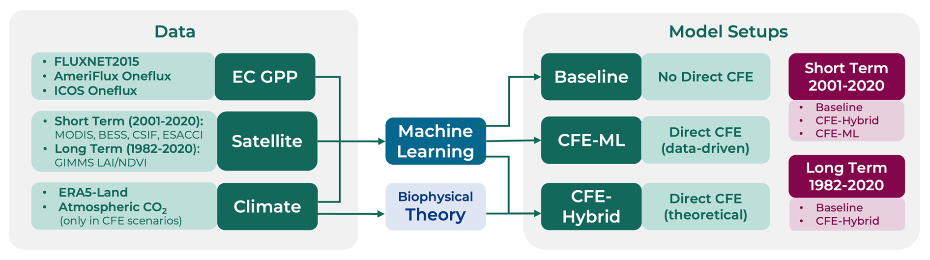
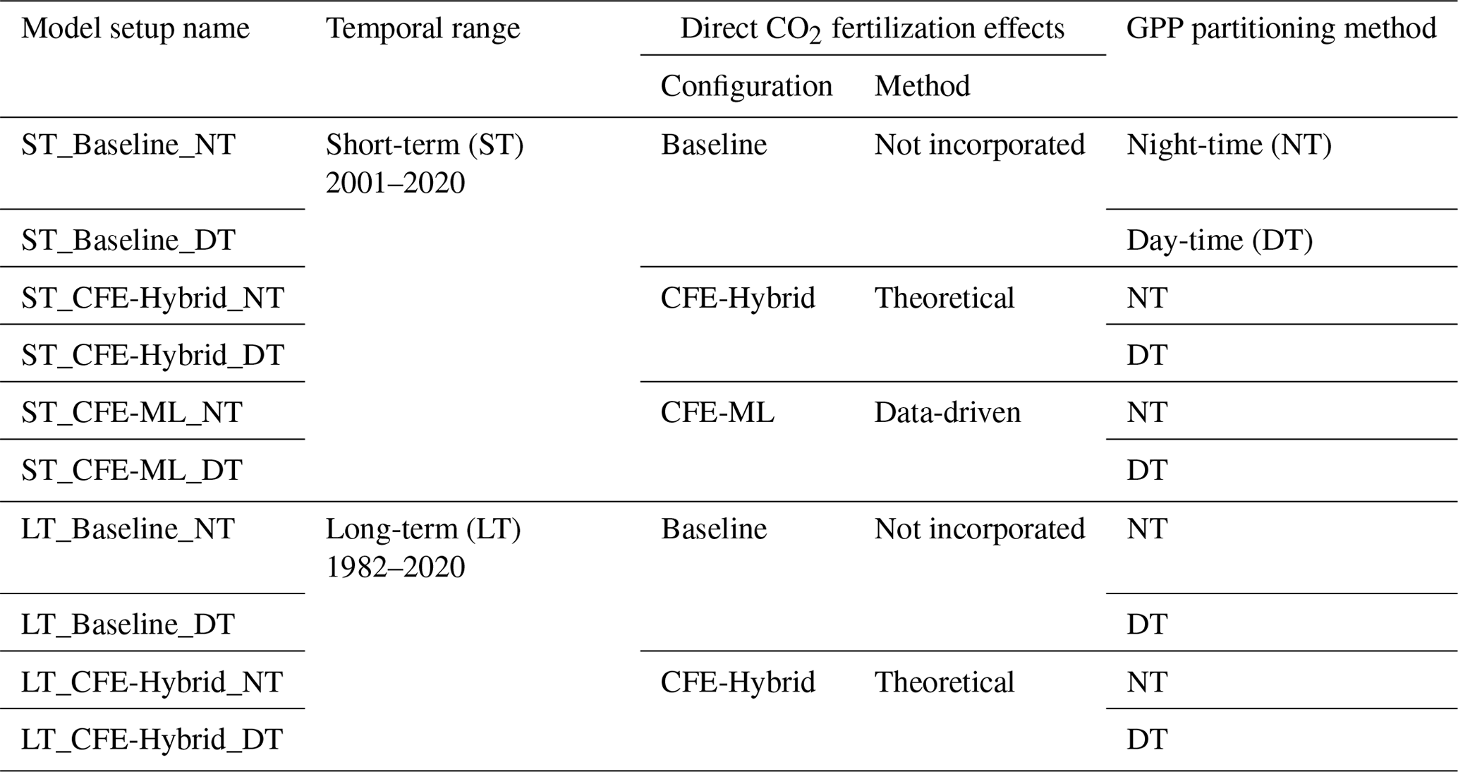
We trained machine learning models with eddy covariance GPP measurements as targets and climate/satellite variables as input features. We created 10 model setups to produce different global monthly GPP estimates (Fig. 2; Table 2). The model setups were characterized by the temporal range depending on input data availability, the configuration of CO₂ fertilization effects, and the partitioning approach used to derive the GPP from eddy covariance measurements.

The short-term (ST) model configuration produced GPP from 2001 to 2020, and the long-term (LT) configuration spanned 1982 to 2020. Each temporal configuration uses a different set of input variables depending on their availability. Inputs for the short-term configuration included MODIS, CSIF, BESS PAR, ESA-CCI soil moisture, ERA5-Land, as well as PFT and Köppen climate zone as categorical variables with one-hot encoding. The long-term configuration used GIMMS NDVI4g and LAI4g data, ERA5-land, PFT and Köppen climate. ESA CCI soil moisture datasets were excluded from the long-term model setups due to concerns about the product quality in the early years when the number and quality of microwave satellite data were limited (Dorigo et al., 2015). A detailed list of input features for each setup is provided in Table S1.

Regarding the direct CFE, we established a “Baseline” configuration that did not incorporate these effects, a “CFE-Hybrid” configuration that incorporated the effects via eco-evolutionary theory, and a “CFE-ML” configuration that inferred the direct effects from eddy covariance data using machine learning. Detailed information about these approaches is provided in Sect. 2.3.2. Furthermore, separate models were trained for GPP target variables from the night-time (NT) and day-time (DT) partitioning approaches.

Table 2 lists the characteristics of the 10 model setups. Due to the limited availability of eddy covariance observations before 2001, we did not apply the CFE-ML approach to the long-term setups. The CFE-ML model, when trained on data from 2001 to 2020 with atmospheric CO₂ ranging from 370 to 412 ppm, would not accurately predict GPP response to CO₂ for the period 1982–2000 when the CO₂ levels were markedly lower (340–369 ppm). This is because machine learning models, especially tree-based models, could not extrapolate beyond the range of the training data.

Table 2 Specifications of the CEDAR-GPP model setups.

2.3.2 CO₂ fertilization effect

We established three configurations regarding the direct CO₂ fertilization effects on photosynthesis. In the baseline configuration, we trained machine learning models with eddy covariance GPP, input climate, and satellite features, but excluding CO₂ concentration. As such, the models only include indirect CO₂ effects from the satellite-based proxies of vegetation greenness or structure representing changes in canopy light interception, and they do not consider the direct effect of CO₂ on leaf-level photosynthetic rates (or LUE). Our baseline model is therefore directly comparable to other satellite-derived GPP products that only account for indirect CO₂ effects (Joiner and Yoshida, 2020; Jung et al., 2020).

In the CFE-ML configuration, we added monthly CO₂ concentration into the feature set in addition to those incorporated in the baseline models. Models inferred the functional relationship between GPP and CO₂ from the eddy covariance data. They thus encompass both CO₂ fertilization pathways – direct effects on LUE and indirect effects from the satellite-based proxies of vegetation greenness and structure.

In the CFE-Hybrid configuration, we applied biophysical theory to estimate the response of LUE to elevated CO₂, i.e., the direct CFE (Appendix B). First, we estimated a reference GPP, where LUE was not affected by any increase in atmospheric CO₂, by applying the CFE-ML model with a constant atmospheric CO₂ concentration equal to the 2001 level while keeping all other variables temporally dynamic. Then, the impacts of CO₂ on LUE were prescribed onto the reference GPP estimates using a theoretical CO₂ sensitivity function of LUE according to the optimal coordination theory (Appendix B). The theoretical CO₂ sensitivity function represents a CO₂ sensitivity that is equivalent to that of the electron-transport-limited (light-limited) photosynthetic rate. When light is limited, elevated CO₂ suppresses photorespiration leading to increased photosynthesis at a lower rate than when photosynthesis is limited by CO₂ (Lloyd and Farquhar, 1996; Smith and Keenan, 2020). Thus, the CFE-Hybrid scenario provides a conservative estimation of the direct CO₂ effects on LUE. Note that the theoretical sensitivity function describes the fractional change in LUE due to direct CO₂ effects relative to a reference period (i.e., 2001). Therefore, we used the CFE-ML model to establish this reference GPP by fixing the CO₂ effects to the 2001 level, rather than simply using the GPP from the Baseline model in which the direct CO₂ effects were not represented. Long-term trends from the reference and the Baseline models are consistent.

For both CFE-ML and CFE-Hybrid scenarios, we made another conservative assumption that C₄ plants do not benefit from elevated CO₂, despite potential increases in photosynthesis during water-limited conditions due to enhanced water use efficiency (Walker et al., 2021). Data from flux tower sites dominated by C₄ plants were removed from our training set, so the machine learning models inferred CO₂ fertilization only from flux tower sites dominated by C₃ plants. When applying models globally, we assumed the reference GPP values (with constant atmospheric CO₂ concentration equal to the 2001 level) to represent C₄ plants, and GPP estimates from CFE-ML or CFE-Hybrid models were applied in proportion to the percentage of C₃ plants in a grid cell.

2.3.3 Machine learning model training and validation

We employed the state-of-the-art XGBoost machine learning model, known for its high accuracy in regression problems across various domains, including environmental and ecological predictions (Berdugo et al., 2022; Chen and Guestrin, 2016; Kang et al., 2020). XGBoost is a scalable and parallelized implementation of the gradient boosting technique that iteratively trains an ensemble of decision trees, with each iteration targeted at minimizing the residuals from the last iteration. A notable merit of XGBoost is its ability to make predictions in the presence of missing values, a common issue in remote sensing datasets. The model is also robust to multi-collinearity between the predictors in our dataset, particularly for the variables derived from MODIS data.

We used five-fold cross-validation for model evaluation. Training data was randomly split into five groups (folds), with each fold held out for testing while the remaining four folds were used for model training. We imposed two restrictions on fold splitting: each flux site was entirely assigned to a fold to test model performance over unseen locations; the random sampling was stratified based on PFT to ensure coverage of the full range of PFTs in both training and testing. Additionally, co-located sites, defined as those within 0.05° of each other, were also assigned to the same fold, as they were often set up as a cluster with different treatments. This approach avoids conflated estimates of model uncertainty, as these sites are not independent. We also used a nested-cross-validation strategy, during which we performed a randomized search of hyperparameters using three-fold cross-validation within the training set. The nested cross-validation was aimed at reducing the risk of overfitting and improving the robustness of the evaluation.

We assessed the models' ability to capture the temporal and spatial characteristics of GPP, including monthly GPP, mean seasonal cycles, monthly anomalies, and cross-site variability. Model performance was assessed separately for each model setup (Table 2) and summarized by PFT and Köppen climate zone. Mean seasonal cycles were calculated as the mean monthly GPP over the site observation period, and monthly anomalies were the residuals of monthly GPP after subtracting mean seasonal cycles. Monthly GPP averaged over years for each site was used to assess cross-site variability. Goodness-of-fit metrics include RMSE, bias, and coefficient of determination (R²).

To evaluate the models' ability to capture long-term GPP trends, we aggregated the monthly GPP to annual values following Chen et al. (2022), which detected the CO₂ fertilization effect across global eddy covariance sites. For sites with at least five years of observations, GPP anomalies were computed by subtracting the multi-year mean GPP from the annual GPP for each site. Anomalies were aggregated across sites to achieve a single multi-site GPP anomaly per year. We excluded a site-year if less than 11 months of data was available and used linear interpolation to fill the remaining temporal gaps. This resulted in 81 sites used in the GPP trend evaluation. We used the Sen slope and Mann–Kendall test to examine the GPP trends from 2002 to 2019, excluding 2001 and 2020, due to the limited number of available sites with more than five years of data. We further assessed the aggregated annual trend by grouping the sites based on plant functional types and the Köppen climate zones. Categories with less than six long-term sites available were excluded from the analysis, which includes EBF and Tropics.

To further analyze GPP responses to CO₂ in the CFE-ML models, we leveraged two explainable machine learning approaches: ALE (accumulated local effects; Apley and Zhu, 2020; Baniecki et al., 2021) and SHAP (Shapley additive explanations; Lundberg and Lee, 2017). SHAP is a model interpretation method derived from game theory, providing a value for each feature's contribution to a prediction, elucidating how each feature impacts the model's output in a specific instance. Conversely, ALE quantifies the average effect of a feature across the data, isolating its impact by aggregating local effects and avoiding the biases associated with correlated features.

2.3.4 Product generation and uncertainty quantification

In the CEDAR-GPP product we generated GPP estimates from 10 model setups by applying the model to global gridded datasets (Table 2). GPP estimates were named after the corresponding model setups. We used bootstrapping to estimate prediction uncertainties. For each model setup we generated 30 bootstrapped sample sets of eddy covariance data, which were then used to train an ensemble of 30 XGBoost models. The bootstrapping was performed at the site level, and each bootstrapped sample set contained around 140 to 150 unique sites, 17 000 to 19 000 site-months covering all PFTs. The relative PFT composition in the bootstrapped sample sites was consistent with the full dataset. Hyperparameters of the XGBoost models used in the final product generation are described in Sect. S2 in the Supplement. The 30 models trained with bootstrapped samples generated an ensemble of 30 GPP values. We provided the ensemble GPP mean and used standard deviation to indicate uncertainties, for each of the 10 model setups.

2.3.5 Product inter-comparison

We compared the global spatial and temporal patterns of CEDAR-GPP with other major satellite-based GPP products, including three machine learning upscaled and two LUE-based datasets. We obtained two FLUXCOM products (Jung et al., 2020), the latest version of FLUXCOM-RS (FLUXCOM-RSv006) available from 2001 to 2020 based on remote sensing (MODIS collection 6) datasets only, as well as the FLUXCOM-RS+METEO ensemble available between 1979 to 2018 and based on the climatology of remote sensing observations and ERA5 forcings (hereafter FLUXCOM-ERA5). We used FluxSat (Joiner and Yoshida, 2020), available from 2001 to 2019, which is an upscaled dataset based on MODIS NBAR surface reflectance and PAR from Modern-Era Retrospective analysis for Research and Applications 2 (MERRA-2). Importantly, FluxSat does not incorporate climate forcings. We used the MODIS GPP product (MOD17), available since 2001, which was generated based on MODIS fAPAR and LUE as a function of air temperature and vapor pressure deficit but not atmospheric CO₂ concentration (Running et al., 2015). We also used the rEC-LUE products, available from 1982 to 2018 and based on a revised LUE model that incorporated the effect of atmospheric CO₂ concentration and the fraction of diffuse PAR on LUE (Zheng et al., 2020). Additionally, to evaluate GPP trends we further included three process-based models forced by remote sensing data – BEPS (Leng et al., 2024), BESSv2 (Li et al., 2023a), and PML V2 (Zhang et al., 2019). These products estimate GPP by scaling leaf-level biochemical photosynthesis models to the canopy level, using satellite-derived vegetation structural variables such as LAI. All three products incorporate the direct CO₂ effects within their biochemical photosynthesis models.

All datasets were resampled to 0.1° spatial resolution, and a common mask for the vegetated land area was applied. We evaluated global mean annual GPP, mean seasonal cycle, interannual variability, and trend among different datasets, comparing them over a common time period determined by their data availability. Global total GPP was computed by scaling the global area-weighted average GPP flux with the global land area (122.4 million km²) following Jung et al. (2020). Mean seasonal cycle was defined as in Sect. 2.3.3. We used the standard deviation of annual GPP to indicate the magnitude of interannual variability, the Sen slope to indicate the GPP annual trend, and the Mann–Kendall test for the statistical significance of trends.

3 Results

3.1 Evaluation of model performance

3.1.1 Overall performance

The short-term and long-term models explain approximately 72 % and 67 %, respectively, of the variation in monthly GPP across global eddy covariance sites (Fig. 3a). The long-term models consistently yield lower performance than the short-term models, likely due to differences in the satellite remote sensing datasets used, as the short-term models benefited from richer information from surface reflectance of individual bands, LST, CSIF, and soil moisture, while the long-term model only exploited NDVI and LAI. The models with different CFE configurations and target GPP variables (i.e., partitioning approaches) have similar performance in predicting monthly GPP (Fig. 3b, Table S2). All models exhibit minimal bias of less than 0.1.

Model performance in terms of the different temporal and spatial characteristics of monthly GPP is variable (Fig. 3c–h). The models are most successful at predicting mean seasonal cycles, with the short-term and long-term models explaining around 77 % and 72 % of the variability, respectively (Fig. 3c–d). The short-term and long-term models capture 63 % and 54 %, respectively, of the spatial variabilities in multi-year mean GPP across global sites (i.e., cross-site variability; Fig. 3g–h). However, all models underestimate monthly anomalies across the sites, with R² values below 0.12 (Fig. 3e–f). Patterns from the DT setups do not significantly differ from those of the NT setups (Fig. S1, Table S2). Model performance also varies across sites, and models are more advantageous in explaining mean seasonal cycles than monthly anomalies in most sites (Fig. S2).

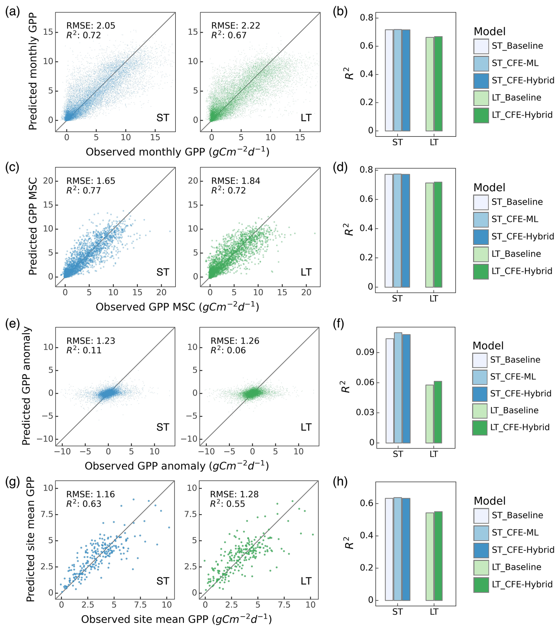
Figure 3 Machine learning model performance in predicting monthly GPP and its spatial and temporal variability. Only NT models are shown; DT results are provided in Fig. S1 in the Supplement. Scatter plots illustrate relationships between model predictions and observations for monthly GPP (a), mean seasonal cycle (MSC) (c), monthly anomaly (e), and cross-site variability (g) for ST_CFE-Hybrid_NT (left, blue) and LT_CFE-Hybrid_NT (right, green) models. Corresponding bar plots show the R² values for five NT model setups in predicting monthly GPP (b), MSC (d), monthly anomaly (f), and cross-site variability (h).

3.1.2 Performance by biome and climate zone

The predictive ability of our models varies across different PFTs and Köppen climate zones (Fig. 4). Here we present results from the CFE-Hybrid LT and ST models based on NT partitioning and note that patterns for the other CFE configurations and the DT GPP were similar (Figs. S3, S4, S5).

Model performance in terms of monthly GPP is highest for deciduous broadleaf forests, mixed forests, and evergreen needleleaf forests, with R² values above 0.76. Model accuracies are also high for savannas and grasslands, followed by croplands and wetlands, with R² values between 0.48 and 0.76. Model accuracies are lowest in evergreen broadleaf forests and shrublands, with R² values as low as 0.13. Across climate zones, models achieve the highest accuracy in predicting monthly GPP in cold climates with R² around 0.73–0.78, followed by tropics and temperate zones (R² ∼ 0.47–0.65). The short-term models have the lowest performance in polar regions with an R² value of around 0.37, and the long-term models have the lowest performance in arid regions with an R² value of 0.28. Interestingly, short-term and long-term models exhibit substantial differences in arid regions and shrublands marked by strong seasonality and interannual variabilities.

Model performance in terms of mean seasonal cycles across PFTs and climate zones follows patterns for monthly GPP, while disparities emerge for performance in terms of GPP anomaly and cross-site variability (Figs. 4, S3, S4, S5). The short-term model shows the highest predictive power in explaining monthly anomalies in arid regions with an R² value of 0.48, where savanna and shrublands sites are primarily located. Model performance in all other climate zones is significantly lower. The short-term model also demonstrates good performance in capturing anomalies in deciduous broadleaf forests. The long-term model's relative performance between PFTs and climate zones is mostly consistent with that of the short-term model, with lower accuracy in shrublands when compared to the short-term model.

Models demonstrate the highest accuracy in predicting cross-site variability in savannas, grasslands, evergreen needleleaf forests, and evergreen broadleaf forests (R² > 0.36) and the lowest accuracy in deciduous broadleaf forests, mixed forests, and croplands (R² < 0.1). The short-term model additionally shows good performance in shrublands and wetlands (R² > 0.36), whereas the long-term model fails to capture any variability for shrublands. In terms of climate zones, models are most successful at explaining the variabilities within tropical and cold climate zones (R² > 0.50), the short-term model has moderate performance in temperature and polar regions (R² ∼ 0.22), and the long-term model has low performance for both temperate and arid regions with R² values below 0.16.

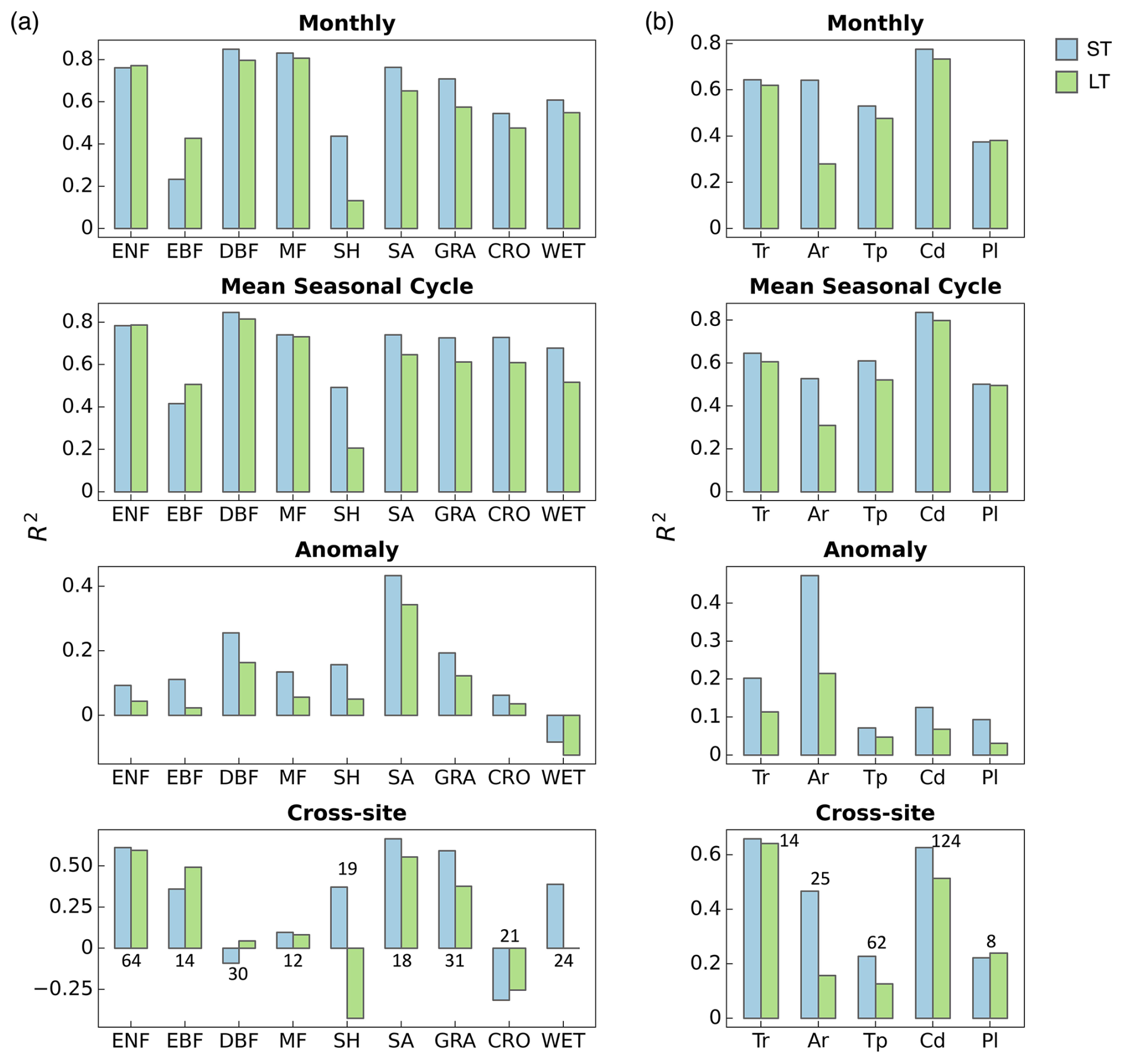
Figure 4 Performance of the ST_CFE-Hybrid_NT (blue) and LT_CFE-Hybrid_NT (green) models on GPP spatiotemporal estimation by plant functional types (a) and climate zones (b). The cross-site panels include the number of sites within each category. Color indicates short-term (ST) or long-term (LT) models. ENF: evergreen needleleaf forest; EBF: evergreen broadleaf forest; DBF: deciduous broadleaf forest; MF: mixed forest; SH: shrubland; SA: savanna; GRA: grassland; CRO: cropland; WET: wetland. Tr: tropical; Ar: arid; Tp: temperate; Cd: cold; Pl: polar. The performance of DT models is displayed in Fig. S3 in the Supplement.

3.1.3 Prediction of long-term trends

Eddy-covariance-derived GPP presents a substantial increasing trend across flux sites between 2002 and 2019 (Figs. 5a, S6a). The eddy covariance GPP from the night-time partitioning approach indicates an overall trend of 7.7 gC m⁻² yr⁻². In contrast, the ST_Baseline_NT model predicts a more modest overall trend of 3.1 gC m⁻² yr⁻² across the flux sites, primarily reflecting the indirect CO₂ effect manifested through the growth of LAI. Both the ST_CFE-ML_NT and ST_CFE-hybrid_NT models predict much higher trends of 5.4 and 4.5 gC m⁻² yr⁻² respectively, representing an improvement from the Baseline model by 74 % and 45 %, aligning more closely with eddy covariance observations. Similarly, the LT_CFE-Hybrid_NT model shows improved trend estimation compared with the LT_Baseline_NT model. All trends were statistically significant (p<0.05). Aggregated eddy covariance GPP experiences increasing trends of varied magnitudes across different climate zones and plant functional types (Figs. 5b, c; S6b, c). While the machine learning models generally do not fully capture the enhancement in GPP for most categories, the CFE-ML and/or CFE-hybrid models consistently outperform the Baseline models in both ST and LT setups. The CFE-ML setup predicts a higher trend than CFE-hybrid in most cases, suggesting that the data-driven approach captures more dynamics not represented in the theoretical model, which is based on conservative assumptions regarding the CO₂ sensitivity of photosynthesis (see Sect. 2.3.2 and Appendix B). The choice of remote sensing data (ST vs. LT configurations) does not lead to substantial differences in the predicted GPP trend. Most long-term flux sites (at least 10 years of records) with a significant trend experienced an increase in GPP, and the CFE-ML and/or CFE-hybrid models align closer to eddy covariance data than the Baseline models (Fig. S7). Additionally, we found a considerably higher trend in eddy covariance GPP measurements derived from the day-time versus night-time partitioning approach, potentially associated with uncertainties in GPP partitioning methods (Fig. S6). Yet, machine learning model predicted trends are not strongly affected by GPP partitioning methods.

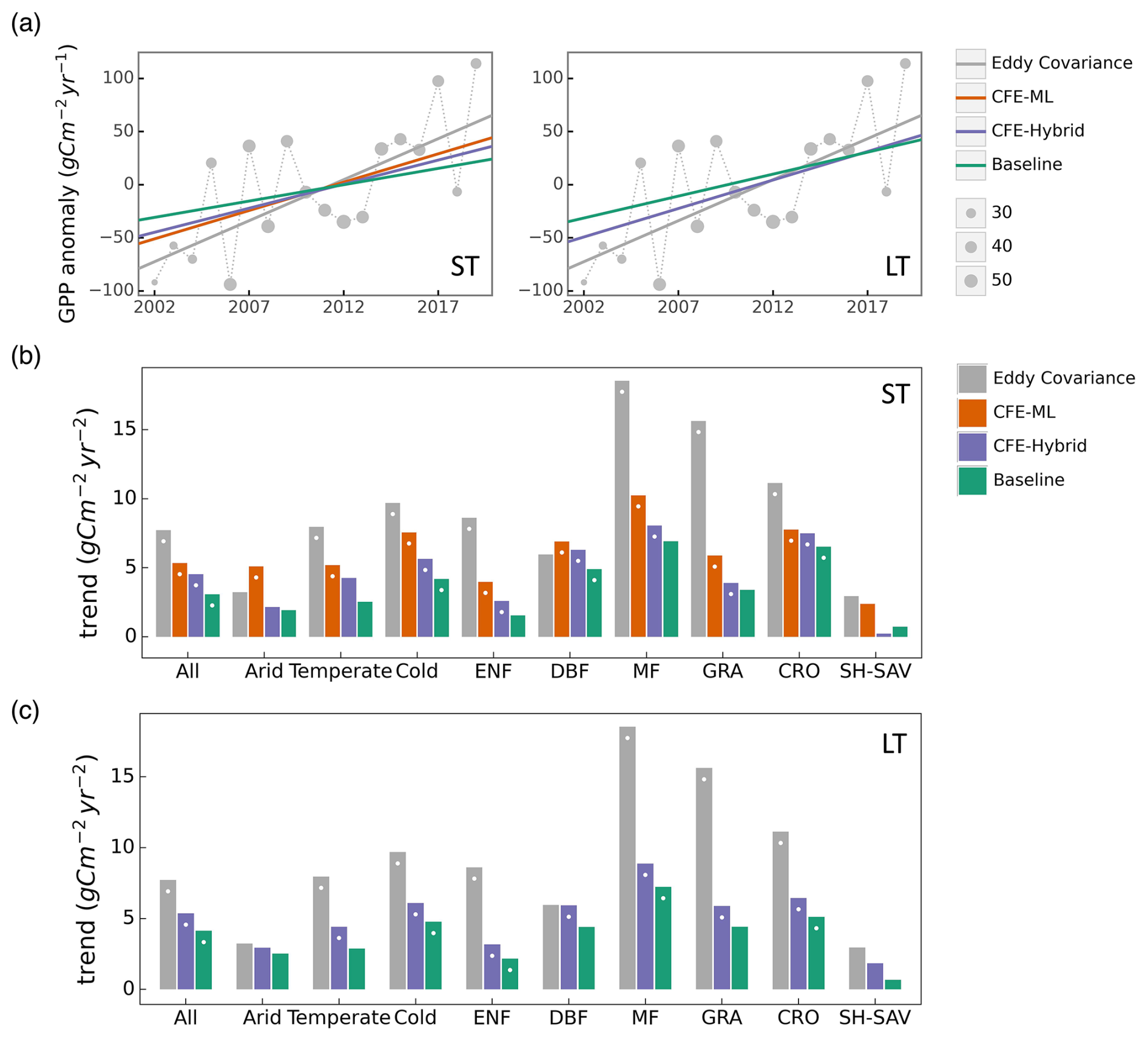
Figure 5 Comparison of observed and predicted GPP (from NT models only) trends across eddy covariance flux towers. (a) Aggregated annual GPP anomaly from 2002 to 2019 and trend lines from eddy covariance (EC) data, and three CFE model setups (short-term, night-time partitioning) for ST (left) and LT (right) models. The size of the gray circle markers is proportional to the number of sites. (b) Comparison of annual GPP trends from eddy covariance measurements and the short-term (ST) CEDAR-GPP model setups by plant functional types and climate zones. (c) Comparison of annual GPP trends from eddy covariance measurements and the long-term (LT) CEDAR-GPP model setups by plant functional types and climate zones. In (b) and (c), Categories with fewer than six sites, including Tropics and EBF, are not shown. White dots on the bars indicate statistically significant trends with p value < 0.1. Results for the DT models are shown in Fig. S3 of the Supplement.

The differences in estimated GPP trends between the Baseline and CFE models underscore the significant long-term GPP changes driven by the direct CO₂ effect. Using explainable machine learning approaches (ALE and SHAP) we further assessed the CFE-ML models for quantifying the direct CO₂ effect. Both approaches reveal a consistently positive influence of CO₂ on GPP, aligning with biophysical theories (Fig. S8). Compared to the effects from light (PAR) and vegetation structures (e.g., NIRv), the impacts of CO₂ are considerably smaller, which explains the minimal differences in overall model accuracy between the Baseline and CFE models.

Finally, we evaluated CEDAR-GPP using independent eddy covariance data (11 sites, Table S3) that was not involved in model training and obtained from the OzFlux FluxNet dataset (Ozflux, 2024). Among these sites, only two – AU-Cpr (Tropical) and AU-Stp (Aird) – with more than five years of records exhibit a GPP trend with p value less than 0.3. CEDAR-GPP shows strong consistency with the observed trend (Fig. S9). Additionally, CEDAR-GPP achieves reasonable accuracy in predicting monthly GPP (R² ∼ 0.73–0.75), mean seasonal cycle (R² ∼ 0.74–0.78), and monthly anomalies (R² ∼ 0.26–0.50; Table S4, Fig. S10), closely aligning with the cross-validation results.

3.2 Evaluation of GPP spatial and temporal dynamics

We compared CEDAR-GPP estimates with other upscaled or LUE-based datasets regarding the mean annual GPP (Sect. 3.2.1), GPP seasonality (Sect. 3.2.2), interannual variability (Sect. 3.2.3), and annual trends (Sect. 3.2.4). CEDAR-GPP model setups generally show similar patterns in mean annual GPP, seasonality, and interannual variability, therefore, in corresponding sections, we present the CFE-Hybrid model setups as representative examples for comparisons with other datasets, unless otherwise stated. Supplementary figures include comparisons involving CEDAR-GPP estimates from all model setups.

3.2.1 Mean annual GPP

Global patterns of mean annual GPP are generally consistent among CEDAR-GPP model setups, FLUXCOM, FLUXSAT, MODIS, and rEC-LUE, with few noticeable regional differences (Figs. 6, S11). Differences among CEDAR-GPP model setups are minimal and only evident between the NT and DT setups in the tropics (Figs. 6b–c, S11). CEDAR-GPP short-term datasets show highest consistency with FLUXSAT in terms of mean annual GPP magnitudes (2001–2018) and latitudinal variations, although FLUXSAT presents slightly higher GPP values in the tropics compared to CEDAR-GPP (Fig. 6b). Mean annual GPP magnitudes for FLUXCOM-RS006 and MODIS are lower globally than CEDAR-GPP and FLUXSAT, with the most pronounced differences observed in the tropical areas. Among the long-term datasets (CEDAR-GPP LT, FLUXCOM-ERA5, and rEC-LUE), mean annual GPP (1982–2018) exhibits greater disparities in the northern mid-latitudes than in the tropics and southern hemisphere (Fig. 6c). CEDAR-GPP aligns more closely with FLUXCOM-ERA5 than with rEC-LUE, with the latter showing lower annual mean GPP globally, particularly between 20° and 50° N.

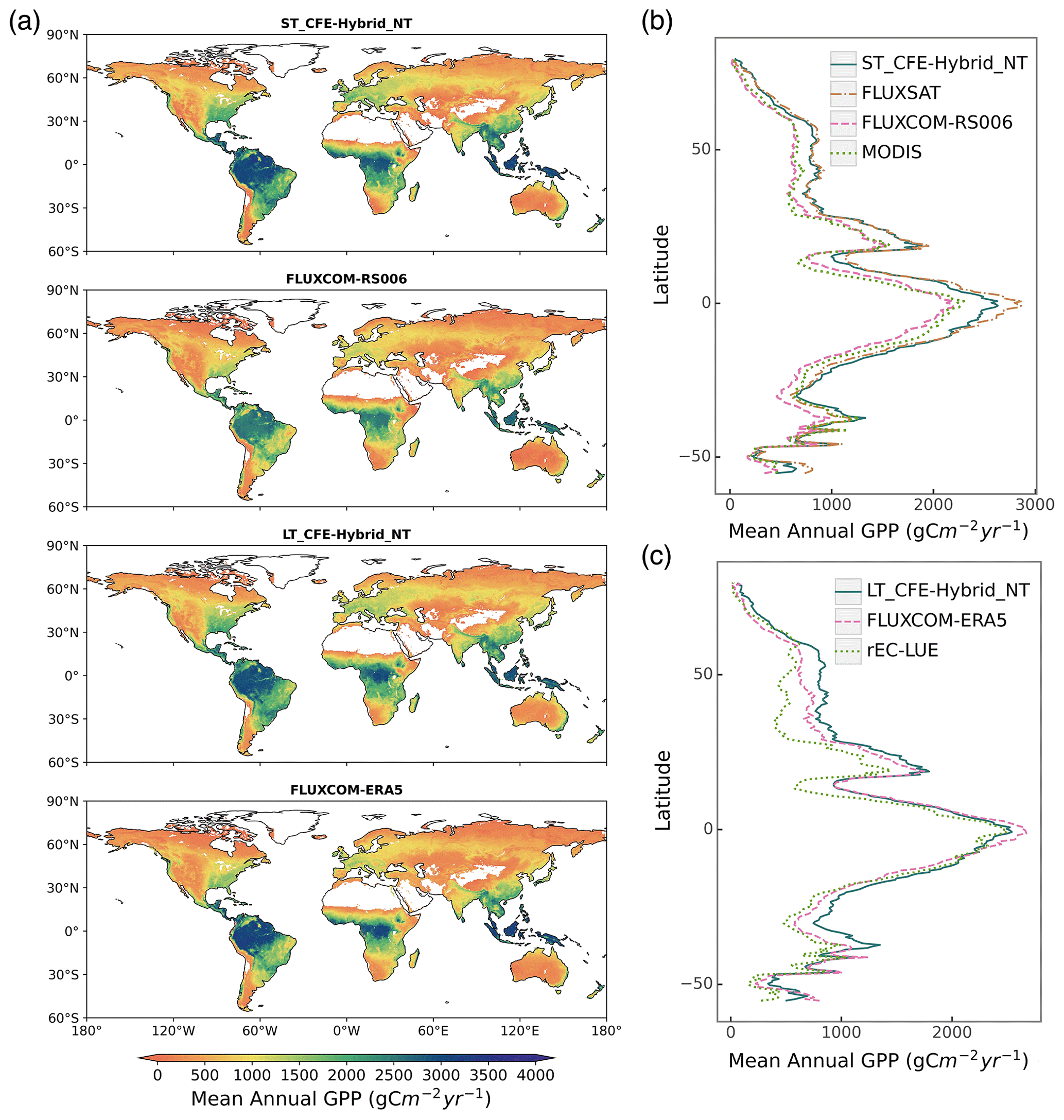
Figure 6 Global distributions of mean annual GPP from CEDAR-GPP and other machine learning upscaled and LUE-based reference datasets. (a) Global patterns of mean annual GPP from two short-term datasets including ST_CFE-Hybrid_NT, and FLUXCOM-RS006, and two long-term datasets including LT_CFE-Hybrid_NT, and FLUXCOM-ERA5. (b) Latitudinal distributions of mean annual GPP from short-term datasets (ST_CFE-Hybrid_NT, FLUXSAT, FLUXCOM-RS006, and MODIS). (c) Latitudinal distributions of mean annual GPP from long-term datasets (LT_CFE-Hybrid_NT, FLUXCOM-ERA5, and rEC-LUE). Mean annual GPP was computed between 2001 and 2018 for short-term datasets and between 1982 and 2018 for long-term datasets.

3.2.2 Seasonal variability

CEDAR-GPP agrees with other GPP datasets on seasonal variabilities (average between 2001 and 2018) at the global scale, characterized by a peak in GPP in July and a nadir between December and January (Figs. 7, S12). At the global scale, CEDAR-GPP is most closely aligned with FLUXSAT in GPP seasonal magnitude and amplitude, while both FLUXCOM and MODIS display a relatively less pronounced magnitude.

In boreal and temperate regions of the Northern Hemisphere, all datasets agree on seasonal GPP variation, with only minor variances in the magnitude of peak GPP. In Southern Hemisphere temperate regions, datasets demonstrate similar seasonality, though with greater variability in peak amplitudes compared to the Northern Hemisphere. The largest disparities are found in the South American tropical areas, where seasonal variation is less prominent. Here, FLUXSAT shows a distinct bi-modal pattern with peaks in March–April and September–October. CEDAR-GPP and FLUXCOM-ERA5 aligns with the second peak, but exhibit a less pronounced first peak. Interestingly, the DT setups of CEDAR-GPP show slightly higher peaks in March–April in this region (Fig. S13). MODIS, in contrast, indicates an inverse seasonal pattern, with a small peak from June to August. Across all regions, CEDAR-GPP's seasonality aligns more closely with FLUXSAT and FLUXCOM-ERA5 than with other datasets. Differences among the 10 CEDAR-GPP model setups are minimal, except for small variations in GPP magnitude in some tropical areas between NT and DT setups (Fig. S13).

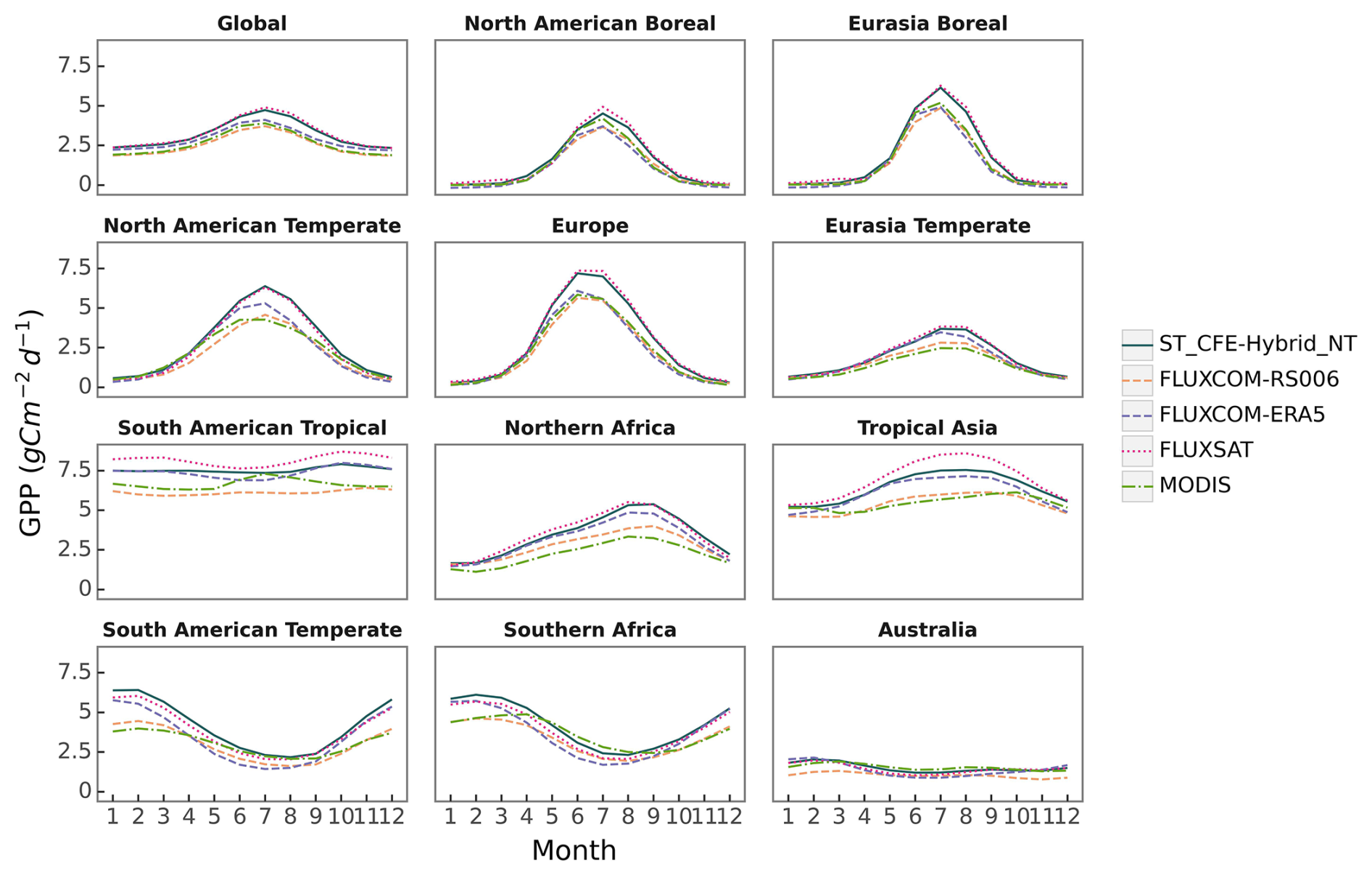
Figure 7 Comparison of global and regional GPP mean seasonal cycle between different datasets on a global scale. Monthly means were averaged from 2001 to 2018 for all datasets. Geographic boundaries of the 11 TransCom land regions were obtained from the CarbonTracker (CT2022) dataset and are shown in Fig. S18.

3.2.3 Interannual variability

We found distinct spatial patterns in GPP interannual variability between upscaled and LUE-based datasets and a high level of agreement within each category, with the exception of FLUXCOM-ERA5, which show minimal interannual variability globally (Figs. 8, S14). All datasets agree on the presence of GPP interannual variability hotspots in eastern and southern South America, central North America, southern Africa, and western Australia. These hotspots primarily correspond to arid and semi-arid areas characterized by grasslands, shrubs, and croplands (Fig. 9). CEDAR-GPP is highly consistent with FLUXSAT, and both datasets also display relatively high interannual variability in the dry subhumid areas of Europe, predominantly covered by croplands. FLUXCOM-RS006 mirrors the relative spatial patterns of CEDAR-GPP and FLUXSAT, albeit at lower magnitudes. The LUE-based datasets (MODIS and rEC-LUE) predict a much higher interannual variability than the upscaled datasets in the tropical areas, particularly in evergreen broadleaf forests and woody savannas (Figs. 8, 9). These datasets also depict slightly higher interannual variability for other types of forests, including evergreen needleleaf forests and deciduous broadleaf forests, compared to the upscaled datasets. The lack of interannual variability in FLUXCOM-ERA5 is attributable to the use of mean seasonal cycles of remotely sensed vegetation greenness indicators rather than their dynamic time series. Ten CEDAR-GPP model setups present consistent patterns in interannual variability, and differences are minimal (Fig. S14).

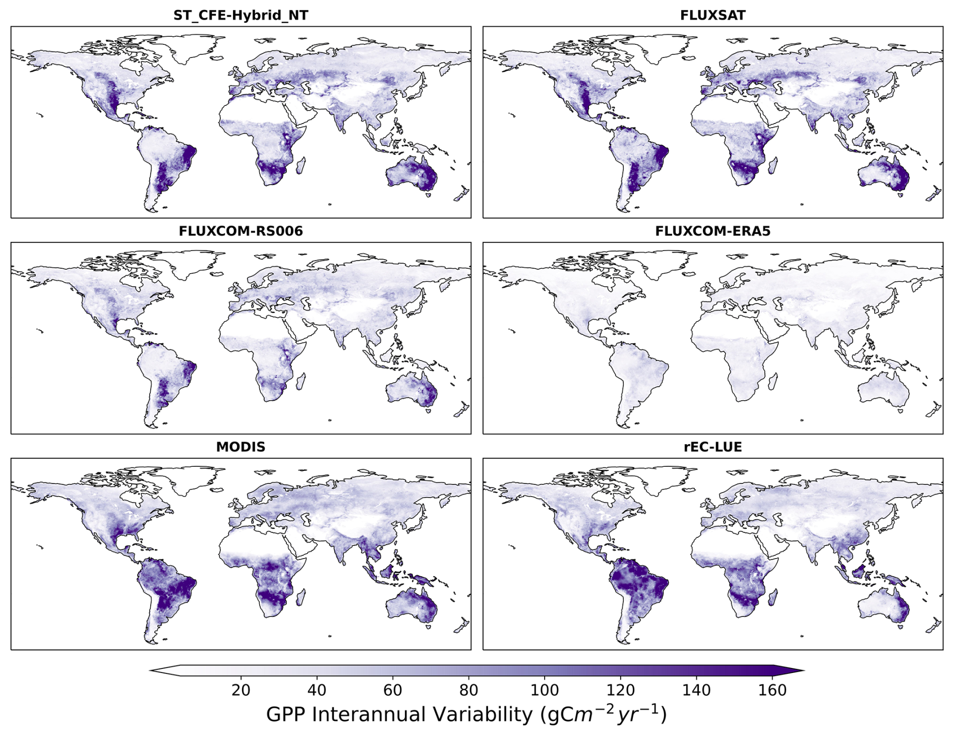
Figure 8 Spatial patterns of GPP interannual variability extracted over 2001 to 2018 for CEDAR-GPP (ST_CFE-Hybrid_NT), FLUXSAT, FLUXCOM-RS006, MODIS, FLUXCOM-ERA5, and rEC-LUE.

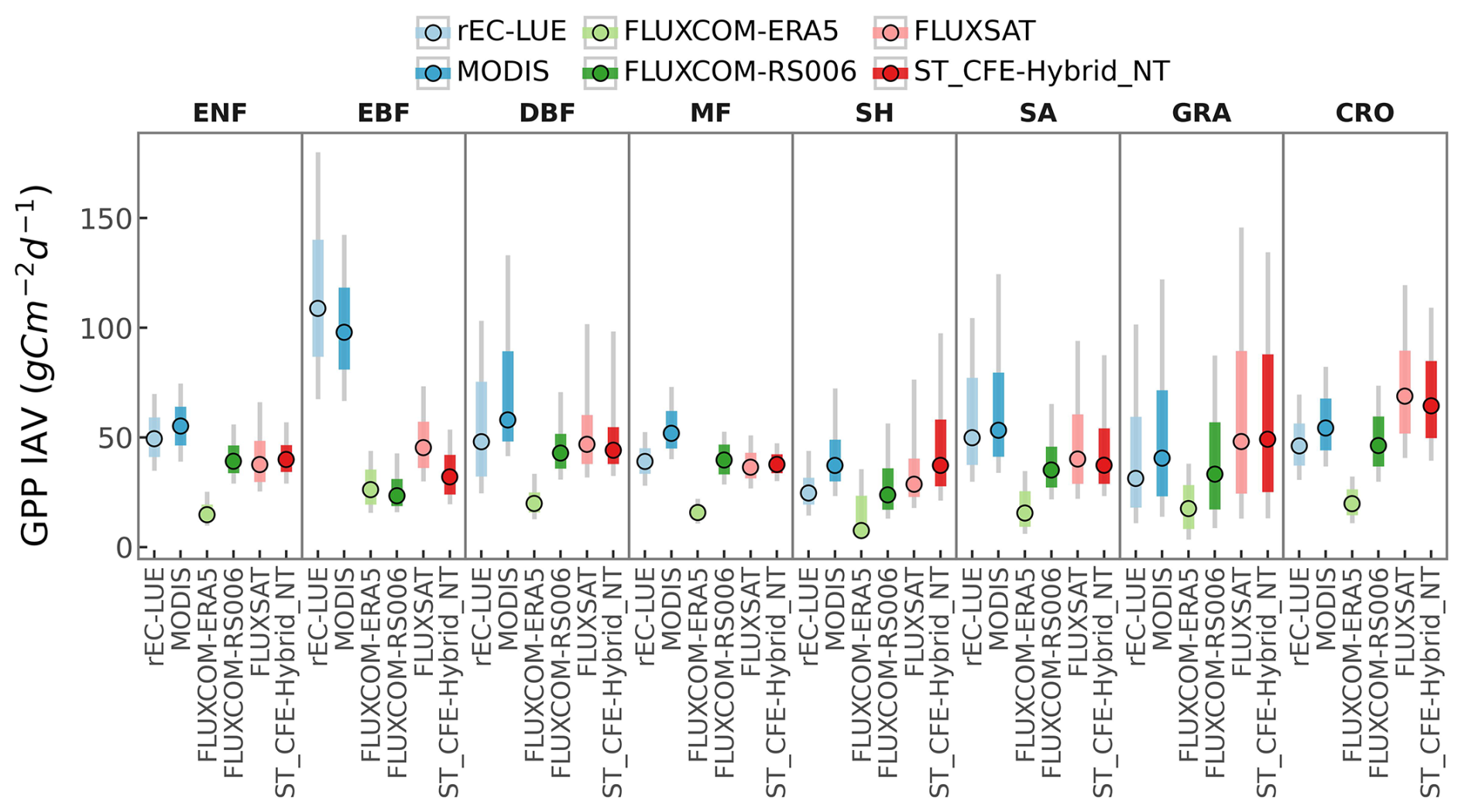
Figure 9 Comparison of GPP interannual variability (IAV) across global datasets by PFT. Colored dots represent the median IAV, thicker gray bars indicate the 25 % to 75 % percentiles of IAV distributions, and thinner gray bands show the 10 % to 90 % percentiles.

3.2.4 Trends

Differences in annual GPP trends among CEDAR-GPP model setups and other upscaled and LUE-based datasets mainly reflect the variability in the representation of CO₂ fertilization effects (Figs. 10, 11, S15). From 2001 to 2018, the CEDAR-GPP Baseline model setups show spatial variations in GPP trends consistent with the other upscaled datasets without direct CO₂ fertilization effects, including FLUXSAT and FLUXCOM-RSv006. In these datasets, substantial increases are seen in southeastern China and India, western Europe, and part of North and South America. These increases are largely associated with rising LAI due to land use changes and indirect CO₂ fertilization effects, as identified by previous studies (Chen et al., 2019; Zhu et al., 2016). Although MODIS, which also does not include a direct CO₂ fertilization effect, generally agrees with these increasing trends, it shows a declining GPP in the tropical Amazon and a stronger positive trend in central South America. After incorporating the direct CO₂ fertilization effects, both the CFE-Hybrid and CFE-ML setups predict positive trends in tropical forests, an observation absent in all other upscaled datasets. Furthermore, the CFE-Hybrid and CFE-ML models also reveal increasing GPP in temperate and boreal forests of North America and Eurasia. These patterns are also observed in BESS Vs and BEPS, while PML V2 presents minimal GPP changes in tropics and substantial reduction in Africa. Notably, all datasets agree on a pronounced GPP decrease in eastern Brazil and minimal changes in Australia.

From 2001 to 2018, a positive trend in global annual GPP is uniformly detected by all datasets, albeit with varying magnitudes (Figs. 12a, 13a, S16). The ST_Baseline_NT model predicts a GPP growth rate of 0.35 (±0.02) Pg C yr⁻², aligning with FLUXCOM-RS, but lower than FLUXSAT (0.51 Pg C yr⁻²) and MODIS (0.39 Pg C yr⁻²). The CFE-hybrid models estimate a notably faster GPP growth at 0.58 (±0.03) Pg C yr⁻², similar to BESS V2 and BEPS, both around 0.55 Pg C yr⁻². The CFE-ML models predict the highest trend, up to 0.76 (±0.15) Pg C yr⁻² from the ST_CFE-ML_NT model and 0.59 (±0.13) Pg C yr⁻² from the ST_CFE-ML_DT model. PML V2 displays a neutral trend of 0.08 Pg C yr⁻¹, and rEC-LU demonstrates an overall decline (0.20 Pg C yr⁻¹).

The LT_Baseline_NT model identifies increasing GPP trends in large areas of Europe, East and South Asia, and the Northern Amazon from 1982 to 2018 (Fig. 11). The pattern from the LT_CFE-Hybrid_NT model aligns closely with the LT_Baseline_NT model but exhibits a stronger positive trend in global tropical areas and Eurasian boreal forests. Spatial patterns of GPP trends from BESS V2 are consistent with LT_CFE-Hybrid_NT, though with considerably higher magnitudes. FLUXCOM-ERA5 shows overall negative trends in the tropics. rEC-LUE agrees with CEDAR-GPP in positive GPP trends in the extratropical areas, but predicts a pronounced negative trend in the tropics. At the global scale, all the CEDAR-GPP long-term models predict a positive global GPP trend (Figs. 12b, 13b). The LT_Baseline_ NT and LT_Baseline_DT models show a trend of 0.13 (±0.02) and 0.15 (±0.02) Pg C yr⁻² respectively, while the LT_CFE-Hybrid_NT and LT_CFE-Hybrid_DT models double these rates with 0.33 (±0.02) and 0.31 (±0.03) Pg C yr⁻² respectively. BESS V2 predicts the highest trend at 0.61 Pg C yr⁻². rEC-LUE shows a two-phased pattern with a strong increase in GPP from 1982 to 2000 (0.54 Pg C yr⁻²), followed by a decreasing trend after 2001 (−0.20 Pg C yr⁻²; Fig. S17). This results in an overall positive change at a rate comparable to that of the Baseline model. FLUXCOM-ERA5 exhibited a small negative trend.

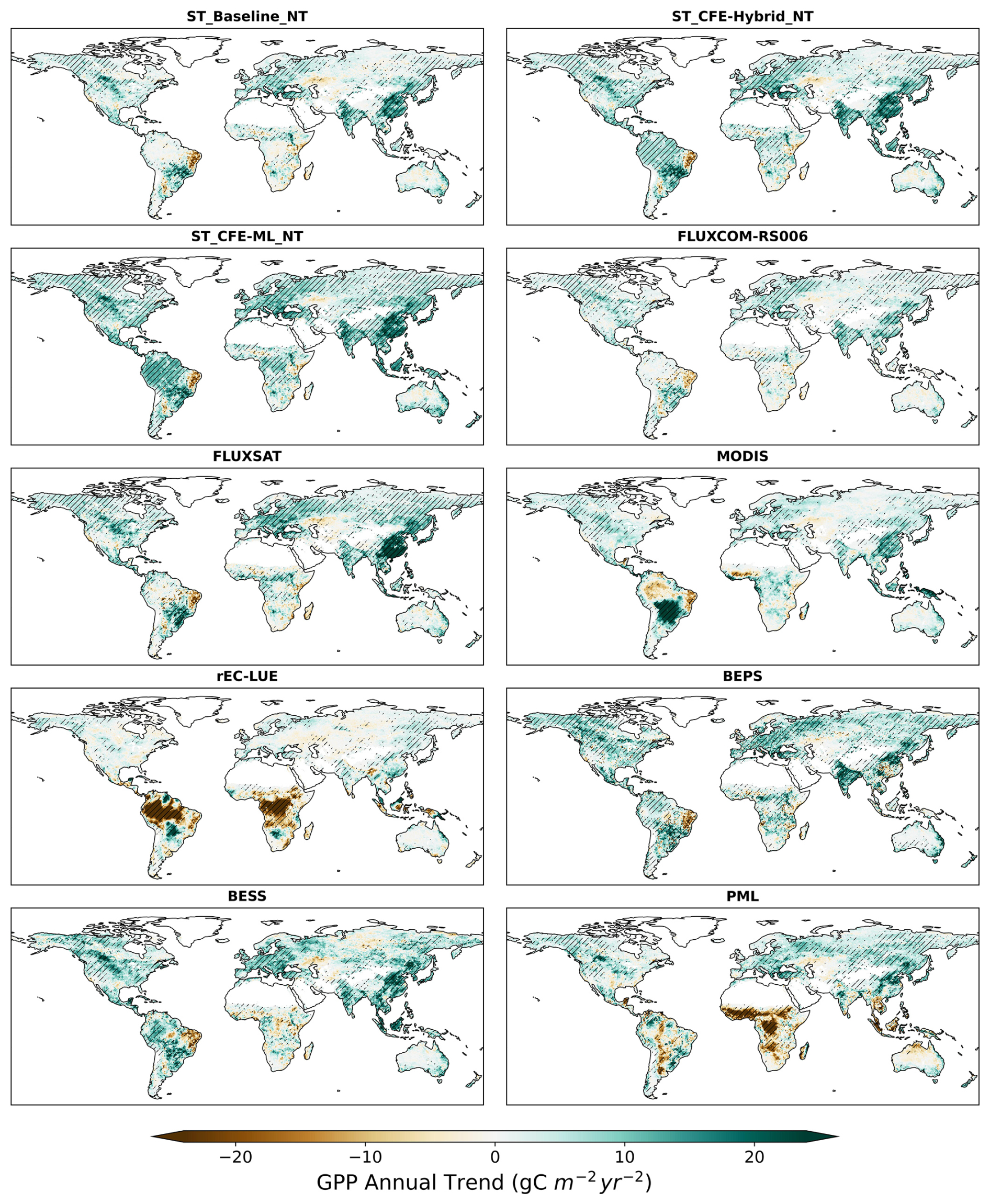
Figure 10 Annual GPP trend over 2001–2018 for short-term CEDAR-GPP, FLUXCOM-RS006, FLUXSAT, MODIS, BESS, BEPS, and PML datasets. Hatched areas indicate the GPP trend that is statistically significant at a p<0.05 level under the Mann–Kendall test.

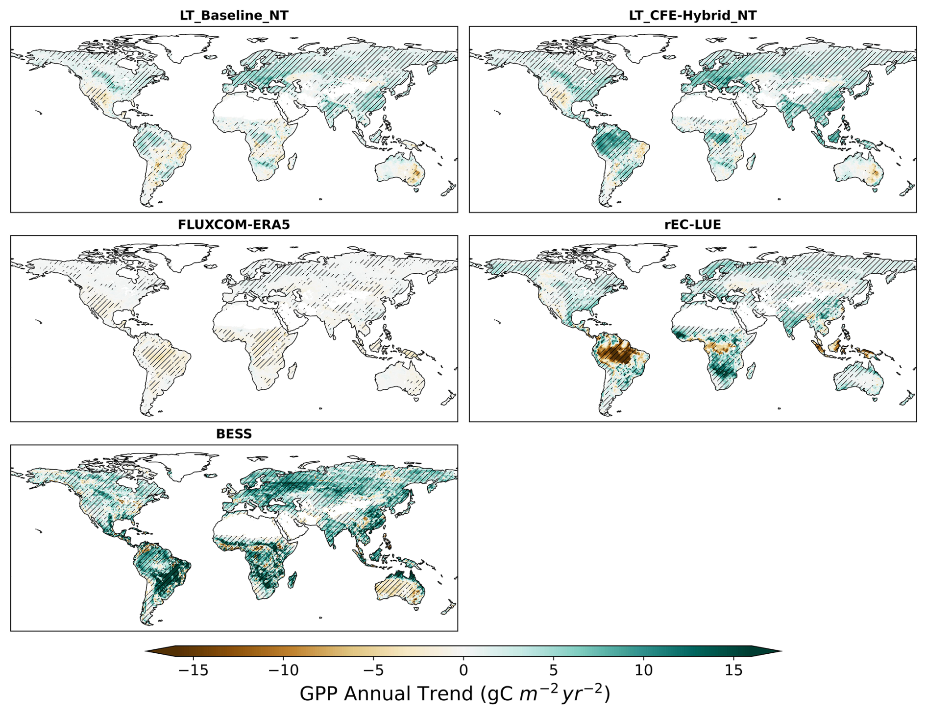
Figure 11 Annual GPP trend over 1982–2018 for long-term CEDAR-GPP, rEC-LUE, and BESS datasets. Hatched areas indicate the GPP trend that is statistically significant at a p<0.05 level under the Mann–Kendall test.

Figure 12 Global annual GPP variations (a) from 2001 to 2018 and (b) from 1982 to 2018.

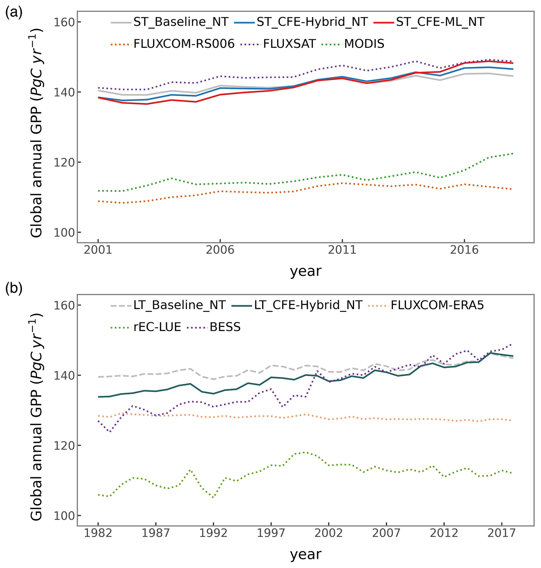
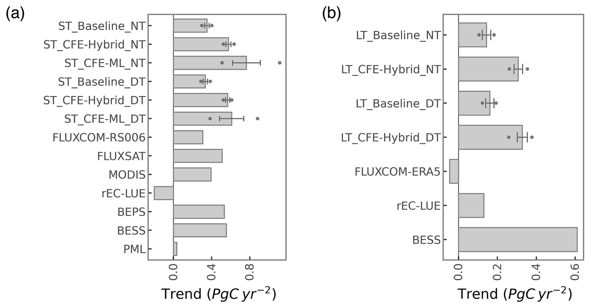
Figure 13 Global annual GPP trends for the (a) 2001 to 2018 and (b) 1982 to 2018 time periods. Error bars represent the 25 % to 75 % percentile from the model ensembles of CEDAR-GPP. Dots indicate the minimum and maximum from the model ensembles of CEDAR-GPP.

3.3 GPP estimation uncertainties

We analyzed the spread between the 30 model ensemble members in CEDAR-GPP as an indicator of uncertainties in GPP estimations. The spatial pattern of uncertainty in estimating annual mean GPP largely resembles that of the mean map (Figs. 14, 6a). The largest model spread is found in highly productive tropical forests, and this uncertainty decreases in temperate and cold areas (Fig. 14a). Tropical ecosystems, with a mean annual GPP between 1000 and 3500 Pg C yr⁻¹, only exhibit a 2 % and 6 % variation within the model ensemble (Fig. 14b). Ecosystems in the temperate and cold climates have a smaller annual GPP and proportionally small uncertainties of up to 6 %. However, ecosystems in arid and polar climates, despite their similarly low GPP, show higher model uncertainty, reaching 10 % to 40 % of the ensemble mean.

The estimation uncertainty of GPP trends is generally below 15 % to 20 % in the CEDAR-GPP datasets under the ST_Baseline and ST_CFE-Hybrid setups (Fig. 14c). However, in the ST_CFE-ML setup, the estimation increases substantially, with model spread reaching up to 40 % in tropical areas. Figure 15 (Fig. S19) further illustrates the trend uncertainties with the ensemble mean error range based on one standard deviation. Both the CFE-ML models show large discrepancies between the upper and lower uncertainty ranges, particularly within the tropics. Additionally, the long-term models also show a higher uncertainty compared to the short-term models.

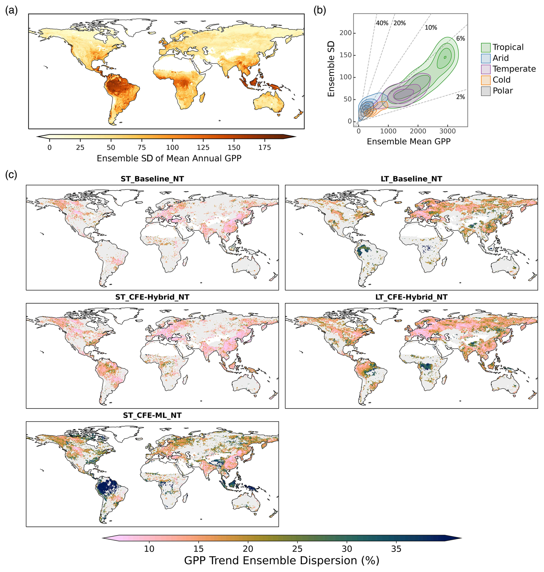
Figure 14 CEDAR-GPP estimation uncertainty derived from ensemble spread (standard deviation of 30 model predictions). (a) Spatial patterns of the absolute standard deviation from ensemble members in estimating the mean annual GPP from 2001 to 2018, using data from the ST_CFE-Hybrid_NT setup. (b) Relationships between ensemble standard deviation and ensemble mean in mean annual GPP. Colored contours denote clusters of Köppen climate zones. Dashed lines indicate the ratio between the ensemble standard deviation and the ensemble mean, with values shown in percentage. (c) Spatial patterns of model uncertainty in GPP long-term trend estimation. Only areas where 90 % of the ensemble members showed a statistically significant trend (p<0.05) are shown in the maps. The trend for the short-term datasets (left column) was computed between 2001 and 2018. The trend for the long-term datasets (right column) was computed between 1982 and 2018.

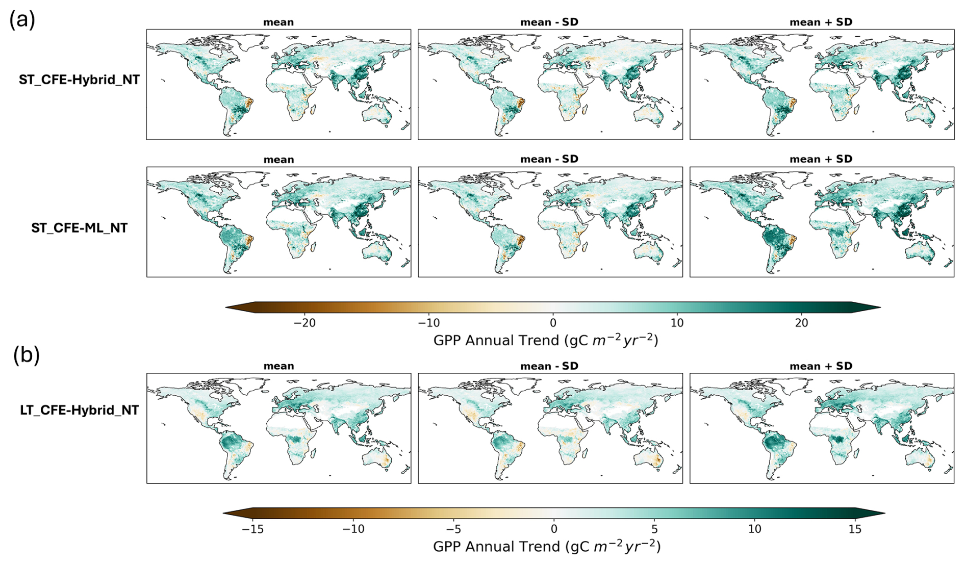
Figure 15 Maps of GPP trends and uncertainty range for CEDAR-GPP CFE datasets (NT only). The first column presents ensemble mean trends, the second column shows trends from the mean minus 1 standard deviation, and the third column indicates the trend from the mean plus 1 standard deviation. (a) Trends from the short-term (ST) datasets evaluated from 2001 to 2020. (b) Trends from the long-term (LT) dataset evaluated from 1982 to 2020. DT datasets were shown in Fig. S19.

4 Discussion

4.1 Reducing uncertainties in GPP upscaling

Here we examine the three predominant sources of uncertainties in machine learning upscaling of GPP: eddy covariance measurements, input datasets, and the machine learning model. We discuss strategies used in CEDAR-GPP to reduce the impacts of these uncertainties and highlight potential future research directions.

4.1.1 Eddy covariance data

Uncertainties associated with eddy covariance measurement and data processing can propagate through the upscaling process. CEDAR-GPP was produced using monthly aggregated eddy covariance data, where the impact of random errors in half-hourly measurements was minimized due to the temporal aggregation (Jung et al., 2020). Our stringent quality screening further reduced data processing uncertainties such as those associated with gap-filling. Yet, the discrepancy in GPP patterns between the CEDAR-GPP NT and DT setups is indicative of systematic biases linked to the partitioning approaches used to derive GPP from the NEE measurements (Keenan et al., 2019; Pastorello et al., 2020). Interestingly, the mean annual GPP from the DT setup is slightly higher than that from the NT setup (Fig. 6), and the DT setup also predicts a higher GPP trend in the long-term dataset (Fig. 13). While these discrepancies are relatively small compared to the predominant spatiotemporal patterns, the separate DT and NT setups in CEDAR-GPP offer an interesting quantification of the GPP partitioning uncertainties over space and time, providing insights for future methodology improvements.

The unbalanced spatial representativeness of the eddy covariance data constitutes a more significant source of uncertainty, as highlighted by previous studies (Jung et al., 2020; Tramontana et al., 2015). Effective generalization of machine learning models requires a substantial volume of training data that adequately represents and balances varied conditions. In CEDAR-GPP, this issue was mitigated with a large set of eddy covariance data (∼ 18 000 site-months) integrating FLUXNET2015 and two regional networks. However, data availability remains limited in critical carbon exchange hotspots such as tropics, subtropics, drylands, and boreal regions, as well as in mountainous areas (Fig. 1). Contrary to widespread perception that sparse training data leads to high upscaling uncertainties, our findings from the bootstrapped model spread indicates modest uncertainties in tropical areas relative to their high GPP magnitude (Fig. 14). This observation aligns with findings from the FLUXCOM product, revealing low extrapolation uncertainty in humid tropical regions (Jung et al., 2020). Nevertheless, to fully understand the upscaling uncertainty, it is essential to evaluate the generalization or extrapolation errors within the predictor space and consider the potential limitations of model structures (van der Horst et al., 2019; Villarreal and Vargas, 2021). Additionally, data limitations in mountainous areas and the absence of topology information in the predictor space in our models suggest potential uncertainties related to topographical effects on GPP (Hao et al., 2022; Xie et al., 2023).

Furthermore, our analysis suggests that the estimated global GPP magnitudes are related to the specific eddy covariance GPP data used in upscaling. Notably, global GPP magnitudes derived from CEDAR-GPP closely align with those from FLUXSAT, while the estimates from FLUXCOM were considerably lower (Figs. 6, 12). FLUXSAT used eddy covariance data from FLUXNET2015, which largely overlapped with that included in CEDAR-GPP (Joiner and Yoshida, 2020). FLUXCOM utilized data from the FLUXNET La Thuile set and CarboAfrica network, which consists of a distinct set of sites (Tramontana et al., 2016). The influence from the predictor datasets is minimal since all three datasets relied on MODIS-derived products. For a more in-depth evaluation of the impacts of flux site representativeness on upscaling, future research directions could include conducting synthetic experiments with simulations of ensembles of terrestrial biosphere models.

4.1.2 Input predictors and controlling factors

Upscaled GPP contains inherent uncertainties from the input predictors, including satellite and climate datasets. First, satellite remote sensing data contains noise resulting from Sun–Earth geometry, atmospheric conditions, soil background, and geolocation inaccuracies. The models or algorithms used for retrieving LAI, fAPAR, LST, and soil moisture also contain random errors and systematic biases specific to certain regions, biome types, or climatic conditions (Fang et al., 2019; Ma et al., 2019; Yan et al., 2016b). Moreover, satellite observations frequently contain missing values due to clouds, aerosols, snow, and algorithm failure, leading to both systematic and random uncertainties. In producing CEDAR-GPP, we mitigated these uncertainties through comprehensive preprocessing procedures. Our temporal gap-filling strategy exploits both the temporal dependency of vegetation status and long-term climatology to reduce biases from missing values. Temporal and spatial aggregation further reduces the remaining data gaps and random noises. Nevertheless, considerable uncertainties likely remain in satellite datasets impacting the upscaled estimations.

A potentially more impactful source of uncertainty is the mismatch between the footprint of the eddy covariance measurements and the coarse resolution of satellite observations. While flux towers typically have a footprint of ∼ 1 km² (Chu et al., 2021), satellite observations employed in CEDAR-GPP and most other upscaled datasets are at 5 km or lower resolution. Systematic and random errors could be introduced due to this mismatch, particularly in heterogenous biomes and areas with a mixture of vegetation and non-vegetated land covers. One mitigation strategy is to generate upscaled datasets at a higher spatial resolution (e.g., 500 m). Alternatively, models could be trained at a high resolution and applied to the coarse resolution to reduce computation and storage requirements (Dannenberg et al., 2023; Gaber et al., 2024). However, this approach does not address inherent scaling errors in coarse-resolution satellite images (Dong et al., 2023; Yan et al., 2016a).

Besides the quality of predictors, successful machine learning upscaling also requires a comprehensive set of features representing all controlling factors. For example, the lack of GPP interannual variabilities in FLUXCOM-ERA5 manifests the importance of incorporating dynamic vegetation signals from remote sensing in the upscaling framework. CEDAR-GPP used satellite observations from optical, thermal, and microwave systems, as well as climate variables thoroughly representing GPP dynamics. In particular, the inclusion of LST and soil moisture data provides important information about resource limitations and stress factors, which are crucial for certain biomes and/or under specific conditions (Green et al., 2022; Stocker et al., 2018, 2019). Dannenberg et al. (2023) showed that incorporating LST from MODIS and soil moisture from the SMAP satellite datasets substantially improved the machine learning estimation accuracy of GPP in North American drylands. Nevertheless, accurately capturing interannual anomalies remains challenging for certain biomes, such as evergreen needleleaf forest, cropland, and wetland (Fig. 4), as acknowledged by previous studies (Tramontana et al., 2016; Jung et al., 2020). High prediction uncertainties (Figs. 14, 15) in drylands also suggest the machine learning models did not sufficiently represent the mechanisms of water stress and drought responses. Potential improvement may be achieved by incorporating datasets related to agricultural management practices (crop type, cultivar, irrigation, fertilization; Xie et al., 2021), plant hydraulic and physiological properties (Liu et al., 2021), dynamic C₄ plant distributions (Luo et al., 2024), root and soil characteristics (Stocker et al., 2023), and topography (Xie et al., 2023).

4.1.3 Machine learning models and uncertainty quantification

The choice of machine learning models and their parameterization has been found to have a relatively minor impact on GPP upscaling uncertainties (Tramontana et al., 2015). CEDAR used the state-of-the-art boosting algorithm XGBoost, which provided high performance given the current data availability. Further reduction of model uncertainty will likely rely on additional information, such as increasing the number of eddy covariance sites or incorporating more high-quality predictors. Additionally, temporal dependency of carbon flux responses to atmospheric controls may also be exploited with specialized deep neural networks such as recurrent neural networks or transformers (Besnard et al., 2019; Ma and Liang, 2022).

A key challenge, however, is the quantification of uncertainties in machine learning upscaling (Reichstein et al., 2019). The limited availability of eddy covariance data hinders a comprehensive assessment of the extrapolation errors; consequently, metrics of predictive performance from cross-validation are inherently biased. CEDAR derived estimation uncertainty for each GPP prediction using a bootstrapping model ensemble, which naturally mimics the sampling bias associated with flux tower locations. Notably, the choice of input climate reanalysis datasets could also induce systematic differences in GPP spatial and temporal patterns (Tramontana et al., 2015). As a result, the FLUXCOM product generates model ensembles based on different reanalysis datasets to capture these uncertainties. Additionally, different satellite datasets of vegetation structural proxies, such as LAI, also exhibit significant discrepancies (Jiang et al., 2017). Thus, an ensemble approach combining site-level bootstrapping with multiple sources of input predictors could potentially provide a more comprehensive quantification of uncertainties. Furthermore, tree-based models do not generalize well to unseen conditions, and the uncertainty estimates derived from bootstrapping of XGBoost models may underrepresent actual biases stemming from limitations in training data representation. Future work may explore Bayesian neural networks, which provide uncertainty along with predictions and, at the same time, present high predictive power comparable to ensemble tree-based algorithms (Ma et al., 2021).

4.2 Long-term GPP changes and CO₂ fertilization effect

CEDAR-GPP was constructed using a comprehensive set of climate variables and multi-source satellite observations, thus encapsulating long-term GPP dynamics from both direct and indirect effects of climate controls. In particular, CEDAR-GPP included the direct CO₂ fertilization effect, which has been shown to dominate the increasing trend of global photosynthesis (Chen et al., 2022). Incorporating these effects substantially improved long-term trends of GPP from site to global scales (Figs. 5, 10, 11, 12, 13). CEDAR's CFE-Hybrid setup offers a conservative estimation of the direct CO₂ effects by simulating the CO₂ sensitivity of light-limited LUE for C₃ plants (Walker et al., 2021). However, the model does not account for the impacts of nutrient availability, which could potentially constrain CO₂ fertilization (Peñuelas et al., 2017; Reich et al., 2014; Terrer et al., 2019). Robust modeling of LUE responses to rising CO₂ under various environmental conditions remains challenging (Wang et al., 2017). Future work is needed to better understand how these factors affect the quantification of GPP and its long-term temporal variations.

The CFE-ML model adopted a data-driven approach to infer CO₂ effects directly from eddy covariance data. This strategy allows the model to potentially capture multiple physiological pathways of the CO₂ impact evidenced in the eddy covariance measurements, including the increases of biochemical rates and enhancements in water use efficiency (Keenan et al., 2013). The model detects a strong positive effect of CO₂ on eddy-covariance-measured GPP, consistent with previous studies based on process-based and statistical models (Chen et al., 2022; Fernández-Martínez et al., 2017; Ueyama et al., 2020). Moreover, spatial patterns of GPP trends derived from the CFE-ML model reflected a strong temperature dependency, aligning with the anticipated temperature sensitivity of photosynthetic biochemical processes (Keenan et al., 2023). Yet, the considerable ensemble spread in the CO₂ trends from the CFE-ML model and discrepancies between the CFE setups (Fig. 14) underscores a high level of uncertainty in the machine learning quantified CO₂ effects.

Several limitations should be noted regarding GPP trend estimation and validation. First, the CFE-ML model may not fully capture the intricate mechanisms of plant physiological responses to CO₂. For example, eddy covariance towers, especially long-term sites, are typically located in homogeneous and undisturbed ecosystems, not representative of the full diversity of ecosystems globally. Thus, interactions between CO₂ and natural or human-induced disturbance, as well as many other stresses, are likely underrepresented in the models. Ultimately, the model's capacity to robustly quantify CO₂ fertilization is constrained by the scope and diversity of the eddy covariance data. Additionally, the use of spatially invariant CO₂ data may not fully represent the actual CO₂ variations that plants experience across different environments.

Second, CO₂ effects inferred by the CFE-ML models may be confounded by other factors that correlate with CO₂ over time. Industrialization-induced nitrogen deposition could synergistically boost GPP alongside CO₂ (O'Sullivan et al., 2019). Technological and management improvements in agriculture that contribute to a global enhancement of crop photosynthesis (Zeng et al., 2014) might also be indirectly reflected in the model estimates. Moreover, interactions with the other input features that exhibit long-term trends, such as those induced by non-biological factors (e.g., sensor orbital drifts), also affect the CO₂ effects inference. Additionally, other factors that could lead to long-term GPP trends (e.g., forest aging, disturbances) might also be underrepresented in our models.

Finally, direct validation of GPP trends is limited, particularly in tropical regions, constrained by the availability of long-term records. Detecting and evaluating trends is challenging and typically requires long monitoring records (e.g., over 10 to 15 years), since long-term changes, such as those induced by CO₂, are very small relative to large interannual variations. Evaluating aggregated GPP trends across multiple sites presents an alternative approach; however, there were still insufficient sites in tropical and evergreen broadleaf forest areas to robustly validate our estimates for those ecosystems (Fig. 5). Partly due to data limitations, uncertainties in GPP estimated from bootstrapped samples are very high in tropical areas (Fig. 14). Thus, trend estimates in these areas should be interpreted in the context of associated uncertainties and limitations.

Our results also suggest that variations in the estimated GPP long-term trends from different products are largely related to the representation of CO₂ fertilization. Products that do not consider the direct CO₂ effect, including our Baseline models, FLUXSAT, FLUXCOM, and MODIS, show minimal long-term changes in tropical GPP, while the CEDAR CFE-ML and CFE-Hybrid models demonstrate significant GPP increases aligning with predictions from the terrestrial biosphere models (Anav et al., 2015). FLUXCOM-ERA5, not accounting for dynamic changes in vegetation structures and CO₂, does not capture either direct or indirect CO₂ fertilization, resulting in a slight negative GPP trend attributable to shifted climate patterns. Notably, rEC-LUE exhibits contrasting trends before and after circa 2000, primarily attributed to changes in vapor pressure deficit, PAR, and LAI, while the direct CO₂ fertilization effect remains consistent (Zheng et al., 2020). The CEDAR CFE-ML and CFE-Hybrid models align well with two process-based models forced with remote sensing data which consider direct CO₂ effects (BESS and BEPS). Nevertheless, considerable differences between CEDAR-GPP and other remote sensing products that include direct CO₂ effects (rEC-LUE and PML V2) warrant more in-depth investigations into long-term GPP responses to changes in atmospheric CO₂ and climate patterns.

Lastly, quantifications of GPP trends and their causes remain highly uncertain from site to global scales. Trend detection is often complicated by data noise and interannual variability, thus requiring long-term records which are limited in certain areas, biomes, and environmental conditions, such as tropics, polar regions, and wetlands, as well as ecosystems with regular or anthropogenic disturbances (Baldocchi et al., 2018; Zhan et al., 2022). Moreover, isolating the effect of CO₂ is challenging, as it is confounded by other factors such as forest regrowth, land cover change, and disturbances, which also significantly impacts long-term GPP variations. To this end, continued efforts in expanding ecosystem flux measurements and standardizing data processing present new opportunities to assess ecosystem productivity responses to changing climate conditions (Delwiche et al., 2024; Pastorello et al., 2020). Future research could also leverage novel machine learning techniques, such as knowledge-guided machine learning (Liu et al., 2024) and hybrid modeling that combines process-based and machine learning approaches (Kraft et al., 2022; Reichstein et al., 2019).

5 Data availability

The CEDAR-GPP product, comprising 10 GPP datasets, can be accessed at https://doi.org/10.5281/zenodo.8212706 (Kang et al., 2024). These datasets were generated at a spatial resolution of 0.05° and monthly time steps. Each dataset includes an ensemble mean GPP (“GPP_mean”) and an ensemble standard deviation (“GPP_std”). Data are formatted in netCDF with the following naming convention: “CEDAR-GPP_<version>_<model setup>_<YYYYMM>.nc”.

The CEDAR GPP product offers GPP estimates derived from 10 different models. Models are characterized by (1) temporal coverage, (2) configuration of CO₂ fertilization, and (3) GPP partitioning approach (Table 2). We provide a structured approach to selecting the most appropriate dataset for research or applications.

1. Study period considerations. The short-term (ST) setup is ideal for studies focusing on periods after 2000. These models are constructed using a broader range of explanatory predictors, offering higher precision and smaller random errors. The long-term (LT) datasets should be used for research assessing GPP dynamics over a longer time period (before 2001). It is important to note that trends from the ST and LT datasets are not directly comparable, as they were derived from different satellite remote sensing data.

2. CO₂ fertilization effect configurations. The CFE-Hybrid and CFE-ML setups are preferable when assessing temporal GPP dynamics, especially long-term trends. The CFE-Hybrid setup includes a hypothetical trend from the direct CO₂ effect, while CFE-ML is purely data-driven and does not make any specific assumption about the sensitivity of photosynthesis to CO₂. Averaging the CFE-Hybrid and CFE-ML estimates is acceptable, with the difference between them reflecting the uncertainty surrounding the direct CO₂ effect. Note that the Baseline setup should not be used to study long-term GPP dynamics, especially those induced by elevated CO₂. The Baseline setup may be useful to compare with other remote-sensing-derived GPP datasets that do not consider the direct CO₂ effect. Differences between these setups regarding mean GPP spatial patterns and seasonal and interannual variations are considered to be minor.

3. GPP partitioning methods. We recommend using the mean value derived from both the “NT” (night-time) and “DT” (day-time) data. The difference between these two provides insight into the uncertainties arising from the partitioning approaches used in GPP estimation from eddy covariance measurements.

Finally, like other upscaled or remote-sensing-based GPP datasets, CEDAR-GPP should not be regarded as “observations” but rather as model estimates informed by remote sensing and ground-based data. The extent of assumptions or structural constraints varies across such datasets. CEDAR-GPP, particularly in its CFE-Baseline and CFE-ML configurations, is entirely data-driven and incorporates no explicit assumptions regarding the biological and environmental processes underlying photosynthesis, apart from the generic assumptions inherent in machine learning models. Consequently, the usage and interpretation of this dataset should be carefully framed within the context of the input eddy covariance and environmental data as well as their limitations.

6 Code availability

The code for upscaling and generating global GPP datasets can be accessed at https://doi.org/10.5281/zenodo.8400968 (Kang, 2024).

7 Conclusions

We present the CEDAR-GPP product generated by upscaling global eddy covariance measurements with machine learning and a broad range of satellite and climate variables. CEDAR-GPP comprises four long-term datasets from 1982 to 2020 and six short-term datasets from 2001 to 2020. These datasets encompass three configurations regarding the incorporation of direct CO₂ fertilization effects and two partitioning approaches to derive GPP from eddy covariance data. The machine learning models of CEDAR-GPP demonstrated high capability in predicting monthly GPP, its seasonal cycles, and spatial variability within the global eddy covariance sites, with cross-validated R² between 0.56 to 0.79. Short-term model setups consistently outperformed long-term models due to considerably more and higher-quality information from multi-source satellite observations.

CEDAR-GPP advances satellite-based GPP estimations, as the first upscaled dataset that considered the direct biochemical effects of elevated atmospheric CO₂ on photosynthesis, which is responsible for an increasing land carbon sink over the past decades. We show that incorporating this effect in our CFE-ML and CFE-Hybrid models substantially improved the estimation of GPP trends at eddy covariance sites. Global patterns of long-term GPP trends in the CFE-ML setups show a strong temperature dependency consistent with biophysical theories. However, trend estimation and validation remain particularly challenging in data-scarce regions, such as the tropics, emphasizing the need for enhanced data availability and methodological advancements. Beyond trends, global spatial and temporal GPP patterns from CEDAR generally align with other satellite-based GPP datasets.

In conclusion, CEDAR-GPP, informed by global eddy covariance measurements and a broad range of multi-source remote sensing observations and climatic variables, offers a comprehensive representation of global GPP spatial and temporal dynamics over the past four decades. The different CO₂ fertilization configurations integrated in CEDAR-GPP offer new opportunities for understanding global ecosystem photosynthesis's response to increases in atmospheric CO₂ along different pathways over space and time. CEDAR-GPP is expected to serve as a valuable tool for benchmarking process-based modeling and constraining the global carbon cycle.

Appendix A

Table A1 List of eddy covariance sites.

Appendix B: CO₂ sensitivity function of light-use efficiency

In the CFE-Hybrid model, the direct CO₂ fertilization effect was prescribed onto machine learning-estimated GPP at a reference CO₂ level using a theoretical CO₂ sensitivity function of LUE. The sensitivity function, which describes the fractional change in LUE due to CO₂ relative to the reference period, is described below.

The light-use efficiency (LUE) model (Pei et al., 2022) of GPP states that

$$\begin{array}{}\text{(B1)}& \text{GPP}=\text{APAR}\times \text{LUE}=\text{PAR}\times \text{fAPAR}\times \text{LUE},\end{array}$$

where PAR is the photosynthetic active radiation, fAPAR is the fraction of PAR that the plant canopy has absorbed, and APAR is the absorbed PAR. Eco-evolutionary theory, specifically the optimal coordination hypothesis, predicts that the electron-transport-limited (light-limited) (A_j) and Rubisco-limited (A_c) rates of photosynthesis converge on the time scale of physiological acclimation, which is of the order of a few weeks (Harrison et al., 2021; Haxeltine and Prentice, 1996; Wang et al., 2017). Thus, at a monthly time scale, we assume that

$$\begin{array}{}\text{(B2)}& A=A_c=A_j,\end{array}$$

where A is the gross photosynthetic rate, here equivalent to GPP.

In the following, we derive our sensitivity function based on A_j, which has a smaller response to CO₂ than A_c, thus providing conservative estimates of the direct CO₂ fertilization effect (Walker et al., 2021). According to the Farquhar, von Caemmerer, and Berry (FvCB) model (Farquhar et al., 1980),

$$\begin{array}{}\text{(B3)}& A_j={\mathit{\phi }}_{\mathrm{0}}I{\displaystyle \frac{c_i-{\mathrm{\Gamma }}^{\ast }}{c_i+\mathrm{2}{\mathrm{\Gamma }}^{\ast }}},\end{array}$$

where φ₀ is the intrinsic quantum efficiency of photosynthesis, I is the absorbed PAR (I=APAR), c_i is the leaf-internal partial pressure of CO₂, and Γ^∗ is the photorespiratory compensation point that depends on temperature:

$$\begin{array}{}\text{(B4)}& {\mathrm{\Gamma }}^{\ast }=r_{\mathrm{25}}{e}^{\frac{\mathrm{\Delta }H(T-\mathrm{298.15})}{\mathrm{298.15}}RT},\end{array}$$

where r₂₅=4.22 Pa is the photorespiratory point at 25 °C, ΔH is the activation energy (37.83×10³ J mol⁻¹), T is the air temperature in Kelvin, and R is the molar gas constant (8.314 J mol⁻¹ K⁻¹). We denote the atmospheric CO₂ concentration as c_a, and χ is the ratio of leaf internal and external CO₂, so

$$\begin{array}{}\text{(B5)}& c_i=\mathit{\chi }{c}_{\mathrm{a}}.\end{array}$$

Combining Eqs. (B1), (B3), and (B5), and assuming Eq. (B2), LUE can be written as

$$\begin{array}{}\text{(B6)}& \mathrm{LUE}={\mathit{\phi }}_{\mathrm{0}}{\displaystyle \frac{c_i-{\mathrm{\Gamma }}^{\ast }}{c_i+\mathrm{2}{\mathrm{\Gamma }}^{\ast }}}={\mathit{\phi }}_{\mathrm{0}}{\displaystyle \frac{\mathit{\chi }{c}_{\mathrm{a}}-{\mathrm{\Gamma }}^{\ast }}{\mathit{\chi }{c}_{\mathrm{a}}+\mathrm{2}{\mathrm{\Gamma }}^{\ast }}}.\end{array}$$

We can therefore show that under constant absorbed light (I or APAR), the sensitivity of GPP to CO₂ is proportional to that of LUE,

$$\begin{array}{}\text{(B7)}& {\displaystyle \frac{\partial \mathrm{GPP}}{\partial c_{\mathrm{a}}}}={\displaystyle \frac{\partial {\mathit{\phi }}_{\mathrm{0}}I\frac{\mathit{\chi }{c}_{\mathrm{a}}-{\mathrm{\Gamma }}^{\ast }}{\mathit{\chi }{c}_{\mathrm{a}}+\mathrm{2}{\mathrm{\Gamma }}^{\ast }}}{\partial c_{\mathrm{a}}}}=I{\displaystyle \frac{\partial \mathrm{LUE}}{\partial c_{\mathrm{a}}}}.\end{array}$$

Thus, from Eq. (B7) we can express the actual GPP at time t and a CO₂ level $c_{\mathrm{a}}^t$ as the product of a reference GPP with a CO₂ level $c_{\mathrm{a}}^{\mathrm{0}}$ and the ratio between actual and reference LUE (B8–9). We denote the actual GPP as time t as ${\mathrm{GPP}}_{c_{\mathrm{a}}=c_{\mathrm{a}}^t}^t$, and the reference GPP at time t as ${\mathrm{GPP}}_{c_{\mathrm{a}}=c_{\mathrm{a}}^{\mathrm{0}}}^t$.

$$\begin{array}{}\text{(B8)}& {\displaystyle \frac{{\mathrm{GPP}}_{c_{\mathrm{a}}=c_{\mathrm{a}}^t}^t}{{\mathrm{GPP}}_{c_{\mathrm{a}}=c_{\mathrm{a}}^{\mathrm{0}}}^t}}={\displaystyle \frac{{\mathrm{LUE}}_{c_{\mathrm{a}}=c_{\mathrm{a}}^t}^t}{{\mathrm{LUE}}_{c_{\mathrm{a}}=c_{\mathrm{a}}^{\mathrm{0}}}^t}}={\displaystyle \frac{\frac{\mathit{\chi }{c}_{\mathrm{a}}^t-{\mathrm{\Gamma }}^{\ast }}{\mathit{\chi }{c}_{\mathrm{a}}^t+\mathrm{2}{\mathrm{\Gamma }}^{\ast }}}{\frac{\mathit{\chi }{c}_{\mathrm{a}}^{\mathrm{0}}-{\mathrm{\Gamma }}^{\ast }}{\mathit{\chi }{c}_{\mathrm{a}}^{\mathrm{0}}+\mathrm{2}{\mathrm{\Gamma }}^{\ast }}}}={\displaystyle \frac{{\mathit{\varphi }}_{{\mathrm{CO}}_{\mathrm{2}}}^t}{{\mathit{\varphi }}_{{\mathrm{CO}}_{\mathrm{2}}}^{t_{\mathrm{0}}}}}\text{(B9)}& {\displaystyle }{\mathrm{GPP}}_{c_{\mathrm{a}}=c_{\mathrm{a}}^t}^t={\mathrm{GPP}}_{c_{\mathrm{a}}=c_{\mathrm{a}}^{\mathrm{0}}}^t\times {\displaystyle \frac{{\mathit{\varphi }}_{{\mathrm{CO}}_{\mathrm{2}}}^t}{{\mathit{\varphi }}_{{\mathrm{CO}}_{\mathrm{2}}}^{t_{\mathrm{0}}}}}\end{array}$$

The reference GPP represents the GPP value at time t if the CO₂ were at the level of a reference level, while all other factors, such as PAR, fAPAR, temperature, and other environmental controls, remain unchanged. Here, the CO₂ impacts on LUE depend on atmospheric CO₂ (c_a), χ, and air temperature. We fixed χ to the global long-term average value of 0.7 typical for C₃ plants (Prentice et al., 2014; Wang et al., 2017). We further tested a dynamic model that quantified χ as a function of air temperature and vapor pressure deficit following an eco-evolutionary theory across global flux sites (Keenan et al., 2023). The estimated χ had a mean and median of 0.7 and a standard deviation of 0.04 (Fig. S20a). Differences in the direct CO₂ effect between the dynamic and fixed χ approaches were minimal, with an R² of 0.99 and a slope of 0.99 from a least squares linear regression line (Fig. S20b). GPP trends across flux towers were also highly consistent between the two approaches, with a difference of less than 0.1 gC m⁻² yr⁻² (Fig. S20b, c). Since these results indicated that χ is relatively stable, we used the fixed χ approach to produce the CEDAR-GPP dataset.

In the CFE-Hybrid model, we estimated the reference GPP by fixing the CO₂ at the level of the year 2001 while keeping all other variables dynamic in the CFE-ML model. Then the actual GPP can be estimated following Eq. (B9). Fixing CO₂ values to the 2001 level, the start year of eddy covariance data used in model training, essentially removed the effects of CO₂ inferred by the CFE-ML model.