A continual-learning-based multilayer perceptron for improved reconstruction of three-dimensional nitrate concentrations

Nitrate plays a crucial role in marine ecosystems, as it influences primary productivity. Despite its ecological significance, accurately mapping its three-dimensional (3D) concentration on a large scale remains a considerable challenge due to the inherent limitations of existing methodologies. To address this issue, this study proposes a continual-learning-based multilayer perceptron (MLP) model to reconstruct the 3D ocean nitrate concentrations above 2000 m depth over the pan-European coast. The continual-learning strategy enhances the model generalization by integrating knowledge from Copernicus Marine Environmental Monitoring Service (CMEMS) nitrate data, effectively overcoming the spatial limitations of Biogeochemical Argo (BGC-Argo) observations in comprehensive nitrate characterization. The proposed approach integrates the advantages of extensive spatial remote sensing observations, the precision of BGC-Argo measurements, and the broad knowledge from simulated nitrate datasets, exploiting the capacity of neural networks to model their nonlinear relationships between multisource sea surface environmental variables and subsurface nitrates. The model achieves excellent performance in profile cross-validation (R²=0.98, RMSE = 0.592 µmol kg⁻¹) and maintains robustness across diverse 3D validation scenarios, suggesting its effectiveness in filling observational gaps and reconstructing the 3D nitrate field. Then, the spatiotemporal distribution of the reconstructed 3D nitrate field from 2010 to 2023 reveals a spatial distribution pattern, an interannual upward trend, and the degree of consistency in vertical variation. The contributions of all 22 input features to the model's estimation were quantified using Shapley additive explanation values. This study reveals the potential of the proposed approach to overcome observational limitations and provide further insights into the 3D ocean condition. The reconstructed 3D nitrate dataset is freely available at https://doi.org/10.5281/zenodo.14010813 (Yu et al., 2024).

1 Introduction

In the last decade, the global oceans have absorbed approximately 25 % of the anthropogenic carbon dioxide (CO₂) of the atmosphere, playing a crucial role in mitigating climate change impacts (Friedlingstein et al., 2020). However, oceanic changes such as warming and eutrophication may alter this role, leading to complex effects on marine ecosystems and climate. As the primary limiting nutrient in the upper ocean, nitrate is pivotal in regulating primary productivity, especially new productivity (Bristow et al., 2017; Chen et al., 2023). This could constitute long-term absorption of CO₂ from the surface to the ocean interior (Eppley and Peterson, 1979; Gregg et al., 2003; Joo et al., 2016; Rafter et al., 2017). Thus, comprehensive understanding of the temporal and spatial distributions of ocean nitrate is indispensable for conducting research on marine ecology and the environment.

Most biogeochemical data are collected in situ via coastal surveillance, oceanographic cruises, offshore platforms, or autonomous instruments, such as the Global Ocean Data Analysis Project version 2 (GLODAPv2) database and Biogeochemical Argo (BGC-Argo) (Claustre et al., 2020; Lavigne et al., 2015; Nittis et al., 2007). However, traditional in situ measurements alone cannot provide large-scale and continuous nitrate data. In contrast, remote sensing offers a promising alternative for estimating nitrate due to its broad spatial coverage, temporal consistency, and cost-effectiveness (Chang et al., 2013; Pan et al., 2018). Previous research has successfully utilized it to retrieve water nutrients (Ansper and Alikas, 2019; Du et al., 2020; Mortula et al., 2020; Yu et al., 2016). Machine learning (ML) technologies have also been employed for nutrient concentration retrieval (Huang et al., 2021; Lv et al., 2020; Qun'ou et al., 2021).

Optical satellites face challenges in nitrate retrieval due to the lack of distinctive nitrate signals (Chen et al., 2023; Sathyendranath et al., 1991). Previous studies have demonstrated a strong empirical correlation between sea surface nitrate (SSN) and certain measurable seawater parameters (Goes et al., 2000; Joo et al., 2018; Kamykowski et al., 2002; Silió-Calzada et al., 2008; Switzer et al., 2003). Physical processes, biological activity, and chemical reactions like nitrification are commonly recognized as the three principal processes in regulating ocean nitrate (Goes et al., 2000, 1999; Kudela and Dugdale, 2000; Pan et al., 2018). Cold and nitrate-rich water is transported to the euphotic layer through physical processes, including upwelling and convective mixing in winter, enriching SSN while decreasing sea surface temperature (SST) (Kudela and Dugdale, 2000; Pan et al., 2018). Phytoplankton growth consumes nitrate and converts it into organic matter, reducing SSN while increasing the chlorophyll (Chl) concentration (Goes et al., 2000, 1999). Therefore, various physical and biogeochemical characteristics were frequently utilized as features to establish empirical connections with SSN. The conventional method for nitrate retrieval typically relies solely on SST for linear regression, given its negative relationship with SSN (Sarangi and Devi, 2017; Switzer et al., 2003). Nevertheless, the correlation between SST and SSN is subject to significant geographical and temporal variation that is influenced by differing environmental conditions across regions (Goes et al., 1999; Silió-Calzada et al., 2008). Goes et al. (1999) found that incorporating Chl a alongside SST noticeably improves the accuracy of SSN retrieval compared to using SST in isolation. Additionally, colored dissolved organic matter (CDOM) is a feasible candidate for oceans with considerable river inflow (Pan et al., 2018).

One primary limitation of remote sensing retrieval is the challenge of accurately monitoring subsurface environmental parameters (Akbari et al., 2017; Ali et al., 2004). While in situ data provide precise measurements of local vertical conditions, they are inadequate for characterizing ecosystem processes occurring at the extensive temporal and spatial scales involved (Von Schuckmann et al., 2019). Accurate three-dimensional (3D) data acquisition for key variables over extensive scales is necessary for a deeper understanding of marine ecosystems (Rossi et al., 2021). To address this issue, various methods such as modeling ecosystems and ocean dynamics have been explored to estimate biogeochemical variables, with some being widely applied (Baretta et al., 1995; Bruggeman and Bolding, 2014; Holt et al., 2012; Kay and Butenschön, 2018). However, these methods require a thorough representation of physical and biological processes with highly nonlinear dynamics. While they can simulate environmental parameters and their distribution mechanisms, they might not always achieve the accuracy needed for specific applications (Storto et al., 2019; Tian et al., 2022).

In contrast, synergizing the extensive coverage of satellite data with the high precision of in situ data represents an effective approach, enabling the frequent characterization of the ocean's vertical structure across an expanded spatial scope (Buongiorno Nardelli, 2020; Tian et al., 2022; Gao et al., 2024; Zhou and Zhang, 2023). Empirical models were widely used to extrapolate important ocean variables from the surface to deeper layers (Morel and Berthon, 1989; Uitz et al., 2006), but they were vulnerable to inaccurate estimates due to the intricacy and nonlinearity, particularly in locations with irregular vertical stratification and small-scale phenomena (Sammartino et al., 2020). Recent advancements in neural network (NN) technology have yielded promising results in addressing this issue (Asdar et al., 2024). For instance, Richardson et al. (2002) pioneered the use of an unsupervised NN for vertical chlorophyll reconstruction. Supervised NNs are capable of fitting nonlinear relationships between sea surface environmental variables and deep-sea conditions and have been applied successfully to the estimation or prediction of various subsurface ocean parameters such as temperature, salinity (Buongiorno Nardelli, 2020; Qi et al., 2022; Smith et al., 2023; Su et al., 2021), and density (Su et al., 2024). Additional studies have supplemented sea surface parameters with reanalysis or profile data to reconstruct more subsurface parameters (Hu et al., 2023; Tian et al., 2022; Zhou and Zhang, 2023). However, due to the complex mechanisms and heterogeneous distribution of nitrate (Webb, 2021), its 3D reconstruction was not developed as effectively as parameters like temperature, particularly as the need for concurrent vertical observations of additional variables persists. Wang et al. (2023) employed a regionalized deep neural network (DNN) to estimate nitrate concentration in the northwestern Pacific Ocean. Similar supervised techniques based on a multilayer perceptron (MLP) have been utilized to rebuild water column bio-optical and biogeochemical variables using remote sensing and BGC-Argo data (Fourrier et al., 2020; Sauzède et al., 2017). A Bayesian strategy was proposed to supplement in situ data by inferring vertical profiles of unmeasured variables (Bittig et al., 2018). Yang et al. (2024) successfully reconstructed the 3D nitrate structure of the Indian Ocean from surface data using two advanced artificial intelligence networks. However, relying on simulated data rather than actual observations for training cannot overcome the inherent uncertainties, which may limit the model's applicability in real ocean environments.

In this study, we develop an MLP to accurately reconstruct the 3D nitrate concentration in the upper 2000 m of the ocean, addressing the aforementioned challenges. Including vertical profile variables in the features might introduce potential uncertainty and limit the expansion of the estimation range, so input features are based exclusively on sea surface environmental variables. The model employs a continual-learning strategy (Kirkpatrick et al., 2017), initially pre-training on simulated nitrate data to boost its generalization capabilities. The 3D nitrate field of the pan-European ocean from 2010 to 2023 is reconstructed based on this model and reveals the spatiotemporal distribution and interannual variations. Additionally, the contribution of each feature to the model estimates is calculated using Shapley values (Lundberg and Lee, 2017; Shapley, 1988), quantifying the effectiveness of the features.

2 Material and methods

2.1 Study area

The study area extends from 30° W to 37° E in latitude and from 30 to 65° N in longitude, covering the Mediterranean Sea (MED) and a portion of the northeastern Atlantic (NEA). This area is considered to be coastal in the pan-European domain, as shown in Fig. 1. It represents a critical zone for biogeochemical studies due to its extensive BGC-Argo observations and its unique position as one of the most data-rich coastal-proximate areas, where some of the continental shelf seas within this domain exhibit disproportionately high primary productivity and play a fundamental role in regulating oceanic biogeochemical cycles (Longhurst et al., 1995; Holt et al., 2009; Smith and Hollibaugh, 1993).

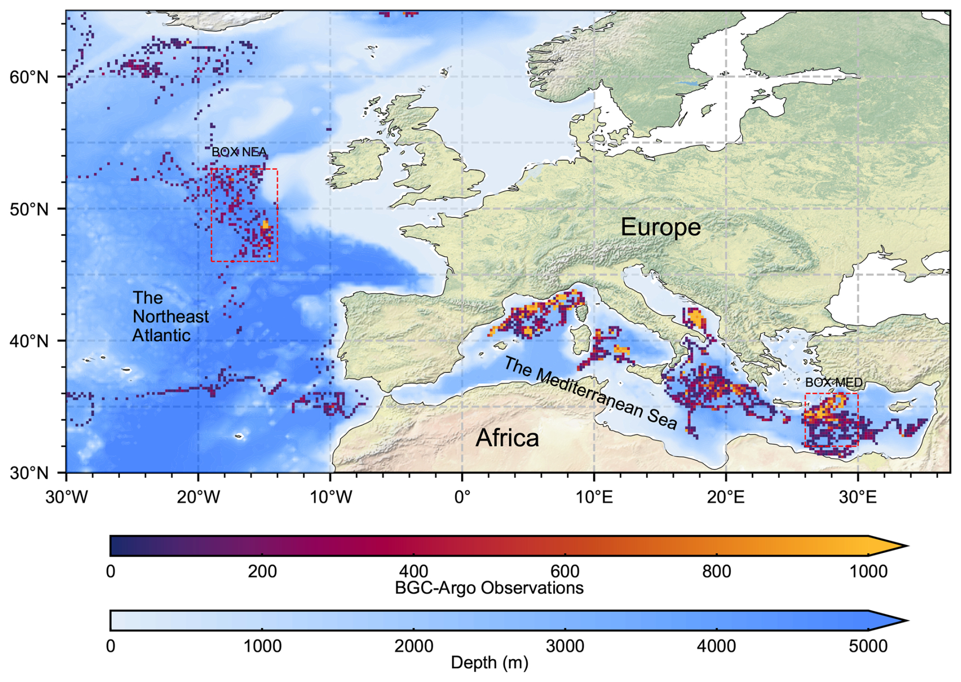
Figure 1 The pan-European domain, including the MED and the NEA. The study area is highlighted in blue, with shades of color indicating ocean depth. The warm-colored grid indicates the number of BGC-Argo observations. The two rectangular boxes are selected as typical data regions for pattern comparison.

Nutrients from the open ocean and river runoff create a general and rapid biogeochemical cycle in the NEA (Gattuso et al., 1998), in contrast to the MED, which is distinguished by its semi-enclosed and oligotrophy conditions. This study aims to develop a robust and generalizable modeling framework by exploring the relationships between multiple variables and validating its effectiveness in different marine regions.

2.2 Data

2.2.1 The in situ nitrate data

The in situ data of nitrate concentration used in this study were obtained through BGC-Argo (https://biogeochemical-argo.org/, last access: 13 June 2025, and https://www.ocean-ops.org, last access: 13 June 2025), a network of profiling floats equipped with sensors capable of monitoring six biogeochemical variables (Claustre et al., 2020). The time, longitude, latitude, and pressure representing the depth are also recorded during the observations. Nitrate concentration is measured using ultraviolet absorption spectroscopy (Johnson et al., 2024), with an average accuracy of ±0.5 µmol kg⁻¹ (Johnson et al., 2021, 2017; Mignot et al., 2019). In this study, a total of 477 870 data in the study area are used, with 409 011 collected from the MED and 68 859 from the NEA.

The GLODAPv2 database (https://doi.org/10.25921/1f4w-0t92, Lauvset et al., 2022b) provides a uniformly calibrated open-ocean data product with inorganic carbon and carbon-relevant variables (Lauvset et al., 2022a, 2021; Olsen et al., 2020). GLODAPv2 contains 15 cruises within the study area, which are utilized for independent validation of the model's predictive performance.

2.2.2 Simulated nitrate data

While the BGC-Argo network provides a significant amount of in situ data on nitrate concentration, its spatial coverage remains inadequate for the entirety of the ocean. Notably, BGC-Argo deployments are sparse in the NEA and coastal areas, where nitrate concentrations are higher and of greater environmental concern (Berglund et al., 2023; Moore et al., 2013). Conventional deep-learning algorithms typically only perform well when there is great similarity between test and training datasets. The lack of comprehensive in situ observations can introduce bias into the training dataset, adversely affecting the performance and generalization ability of the model. Hence, integrating BGC-Argo nitrate observations with broad simulated nitrate data becomes crucial.

Simulated nitrate data are obtained from CMEMS. The GLOBAL_MULTIYEAR_BGC_001_029 (https://doi.org/10.48670/moi-00019, Copernicus, 2024) product provides daily and monthly analyses of biogeochemical variables with a horizontal resolution of 0.25°×0.25° and features 75 vertical levels. These products are based on the Pelagic Interactions Scheme for Carbon and Ecosystem Studies (PISCES) biogeochemical model (Aumont et al., 2015), which is part of the Nucleus for European Modelling of the Ocean (NEMO) modeling platform (Madec, 2016). The model can simulate biogeochemical cycles across various oceanic provinces and has been employed successfully in various biogeochemical studies (Tian et al., 2022; Yang et al., 2024).

2.2.3 Matching sea surface environmental variable datasets

Sea surface environmental variables (SSEVs) matched to in situ nitrate data are used as input features for the model, as detailed in Table 1. The SSEV data all span the period from 2010 to 2023, matching the BGC-Argo data since 2012 and enabling the reconstruction of the 3D nitrate field since 2010.

Table 1 Details of the SSEV dataset.

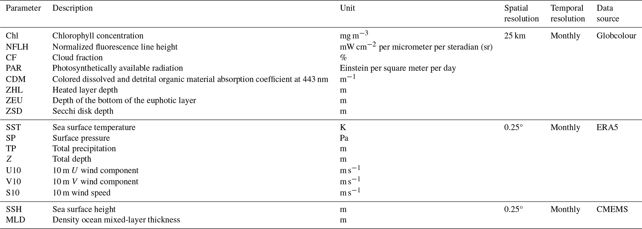
The satellite-derived ocean color data were obtained from the European Space Agency's Global Color Project (Lavender et al., 2009; Stéphane et al., 2010), with a spatial resolution of 25 km and a monthly temporal resolution (https://hermes.acri.fr, last access: 13 June 2025). The meteorological driver data were taken from the ERA5 dataset (Hersbach et al., 2020) (https://cds.climate.copernicus.eu, last access: 13 June 2025), with a spatial resolution of 0.25° and the temporal resolution of the monthly averaged reanalysis. ERA5 is the fifth-generation European Centre for Medium-Range Weather Forecasts (ECMWF) atmospheric reanalysis of the global climate. Reanalysis combines model data with observations in a globally complete and consistent dataset. CMEMS provides ocean-dynamics-related data, which have a spatial resolution of 0.25° and a monthly averaged temporal resolution.

2.3 Methods

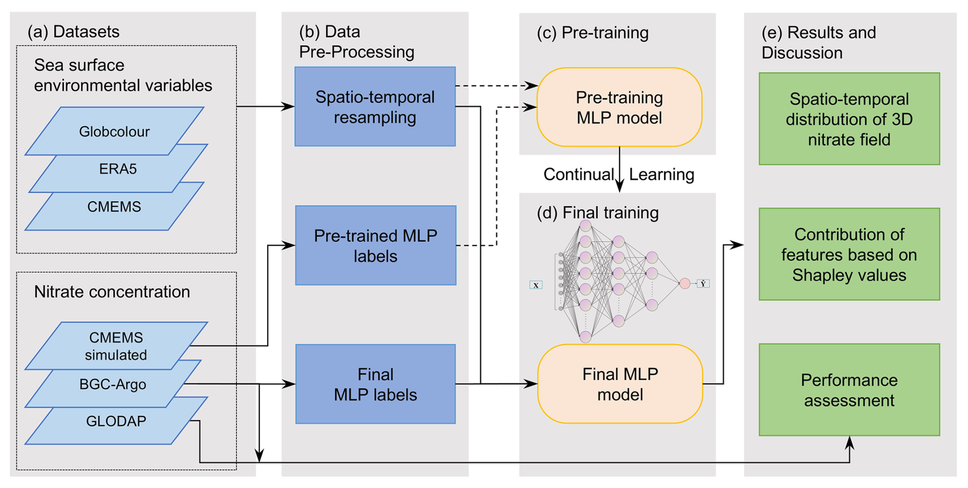
Figure 2 depicts the process of estimating nitrate and related research in this paper. The SSEVs and spatiotemporal coordinates undergo data preprocessing and resampling (Sect. 2.3.1) to serve as the feature set for the two-step training of the MLP model. The simulated and BGC-Argo nitrate concentrations provide the constructed MLP model (Sect. 2.3.2) with labels for two-stage continual-learning (Sect. 2.3.3) training. So far, the MLP has completed the modeling of the relationship between the surface environment and the internal ocean nitrate. After undergoing four kinds of 3D performance validations, the model reconstructed the 3D nitrate field by inputting iterated spatiotemporal coordinates and the corresponding SSEV datasets. The feature contributions and the potential mechanisms for estimation were evaluated based on the training datasets and the model (Sect. 2.3.5).

Figure 2 Workflow for nitrate estimation and research on reconstructed results.

2.3.1 Data preprocessing

The candidate input variables for estimating nitrate are depth, latitude, longitude, day of the year, and the SSEV data mentioned in Sect. 2.2.3. The time variables (day of the year) and geographical coordinates (latitude, longitude, and depth) are intended to explain the temporal and spatial variations of the studied parameters. The characteristics of biogeochemistry in the ocean properties are described by SSEVs such as SST and Chl (D'Ortenzio and Ribera d'Alcalà, 2009). Furthermore, variables such as sea surface height (SSH) provide insights into the ocean dynamics, which may contribute to obtaining more accurate vertical stratification.

All these predictor variables are utilized as input features after preprocessing. By standardizing and resampling, they were matched to nitrate concentration measurements, serving as features and labels to train the MLP (Fig. 2b). The potential uncertainty in the input features can be reduced significantly by implicitly incorporating them into the weights of the model when utilizing the same data products (Chen et al., 2019). The gridded SSEV data underwent limited linear interpolation along longitude, latitude, and time, refining localized missing values while filtering out extensive data gaps. Subsequently, the SSEV feature set was linearly interpolated and resampled to align with the spatiotemporal coordinates of nitrate data, ensuring that grid features with missing neighboring coordinates were excluded to prevent low-quality data from adversely affecting model training.

To utilize the annual period, the sampling dates are projected onto the circular coordinates as follows:

$$\begin{array}{}\text{(1)}& {\displaystyle }& {\displaystyle }\mathrm{Jday}\mathrm{1}=\cos (\mathrm{2}\mathit{\pi }\cdot (\mathrm{day}\mathrm{of}\mathrm{year}/\mathrm{365}\left)\right),\text{(2)}& {\displaystyle }& {\displaystyle }\mathrm{Jday}\mathrm{2}=\sin (\mathrm{2}\mathit{\pi }\cdot (\mathrm{day}\mathrm{of}\mathrm{year}/\mathrm{365}\left)\right).\end{array}$$

The other input features are then normalized by applying Z-score transformations as follows:

$$\begin{array}{}\text{(3)}& z\left(x_i\right)=\left(x_i-\mathit{\mu }\right)/\mathit{\sigma },\end{array}$$

where μ and i are the mean and standard deviation of each feature of the training set and x_i is the input value of feature i. Z-score transformation is a linear normalization technique commonly used in MLP development to align the inputs and intended outputs within comparable value ranges.

2.3.2 Multilayer perceptron

The study develops an MLP (Bishop, 1995) model, which is a type of feed-forward neural network that can be used for various types of input or output mappings (Hagan et al., 1997). MLPs can approximate any continuous and derivable function by means of an error backpropagation algorithm (Rumelhart et al., 1986). An MLP consists of interconnected neurons organized into input, hidden, and output layers. Each connection is assigned a weight w, and the output is generated by combining inputs and weights using an activation function after adding the neuron's bias b_j. The weights are iteratively updated during the training epochs to minimize the loss function, which reduces the quadratic error between the MLP outputs and labels. This iterative process continues until a minimum is reached using the approach of error backpropagation.

The structure of the MLP is determined by a series of experiments with multiple hidden layers, and it utilizes the LeakyRelu activation function. The optimal network is determined through multiple trials, where the structure with the least amount of error in the test dataset and the fewest neurons is selected. The final network was configured as (22-128-64-16-1), comprising one input layer with 22 inputs, three hidden layers with 128, 64, and 16 nodes, and one output layer with the nitrate concentration as the output value.

2.3.3 Continual learning

The generalization capability of deep-learning models, including MLPs, is highly dependent on the representativeness of the training data. Insufficient or imbalanced training data can exacerbate generalization errors and increase the risk of model overfitting. In the domain of water resource research, challenges associated with the collection of in situ data have highlighted the effectiveness of transfer learning (TL) techniques (Cao et al., 2020; Harkort and Duan, 2023; Miao et al., 2023; Syariz et al., 2020; Zhu et al., 2017). Nevertheless, most TL applications are based on fine-tuning (Ma et al., 2024), which limits their capacity to integrate knowledge from multiple datasets in a more comprehensive manner (Zhou and Zhang, 2023). To overcome this limitation, we developed the continual-learning (CL) strategy to improve the training process of BGC-Argo. CL enables the model to assimilate new knowledge continually while retaining previously acquired information, thereby enhancing the robustness and adaptability of the model.

In practice, the simulated nitrate data are initially employed for pre-training, after which the derived network weights are transferred to the subsequent training phase supervised by BGC-Argo observations. Ideally, this sequential process enables the model to capture the general distribution patterns and underlying variation mechanisms present in the simulated nitrate data and subsequently to refine its estimations to achieve higher accuracy using BGC-Argo measurements. However, when the model undergoes incremental training through gradient-based updates, it may experience catastrophic interference or forgetting, leading to the degradation of previously acquired knowledge (Kirkpatrick et al., 2017). To address this issue, elastic weight consolidation (EWC), a regularization-based continual-learning algorithm, is applied to constrain weight updates by assigning greater importance to critical network parameters (Kirkpatrick et al., 2017).

Figure 3 (Kirkpatrick et al., 2017) illustrates the effect of training strategies on the two-stage training task and how EWC ensures the retention of knowledge from Task A during the learning of Task B. Sets A and B represent the solution spaces for the two training tasks, specifically the simulated nitrate and BGC-Argo training. After completing Task A, the parameters are labeled ${\mathit{\theta }}_{\mathrm{A}}^{*}$, and the three trajectory lines depict different training processes under varying loss function constraints. Constraining each weight equally (green arrow) imposes excessively rigid restrictions, allowing Task A to be retained only at the cost of failing to learn Task B. Conversely, applying gradient steps based solely on Task B (blue arrow) effectively minimizes the loss for Task B but compromises the knowledge acquired from Task A. Although BGC-Argo measurements are accurate, they are limited in their spatiotemporal coverage for nitrate reconstruction studies, which is insufficient for a comprehensive global characterization of nitrate distributions. Consequently, the center of Set B represents the optimal solution for model weights in the BGC-Argo training set, but this is overfitted and suboptimal for broader global reconstruction. In contrast, the EWC trajectory (red line) finds an optimal balance for Task B while calculating the importance of weights for Task A, thus ensuring minimal loss in Task A's performance. Robust weights should lie between Sets A and B, balancing the broad and generalizable knowledge from simulated nitrate with the precise measurements from BGC-Argo. This process can be understood as guiding the model to retain the broad knowledge to enhance the generalization ability of Task B or as calibrating the simulated nitrate with the precision of BGC-Argo. Given that simulated nitrate provides concentration data across the entire ocean, especially in regions not yet observed by BGC-Argo, this strategy is crucial for enhancing the generalization capability and robustness of the MLP model.

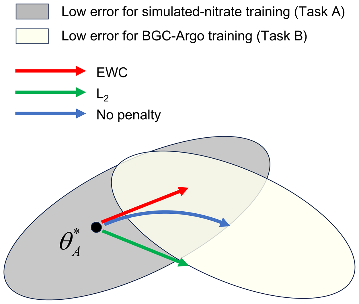
Figure 3 Schematic illustration of how training strategies influence study trajectories in a two-stage task (Kirkpatrick et al., 2017).

EWC relies on the Fisher information matrix (FIM) to estimate the importance of each model parameter concerning previous tasks (Fisher and Russell, 1997). The FIM quantifies the amount of information that an observable random variable carries about an unknown parameter, reflecting how sensitive the likelihood function is to changes in the parameters. The FIM F is defined as

$$\begin{array}{}\text{(4)}& F={\mathbb{E}}_{x,y\sim p_{\mathrm{data}}(x,y)}\left[{\mathrm{\nabla }}_{\mathit{\theta }}\log p\left(y\right|x;\mathit{\theta }\left){\mathrm{\nabla }}_{\mathit{\theta }}\log p\right(y|x;\mathit{\theta }{)}^{\top }\right],\end{array}$$

where $p\left(y\right|x;\mathit{\theta })$ is the likelihood of the target y of the given data x and model parameter θ, and ${\mathrm{\nabla }}_{\mathit{\theta }}\log p\left(y\right|x;\mathit{\theta })$ is the gradient of the log-likelihood with respect to the parameters.

In practical applications, computing the full FIM is computationally expensive, particularly for large neural networks. To simplify the computation, it is often assumed that the FIM is diagonal, effectively ignoring dependencies between parameters. In MLPs, the diagonal elements of the FIM can be approximated as follows:

$$\begin{array}{}\text{(5)}& F_i\approx {\mathbb{E}}_{x,y\sim p_{\mathrm{date}}(x,y)}\left[{\left({\displaystyle \frac{\partial \log p\left(y\right|x,\mathit{\theta })}{\partial {\mathit{\theta }}_i}}\right)}^{\mathrm{2}}\right].\end{array}$$

Since the true distribution of the data is unavailable, the training data are typically used for estimation:

$$\begin{array}{}\text{(6)}& F_i\approx {\displaystyle \frac{\mathrm{1}}{N}}\sum _{n=\mathrm{1}}^N{\left({\displaystyle \frac{\partial \log p\left(y_n|x_n,\mathit{\theta }\right)}{\partial {\mathit{\theta }}_i}}\right)}^{\mathrm{2}},\end{array}$$

where N is the number of training samples, (x_n y_n) are the data samples, and θ_i is the ith parameter of the model.

In regression tasks using MLPs, we model the output y as

$$\begin{array}{}\text{(7)}& y=f(x;\mathit{\theta })+\mathit{ϵ},\mathit{ϵ}\sim \mathcal{N}\left(\mathrm{0},{\mathit{\sigma }}^{\mathrm{2}}\right).\end{array}$$

Assuming Gaussian noise with a constant variance σ², the diagonal elements of the FIM can be approximated based on the gradients of the model's output with respect to its parameters. Specifically, we compute F_i as

$$\begin{array}{}\text{(8)}& F_i\approx {\displaystyle \frac{\mathrm{1}}{N}}\sum _{n=\mathrm{1}}^N{\left({\displaystyle \frac{\partial f\left(x_n;\mathit{\theta }\right)}{\partial {\mathit{\theta }}_i}}\right)}^{\mathrm{2}},\end{array}$$

where x_n is the nth input sample and $\frac{\partial f(x_n;\mathit{\theta })}{\partial {\mathit{\theta }}_i}$ is the partial derivative of the model output with respect to parameter θ_i. This approximation allows efficient computation of F_i during training.

In the Bayesian framework, the goal is to find the parameter θ that maximizes the posterior probability given both the previous task data D_A and the new task data D_B:

$$\begin{array}{}\text{(9)}& p\left(\mathit{\theta }|D_{\mathrm{A}},D_{\mathrm{B}}\right)\propto p\left(D_{\mathrm{B}}|\mathit{\theta }\right)p\left(\mathit{\theta }|D_{\mathrm{A}}\right).\end{array}$$

Since directly computing p(θ|D_A) is intractable, we approximate it using a Gaussian distribution centered at the previous optimal parameters ${\mathit{\theta }}_{\mathrm{A}}^{*}$, with the precision given by the FIM (MacKay, 1992):

$$\begin{array}{}\text{(10)}& p\left(\mathit{\theta }|D_{\mathrm{A}}\right)\approx \mathcal{N}\left({\mathit{\theta }}_{\mathrm{A}}^{*},F^{-\mathrm{1}}\right).\end{array}$$

Taking the negative logarithm of the posterior and ignoring constants independent of θ, we obtain the total loss function:

$$\begin{array}{}\text{(11)}& L_{\mathrm{EWC}}\left(\mathit{\theta }\right)=L_{\mathrm{B}}\left(\mathit{\theta }\right)+{\displaystyle \frac{\mathit{\lambda }}{\mathrm{2}}}\sum _i{F}_i{\left({\mathit{\theta }}_i-{\mathit{\theta }}_{\mathrm{A},i}^{*}\right)}^{\mathrm{2}},\end{array}$$

where L_B(θ) is the loss for the new task only, i is each parameter, F_i is the FIM of the previous task, ${\mathit{\theta }}_{\mathrm{A}}^{*}$ is the optimal parameter value after training on the previous task, and λ is a hyperparameter controlling the tradeoff between performance of the new task and retention of the previous task's knowledge.

2.3.4 Model validation

Nitrate concentrations derived from the identical vertical observations by BGC-Argo exhibit a strong correlation and a gradual variation with increasing depth. Conventional methods that divide the entire dataset proportionally can result in highly similar data appearing in both the training and test sets, thereby leading to an exaggerated model performance (Salazar et al., 2022). Hence, it is imperative to partition the BGC-Argo dataset based on the observation period, with each period referred to as a profile (Sammartino et al., 2020; Sauzède et al., 2017). This division method ensures the identical distribution and independence of the training and test sets. Furthermore, the spatial generalization capabilities of the model can be assessed further by partitioning the dataset based on devices.

A five-fold cross-validation approach is employed to evaluate the model performance using independent test data; this is widely used in machine learning. The BGC-Argo dataset was evenly divided into five subsets based on profiles or sites. In five distinct cycles, each subset (approximately 20 % of the total dataset) served as the test set for one fold, with the remaining four subsets used to train the MLP model. Upon completion of the five folds, all BGC-Argo data were used for one test and four training sessions. This process mitigates the influence of data partitioning bias on performance validation, ensuring maximal data utilization and providing a more robust evaluation of the model's generalization capability. In the test set, the MLP performance was evaluated by comparing the estimated values with in situ nitrate values, using statistical metrics such as the determination coefficient (R²), mean bias error (MBE), mean square error (MSE), root mean square error (RMSE), mean absolute error (MAE), and median absolute error (MedAE).

2.3.5 Evaluating the contribution of inputs

Another major limitation of MLPs and deep-learning networks is the lack of interpretability, which makes it challenging to evaluate the estimation processes and mechanisms. However, it is essential to assess the validity of environmental parameters for estimating nitrate concentration, especially since their influence and interactions are not fully elucidated.

Shapley values (Shapley, 1988) form a method in coalition game theory that effectively describes how benefits are fairly distributed among contributions by the difference between the predicted and average predicted values in each case. The Shapley value of a feature is its weighted and summed contribution to the output over all possible feature combinations:

$$\begin{array}{}\text{(12)}& \begin{array}{rl}{\mathit{\varphi }}_j\left(\mathrm{val}\right)=& \sum _{S\subseteq \mathit{\{}\mathrm{1},\mathrm{\dots },p}\mathit{\}}\backslash \mathit{\{}j\mathit{\}}{\displaystyle \frac{\left|S\right|\mathrm{!}(p-\left|S\right|-\mathrm{1})\mathrm{!}}{p\mathrm{!}}}\\ & \left(\mathrm{val}\right(S\cup \mathit{\left\{}j\mathit{\right\}})-\mathrm{val}\mathit{\{}S\mathit{\left\}}\right),\end{array}\end{array}$$

where ϕ_j is the contribution of the jth feature to the results. S is a subset of the model's features, and p is the total number of features. val(S) is the prediction for feature values in S that are marginalized over features not included in S.

Shapley additive explanations (SHAP) (Lundberg and Lee, 2017) form a method for explaining individual estimation results based on Shapley values, which have been applied successfully to evaluate predictors using machine learning algorithms in environmental research (Hu et al., 2023). The purpose of SHAP is to compute the contribution of each feature to the result to explain an instance. Shapley values are depicted as a linear additive feature attribution approach. SHAP specifies the explanation as

$$\begin{array}{}\text{(13)}& g\left(x^{\prime }\right)={\mathit{\varphi }}_{\mathrm{0}}+\sum _{j=\mathrm{1}}^M{\mathit{\varphi }}_j,\end{array}$$

where g is the model to be explained, M is the size of the feature space, and ϕ_j∈R is the feature contribution for feature j, which is the same as the Shapley values of j.

We can calculate SHAP to quantify the contribution of each feature to the prediction results of a black-box model in different samples. The feature tends to increase the output result when SHAP is positive. Conversely, the feature tends to decrease the output result when SHAP is negative. The absolute SHAP value (ASV) indicates the degree to which the feature affects the output. To observe the overall significance, the mean of the ASV for each feature in the data is therefore defined as

$$\begin{array}{}\text{(14)}& I_j={\displaystyle \frac{\mathrm{1}}{n}}\sum _{i=\mathrm{1}}^n\left|{\mathit{\varphi }}_j^{\left(i\right)}\right|,\end{array}$$

where i represents the data samples and j represents the features.

3 Results and discussion

3.1 Model performance

In the five-fold profile-based cross-validation, all of the data are used once in the test set. As illustrated in Fig. 4, the model performance is evaluated by comparing estimated values with BGC-Argo observations. The model demonstrates high accuracy in estimating nitrate concentration, with estimated values generally aligning along the 1:1 line. Importantly, to ensure a comprehensive dataset and to enhance the stability of the reconstruction process, we retained all of the measured labels, including negative values. Furthermore, a Softplus activation function was applied to the model's output layer to guarantee non-negative predictions, albeit at the expense of some degradation in statistical performance metrics. Considering the significant differences between the two regions of the study area, Fig. 4b and c show the test results for the MED and NEA. Compared to the NEA, the MED exhibits a smaller range of nitrate variations and stronger estimation performance. The MED records account for 86 % of the total dataset, whereas the NEA contributes only 14 %. This data imbalance likely contributes to the more consistent performance in the MED compared to the NEA.

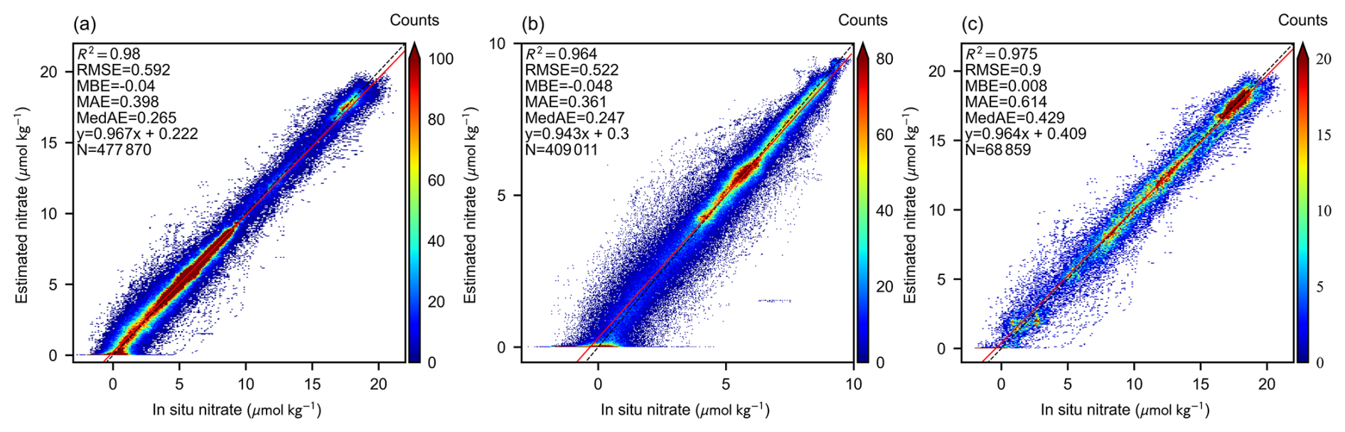
Figure 4 Estimation performance on the test set validated by BGC-Argo measurements (a). The test set results are further divided into the MED (b) and NEA (c) regions. The red line indicates the fitted trend of the data, while the black dashed line denotes the 1:1 parity line.

While the model has shown satisfactory overall performance, it is critical that the accuracy remains consistently desirable in the vertical dimension. Only then can the model fulfill its intended purpose of estimating and reconstructing the entire 3D ocean nitrate field. Figure 5 illustrates the vertical distribution of the primary statistical metrics and their comparison with simulated nitrate. The model maintains robust performance in the vertical dimension, with no significant fluctuations in RMSE and MBE, which is vital for accurately estimating nitrate profiles. The model exhibits slightly superior performance in the MED compared to the NEA at most depths. The RMSE in both the MED and NEA is higher between 0 and 150 m, with a notable peak at 60 m depth, reaching about 0.8 and 1.4 µmol kg⁻¹, respectively. Furthermore, the RMSE of the MED remains at a low level and slowly decreases as depth increases. In contrast, the RMSE of the NEA varies drastically, accompanied by a larger overall error, particularly in the 400–700 m depth range. As shown in Fig. 5b, MBE values are negative for most depth ranges in the NEA, suggesting a slight overall underestimation of nitrate concentrations, while a slight overestimation occurs in the upper-ocean layers of both subregions.

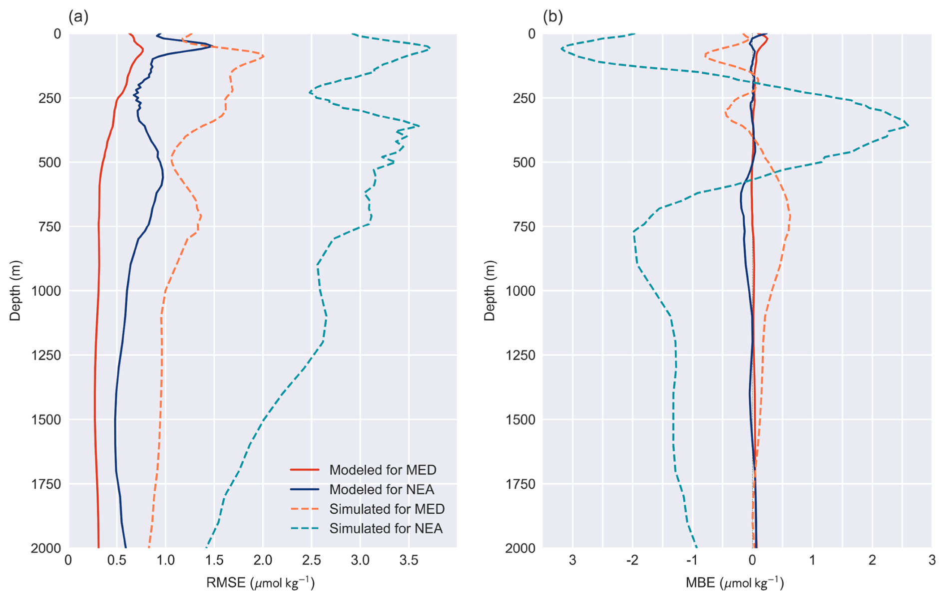
Figure 5 Vertical profiles of the RMSE (a) and MBE (b) for modeled and simulated nitrate compared to BGC-Argo measurements.

The model excels in the deep ocean layers beyond 800 m depth, where nitrates are characterized by low variability and minimal feedback from the sea surface environment. Nonetheless, through the use of temporal and spatial coordinates and a dual training process, the model accurately estimates nitrate concentrations. The model's relatively weak performance is observed at the upper 100 m depths, which could be attributed to the sensitivity of the surface layer to external nitrate inputs (Altieri et al., 2021), thus leading to deviations from the model-fitted relationship between nitrate and SSEVs. Furthermore, the ocean at these depths is usually influenced by both the euphotic layer and mixed layers, where complex interactions between ecosystem and ocean dynamics occur, such as water transport, plankton consumption, and decomposition. Hence, predicting parameters at this depth has usually presented the biggest challenge in vertical dimension estimation (Sammartino et al., 2020).

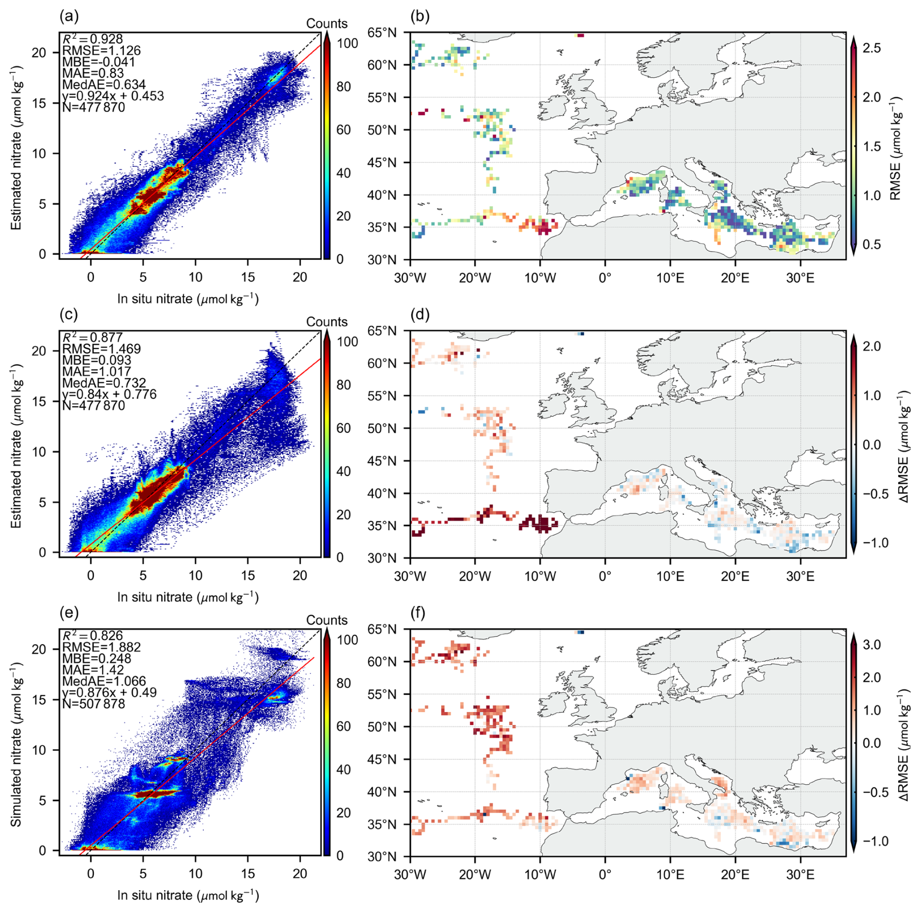
Figure 6 Illustration of model performance and spatial generalization in site-based cross-validation (a) and spatial error distributions (b), compared with the case without CL (c, d) and the case of simulated nitrate itself (e, f). The subplots show (a) the test performance with CL, (b) the spatial distribution of model accuracy, (c) the test performance without CL, (d) the distribution of RMSE increases (non-CL relative to CL), (e) the validation performance of simulated nitrate concentrations, and (f) the spatial distribution of RMSE increases (simulated nitrate relative to models with CL).

In contrast, simulated nitrate exhibits instability in describing the vertical distribution of nitrate concentration. Firstly, simulated nitrate produces significant errors at the ocean surface, possibly due to the limitations of biogeochemical models in simulating complex boundary interactions. However, the estimation error here has been significantly ameliorated by the MLP owing to the strong correlation between SSEVs and SSN. Secondly, the characterization of nitrate vertical changes by simulated nitrate is not precise enough. The vertical inaccuracy may result in disparities in the characterization of the changes, thus placing a limitation on small-scale biogeochemical research. An evident instance can be observed in the mesopelagic zone (MZ), ranging from 200 to 1000 m in the NEA. Simulated nitrate faced challenges in accurately describing the vertical rate of nitrate variations in this range, resulting in a notable overestimation of nitrate concentrations (Fig. 5b). This is also reflected in the distinct step-like pattern observed at nitrate concentrations of 10–15 µmol kg⁻¹ (Fig. 6a) and the overestimation in the vertical pattern (Fig. 8e). Furthermore, the MLP and simulated nitrate present similarities in the vertical profiles of the RMSE, while the MLP consistently outperforms simulated nitrate. This also demonstrates that the MLP has improved performance from incorporating prior knowledge from simulated nitrate through CL.

3.2 Spatial generalization ability and enhancement of continual learning

Due to the limited monitoring range of BGC-Argo, the spatial generalization ability of the model is crucial for accurately reconstructing the complete nitrate concentration field. Therefore, this section adopts a more rigorous validation procedure by partitioning the BGC-Argo dataset according to device sites and performing the five-fold cross-validation as outlined in Sect. 2.3.4. Under these circumstances, the spatial disparity between the training and test sets grows significantly, aiding in the assessment of the model's predictive performance across unknown marine regions and amplifying the comparative impact of CL on spatial generalization.

Figure 6e illustrates the accuracy of simulated nitrate concentrations by interpolating gridded simulated nitrate data across longitude, latitude, depth, and time to match the spatiotemporal coordinates of BGC-Argo observations, thereby approximating and validating the simulated values. The results indicate that simulated nitrate tends to form stepwise clusters due to its inertia and lack of variability in representing localized nitrate fluctuations (Fig. 8), leading to similar y values within subsets that should correspond to x-direction gradients. Nevertheless, the overall agreement between the two datasets remains strong. The simulated nitrate achieves an acceptable accuracy (R²=0.826, RMSE = 1.882 µmol kg⁻¹), making it a valuable prior dataset. This compatibility is crucial, and given that simulated nitrate can provide data of comparable accuracy across the entire ocean, its shows great potential as a complement to BGC-Argo data. Simulated nitrate aids in understanding the large-scale distribution of nitrate, offering extensive insights that serve as a beneficial foundation for enhancing fitting relationships during subsequent CL training phases.

Figure 6a illustrates the spatial generalization test performance of the model, demonstrating that CL leads to enhanced test performance, as marked by an increase in R² of 0.051 and a decrease in RMSE of 0.343 µmol kg⁻¹, compared to the non-CL results shown in Fig. 6c. Specifically, the MLP model without CL significantly underestimates high nitrate concentration samples, primarily due to its limited generalization ability in unfamiliar regions of the NEA during site-specific cross-validation. The introduction of CL effectively mitigates this limitation, allowing the model to maintain stable generalized estimates, even for high nitrate concentration samples. Furthermore, the majority of the samples exhibit a more consistent fit to the 1:1 line, significantly reducing the episodic uncertainty associated with simulated nitrate and the generalization error of the non-CL MLP model. Notably, coupling with CL retains the influence of prior knowledge from simulated nitrate, resulting in localized variability differences. For instance, the densely packed high-concentration samples in warm colors transitioned from symmetric fitting (Fig. 6c) to step-like clustering (Fig. 6a) while achieving a closer fit and overall improved performance. The extent of this transformation is influenced by the EWC parameter λ.

Figure 6b presents the horizontal distribution of the RMSE. The predictions exhibit the highest accuracy in the central MED, while larger RMSE values are observed in the NEA and peripheral regions of the MED. The substantial variability in nitrate concentrations in the NEA is largely attributable to the active exchange of eutrophic seawater. Furthermore, the sparse distribution of BGC-Argo measurements in the NEA results in significant deviations from the training data, posing substantial challenges to accurate cross-validation in this region. Overall, high error rates are frequently observed in coastal locations, particularly in the western Strait of Gibraltar and the southern parts of the MED. These areas are more susceptible to anthropogenic influences and complex land–sea interactions, which complicate prediction efforts. Additionally, the shallower topography of these regions contributes to increased errors in the vertical water column, particularly in the error-prone ocean surface layer (Fig. 5a).

Notably, regional disparities introduced by CL are evident in Fig. 6d. When the peripheral regions are used as test sets, the discrepancies between training and test data distributions become more pronounced. This sparsity of BGC-Argo data poses a considerable challenge for model estimation in regions lacking sufficient global training on similar datasets, leading to reduced performance metrics. However, CL significantly enhances the model's estimation capabilities in sparsely observed regions, particularly in areas with high RMSE values near the boundaries of BGC-Argo coverage. This suggests that CL helps reduce model instability when generalizing to unfamiliar regions by incorporating prior knowledge from simulated nitrate. For instance, in the western Strait of Gibraltar, complex environmental interactions and similarities in spatial coordinates to the MED present significant estimation challenges. Nevertheless, the model demonstrates substantial improvements in both accuracy and generalization stability compared to the MLP without CL. Moreover, the model achieves more accurate estimates by fitting BGC-Argo data, showing a comprehensive improvement over simulated nitrate (Fig. 6f), which is critical for reconstructing the 3D nitrate field. Interestingly, in data-dense regions such as parts of the Mediterranean, the incorporation of CL results in a slight increase in the RMSE. This phenomenon occurs because, in well-sampled regions, prior knowledge may interfere with the MLP's fitting process. However, the influence of this prior knowledge can be optimized by regionally adjusting the EWC parameter λ. Currently, this parameter is selected to achieve an overall optimal performance.

In conclusion, it is reasonable to infer that CL enhances the overall model performance and generalization capability in regions not covered by BGC-Argo by incorporating relevant knowledge and patterns from simulated nitrate. This process is influenced by data distribution and weighting parameters.

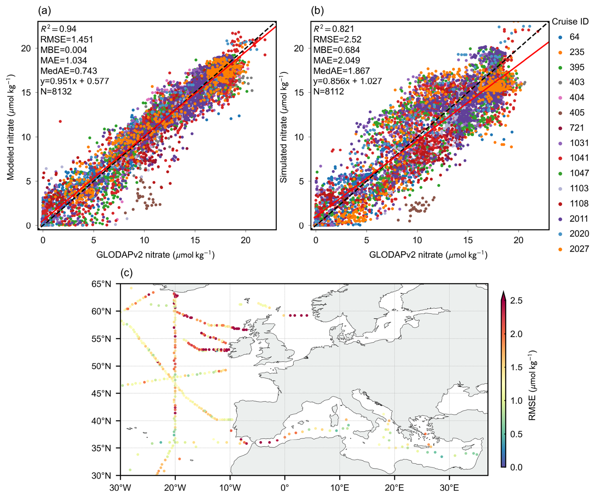
Figure 7 Accuracy comparison between MLP-estimated nitrate (a) and simulated nitrate (b), using GLODAPv2 measurements for validation, with the colors denoting individual cruises. The subplots show (a) validation of MLP-estimated nitrate, (b) validation of simulated nitrate, and (c) the spatial RMSE distribution of MLP-estimated nitrate, where the errors are derived from the average vertical measurement error at each cruise sampling location.

3.3 Independent validation with GLODAPv2

To further ensure a more stable assessment of the model's generalization ability in data-sparse regions while avoiding potential autocorrelation within the BGC-Argo dataset, the GLODAPv2 database was employed for independent validation, which was not part of the training. Fifteen cruises measuring nitrate concentrations at depths ranging from 0 to 2000 m in the study area were selected, and their measurements were compared against model estimates and simulated nitrate. Figure 7c illustrates that a significant portion of the GLODAPv2 data is located in the NEA, thereby allowing for an effective assessment of the model's performance in undersampled regions. The results indicate a strong correlation with the GLODAPv2 nitrate concentrations, as evidenced by an R² value of 0.94 (Fig. 7a).

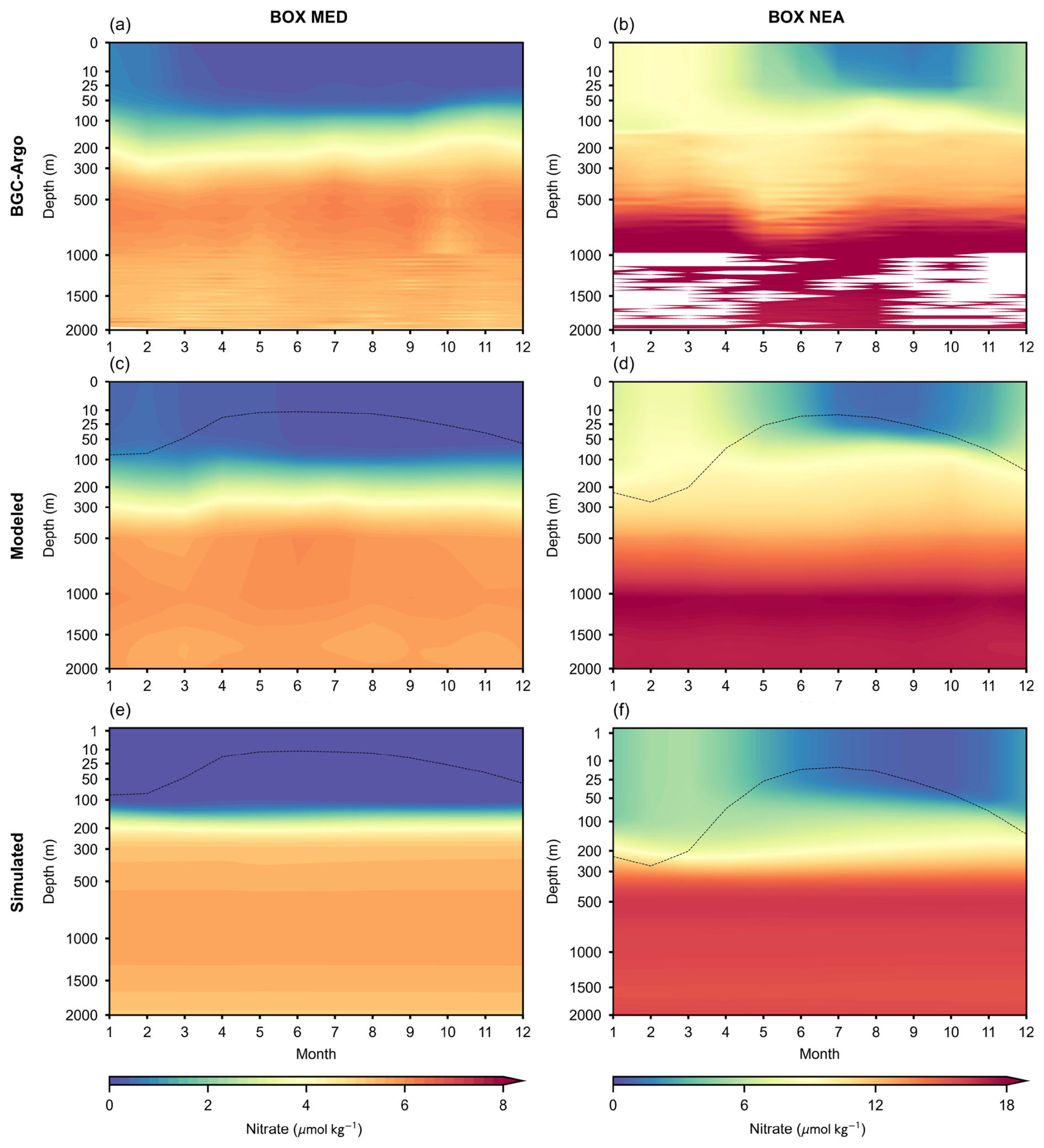
Figure 8 Comparison of monthly vertical patterns of nitrate in the designated region between BGC-Argo, the MLP model, and the simulated climatology. Panels (a), (c), and (e) correspond to the box MED, while panels (b), (d), and (f) correspond to the box NEA. The black dashed lines represent the average MLD from the CMEMS dataset.

Figure 7c also depicts the regional distribution of errors, revealing that model performance varies significantly across different regions. The lowest errors are observed in the western MED and the southern NEA, whereas larger errors are concentrated in areas with sparse BGC-Argo observations. This distribution pattern and its underlying causes align with the spatial performance in site-based cross-validation, as shown in Fig. 5b. Factors such as enhanced water exchange dynamics (Berglund et al., 2023), intricate land–sea interactions, and shallow topography contribute additional complexities. Moreover, several expeditions north of 50° N took place in 2010–2012 and 2015, while most BGC-Argo observations in the same region were made after 2020. The pronounced variability of nitrate concentrations in the NEA, coupled with limited observations and temporal discrepancies, diminishes the data representativeness, leading to an increased RMSE. Overall, the error margins are deemed acceptable and still outperform the validation accuracy of the simulated nitrate (Fig. 7b).

3.4 Validation of the 3D nitrate pattern

To thoroughly examine and contrast the seasonal vertical patterns of BGC-Argo, modeled, and simulated nitrate, two representative regions depicted in Fig. 1 were selected to facilitate a comprehensive evaluation of the model's efficacy. The box NEA, located at 14–19° W and 46–53° N, and the box MED, located at 26–30° E and 32–36° N, were chosen due to their frequent BGC-Argo sampling, which ensures great consistency between measured data and observed vertical patterns. The vertical distribution of nitrate is depicted in Fig. 8 for these two regions, where the MLP model, simulated nitrate, and BGC-Argo observations are juxtaposed for comparison.

The reconstructed vertical nitrate profiles derived from the MLP model demonstrate greater consistency and robustness compared to the BGC-Argo data, whereas the profiles from simulated nitrate still exhibit significant discrepancies in capturing seasonal variations. The MLP model has shown a remarkable ability to capture medium-scale features, such as the seasonal increase during winter and decrease during summer, aligning well with the BGC-Argo data and effectively depicting seasonal variations in the upper ocean. Furthermore, the MLP model is consistent with BGC-Argo in representing depth-dependent variability within the MZ while bridging gaps left by the intermittent nature of BGC-Argo measurements. In contrast, simulated nitrate tends to underestimate concentrations in the upper ocean (Fig. 5b) and shows relatively sluggish seasonal variations, including the absence of a pronounced increase during winter in the box NEA and insufficient representation of seasonal changes in the upper layers of the box MED.

As discussed previously, the model's estimation results demonstrate satisfactory accuracy and strong performance in the test dataset. Additionally, the model's predictions have been analyzed comprehensively across the vertical, horizontal, and temporal dimensions, all indicating high performance. To ensure robust generalization across diverse oceanic environments, the joint model was employed to estimate nitrate concentrations in both the MED and NEA, despite facing specific challenges. Given the complexity of the marine environment and the fact that the NEA represents only 14 % of the dataset, a higher error rate in this region is acceptable. Despite increased errors in some challenging cases, the model generally proves to be reliable for reconstructing the 3D nitrate concentration field.

3.5 Spatial and temporal distribution of the reconstructed nitrate field

The reconstruction of the 3D nitrate field from 2010 to 2023 was done using the MLP model combined with the SSEV for the corresponding period. The reconstructed field features a monthly temporal resolution, a horizontal spatial resolution of 0.25°, and 63 depth levels, with vertical intervals ranging from 5 to 50 m. Figure 9 illustrates the spatial distributions of the reconstructed nitrate at various depths across the pan-European region, with representative profiles selected at depths of 0, 50, 100, 150, and 500 m.

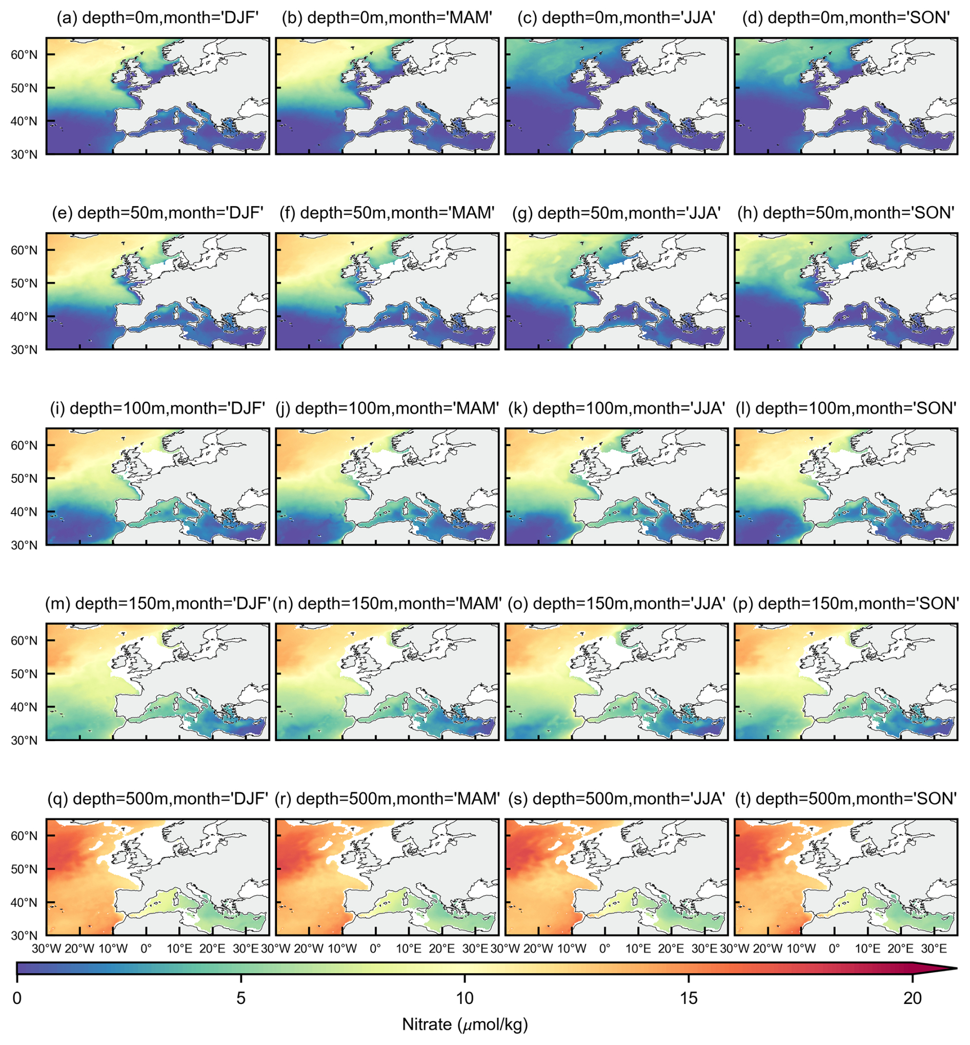
Figure 9 Spatial distribution of the reconstructed nitrate field, with the columns representing the four seasons and the rows representing the five depth slices.

The reconstructed nitrate field reveals substantial spatial variability, with a clear increasing trend in nitrate concentrations with depth. The MED was identified as an oligotrophic region and generally exhibits nitrate concentrations below 5 µmol kg⁻¹ at depths between 0 and 150 m. Unlike the NEA, the MED nitrate concentrations are less influenced by seasonal dynamics, primarily due to the region's enclosed nature and restricted seawater exchange. The oligotrophic characteristics of the MED intensify from west to east, with more pronounced differences evident in the deeper ocean layers (Pujo-Pay et al., 2011; Ribera d'Alcalà et al., 2003). In contrast, the NEA is characterized by higher nitrate concentrations and pronounced seasonal variability, which is largely driven by the influx of nutrient-rich water masses from the open ocean (Berglund et al., 2023). The highest nitrate concentrations are found in the NEA seawaters, which form a typical eutrophic region. The spatial pattern of the reconstructed results overall aligns well with that of the simulated nitrate dataset (Fig. S1 in the Supplement), including extensive regions not covered by BGC-Argo, such as the coastal waters of the UK and Norway. Meanwhile, discrepancies are observed in certain small-scale 3D structures between the reconstruction and the simulated nitrate field. These differences have the potential to provide valuable data foundations and insights for further ecological research.

Figure 10 presents the time–depth profiles of nitrate concentration as a function of the month in both the MED and NEA, allowing for a more detailed examination of their temporal patterns. The seasonal variability of nitrate in the MED is relatively subtle. During winter, upwelling of nutrient-rich cold water elevates nitrate concentrations in the upper ocean, with a marked increase observed from October to February of the following year. After reaching this peak, nitrate levels decline due to phytoplankton uptake during spring, followed by a secondary rise in fall as phytoplankton biomass decays (Severin et al., 2017). Conversely, the NEA exhibits a pronounced temporal pattern in nitrate concentration that is primarily governed by ocean dynamics. In the mixed layer, from the surface to a depth of approximately 100 m, nitrate levels increase from October to March and subsequently decrease from April to August. The temporal pattern in the NEA resembles the winter increase observed in the MED but lacks a distinct secondary peak, instead showing a more sustained high-nutrient period.

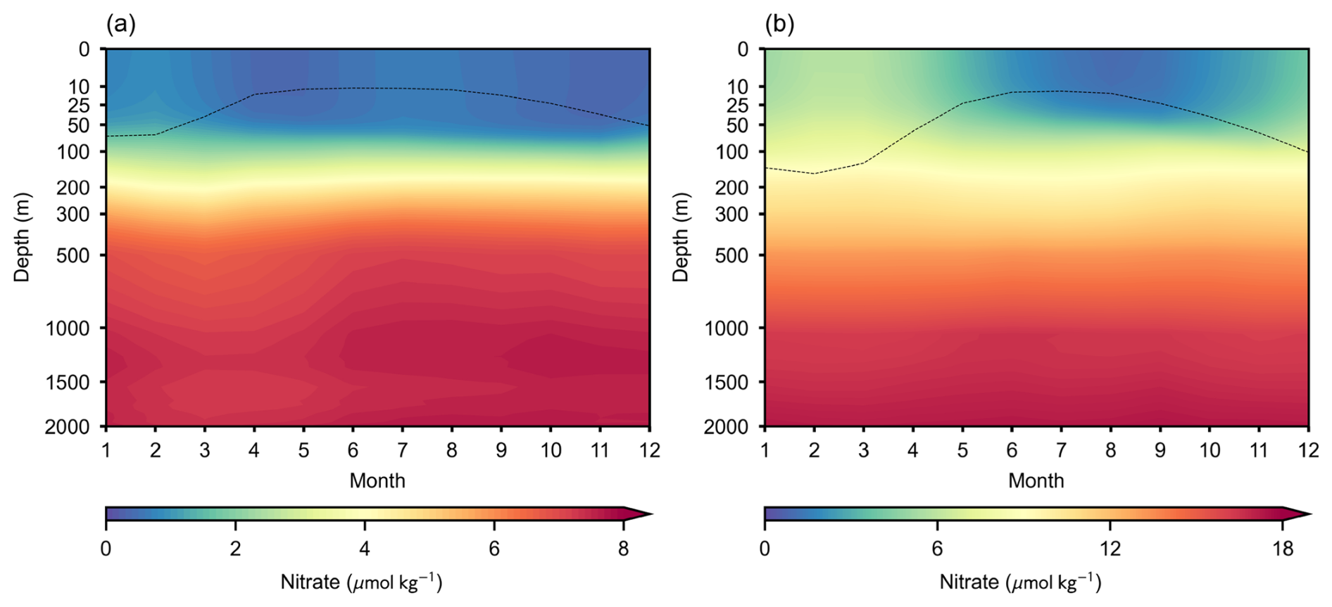
Figure 10 Monthly distribution profiles of nitrate concentrations in the MED (a) and NEA (b). The black dashed lines represent the average MLD from the CMEMS dataset.

Figure 11 illustrates the interannual anomalies of nitrate concentrations across the study area, derived by subtracting the annual mean nitrate value for each year from the monthly nitrate concentrations. In most instances, nitrate anomalies exhibit consistency throughout the vertical profile, with this uniformity being more pronounced in the MED. Additionally, episodic discontinuities are often detected at depths around 100 and ≈500 m, corresponding to the mixing layer and certain pycnoclines. In the NEA, where seawater exchange is more dynamic, discontinuities in nitrate concentration are more prevalent. Compared with existing data sources, although BGC-Argo and simulated nitrate represent some of the most advanced nitrate data available from current observational and numerical models, they still face significant challenges in depicting interannual trends (Fig. S2). Due to the varying geographical locations of BGC-Argo observations over time, regional differences in nutrient levels introduce considerable interference and fluctuations into the calculation of interannual trends. Consequently, the trends presented by BGC-Argo appear to be more radical and may even be reversed if the sampling locations encompass both high- and low-nutrient regions. As for CMEMS nitrate, its response to mesoscale nitrate variations is relatively sluggish, leading to an overly homogeneous trend that is likely more conservative than the actual scenario. Nevertheless, its overall trend can serve as a reference for multiyear scale variations, such as the increasing nitrate levels in the MED and the intensified downward deposition of upper-ocean nitrate in the NEA (Fig. S2).

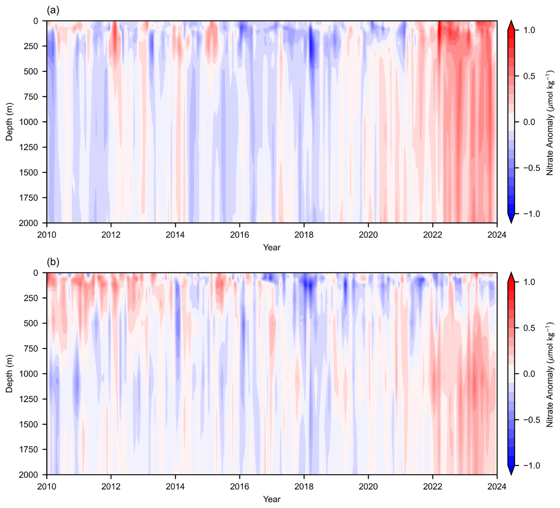
Figure 11 Interannual anomaly profiles of reconstructed nitrate concentrations in the MED (a) and NEA (b).

This study identifies three significant temporal trends. Firstly, there is a discernible overall increase in nitrate concentrations that is characterized by more frequent positive anomalies, particularly since 2021. This trend indicates an increasing fluctuation in nitrate levels and an escalation in eutrophication within the study area. The reconstruction outcomes align closely with trends observed in various case studies and extend these observations by providing results on a broader scale with more detailed quantification.

The MED exhibits a notably regular upward trend. BGC-Argo sequence analyses from the Sicily Channel revealed a slightly negative nitrate trend from 2011 to 2016, shifting to a positive trajectory thereafter until 2020 (Fourrier et al., 2022). In simulations employing physical–biogeochemical models under Representative Concentration Pathway (RCP) 4.5 and 8.5 scenarios for the northwestern MED, nutrients displayed a general ascending pattern that was notably more pronounced in deeper ocean layers than in surface waters (Reale et al., 2022). Remarkably, an anomalous nutrient surge after 2022 could potentially be linked to the severe winter storm Carmel in 2021. A detailed time series analysis over 4 years at the Levantine basin site demonstrated substantial replenishment of marine nitrates during the 2021 winter storm, reversing a declining trend that began in 2018 (Ben-Ezra et al., 2024). By contrast, interannual anomalies in the NEA are significantly more volatile. Although certain hypotheses suggest that intensified ocean stratification due to climate warming could limit nutrient availability in the upper-ocean layers, recent findings indicate that this limitation primarily affects phosphates, whereas nitrates continue to exhibit frequent and pronounced local fluctuations. The reconstruction results provide meticulous trend characterizations consistent with documented positive anomalies observed in the NEA's upper-ocean layers between 2010 and 2014 (Macovei et al., 2019), together with the identified growth patterns within the Iberian upwelling system (Padin et al., 2020).

Secondly, while vertical consistency of nitrate anomalies is stronger in the MED compared to the NEA, a decline in upper-ocean nitrate concentrations is evident in the NEA. Ocean warming has hindered the upward transport of nutrient-rich cold water, modifying the vertical nitrate distribution in the NEA. Moreover, no consistent overall trend of anomalies is apparent in surface nitrate concentrations in the NEA, which may be driven by complex ocean–atmosphere interactions and anthropogenic influences. Thirdly, the transition period of nitrate anomalies appears to be lengthening. The duration of individual positive or negative anomalies has extended from a few months at the beginning of the study period to several months or even over 1 year. This lengthening may indicate irreversible shifts in the marine environment or a decline in the ocean's self-regulatory capacity.

Furthermore, interannual anomaly trends must be interpreted cautiously due to their dependence on SSEVs and specific weights of the model, and their reliability requires further research. For instance, the reconstructed results may overestimate anomalies in the bathypelagic zone (>1000 m). At these depths, nitrate concentrations are relatively stable (Fig. 10) and are not effectively represented by SSEVs. Nonetheless, the model's estimates are inevitably influenced by the SSEV signal. The accuracy of these anomalies is significantly influenced by both the generalization capacity of the model and the stability of the input features. Despite the model's proven reliability, particularly with the MEB performance most relevant to anomaly calculations consistently maintaining an excellent level of ±0.04 µmol kg⁻¹ across multiple validations, small-scale findings still require further corroboration through targeted case studies. Overall, compared to the limitations posed by the discontinuous discrete observations from BGC-Argo and the inadequacies of simulated nitrate in capturing fine-scale variability, the reconstructed dataset offers an encouraging and comprehensive perspective for trend analysis.

3.6 Contribution of features to the model output

The current model is established based on all available features in the dataset, but given the redundancy among these features, the model may require fewer of the most efficient features. There are two benefits to entering all of the mentioned features. The ability of the MLP to automatically extract features ensures that the model will be enhanced and minimally affected by feature redundancy. In particular, the utilization of large-scale simulated nitrate data has significantly contributed to the model's ability to capture nonlinear relationships between multiple features, thus enabling it to effectively monitor nitrate concentration across a wide range of SSEV scenarios. On the other hand, analyzing the importance of each feature based on the model with all of the input features is crucial for further studies of nitrate estimation.

Figure 12 depicts the Pearson correlation coefficients among the features. Nitrate has been found to be positively correlated with depth and Chl and negatively correlated with SST (Yu et al., 2022). Furthermore, nitrate is positively correlated with features such as colored dissolved material (CDM), normalized fluorescence line height (NFLH), and 10 m wind speed (S10) and negatively correlated with features such as bottom euphotic layer depth (ZEU), heated layer depth (ZHL), and Secchi disk depth (ZSD). The spatial distribution is characterized by a positive correlation with latitude and a negative correlation with longitude, since nitrate concentrations in the NEA are generally higher than in the MED. Diverse relationships between the input features suggest the potential for feature redundancy, as exemplified by the marked positive correlation between SST and ZHL and the negative correlation between ZSD and Chl. The correlation coefficient can only capture linear relationships between variables, while MLP is a model to fit nonlinear relationships. Therefore, the contribution of features to the results cannot be determined solely based on correlation coefficients. The contributions of features based on SHAP values are discussed next.

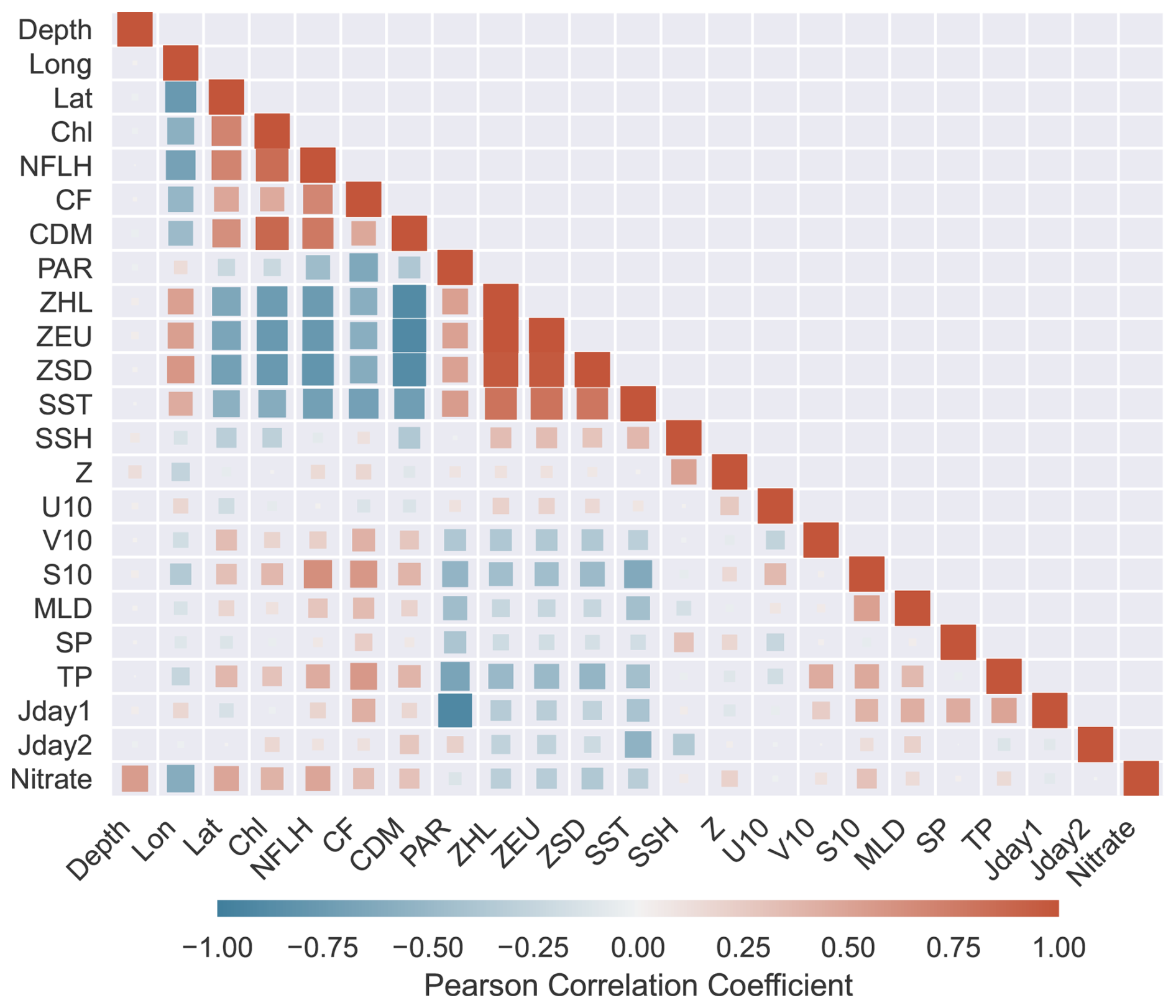
Figure 12 Heatmap for the matrix of Pearson correlation coefficients between nitrate and input variables. The size of the cell represents the absolute value of the correlation coefficient.

Given the high computational cost of SHAP (Chau et al., 2022) and the sufficient representativeness of a smaller sample (Pauthenet et al., 2022), we randomly selected 200 000 samples to estimate feature contributions. Figure 13 illustrates the probability distribution of the SHAP values for each feature, with the features ranked according to their average ASV. Given the different mechanisms by which the features affect the ocean at various depths, it is divided into two layers in the contribution discussion. Bounded by 200 m depth, the upper layer is the epipelagic zone (EZ), and the deeper layer of 200–2000 m is the mesopelagic zone and part of the bathypelagic zone.

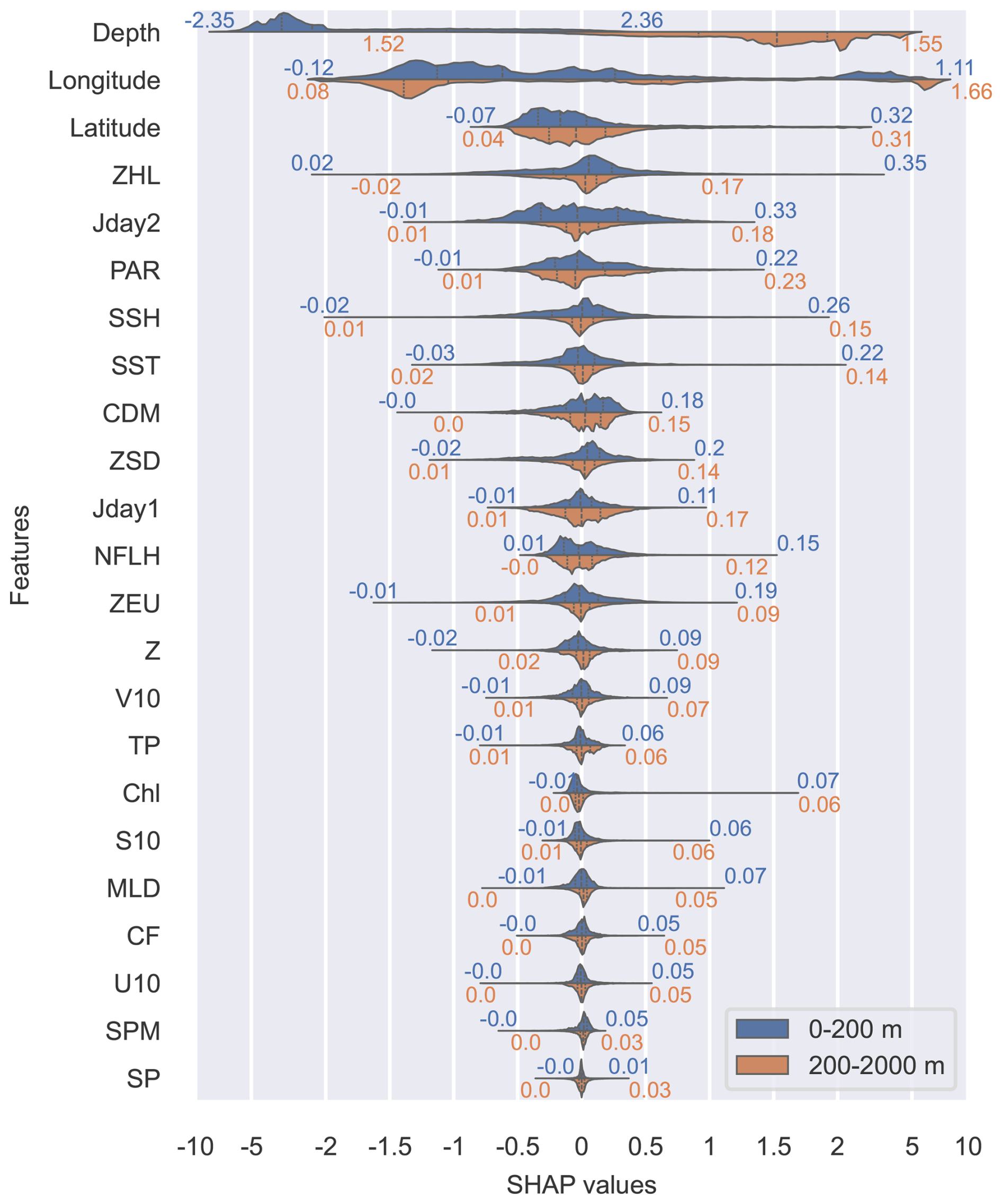
Figure 13 Probability distribution of SHAP values representing the impact of each feature on the model output. The y axis shows the input features, sorted by the total magnitude of I_j​, while the shaded area in the x-axis direction represents the distribution of the SHAP values, scaled due to the wide range. The numbers on the left show the mean of the raw SHAP values, while those on the right show the mean of the ASV. The black vertical dashed lines represent the median and quartiles of the SHAP values.

The input spatial features include depth, longitude, and latitude. Of these, depth is consistently identified as the strongest feature extracted by the model, which corresponds to the pattern of variations in the vertical distribution of nitrate, as depth uniquely facilitates the mapping of nitrate profiles (Fig. S3). Particularly in the EZ, the contribution of depth features is extremely significant, with $I_{\mathrm{Depth}}^{\mathrm{EZ}}=\mathrm{2.36}$, surpassing that of other features and by far that of the contribution at depths of 200–2000 m. This is attributed to the fact that the increase in nitrate concentration with depth is most pronounced in the EZ. The nitrate concentration at 200 m depth may be several times higher than that at the sea surface. Although such a trend is also observed at depths of 200–2000 m, the magnitude of this change is relatively small. Hence, depth always remains the most crucial feature, especially in the EZ.

Furthermore, longitude is the second essential feature in the model. Nitrate concentration in the MED and NEA differs greatly, resulting in longitude being more vital than latitude. At 200–2000 m depths, the contribution proportion of spatiotemporal coordinates increases, while the contributions of other SSEV features decrease. On the one hand, nitrate concentration in the surface ocean is more susceptible to SSEVs. On the other hand, nitrate in the deep ocean exhibits low seasonal variability but stable regional characteristics, and its concentration is primarily related to its location. The estimation process in the deeper ocean mainly relies on spatiotemporal coordinates supplemented by subtle adjustments to environmental variables.

The feature ranking in Fig. 13 aligns closely with that in Table S1 in the Supplement, though there are some minor differences. Both discuss the importance of features, but the SHAP values in Fig. 13 focus on the contributions of features, while the RMSE changes in Table S1 emphasize the irreplaceability of the features. For example, Z (total terrain depth), which provides a unique perspective, has a small contribution but significantly impacts the model when excluded. Furthermore, when excluding features, we combined Jday1 (the cosine function of the Julian day) and Jday2 (the sine function of the Julian day), which have a high contribution but a minimal impact on model performance when excluded. This is because Jday is a heuristic feature that, while useful for providing temporal information, can be inferred through the periodic variation of other variables. Figure 12 shows the correlation heatmap between nitrate and all of the input variables. The current feature combination is sufficient and potentially redundant; some highly correlated features can substitute one another to some extent, which is why the RMSE increase after excluding high-contribution features like photosynthetically available radiation (PAR) is relatively small. However, the comparison experiments in Table 1 confirm that the model can accommodate these correlated features and enhance their performance.

The residual features comprise environmental parameters, which encompass diverse facets of climate, biology, and ocean dynamics. Of these parameters, SSH exhibited a notably higher I_j value and demonstrated the most significant impact on model performance when excluded (Table S1). SSH reflects various dynamic effects of ocean circulation, mixing layers, and eddies, which together influence the horizontal and vertical transport of nitrates (Ascani et al., 2013; Fripiat et al., 2021; Sarangi and Devi, 2017; Wang et al., 2021). SSH reflects the influence of ocean dynamic variability on nitrate concentrations, typically exhibiting opposing impacts between the EZ and the deeper ocean.

Another set of critical features comprises SST-related variables. SST exhibits strong correlations with ZHL, PAR, and ZSD (Fig. 12), each concurrently presenting high I_j values and underscoring the dominant role that SST-related features play in nitrate estimation processes. Highly correlated features may dilute their individual contributions to the results, and SST may therefore play a more significant role than depicted in Fig. 13.

Previous studies have established SST as a principal environmental factor in nitrate retrieval, highlighting the fact that upwelling and winter convective mixing constitute two crucial physical processes that drive the transportation of cold, nitrate-rich waters into the euphotic layer, thereby boosting SSN and simultaneously reducing SST (Kudela and Dugdale, 2000; Pan et al., 2018). Since SST and SSH provide information on vertical mixing, their contribution in the deep ocean remains significant compared to other SSEVs. Of these, ZEU, PAR, NLFH, and CF are indicative of the optical environment, which is probably related to the oxidation of nitrogen by light inhibition and the activity of phytoplankton (Hutchins and Capone, 2022; Zakem et al., 2018). Furthermore, ocean dynamic parameters (e.g., MLD and S10) contribute to nitrate estimation by influencing nutrients in multiple ways (Tuerena et al., 2019; Liu et al., 2019).

Notably, Chl has previously been employed as another pivotal variable for SSN retrieval (Goes et al., 1999; Pan et al., 2018; Sarangi and Devi, 2017). However, in the EZ and the deeper layers, its average contribution remains relatively low, exhibiting instead a distribution characterized by a long tail of positive values. This phenomenon aligns closely with feature assessments of nitrate reconstruction in the Indian Ocean (Yang et al., 2024) and dissolved organic nitrogen studies in the Atlantic Ocean (Altieri et al., 2016). The predominant limiting factor is the confined spatiotemporal scope; although Chl is intrinsically linked to nitrate, its positive contributions are restricted primarily to vertical biologically productive upper layers and horizontally confined nutrient-rich regions, which only comprise a small portion of the oceanic 3D field. Consequently, regions minimally influenced by Chl dilute the average contribution of phytoplankton across broader oceanic estimations. Figure 14 illustrates the distribution of Chl contributions across specific samples. In the majority of cases, low chlorophyll concentrations yield negligible effects, while slight increases in Chl typically exert a negative influence, as phytoplankton growth consumes available nitrates (Goes et al., 2000). Conversely, exceedingly high chlorophyll levels significantly enhance nitrate estimation, potentially signaling eutrophication events. Furthermore, during training, the model seemingly captures more valuable Chl-related information from alternative features such as CDM, redistributing Chl's overall contribution to 3D nitrate estimations.

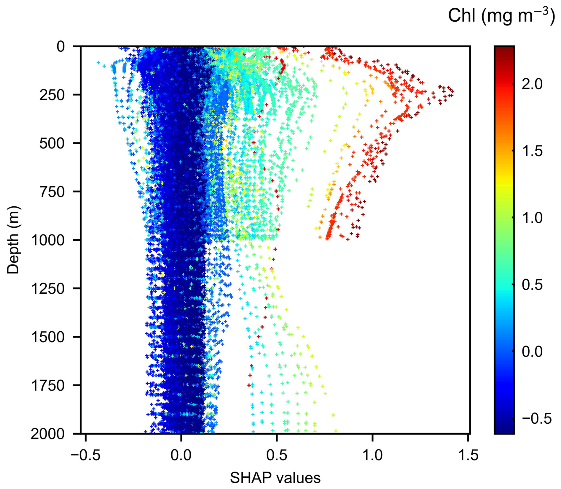
Figure 14 Scatterplot of Chl contribution values across the data samples. The x axis represents SHAP contribution values, while the y axis represents depth. The colors of the scatter points indicate the Chl feature values in each sample.

As described above, the SHAP approach can explain the effect of each feature on the MLP output from both holistic and individual perspectives. This approach enables comprehension of the role played by features in deep-learning black-box models. The ASV distribution of most features exhibits a long tail (Fig. 13), suggesting that even features with a low I_j can have a significant impact on model estimation in extreme environments. Nevertheless, the SHAP contribution is solely based on mathematical models and data-driven interpretations, which may result in conclusions that deviate from physical processes. Although it has been confirmed experimentally that removing features with a lower I_j results in less decline in model accuracy, the evaluation of the features still requires caution.

4 Data availability

The reconstructed 3D nitrate concentration dataset presented in this paper can be accessed via Zenodo at https://doi.org/10.5281/zenodo.14010813 (Yu et al., 2024). Here we provide a nitrate concentration gridded product for the pan-European ocean at 0.25°×0.25° horizontal resolution at 63 vertical levels from 0 to 2000 m and at a monthly resolution from 2010 to 2023.

5 Code availability

All the code used in the current study is available from the corresponding author upon reasonable request.

6 Conclusions

This study developed a continual-learning-based MLP model tailored to estimating the 3D ocean nitrate concentration. The model was cross-validated by independent in situ data profiles and demonstrated satisfactory performance, achieving an R² of 0.98, a RMSE of 0.592 µmol kg⁻¹, and a MAE of 0.398 µmol kg⁻¹. It also exhibited robust and reliable performance in both site-based cross-validation and independent cruise observations. Contrasting experiments show that the model's generalization is notably enhanced by employing continual learning from simulated nitrate, especially in regions with limited data availability. The estimation accuracy generally remains stable across all dimensions, with the more significant error occurring within the vertical range of 60–100 m and in the sparse region of the observations.

The 3D spatiotemporal distribution of nitrate is analyzed based on the reconstruction results. The findings indicate a progressive increase in oligotrophy from the western to eastern regions of the study area. Nitrate concentration shows significant seasonal variability in the vertical dimension driven by seawater exchange and biological processes. From an interannual perspective, a discernible increase in nitrate concentrations was noted, especially since 2021. In addition, vertical consistency in interannual anomalies within the NEA was lacking, with discrepancies commonly observed around depths of 100 and 500 m.

The contribution of each feature is calculated to gain insight into their influence on nitrate estimation. The results reveal that spatial coordinates such as depth, longitude, and environmental variables represented by SSH and SST exert the most significant influence. Meanwhile, certain features with low average contributions can still play vital roles in specific instances involving high anomalies.

The model still has certain limitations that require further improvements. Although its generalization ability has been enhanced, the nitrate distribution and trends in data-sparse regions should still be evaluated with caution. Due to the sparsity of BGC-Argo and the computational cost of CL, the model is limited to reconstructing water column profiles without incorporating large-scale spatiotemporal global features, which may prevent it from fully leveraging the potential of deep-learning models. The structure of the CL strategy imposes strict requirements on the datasets used for the two-stage training and may be affected by multiple sources of uncertainty, highlighting the need for higher-quality datasets in the future. Additionally, the current CL approach may introduce potential disturbances and performance fluctuations in regions with extensive BGC-Argo sampling. Future improvements could mitigate this limitation through dynamic weight parameters or additional modules.

From future perspectives, integrating remote sensing with deep learning to estimate oceanic 3D conditions has significant research potential. Continual learning allows for the incorporation of numerical model knowledge to address the limitations of sparse in situ measurements and can be coupled to any deep-learning model, making it a promising paradigm for reconstructing ocean datasets. Given the challenges of continuous high-resolution ocean monitoring, this approach can serve as an alternative solution to bridge the observation gap. Leveraging remote sensing expands retrieved variables and adds vertical dimension insights, supporting further research into the marine environment.