Oceanographic monitoring in Hornsund fjord, Svalbard

Several climate-driven processes take place in the Arctic fjords. These include ice–ocean interactions, biodiversity and ocean circulation pattern changes, and coastal erosion phenomena. Conducting long-term oceanographic monitoring in the Arctic fjords is, therefore, essential for better understanding and predicting global environmental shifts. Here we address this issue by introducing a new hydrographic dataset from Hornsund, a fjord located in the southwestern part of the Svalbard archipelago. Hydrographic properties have been monitored with vertical temperature, salinity and depth profiles in several locations across the Hornsund fjord from 2015 to 2023. From 2016 onward, dissolved oxygen and turbidity data are available for the majority of casts. The dataset contributes to the so far infrequent observations, especially in spring and autumn, and extends the observations, typically concentrated in the central fjord, to the areas adjacent to the tidewater glaciers. Because sediment discharge from glaciers and land is an inseparable part of the glacier–ocean interactions, the suspended sediment concentration in the water column and the daily sedimentation rate adjacent to the tidewater glaciers are monitored with regular water sampling and bottom-moored sediment traps. Here we present the planning and execution of the monitoring campaign from the collection of the data to the postprocessing methods. All datasets are publicly available in the repositories referred to in the “Data availability” section of this paper.

1 Introduction

1.1 Hydrographic and climatic conditions in the West Spitsbergen fjords

Hornsund is the southernmost fjord in Spitsbergen, the largest island of the Svalbard archipelago (Fig. 1a). The climate and hydrographic conditions in the fjord are strongly influenced by the topographically steered West Spitsbergen Current and the warm Atlantic Water it transports northward along the West Spitsbergen shelf break (Saloranta and Svendsen, 2001; Schauer et al., 2004). The heat loss from the West Spitsbergen Current to the atmosphere and surrounding water masses keeps the continental shelf west of Spitsbergen ice free. This results in warmer and more humid conditions compared to the northeastern part of Svalbard, which is influenced by Arctic air masses and sea ice cover.

On the West Spitsbergen shelf, the Sørkapp Current transports cold and fresh Arctic waters and sea ice around the southern cape of Spitsbergen (Fig. 1a). The polar front between these waters of Arctic origin and the warm West Spitsbergen Current centered on the slope restricts direct intrusion of the pure Atlantic Water into the fjords (Saloranta and Svendsen, 2001). Large-scale atmospheric forcing and Ekman transport can, however, cause the Atlantic Water transported by the West Spitsbergen Current to flood onto the West Spitsbergen shelf and mix with the Sørkapp Current (Nilsen et al., 2016; Goszczko et al., 2018). The mixing with waters of Arctic origin results in modified or transformed Atlantic Water. It is this modified Atlantic Water that is most often observed in the fjords and therefore generally responsible for potential heat transport toward the glacier termini (Svendsen et al., 2002; Nilsen et al., 2008; Promińska et al., 2017; De Rovere et al., 2022).

Calving rates at tidewater glaciers in the West Spitsbergen fjords have been shown to increase with increased seawater temperatures (Luckman et al., 2015; Holmes et al., 2019; van Pelt et al., 2019; Błaszczyk et al., 2023). As the Arctic continues to warm, accelerated frontal calving as well as enhanced surface and submarine melt from marine-terminating glaciers increases freshwater and sediment discharge into the fjords. Consequently, the vertical stratification, optical properties, nutrient availability and chemical composition of seawater are changing (Murray et al., 2015; Moskalik et al., 2018; Błaszczyk et al., 2019). Because the Arctic and Atlantic waters host different species of zooplankton and fish, the changing environment has potentially prominent consequences for marine ecosystems in the West Spitsbergen fjords (Meire et al., 2017; Hopwood et al., 2020; Trudnowska et al., 2020; Stempniewicz et al., 2021).

1.2 Recent changes in the hydrography of the West Spitsbergen fjords

Compared to the other West Spitsbergen fjords, oceanographic studies from Hornsund are still limited. More comprehensive observations and analyses are available from the more northern fjords, i.e., Isfjorden and Kongsfjorden (Fig. 1a). Studies from Isfjorden and Kongsfjorden indicate that the intrusion of Atlantic-derived waters, typically first observed in mid-June after the geostrophic control between the fjord and shelf waters has weakened, reaches its maximum volume inside the fjord as late as September (Svendsen et al., 2002; Cottier et al., 2005; Nilsen et al., 2008; Pavlov et al., 2013). In recent years, warming of both the atmosphere and ocean has led to reduced ice formation and decreased production of dense Winter Cooled Water with temperature below −0.5 °C and salinity over 34.4 (Muckenhuber et al., 2016; Tverberg et al., 2019). Consequently, the horizontal density gradient between the West Spitsbergen fjords and the shelf has weakened, allowing the warm shelf waters to penetrate into the fjords (Tverberg et al., 2019). Simultaneously, atmospheric forcing during winter has become more favorable for the flooding of Atlantic Water and less favorable for the presence of the Arctic Water on the West Spitsbergen shelf (Nilsen et al., 2016; Goszczko et al., 2018; Strzelewicz et al., 2022). Together, these changes have enabled larger volumes of the waters with Atlantic origin to be more frequently observed in Isfjorden and Kongsfjorden, especially during winter (Cottier et al., 2007; Nilsen et al., 2016; Tverberg et al., 2019; Skogseth et al., 2020; De Rovere et al., 2022). Strzelewicz et al. (2022) did not identify a trend in the presence of Atlantic waters in Hornsund, although they noted a decrease in the presence of Winter Cooled Water. Their results were, however, based on a single transect acquired during summer. Overall, a majority of the studies focusing on the hydrography of Hornsund are based on observations obtained in July. This leaves seasonal changes in hydrographic conditions undetected; therefore, the full extent of Atlantic heat import may not be captured. In addition, analysis based on such temporally limited datasets causes a risk of interpreting temporal shifts in the seasonal cycle as artifacts of interannual variability.

Another shortcoming of the regular observations that are available for Hornsund is that they are concentrated merely in the central fjord, ignoring the complex shoreline of Hornsund (Fig. 1c). Consequently, the seasonal and interannual variabilities of hydrographic conditions in the inner basins that are directly influenced by tidewater glaciers remain unexplored. The bathymetric sills at the entrance of the inner bays (Fig. 1c) potentially delay or restrict the influence of intruding Atlantic waters and hence the heat flux to the glacier termini (Nilsen et al., 2008; Arntsen et al., 2019). Arntsen et al. (2019) used mooring data at a sill of Brepollen, the largest and innermost bay in Hornsund, to study the controls of the inflow of warm Atlantic waters and their influence on the tidewater glaciers. Their analysis covered two contrasting winters: (1) 2010–2011, when waters at the sill were relatively cold, and (2) 2013–2014, when warmer waters were present. They concluded that the wind stress, coastal trapped waves and tides are the important mechanisms governing the cross-sill transport of water masses from the main basin to Brepollen. In addition, by studying marine-terminating glaciers in western Spitsbergen, Holmes et al. (2019) showed that measuring temperature in the waters directly in contact with (or as close as possible to) the glacier is essential for correctly estimating the impact of the oceanic heat flux on frontal ablation.

1.3 General concept of the long-term oceanographic monitoring of Hornsund fjord

In order to address the need for more extensive seasonal and areal coverage of hydrographic observations, the Institute of Geophysics Polish Academy of Sciences (IG PAS) initiated a campaign for the long-term oceanographic monitoring of Hornsund, the so-called LONGHORN program. Hydrographic surveys, consisting of vertical salinity and temperature profiles, have been carried out since 2015. From 2016 onward, most of the profiles include measurements of dissolved oxygen and turbidity as well. The design of the surveys takes into account the complex shoreline characteristics of Hornsund by covering areas close to the glacier termini as well as the central basin. With increasing freshwater discharge from glaciers and land, the coastal waters are receiving more terrestrial matter (Zhang et al., 2022). Therefore, in addition to the hydrographic observations, the monitoring includes regular measurements of suspended sediment concentration and sedimentation rate. By quantifying the amount of organic matter in the sediment samples, the data also allow for monitoring changes in biological production. The surveys contribute to the availability of observations over spring, summer and autumn seasons. Here we present data collected until 2023. However, the monitoring program is still ongoing, and its aim is to build a long-term dataset.

In Sect. 2, we present the study area, Hornsund fjord, and its distinct characteristics compared to the other West Spitsbergen fjords. In Sect. 3, we outline the monitoring campaign by reviewing the practical arrangements for fieldwork, including logistical challenges and the instruments used for measurements. We also give an overview of the temporal and spatial coverage of the dataset. In Sect. 4, we describe the methods used for data processing, including procedures for compression and quality control of the collected data. Finally, in Sect. 5, we present selected preliminary findings to highlight the benefits and importance of the dataset.

Figure 1 (a) Svalbard archipelago and the location of Hornsund fjord framed with a black box; locations of Kongsfjorden (KF) and Isfjorden (IF) are indicated. The major currents the West Spitsbergen Current and the East Spitsbergen Current are shown with red and blue arrows, respectively. The polar front separating them is marked with a dashed gray line. The currents and the front are based on Saloranta and Svendsen (2001) and references therein. (b) Station plan for Hansbukta. The zoomed-in area is indicated as a gray rectangle in panel (c). The yellow star denotes the location of the Polish Polar Station Hornsund (denoted PPS). The bathymetric scale is the same as in panel (c). (c) Map of Hornsund area with locations of CTD stations included in the hydrographic survey. White dots indicate locations of the core stations since 2022. Black dots indicate the supplementary CTD stations and the locations of the core stations before 2022. Bathymetric data are based on the Norwegian Hydrographic Service, Moskalik et al. (2013) and Ćwiąkała et al. (2018). Note that the bathymetric data close to the glaciers are missing. Landsat-9 image (taken on 27 July 2023), courtesy of the U.S. Geological Survey.

2 The study area

Hornsund is a shallow fjord with a maximum depth of 240 m and length of 35 km. There is no bathymetric sill between the approximately 8 km wide fjord mouth and the West Spitsbergen shelf, but, on the other hand, there is no deep connection either (Fig. 1c). Despite its southern location in the Svalbard archipelago, Hornsund is less influenced by the Atlantic waters than, for example, the more northern Isfjorden and Kongsfjorden (Nilsen et al., 2016; Promińska et al., 2017). One reason behind the greater isolation of Hornsund is the much shallower, about 200 m deep, entrance compared to the other West Spitsbergen fjords. Another factor contributing to the lesser presence of Atlantic waters in Hornsund is the more pronounced polar front separating the warm West Spitsbergen Current and the colder Sørkapp Current on the southern West Spitsbergen shelf (Saloranta and Svendsen, 2001; Promińska et al., 2018).

Hornsund has complex geometry with several inner bays, also called fjord arms, characterized by marine-terminating glaciers (Fig. 1c). Of the total surface area, approximately half consists of these smaller bays, which used to be almost entirely covered by glaciers in the beginning of the previous century (Błaszczyk et al., 2013). Błaszczyk et al. (2013) estimated that between 2001 and 2010 glaciers in Hornsund retreated with an average rate of 70 m per year, while the average retreat for glaciers in Svalbard during the same period was 45 m per year. Still today, Hornsund is heavily glaciated, which, together with the more restricted input from the West Spitsbergen Current, leads to higher freshwater flux and lower salinity compared to the other West Spitsbergen fjords (Promińska et al., 2017; Błaszczyk et al., 2019).

The five fjord arms – Hansbukta, Vestre Burgerbukta and Austre Burgerbukta in the north, Brepollen in the east, and Samarinvågen in the south (Fig. 1c) – are separated from the main basin by shallow sills originating from glacial deposits of moraines; therefore, the warm and deep inflows into the main basin of Hornsund may only have a limited influence on the glacier termini (Arntsen et al., 2019). It has been observed that the Winter Cooled Water typically persists in the deep depressions of the bays long into the summer; hence, the bays can be regarded as an archive of conditions prevailing during the previous winter (Promińska et al., 2018; Skogseth et al., 2020).

The monthly mean air temperature in Hornsund varies from −10 °C in winter and early spring to almost 5 °C during summer months (Wawrzyniak and Osuch, 2020). Since the 1970s, the annual mean air temperatures in Hornsund have increased by 1.14 °C per decade (Wawrzyniak and Osuch, 2020). The most pronounced warming has occurred during winter with approximately 4 °C increase between periods 1971–2000 and 2001–2015 (Isaksen et al., 2016). Observations of seawater temperature span a considerably shorter time and show large interannual variability. Based on summertime observations, an annual temperature increase of 0.03 °C was found for the period 2001–2015, but the trend was not statistically significant (Promińska et al., 2018).

3 The LONGHORN monitoring program

The oceanographic monitoring within the LONGHORN program is carried out by the Department of Polar and Marine Research at the Institute of Geophysics Polish Academy of Sciences (IG PAS) using the infrastructure of the Polish Polar Station Hornsund.

The monitoring consists of the following components:

• vertical CTD (conductivity–temperature–depth) profiles,

• vertical profiles of dissolved oxygen and turbidity (available for the majority of CTD casts),

• suspended sediment concentration with loss on ignition from water samples,

• daily sedimentation rate (sediment flux) with loss on ignition from bottom-moored sediment traps.

Each component of the monitoring program is discussed individually in the following subsections.

3.1 Hydrographic monitoring

Initially, the hydrographic monitoring program consisted of over 50 standard CTD stations, with along- and across-fjord sections in the main basin and in all the inner bays (Fig. 1). In addition, between 2015 and 2018 Hansbukta was intensively surveyed with another approximately 50 stations related to separate research projects. However, the data collected during the first 4 years indicated that having such a densely spaced measurement plan was not necessary to resolve the horizontal variability in Hornsund (Fig. 2). In addition, visiting that many stations regularly was time-consuming. Therefore, from 2019 onward, the number of stations was reduced to 16. From 2022 onward, the survey has consisted of 11 stations: one in the center of the fjord, one in Brepollen, one in Gåshamna and two stations in each of the other bays, i.e. Samarinvågen, Austre Burgerbukta, Vestre Burgerbukta, and Hansbukta (Fig. 1c and Table 1). Of the two stations in the major fjord arms, one is located in the center of the bay and the other one is close to the glacier front.

The locations for the new stations since 2022 were chosen as the deepest points in the main fjord and in the inner bays. Therefore, their positions somewhat differ, at most 1.5 km, when compared to the stations from the initial phase of the monitoring program (Table 1). Nevertheless, we chose to not rename the stations as the horizontal variability even over larger distances was found to be negligible. An example of horizontal variability in Vestre Burgerbukta, where the distance between the old and new locations of station BuBW_01 was the largest (Table 1), is shown in Fig. 2. The stations close to the glacier front are located approximately 500 m from the edge of the glacier, equidistant from the shorelines. The distance to the glacier front was measured with a Bushnell Tour V5 laser rangefinder. Due to the retreating glaciers, the locations of these stations are not stationary but change seasonally and interannually. Their positions shown in Fig. 1c are based on single, randomly chosen, measurements obtained during 2022.

The 11 stations measured from 2015 to 2023 are the core stations of the hydrographic monitoring program. The rest, about 100 stations, constitute the supplementary stations that were visited mainly during the initial stage of the monitoring program and intermittent campaigns related to various other research projects. Over one-third of the supplementary stations are located in Hansbukta. The supplementary stations are shown in Fig. 1b and c as black dots.

Naming of the core stations follows the convention where the first letters indicate the region, e.g., BuBE for Austre (East) Burgerbukta and HB for Hansbukta. The stations that are approximately 500 m from the glacier edge get the first letter from the name of the glacier, e.g., PG stands for Paierl glacier (Paierlbreen), with capital G standing for glacier.

Table 1 List of core CTD stations included in the hydrographic monitoring. In 2022, stations were relocated, and the distance indicates the difference between the past and present positions. In addition, new stations 500 m from the glacier termini were introduced. It should be noted that the positions of these stations are not fixed. The stations where there was regular monitoring of suspended sediment concentration and daily sedimentation rate are in bold.

^a These stations are located 500 m from the glacier termini; therefore, the position is changing with glacier retreat/advance. The coordinates are chosen randomly from data collected in 2022. The bottom depth is given as minimum to maximum depths. ^b Station GH_01 was introduced to the monitoring program in 2021.

Figure 2 Salinity (a) and temperature (b) profiles displaying the modest horizontal variability of hydrographic properties within Vestre Burgerbukta. Stations BuBW_01 (solid line) and BuBW1_04 (dotted line) are shown for Vestre Burgerbukta. The distance between the two stations is 2200 m, with BuBW_01 being closer to the glacier front. Two different years (2017 and 2018) with observations covering several months are shown.

3.1.1 Description of the CTD instruments

Different instruments, two SAIV A/S SD208 STD¹/CTD profilers and one Valeport miniCTD, are used for the CTD surveys. All instruments directly measure pressure, in situ temperature and conductivity. In 2015, all observations were made with the Valeport miniCTD, but since 2016, the SAIV A/S SD208 CTD has been the most commonly used instrument as, in addition to temperature and conductivity, it includes sensors for turbidity and dissolved oxygen. In July 2018, the SAIV A/S SD208 CTD instrument was lost, and measurements until the following June were carried out with the Valeport miniCTD. A new SAIV A/S SD208 CTD has been the main device for hydrographic monitoring since June 2019.

The SAIV A/S SD208 CTD instrument is programmed to measure with a frequency of 0.5 Hz. In 2016, the first year the sensor was used, a higher sampling rate of 1 Hz was applied, but this compromised the auto-scale settings of the turbidity sensor. Thus, it was decided to decrease the sampling frequency. The Valeport miniCTD is typically programmed to measure with a frequency of 8 Hz. Other essential technical details of the CTD sensors are summarized in Table 2.

All instruments used to measure hydrographic properties were calibrated in the laboratory by their respective manufacturers before purchase. After this initial calibration, the instruments are intermittently compared against each other. Extensive intercomparisons of all instruments were conducted in September 2017, April 2018 and in August–September 2020. The results of the intercomparison revealed an offset in the conductivity readings of both SAIV A/S SD208 CTD profilers used in the hydrographic survey. The results of the intercomparisons are discussed in Appendix A.

Table 2 Instruments used in hydrographic monitoring and the directly measured variables (information obtained from the manufacturers). FTU represents formazine turbidity unit.

3.1.2 Collection of hydrographic data

The hydrographic monitoring is conducted by trained research personnel of the Polish Polar Station Hornsund from an outboard motorboat. To obtain a full-depth profile, the instrument is typically lowered all the way to the bottom. It should be noted that until summer 2016, due to the length of rope used, the maximum depth of casts was only 150 m; therefore, the bottom was not reached in some locations. The lowering speed is not intended to exceed 0.5 m s⁻¹. However, usually the rate of descent was manually controlled, and only occasionally was a winch with rope speed monitor available. Manual operation causes irregularities in the descent rate that are transferred to the sampling frequency per depth unit. The median lowering speed calculated from the raw data is 0.4 m s⁻¹ for SAIV A/S SD208. The highest median descent rate for a single profile was 0.9 m s⁻¹, and the highest instantaneous lowering speed reached 1.8 m s⁻¹.

Another potential source of inaccuracy caused by the measurement arrangement is the drift of the boat from the measurement point during the cast. In general, when considerable (over 100 m) drift from the fixed coordinate point is observed to occur, the cast is repeated after repositioning. The same 100 m distance is considered the maximum acceptable deviation from the fixed location set for the monitoring station. Therefore, the maximum error in the given position is considered to be less than 100 m. However, in addition to the drift of the boat, currents may cause a tilt in the rope due to the low weight of the instrument. Overall, the inaccuracies resulting from positioning or tilting are considered to be negligible because of the shallow depths and rather small horizontal differences in the water column structure in different parts of Hornsund fjord (Fig. 2).

3.1.3 Horizontal and temporal coverage of the dataset

Because of the polar night and weather and ice conditions, the timing of boat-based observations is limited to between May and October, although occasional observations during the polar night are also available. The availability of hydrographic observations from different areas of Hornsund fjord is shown in Fig. 3. The most comprehensive and frequent hydrographic observations have been obtained in Hansbukta due to its proximity to the Polish Polar Station Hornsund. Of the larger fjord arms, the most extensive dataset is obtained from Brepollen.

The desired interval for hydrographic measurements varies from 2 weeks for the stations close to the Polish Polar Station (Hansbukta, central fjord and Gåshamna) to 4 weeks for the other stations. However, the frequency with which each station is visited depends on weather and ice conditions as well as the availability of staff responsible for the observations. Consequently, the timing of observations varies between the years, and monthly observations are not available for each year or area.

Figure 3 Temporal coverage of CTD data. Dates of CTD casts obtained with the Valeport miniCTD are marked with diamonds, and casts obtained with the SAIV A/S SD208 CTD, equipped with turbidity and oxygen sensors, are shown with circles.

Figure 4 (a) Periods of sediment flux measurements. The circles connected with a line denote the time between sediment trap deployment and recovery. When no line is visible, the sediment trap was deployed for a short time (in general for 24 h). (b) Dates of water sampling for suspended sediment concentration. The circles denote dates when multiple depths in the water column were sampled for analysis of suspended sediment concentration. The triangles mark the dates when only a surface sample (0 m) was obtained.

3.2 Suspended sediment concentration and sedimentation rate

The LONGHORN monitoring program includes two core stations in contrasting environments for regular sediment sampling. Hansbukta (station HB_01 with a bottom depth of 88 m) receives freshwater and sediments from the marine-terminating Hansbreen, whereas Gåshamna (station GH_01 with a bottom depth of 31 m) is a shallow bay receiving river transport from Gåsbreen, the largest land-based glacier in Hornsund, and the surrounding terrain (Fig. 1c and Table 1). The aim is to obtain observations covering the period from May to October, but there is some variability in the start and end timing of the monitoring each year. In addition to the stations in Hansbukta and Gåshamna, occasional samples are available from the other fjord arms as well (Fig. 4).

Regular water sampling and sediment flux measurements at station HB_01 in Hansbukta began in 2016. In 2015, measurements were conducted slightly further from the glacier. For the first years of monitoring (2015–2018), suspended sediment concentrations are available from the section perpendicular to and also from the section parallel to the glacier front (Fig. 1b). Monitoring in Gåshamna started in 2021 with measurements on sediment deposition. Since 2022, both sedimentation rate and suspended sediment concentration are available from Gåshamna. It should be noted that the location of station GH_01 differs by 200 m between 2021 and 2022.

The water samples are collected with a Hydro-Bios FreeFlow 1 L Niskin bottle from multiple depths in the water column. The daily sedimentation rate is measured with a sediment trap consisting of two cylindrical tubes, with a diameter of 80 mm and volume of 1 L. The tubes are mounted on a gimballed frame moored to the seafloor. In order to keep the tubes oriented vertically, a submersible float is attached 5 m above the trap. During the first 3 years (2016–2018) of sediment flux measurements, the sediment traps were in general deployed above and below the pycnocline, i.e., 5–15 and 20–25 m from the surface. Since 2019, most of the measurements are obtained 5 m above the bottom. The material settled in the sediment traps was initially collected after 24 h, but since 2022, the sediment traps are deployed and recovered approximately every 10 d.

Typically, the whole 1 L water sample is filtered through Whatman GF/F 0.7 filters (diameter 45 mm) for the analysis of suspended sediment concentration. For samples from the sediment traps, partitioning of the 1 L sample is performed before filtration. Typically, $\mathrm{1}/\mathrm{4}$, $\mathrm{1}/\mathrm{8}$ or $\mathrm{1}/\mathrm{16}$ of the sample is filtered. Prior to filtration, the filters are dried in an oven at 200 °C for 2 h and then weighed on a 1.00×10⁻³ g precision scale. After filtration, the filters are dried at 40 °C for 24 h and then left in the desiccator before weighing. Sediment weight is obtained from the difference in the dry filter weight before and after filtration. To get the suspended sediment concentration, this mass is divided by the volume of the water sample used for filtration. The daily sediment deposition is calculated from the obtained sediment weight divided by the area of the tube and the duration of deployment.

As a final step, organic matter is incinerated by baking the filters in an oven at 550 °C for 3 h and then left in the desiccator before weighing. The loss on ignition (LOI) value is calculated as the difference in the weight of sediments before and after ignition divided by its weight before ignition. This value can be considered an estimate of the amount of organic matter in the sediment. The final dataset on sedimentation rate is available at https://doi.org/10.1594/PANGAEA.967172 (Moskalik et al., 2024c). It includes information on locations, deployment and recovery dates, deployment depths, sedimentation rates, and the LOI values. The dataset on suspended sediment concentration is found at https://doi.org/10.1594/PANGAEA.967173 (Moskalik et al., 2024d), with information on location, sampling date and depths, as well as concentration of total suspended particles and the LOI value.

4 Processing of CTD data

4.1 Removal of unrealistic values

The data recorded by the SAIV A/S SD208 CTD and the Valeport miniCTD are downloaded and converted into ASCII format with Minisoft SD200W and DataLog x2 software, respectively. Both software packages automatically apply their own routines to calculate thermodynamic variables (potential temperature, practical salinity, density and sound velocity) based on the directly measured variables (conductivity, in situ temperature and pressure). However, for consistency, all derived variables in the final processed dataset are calculated using the Gibbs SeaWater (GSW) Oceanographic Toolbox developed for MATLAB (McDougall and Barker, 2011). The GSW Oceanographic Toolbox implements The international thermodynamic equation of seawater – 2010 standard (TEOS-10; IOC et al., 2010). Following the recommendation of the TEOS-10 standard, salinity and temperature in the published datasets are practical salinity and in situ temperature. No absolute salinity or conservative temperature have been added to the datasets, and here salinity refers to practical salinity and temperature to in situ temperature. It should also be noted that the variables in the raw-data files are those derived by the software packages provided by the manufacturers of the instruments.

Automatic routines are applied to filter out salinity values lower than 20 and higher than 35.2. High-salinity spikes rarely occur, and almost all filtered values are unrealistically low and occur close to the surface or in the bottom layer when the sensor may be in contact with the bottom sediments. The suspiciously low salinity values are also associated with atypically large vertical gradients (>1 psu dbar⁻¹, where psu represents practical salinity unit on the Practical Salinity Scale, PSS-78) and mostly occur in early spring when there is practically no freshwater flux to the fjord. Because the low salinities occur when air temperature is below 0 °C and because they are only observed during the downcast, we assume that they result from ice formation in the sensor while the instrument was left on deck between measurements. In the bottom layer, the low salinities are also identified by reversed density stratification. In such cases, all bottom values are discarded.

The measured temperature is tested against the local freezing point temperature, and when the temperature is more than 0.1 °C below the freezing point, both temperature and salinity are removed. This typically occurs in the topmost surface layer in early spring when the air temperature is below 0 °C. The temperature below the freezing point is often associated with suspiciously low salinity, which supports our conclusion that the salinities below 20 result from ice formation in the conductive cell.

Occasionally, turbidity and oxygen sensors have shown spikes close to zero, likely due to a malfunction in the connective cables. These spikes are removed by setting a lower limit of 0.2 for turbidity and 65 % for dissolved oxygen saturation. These limits were chosen by visually inspecting all data outside the typical range and by detecting spikes in the vertical profiles. In general, turbidity does not exceed 150 FTU; therefore, all profiles showing higher values are visually inspected. The upper acceptable limit for oxygen saturation is set to 140 %. The upper limit is exceeded when the protective cap of the oxygen sensor is not removed before the cast. In addition to the high oxygen concentration, these casts can be visually recognized from rapidly increasing oxygen saturation with depth.

The turbidity and oxygen sensors are located at the base of the instrument; therefore, they may become submerged in the bottom sediments when the instrument is lowered. Because these are optical sensors, the high sediment concentration results in rapid beam attenuation and near-bottom peaks, especially in the downward-looking oxygen sensor. Such peaks are detected and removed.

4.2 Data compression

After deriving the thermodynamic variables as well as initial filtering of unrealistic values, the data are compressed to 1 dbar vertical bins. This is done by taking the median value of measurements within a half-unit distance from the center of the bin. Consequently, because the first bin is centered at a depth of 1 dbar, the measurements in the uppermost 0.5 dbar layer are not included in the final averaged data but can be found in the raw-data files. In general, both downcasts and upcasts are used in the median filtering for temperature and salinity as well as the thermodynamic variables. However, all profiles are visually checked, and occasionally the upcast profile is rejected because of values deviating from those of the downcast profile. This often occurs with data recorded by the Valeport miniCTD as the conductivity sensor is located at the base of the instrument and can therefore become clogged when in contact with bottom sediments. Of the salinity profiles obtained by the SAIV A/S SD208 CTD, less than 1 % of the upcasts are rejected. Considering the programmed sampling rate and estimated lowering speed of 0.4 m s⁻¹, the median for the SAIV A/S SD208 data is typically taken from three measurements when both downcasts and upcasts are included.

For turbidity and oxygen, typically only the downcast profile is included in the final median-filtered dataset, because possible bottom contact often leaves the optical sensors covered in sediments for a considerable part of the ascent. Despite this, occasionally both downcasts and upcasts or only the upcast have been used for turbidity and oxygen. This may be the case when the instrument has been lowered too fast and when the overall quality of the data could be improved by including the upcast. In addition, in a few cases the sensors may not have been adequately cleaned before the cast, which leaves the turbidity sensor, in particular, to display suspiciously high values during the downcast. In such cases, only the upcast has been considered. Nonetheless, before accepting the upcast profile, the data are always carefully visually inspected. Due to the low sampling rate of the SAIV A/S SD208 CTD, including only the downcast profile or upcast profile leaves, in general, only two measurements per 1 dbar vertical bin. Consequently, the bin average for turbidity and oxygen is typically formed from two measured values.

4.3 Final steps: smoothing and data archiving

Because of the relatively low number of measurements within one vertical bin, averaging based on median filtering does not necessarily remove individual spikes and outliers. Therefore, after linearly interpolating missing values, the data are smoothed using MATLAB's smooth function with a low-pass filter and a window size of four (moving average of four consequent depths). If less than 70 % of the data are available over the total depth, then interpolation is not performed, and the whole profile is rejected. Examples of raw data and the final median-filtered and smoothed data are shown in Fig. 5.

Before making the data publicly available in a data repository, the data are visually inspected for consistency by comparing groups of profiles selected according to area or timing of observation. The CTD data are divided into two datasets: one consisting of the core CTD stations and the other including all other supplementary stations. Both processed final datasets include the variables shown in Table 3. Conductivity is not included in the final 1 dbar-averaged datasets but can be found in the raw-data files. The core CTD dataset is available at https://doi.org/10.1594/PANGAEA.967169 (Moskalik et al., 2024a), and the supplementary dataset is available at https://doi.org/10.1594/PANGAEA.967171 (Moskalik et al., 2024b).

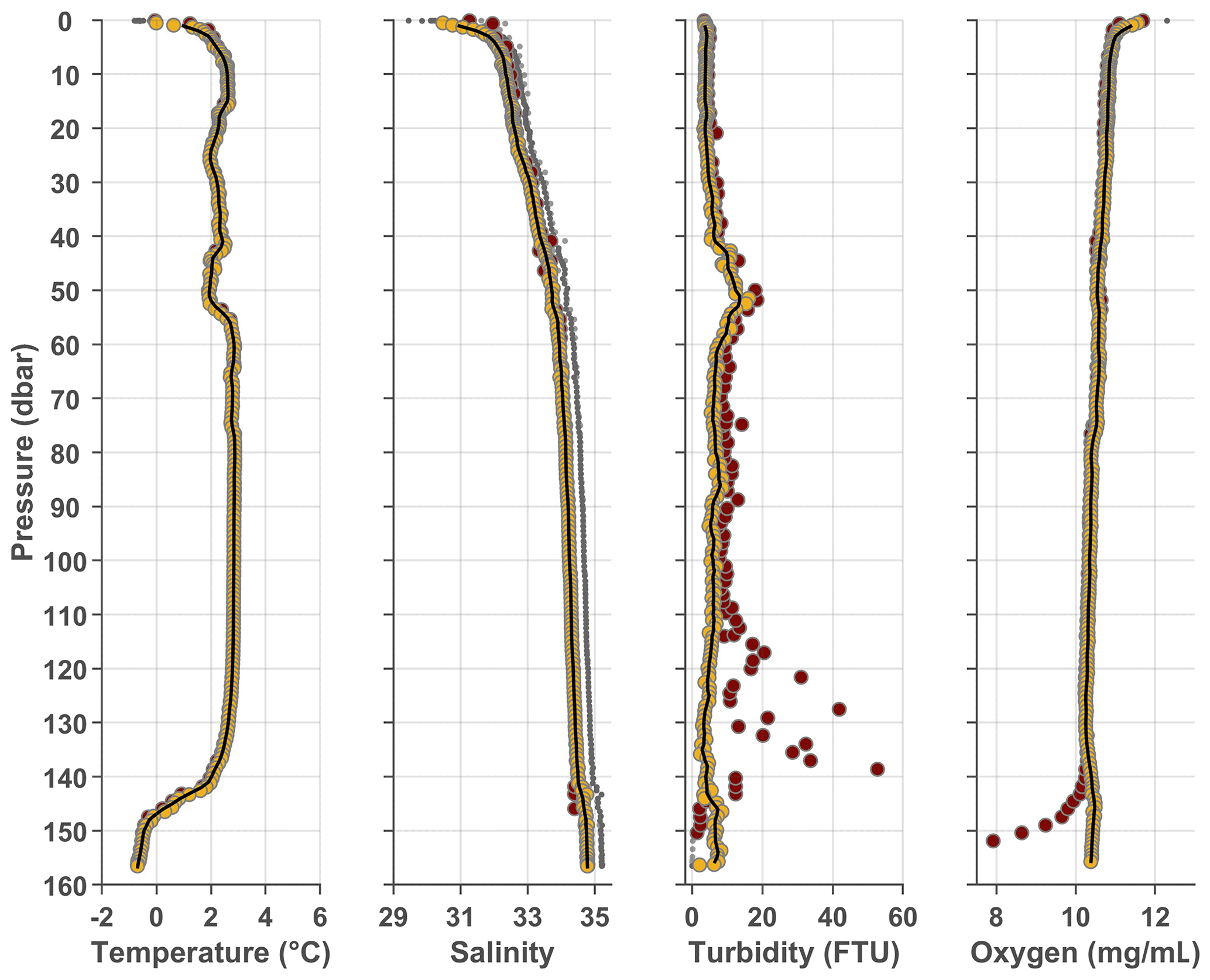
Figure 5 An example of processing the CTD data from station BuBW_01 on 20 September 2019. The raw data are marked with gray dots. The yellow and brown circles indicate the measurements taken during the downcast profiles and upcast profiles, respectively. The black line is the final data after averaging to 1 dbar vertical bins and smoothing. Note that for the profile shown here the upcast profile is rejected for turbidity and oxygen due to contact with bottom sediments.

Table 3 Variables in the final processed dataset for vertical CTD profiles. Additional metadata such as the used instrument and bottom depth can be found in the data repositories (Moskalik et al., 2024a, b).

^a Start time of the profile. Valeport miniCTD data only include date. ^b These variables are available for casts recorded by the SAIV A/S SD208.

Figure 6 Interannual variability of salinity (a) and temperature (b) in different basins in Hornsund fjord from 2015 to 2023. Average profiles for August each year are shown. Note that the data availability varies between basins, which results in missing data during some years.

5 Oceanographic data

5.1 Overview on hydrographic conditions in Hornsund

The hydrographic characteristics in the central Hornsund fjord in July have been extensively studied and described by Promińska et al. (2017, 2018) and Strzelewicz et al. (2022). The dataset introduced here adds to the current knowledge by extending the observations from the central fjord to the various fjord arms as well as by allowing for assessment of seasonal variability. One of the questions arising from the complex geometry of Hornsund is how the fresh and cold waters of glacial and terrestrial origin interact with the saltier and warmer waters from the West Spitsbergen shelf. The effect of the freshwater flux is seen in Fig. 6a, showing vertical salinity profiles obtained in August of each year (2015–2023). In the bays close to the glaciers, the surface salinity generally decreases below 31 during summer, whereas in the central fjord the surface salinity remains in a typical year above 31. Whereas the surface salinity is relatively stable between the years in the center of the fjord and in Brepollen, in the Vestre Burgerbukta and Austre Burgerbukta local processes seem to cause considerable interannual variability.

The fjord arms with a bathymetric sill are known to be archives of Winter Cooled Water formed as a result of ice formation during winter. While the temperature in the central fjord is over 2 °C (also in the deep layers), the bottom temperatures in all the larger fjord arms generally remain close to 0 °C even in August (Fig. 6b). In the upper layers, the temperatures in the bays typically reach 4 or 5 °C by August. The surface temperatures observed in the inner bays are comparable to the temperature in the center of the fjord.

Already the time series from 2015 to 2023 shows high interannual variability of hydrographic conditions in Hornsund. For example, in August 2015 the upper 50 m layer was especially cold in all regions (Fig. 6). In the following August 2016, the bottom layer was exceptionally warm in all basins with temperatures over 1 °C higher compared to the other years. The bottom waters in the Vestre Burgerbukta reached even higher temperature, exceeding 3 °C. Besides August 2016, 2023 was also warmer than average in the upper layer. However, in contrast to the relatively high surface salinities observed in 2016, the lowest salinities were observed in 2023.

Figure 7 Seasonal variability of temperature (a), salinity (b), turbidity (c) and dissolved oxygen concentration (d) at station HB_01 in Hansbukta during 2017. Turbidity and dissolved oxygen data are not available for the beginning of the year 2017. The thin vertical lines indicate dates when the vertical profiles were obtained.

Compared to the larger fjord arms, the smaller and shallower Hansbukta is more directly influenced by tidal mixing by the water exchange with the central fjord. The highest salinity in the upper layers is observed in 2016, together with the high temperatures throughout the whole water column. Despite the heat flux, likely of Atlantic origin, Hansbukta is clearly fresher than the other bays. The salinity of the water column at depths of 25–75 m varies between 32 and 34 PSU, being about 1 PSU lower than the water at comparable depths in the other bays. Together with the high temperature, the low salinity may indicate a higher freshwater flux from glacier melt compared to the other basins.

5.1.1 Seasonal variability of the hydrographic properties in Hansbukta

Hansbukta is the most frequently visited fjord arm due to its proximity to the Polish Polar Station in Hornsund (Fig. 3). Therefore, the seasonal variability in the hydrographic conditions is demonstrated with data collected in Hansbukta in 2017 (Fig. 7). In 2017, the water column was near the freezing point temperature from late March until early May. The first surface warming, accompanied by freshwater input, is observed during May. In June, the oxygen concentration is still high (14 mg L⁻¹), with oxygen saturation exceeding 100 % in the upper 40 m. By the end of June, warming and freshening intensify; simultaneously, the oxygen concentration starts to decrease.

The water column is warmest in August when the temperature reaches around 4 °C throughout the water column. The surface temperatures remain slightly lower due to the input of fresh and cold water from glacier melt. It should be noted that Hansbukta is a rather shallow bay, with a maximum depth of 88 m; therefore, the tidal mixing often extends all the way to the bottom. As a result, there is no thermocline present during the warmest months, whereas the deeper bays are typically vertically well stratified (Fig. 6).

The transition back toward winter conditions begins in September when the surface temperature starts to decrease (Fig. 7a). However, salinity continues to decrease, and the lowest salinity throughout the whole water column is observed in late September when the salinity varies from 31 at the surface to 32.5 in the deeper layers (Fig. 7b). The transport of glacial meltwater into the fjord is also reflected in the distribution of suspended sediment concentration, represented as turbidity in Fig. 7c. Although the suspended sediment concentration peaks already in July near the surface, in September the sediment discharge is distributed throughout the water column.

5.2 Suspended sediment concentration (SSC) and sedimentation rate

5.2.1 Comparison of turbidity and suspended sediment concentration

Because collection and filtration of water samples is time-consuming, turbidity sensors are used to obtain full-depth vertical profiles of the sediment load in the water column. Turbidity describes the optical clarity of water, measured as FTU or FNU (formazine turbidity unit or formazine nephelometric unit). One FTU is defined as a response to 1 mg L⁻¹ solution of formazine. However, turbidity depends on the size and other light-scattering properties of suspended particles. In Fig. 8, vertical turbidity profiles together with suspended sediment concentration from water samples are shown.

Most turbidity readings are below 20 FTU (Fig. 8). The typical maximum values of around 40–60 FTU (or mg L⁻¹) are observed in the upper 10 m layer. It is in this upper layer where the readings from the turbidity sensor and the SSC from the water samples have the highest correspondence. Deeper in the water column, the turbidity sensor generally gives lower values compared to the water samples. For example, at depths of 20, 40 and 60 m the median SSC obtained from the water samples suggests a clearly higher sediment concentration compared to the turbidity sensor (Fig. 8).

We assume the difference between the turbidity sensor and the SSC from water sampling may be partly due to the auto-range setting used during measurements. This means that the turbidity sensor detects the appropriate maximum turbidity and adjusts the accuracy according to that. Because of the generally low turbidity, the sensor typically uses the lowest available maximum, 12.5 FTU. It is thus possible that when turbidity exceeds this limit, the sensor readjusts the scale with a delay. This may result in the sensor passing a rather thin layer of high sediment concentration, recording it with an inappropriate range.

An additional uncertainty is related to the sampling depths. Because the lowered Niskin bottle does not have a remotely readable pressure sensor, the sampling depth is estimated by the length of the rope used for collecting the sample. In deeper layers, the currents or drift of the boat can result in considerable tilt of the rope. Consequently, the sampling depth can be significantly shallower than indicated by the rope length.

Figure 8 Comparison of turbidity profiles (gray) to suspended sediment concentration from water samples (blue). All vertical turbidity profiles obtained simultaneously with water sampling from Hansbukta are shown. For each depth of the suspended sediment concentration, median values (blue vertical profile), interquartile ranges (blue horizontal boxes), minimum and maximum values (blue horizontal lines), and outliers (blue dots) are shown. The surface samples (depth =0 m) are excluded. The depth of the samples obtained 5 m above the bottom ranged between 78 and 83 m, but here they are all treated together as samples from a depth of 81 m.

5.2.2 Interannual and seasonal variability in suspended sediment concentration and sediment flux in Hansbukta

Suspended sediment concentration (SSC) above the pycnocline (1–25 m) typically varies between 20 and 40 mg L⁻¹ from May to October (Fig. 9). On average, about 20 %–30 % of the total suspended solids are organic. Although the SSC in close proximity to tidewater glaciers is predicted to increase with accelerating glacier retreat (Zhang et al., 2022), the SSC in Hansbukta is clearly lower (10–25 mg L⁻¹) during the last 3 years (2021–2023) than during the preceding years (2015–2020).

Figure 9 (a) Suspended sediment concentration above the pycnocline (1–25 m) at station HB_01 in Hansbukta. The black squares mark the median SSC, and the error bars represent the minimum and maximum values. Note that some of the outliers are located outside the figure axes. (b) Average daily sediment flux 5 m above the bottom at station HB_01 in Hansbukta. The yellow squares show the median amount of organic matter (LOI).

Despite the interannual variability, seasonality can be detected from the time series (Fig. 9). The range of SSC within the pycnocline increases in July and August when the concentration maxima are also observed. The total mass of organic matter does not show a clear seasonal signal. However, the proportion of organic matter is higher during spring and early summer. During the last 3 years when the total SSC is low, the mass of organic matter also decreases, albeit not as strongly as the SSC.

The sediment flux maxima occur in July–August, simultaneously with the SSC maximum in the pycnocline. The maximum sediment fluxes amount to over 3000 g m⁻² d⁻¹, occasionally reaching nearly 5000 g m⁻² d⁻¹. For the rest of the season that is covered by observations, the fluxes generally remain around 500–2000 g m⁻² d⁻¹. On average, 5 % of the particulate matter deposited at the bottom is organic. This is considerably less than the amount of organic matter above the pycnocline, indicating that most of the organic matter does not reach the bottom of the fjord at this location.

6 Data availability

Both raw and processed CTD data as well as the suspended particulate matter and loss on ignition (LOI) values from filtration of water samples are available from the data repository of the IG PAS (https://dataportal.igf.edu.pl/, last access: 30 September 2024) as well as from the PANGAEA database:

• Core CTD data are at https://doi.org/10.1594/PANGAEA.967169 (Moskalik et al., 2024a).

• Supplementary CTD data are at https://doi.org/10.1594/PANGAEA.967171 (Moskalik et al., 2024b).

• Sediment flux data are at https://doi.org/10.1594/PANGAEA.967172 (Moskalik et al., 2024c).

• Suspended sediment concentration data are at https://doi.org/10.1594/PANGAEA.967173 (Moskalik et al., 2024d).

The dataset will be updated annually for the IG PAS data repository.

7 Code availability

Code to process the data and produce the figures was written with MATLAB 2021, except for the maps in Fig. 1b and c. The codes are available upon request from the corresponding author.

8 Conclusions and outlook

We present here an oceanographic dataset from Hornsund, a fjord in western Spitsbergen. The dataset consists of vertical salinity, temperature, turbidity and dissolved oxygen profiles across the fjord as well as sediment weights from the water samples at different depths in the water column and from the sediment traps. The data are collected as a part of the LONGHORN monitoring program that started in 2015 and is still ongoing. This new dataset improves the availability of seasonal observations in the high-latitude fjords by providing information on the oceanic conditions prior to the summer warming, during the melt season and in late autumn. Observations spanning over several months benefit, for example, from tracking of the frequency, timing and volume of the Atlantic Water intrusions from the West Spitsbergen shelf. Monitoring the propagation of the seasonal signal is also essential, because the inner basins with submarine sills potentially delay the mixing of warm oceanic inflow with the colder waters adjacent to the glaciers.

Compared to other fjords in western Spitsbergen, Hornsund is the southernmost, and yet it is more restricted from the influence of the warm West Spitsbergen Current. Therefore, Hornsund is an interesting study site to investigate the transformation of an Arctic-type fjord into an Atlantic-type fjord. Its unique geometry and multiple, fast-retreating tidewater glaciers provide an ideal location for studies at the interface between land, glaciers and ocean. The preliminary results from the first 9 years of the monitoring program show high interannual variability as well as considerable horizontal differences between the central basin and the inner basins. The data collected so far demonstrate the importance of capturing horizontal and seasonal variability in hydrographic conditions in order to better understand interactions between glaciers and ocean.

Appendix A: Correction of the SAIV A/S SD208 conductivity sensor

Because of the detected offset in the conductivity sensor in the SAIV A/S SD208 CTD instrument, a correction is applied to the readings before the data processing steps described above. Here we explain how the intercalibration experiment for quantifying the offset was realized.

Figure A1 Results of the intercalibration of the SAIV A/S SD208 CTD sensors. Conductivity profiles taken on 22 September 2017 and 13 April 2018 with the SAIV A/S, serial no. 1269 (a) and taken on 26 August 2020 and 7 September 2020 with the serial no. 1450 (b) are shown together, with parallel profiles for the Valeport miniCTD. Data points used for defining the coefficients of the linear first-degree polynomial used for the correction are shown for conductivity (c) and temperature (d).

Our suspicion of a potential offset in the conductivity sensor of the SAIV A/S SD208 CTD was first raised by the differing results when compared to the salinity observations presented in Promińska et al. (2017). Therefore, in May 2018 a 24 h intercomparison with all available laboratory-calibrated sensors was realized in Isbjörnhamna, close to the Polish Polar Station. All instruments (including the SAIV A/S SD208, serial no. 1269, the Valeport miniCTD, three separate RBR CTD profilers and a Sea-Bird Electronics SBE 37-SIP CT) were anchored at around 5 m depth, with maximum distance between instruments being less than 1 m. This experiment revealed that readings from the SAIV A/S SD208 conductivity sensor were indeed considerably higher than those from other sensors (not shown).

As the other conductivity sensors, apart from the SAIV A/S SD208 (serial no. 1269), used in the 24 h intercomparison displayed practically no differences, the Valeport miniCTD was chosen as an accurate reference. In order to quantify the correction with varying temperature, salinity and pressure ranges, parallel vertical profiles with the two instruments were obtained on 22 September 2017 and 13 April 2018 with SAIV A/S SD208 (serial no. 1269). Because this instrument was replaced with another identical instrument (serial no. 1450) in 2019, the parallel profiles were repeated on 26 August 2020 and 7 September 2020. All conductivity profiles obtained in these experiments are shown in Fig. A1a and b. It should be acknowledged that the latter of the SAIV instruments (serial no. 1450) showed a relatively large offset for conductivity 1 year after being laboratory-calibrated before purchase in 2019. We also note that Ericson et al. (2018) detected that salinities from SAIV A/S SD204 were 0.10–0.15 PSU higher compared to the salinities measured by a Sea-Bird Electronics CTD device.

Based on the conductivity comparison presented in Fig. A1, a linear dependency was detected for the offset; therefore, a first-degree polynomial, $C_{\mathrm{corrected}}=a{C}_{\mathrm{measured}}+b$, was used to calculate the corrected conductivity. The data points used to determine the coefficients are shown in Fig. A1c and d. For the conductivity sensor of the SAIV A/S SD208, serial no. 1269, coefficients a=0.9977 and $b=-\mathrm{0.1051}$ yielded corrections ranging from −0.16 to −0.18 mS cm⁻¹ for conductivities of 24 and 32 mS cm⁻¹, respectively. Correction for the temperature sensor was calculated identically, $T_{\mathrm{corrected}}=a{T}_{\mathrm{measured}}+b$. With coefficients a=1.0343 and $b=-\mathrm{0.0296}$, the reduction was 0.03 °C for a temperature of 0 °C and 0.04 °C for a temperature of 2 °C.

The detected correction for the conductivity sensor of SAIV A/S SD208, serial no. 1450 used in the monitoring campaign from 2019 onward was somewhat larger compared to serial no. 1269 and displayed a stronger linear dependency. The corrections were −0.21 to −0.36 mS cm⁻¹ for conductivities of 24 and 32 mS cm⁻¹, respectively (with coefficients for the polynomial being a=0.9805 and b=0.2623). A smaller linear correction (with coefficients of 0.9963 and 0.0199) was applied to the temperature sensor. This correction was around 0.02 °C for temperatures in the range of −2 to 2 °C. For higher temperatures, the correction was within the limits of the sensor accuracy (Table 2).

After the offset for the SAIV conductivity sensor was last determined in autumn 2020, consistency checks have been conducted whenever independent measurements from different instruments are available, and suspicious data are removed.