GloUTCI-M: a global monthly 1 km Universal Thermal Climate Index dataset from 2000 to 2022

Climate change has precipitated recurrent extreme events and emerged as an imposing global challenge, exerting profound and far-reaching impacts on both the environment and human existence. The Universal Thermal Climate Index (UTCI), serving as an important approach to human comfort assessment, plays a pivotal role in gauging how humans adapt to meteorological conditions and copes with thermal and cold stress. However, the existing UTCI datasets still grapple with limitations in terms of data availability, hindering their effective application across diverse domains. We have produced GloUTCI-M, a monthly UTCI dataset boasting global coverage and an extensive time series spanning March 2000 to October 2022, with a high spatial resolution of 1 km. This dataset is the product of a comprehensive approach leveraging multiple data sources and advanced machine learning models. Our findings underscored the superior predictive capabilities of CatBoost in forecasting the UTCI (mean absolute error, MAE = 0.747 °C; root mean square error, RMSE = 0.943 °C; and coefficient of determination, R²=0.994) when compared to machine learning models such as XGBoost and LightGBM. Utilizing GloUTCI-M, the geographical boundaries of cold stress and thermal stress areas at global scale were effectively delineated. Spanning 2001–2021, the mean annual global UTCI was recorded at 17.24 °C, with a pronounced upward trend. Countries like Russia and Brazil emerged as key contributors to the mean annual global UTCI increasing, while countries like China and India exerted a more inhibitory influence on this trend. Furthermore, in contrast to existing UTCI datasets, GloUTCI-M excelled at portraying UTCI distribution at finer spatial resolutions, augmenting data accuracy. This dataset can enhance our capacity to evaluate thermal stress experienced by humans, offering substantial prospects across a wide array of applications. GloUTCI-M is publicly available at https://doi.org/10.5281/zenodo.8310513 (Yang et al., 2023).

1 Introduction

Global climate change has precipitated recurrent extreme events, presenting formidable challenges to society and the environment (Tripathy et al., 2023; Cheng et al., 2023; Peng et al., 2024). These challenges encompass threats to human health, degradation of ecosystems, and heightened energy demands (Deroubaix et al., 2021; Kotcher et al., 2021; Outhwaite et al., 2022). Temperature, being the preeminent parameter within meteorological variables, serves as an instrument for monitoring climate fluctuations and is imperative for the formulation of policies and the implementation of appropriate response measures (Yang et al., 2020; Yin et al., 2023; Peng et al., 2020a). Nevertheless, the genuine awareness of human and their surroundings, denoted as human comfort, assumes greater significance in a comprehensive evaluation of the influence of environmental conditions (Gobo et al., 2022). Human-perceived cold or thermal stress is intricate, intimately linked to various meteorological variables. For instance, wind speed can either amplify or mitigate perceived body temperature, humidity can modulate the efficiency of evaporation, and solar radiation can elevate perceived temperature when exposed to sunlight (K. Zhang et al., 2023; Fahad et al., 2021). Consequently, while a solitary meteorological variable, namely temperature, remains crucial, an index that amalgamates multiple meteorological variables is better poised to mirror the authentic human perception of the ambient environment.

Till now, several indices pertaining to human comfort have been widely adopted, encompassing the heat index, wet-bulb temperature, and humidity index (Vargas Zeppetello et al., 2022; Freychet et al., 2020). The Universal Thermal Climate Index (UTCI), a novel index of human comfort, excels in portraying human responses to thermal and cold stress more accurately (Bröde et al., 2012). The UTCI hinges on the concept of equivalent temperature, defined as the temperature within a standardized reference environment, furnishes a more comprehensive and precise portrayal of human perceptions under diverse meteorological circumstances (Bröde et al., 2012). By integrating a gamut of meteorological variables, including temperature, humidity, wind speed, and solar radiation, the UTCI aptly characterizes comfort levels across varying environments (Park et al., 2014). As an advanced biometeorological index, the UTCI has objectivity in assessing the impact of the atmospheric milieu on the human organism (Zare et al., 2018). Currently, the UTCI is extensively employed in studies concerning short-term repercussions of atmospheric conditions on humans and urban bioclimatology and evaluations of the urban heat island effect (Hwang et al., 2022; Kyaw et al., 2023; S. Zhang et al., 2023). Consequently, the UTCI, with its incorporation of multiple meteorological variables and hallmark objectivity and comprehensiveness, can characterize the thermal and cold stresses experienced by humans well.

Several datasets encompassing human comfort indices have been produced for global or localized domains (H. Zhang et al., 2023; Dong et al., 2022). However, the quantity and the quality of UTCI datasets are insufficient, which hinders in-depth research and the application of the UTCI. The existing UTCI datasets predominantly exhibit low spatial resolutions, such as the ERA5-HEAT with a spatial granularity of 0.25° (encompassing the globe) and the HiTiSEA with a spatial granularity of 0.1° (encompassing East and South Asia) (Di Napoli et al., 2021; Yan et al., 2021). These prevailing UTCI datasets are often inadequate for urban and landscape scale investigations, given that these studies necessitate data of higher spatial resolution to accurately capture intra-urban meteorological variations and human perceptions (Peng et al., 2021; Yang et al., 2021; Cao et al., 2022). Therefore, the development of a UTCI dataset that is globally accessible, has a long time series, and has a high spatial resolution is imperative. This initiative will address the existing void in UTCI data availability and enhance the precision and practicability of the UTCI for urban and landscape-scale investigations.

To facilitate the widespread future applications of UTCI data, we have produced GloUTCI-M, a monthly UTCI dataset characterized by global coverage, a long time series, and high spatial resolution. This work involves establishing a systematic process for generating and describing the UTCI dataset and relying on machine learning models that incorporate multiple covariates as well as exploratory data analysis. Several key contents include (1) examining the relationship between the UTCI and various covariates, utilizing multiple machine learning models; (2) employing the optimal machine learning model to produce a monthly high-spatial-resolution UTCI dataset that spans the entire globe, known as GloUTCI-M; (3) analyzing the global spatiotemporal characteristics and pattern evolution of the UTCI based on GloUTCI-M; and (4) comparing GloUTCI-M with existing UTCI datasets.

2 Data

2.1 Meteorological station data

The global meteorological observations spanning 2000 to 2022 are sourced from the Integrated Surface Database (ISD). This database provided by the National Oceanic and Atmospheric Administration (NOAA) (https://www.ncei.noaa.gov, last access: 16 September 2023) amalgamates data from over 100 disparate raw data sources spanning the globe. These sources provide a comprehensive array of meteorological variables, including wind speed, temperature, dew point temperature, station pressures, current weather conditions, and visibility. The ISD database spans the extensive time frame from 1901 to 2023, and it serves multifarious research purposes, extending to investigations into global climate change, climate modeling, and various domains within environmental science. We utilized the hourly-ISD subset from the ISD database. The majority of the data from hourly-ISD are available at a 3 h interval, with a small number of meteorological stations providing data at a 1 h interval.

To expand the number of available meteorological observation samples, meteorological stations are not required to have meteorological observation data for all periods from 2000 to 2022. We enforced rigorous quality control measures for these meteorological station observations, exclusively retaining those with meteorological observation data available for a minimum of 25 d in each month. Consequently, the count of selected meteorological observation samples fluctuated annually and even monthly, exhibiting distinct differences in spatial distribution (Fig. 1). In detail, North America and Europe had more dense meteorological samples, while East Asia also had a substantial cluster of meteorological observation samples meeting our criteria. Conversely, the Southern Hemisphere, notably Africa and South America, demonstrated a lower density of meteorological observation samples that meet the threshold for data quality. Furthermore, there has been a consistent year-on-year increase in the number of meteorological observation samples meeting our criteria in recent times. For instance, in October 2000, we had 5402 samples, which surged to 8235 by October 2022. In total, our selection process yielded more than 2 million samples, ensuring a robust dataset for further analysis.

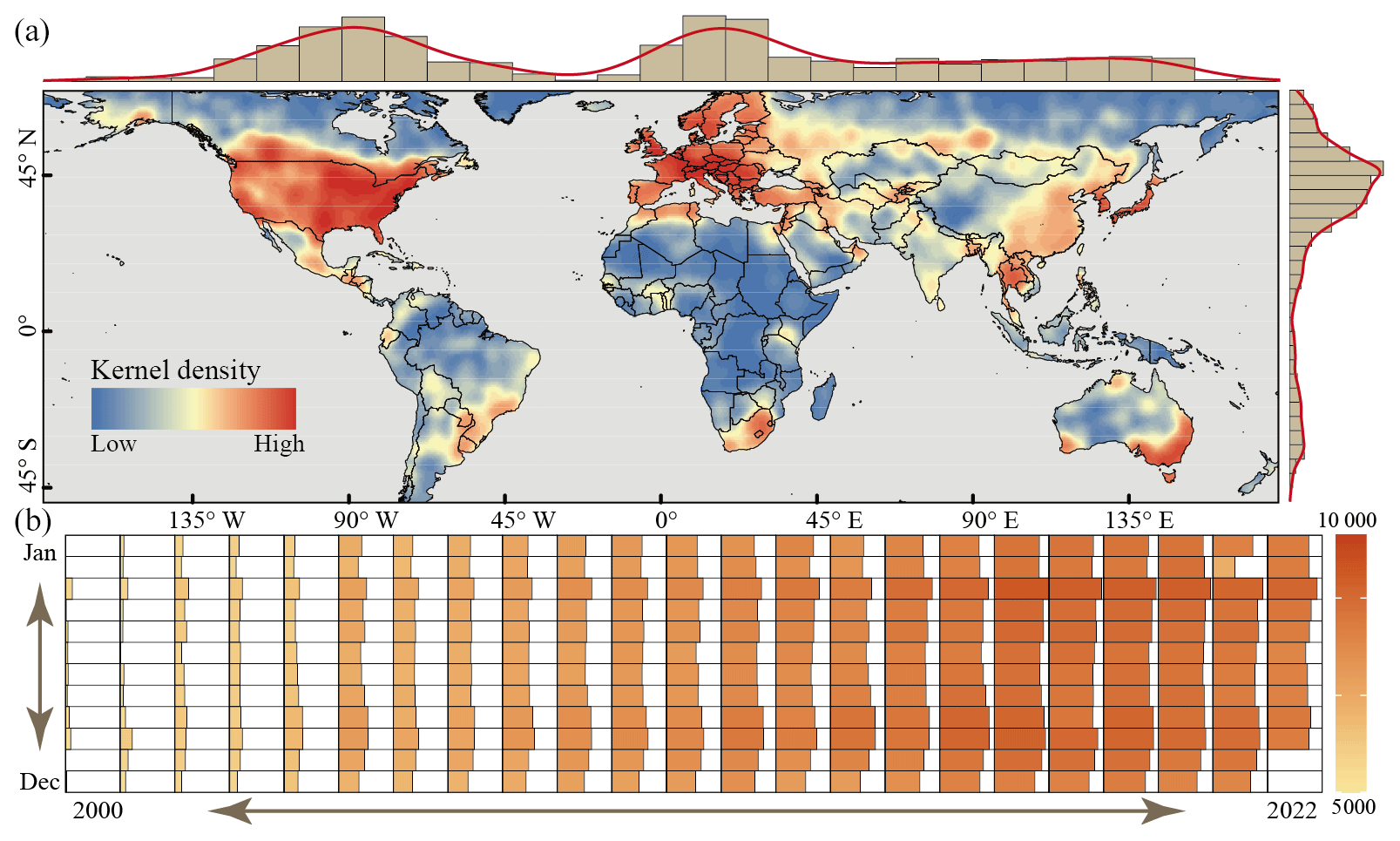
Figure 1 Global monthly meteorological observation samples from 2000 to 2022: (a) kernel density and (b) quantitative statistics.

2.2 Covariate data

We selected seven key covariates in our analysis, specifically LST (land surface temperature), NTL (nighttime lights), LULC (land use–land cover), kNDVI (kernel normalized difference vegetation index), DEM (digital elevation model), month, and LAT (latitude). The selection of these covariates was guided by two fundamental principles. Firstly, we drew from existing research studies to ascertain that the chosen covariates would possess a direct impact on the UTCI or wield significant influence over the meteorological variables employed in UTCI calculations (Fahad et al., 2021; Pappenberger et al., 2015; Wang et al., 2020; Peng et al., 2020b). This ensured the relevance of these covariates to our analysis. Secondly, we took care to select covariates that were openly accessible and obtainable without cost and that originate from data sources with extensive global coverage. This step was essential to guarantee the broad applicability of our analysis, encompassing diverse regions across the world. Here are the details of our data sources and the rationale behind their selection.

LST. We acquired daytime LST data from MOD11A2 (Moderate Resolution Imaging Spectroradiometer) (https://lpdaac.usgs.gov, last access: 16 September 2023). These data are accessible at a spatial resolution of 1 km and compile average values over an 8 d interval from corresponding MOD11A1 LST pixels.

NTL. NTL is indicative of human activities and urbanization. We utilized NPP-VIIRS-like NTL data, available at a spatial resolution of 500 m. This dataset effectively combines data from two NTL sources (DMSP-OLS and NPP-VIIRS), extending the temporal range of NTL observations (Chen et al., 2021). In response to the potential degradation of NTL data (Bai et al., 2023), a series of pre-processing steps in the production of NPP-VIIRS-like NTL data and the proposed cross-sensor calibration can be a great help.

LULC. We sourced LULC data from MODIS_IGBP Land Cover Dataset, which offers a spatial resolution of 500 m. This dataset results from supervised classification using MODIS Terra and Aqua reflectance data and categorizes land cover into 17 distinct types (Loveland et al., 2000). It provides annual data from 2001 to 2021. In instances that we required LULC data for the years 2000 and 2022, we substituted them with data from 2001 and 2021, respectively.

kNDVI. This novel vegetation index is calculated based on NDVI, offering advantages in terms of resistance to saturation, bias, and noise (Camps-Valls et al., 2021). It also demonstrates greater stability at various spatial and temporal scales. We computed kNDVI using MOD13A2 (https://lpdaac.usgs.gov, last access: 16 September 2023).

DEM. We employed the Multi-Error-Removed Improved-Terrain DEM (MERIT DEM) as the DEM data source. This global DEM boasts high accuracy and possesses a resolution of 3 arcsec (approximately 90 m at the Equator) (Hirt, 2018). The MERIT DEM is generated by mitigating major error components in existing DEMs, including the NASA SRTM3 DEM and JAXA AW3D DEM.

Our pre-processing of the aforementioned covariate data involved several steps, including splicing, cropping, resampling, and monthly data synthesis. These steps were undertaken to achieve uniformity in terms of spatial extent, projection, and spatial resolution across all covariates. The covariate data were obtained via the Google Earth Engine (GEE), and resampling techniques were employed to harmonize the spatial resolution of all covariates. Specifically, we adopted the mean resampling method for covariates with continuous values and the nearest-neighbor assignment method for categorical covariates. This ensured that all covariates had consistent spatial resolution. Furthermore, we categorized the seven covariates into two groups based on their characteristics and data availability. One group is dynamically evolving covariates, such as LST and kNDVI, that exert a significant influence on the monthly mean of the UTCI. Therefore, we calculated their monthly mean values. The other group is statically evolving covariates, like latitude, month, and DEM, that impose inherent constraints on the monthly mean of the UTCI. Considering temporal and spatial constraints inherent to raw covariate data availability, and to guarantee temporal and spatial consistency across all covariate data, we ultimately derived monthly covariate data spanning March 2000 to October 2022 within the global latitude range of 50° S to 70° N.

2.3 Existing UTCI datasets

We compared GloUTCI-M with two pre-existing UTCI datasets, namely ERA5-HEAT and HiTiSEA, with the focus on the accuracy of all three datasets. ERA5-HEAT is a worldwide historical dataset encompassing bioclimatic variables, inclusive of the UTCI (Di Napoli et al., 2021). The computation of ERA5-HEAT relies upon ERA5 reanalysis datasets, incorporating meteorological variables such as air temperature, humidity, and wind speed. ERA5-HEAT boasts a spatial granularity of approximately 28 km (0.25°) and a temporal resolution extending up to 1 h. It is freely accessible via the Copernicus Climate Data Store (https://cds.climate.copernicus.eu, last access: 16 September 2023). The HiTiSEA is a gridded product featuring a spatial resolution of 0.1° and contains the daily UTCI spanning 3 January 1981 to 31 December 2019 for the East and South Asian regions (Yan et al., 2021).

3 Methodology

The production process of GloUTCI-M encompasses various key steps, such as the calculation of the UTCI for meteorological samples, the acquisition of covariate data, and the identification of the optimal machine learning model (Fig. 2). We initiated it by utilizing observational data to compute the daily UTCI for the meteorological samples. Subsequently, we synthesized the monthly UTCI based on the availability of daily UTCI data. Following this, we employed three distinct machine learning models to establish the relationship between the monthly UTCI and the covariates. Finally, we validated the accuracy of the training results generated by the machine learning models. Upon completion of this validation process, we selected the optimal machine learning model to produce GloUTCI-M using the covariate raster data. Additionally, leveraging GloUTCI-M, we employed spatiotemporal analysis models, including mutation point analysis and trend analysis, to identify the spatial distribution and temporal fluctuations of the global UTCI.

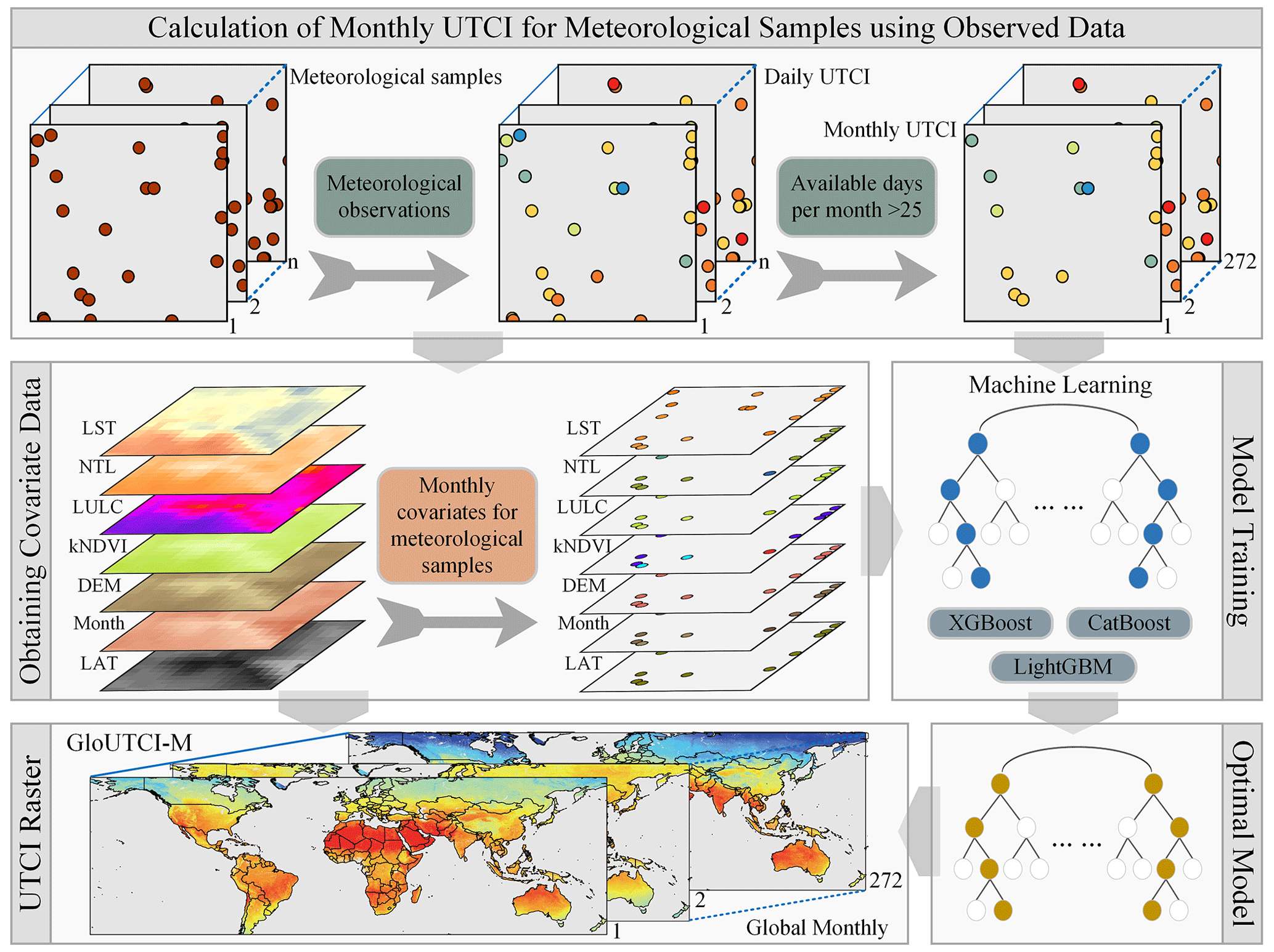
Figure 2 Production process of the GloUTCI-M.

3.1 Calculation of Universal Thermal Climate Index

The deviation between the UTCI and temperature hinges on meteorological variables such as air temperature, mean radiant temperature, wind speed, and water vapor pressure, which can be expressed by the following formula (Bröde et al., 2012):

$$\begin{array}{}\text{(1)}& \text{UTCI}=T_{\mathrm{a}}+\text{Offset}\left(T_{\mathrm{a}}{T}_{\mathrm{mrt}}{V}_{\mathrm{a}}{P}_{\mathrm{a}}\right)=f\left(T_{\mathrm{a}}{T}_{\mathrm{mrt}}{V}_{\mathrm{a}}{P}_{\mathrm{a}}\right),\end{array}$$

where T_a represents air temperature (°C), T_mrt denotes mean radiation temperature (°C), V_a stands for wind speed (m s⁻¹), and P_a corresponds to water vapor pressure (hPa). T_mrt and P_a can be derived from data concerning humidity, solar radiation, and solar altitude angle. Solar radiation data were sourced from ERA5-Land, and solar altitude angles were calculated based on geographical latitude and longitude coordinates. Based on available data from meteorological stations, we selected records captured between 11:00 and 14:00 local time as the daily sample data for UTCI calculations. These daily calculations were then employed to derive the monthly UTCI for each meteorological station, utilizing the BioKlima model (BioKlima ver. 2.6 software) (https://www.igipz.pan.pl, last access: 16 September 2023).

Human comfort levels can be categorized into 10 distinct classes according to UTCI values (Bröde et al., 2012): extreme cold stress ($<-\mathrm{40}$ °C), very strong cold stress (−40 to −27 °C), strong cold stress (−27 to −13 °C), moderate cold stress (−13 to 0 °C), slight cold stress (0–9 °C), no thermal stress (9–26 °C), moderate thermal stress (26–32 °C), strong thermal stress (32–38 °C), very strong thermal stress (38–46 °C), and extreme thermal stress (>46 °C). Therefore, in this study the UTCI below 0 °C implies the presence of cold stress, with temperatures exceeding 26 °C indicating the presence of thermal stress.

3.2 Machine learning models

We applied machine learning models to produce the UTCI dataset because they were more suitable for handling tabular data and could provide a good balance between model performance and computational efficiency. We employed a random division approach to partitioning the monthly UTCI and covariate data, encompassing all meteorological samples worldwide from 2000 to 2022, into a training set (90 %) and a test set for model evaluation (10 %). These subsets served as the basis for training and evaluating three prominent machine learning models: XGBoost, LightGBM, and CatBoost.

3.2.1 XGBoost

Extreme Gradient Boosting (XGBoost) is an integrated machine learning algorithm centered on decision trees, which utilizes a gradient ascent framework for classification and regression tasks (Chen and Guestrin, 2016). XGBoost is particularly effective for tabular data. It excels in capturing complex relationships within the data and provides robust predictions. As a tool for massively parallel boosting trees, it is characterized by its efficiency, flexibility, and portability. XGBoost employs regularization terms in the loss function to control model complexity while approximating the loss function through a second-order Taylor expansion, enhancing model accuracy. It also utilizes techniques like feature subsampling, node splitting, and handling missing values to improve model generalization. XGBoost has wide application in machine learning competitions and various domains, including evapotranspiration estimation, land cover classification, air quality prediction, and aboveground biomass estimation (El Bilali et al., 2023; Katori et al., 2022; Yang et al., 2024). Training for this model was conducted using the Python package xgboost, with hyperparameter tuning performed via grid search, encompassing all feasible combinations of hyperparameters.

3.2.2 LightGBM

Light Gradient Boosting Machine (LightGBM) is a boosting framework that adopts a histogram-based decision tree algorithm to enhance the computational efficiency of Gradient Boosting Decision Trees (GBDT) (Ke et al., 2017). It stands out for its faster training speed, reduced memory consumption, enhanced accuracy, and support for distributed processing. It uses a histogram-based approach for tree construction, which accelerates the training process and makes it well-suited for large datasets. Its ability to handle categorical features efficiently is advantageous for diverse feature set. LightGBM utilizes a leaf-wise tree growth strategy to select the leaf node with the highest gain at each split, enabling faster and deeper tree growth and improving model accuracy. LightGBM has demonstrated its ability to expedite GBDT model training without compromising accuracy and has been applied to various prediction tasks involving spatiotemporal variables (Ahlswede et al., 2023; Aybar et al., 2022). We trained this model using the Python package lightgbm and conducted hyperparameter tuning through a grid search, exploring all potential combinations of hyperparameters.

3.2.3 CatBoost

Categorical Boosting (CatBoost) operates on the symmetric decision tree (oblivious trees) principle, offering few parameters, support for categorical variables, and high accuracy (Prokhorenkova et al., 2018). CatBoost is specifically designed to handle categorical features without the need for extensive pre-processing. It computes statistics on categorical features, such as category frequency, and uses hyperparameters to generate new numerical features. Its categorical boosting approach contributes to its robust performance. The algorithm employs a sort boosting technique to tackle noisy points in the training set, mitigating Gradient Bias and addressing Prediction Shift issues, which reduces overfitting and enhances model accuracy and generalization. CatBoost has wide application in domains like meteorology, hydrology, agriculture, and regression and prediction tasks across various fields (Tasaki et al., 2022; Cravo et al., 2022). We conducted training for this model using the Python package catboost and executed hyperparameter tuning through grid search, systematically exploring all possible combinations of hyperparameters.

3.3 Model evaluation metrics

To assess the suitability of XGBoost, LightGBM, and CatBoost for predicting the UTCI and determine the optimal machine learning model for producing the UTCI dataset, we employed three widely recognized metrics for evaluating predictive models: the mean absolute error (MAE), the root mean square error (RMSE), and the coefficient of determination (R²). Both MAE and RMSE serve as metrics to gauge the overall accuracy of a model by quantifying the magnitude of the error between the predicted values and the observed values. MAE is computed as the average of the absolute differences between the predicted and observed values, while RMSE represents the square root of the average of the squared differences between predicted and observed values. Smaller values for MAE and RMSE indicate a more precise prediction. R² measures the extent to which the model fits the data and ranges between 0 and 1. A value closer to 1 signifies a superior model fit. The calculations for these three indicators are as follows:

$$\begin{array}{}\text{(2)}& {\displaystyle }\mathrm{MAE}={\displaystyle \frac{\mathrm{1}}{n}}\sum _{i=\mathrm{1}}^n\left|P_i-C_i\right|\text{(3)}& {\displaystyle }\mathrm{RMSE}=\sqrt{{\displaystyle \frac{\mathrm{1}}{n}}\sum _{i=\mathrm{1}}^n(P_i-C_i{)}^{\mathrm{2}}}\text{(4)}& {\displaystyle }{R}^{\mathrm{2}}=\mathrm{1}-\sum _{i=\mathrm{1}}^n(C_i-P_i{)}^{\mathrm{2}}/\sum _{i=\mathrm{1}}^n(C_i-\overline{C}{)}^{\mathrm{2}},\end{array}$$

where P_i represents the predicted UTCI, C_i denotes the observed UTCI calculated based on data from the meteorological samples, $\overline{C}$ is the average value of all C_i, and n signifies the number of samples. The test dataset was utilized to compute these evaluation metrics, thereby enabling the assessment of the machine learning model for UTCI prediction capability.

3.4 Spatiotemporal analysis

To comprehensively understand the spatiotemporal distribution of the global UTCI, we employ two distinct analytical methods: the Bayesian model averaging time-series decomposition algorithm (BEAST) to identify the characteristics of the global UTCI from the spatial perspective, and the Theil–Sen median analysis along with the Mann–Kendall (MK) method to understand the changing trend of the global UTCI from the temporal perspective.

BEAST analysis is a Bayesian model averaging algorithm designed for the decomposition of numerical series data (Zhao et al., 2019). Its primary purpose is to identify key characteristics such as mutation points and nonlinear trends within the data. BEAST is advantageous because it enhances the accuracy of detecting mutation points by providing prior and posterior probability distributions for these points. It quantifies the inherent uncertainty associated with mutation detection by assigning quantitative probabilities. BEAST has been widely applied in diverse numerical series data, including financial, public health, economic, and ecological datasets (Mulverhill et al., 2023; Pitarch et al., 2021). To address the issue of potentially differing or conflicting estimation results produced by various models, BEAST employs Bayesian modeling to assess the relative importance of individual models; averages the results from multiple models; and decomposes the observation in the numerical series into three components, i.e., the trend signal, seasonal signal (for the time series), and residual signal, with the trend signal for further mutation points' identification (Zhao et al., 2019).

The trend analysis carried out by the Theil–Sen slope estimation method and the test of significance of the trend using the MK method can reflect the effective trend of each pixel in the time series. This comprehensive method has been widely used in the trend significance test of long-time-series data in many fields such as ecology, meteorology and hydrology (He et al., 2022; Hu et al., 2023). The Theil–Sen slope estimation method is a robust nonparametric statistical technique used for trend calculation. It is insensitive to measurement errors and outlier data and thus is effective in handling missing value noise. This method computes slopes between pairs of data points in the time series and calculates the median of these slopes to determine the overall trend (Zheng et al., 2021).

$$\begin{array}{}\text{(5)}& \mathit{\beta }=\mathrm{median}\left({\displaystyle \frac{X_j-X_i}{j-i}}\right)\forall j>i,\end{array}$$

where X_j and X_i represent observed data points in the time series, and β indicates the overall trend. If β is greater than 0, it suggests an increasing trend, while β less than 0 indicates a decreasing trend.

The MK method is a nonparametric test that does not require the measurements to follow a normal distribution. It is robust against missing values and outliers and is used to test the significance of the time-series trend as a supplement to the Theil–Sen slope estimation method. The test statistic is calculated based on the relationship between data values in the time series X_i (i=1, 2, 3, …, n) (Peng et al., 2023).

$$\begin{array}{}\text{(6)}& {\displaystyle }Z=\left\{\begin{array}{cc}\frac{S}{\sqrt{\mathrm{Var}\left(S\right)}}& (S>\mathrm{0})\\ \mathrm{0}& (S=\mathrm{0})\\ \frac{S+\mathrm{1}}{\sqrt{\mathrm{Var}\left(S\right)}}& (S<\mathrm{0})\end{array}\right.\text{(7)}& {\displaystyle }\mathrm{Var}\left(S\right)={\displaystyle \frac{n(n-\mathrm{1})(\mathrm{2}n+\mathrm{5})}{\mathrm{18}}},\end{array}$$

where Z is the standardized test statistic, S is the relationship between the size of X_i and X_j among all pairs of values (X_j,X_i, j>i) in the time series, and n is the number of data in the time series. When the absolute value of Z exceeds certain critical values (1.65, 1.96, and 2.58), it indicates that the trend is statistically significant at confidence levels of 90 %, 95 %, and 99 %, respectively. The 95 % confidence level is commonly employed in this study.

4 Results

4.1 Model performance

To identify the optimal machine learning model for achieving heightened accuracy in the global monthly UTCI dataset, we employed the test dataset to assess the performance of XGBoost, LightGBM, and CatBoost. Our evaluation process consisted of two key steps. Firstly, we juxtaposed the predicted UTCI generated by each model against the observed UTCI from meteorological station samples and then calculated accuracy metrics such as MAE, RMSE, and R² (Fig. 3). Secondly, we computed the mean of the absolute residuals (MAR) between the predicted UTCI and the observed UTCI at globally available meteorological stations (Fig. 4). This allowed us to discern global variations in the performance of the three models.

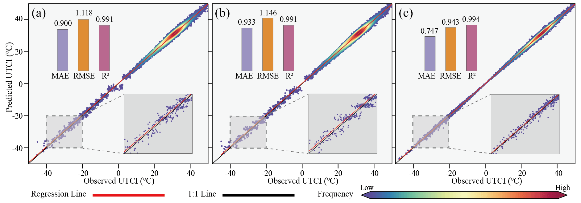
Figure 3 Comparison of the predicted UTCI derived from machine learning models with the observed UTCI obtained from meteorological station samples: (a) XGBoost, (b) LightGBM, and (c) CatBoost.

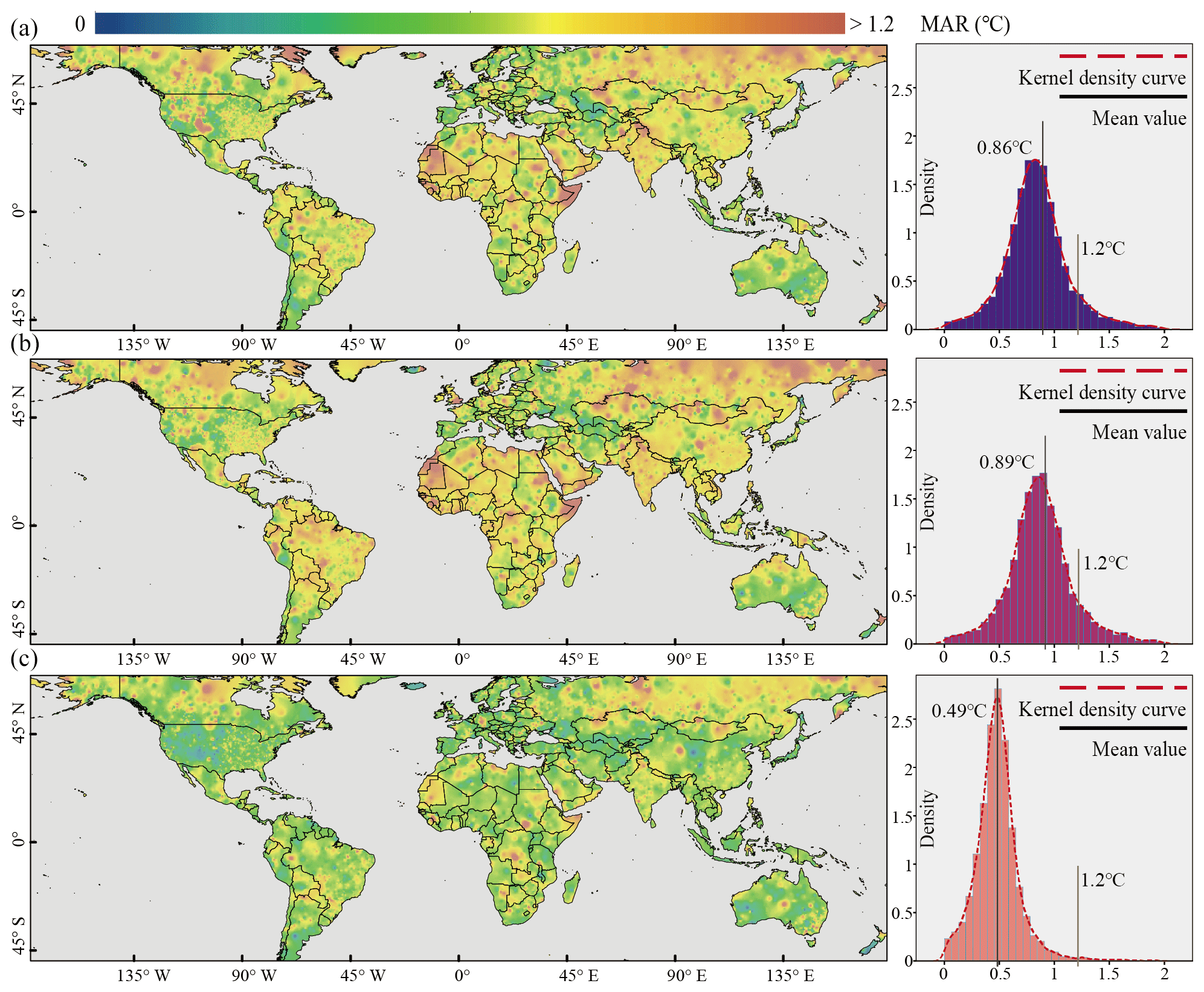
Figure 4 Spatially interpolated distribution and statistics of MAR between the predicted UTCI and the observed UTCI for global meteorological stations: (a) XGBoost, (b) LightGBM, and (c) CatBoost.

The concordance between the predicted UTCI and the observed UTCI was notably strong for all three models, as evidenced by data points predominantly clustering around the 1:1 line. The positional deviation between the regression line and the 1:1 line for lower UTCI values signifies varying degrees of overestimation in the UTCI predictions of the three models. Notably, LightGBM exhibited a relatively larger positional deviation between the regression line and the 1:1 line (Fig. 3b), followed by XGBoost (Fig. 3a), with CatBoost demonstrating the smallest deviation (Fig. 3c). Regarding MAE, both XGBoost and LightGBM exhibited values close to 0.9 °C, with a slightly smaller MAE for XGBoost. In stark contrast, CatBoost boasted a substantially lower MAE of 0.747 °C, clearly surpassing the performance of XGBoost and LightGBM. The RMSE among the three models exhibited significant disparities but maintain the same order as the MAEs, with CatBoost outperforming XGBoost and LightGBM. It was noteworthy that both XGBoost and LightGBM surpassed an RMSE of 1.1 °C, whereas CatBoost excelled with an RMSE of under 1 °C. Furthermore, all three models exhibited high values for the R². XGBoost and LightGBM closely approximated with an R² of 0.991, while CatBoost excelled with the highest R², reaching 0.994. Consequently, the performance of CatBoost surpassed that of XGBoost and LightGBM in terms of MAE, RMSE, and R².

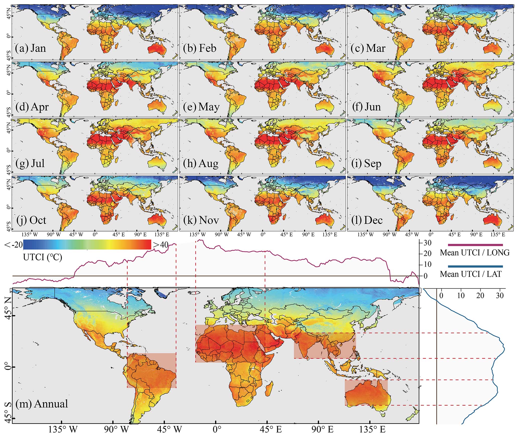
Figure 5 Global distribution of the monthly and annual UTCI in 2021.

Utilizing the MAR between the predicted UTCI and the observed UTCI from all available global meteorological stations (9083 stations), we employed spatial interpolation to discern global performance disparities among XGBoost (Fig. 4a), LightGBM (Fig. 4b), and CatBoost (Fig. 4c). The global distribution of the MAR for the three models exhibited a consistent pattern. Regions densely populated with meteorological stations, such as the United States and Europe, displayed smaller MAR, while regions with fewer meteorological stations, such as Africa and northern Asia, manifested larger MAR. Notably, the MARs of XGBoost and LightGBM exhibited substantial spatial enlargement compared to that of CatBoost. Specifically, MARs exceeding 1.2 °C extended over significant expanses, including western Africa, the Siberian region of Russia, and northern Canada. In these regions, CatBoost's MAR remained relatively modest, with only sporadic areas where MAR exceeded 1.2 °C. In other global regions, CatBoost consistently maintained a significantly lower MAR in comparison to XGBoost and LightGBM. The mean MAR for XGBoost and LightGBM was similar, standing at 0.86 and 0.89 °C, respectively, but both were notably higher than CatBoost's mean MAR of 0.49 °C. Additionally, the count of stations registering MAR exceeding 1.2 °C reached 956 for XGBoost and 1102 for LightGBM, constituting more than 10 % of the meteorological stations (10.5 % and 12.1 %, respectively). In contrast, CatBoost displayed only 96 meteorological stations with MAR exceeding 1.2 °C, accounting for a mere 1.1 % of the total meteorological stations. Consequently, CatBoost also demonstrated superior performance over XGBoost and LightGBM concerning the spatial and numerical distribution of MAR.

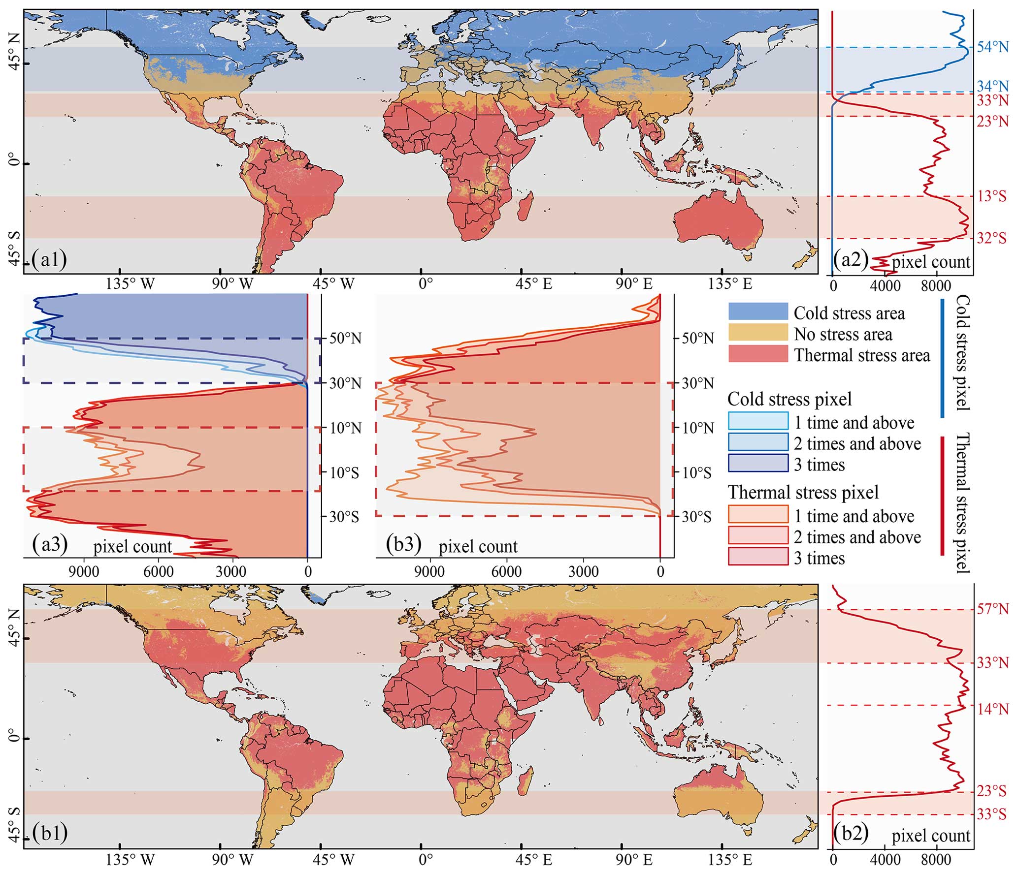
Figure 6 Global distribution and statistics of cold and thermal stress areas globally in 2021: (a1) winter months, (b1) summer months, (a2) latitudinal series of winter months, (b2) latitudinal series of summer months, (a3) type of pixel on the latitude series of winter months, and (b3) type of pixel on the latitude series of summer months.

4.2 Spatial distribution of the UTCI

Based on the assessment of the three models, CatBoost emerged as the optimal choice for estimating the global monthly UTCI. Consequently, we employed CatBoost to produce the global monthly 1 km Universal Thermal Climate Index dataset spanning 2000 to 2022, known as GloUTCI-M. Utilizing the monthly UTCI data for 2021, along with its annual counterpart, we conducted an analysis to discern the spatial distribution pattern of the global UTCI (Fig. 5). Moreover, we extracted cold stress and thermal stress pixels for each winter month (referring to the nomenclature of the Northern Hemisphere, i.e., December, January, and February) and each summer month (referring to the nomenclature of the Northern Hemisphere, i.e., June, July, and August) in 2021, respectively. This enabled us to delineate the worldwide distribution of cold and thermal stress areas (Fig. 6).

The distribution pattern of the global monthly UTCI revealed notable differences between the Northern Hemisphere and the Southern Hemisphere, as well as seasonal variations. In the Northern Hemisphere, there were prominent latitudinal variations, with the UTCI generally decreasing from the Equator towards higher latitudes across all months. The trend of the UTCI in the Southern Hemisphere exhibited less significant changes with increasing latitude. Furthermore, the disparity in the UTCI between the two hemispheres became more pronounced during the winter months, particularly in terms of latitude-related differences. Conversely, this difference diminished during the summer months. The global distribution of the monthly UTCI also exhibited reasonable variations in accordance with the changing seasons. During the summer months (Fig. 5f–h), there was a substantial concentration of high UTCI pixels (>40 °C), while low UTCI pixels ($<-\mathrm{20}$ °C) were less prevalent in both the Northern Hemisphere and Southern Hemisphere. In contrast, the Northern Hemisphere experienced a notable abundance of low UTCI pixels in the winter months (Fig. 5a, b, and l). Furthermore, we computed the mean UTCI at each longitude and latitude based on annual UTCI data and represented them in a line plot (Fig. 5m). This plot highlighted two regions with the relatively high UTCI in northern South America and northern Africa. In the latitudinal perspective, regions with the relatively high UTCI were also evident in southern Asia and Australia.

The global distribution of cold stress areas (UTCI <0 °C) and thermal stress areas (UTCI >26 °C) during the winter months, as determined by the mean UTCI exhibited significant latitudinal heterogeneity (Fig. 6a1). The concentration of cold stress areas was particularly notable in the northern regions of North America and the Asian–European continent. Conversely, no-stress areas encompassed regions such as the United States, the Mediterranean, and China. Thermal stress areas were widely dispersed, encompassing the majority of the Southern Hemisphere and the region between the Equator and the Tropic of Cancer. By employing BEAST analysis, we identified mutation points in the quantity of cold and thermal stress pixels along the latitudinal sequence (Fig. 6a2). Notably, the spatial range from 54 to 34° N experienced a substantial reduction in cold stress pixels, while thermal stress pixels showed a rapid increase between 33 and 23° N, with another increase between 13 and 32° S. Furthermore, the number of occurrences of cold and thermal stress pixels at each latitude during the three winter months was examined separately (Fig. 6a3). It was observed that cold stress pixels in the region above 50° N remained relatively stable throughout the three winter months, whereas there were significant monthly fluctuations in the region between 30 and 50° N. Conversely, the thermal stress pixel displayed significant monthly fluctuations in the region from 15° S to 10° N.

During the summer months, the global thermal stress area, exhibited widespread distribution, while the cold stress area was more sporadic (Fig. 6b1). The majority of the regions around the Equator fell within the thermal stress area. Conversely, other regions (such as the northern part of North America; most of Europe; and the southern part of South America, Africa, and Australia) were characterized by high concentration of no-stress areas. Given the limited presence of cold stress areas, we focused on plotting the number of thermal stress pixel occurrences along the latitudinal series and employed BEAST analysis to pinpoint mutation points (Fig. 6b2). The interval from 57 to 33° N experienced a significant increase in the number of thermal stress pixel, and this number remained consistently high within the 33° N–23° S interval (with fluctuations within the 14° N–23° S interval). However, a sharp decrease in the number of thermal stress pixels was observed in the 23–33° S interval. Furthermore, there were substantial monthly fluctuations in the number of thermal stress pixel occurrences across latitudes during the three summer months (Fig. 6b3). This phenomenon was particularly pronounced in the 30° N–30° S interval, where a large number of pixels experienced thermal stress in only one or two of the summer months.

4.3 Temporal trends of the UTCI

Utilizing GloUTCI-M, we examined the time-series evolution of the global UTCI. Initially, we compiled the monthly global UTCI from 2000 to 2022, along with the mean annual UTCI from 2001 to 2021. Subsequently, we constructed individual scatter plots to gain insight into the fluctuations in the global UTCI (Fig. 7). Furthermore, we extracted the mean annual UTCI for global pixels and employed the Theil–Sen slope estimation method and the MK method to identify the trend of the global UTCI (Fig. 8).

Between the years from 2000 to 2022, there was a noteworthy increase in the mean global UTCI during the summer months (June–September) with statistical significance (p<0.05). In contrast, the trend in the mean global UTCI during winter was mostly non-significant (p>0.05). Additionally, the trend in the mean annual global UTCI demonstrated a substantial elevation (R²=0.66, p<0.05) (Fig. 7m). To gain a deeper understanding of how each month's UTCI contributed to or suppressed the mean annual global UTCI from 2001 to 2021, we produced waterfall plots (Fig. 7n). This plot allowed us to discern the positive or negative impact of each month's UTCI by comparing the difference between the annual UTCI and the UTCI for that specific month. The mean annual global UTCI for the period 2001–2021 was 17.24 °C. Out of the 12 months, 7 months (April–October) made a positive contribution towards achieving the mean annual global UTCI. Among these, July held the most substantial contribution (+9.86 °C), followed by August (+8.97 °C) and June (+8.92 °C). Conversely, the remaining 5 months (January–March, November, and December) fell below the mean annual global UTCI. Among these, January exerted the most significant inhibitory effect (−11.96 °C), while December and February also displayed notable inhibitory effects (−11.05 and −9.33 °C, respectively).

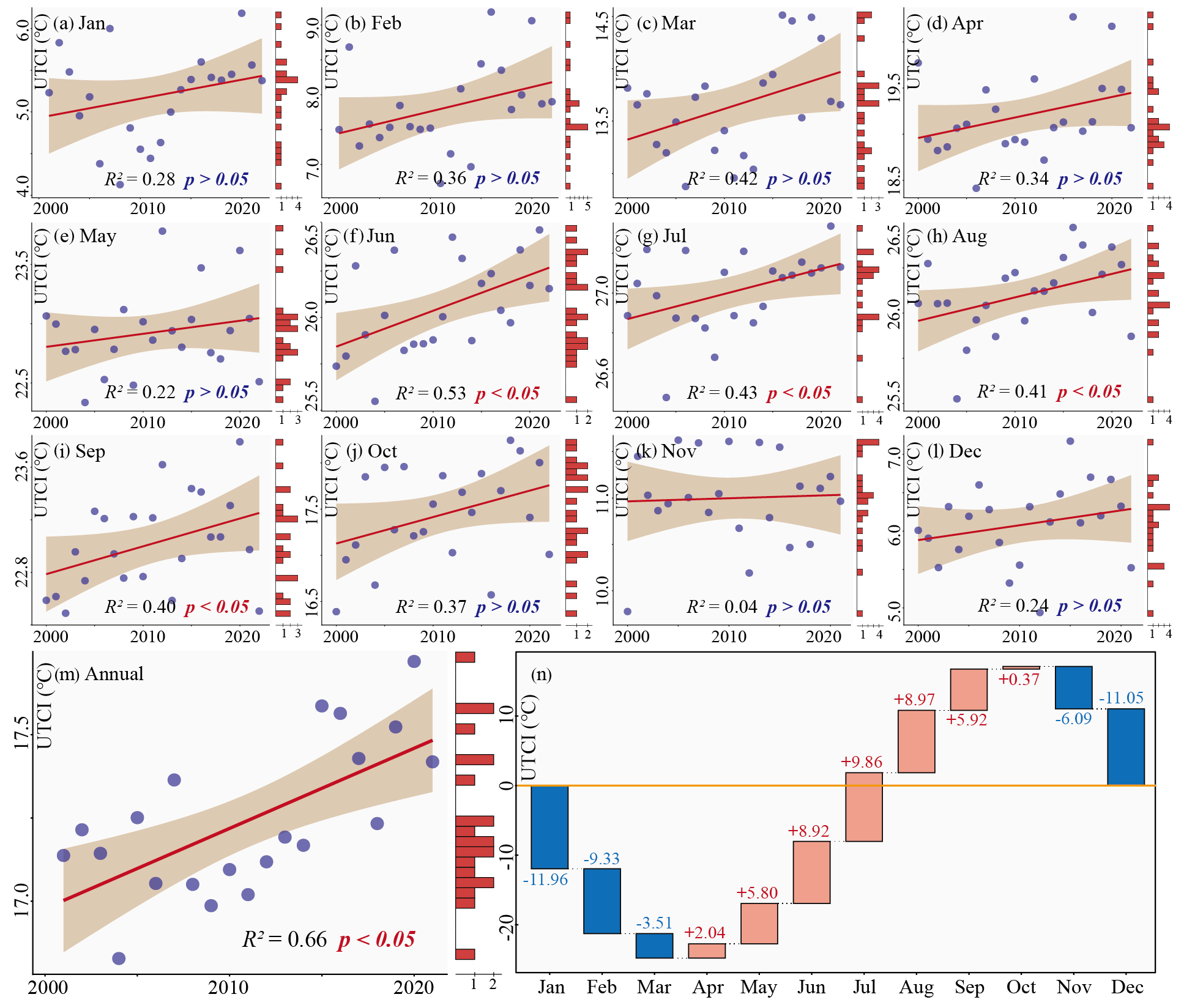
Figure 7 Global monthly and annual UTCI changes from 2000 to 2022: (a–l) monthly UTCI changes, (m) annual UTCI changes, and (n) difference between each monthly UTCI and the annual UTCI.

The annual UTCI trends for global pixels were predominantly characterized by a significantly increasing trend and a non-significant trend, with few pixels exhibiting significantly decreasing trend (Fig. 8a). Regions displaying an increasing UTCI trend included the western United States (Fig. 8b1), the eastern part of Brazil (Fig. 8b2), western Europe (Fig. 8b3), Southeast Asia (Fig. 8b4), and the eastern part of China (Fig. 8b5). Regions with a decreasing UTCI trend were primarily situated in southern Mexico (Fig. 8c1), northern South America (Fig. 8c2), central Africa (Fig. 8c3), western India (Fig. 8c4), and southwestern China (Fig. 8c5). Additionally, we separately counted the top 10 countries with the highest pixel number of UTCI trends showing increasing or decreasing patterns. Regions such as Russia in Asia and Europe, Brazil in South America, and Libya in Africa had over 1 000 000 pixels exhibiting an increasing UTCI trend, which served as hotspots driving the increase in the mean annual global UTCI (Fig. 8d1). Both China and India had more than 500 000 pixels displaying a decreasing UTCI trend, playing a significant role in mitigating the elevation of the mean annual global UTCI (Fig. 8d2).

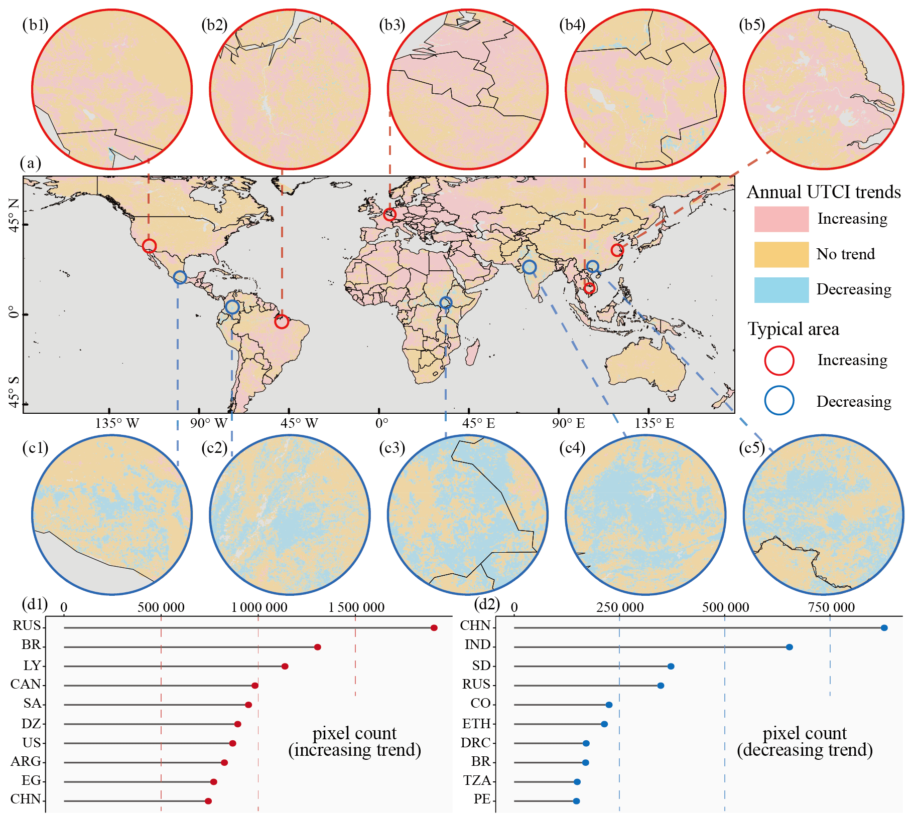
Figure 8 Significant trends in the annual UTCI for global pixels: (a) spatial distribution, (b1–b5) typical areas with increasing trend in the annual UTCI, (c1–c5) typical areas with decreasing trend in the annual UTCI, (d1) top 10 countries with the highest number of pixels showing an increasing trend in the annual UTCI, and (d2) top 10 countries with the highest number of pixels showing a decreasing trend in the annual UTCI.

5 Discussion

5.1 Comparison with existing UTCI dataset

Given the availability of existing UTCI datasets, we undertook a comparative analysis of the spatial distributions of ERA5-HEAT, HiTiSEA, and GloUTCI-M across various scales, including the intercontinental, city cluster, and city scales. We extracted UTCI data from the ERA5-HEAT between 11:00 and 14:00 local time to calculate the monthly UTCI for the year 2019. Simultaneously, we extracted the maximum daily UTCI from the HiTiSEA to derive the monthly UTCI for the same year. Moreover, we compared the data quality of the three types of datasets by plotting Taylor diagrams and using RMSE and R². Specifically, using the year 2019 as a case study, we selected meteorological stations situated in East and South Asia as representative samples. We then calculated the disparities between the monthly UTCI obtained from the three datasets and those derived from meteorological observation data for summer (June, July, and August), winter (December, January, and February), and all 12 months throughout the year.

ERA5-HEAT, HiTiSEA, and GloUTCI-M manifested analogous UTCI spatial pattern at the intercontinental scale (Fig. 9). Nevertheless, at the city cluster and city scales, GloUTCI-M exhibited marked advantages. Specifically, GloUTCI-M excelled in delineating intricate variations in the UTCI within urban areas. Furthermore, we conducted a comprehensive assessment by comparing the disparities between these three datasets and the observed UTCI collected from meteorological stations. This evaluation, represented by Taylor diagrams, elucidated the disparities in accuracy among the trio. When examining winter and year-round samples, all three datasets demonstrated a robust correlation with the observed UTCI. Notably, GloUTCI-M yielded the smallest RMSE, with HiTiSEA and ERA5-HEAT following closely (Fig. 9d and f). In the case of summer month samples, the R² between GloUTCI-M and the observed UTCI consistently exceeded 0.95, whereas the R² values between ERA5-HEAT and HiTiSEA and the observed UTCI lingered below 0.8. Furthermore, the RMSE between ERA5-HEAT and HiTiSEA in comparison to the observed UTCI significantly surpassed that of GloUTCI-M (Fig. 9e). Hence, in contrast to ERA5-HEAT and HiTiSEA, GloUTCI-M excelled in portraying UTCI distribution at smaller spatial scales with superior data accuracy, marked by diminished RMSE.

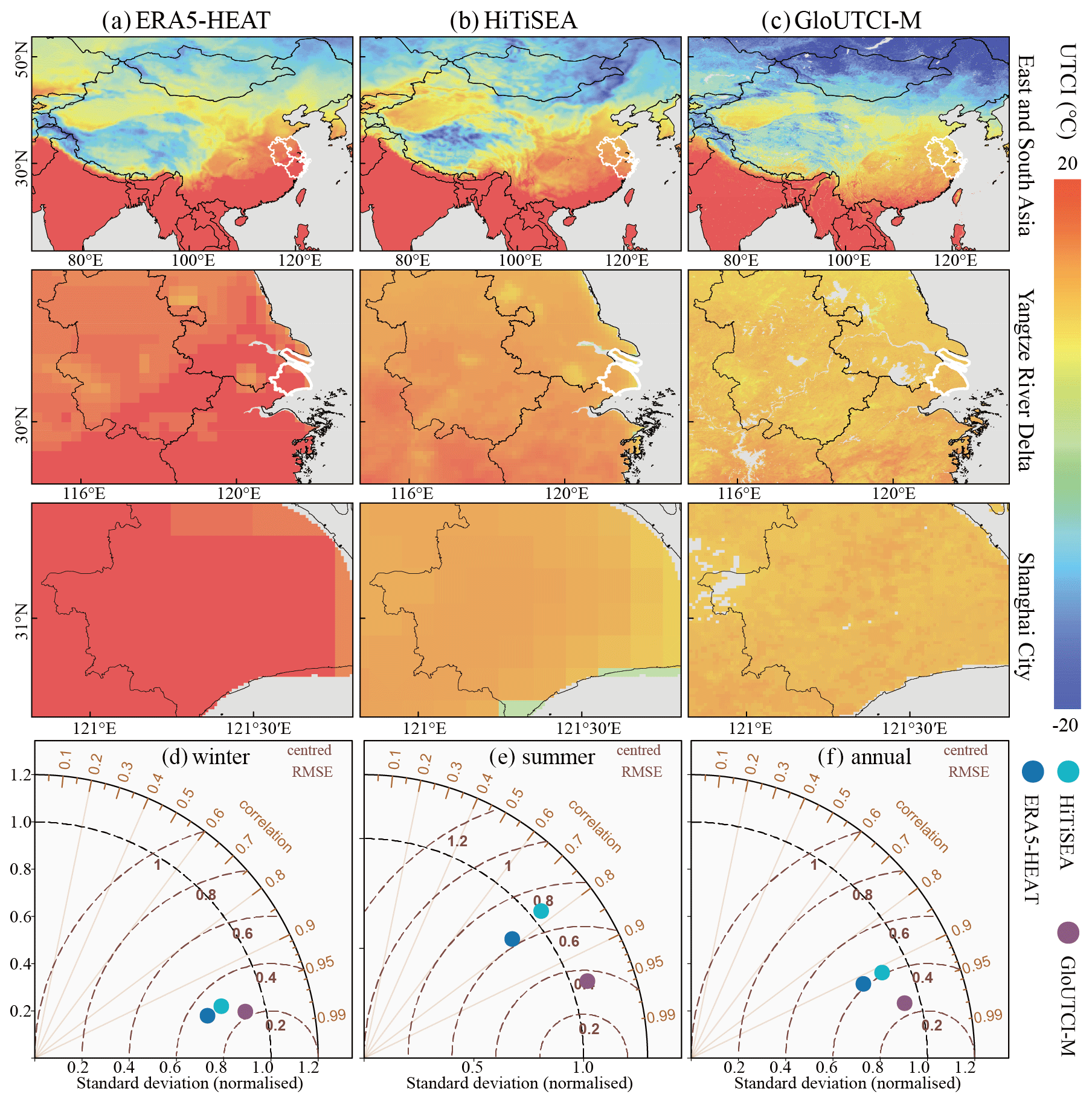
Figure 9 Comparison of spatial distribution and data accuracy among ERA5-HEAT, HiTiSEA and GloUTCI-M: (a) ERA5-HEAT at different spatial scales, (b) HiTiSEA at different spatial scales, (c) GloUTCI-M at different spatial scales, (d) comparison of three UTCI datasets with the observed UTCI for winter months, (e) comparison of three UTCI datasets with the observed UTCI for summer months, and (f) comparison of three UTCI datasets with the annual observed UTCI.

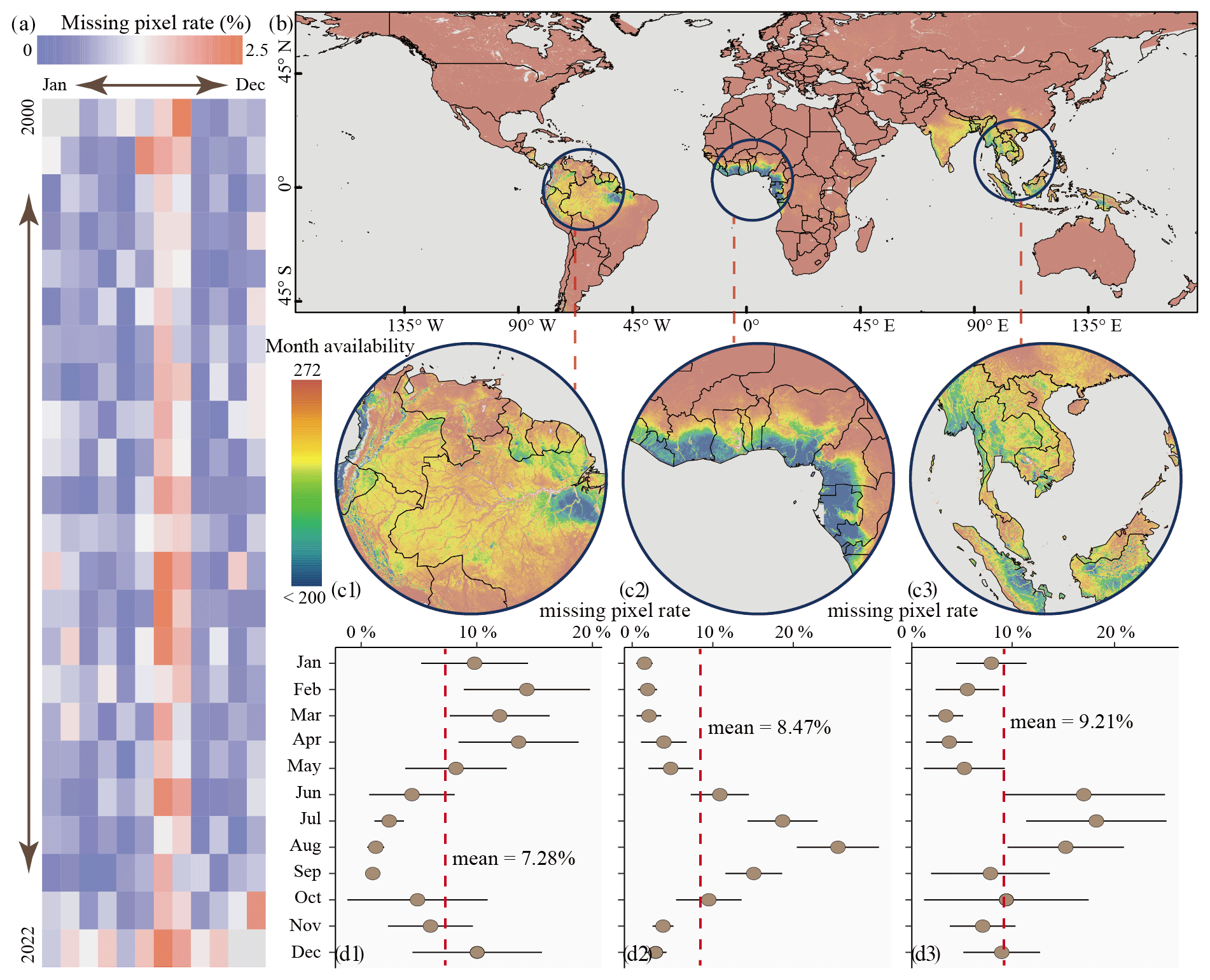
Figure 10 Month availability of pixels for GloUTCI-M data: (a) global missing pixel rate for each month, (b) spatial distribution of month availability, (c1–c3) areas of densely missing pixels for monthly data, and (d1–d3) missing pixel rate by month for areas of densely missing pixels.

5.2 Global distribution of month availability

The existence of voids in the raster dataset of covariates, attributed to factors such as cloud cover and spatiotemporal discontinuities, resulted in lacking spatiotemporal seamlessness of the GloUTCI-M product. To elucidate the global spatiotemporal availability of GloUTCI-M, we conducted a comprehensive assessment of pixel availability across 272 months. Spanning from March 2000 to October 2022, GloUTCI-M had a maximum missing pixel rate of 2.5 % for the monthly UTCI data. However, it is noteworthy that the majority of months within this time frame exhibited a missing pixel rate of less than 1 %. Furthermore, when scrutinizing individual months, July and August consistently emerged with higher rates of missing pixel across all years than other months (Fig. 10a).

GloUTCI-M boasted robust month availability across the majority of global regions (Fig. 10b). Nevertheless, there were three regions characterized by densely low month availability. These regions included the northern part of South America (Fig. 10c1), the western coast of Africa (Fig. 10c2), and Southeast Asia (Fig. 10c3). Examining the month-averaged missing pixel rates for these regions, we could observe values below 10 %. Southeast Asia reported the highest missing pixel rate at 9.21 %, followed by the west coast of Africa at 8.47 %, while northern South America recorded relatively low rates at 7.28 %. Notably, these regions exhibited varying trends in missing pixel rates by month. For northern South America, the period from January through May and December showcased above-average missing pixel rates, notably exceeding 10 % from February through April (Fig. 10d1). Conversely, the west coast of Africa experienced a concentration of missing pixels from June to September, with August peaking at more than 20 % (Fig. 10d2). Southeast Asia exhibited heightened missing pixel rates from June through August, all surpassing 15 % (Fig. 10d3).

5.3 Limitations and future works

The production of GloUTCI-M is intrinsically linked to the quality of the covariate data. Consequently, the existence of missing pixels within these covariates would result in varying degrees of monthly UTCI data missing for global pixels of GloUTCI-M. To enhance both the accuracy and data availability of the GloUTCI-M, a viable avenue is to identify and utilize spatiotemporally seamless remote sensing data for the covariates. Several covariates, such as LST, LULC, and kNDVI, utilized in the GloUTCI-M production process were drawn from the MODIS data. Consequently, GloUTCI-M exclusively comprises global monthly UTCI data spanning March 2000 to October 2022, as there is no access to MODIS data before 2000. A promising strategy for extending the temporal range of the global monthly UTCI dataset involves leveraging available covariate data from different time periods to produce UTCI datasets corresponding to those specific time periods. Subsequently, by fusing these datasets, the expansion of the temporal coverage of the global monthly UTCI dataset can be realized.

6 Data availability

The GloUTCI-M comprises global monthly UTCI data at a spatial resolution of 1 km, spanning March 2000 to October 2022. This dataset is openly accessible in GeoTIFF format via Zenodo: https://doi.org/10.5281/zenodo.8310513 (Yang et al., 2023). The dataset is expressed in degrees Celsius (°C) and is stored as an integer type (Int16). To utilize it appropriately, one must divide the values by 100.

7 Conclusion

To address the existing gaps in UTCI data availability and enhance the applicability of the UTCI in various domains, we have produced a global monthly UTCI dataset, i.e., GloUTCI-M, which boasts global coverage, a long time series spanning March 2000 to October 2022, and a high spatial resolution of 1 km. GloUTCI-M is the result of amalgamating multiple data sources (including LST, NTL, LULC, kNDVI, and DEM) and employing an optimized machine learning model of CatBoost. Our analysis of the spatial and temporal evolution of the global UTCI, based on GloUTCI-M, revealed disparities between the Northern Hemisphere and the Southern Hemisphere, as well as seasonal fluctuations. Significant latitudinal variations were apparent in the distribution of global cold and thermal stress areas. During the summer months (June–September), the global mean UTCI experienced a notable increase, with an even more pronounced elevation observed in the trend of the global mean annual UTCI. This trend, at the pixel level, was predominantly characterized by an increasing trend, with few pixels displaying a decreasing trend. In the global UTCI trend, countries like Russia and Brazil emerged as key contributors to the rising global mean annual UTCI, while countries such as China and India exerted a greater influence in mitigating this rise. In addition, when compared to existing UTCI datasets such as ERA5-HEAT and HiTiSEA, GloUTCI-M excelled in portraying UTCI distributions at fine spatial scales and offering superior data accuracy. It is anticipated that the GloUTCI-M will serve as a valuable resource, providing comprehensive and accurate information to support research and policymaking across various domains, including meteorological science, health management, urban planning, and agriculture. Its utility extends to enhancing human comfort, reducing weather-related health risks, and facilitating better adaptation to the challenges posed by climate change.