the Creative Commons Attribution 4.0 License.
the Creative Commons Attribution 4.0 License.
 | 07 Mar 2023
National CO2 budgets (2015–2020) inferred from atmospheric CO2 observations in support of the global stocktake
Brendan Byrne
David F. Baker
Sourish Basu
Michael Bertolacci
Kevin W. Bowman
Dustin Carroll
Abhishek Chatterjee
Frédéric Chevallier
Philippe Ciais
Noel Cressie
David Crisp
Sean Crowell
Feng Deng
Nicholas M. Deutscher
Manvendra K. Dubey
Omaira E. García
David W. T. Griffith
Benedikt Herkommer
Andrew R. Jacobson
Rajesh Janardanan
Sujong Jeong
Matthew S. Johnson
Dylan B. A. Jones
Rigel Kivi
Junjie Liu
Zhiqiang Liu
Shamil Maksyutov
John B. Miller
Scot M. Miller
Isamu Morino
Justus Notholt
Tomohiro Oda
Christopher W. O'Dell
Young-Suk Oh
Hirofumi Ohyama
Prabir K. Patra
Hélène Peiro
Christof Petri
Sajeev Philip
David F. Pollard
Benjamin Poulter
Marine Remaud
Andrew Schuh
Mahesh K. Sha
Kei Shiomi
Kimberly Strong
Colm Sweeney
Hanqin Tian
Voltaire A. Velazco
Mihalis Vrekoussis
Thorsten Warneke
John R. Worden
Debra Wunch
Yuanzhi Yao
Jeongmin Yun
Andrew Zammit-Mangion
Ning Zeng
Accurate accounting of emissions and removals of CO2 is critical for the planning and verification of emission reduction targets in support of the Paris Agreement. Here, we present a pilot dataset of country-specific net carbon exchange (NCE; fossil plus terrestrial ecosystem fluxes) and terrestrial carbon stock changes aimed at informing countries' carbon budgets. These estimates are based on “top-down” NCE outputs from the v10 Orbiting Carbon Observatory (OCO-2) modeling intercomparison project (MIP), wherein an ensemble of inverse modeling groups conducted standardized experiments assimilating OCO-2 column-averaged dry-air mole fraction () retrievals (ACOS v10), in situ CO2 measurements or combinations of these data. The v10 OCO-2 MIP NCE estimates are combined with “bottom-up” estimates of fossil fuel emissions and lateral carbon fluxes to estimate changes in terrestrial carbon stocks, which are impacted by anthropogenic and natural drivers. These flux and stock change estimates are reported annually (2015–2020) as both a global 1∘ × 1∘ gridded dataset and a country-level dataset and are available for download from the Committee on Earth Observation Satellites' (CEOS) website: https://doi.org/10.48588/npf6-sw92 (Byrne et al., 2022). Across the v10 OCO-2 MIP experiments, we obtain increases in the ensemble median terrestrial carbon stocks of 3.29–4.58 Pg CO2 yr−1 (0.90–1.25 Pg C yr−1). This is a result of broad increases in terrestrial carbon stocks across the northern extratropics, while the tropics generally have stock losses but with considerable regional variability and differences between v10 OCO-2 MIP experiments. We discuss the state of the science for tracking emissions and removals using top-down methods, including current limitations and future developments towards top-down monitoring and verification systems.
- Article
(6581 KB) - Full-text XML
-
Supplement
(13878 KB) - BibTeX
- EndNote


© 2023. California Institute of Technology. Government sponsorship acknowledged.
To reduce the risks and impacts of climate change, the Paris Agreement aims to limit the global average temperature increase to well below 2 ∘C above pre-industrial levels and to pursue efforts to limit these increases to less than 1.5 ∘C. To this end, each Party to the Paris Agreement agreed to prepare and communicate successive nationally determined contributions (NDCs) of greenhouse gas (GHG) emission reductions. Collective progress toward this goal of the Paris Agreement is evaluated in global stocktakes (GSTs), which are conducted at 5-year intervals; the first GST is scheduled in 2023. The outcome of each GST is then used as input, or as a “ratchet mechanism”, for new NDCs that are meant to encourage greater ambition.
In support of the first GST, Parties to the Paris Agreement are compiling national GHG inventories (NGHGIs) of emissions and removals, which are submitted to the United Nations Framework Convention of Climate Change (UNFCCC) and inform their progress toward the emission-reduction targets in their individual NDCs. For these inventories, emissions and removals are generally estimated using “bottom-up” approaches, wherein CO2 emission estimates are based on activity data and emission factors, while CO2 removals by sinks are based on inventories of carbon stock changes and models, following the methods specified in the 2006 Intergovernmental Panel on Climate Change (IPCC) Guidelines for National GHG Inventories (IPCC, 2006). This approach allows for explicit characterization of CO2 emissions and removals into five categories: energy; industrial processes and product use (IPPU); agriculture; land use, land-use change and forestry (LULUCF); and waste. Bottom-up methods can provide precise and accurate country-level emission estimates when the activity data and emission factors are well quantified and understood (Petrescu et al., 2021), such as for the fossil fuel combustion category of the energy sector in many countries. However, these estimates can have considerable uncertainty when the emission processes are challenging to quantify (such as for agriculture, LULUCF and waste) or if the activity data are inaccurate or missing. For example, Grassi et al. (2022) and McGlynn et al. (2022) estimate the uncertainty on the net LULUCF CO2 flux to be roughly 35 % for Annex I countries and 50 % for non-Annex I countries. In addition, these estimates do not capture carbon emissions and removals from unmanaged systems, which are not directly considered in the Paris Agreement, but impact the global carbon budget and growth rate of atmospheric CO2.
As a complement to these accounting-based inventory efforts, an independent “top-down” assessment of net surface–atmosphere CO2 fluxes may be obtained from ground-based, airborne and space-based observations of atmospheric CO2 mole fractions. These top-down methods have undergone rapid improvements in recent years, as recognized in the 2019 Refinement to the 2006 IPCC Guidelines for National GHG Inventories (IPCC, 2019). And, although these methods were not deemed to be a standard tool for verification of conventional inventories, a number of countries (UK, Switzerland, USA and New Zealand) have adopted atmospheric inverse modeling as a verification system in national inventory reports. Initially, these countries have focused on non-CO2 gasses (e.g., EPA, 2022), but top-down assessments of the CO2 budget are now under development in New Zealand (https://niwa.co.nz/climate/research-projects/carbon-watch-nz, last access: 6 February 2023). Furthermore, significant investments towards building anthropogenic CO2 emissions monitoring and verification support capacity are ongoing within the European Commission's Copernicus Program (see Sect. 9.2.1).
In top-down CO2 flux estimation, the net surface–atmosphere CO2 fluxes are inferred from atmospheric CO2 observations using state-of-the-art atmospheric CO2 inversion systems (e.g., Peiro et al., 2022). This approach provides spatially and temporally resolved estimates of surface–atmosphere fluxes for land and ocean regions from which country-level annual land–atmosphere CO2 fluxes can be estimated. The impact of fossil fuel (and usually fire CO2 emissions) on the observations is accounted for in the inversions by prescribing maps of those emissions and assuming that they are perfectly known. Thus, fossil fuel and fire CO2 emissions are not diagnosed yet by these inversions but net surface–atmosphere CO2 fluxes from the terrestrial biosphere and oceans are. Terrestrial carbon stock changes can then be calculated by combining net surface–atmosphere CO2 fluxes with estimates of fossil fuel emissions and horizontal (“lateral”) fluxes occurring within the terrestrial biosphere or between the land and ocean (Kondo et al., 2020). One example of a lateral flux is harvested agricultural products, where carbon is sequestered from the atmosphere by photosynthesis in one region, but then this carbon is harvested and exported to another region as agricultural products. Similarly, carbon sequestered by photosynthesis in a forest can be leached away by streams and rivers and then exported to the ocean. These lateral carbon fluxes are not directly identifiable in atmospheric CO2 measurements, but accounting for their impact is required in order to convert net land fluxes into stock changes. These estimated terrestrial carbon stock changes reflect the combined impact of direct anthropogenic activities and changes to both managed and unmanaged ecosystems in response to rising CO2, climate change and disturbance events (such as fires).
The top-down budgets presented here extend several previous studies that have developed approaches to compare inversion results to NGHGIs. Ciais et al. (2021) proposed a protocol for reporting bottom-up and top-down fluxes so that they can be compared consistently. Petrescu et al. (2021) compared top-down fluxes with inventory estimates for the European Union and UK, including for an ensemble of regional inversions over Europe (Monteil et al., 2020). Chevallier (2021) noted that inversion results for terrestrial CO2 fluxes should be restricted to managed lands and applied a managed land mask to the gridded fluxes of the Copernicus Atmosphere Monitoring Service (CAMS) CO2 inversions for the comparison to UNFCCC values in 10 large countries or groups of countries. Deng et al. (2022) compared CO2, CH4 and N2O fluxes from inversion ensembles available from the Global Carbon Project. For CO2, they used six CO2 flux estimates from inverse models that assimilated measurements from the global air-sample network, filtered their results over managed lands and corrected them for CO2 fluxes induced by lateral processes to compare with carbon stock changes reported to the UNFCCC by a set of 12 countries. We expand upon these previous studies by providing top-down CO2 budgets from the v10 Orbiting Carbon Observatory Model Intercomparison Project (v10 OCO-2 MIP), wherein an ensemble of inverse modeling groups conducted standardized experiments assimilating OCO-2 column-averaged dry-air mole fraction () retrievals (retrieved with version 10 of the Atmospheric CO2 Observations from Space (ACOS) full-physics retrieval algorithm), in situ CO2 measurements or combinations of these data. This allows us to quantify the sensitivity of top-down carbon budget estimates to the inversion modeling system and the atmospheric CO2 dataset used to constrain flux estimates.
This paper is outlined as follows. The remainder of Sect. 1 describes the objectives of this work (Sect. 1.1) and provides background information on both the global carbon cycle (Sect. 1.2) and top-down atmospheric CO2 inversions (Sect. 1.3). Section 2 defines the carbon cycle fluxes of interest. Section 3 describes the flux datasets and their uncertainties, including fossil fuel emissions, the v10 OCO-2 MIP, riverine fluxes, wood fluxes, crop fluxes and the net terrestrial carbon stock loss. Section 4 provides an evaluation of the v10 OCO-2 MIP flux estimates. Section 5 presents two metrics for interpreting the top-down constraints on the CO2 budget. Section 6 gives a description of the dataset, Sect. 7 shows the characteristics of the dataset, Sect. 8 demonstrates how these data can be compared with national inventories, and Sect. 9 discusses current limitations and future directions. Section 10 describes the data availability. Finally, Sect. 11 gives the conclusions of this study.
1.1 Objectives
This is a pilot project designed to start a dialogue between the top-down research community, inventory compilers and the GHG assessment community to identify ways that top-down CO2 flux estimates can help inform country-level carbon budgets (see Worden et al., 2022, for a similar pilot methane dataset). To meet this objective, the primary goal of this work is to provide two products: (1) annual net surface–atmosphere CO2 fluxes and (2) annual changes in terrestrial carbon stocks. These products are provided annually over the 6-year period 2015–2020 both on a 1∘ × 1∘ global grid and as country-level totals with error characterization.
These products are intended to be used to help inform inventory development and identify areas for future research in both top-down and bottom-up approaches, including informing strategies for operational top-down carbon cycle products that can be used for tracking combined changes in managed and unmanaged carbon stocks and that can help quantify the impact of emission reduction activities.
1.2 Overview of the carbon cycle
The burning of fossil fuels and cement production release geologic carbon to the atmosphere (40.0±3.3 Pg CO2 yr−1 or 10.9±0.9 Pg C yr−1 over 2010–2019; Canadell et al., 2021). These emissions, along with land-use activities, impact carbon cycling between atmospheric, oceanic and biospheric reservoirs that make up a near-closed system on annual timescales. As a result, roughly half of the emitted CO2 from anthropogenic sources is absorbed by terrestrial ecosystems and oceans (Friedlingstein et al., 2022), reducing the rate of atmospheric CO2 increase (18.7±0.08 Pg CO2 yr−1 or 5.1±0.02 Pg C yr−1 over 2010–2019; Canadell et al., 2021). Here we briefly review the movement of carbon between the reservoirs and how these processes are modulated by human activities.
Fluxes of carbon between the atmosphere and ocean are driven by the difference in partial pressures of CO2 between seawater and air, resulting in roughly balancing fluxes from the ocean-to-atmosphere and atmosphere-to-ocean of ∼293 Pg CO2 yr−1 (∼80 Pg C yr−1) each way (Ciais et al., 2013), with a residual net atmosphere-to-ocean flux due to increasing atmospheric CO2 (9.2±2.2 Pg CO2 yr−1 or 2.5±0.6 Pg C yr−1 over 2010–2019; Canadell et al., 2021). Regional variations in the solubility and saturation of CO2 in ocean waters drive net fluxes, with net fluxes to the atmosphere in upwelling regions, such as the eastern boundary of basins and in equatorial zones (McKinley et al., 2017). Meanwhile, there are net removals by the ocean in western boundary currents and at extratropical latitudes (McKinley et al., 2017). Within the oceans, circulation patterns, mixing and biologic activity act to redistribute carbon.
On land, terrestrial ecosystems remove atmospheric carbon through photosynthesis, referred to as gross primary production (GPP) (Fig. 1). GPP draws roughly 440 Pg CO2 yr−1 (120 Pg C yr−1) from the atmosphere (Anav et al., 2015). Roughly half of this carbon is emitted back to the atmosphere by plants through autotrophic respiration, while the remaining carbon is used to generate plant biomass and is referred to as net primary production (NPP). On an annual basis, the carbon sequestered through NPP is roughly balanced by carbon loss through a number of processes. The largest of these processes is heterotrophic respiration, which is the respiratory emission of CO2 (from the dead organic matter and soil carbon pools) by heterotrophic organisms, and accounts for 82 %–95 % of NPP (Randerson et al., 2002). The combination of heterotrophic and autotrophic respiration is called ecosystem respiration (Reco). The remaining processes have smaller magnitudes but are still critical for determining the carbon balance of ecosystems. Biomass burning, the emission of carbon to the atmosphere through combustion, releases roughly 7.3 Pg CO2 yr−1 (2 Pg C yr−1) to the atmosphere on an annual basis but with considerable interannual variability (van der Werf et al., 2017). Carbon can also be emitted from the terrestrial biosphere to the atmosphere in the form of carbon monoxide (CO), methane (CH4) and other biologic volatile organic compounds (BVOCs), which are oxidized to CO2 in the atmosphere. Rivers move carbon in the form of dissolved inorganic carbon (DIC), dissolved organic carbon (DOC) and particulate organic carbon (POC). This carbon of terrestrial origin is partly transported to the open ocean, partly released to the atmosphere from inland waters and estuaries, and partly buried in aquatic or marine sediments. Finally, anthropogenic activities such as harvesting of crop and wood products result in lateral transport of carbon such that the removal of atmospheric CO2 through NPP and emission of atmospheric CO2 through respiration (e.g., decomposition in a landfill) or combustion (e.g., burning of biofuels) occur in different regions. See Fig. 1 for an illustration of these fluxes.
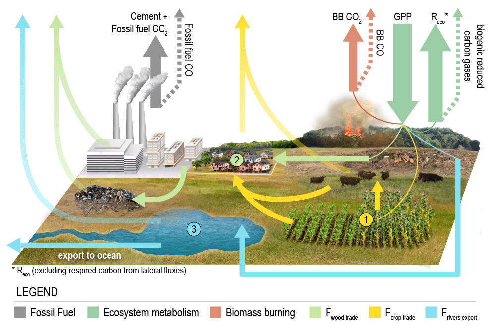
Figure 1CO2 is removed from the atmosphere through photosynthesis (GPP) and then emitted back to the atmosphere through a number of processes. Three processes move carbon laterally on Earth's surface such that emissions of CO2 occur in a different region than removals. (1) Agriculture: harvested crops are transported to urban areas and to livestock, which are themselves exported to urban areas. CO2 is respired to the atmosphere in livestock or urban areas. (2) Forestry: logged carbon is transported to urban and industrial areas, then emitted through decomposition in a landfill or combustion as a biofuel. (3) Water cycle: carbon is leached from soils into water bodies, such as lakes. The carbon is then either deposited, released to the atmosphere or transported to the ocean (Regnier et al., 2022). Arrows show carbon fluxes, and colors indicate whether the flux is associated with (grey) fossil fuel emissions, (dark green) ecosystem metabolism, (red) biomass burning, (light green) forestry, (yellow) agriculture or (blue) the water cycle. Semi-transparent arrows show fluxes that move between the surface and atmosphere, while solid arrows show fluxes that move between land regions. Dashed arrows show surface–atmosphere fluxes of reduced carbon species that are oxidized to CO2 in the atmosphere. For simplicity, a cement carbonation sink, volcano emissions and a weathering sink are not included in this figure.
Globally, there is a long-term net uptake of atmospheric CO2 by the land (approximately −6.6 Pg CO2 yr−1 or −1.8 Pg C yr−1 over 2010–2019; Canadell et al., 2021), which is the residual of an emission due to net land-use change (5.9±2.6 Pg CO2 yr−1 or 1.6±0.7 Pg C yr−1 over 2010–2019; Canadell et al., 2021) and removal by other terrestrial ecosystems (12.6±3.3 Pg CO2 yr−1 or 3.4±0.9 Pg C yr−1 over 2010–2019; Canadell et al., 2021). This removal is partially driven by direct feedbacks between increasing CO2 and the biosphere, such as CO2 fertilization of photosynthesis and increased water use efficiency. Carbon–climate feedbacks also lead to both increases and decreases in terrestrial carbon stocks: for example, warming at high latitudes leads to a more productive biosphere, but it also leads to increased plant and soil respiration (Kaushik et al., 2020; Walker et al., 2021; Canadell et al., 2021; Crisp et al., 2022). In addition, the release of nitrogen through anthropogenic energy and fertilizer use may drive increased carbon sequestration by the terrestrial biosphere (Schulte-Uebbing et al., 2022; Y. Liu et al., 2022; Lu et al., 2021). Regrowth of forests in previously cleared areas, especially in the extratropics, is also thought to be an important uptake term (Kondo et al., 2018; Cook-Patton et al., 2020). Currently, the relative impact of each of these contributions to long-term terrestrial carbon sequestration is poorly known and likely varies between biomes and climates.
While the existence of a long-term global land sink is supported through a number of lines of evidence (Ballantyne et al., 2012; Keeling and Graven, 2021), regional-scale emissions and removals are less well quantified. Regional-scale carbon sequestration can differ substantially from the global mean and can be impacted by the regional climate, disturbance events (Frank et al., 2015; Wang et al., 2021) and anthropogenic activities (Caspersen et al., 2000; Harris et al., 2012). The need to better quantify regional-scale emissions and removals of carbon has motivated much of the recent expansion of in situ CO2 observing networks, the launch of space-based CO2 observing systems and the development of CO2 inversion systems.
1.3 Background on atmospheric CO2 inversions
Atmospheric CO2 inversions estimate the underlying net surface–atmosphere CO2 fluxes from atmospheric CO2 observations, and this is what is meant by the top-down approach (Bolin and Keeling, 1963; Tans et al., 1990; Enting et al., 1995; Gurney et al., 2002; Peiro et al., 2022). In this approach, an atmospheric chemical transport model (CTM) is employed to relate surface–atmosphere CO2 fluxes to observed atmospheric CO2 mole fractions. As an inverse problem, the upwind CO2 fluxes are estimated from the downwind observed CO2 mole fractions. The surface CO2 fluxes are adjusted so that forward-simulated CO2 mole fractions better match the CO2 measurements while considering the uncertainty statistics on the observations, transport and prior surface fluxes.
The atmospheric CO2 inversion problem is generally ill-posed such that the solution is underdetermined by the observational constraints. In this case, additional information is required to produce a unique solution and prevent overfitting of the data (Lawson and Hanson, 1995; Tarantola, 2005). Typically, this is performed using Bayesian inference, where prior mean fluxes and their uncertainties provide additional information required to estimate fluxes (Rayner et al., 2019). Prior mean fluxes of net ecosystem exchange are usually obtained from terrestrial biosphere models (such as CASA, ORCHIDEE and CARDAMOM), while prior mean air–sea fluxes are derived from surface water partial pressure of CO2 (pCO2) datasets or from ocean models (e.g., Peiro et al., 2022). The resulting posterior flux estimates combine the constraints on surface fluxes from atmospheric CO2 data with the prior knowledge of the fluxes. If there is a high density of assimilated CO2 observations, then the posterior fluxes will be more strongly impacted by the assimilated data, whereas, in regions with sparse observational coverage, the posterior fluxes will generally remain similar to the prior fluxes (assuming similar prior flux uncertainties across regions).
Measurements of atmospheric CO2 best inform diffuse biosphere–atmosphere fluxes on large spatial scales. This is because CO2 has a long atmospheric lifetime such that the perturbation to atmospheric CO2 due to emissions and removals from individual processes and locations gets mixed in the atmosphere (Gloor et al., 2001; Liu et al., 2015). For example, the measurements of CO2 at Mauna Loa, Hawaii, provide a good estimate of the global-scale changes of CO2 surface fluxes. Inferring smaller-scale flux signals requires a high density of CO2 observations (to capture gradients in atmospheric CO2) and accurate modeling of atmospheric transport (to relate the measurements with surface fluxes). The accuracy of flux estimates depends on a number of factors, particularly the accuracy and precision of the data, transport model and prior constraints. Stringent requirements on the accuracy of space-based column-averaged dry-air mole fraction () retrievals are required to infer surface fluxes (Chevallier et al., 2005a; Miller et al., 2007). Biases in retrievals from the Orbiting Carbon Observatory (OCO-2) related to spectroscopic errors, solar zenith angle, surface properties, and atmospheric scattering by clouds and aerosols have been identified (Wunch et al., 2017b). However, intensive research has reduced retrieval errors over time (O'Dell et al., 2018; Kiel et al., 2019). As will be shown in Sect. 4.1, biases in OCO-2 retrievals over land are thought to be relatively small, although regionally structured biases may be present. However, OCO-2 retrievals over oceans may contain more large-scale spatially coherent retrieval errors that can adversely impact flux estimates.
Accurate atmospheric transport is critical for correctly relating surface–atmosphere fluxes to observations. Due to computational constraints, CTMs are typically run offline with coarsened meteorological fields relative to the parent numerical weather prediction model, which has been shown to introduce systematic transport errors in some configurations (Yu et al., 2018; Stanevich et al., 2020). In addition, these offline CTMs have been shown to have large-scale systematic differences in transport associated with the implementation of transport algorithms (Schuh et al., 2019, 2022). These errors appear to be of the same order as the retrieval biases, although the patterns in time and space are different. Systematic errors related to model transport (and errors in prior information) can partially be accounted for by performing multiple inversions that differ in CTM and prior constraints employed. This motivates inversion model intercomparison projects (MIPs), such as the OCO-2 MIP project (see Sect. 3.2; Crowell et al., 2019; Peiro et al., 2022). From these ensembles of inversions, estimates of both systematic errors (accuracy) and random errors (precision) can be obtained from the model spread.
In this work, we focus on the carbon budget of Earth's land area, including aquatic systems such as rivers and lakes. In particular, we consider fluxes of carbon between the land and the atmosphere and lateral carbon transport processes on land and between the land and ocean (Fig. 1). We define the following annual net carbon fluxes (see Fig. 2 for a schematic representation of these fluxes):
-
Fossil fuel and cement emissions (FF). The burning of fossil fuels and release of carbon due to cement production, representing a flux of carbon from the land surface (geologic reservoir) to the atmosphere.
-
Net biosphere exchange (NBE). Net flux of carbon from the terrestrial biosphere to the atmosphere due to biomass burning (BB) and Reco minus gross primary production (GPP) (i.e., ). It includes both anthropogenic processes (e.g., deforestation, reforestation, farming) and natural processes (e.g., climate-variability-induced carbon fluxes, disturbances, recovery from disturbances).
-
Terrestrial net carbon exchange (NCE). Net flux of carbon from the surface to the atmosphere. For land, NCE can be defined as
-
Lateral crop flux (Fcrop trade). The lateral flux of carbon in (positive) or out (negative) of a region due to agriculture.
-
Lateral wood flux (Fwood trade). The lateral flux of carbon in (positive) or out (negative) of a region due to wood product harvesting and usage.
-
Lateral river flux (Frivers export). The lateral flux of carbon in (positive) or out (negative) of a region transported by the water cycle.
-
Net terrestrial carbon stock loss (ΔCloss). Positive values indicate a loss (decrease) of terrestrial carbon stocks (organic matter stored on land), including above- and below-ground biomass in ecosystems and biomass contained in anthropogenic products (lumber, cattle, etc.). This is calculated as
-
Net terrestrial carbon stock gain (ΔCgain). Positive values indicate a gain (increase) of terrestrial carbon stocks, and this is the negative of ΔCloss:
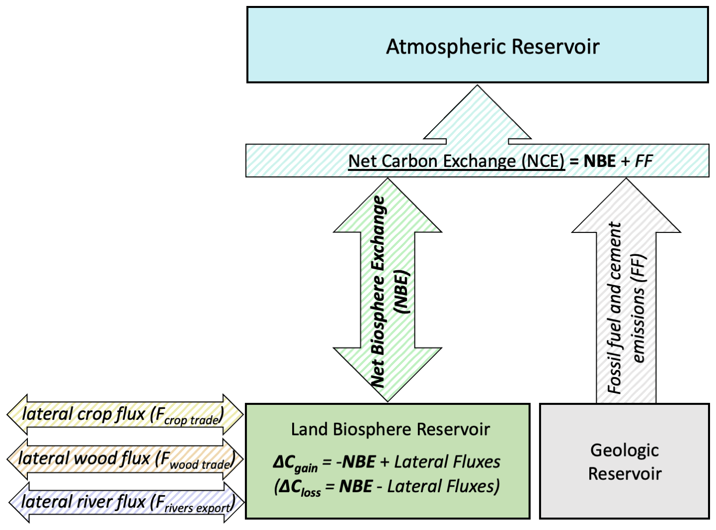
Figure 2Carbon fluxes for a given land region, such as a country. Boxes with solid backgrounds show reservoirs of carbon. Arrows with hatched shading show fluxes between reservoirs. NCE is underlined to emphasize that this quantity is estimated from the atmospheric CO2 measurements using top-down methods. Italicized quantities are obtained from bottom-up datasets (FF, Fcrop trade, Fwood trade, Frivers export). Bold quantities are derived in this study from the top-down and bottom-up datasets (NBE, ΔCgain, ΔCloss).
Country and regional aggregation
To aggregate gridded 1∘ × 1∘ flux estimates to country totals we use a country mask (Center for International Earth Science Information Network – CIESIN – Columbia University, 2018). We also provide NCE and ΔCloss estimates for several country groupings. A number of regional intergovernmental organizations are included: the Association of Southeast Asian Nations (ASEAN), the African Union (AU) and each of its sub-regions (North, South, West, East and Central), the Community of Latin American and Caribbean States plus Brazil (CELAC+Brazil), the Economic Cooperation Organization (ECO), the European Union (EU or EU27), and the South Asian Association for Regional Cooperation (SAARC). We also include some geographic regions, specifically North America, the Middle East and Europe. Countries included in these groupings are listed in the Supplement (Text S1).
Here, we describe the methodologies and datasets for estimating FF (Sect. 3.1), NCE (Sect. 3.2) and lateral carbon fluxes (Sect. 3.3), as well as how these data are used to estimate ΔCloss (Sect. 3.4).
3.1 Fossil fuel and cement emissions
Gridded 1∘ × 1∘ fossil CO2 emissions, including those from cement production, are calculated as follows. Monthly gridded emissions up to 2019 are taken from the 2020 version of the Open-source Data Inventory for Anthropogenic CO2 (ODIAC2020, 2000–2019) emission data product (Oda and Maksyutov, 2011; Oda et al., 2018). The 2020 emissions were not part of ODIAC but were projected using the Carbon Monitor (CM) emission data product (https://carbonmonitor.org/, last access: 19 May 2021). For each month in 2020 and later, the ratio between that month's emissions and the emissions from the same month in 2019 was calculated from the CM emission data. Since CM provides daily emissions per sector for a handful of major emitting countries and the globe, CM emissions are summed over sectors and days in each month to create monthly total emissions per named country and the rest of the world (RoW). The ratio of each (post-2019) month's emission to the same month in 2019 is then calculated per named country and RoW, then distributed over a 1∘ × 1∘ grid assuming homogeneity of the ratio over each named country and RoW. The 2019 ODIAC emissions for that month are then multiplied by the ratio to generate 1∘ × 1∘ monthly emissions after 2019. While this method loses the information of day-to-day variability provided by CM, this is a conscious choice to be consistent over the entire inversion period. Finally, we impose day-of-week and hour-of-day variations on these fluxes following the Temporal Improvements for Modeling Emissions by Scaling (TIMES) diurnal and day-of-week scaling (Nassar et al., 2013). The 1∘ × 1∘ uncertainty map is based on the combination of the global level FF uncertainty (1σ of 4.2 %, Andres et al., 2014) and the grid level emission differences due to the different disaggregation methods (Oda et al., 2015). Note that these FF uncertainties are not considered in the inversions used for this product development.
Country-level fossil fuel emission estimates are obtained by aggregating the 1∘ × 1∘ estimates using the country mask. Uncertainties on country-level estimates are calculated using the fractional uncertainties of Andres et al. (2014).
3.2 Net carbon exchange (NCE) and net biosphere exchange (NBE)
We employ results from the v10 OCO-2 MIP, which is an international collaboration of atmospheric CO2 inversion modelers that produces ensembles of CO2 surface–atmosphere flux estimates by assimilating space-based OCO-2 retrievals of and in situ CO2 measurements. The v10 OCO-2 MIP is updated from the v9 OCO-2 MIP described in Peiro et al. (2022). Updates to the v10 OCO-2 MIP are presented here with additional details available at https://gml.noaa.gov/ccgg/OCO2_v10mip/ (last access: 6 February 2023).
(Philip et al., 2019, 2022)(D. F. Baker et al., 2006; Baker et al., 2010)(Chevallier et al., 2005b)(J. Liu et al., 2021)(Z. Liu et al., 2022)(Jacobson et al., 2020)(Miller et al., 2020)(Chen et al., 2021b, a)(Weir et al., 2021a, b)(Maksyutov et al., 2021)(Deng et al., 2014, 2016)(Zammit-Mangion et al., 2022)Table 1Inversion specifications for each v10 OCO-2 MIP ensemble member. Note that since the creation of this table, the Global Carbon Assimilation System (GCAS; Jiang et al., 2021) has also contributed an ensemble member.
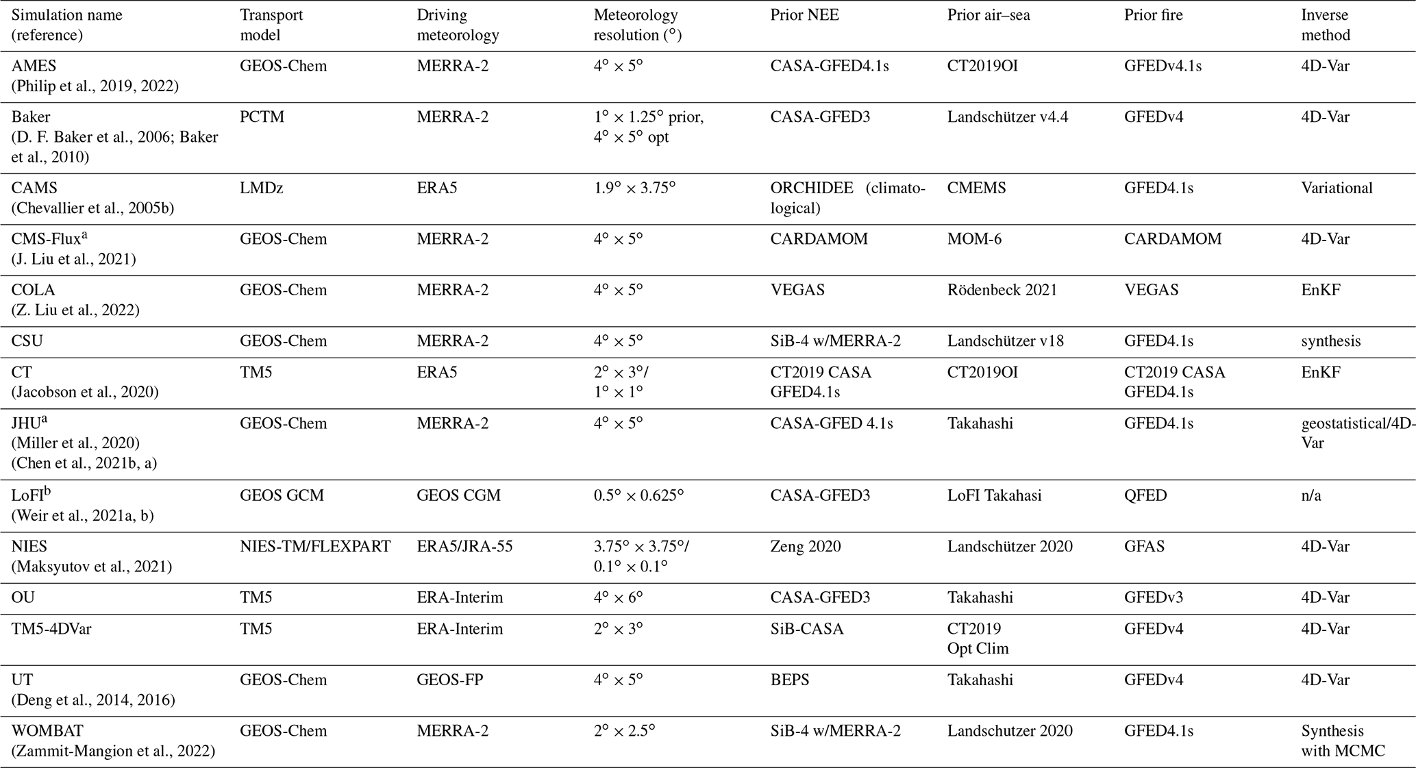
a Due to time constraints, this ensemble member is not included in this product. b This is not a traditional inversion and is not included in this product. n/a: not applicable.
The v10 OCO-2 MIP consists of a number of inversion systems that perform a set of experiments following a standard protocol. Here, we include fluxes from 11 of the 14 MIP models (Table 1; CMS-Flux and JHU were excluded due to time constraints, and LoFI was excluded because it employs a non-traditional inversion approach that does not follow the MIP protocol). There are five v10 OCO-2 MIP experiments that each ensemble member performs, which differ by the data that are assimilated (CO2 datasets described in Sect. 3.2.1):
-
IS assimilates in situ CO2 mole fraction measurements from an international observational network.
-
LNLG assimilates ACOS v10 land nadir and land glint total column dry-air mole fractions () from OCO-2.
-
LNLGIS assimilates both in situ and ACOS v10 OCO-2 land nadir and glint retrievals together.
-
OG assimilates ACOS v10 OCO-2 ocean glint retrievals
-
LNLGOGIS assimilates all the above datasets together.
For each experiment, each inversion group imposes a common fossil fuel emission dataset identical to the one described in Sect. 3.1. All other prior flux estimates were chosen independently by each modeling group and are listed in Table 1. The inversions assimilate the standardized v10 OCO-2 and in situ data from 6 September 2014 through 31 March 2021 (see Sect 3.2.1), with the length of spin-up period and in situ data assimilated during that period being left up to the discretion of each group in the MIP. Each modeling group submitted net air–sea fluxes and NBE across 2015–2020, interpolated from the native resolution to a 1∘ × 1∘ spatial grid at monthly resolution, which are publicly available for download from https://gml.noaa.gov/ccgg/OCO2_v10mip/ (last access: 6 February 2023).
The performance of each atmospheric CO2 inversion was evaluated through comparisons of the posterior CO2 mole-fraction field (i.e., CO2 fields simulated forward with the posterior fluxes) against independent in situ CO2 measurements and OCO-2 retrievals that were withheld from the assimilation for validation, as well as retrievals from the Total Column Carbon Observing Network (TCCON; Wunch et al., 2011). The evaluation of the experiments is presented in Sect. 4, with additional analysis available from the v10 OCO-2 MIP website.
For this study, the best estimate of NCE is taken to be the ensemble median for each experiment (denoted ). The uncertainty in NCE is calculated as an estimate (denoted σNCE) of the distribution's standard deviation using the interquartile range (IQR) of the v10 OCO-2 MIP ensemble. It is a robust estimate that requires only the middle 50 % of the ensemble to be normally distributed (Hoaglin et al., 1985). Hence from the normal tables, to two decimal places,
For country-level fluxes, the NCE estimates are first aggregated to country totals for each ensemble member before calculating the median and standard deviation. This is done because there are spatial covariances between 1∘ × 1∘ grid cells. Thus, first aggregating regions for each ensemble member accurately propagates the aggregate differences between regions across the ensemble members.
The NBE estimate is calculated by subtracting the ODIAC fossil fuel emissions from NCE. The variance in NBE is then taken to be the sum of the variances of NCE and FF:
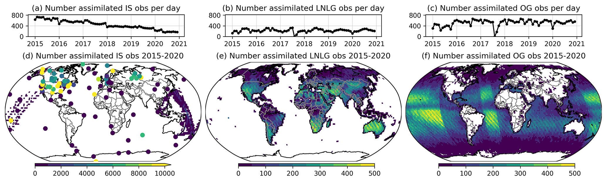
Figure 3Assimilated observations for IS, LNLG and OG v10 MIP experiments. Number of monthly (a) in situ CO2 measurements and (b) ACOS v10 OCO-2 land nadir and land glint retrievals binned into 10 s averages and (c) ACOS v10 OCO-2 ocean glint retrievals binned into 10 s averages. Spatial distribution of (d) in situ (e) ACOS v10 OCO-2 land retrievals and (f) ACOS v10 OCO-2 ocean retrievals over 2015–2020. Shipboard and aircraft in situ CO2 measurements are aggregated to a 2∘ × 2∘ spatial grid, surface site measurements are shown as scattered points and ACOS v10 OCO-2 retrievals are shown aggregated to a 2∘ × 2∘ spatial grid.
3.2.1 Atmospheric CO2 data included in v10 OCO-2 MIP
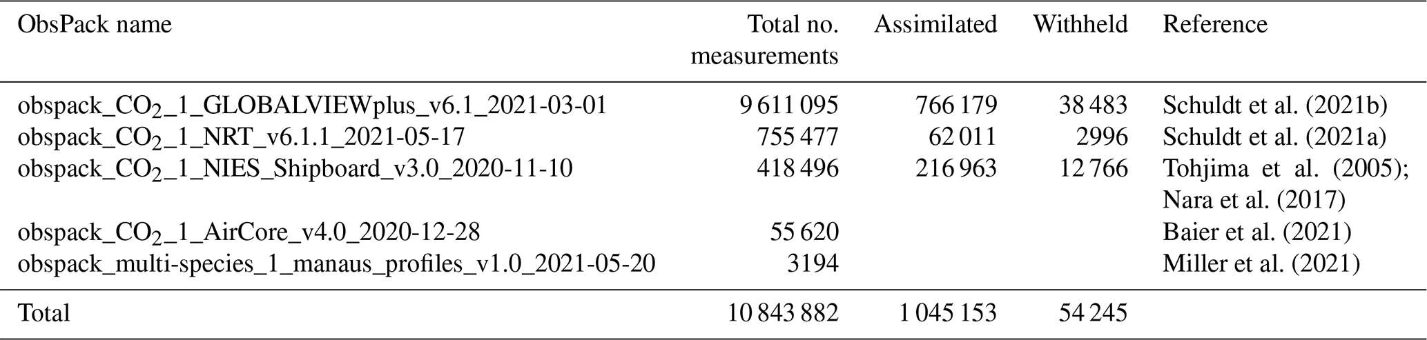
In situ CO2 measurements (Fig. 3a and d) are drawn from five data collections made available in ObsPack format (Masarie et al., 2014). Those source ObsPacks and their references are listed in Table 2. These data include measurements from 55 international laboratories at 460 sites around the world. The majority of data are from the openly available GLOBALVIEW+ program but with some additional provisional data for 2020–2021 and data from other programs not participating in the GLOBALVIEW+ project. CO2 measurements are broadly divided into two categories: those measurements we identify as suitable for assimilation and other measurements not suitable for assimilation.
Schuldt et al. (2021b)Schuldt et al. (2021a)Tohjima et al. (2005); Nara et al. (2017)Baier et al. (2021)Miller et al. (2021)Table 2In situ CO2 measurement collections used in the v10 OCO-2 MIP, with the total number of measurements between 6 September 2014 and 1 January 2021 and the numbers of measurements assimilated and withheld for cross-validation in the same period. More than 95 % of the in situ measurements come from the GLOBALVIEW+ and CO2 NRT ObsPacks, both of which are publicly available at https://gml.noaa.gov/ccgg/obspack/data.php.
In CO2 inverse analyses, uncertainties ascribed to in situ measurements are a combination of the uncertainty in the measurement and a representativeness error from the inability of the forward model to accurately simulate the measurement (due to aspects like a coarse model grid). To characterize the representativeness error, we used an empirical scheme based on simulations from the v7 OCO-2 MIP (Crowell et al., 2019). In situ CO2 measurements are simulated in a forward simulation, and then the model–data mismatch statistics are calculated to characterize the representativeness errors at each measurement location and for each season. Although this was the standard method for characterizing uncertainties for modeled in situ measurements, each v10 OCO-2 MIP group was free to choose how to set the uncertainties in their specific setups.
Of the in situ measurements designated as being appropriate for assimilation, about 5 % were withheld for cross-validation purposes. These data were chosen to be as independent as possible from the measurements that were assimilated. For quasi-continuous measurements, such as those taken every 15 min at NOAA tall towers, measurements were withheld for entire days: we chose 5 % of the days in the dataset, and we withheld every assimilable measurement on that day. This is also how CO2 measurements on National Institute for Environmental Studies (NIES) ships were treated. Entire aircraft profiles in the NOAA light-aircraft profiling network are assumed to consist of vertically correlated measurements, so entire profiles were withheld: we chose 5 % of aircraft profiles to withhold. Most flask sites have measurement sampling protocols intended to ensure independence; they are often taken at weekly or biweekly intervals during meteorological conditions meant to allow regional background air masses to be sampled. Thus, we chose to withhold 5 % of assimilable flask measurements. We also verified that datasets at the same site were withheld on the same days; aircraft profiles over tower sites were, for instance, withheld on the same days that tower data were withheld.
OCO-2 land (Fig. 3b and e) and ocean (Fig. 3c and f) retrievals are performed using version 10 of NASA's ACOS full-physics retrieval algorithm (O'Dell et al., 2018). A common set of OCO-2 retrieval “super-obs” data were derived from these retrievals and were assimilated by each modeling group. These super-obs are obtained by aggregating retrievals into 10 s averages (which better match the coarse transport models' grid cells used in the inversions) following the same procedure as the v9 OCO-2 MIP (Peiro et al., 2022). Specifically, individual scenes within the 10 s span are weighted according to the inverse of the square of the uncertainty (standard deviations) produced by the retrieval, and correlations of +0.3 for land scenes and +0.6 for ocean scenes are assumed when calculating the uncertainty on the 10 s averages (see Sect. 3.2.1 of Baker et al., 2022); transport model errors are also considered (based on Schuh et al., 2019). Only 10 s spans with 10 or more good quality retrievals were used (sparser data being thought to be more prone to cloud-related biases). In the same vein as was done for the in situ data, data from 5 % of the orbits (entire orbits were withheld), chosen at random, were withheld for evaluation purposes.
3.3 Lateral carbon fluxes
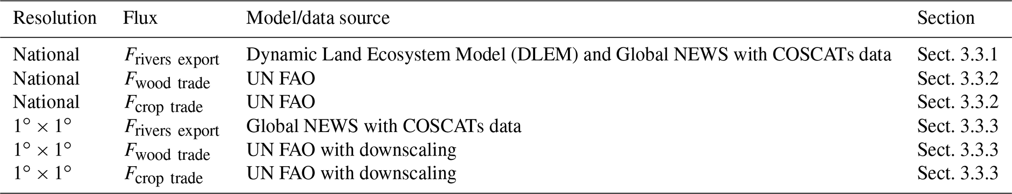
Lateral carbon flux datasets (Table 3) include country-level Frivers export (Sect. 3.3.1), country-level Fcrop trade and country-level Fwood trade (Sect. 3.3.2). Gridded lateral fluxes are estimated using a somewhat different approach and are described in Sect. 3.3.3.
3.3.1 Country-level Frivers export
Rivers transport carbon laterally across land regions (e.g., to a lake) and from the land to the ocean. This lateral transport must be accounted for to quantify the total change in terrestrial carbon in a given region. However, there is considerable uncertainty in lateral carbon flux by rivers. To account for this, we use two independent estimates of country-level totals: one from the Dynamic Land Ecosystem Model (DLEM; Tian et al., 2010, 2015a) and the other based on Deng et al. (2022), who use the Global NEWS model (Mayorga et al., 2010) and observations across COastal Segmentation and related CATchments (COSCATs; Meybeck et al., 2006) that include dissolved inorganic carbon (DIC) of atmospheric origin, dissolved organic carbon (DOC) and particulate organic carbon (POC). These datasets cover 2015–2019. For 2020, we impose the 2015–2019 mean.
The DLEM is a process-based terrestrial ecosystem model that couples biophysical, soil biogeochemical, plant physiological and riverine processes with vegetation and land-use dynamics to simulate and predict the vertical fluxes, lateral fluxes, and storage of water, carbon, GHGs, and nutrient dynamics in terrestrial ecosystems and their interfaces with the atmosphere and land–ocean continuum (Tian et al., 2010, 2015a). There are three major processes involved in simulating the export of water, carbon and nutrients from land surface to the coastal ocean: (1) the generation of runoff and leachates; (2) the leaching of water, carbon, and nutrients from land to river networks in the form of overland flow and base flow; and (3) transport of riverine materials along river channels from upstream areas to coastal regions. The key processes and parameterization in the DLEM have been described in previous publications regarding the water discharge (Liu et al., 2013; Tao et al., 2014), riverine carbon fluxes (Ren et al., 2015, 2016; Tian et al., 2015b; Yao et al., 2021) and riverine nitrogen fluxes (Yang et al., 2015; Tian et al., 2020) from the terrestrial ecosystem to coastal oceans. The newly improved DLEM aquatic module better addresses processes within global small streams, which were recognized as hotspots of GHG emissions (Yao et al., 2020, 2021). DLEM produces estimates of the land loadings of carbon species (DIC, DOC and POC), CO2 degassing and carbon burial during transporting, and the exports of carbon (DIC, DOC and POC) to the ocean for 105 basin-level segmentations (modified from COSCATs) (Meybeck et al., 2006). To estimate country totals, we map the basin carbon loss across land by assuming that the net carbon flux occurs uniformly across each basin. We then use the country mask to estimate the country totals for each region.
Deng et al. (2022) estimate the lateral carbon export by rivers to the coast minus the imports from rivers entering in each country (for relevant cases), including DOC, POC and DIC of atmospheric origin. Estimates of DOC, POC and DIC are obtained from the Global NEWS model (Mayorga et al., 2010), with a correction based on Resplandy et al. (2018) so that the global total exported to the coastal ocean is 2.86 Pg CO2 yr−1 (0.78 Pg C yr−1). Deng et al. (2022) perform a correction to the Global NEWS estimates to remove the contribution of lithogenic carbon, using the methodology of Ciais et al. (2021).
For the analysis that follows, we estimate country-level totals of riverine lateral carbon fluxes by combining the estimates of DLEM with those of Deng et al. (2022). We take the mean of the two estimates to be the best estimate and take the magnitude of the difference between the estimates to be the 1σ uncertainty. Figure S1 shows the 2015–2019 mean annual net riverine lateral carbon fluxes. Fluxes are uniformly negative, implying a net flux of carbon from the land to the ocean and reduction in stored carbon for all countries. Fluxes are most negative in tropical rain forest and tropical monsoon climates, and they are smallest in more arid regions.
3.3.2 Country-level Fwood trade and Fcrop trade
Wood and crop products are traded between nations. We estimate the annual lateral fluxes of carbon due to this trade following the approaches of Deng et al. (2022) and Ciais et al. (2021). This approach utilizes crop and wood trade data compiled by the Food and Agriculture Organization of the United Nations (FAO; http://www.fao.org/faostat/en/#data, last access: 6 February 2023). The crop flux was estimated from the annual trade balance of 171 crop commodities calculated for each country. For wood products, we use the bookkeeping model of Mason Earles et al. (2012) to calculate the fraction of imported carbon in wood products that is oxidized in each of 270 countries during subsequent years. The 1σ uncertainties in country-level fluxes are assumed to be 30 % of the mean value. This dataset covers 2015–2019. For 2020, we assume fluxes equal to the 2015–2019 mean. The net crop and wood lateral fluxes and their uncertainties are shown in Fig. S2.
3.3.3 1∘ × 1∘ lateral flux estimates
Lateral fluxes at a higher resolution (1∘ × 1∘) follow similar principles to national values but were estimated separately with different implementation choices. High-resolution proxy data (satellite-derived NPP, population or livestock maps, etc.) enabled sub-national disaggregation. This was done using national totals based on FAO statistics for Fwood trade and Fcrop trade. For Frivers export these estimates were generated from Global NEWS and COSCATs data (DLEM was only used for national totals). For each 1∘ × 1∘ grid cell, we assume the standard deviation of the mean flux to be 30 % for Fwood trade and Fcrop trade and 60 % for Frivers export. These uncertainty estimates are based on expert opinion, as a rigorous error budget has not yet been developed for the 1∘ × 1∘ lateral flux estimates.
3.4 Estimate of carbon stock loss (ΔCloss)
Finally, we calculate ΔCloss using Eq. (2) with the datasets described above. Assuming that the components contributing to ΔCloss are independent, we calculate the uncertainty on ΔCloss by combining the uncertainties (1 standard deviations) from the component fluxes in quadrature:
The performance of top-down CO2 flux estimates can be impacted by a number of factors, including biases in the assimilated data, model transport, prior constraints and inversion architectures. Therefore, evaluating the performance of v10 OCO-2 MIP fluxes against independent observational datasets is critical for assuring high-quality flux estimates. Here, we evaluate the v10 OCO-2 MIP experiments in two ways. First, we compare the posterior CO2 fields against independent CO2 measurements (Sect. 4.1). Second, we compare the inferred air–sea CO2 flux against estimates based on surface ocean CO2 partial pressure (pCO2) measurements (Sect. 4.2).
4.1 Evaluation of posterior CO2 fields
We consider four atmospheric CO2 datasets:
-
Withheld in situ CO2 measurements. These are measurements contained in the ObsPack collection described in Sect. 3.2.1 but intentionally withheld for evaluation purposes. Independence from the assimilated data is ensured following the steps described in Sect. 3.2.1.
-
retrievals from the TCCON. These data are acquired from a network of ground-based Fourier transform spectrometers measuring direct solar spectra from which is retrieved (Wunch et al., 2011). For this analysis, we include 30 TCCON sites listed in Table A1. These data are filtered and aggregated following the method outlined in Appendix C of Crowell et al. (2019).
-
Withheld OCO-2 land glint and land nadir retrievals. These data could have been assimilated, but they are intentionally withheld for evaluation purposes (Sect. 3.2.1).
-
Withheld OCO-2 ocean glint retrievals. These data could have been assimilated, but they are intentionally withheld for evaluation purposes (Sect. 3.2.1).
We first perform a simple check on the inversion results by comparing the atmospheric CO2 growth rate estimated from the v10 OCO-2 MIP experiments to that derived directly from NOAA CO2 measurements (Fig. 4). The growth rate is estimated from CO2 measurements and model co-samples at “marine boundary layer” sites, which predominantly observe well-mixed marine boundary layer air representative of a large volume of the atmosphere. A smooth curve is then fit to these data to estimate the global growth rate (Thoning et al., 1989). This is the same method employed by NOAA to report the CO2 growth rate (http://www.gml.noaa.gov/ccgg/trends/, last access: 6 February 2023). We estimate the uncertainty in the measurement-based growth rate from the difference between the growth rate estimated here and that reported on the NOAA website. Differences between these estimates are primarily driven by differences in measurement sampling used for the website relative to that used here (as we are limited to withheld co-samples here). We calculate the uncertainty as the standard error of the mean for the differences between the growth rates estimated here and by NOAA across 2015–2019. This gives an uncertainty on the 5-year growth rate of ±0.053 ppm yr−1. Note that NOAA reports the growth rate using the X2019 scale, whereas our estimates here are from the X2007 scale, which may contribute to the differences. We find that the IS, LNLG and LNLGIS experiments show good agreement with the NOAA estimate over this period. However, both the OG and LNLGOGIS experiments are found to have a high bias. This suggests that there may be a spurious trend in the v10 OCO-2 ocean glint retrievals of 0.04–0.13 ppm yr−1 (OG experiment bias) that impacts flux estimates in both experiments that assimilate ocean glint data.
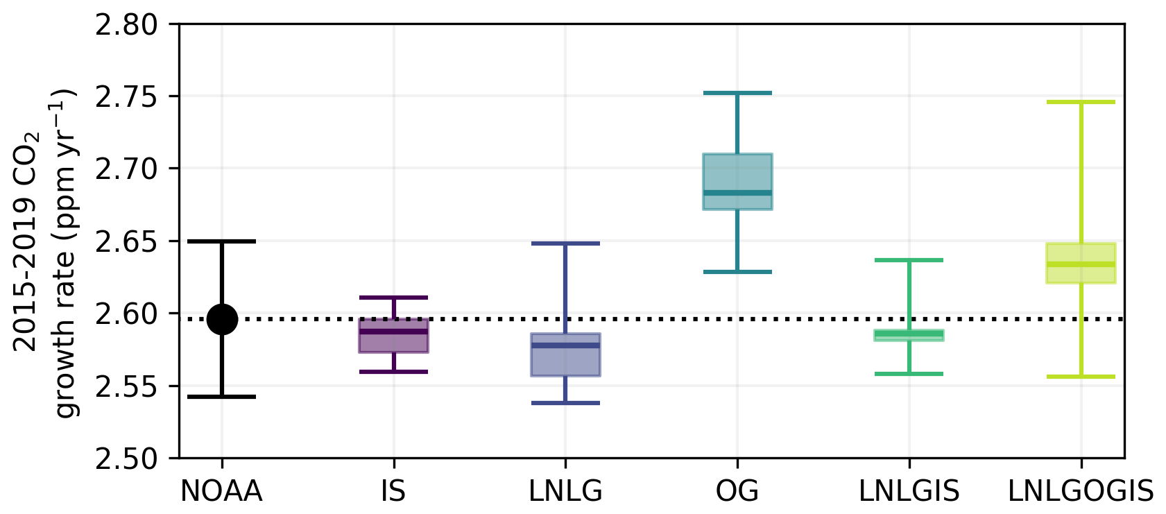
Figure 42015–2019 global mean CO2 growth rate estimated from NOAA site measurements and for the v10 OCO-2 MIP experiments. The estimates of the CO2 growth rate for each experiment are computed by sampling the model CO2 fields at the same times and locations as those used to derive the NOAA measurement-based estimate. Each v10 OCO-2 MIP experiment is shown as a box plot, with the error bars showing the full range, the shaded region showing the interquartile range and the solid line showing the median ensemble member of the ensemble.
Second, we estimate the overall observation–model agreement as the root mean square error (RMSE) for the withheld in situ CO2, TCCON , withheld OCO-2 land and withheld OCO-2 ocean (Fig. 5). For the in situ and OCO-2 data, the normalized RMSE is shown, meaning that the observation–model difference is divided by the observational uncertainty (1σ). Overall, we find reasonably good agreement between the evaluation datasets and posterior fields for all experiments. The OG experiment gives the largest RMSEs against the withheld in situ CO2, TCCON and OCO-2 land . This provides further evidence that the ocean glint data may have some residual biases that adversely impact the flux estimates.
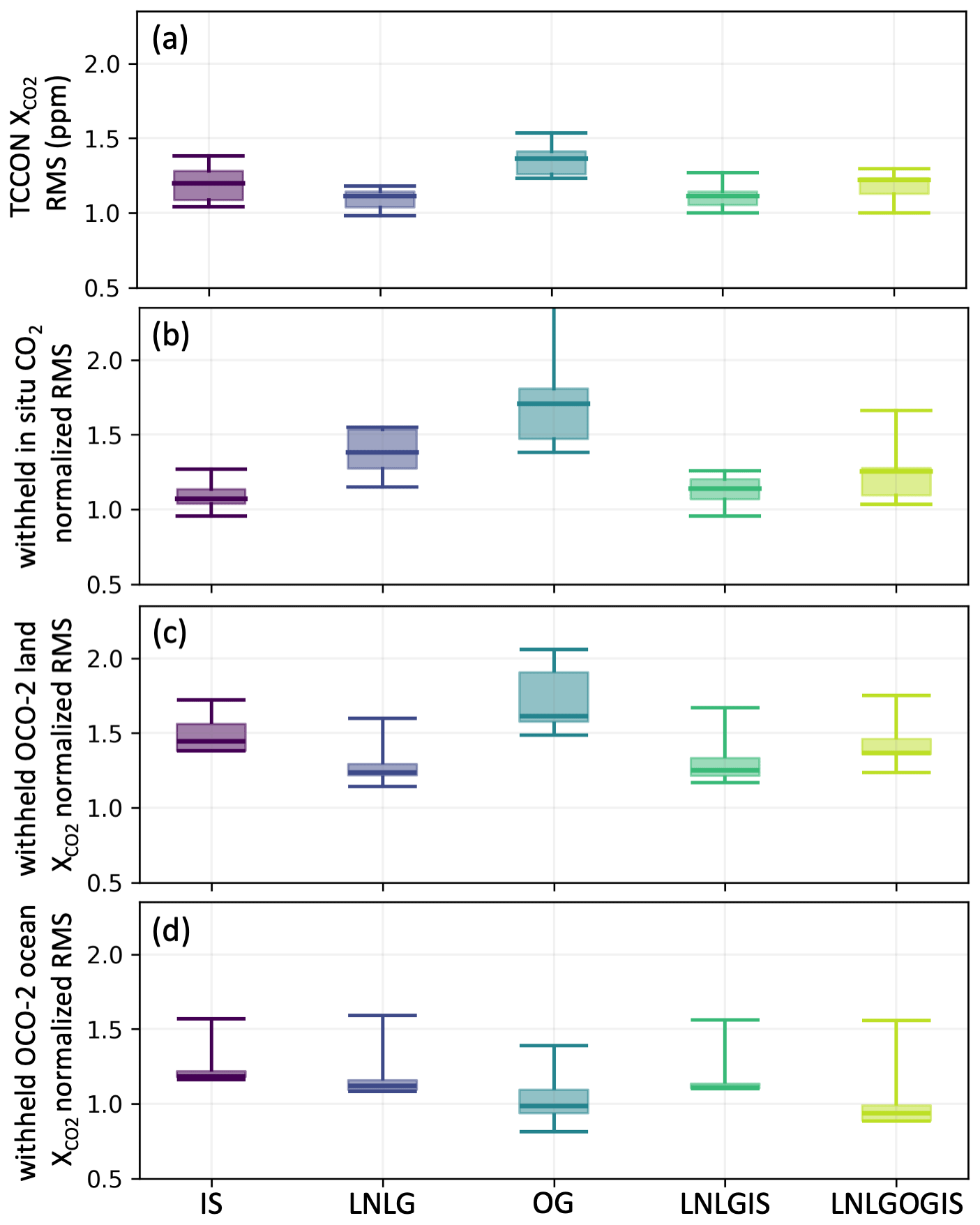
Figure 52015–2020 root mean square error (RMSE) between the v10 OCO-2 MIP experiments and (a) TCCON retrievals, (b) withheld in situ CO2 measurements, (c) withheld OCO-2 land retrievals, and (d) withheld OCO-2 ocean retrievals. For the comparisons with withheld in situ and OCO-2 observations, the normalized RMSE estimate is plotted (that is, the observation–model mismatch is divided by the observational uncertainty). Note that NIES IS and CSU co-samples are not available and not included in this plot.
Finally, we examine the mean bias over 2015–2020 for 30∘ latitude bins (Fig. 6). Similar to previous comparisons, we find that the OG experiment stands out as being more biased against the independent observations relative to the other experiments. In particular, the observation–model difference for the OG experiment tends to be lower (higher modeled CO2) than the evaluation datasets. This is particularly evident in the northern extratropics. Over 30–60∘ N, where independent observations are densest, we find that the OG ensemble median is biased by −0.69 ppm against TCCON, −0.74 ppm against withheld in situ and −0.48 ppm against withheld OCO-2 LNLG, suggesting a possible meridional bias (higher retrieved than independent observations) in the OCO-2 ocean retrievals. The IS, LNLG and LNLGIS experiments tend to show similar observation–model differences, suggesting limited ability to distinguish between the performance of these inversions in large-scale features.
All experiments show some biases against TCCON sites. In particular, low biases (high modeled CO2) are found for 0–30∘ S and 60–90∘ N. The underlying cause for these differences is unknown. Figure S3 shows the monthly mean observation–model differences for each TCCON site and each experiment. The differences can be quite variable between sites but are generally similar between experiments (for IS, LNLG and LNLGIS). Some of these differences may be related due to representativeness errors, particularly for urban sites. For example, Caltech and JPL are within Los Angeles County and show a large positive bias, while nearby Edwards is less impacted by urban emissions and shows a much smaller bias (Schuh et al., 2021). However, other differences are harder to explain, such as a negative trend in the observation–model bias for Park Falls and positive at Darwin during the 2015–2020 period. Site-to-site biases among TCCON sites may also contribute to these differences.

Figure 6Median bias (data minus model) over 30∘ latitude bins averaged over 2015–2020 for (a) TCCON retrievals, (b) withheld in situ CO2 measurements, (c) withheld OCO-2 land retrievals and (d) withheld OCO-2 ocean retrievals. Note that NIES IS and CSU co-samples are not available and not included in this plot.
Overall, this analysis finds that the OG experiment shows the poorest agreement against the evaluation datasets (excluding the withheld ocean glint data). The LNLGOGIS experiment shows the second worst performance against evaluation datasets, while the remaining experiments (IS, LNLG and LNLGIS) all show good agreement against the evaluation data. These results suggest that there may be residual biases in the OCO-2 ocean glint dataset that adversely impact the OG and LNLGOGIS experiments.
4.2 Comparison of air–sea fluxes with pCO2-based estimates
The exchange of CO2 between the atmosphere and the ocean (air–sea flux) can be estimated from measurements of the surface ocean partial pressure of CO2 (pCO2). These pCO2 data are extrapolated to global maps and combined with gas transfer velocity parameterizations to infer global maps of the air–sea CO2 fluxes (Fay et al., 2021). Although significant uncertainties remain, particularly in accurately representing the gas transfer velocity (Fay et al., 2021), comparisons between the pCO2-based air–sea fluxes and v10 OCO-2 MIP experiments can inform possible biases between estimates and inform potential areas for future research.
Here, we compare v10 OCO-2 MIP air–sea fluxes to an ensemble of air–sea flux estimates from SeaFlux (Fay et al., 2021; Gregor and Fay, 2021a). SeaFlux developed a standardized approach to harmonize and extend six air–sea CO2 flux products from as many surface pCO2 products: JENA-MLS (Rödenbeck et al., 2013), MPI-SOMFFN (Landschützer et al., 2014, 2020), CMEMS-FFN (Denvil-Sommer et al., 2019; Chau et al., 2022), CSIR-ML6 (Gregor et al., 2019), JMA-MLR (Iida et al., 2021) and NIES-FNN (Zeng et al., 2014). For each pCO2 product, we examine the mean of three air–sea fluxes obtained using different wind reanalysis datasets to estimate the gas transfer parameterization (ERA5, JRA-55 and CCMP2). The spread among these six estimates provides a measure of uncertainty in the extrapolation of pCO2 data to a global grid but does not account for errors in the gas transfer velocity formulation nor the uncertainties in the reanalysis winds used as input (Fay et al., 2021). Note that the prior estimates of air–sea CO2 fluxes in v10 OCO-2 MIP experiments are generally pCO2-based flux estimates and therefore not independent from the SeaFlux datasets.
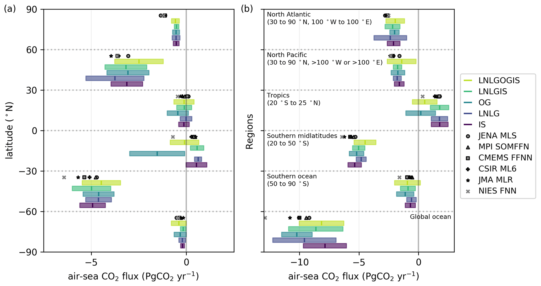
Figure 7(a) Zonal mean air–sea CO2 flux (positive values represent flux towards atmosphere) for 30∘ increments of latitude based on 1∘ × 1∘ estimates averaged over 2015–2019. (b) Air–sea CO2 flux for six large ocean regions. Colored bars show the MIP experiment results (median ± 1 standard deviation), and the symbols show the pCO2-based air–sea fluxes from the six SeaFlux products.
Figure 7 shows the 2015–2019 mean air–sea fluxes for each of the six SeaFlux products and for the v10 OCO-2 MIP experiments across 30∘ latitude bands and large ocean regions. Over the global ocean, the pCO2-based air–sea fluxes tend to give stronger removals ( Pg CO2 yr−1 or −2.7 Pg C yr−1, to −12.9 Pg CO2 yr−1 or −3.5 to −2.5 Pg C yr−1) than the v10 OCO-2 MIP, which range from Pg CO2 yr−1 ( Pg C yr−1) for the IS experiment to Pg CO2 yr−1 ( Pg C yr−1) for the OG experiment. On regional scales, the v10 OCO-2 MIP experiments overlap with the pCO2-based estimates except for the northern high latitudes (60–90∘ N), where pCO2-based estimates suggest systematically larger removals. Similarly, the pCO2-based estimates tend to give greater removals over the southern midlatitudes (20–50∘ S).
The different v10 OCO-2 MIP experiments tend to give similar air–sea fluxes, except for the OG experiment in the tropics. Although not systematic, the OG experiment suggests weaker emissions in the tropics of 0.2±1.3 Pg CO2 yr−1 (0.05±0.34 Pg C yr−1) relative to the median pCO2-based estimate of 1.6 Pg CO2 yr−1 (0.43 Pg C yr−1) with a range of 0.4 to 1.8 Pg CO2 yr−1 (0.10 to 0.50 Pg C yr−1). Thus, similar to the evaluation of posterior CO2 fields, the OG experiment is an outlier among the v10 OCO-2 MIP experiments, further supporting the possibility that residual biases may exist in the ocean glint retrievals.
To aid users in interpreting top-down country-level flux estimates, we provide two metrics. The first metric is called the Z statistic and quantifies the statistical agreement between the IS and LNLG NCE estimates and thus gives an indication of how robust flux estimates are across the v10 OCO-2 MIP experiments (Sect. 5.1). The second metric is called the fractional uncertainty reduction (FUR) and informs the impact of the assimilated CO2 data on the estimated fluxes (Sect. 5.2).
5.1 Z statistic
The Z statistic is defined as
where the denominator represents the standard deviation of NCELNLG−NCEIS across the ensemble members. Differences in NCE and ΔCloss between v10 OCO-2 MIP experiments can be considerable. As an example, Fig. 8a shows that differences between and are notable for South America and Africa. The LNLG experiment gives more positive ΔCloss (carbon loss from land) over northern sub-Saharan Africa and northeast South America but more negative ΔCloss over southern tropical Africa, southern and eastern South America, and southeast Asia. We examine the Z statistic (Fig. 8b) to quantify the statistical significance of these differences (magnitude greater than 1.96 indicates statistically significant differences at level α=0.05). Most countries do not have statistically significant differences, indicating relatively good agreement between the IS and LNLG ensembles. Significant differences primarily occur in small to mid-sized tropical countries. Canada also shows a systematic difference driven by small uncertainties in the IS and LNLG estimates.
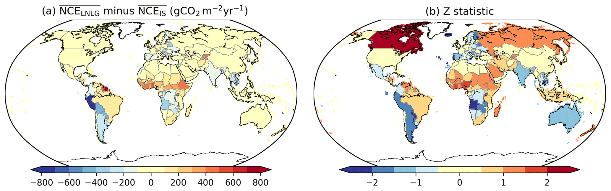
Figure 8Difference between LNLG and IS experiments. (a) minus and (b) the Z statistic (Eq. 7) indicating the difference between LNLG and IS experiments.
5.2 Fractional uncertainty reduction (FUR)
Byrne et al. (2022) report the uncertainty in NCE as the standard deviation across v10 OCO-2 MIP ensemble members (estimated using Eq. 4). This metric incorporates uncertainties related to model transport and aspects of the inversion configuration, such as optimization technique and a priori flux estimates. However, this metric is different to the uncertainty metric usually computed in a Bayesian framework, that is, the Bayesian posterior uncertainty. That uncertainty quantifies the impact of errors in the observations and prior constraints on the posterior flux estimates. The Bayesian posterior uncertainty is not reported for practical reasons, as the majority of contributing models do not calculate this quantity, so it is not possible to calculate this quantity across the ensemble.
In this section, we examine the posterior uncertainty estimates from two contributing inversion systems (CAMS and TM5-4DVar) and compare these estimates to the ensemble-based uncertainty estimate provided with the dataset. Then, we define the FUR metric between the posterior and prior NCE estimates based on the TM5-4DVar model (as CAMS does not estimate uncertainties for the LNLGIS and LNLGOGIS experiments), which can be used to understand the relative impact of assimilated atmospheric CO2 data on estimates of country-level NCE and ΔCloss.
Both CAMS and TM5-4DVar estimate CO2 fluxes using four-dimensional variational assimilation (4D-Var) and estimate posterior uncertainty estimates using a Monte Carlo method derived by Chevallier et al. (2007). The realism of the prior and posterior CAMS uncertainty estimates has already been the topic of several studies (see Chevallier, 2021, and references therein). Figure 9 shows the ensemble-based uncertainty, prior/posterior uncertainty from CAMS (prior, IS and LNLG only) and prior/posterior uncertainty from TM5-4DVar for four countries. Notably, the magnitudes of the prior/posterior uncertainties from CAMS and TM5-4DVar are quite different, with CAMS uncertainties being 2–8 times larger. Differences in prior/posterior uncertainties of this magnitude are not unusual among inversion systems and highlight the sensitivity of Bayesian uncertainty estimates to choices about prior uncertainties. Both CAMS and TM5-4DVar posterior uncertainties are smaller relative to their prior by similar fractions, driven by the assimilated CO2 data. The magnitude of the ensemble-based uncertainty tends to fall in between the CAMS and TM5-4DVar estimates. However, the CAMS and TM5-4DVar posterior uncertainty estimates decrease as more data are assimilated (as expected), while the ensemble spread does not. In fact, the ensemble spread increases with data density in some cases (e.g., Australia LNLGIS). Thus, overall, we find that the ensemble-based uncertainty estimate is of similar magnitude to the prior/posterior estimate but that the magnitude of posterior uncertainty is quite dependent on the assumed prior uncertainty.
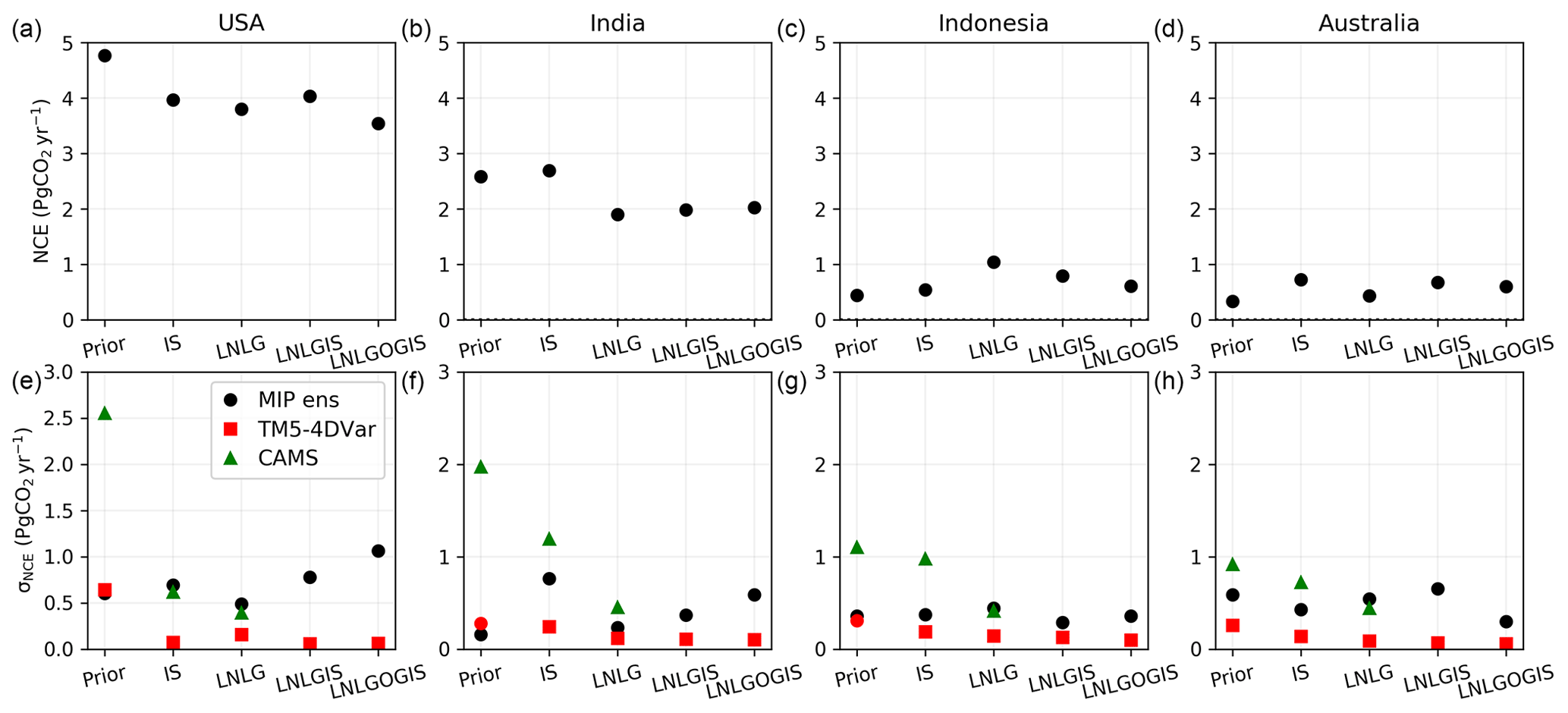
Figure 9(a–d) and (e–h) σNCE for four countries in 2018. The v10 OCO-2 MIP ensemble-spread-based error estimate is shown in black, the TM5-4DVar Bayesian uncertainty estimate is shown in red and the CAMS Bayesian uncertainty estimate is shown in green (only for Prior, IS and LNLG).
We now calculate the FUR metric in NCE from the TM5-4DVar Bayesian uncertainties (note that we use TM5-4DVar only because CAMS does not report LNLGIS or LNLGOGIS uncertainties). FUR is calculated from the prior flux standard deviation (σprior) and posterior flux standard deviation (σposterior) as
This quantity ranges between 0 and 1, with larger values indicating that the Bayesian uncertainties have decreased more (relative to the prior) due to the observational constraints from assimilated data. This metric is useful for understanding how the assimilation of data influences the NCE and ΔCloss estimates, which may not be captured by the ensemble spread. For example, Saudi Arabia has a small NCE uncertainty estimate, but this is largely driven by prior knowledge that biosphere CO2 fluxes, while the atmospheric CO2 data have little impact on the NCE estimate.
Figure 10 shows FUR for the IS, LNLG, LNLGIS and LNLGOGIS experiments. FUR is larger in regions with denser observational coverage. For example, the IS FUR is close to 1 in the USA and parts of Europe, reflecting dense CO2 measurements, but it remains small for many tropical countries, where sampling is sparse. Meanwhile, the LNLG experiment generally has larger FUR values than the IS experiment in the tropics, reflecting denser sampling, but has lower values for some small high-latitude countries, such as in Scandinavia.
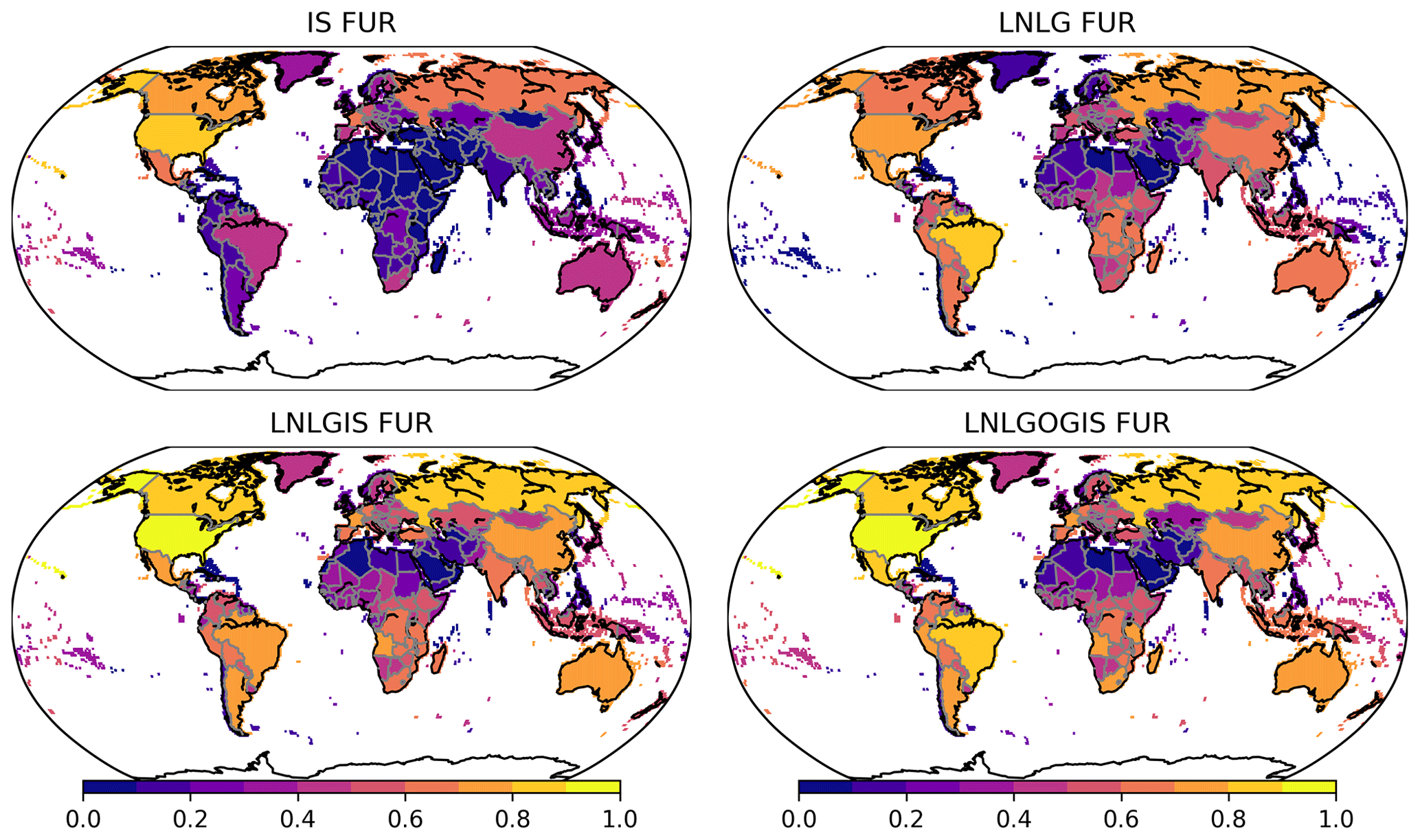
Figure 10Estimate of the fractional uncertainty reduction (FUR) on the v10 OCO-2 MIP estimates for each experiment based on Bayesian uncertainty estimates from the TM5-4DVar inversion.
The dataset described in this paper, Byrne et al. (2022), provides annual totals of country-level and 1∘ × 1∘ gridded ΔCloss, NBE, NCE, Frivers export and the combined Fcrop trade+Fwood trade fluxes, as well as their uncertainties over 2015–2020. In addition, the country-level Z statistic (Eq. 7) and FUR (Eq. 8) metrics are provided to help interpret the flux and stock change estimates. These data are provided for the v10 OCO-2 MIP IS, LNLG, LNLGIS and LNLGOGIS experiments. The OG experiment is excluded due to poor evaluation against independent CO2 measurements and pCO2-based air–sea fluxes, likely due to residual biases in the OCO-2 ocean glint retrievals (Sect. 4). We note that biases in ocean glint retrievals will also adversely impact flux estimates from the LNLGOGIS and caution against using these data when they show differences from the IS, LNLG and LNLGIS experiments. Future improvements to the OCO-2 retrievals are expected to reduce residual biases, and thus the quality of the LNLGOGIS experiment is expected to improve in future OCO-2 MIP experiments.
For the 1∘ × 1∘ gridded dataset, we emphasize that caution is needed in interpreting these data. As discussed in Sect. 1.3, atmospheric CO2 inversion analyses provide the best constraints on the largest spatial scales (e.g., continental-to-global). The confidence in these top-down estimates decreases at smaller spatial scales. The minimum spatial resolution for robust flux estimates is dependent on the density and precision of the measurements and is challenging to quantify. However, scales smaller than France or Germany in geographic extent are unlikely to be meaningfully constrained. Thus, we recommend only using 1∘ × 1∘ CO2 fluxes aggregated to larger spatial scales. In aggregating, we recommend propagating uncertainties by assuming first 100 % correlation (sum of the 1∘ × 1∘ uncertainties) and then 0 % correlation (square root of the sum of the squared uncertainties) between grid cells. We strongly encourage contacting the authors before using the gridded 1∘ × 1∘ dataset.
These data are available for download from the Committee on Earth Observation Satellites' (CEOS) website: https://doi.org/10.48588/npf6-sw92 (Byrne et al., 2022). The country-level data are available for download as comma-separated values (CSV), Network Common Data Form (NetCDF) and Microsoft Excel worksheet files. The 1∘ × 1∘ gridded dataset is available as a NetCDF file.
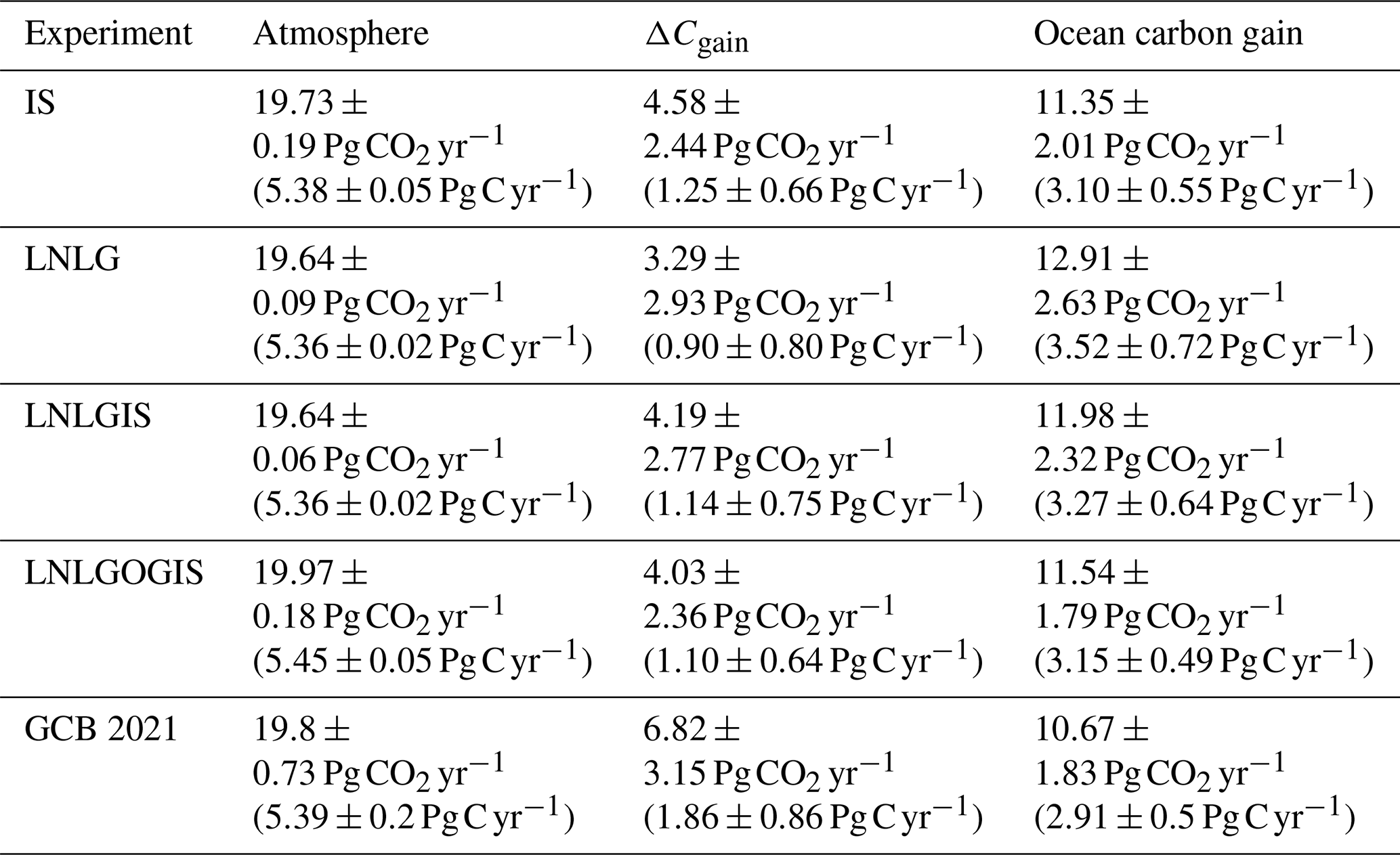
Globally, over 2015–2020, we report FF emissions of 35.79±1.50 Pg CO2 yr−1 (9.76±0.41 Pg C yr−1), Frivers export of Pg CO2 yr−1 ( Pg C yr−1), and globally balanced Fcrop trade and Fwood trade. Table 4 gives the global annual mean changes in the atmospheric burden of CO2, ΔCgain and ocean sequestration. Across the experiments, the median fraction of fossil fuel emissions remaining in the atmosphere is 55 %–56 %, while 32 %–36 % is sequestered by the ocean and 9 %–13 % is sequestered by terrestrial ecosystems. Note that this omits land-use change (LUC) emissions of ∼3.85 Pg CO2 yr−1 (∼1.05 Pg C yr−1, Friedlingstein et al., 2022), which are compensated for by additional carbon uptake by land. Of the combined FF+LUC emissions, 50 % remains in the atmosphere, 29 %–33 % is sequestered by the ocean and 18 %–21 % is sequestered by terrestrial ecosystems. Relative to the Global Carbon Budget 2021 (GCB 2021; Friedlingstein et al., 2022) we find 2.24–3.53 Pg CO2 yr−1 (0.61–0.96 Pg C yr−1) less removal by land (mean/median difference) but greater removal by the ocean of 0.87–2.24 Pg CO2 yr−1 (0.24–0.61 Pg C yr−1); however, these differences are consistent within 1 standard deviation of the mean/median values. Interestingly, we report greater removals by the ocean than GCB 2021 but reduced air–sea flux relative to SeaFlux. This can be explained by the fact that pCO2-based air–sea flux estimates generally give larger mean ocean carbon uptake than model estimates (Fay and McKinley, 2021) and that we estimate a larger Frivers export than GCB 2021.
Table 42015–2020 global mean atmospheric increase, terrestrial carbon gain (ΔCgain) and ocean carbon gain from the IS, LNLG, LNLGIS and LNLGOGIS experiments (mean/median ± 1 standard deviation). Positive values of ΔCgain and ocean carbon gain indicate increases in carbon stocks. GCB 2021 were obtained from the Global Carbon Budget 2021 (Friedlingstein et al., 2022) with ΔCgain calculated as the difference between the land sink and land-use change emissions with errors propagated in quadrature.
Meridionally, NCE is largest in the northern extratropics, coinciding with the largest FF emissions (Fig. 11). However, the northern extratropics also show negative ΔCloss, implying increasing terrestrial carbon stocks, particularly between 30–60∘ N. NCE is less positive in the tropics, primarily due to lower FF emissions. However, this region tends to show neutral-to-positive ΔCloss, suggesting that terrestrial carbon stocks may be decreasing. The LNLG and IS results also differ most in the tropics, with LNLG suggesting greater terrestrial carbon stock loss over 0–30∘ N but less over 0–30∘S. The differences in CO2 fluxes between these experiments are not well understood, and both experiments evaluate well against independent observations (Sect. 4).

Figure 11Zonal mean (a) NCE, (b) FF + lateral fluxes and (c) ΔCloss for 30∘ increments of latitude based on 1∘ × 1∘ estimates averaged over 2015–2020. IS, LNLG, LNLGIS and LNLGOGIS median estimates are shown by solid lines, and 1σ uncertainties are shown by the shaded region.
The spatial distribution of NCE over 2015–2020 at 1∘ × 1∘ and aggregated to country scale for the LNLGIS experiment is shown in Fig. 12. At 1∘ × 1∘ (Fig. 12a and b), localized fossil fuel emissions are visible, generally corresponding to urban areas and industrialized regions. These emissions are interspersed over broad source and sink structures that are driven by biosphere removals or emissions. Land biosphere removal is most evident across the northern mid-high latitudes. In contrast, tropical removals and emissions are more regional. When NCE is aggregated to the country scale (Fig. 12c and d), most countries are net sources driven by fossil fuel emissions, particularly in the northern extratropics. Figure 12e–f show the 2015–2020 mean country-level ΔCloss for the LNLGIS experiment. Increasing terrestrial carbon stocks (negative ΔCloss) are found for most extratropical countries, while tropical countries can have gains or losses. Notably, the uncertainty in ΔCloss is larger in the tropics, particularly for mid-sized countries. Overall, small to mid-sized countries generally have uncertainties comparable to the magnitude of ΔCloss, reflecting the fact that atmospheric CO2 measurements best constrain fluxes over large scales. Spatial maps of NCE and ΔCloss for each experiment are shown in the Supplement (Figs. S4–S7).
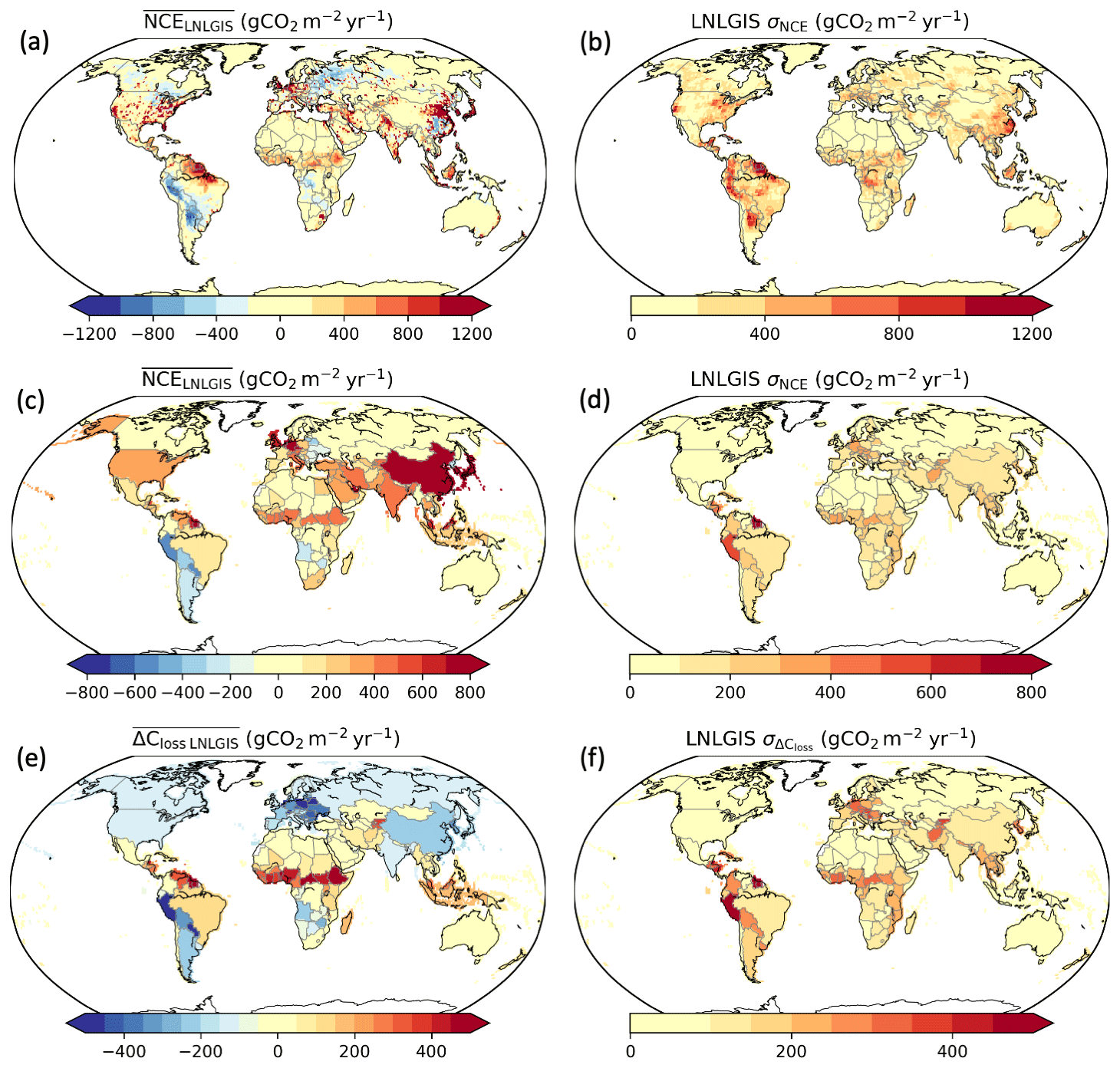
Figure 12Median () and 1 standard deviation (σNCE) of NCE on a (a, b) 1∘ × 1∘ grid and (c, d) aggregated to country scale for the v10 OCO-2 MIP LNLGIS experiment averaged over 2015–2020. (e, f) Median and 1 standard deviation of country-scale ΔCloss averaged over 2015–2020 derived from the LNLGIS v10 OCO-2 MIP experiment.
Differences in NCE and ΔCloss between the v10 OCO-2 MIP experiments can be considerable (the statistical significance of these differences is quantified by the Z statistic; see Sect. 5.1). The underlying cause of the differences between the v10 OCO-2 MIP experiments is not well understood, but the differences are likely impacted by the different spatial and temporal distribution of LNLG and IS measurements (see Sect. 5.2), model transport errors (Stephens et al., 2007; Schuh et al., 2019, 2022), and residual retrieval biases in the OCO-2 retrievals (Peiro et al., 2022). Unfortunately, the regions showing the largest differences in fluxes generally have few independent atmospheric CO2 measurements for validation, limiting our ability to distinguish between different causes. Thus, we believe that NCE and ΔCloss estimates are most reliable when agreement is found across the v10 OCO-2 MIP experiments.
We will now show examples of carbon budgets for four countries from this dataset. Figure 13 shows the 2015–2020 mean FF, Frivers export, Fcrop trade, Fwood trade, ΔCloss and NCE fluxes for the USA, India, Indonesia and Australia. All of the CO2 fluxes on the left of the dashed line combine to give the NCE flux constrained by the v10 OCO-2 MIP experiments. We find that FF is the strongest contributor to NCE for all countries but that ΔCloss also plays a strong modulating role. For example, negative ΔCloss (increasing terrestrial carbon stocks) for the USA reduces NCE to be less than would be expected given the FF emissions. Conversely, Indonesia has positive ΔCloss (decreasing terrestrial carbon stocks), resulting in increased NCE relative to FF. Some countries also show differences in ΔCloss between v10 OCO-2 MIP experiments. For example, the LNLG and LNLGIS experiments suggest negative ΔCloss for India, while the IS suggests ΔCloss is roughly neutral. Figures of carbon budgets for 28 additional countries (Fig. S8) and 14 regions (Fig. S9) are shown in the Supplement.

Figure 13CO2 budget for the USA, India, Indonesia and Australia averaged over 2015–2020. Bars show the median ± 1 standard deviation of FF, Frivers export (R), Fcrop trade+Fwood trade (CW), ΔCloss and NCE (note that these quantities are related through Eq. 2).
The carbon budgets can also be examined for individual years (Fig. 14). Both Indonesia and Australia show considerable variations in ΔCloss that drive variations in NCE over this period. Indonesia has a large positive ΔCloss in 2015, driven by warm, dry weather and fires during the 2015 El Niño (Yin et al., 2016). Australia showed strong negative ΔCloss (except for IS) during 2016, which was the 15th wettest year on record (precipitation 17 % above average; Bureau Of Meteorology, 2017). Australia also showed anomalous positive ΔCloss during 2019, which was the warmest and driest year on record, with considerable terrestrial carbon loss related to biomass burning in the southeast (Byrne et al., 2021). Variations in NCE are also found to be related to FF emissions. In particular, a reduction in NCE is found for 2019 and 2020 in the USA that is primarily linked to a reduction in FF emissions rather than ΔCloss. Time series of NCE and ΔCloss for 28 additional countries (Figs. S10, S11) and 14 regions (Figs. S12, S13) are shown in the Supplement.
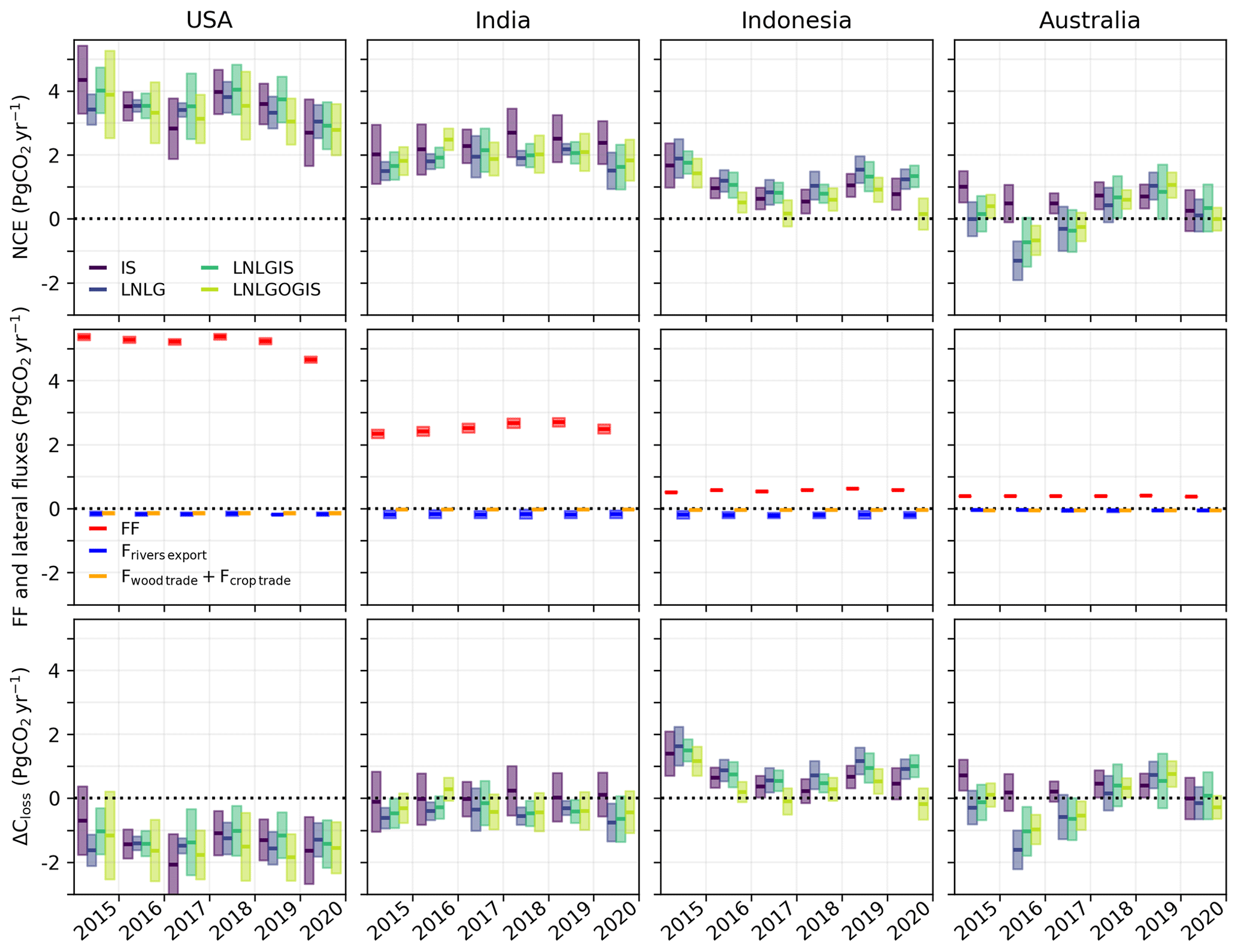
Figure 14Time series of the carbon budget for the USA, India, Indonesia and Australia. Solid lines show the median estimates, and shaded areas show ± 1 standard deviation.
We demonstrate how the dataset presented here can be compared with NGHGIs reported under the UNFCCC, which were downloaded from https://di.unfccc.int/flex_annex1 (last access: 6 February 2023). We also refer the reader to Chap. 6.10.2 in vol. 1 of IPCC (2019) for additional discussion of comparing top-down estimates with NGHGIs. The fossil fuel emissions in Byrne et al. (2022) can be compared with the combined emissions from the energy and IPPU (Energy+IPPU) categories. In both cases, these estimates account for anthropogenic CO2 emissions from the burning of fossil fuels and production of cement and other materials. We expect these estimates to generally be in good agreement, as they are similarly based on bottom-up accounting for national totals. However, the estimates may diverge when there are missing activity data, particularly in non-Annex 1 countries and more recent years (Andrew, 2020).
ΔCloss can be compared to the combined emissions and removals from the agriculture, LULUCF and waste (Agr+LULUCF+Waste) categories. These quantities are not identical, with the most important difference being that NGHGIs are only for managed land, while ΔCloss includes both managed and unmanaged lands. Therefore, caution is needed for parties with large unmanaged land areas (e.g., Canada or the Russian Federation). Another difference from NGHGIs is that ΔCloss implicitly includes deposition of carbon in water body sediments within a country (such as lakes). However, this is expected to be a small contribution. Similarly, volcanic CO2 emissions are implicitly included in ΔCloss but are also believed to be small contributions (global subaerial volcanic CO2 emissions are ∼0.05 Pg CO2 yr−1, Fischer et al., 2019). It is worth noting that NGHGIs require estimates of turnover times for wood products in producing countries, as these can have lifetimes of decades to centuries (see Appendix 3a.1 of Penman et al., 2003). No such estimate is needed for the top-down methods, as emissions from decaying wood products will be implicitly incorporated in NCE. Therefore, top-down methods only need to account for the lateral movement of wood products from the region where the carbon is sequestered to the region where the wood products are used and decompose.
For this analysis, we compare NGHGIs and our dataset for three entities: the USA, European Union plus the United Kingdom (EU27+UK) and Australia. These were chosen for two reasons. First, NCE is better constrained by atmospheric CO2 data over these relatively large regions. This is reflected in the FUR metric, which gives values of 0.76–0.91 for the USA (meaning a 76 %–91 % uncertainty reduction), 0.38–0.51 for EU27 and 0.45–0.78 for Australia. Second, each of these entities has small unmanaged land areas, making this more of an apples-to-apples comparison. An area of 95 % of the USA is managed, with most unmanaged land being in the state of Alaska (Ogle et al., 2018). Similarly, all land in the EU27+UK is considered managed except for 5 % of France's territory (Petrescu et al., 2021).
Figure 15 shows time series of emissions and removals from NGHGIs and Byrne et al. (2022) over 2015–2020. We focus our analysis on the 2015–2020 mean estimates, as top-down methods are expected to be more sensitive to IAV in the carbon cycle than NGHGI methods for individual years. Strong agreement is found between the NGHGI Energy+IPPU emissions and the fossil fuel emissions in Byrne et al. (2022), while larger differences are found between Agr+LULUCF+Waste and ΔCloss. Averaged over the 2015–2020 period, we obtain statistically significant differences between Agr+LULUCF+Waste and ΔCloss for the USA and EU27+UK for each experiment (based on Student's t test at 0.05 significance level). In each case the top-down estimates suggest greater carbon sequestration by land, with mean differences of 0.59–0.91 Pg CO2 yr−1 for the USA and 0.99–1.79 Pg CO2 yr−1 for the EU27+UK. The reasons for these differences are unclear but are not expected to be explained by removals in unmanaged lands. It is possible that NGHGI methods miss or underestimate sink processes and/or that there are biases affecting the top-down estimates (see Sect. 9 for remaining challenges in top-down estimates). We encourage further research and comparison between the NGHGI and top-down research communities to better understand the sources of these differences.

Figure 15Emissions and removals of CO2 from the (a–c) energy and IPPU categories and (d–f) agriculture, LULUCF and waste categories reported in NGHGIs and ΔCloss for four OCO-2 MIP experiments (IS, LNLG, LNLGIS, LNLGOGIS). Values are provided for individual years and the 2015–2020 mean.
Here we discuss the current limitations of top-down country-level CO2 budgets and activities that can improve these estimates. Section 9.1 discusses current CO2 observing systems and possible future expansions. Section 9.2 discusses current atmospheric CO2 inversion systems, planned developments and opportunities for improvement. Finally, Sect. 9.3 discusses remaining challenges in estimating carbon stock changes from atmospheric CO2 inversions.
9.1 Observations
In the context of global inversion analyses, annual mean biosphere–atmosphere CO2 fluxes are best informed by measurements of atmospheric CO2 on large spatial scales (e.g., continental-to-global) due to rapid mixing in the atmosphere and gaps in current measurement coverage. The confidence in these top-down estimates decreases as we move to smaller spatial scales, with the minimum spatial scale being dependent on the density, precision and sensitivity of the measurements. Future refinements in top-down CO2 budgets will depend on increasing observational density (Sect. 9.1.1), improved validation (Sect. 9.1.2) and data harmonization (Sect. 9.1.3).
9.1.1 Expanding observations
An expanding network of CO2 observing systems provides an opportunity to reduce uncertainties in top-down estimates of NCE. Across much of the globe, country-level estimates of NCE have been limited by the observational coverage of in situ CO2 measurements and retrievals. However, there are a number of planned expansions in observing systems that will help fill data gaps.
The first generation of space-based CO2 systems currently in operation (GOSAT, GOSAT-2, OCO-2, OCO-3, TanSat) were designed primarily as proof-of-concept missions to demonstrate that space-based measurements could yield retrievals with the precision and accuracy required to quantify emissions and removals of CO2. Planned future missions will expand and improve upon current observing systems. MicroCarb, a France–UK mission, is expected to start operations in 2023 with an additional spectral band to better characterize the light path for the estimation of (Bertaux et al., 2020). Japan's GOSAT-GW mission (https://gosat-gw.nies.go.jp/en/, last access: 6 February 2023), which will be launched in early 2025, will also incorporate improved capabilities for CO2 and CH4. In 2025, the European Copernicus program will begin to deploy the first operational CO2 and CH4 monitoring constellation, CO2M (Pinty et al., 2017; Janssens-Maenhout et al., 2020). The CO2M constellation will eventually include up to three satellites, flying in formation to collect measurements at 2 by 2 km resolution over the entire globe at weekly intervals. In addition, a follow-on to the Chinese TanSat mission is currently under development (Yang et al., 2018).
Most current and planned space-based CO2 observing systems are passive, in that they rely on reflected sunlight to retrieve . Active satellite missions, which use lidars for their light source, could provide coverage when reflected sunlight is not available or of insufficient intensity, such as at night and at high latitudes in the winter hemisphere when solar zenith angles are large. These systems also have the potential to better characterize systematic errors in current passive instruments by using pulse timing information to get a better estimate of path length and to filter out scattered light from clouds and aerosols (Abshire et al., 2010).
As space-based CO2 observing systems expand, sub-orbital discrete air sampling (i.e., flask) and continuous CO2 observing systems will remain critical for developing top-down CO2 budgets. These in situ observations are the global standard for GHG measurements, because they can undergo direct calibration relative to the World Meteorological Organization (WMO) CO2-in-air mole fraction scale, which is International System of Units (SI)-traceable (Hall et al., 2021). In contrast, open-path remote sensing measurements (both TCCON and satellite) can not be calibrated using standard gasses; they can only be compared to in situ vertical profile observations made relative to the WMO scale, with the differences used to adjust the remote sensing observations (e.g., Wunch et al., 2011). As such, in situ data are critical for linking remote sensing observations of CO2 to the accepted trace gas scales. In situ data also provide complementary observational coverage to space-based observing systems (Byrne et al., 2017). Space-based measurements have broad spatial coverage but with seasonal variations driven by sunlight and have data gaps in persistently cloudy regions. In contrast, flask and in situ data can be deployed year-round and regardless of cloud cover. Additionally, in situ observations most typically represent the planetary boundary layer where flux signals in atmospheric CO2 are larger than the signal as expressed in the column mean (Feng et al., 2019). Thus, these data play a critical role in improving carbon cycle constraints, especially in high-latitude and persistently cloudy regions (such as the tropics), and we encourage an expansion of these systems in these undersampled regions. Regular measurements of CO2 using light aircraft above several sites in Amazonia exist (e.g., Gatti et al., 2021; Miller et al., 2021), but these measurement records, as well as a nascent aircraft program in Uganda, have so far been funded using short-term grants.
Measurements of stable isotope () and radioisotope () ratios of carbon in CO2 provide powerful tools for source attribution. Radiocarbon is absent from fossil fuels, making it ideal for distinguishing fossil versus biologic carbon fluxes, and inversions using measurements of CO2 and have been used to provide top-down constraints on national-scale fossil CO2 emissions (Basu et al., 2020). Atmospheric ratios provide insight into ecosystem stress and its relation to climate via constraint of ecosystem water use efficiency (photosynthesis relative to water loss by transpiration) and have been used in box models (Keeling et al., 2017) and inversions (Peters et al., 2018). Atmospheric ratio data are generally available where discrete air samples are collected by various networks, but ratio data are more limited as they tend to require larger samples and measurement costs are greater. Other tracers closely related to CO2, such as (Keeling and Graven, 2021) and carbonyl sulfide (e.g., Hu et al., 2021; Remaud et al., 2022) are also limited yet provide valuable information on global ocean/NBE and regional-scale photosynthesis/respiration partitioning, respectively. Increasing the temporal and spatial density of these data, particularly across poorly sampled regions, will allow for more diagnostic power of carbon cycle processes than is possible with CO2 alone.
9.1.2 Data validation
Validation of retrievals is critical for ensuring that retrieval biases do not strongly impact flux estimates. Current gaps in coverage of ground-based and airborne measurements have limited our confidence in flux inferences from space-based data. For example, large CO2 emissions over northern sub-Saharan Africa are a robust feature of the inversions that assimilate satellite retrievals (Palmer et al., 2019), but there are few independent CO2 measurements to confirm whether this inference is a real signal or an artifact of regional retrieval biases. Increased validation of space-based observations will also provide critical support for improved space-based inferences. Space-based measurements rely on validation against ground-based retrievals from the TCCON (Wunch et al., 2011) and the COllaborative Carbon Column Observing Network (COCCON; Frey et al., 2019). In turn, these sites rely on in situ CO2 measurements from aircraft profiles and AirCore (Karion et al., 2010) to tie their measurements to the WMO scale (Wunch et al., 2010; Messerschmidt et al., 2011). These data have been critical for validating and improving retrievals (Wunch et al., 2017b; O'Dell et al., 2018; Kiel et al., 2019). Continued funding of these activities will be crucial for improving top-down CO2 flux estimates, and expansion of these observing systems into undersampled regions, such as the tropics and high latitudes, will also be important for identifying and addressing residual retrieval biases. In addition, efforts to cross-calibrate TCCON and COCCON sites will be helpful for minimizing site-to-site biases and identifying spurious drifts in . We encourage future campaigns aimed at site-to-site comparisons similar to the FRM4GHG campaign that deployed total column GHG traveling standard instruments at several TCCON sites as part of ESA's FRM4GHG-2 project (Sha et al., 2020).
9.1.3 Data harmonization
Further advancements in top-down flux estimates will be possible through combining the observational constraints from the constellation of space-based sensors and ground-based instruments. Assimilating these data concurrently within inversion systems will increase our ability to recover net fluxes over smaller regions. However, these instruments must be cross-calibrated against common standards to use these data together, as small intercalibration differences could potentially strongly impact flux estimates. We encourage support of these critical cross-calibration activities, as are outlined in Crisp et al. (2018).
9.2 Atmospheric CO2 inversions
Atmospheric CO2 inversion analyses are a critical tool for estimating surface fluxes from observations of atmospheric CO2. Expanding observational coverage provides both opportunities and challenges for inversion systems. By addressing the current limitations of our inversion systems, we will be able to take full advantage of increasing observations to improve country-level top-down estimates of NCE and ΔCloss. Here we discuss ongoing and planned developments (Sect. 9.2.1), improving model transport (Sect. 9.2.2), missing processes and required assumptions (Sect. 9.2.3), and uncertainty quantification (Sect. 9.2.4).
9.2.1 Ongoing and planned developments
To date, there are four operational or quasi-operational atmospheric CO2 inversion systems: CarbonTracker (Jacobson et al., 2020), CAMS (Chevallier et al., 2005b), Jena CarboScope (Rödenbeck et al., 2018) and CMS-Flux (J. Liu et al., 2021) that are regularly updated on annual or quarterly timescales. These systems produce NBE and air–sea flux estimates from either in situ CO2 measurements (CarbonTracker, Jena CarboScope), OCO-2 retrievals (CMS-Flux) or both (CAMS). Similarly, there are seven inversion models (including the aforementioned models) that update CO2 flux estimates annually for the Global Carbon Budget (Friedlingstein et al., 2022), including CAMS (Chevallier et al., 2005b), CarbonTracker Europe (CTE; Van der Laan-Luijkx et al., 2017), Jena CarboScope (Rödenbeck et al., 2018), UoE in situ (Feng et al., 2016), NISMON-CO2 (Niwa et al., 2017), MIROC4-ACTM (Saeki and Patra, 2017; Chandra et al., 2022) and CMS-Flux (J. Liu et al., 2021).
The OCO-2 MIP activities have semiregularly performed ensemble inversion experiments (Crowell et al., 2019; Peiro et al., 2022). To date, OCO-2 MIP experiments have been linked to new versions of the ACOS retrieval algorithm, with major improvements to the quality of retrievals occurring during each update. However, as the quality of retrievals have improved (particularly for ACOS v10 onwards), updates to the ACOS retrieval algorithm are becoming less of a driver for new OCO-2 MIP experiments. In the future, OCO-2 MIP activities could become more regular with annual updates.
The first top-down CO2 system for use in inventory development is CarbonWatch-NZ, under development in New Zealand (https://niwa.co.nz/climate/research-projects/carbon-watch-nz, last access: 6 February 2023). This program includes expanded CO2 measurement sites and the development of a regional atmospheric CO2 inverse system to quantify the carbon budgets of New Zealand's forest, grassland and urban environments. Initial results suggest stronger uptake by intact forests than estimated through bottom-up estimates (Steinkamp et al., 2017). This system may serve as an example for other nations through the Integrated Global GHG Information System (IG3IS) framework.
Beyond existing activities, there are a number of planned projects. The European Commission's Copernicus program (https://www.copernicus.eu, last access: 6 February 2023) has a number of developments ongoing and planned, particularly in building anthropogenic CO2 emission monitoring and verification support capacity (CO2MVS; Janssens-Maenhout et al., 2020), which is directly linked to the development and launch of the new CO2M mission and is expected to be operational from 2026 onwards. Further, there are a number of recently completed, ongoing and planned projects to develop and improve inversion systems to develop operational capacity. Examples include the recently completed CO2 Human Emissions (CHE) project (https://www.che-project.eu/, last access: 6 February 2023) and the follow-up CoCO2 project (https://coco2-project.eu/, last access: 6 February 2023) that is ongoing, as well as the VERIFY project (https://verify.lsce.ipsl.fr/, last access: 6 February 2023). These projects are developing and refining inversion systems to estimate anthropogenic fossil fuel emissions, as well as emissions and removals from the agriculture, LULUCF and waste categories. Future planned projects include developing approaches to utilize co-emitted species and auxiliary observations (14C, solar-induced fluorescence, carbonyl sulfide and others) in order to isolate some of the CO2 budget components and improve our understanding of the carbon cycle. For example, multiple data streams could be used together to optimize the dynamic global vegetation model parameters (e.g., Peylin et al., 2016).
In contrast to recent European efforts, there is no mandate for an operational top-down carbon-flux-attribution system in the USA. Nevertheless, efforts at NOAA centered around CarbonTracker (Jacobson et al., 2020) have been able to produce NBE estimates with relatively low latency, harnessing the agency's substantial flask and in situ CO2 network. In addition, NOAA has developed a higher-spatial-resolution North American regional inverse system, CarbonTracker-Lagrange (https://gml.noaa.gov/ccgg/carbontracker-lagrange/, last access: 6 February 2023; Hu et al., 2019). In anticipation of the launch of OCO in 2009, NASA started supporting research and development efforts needed to prototype an operational flux estimation system. In particular, the Carbon Monitoring System program (https://carbon.nasa.gov/, last access: 6 February 2023) has led to the development of both low-latency (2 months) atmospheric CO2 reanalysis (Weir et al., 2021a) and approaches to combine top-down NCE estimates with other trace gas measurements (e.g., CO) and non-atmospheric carbon data (e.g., above-ground biomass) to provide improved understanding of carbon cycle processes (Liu et al., 2017; Byrne et al., 2020, 2021; Bloom et al., 2020). There is substantial technical capacity to build an operational system, but this requires a coordinated effort between federal agencies, academia and private interests.
In Canada, a prototype operational regional inverse modeling system, the Environment and Climate Change Canada (ECCC) National Carbon Flux Inversion System (ENCIS), is being developed to provide quantitative information on CO2 (and CH4) flux estimates over Canada from national to provincial scales, as well as to understand the carbon cycle in Canada such as CO2 flux in boreal managed and unmanaged forests, wetland emissions of CH4, and GHG emissions over a potentially thawing permafrost in response to the climate change. ENCIS is a regional inverse modeling system based on a Lagrangian approach and driven by metrology from the Global Environmental Multiscale (GEM) model (Girard et al., 2014) and is expected to have 1∘ × 1∘ spatial resolution.
Finally, there are ongoing internationally organized activities. Phase 2 of the Regional Carbon Cycle Assessment and Processes project (RECCAP-2), coordinated by the Global Carbon Project (https://www.globalcarbonproject.org/reccap/, last access: 6 February 2023), has aimed to characterize regional carbon budgets. This included investigating how different data sources – including atmospheric inversion analyses – can contribute to this goal (Bastos et al., 2022; Deng et al., 2022). In addition, the WMO has hosted workshops and symposiums with the GHG monitoring community to develop a framework for sustained, internationally coordinated global GHG monitoring (e.g., https://community.wmo.int/meetings/wmo-international-greenhouse-gas-monitoring-symposium, last access: 6 February 2023).
9.2.2 Improving CTM transport
Errors in the representation of atmospheric transport by CTMs have long been recognized as a major source of error in atmosphere CO2 inversion analyses (Law et al., 1996; Law and Simmonds, 1996; Denning et al., 1995, 1999a, b; D. Baker et al., 2006; Stephens et al., 2007). Improvements to model transport will provide critical improvements to NCE and ΔCloss estimates. Systematic errors in model transport limit our ability to relate surface fluxes and CO2 observations and can lead to incorrect inferences of surface fluxes (Yu et al., 2018; Schuh et al., 2019; Stanevich et al., 2020). Improving model transport will require work in two areas: (1) improving model parameterizations of unresolved transport, particularly in coarse offline CTMs (like GEOS-Chem run at 4∘ × 5∘ in this ensemble) where the spatial and temporal coarsening of meteorological fields can “average out” vertical transport that is resolved in the parent model (Yu et al., 2018; Stanevich et al., 2020); and (2) increasing spatial and temporal resolution in model simulations, which can better resolve atmospheric transport processes (Agustí-Panareda et al., 2019; Schuh et al., 2019). However, it should be noted that there are limitations to the improvements that can come from increased model resolution in the global inversion context due to underlying meteorological uncertainties (Liu et al., 2011; Polavarapu et al., 2016, 2018; McNorton et al., 2020). Computational cost is also a significant challenge in inversion systems, because transport models usually scale poorly on supercomputers, for example because of the volume of meteorological data required as input.
As transport models are refined, it will be critical to periodically test their ability to represent large-scale atmospheric dynamics. This can be tested using long-lived trace gas species, including sulfur hexafluoride (Schuh et al., 2019), idealized age of air tracer (Krol et al., 2018) and beryllium-7 (Stanevich et al., 2020). Simulations of these trace species are critical in the context of inversion MIPs to gauge intermodel variability and average model bias (Schuh et al., 2019). Similarly, 222Rn is a useful short-lived gas species that enables modelers to evaluate the vertical mixing within the column (Remaud et al., 2018). In addition, model intercomparison studies have proven useful for diagnosing transport errors (e.g., Gaubert et al., 2019; Zhang et al., 2022), and we recommend further activities, such as within the Atmospheric Tracer Transport Model Intercomparison Project (TRANSCOM) framework.
9.2.3 Missing processes and required assumptions
The flux estimates provided here do not explicitly account for the atmospheric chemical production of atmospheric CO2, which occurs from the oxidation of reduced carbon gasses. Instead, these fluxes are either prescribed as surface–atmosphere fluxes (e.g., for FF CO emissions) or neglected from the prior fluxes. This can cause inverse modeling systems to implicitly incorporate the atmospheric CO2 source in optimized surface–atmosphere emissions and removals (i.e., air–sea fluxes and NBE), which can be far from the actual source of the reduced gas. For example, FF CO emissions are largely emitted in the northern extratropics but largely oxidized to CO2 in the tropical troposphere. These incorrectly located emissions of CO2 are large enough to impact top-down inversions (Enting and Mansbridge, 1991; Suntharalingam et al., 2005; Nassar et al., 2010; Wang et al., 2020). Future studies that aim to incorporate an atmospheric source of CO2 would help correct for this current spatial bias (Ciais et al., 2022).
A critical assumption in the top-down CO2 budgets estimated here has been that FF emissions are known and unbiased. Uncertainties in inventory-based FF emission estimates at global and country levels (e.g., Andres et al., 2014) are smaller than top-down NCE estimates; however, inventory-based emission estimates are prone to systematic biases due to the nature of the estimation approach (Guan et al., 2012; Oda et al., 2019), and FF uncertainties could bias the partitioning of NCE between FF and NBE (and propagate into ΔCloss) over countries with large emissions and lower reliability of statistical data collection systems, such as China. For example, Saeki and Patra (2017) show that an inferred increase in removals of CO2 by the biosphere over China during 2001–2010 is likely to be an artifact imposed by an error in the trend of anthropogenic CO2 emissions.
9.2.4 Uncertainty quantification
The uncertainty in NCE reported here is an estimate of the standard deviation of the v10 OCO-2 MIP ensemble members. This is meant to characterize uncertainties originating from the inversion configuration (such as the transport model, inversion method and prior constraints). However, there are also limitations to this method. First, there is only a small ensemble of 11 MIP ensemble members included in this analysis and an over-representation of inversions using two transport models: TM5 (3) and GEOS-Chem (5), which makes uncertainty quantification challenging. Future approaches that employ “borrowing strength” (Mearns and et al., 2007; Cressie and Kang, 2016) could be employed to better characterize ensemble uncertainty. Second, the ensemble-based estimate does not capture some sources of uncertainty. In particular, Bayesian posterior uncertainties are not considered here (see Sect. 5.2), due to the fact that many of the inversion systems participating in the v10 OCO-2 MIP do not calculate this uncertainty. In addition, we find that the ensemble members that produce Bayesian uncertainties show large differences in magnitude. Thus, this is an area of future improvement for MIP activities, and we recommend more work into characterizing this error component in ensemble inversion experiments. We also note that using an analytic framework, posterior uncertainties and their sensitivities to prior information could be further examined, as has been done for methane (Worden et al., 2022).
9.3 Stock change estimates
Agriculture and LULUCF emissions and removals are generally quantified as terrestrial carbon stock changes in managed lands. A number of challenges remain in estimating this quantity from top-down methods. Firstly, lateral fluxes of carbon remain quite uncertain (and associated uncertainty estimates are themselves quite uncertain). The best constrained lateral fluxes are annual country-level Fwood trade and Fwood trade, which are reported to the UN Food and Agriculture Organization. These fluxes are more uncertain on sub-national scales and sub-annual timescales. Meanwhile, Frivers export is best quantified on basin scales, where stream gauge measurements inform carbon fluxes. Improving sub-national and sub-annual estimates of lateral fluxes would have several benefits: first, this would allow for better sub-national attribution, where regional fluxes could be better quantified. Second, this would allow for incorporating the atmospheric imprint of these carbon fluxes as prior information within atmospheric CO2 inversion analyses, which may improve flux estimates on sub-national scales.
The GST and Paris Agreement do not consider emissions and removals from unmanaged lands. Separating managed lands from unmanaged lands remains a major challenge, given the smoothed large-scale CO2 flux constraints provided by these top-down methods and the fact that both managed and unmanaged lands can experience considerable stock changes driven by interannual climate variations (e.g., El Niño) and in response to rising CO2 and climate change. In addition, separating managed and unmanaged lands is further complicated by the fact that there is considerable ambiguity in the definitions of managed lands, which can also vary by country (Grassi et al., 2018; Chevallier, 2021). We recommend that each party provide a mask to unambiguously define the plots considered managed from year to year (Chevallier, 2021).
Top-down CO2 budgets are available from the Committee on Earth Observation Satellites' (CEOS) website: https://doi.org/10.48588/npf6-sw92 (Byrne et al., 2022). Gridded NBE and air–sea fluxes from the OCO-2 MIP are available at https://gml.noaa.gov/ccgg/OCO2_v10mip/ (Baker et al., 2023). Fossil fuel emissions prescribed in the inversions can be downloaded from https://doi.org/10.5281/zenodo.4776925 (Basu and Nassar, 2021). The ODIAC2020 emission data product can be downloaded from the Global Environmental Database hosted by the Center for Global Environmental Research at NIES (https://doi.org/10.17595/20170411.001, Oda and Maksyutov, 2015). SeaFlux pCO2-based air–sea fluxes were downloaded from https://doi.org/10.5281/zenodo.5482547, (Gregor and Fay, 2021b).
We introduced a pilot top-down CO2 budget dataset (Byrne et al., 2022) intended to start a dialogue between research communities and to identify ways that top-down flux estimates can inform country-level carbon budgets. This dataset provides annual country-level and 1∘ × 1∘ gridded top-down NCE and ΔCloss over 2015–2020, in addition to bottom-up FF and lateral fluxes. These data are provided for four experiments from the v10 OCO-2 MIP that differ in the data used in the assimilation: IS, LNLG, LNLGIS and LNLGOGIS. In addition, we provide two metrics for interpreting country-level estimates: (1) the Z statistic (Sect. 5.1), which quantifies the agreement between IS and LNLG NCE estimates, and (2) the FUR (Sect. 5.2), which quantifies the impact of atmospheric CO2 data in reducing flux uncertainties.
Country-level flux estimates generally show robust signals for large extratropical countries (e.g., USA, Russia, China). Agreement between the experiments generally decreases for mid-sized countries (e.g., Turkey), particularly in regions with sparse observational coverage for the in situ network (such as the tropics). Large divergences between the IS and LNLG experiments occur in some regions, particularly in northern sub-Saharan Africa, and could be related to the sparsity of in situ CO2 measurements or biases in OCO-2 retrievals. However, the sparsity of independent CO2 measurements in these regions precludes definitive conclusions. We urge caution in interpreting the 1∘ × 1∘ gridded results and suggest collaborating with experts in atmospheric CO2 inversion systems when using those data.
The accuracy of top-down NCE estimates was characterized through comparisons against independent atmospheric CO2 datasets and through comparisons against pCO2-based air–sea CO2 fluxes. Overall, the IS, LNLG and LNLGIS were found to show the best agreement against independent CO2 measurements, and we recommend using these experiments for analysis. Poorer agreement was found for experiments assimilating OCO-2 ocean glint retrievals, suggesting that residual retrieval biases adversely impact the LNLGOGIS experiment, and we urge caution in interpreting these data.
For future GSTs, top-down NCE estimates will be refined as new space-based observing systems expand and retrieval algorithms are improved. Complementary expansions of ground-based and aircraft-based CO2 measurements in undersampled regions will similarly fill critical observational gaps in regions with large uncertainties and susceptibility to retrieval biases. Improvements to atmospheric CO2 inversion systems, including reductions to systematic transport errors and improved error characterization, will be critical for refining top-down CO2 budgets. And improved estimates of lateral carbon fluxes and managed land maps will refine estimates of agriculture, LULUCF, and waste emissions and removals.
Table A1TCCON sites used for evaluation of posterior CO2 fields of the v10 OCO-2 MIP experiments.
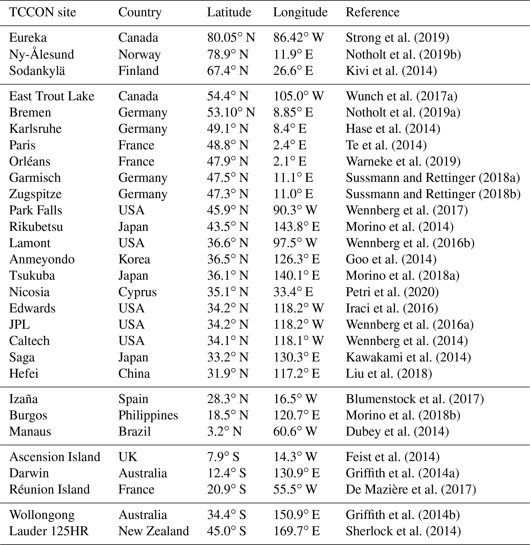
The supplement related to this article is available online at: https://doi.org/10.5194/essd-15-963-2023-supplement.
The study was conceived of by DCr and designed by BB, DFB, SB, KWB, AC, FC, PC, NC, DCr, SF, LH, ARJ, JL, JBM, TO, PKP, BP, AS, CS and JRW. The v10 OCO-2 MIP experiments were performed by DFB, SB, MB, FC, NC, SC, FD, ARJ, RJ, MSJ, DBAJ, JL, ZL, SM, SMM, MR, AS, AZM and NZ. Lateral flux estimates were performed by FC, PC, ZD, HT and YY. FF emission estimates were performed by TO and SB. TCCON data were collected by NMD, MKD, OEG, BH, RK, IM, JN, YSO, HO, CP, KS, KS, YT, VAV, MV, TW and DW. Evaluation of v10 OCO-2 MIP against co-samples was performed by BB, SB, AC and ARJ. BB wrote the paper and prepared the figures, with contributions from all co-authors.
At least one of the (co-)authors is a member of the editorial board of Earth System Science Data. The peer-review process was guided by an independent editor, and the authors also have no other competing interests to declare.
Publisher's note: Copernicus Publications remains neutral with regard to jurisdictional claims in published maps and institutional affiliations.
Part of this research was carried out at the Jet Propulsion Laboratory, California Institute of Technology, under a contract with the National Aeronautics and Space Administration (grant no. 80NM0018D004). The v10 OCO-2 MIP activity was supported by the NASA OCO science team program. Brendan Byrne and Junjie Liu were supported by the NASA OCO-2 and OCO-3 science team program (grant no. NNH17ZDA001N-OCO2). Andrew R. Jacobson, Andrew Schuh and David F. Baker were funded by NASA (grant no. 80NSSC21K1080). Andrew Schuh was also supported by NASA (grant no. NNX15AG93G). Sean Crowell acknowledges support from the NASA OCO science team (grant no. 80NSSC21K1077). The research of Noel Cressie, Andrew Zammit-Mangion, and Michael Bertolacci was supported by the Australian Research Council Discovery Project (grant no. DP190100180) and by NASA ROSES (grant no. 20-OCOST20-0004). Andrew Zammit-Mangion is also supported by the Australian Research Council Discovery Early Career Research Award (grant no. DE180100203). The contribution of Abhishek Chatterjee was supported by NASA ROSES (grant nos. 80NSSC20K0006 and 80NSSC21K1068). Matthew S. Johnson acknowledges the internal funding from NASA's Earth Science Research and Analysis Program. The contributions of Frédéric Chevallier and Marine Remaud were supported by the Copernicus Atmosphere Monitoring Service and implemented by the European Centre for Medium-Range Weather Forecasts on behalf of the European Commission (grant no. CAMS73) and by the European Union's Horizon 2020 Research and Innovation Programme under grant agreement number 958927 (prototype system for a Copernicus CO2 service). It was granted access to the HPC resources of TGCC under the allocation A0110102201 made by GENCI. Sha Feng at PNNL is supported by the NASA Carbon Monitoring Program (grant no. 80HQTR21T0069). The Pacific Northwest National Laboratory is operated by Battelle Memorial Institute under contract DE-AC05-76RL01830. Ning Zeng acknowledges support from NOAA (grant no. NA18OAR4310266) and NASA (grant no. 80NSSC18K0908). Prabir K. Patra is partly supported by the Environment Research and Technology Development Fund (grant no. JPMEERF21S20800) of the Environmental Restoration and Conservation Agency of Japan. Scot M. Miller was supported by the NASA grants 80NSSC18K0976 and 80NSSC21K1073. Nicholas M. Deutscher was funded by the ARC Future Fellowship (grant no. FT180100327).
The TCCON Nicosia site has received additional support from the European Union's Horizon 2020 Research and Innovation Programme (grant no. 856612/EMME-CARE), the Cyprus Government and the University of Bremen. The TCCON Anmyeondo site has been funded by the Korea Meteorological Administration Research and Development Program, Developing Technology for Integrated Climate Change Monitoring and Analysis, under grant KMA2018-00320. TCCON sites at Tsukuba, Rikubetsu and Burgos are supported in part by the GOSAT series project. Burgos is supported in part by the Energy Development Corp., Philippines. The Eureka TCCON measurements were made at the Polar Environment Atmospheric Research Laboratory (PEARL) by the Canadian Network for the Detection of Atmospheric Change (CANDAC), primarily supported by the Natural Sciences and Engineering Research Council of Canada, Environment and Climate Change Canada, and the Canadian Space Agency. The TCCON site at Réunion Island has been operated by the Royal Belgian Institute for Space Aeronomy with financial support since 2014 by the EU project ICOS-Inwire and the ministerial decree for ICOS (FR/35/IC1 to FR/35/C6) and local activities supported by LACy/UMR8105 and by OSU-R/UMS3365 – Université de La Réunion. Darwin and Wollongong TCCON stations are supported by ARC grants DP160100598, LE0668470, DP140101552, DP110103118 and DP0879468 and NASA grants NAG512247 and NNG05GD07G.
We thank Robert J. Andres for providing uncertainty estimates for CDIAC fossil fuel emission estimates. We thank the data providers of the SeaFlux ensemble for making their pCO2-based air–sea CO2 fluxes publicly available. We are grateful for the leadership of Annemarie Eldering and Mike Gunson of the OCO-2 mission, whose hard work has made this dataset possible.
This research has been supported by the European Commission, Horizon 2020 Framework Programme (CoCO2 (grant no. 958927 856612/EMME-CARE)) and Copernicus Atmosphere Monitoring Service (grant no. CAMS73), the Australian Research Council (grant nos. DP190100180, DE180100203, DP160100598, LE0668470, DP140101552, DP110103118, DP0879468 and FT180100327), the Environmental Restoration and Conservation Agency (grant no. JPMEERF21S20800), the Korea Meteorological Administration (grant no. KMA2018-00320), the National Aeronautics and Space Administration (grant nos. 20-OCOST20-0004, 80NSSC18K0908, 80NSSC18K0976, 80NSSC20K0006, 80NSSC21K1068, 80NSSC21K1073, 80NSSC21K1077, 80NSSC21K1080, 80HQTR21T0069, NAG512247, NNG05GD07G, NNH17ZDA001N-OCO2 and NNX15AG93G), and the National Oceanic and Atmospheric Administration (grant no. NA18OAR4310266).
This paper was edited by David Carlson and reviewed by two anonymous referees.
Abshire, J. B., Riris, H., Allan, G. R., Weaver, C. J., Mao, J., Sun, X., Hasselbrack, W. E., Kawa, S. R., and Biraud, S.: Pulsed airborne lidar measurements of atmospheric CO2 column absorption, Tellus B, 62, 770–783, https://doi.org/10.1111/j.1600-0889.2010.00502.x, 2010. a
Agustí-Panareda, A., Diamantakis, M., Massart, S., Chevallier, F., Muñoz-Sabater, J., Barré, J., Curcoll, R., Engelen, R., Langerock, B., Law, R. M., Loh, Z., Morguí, J. A., Parrington, M., Peuch, V.-H., Ramonet, M., Roehl, C., Vermeulen, A. T., Warneke, T., and Wunch, D.: Modelling CO2 weather – why horizontal resolution matters, Atmos. Chem. Phys., 19, 7347–7376, https://doi.org/10.5194/acp-19-7347-2019, 2019. a
Anav, A., Friedlingstein, P., Beer, C., Ciais, P., Harper, A., Jones, C., Murray-Tortarolo, G., Papale, D., Parazoo, N. C., Peylin, P., Piao, S., Sitch, S., Nicolas, V., Andy, W., and Zhao, M.: Spatiotemporal patterns of terrestrial gross primary production: A review, Rev. Geophys., 53, 785–818, https://doi.org/10.1002/2015RG000483, 2015. a
Andres, R. J., Boden, T. A., and Higdon, D.: A new evaluation of the uncertainty associated with CDIAC estimates of fossil fuel carbon dioxide emission, Tellus B, 66, 23616, https://doi.org/10.3402/tellusb.v66.23616, 2014. a, b, c
Andrew, R. M.: A comparison of estimates of global carbon dioxide emissions from fossil carbon sources, Earth Syst. Sci. Data, 12, 1437–1465, https://doi.org/10.5194/essd-12-1437-2020, 2020. a
Baier, B., Sweeney, C., Tans, P., Newberger, T., Higgs, J., and Wolter, S.: NOAA AirCore atmospheric sampling system profiles (Version 20210813), NOAA Global Monitoring Laboratory [data set], https://doi.org/10.15138/6AV0-MY81, 2021. a
Baker, D., Law, R. M., Gurney, K. R., Rayner, P., Peylin, P., Denning, A., Bousquet, P., Bruhwiler, L., Chen, Y.-H., Ciais, P., Fung, I. Y., Heimann, M., John, J., Maki, T., Maksyutov, S., Masarie, K., Prather, M., Pak, B., Taguchi, S., and Zhu, Z.: TransCom 3 inversion intercomparison: Impact of transport model errors on the interannual variability of regional CO2 fluxes, 1988–2003, Global Biogeochem. Cy., 20, GB1002, https://doi.org/10.1029/2004GB002439, 2006. a
Baker, D. F., Bösch, H., Doney, S. C., O'Brien, D., and Schimel, D. S.: Carbon source/sink information provided by column CO2 measurements from the Orbiting Carbon Observatory, Atmos. Chem. Phys., 10, 4145–4165, https://doi.org/10.5194/acp-10-4145-2010, 2010. a
Baker, D. F., Doney, S. C., and Schimel, D. S.: Variational data assimilation for atmospheric CO2, Tellus B, 58, 359–365, 2006. a
Baker, D. F., Bell, E., Davis, K. J., Campbell, J. F., Lin, B., and Dobler, J.: A new exponentially decaying error correlation model for assimilating OCO-2 column-average CO2 data using a length scale computed from airborne lidar measurements, Geosci. Model Dev., 15, 649–668, https://doi.org/10.5194/gmd-15-649-2022, 2022. a
Baker, D. F., Basu, S., Bertolacci, M., Chevallier, F., Cressie, N., Crowell, S., Deng, F., He, W., Jacobson, A. R., Janardanan, R., Jiang, F., Johnson, M. S., Jones, D. B. A., Liu, J., Liu, Z., Maksyutov, S., Miller, S. M., Philip, S., Schuh, A., Weir, B., Zammit-Mangion, A., and Zeng, N.: v10 Orbiting Carbon Observatory-2 model intercomparison project, NOAA Global Monitoring Laboratory [data set], https://gml.noaa.gov/ccgg/OCO2_v10mip/, last access: 6 February 2023. a
Ballantyne, A. P., Alden, C. B., Miller, J. B., Tans, P. P., and White, J.: Increase in observed net carbon dioxide uptake by land and oceans during the past 50 years, Nature, 488, 70–72, https://doi.org/10.1038/nature11299, 2012. a
Bastos, A., Ciais, P., Sitch, S., Aragão, L. E., Chevallier, F., Fawcett, D., Rosan, T. M., Saunois, M., Günther, D., Perugini, L., Robert, C., Deng, Z., Pongratz, J., Ganzenmüller, R., Fuchs, R., Winkler, K., Zaehle, S., and Albergel, C. : On the use of Earth Observation to support estimates of national greenhouse gas emissions and sinks for the Global stocktake process: lessons learned from ESA-CCI RECCAP2, Carbon balance and management, 17, 1–16, 2022. a
Basu, S. and Nassar, R.: Fossil Fuel CO2 Emissions for the OCO2 Model Intercomparison Project (MIP) (2020.1), Zenodo [data set], https://doi.org/10.5281/zenodo.4776925, 2021. a
Basu, S., Lehman, S. J., Miller, J. B., Andrews, A. E., Sweeney, C., Gurney, K. R., Xu, X., Southon, J., and Tans, P. P.: Estimating US fossil fuel CO2 emissions from measurements of 14C in atmospheric CO2, P. Natl. Acad. Sci. USA, 117, 13300–13307, https://doi.org/10.1073/pnas.1919032117, 2020. a
Bertaux, J.-L., Hauchecorne, A., Lefèvre, F., Bréon, F.-M., Blanot, L., Jouglet, D., Lafrique, P., and Akaev, P.: The use of the 1.27 µm O2 absorption band for greenhouse gas monitoring from space and application to MicroCarb, Atmos. Meas. Tech., 13, 3329–3374, https://doi.org/10.5194/amt-13-3329-2020, 2020. a
Bloom, A. A., Bowman, K. W., Liu, J., Konings, A. G., Worden, J. R., Parazoo, N. C., Meyer, V., Reager, J. T., Worden, H. M., Jiang, Z., Quetin, G. R., Smallman, T. L., Exbrayat, J.-F., Yin, Y., Saatchi, S. S., Williams, M., and Schimel, D. S.: Lagged effects regulate the inter-annual variability of the tropical carbon balance, Biogeosciences, 17, 6393–6422, https://doi.org/10.5194/bg-17-6393-2020, 2020. a
Blumenstock, T., Hase, F., Schneider, M., García, O. E., and Sepúlveda, E.: TCCON data from Izana (ES), Release GGG2014.R1, https://doi.org/10.14291/TCCON.GGG2014.IZANA01.R1, 2017. a
Bolin, B. and Keeling, C.: Large-scale atmospheric mixing as deduced from the seasonal and meridional variations of carbon dioxide, J. Geophys. Res., 68, 3899–3920, https://doi.org/10.1029/JZ068i013p03899, 1963. a
Bureau Of Meteorology: Annual climate statement 2016, http://www.bom.gov.au/climate/current/annual/aus/2016 (last access: 10 June 2022), 2017. a
Byrne, B., Jones, D. B. A., Strong, K., Zeng, Z.-C., Deng, F., and Liu, J.: Sensitivity of CO2 Surface Flux Constraints to Observational Coverage, J. Geophys. Res.-Atmos, 112, 6672–6694, https://doi.org/10.1002/2016JD026164, 2017. a
Byrne, B., Liu, J., Bloom, A. A., Bowman, K. W., Butterfield, Z., Joiner, J., Keenan, T. F., Keppel-Aleks, G., Parazoo, N. C., and Yin, Y.: Contrasting regional carbon cycle responses to seasonal climate anomalies across the east-west divide of temperate North America, Global Biogeochem. Cy., 34, e2020GB006598, https://doi.org/10.1029/2020GB006598, 2020. a
Byrne, B., Liu, J., Lee, M., Yin, Y., Bowman, K. W., Miyazaki, K., Norton, A. J., Joiner, J., Pollard, D. F., Griffith, D. W., Velazco, V. A., Deutscher, N. M., Jones, N. B., and Paton-Walsh, C.: The carbon cycle of southeast Australia during 2019–2020: Drought, fires, and subsequent recovery, AGU Adv., 2, e2021AV000469, https://doi.org/10.1029/2021AV000469, 2021. a, b
Byrne, B., Baker, D. F., Basu, S., Bertolacci, M., Bowman, K. W., Carroll, D., Chatterjee, A., Chevallier, F., Ciais, P., Cressie, N., Crisp, D., Crowell, S., Deng, F., Deng, Z., Deutscher, N. M., Dubey, M. K., Feng, S., García, O. E., Herkommer, B., Hu, L., Jacobson, A. R., Janardanan, R., Jeong, S., Johnson, M. S., Jones, D. B. A., Kivi, R., Liu, J., Liu, Z., Maksyutov, S., Miller, J. B., Miller, S. M., Morino, I., Notholt, J., Oda, T., O'Dell, C. W., Oh, Y.-S., Ohyama, H., Patra, P. K., Peiro, H., Petri, C., Philip, S., Pollard, D. F., Poulter, B., Remaud, M., Schuh, A., Sha, M. K., Shiomi, K., Strong, K., Sweeney, C., Té, Y., Tian, H., Velazco, V. A., Vrekoussis, M., Warneke, T., Worden, J. R., Wunch, D., Yao, Y., Yun, J., Zammit-Mangion, A., and Zeng, N.: Pilot top-down CO2 Budget constrained by the v10 OCO-2 MIP Version 1, Committee on Earth Observing Satellites [data set], https://doi.org/10.48588/npf6-sw92, Version 1.0, 2022. a, b, c, d, e, f, g, h, i
Canadell, J. G., Monteiro, P. M., Costa, M. H., Da Cunha, L. C., Cox, P. M., Alexey, V., Henson, S., Ishii, M., Jaccard, S., Koven, C., Lohila, A., Patra, P. K., Piao, S., Rogelj, J., Syampungani, S., Zaehle, S., and Zickfeld, K.: Global Carbon and other Biogeochemical Cycles and Feedbacks, Cambridge University Press, Cambridge, United Kingdom and New York, NY, USA, 673–816, https://doi.org/10.1017/9781009157896.007, 2021. a, b, c, d, e, f, g
Caspersen, J. P., Pacala, S. W., Jenkins, J. C., Hurtt, G. C., Moorcroft, P. R., and Birdsey, R. A.: Contributions of land-use history to carbon accumulation in US forests, Science, 290, 1148–1151, https://doi.org/10.1126/science.290.5494.1148, 2000. a
Center for International Earth Science Information Network – CIESIN – Columbia University: Gridded Population of the World, Version 4 (GPWv4) National Identifier Grid, Revision 11., https://sedac.ciesin.columbia.edu/data/set/gpw-v4-national-identifier-grid-rev11 (last access: 3 March 2021), 2018. a
Chandra, N., Patra, P. K., Niwa, Y., Ito, A., Iida, Y., Goto, D., Morimoto, S., Kondo, M., Takigawa, M., Hajima, T., and Watanabe, M.: Estimated regional CO2 flux and uncertainty based on an ensemble of atmospheric CO2 inversions, Atmos. Chem. Phys., 22, 9215–9243, https://doi.org/10.5194/acp-22-9215-2022, 2022. a
Chau, T. T. T., Gehlen, M., and Chevallier, F.: A seamless ensemble-based reconstruction of surface ocean pCO2 and air–sea CO2 fluxes over the global coastal and open oceans, Biogeosciences, 19, 1087–1109, https://doi.org/10.5194/bg-19-1087-2022, 2022. a
Chen, Z., Huntzinger, D. N., Liu, J., Piao, S., Wang, X., Sitch, S., Friedlingstein, P., Anthoni, P., Arneth, A., Bastrikov, V., Goll, D. S., Haverd, V., Jain, A. K., Joetzjer, E., Kato, E., Lienert, S., Lombardozzi, D. L., McGuire, P. C., Melton, J. R., Nabel, J. E. M. S., Pongratz, J., Poulter, B., Tian, H., Wiltshire, A. J., Zaehle, S., and Miller, S. M.: Five years of variability in the global carbon cycle: comparing an estimate from the Orbiting Carbon Observatory-2 and process-based models, Environ. Res. Lett., 16, 054041, https://doi.org/10.1088/1748-9326/abfac1, 2021a. a
Chen, Z., Liu, J., Henze, D. K., Huntzinger, D. N., Wells, K. C., Sitch, S., Friedlingstein, P., Joetzjer, E., Bastrikov, V., Goll, D. S., Haverd, V., Jain, A. K., Kato, E., Lienert, S., Lombardozzi, D. L., McGuire, P. C., Melton, J. R., Nabel, J. E. M. S., Poulter, B., Tian, H., Wiltshire, A. J., Zaehle, S., and Miller, S. M.: Linking global terrestrial CO2 fluxes and environmental drivers: inferences from the Orbiting Carbon Observatory 2 satellite and terrestrial biospheric models, Atmos. Chem. Phys., 21, 6663–6680, https://doi.org/10.5194/acp-21-6663-2021, 2021b. a
Chevallier, F.: Fluxes of Carbon Dioxide From Managed Ecosystems Estimated by National Inventories Compared to Atmospheric Inverse Modeling, Geophys. Res. Lett., 48, e2021GL093565, https://doi.org/10.1029/2021GL093565, 2021. a, b, c, d
Chevallier, F., Engelen, R. J., and Peylin, P.: The contribution of AIRS data to the estimation of CO2 sources and sinks, Geophys. Res. Lett., 32, L23801, https://doi.org/10.1029/2005GL024229, 2005a. a
Chevallier, F., Fisher, M., Peylin, P., Serrar, S., Bousquet, P., Bréon, F.-M., Chédin, A., and Ciais, P.: Inferring CO2 sources and sinks from satellite observations: Method and application to TOVS data, J. Geophys. Res.-Atmos., 110, D24309, https://doi.org/10.1029/2005JD006390, 2005b. a, b, c
Chevallier, F., Breon, F.-M., and Rayner, P. J.: Contribution of the Orbiting Carbon Observatory to the estimation of CO2 sources and sinks: Theoretical study in a variational data assimilation framework, J. Geophys. Res., 112, D09307, https://doi.org/10.1029/2006JD007375, 2007. a
Ciais, P., Sabine, C., Bala, G., Bopp, L., Brovkin, V., Canadell, J., Chhabra, A., DeFries, R., Galloway, J., Heimann, M., Jones, C., Le Quéré, C., Myneni, R., Piao, S., and Thornton, P.: Carbon and Other Biogeochemical Cycles, Cambridge University Press, Cambridge, United Kingdom and New York, NY, USA, 465–570, https://doi.org/10.1017/CBO9781107415324.015, 2013. a
Ciais, P., Yao, Y., Gasser, T., Baccini, A., Wang, Y., Lauerwald, R., Peng, S., Bastos, A., Li, W., Raymond, P. A., Canadell, J. G., Peters, G. P., Andres, R. J., Chang, J., Yue, C., Dolman, A. J., Haverd, V., Hartmann, J., Laruelle, G., Konings, A. G., King, A. W., Liu, Y., Luyssaert, S., Maignan, F., Patra, P. K., Peregon, A., Regnier, P., Pongratz, J., Poulter, B., Shvidenko, A., Valentini, R., Wang, R., Broquet, G., Yin, Y., Zscheischler, J., Guenet, B., Goll, D. S., Ballantyne, A. P., Yang, H., Qiu, C., and Zhu, D.: Empirical estimates of regional carbon budgets imply reduced global soil heterotrophic respiration, Nat. Sci. Rev., 8, nwaa145, https://doi.org/10.1093/nsr/nwaa145, 2021. a, b, c
Ciais, P., Bastos, A., Chevallier, F., Lauerwald, R., Poulter, B., Canadell, J. G., Hugelius, G., Jackson, R. B., Jain, A., Jones, M., Kondo, M., Luijkx, I. T., Patra, P. K., Peters, W., Pongratz, J., Petrescu, A. M. R., Piao, S., Qiu, C., Von Randow, C., Regnier, P., Saunois, M., Scholes, R., Shvidenko, A., Tian, H., Yang, H., Wang, X., and Zheng, B.: Definitions and methods to estimate regional land carbon fluxes for the second phase of the REgional Carbon Cycle Assessment and Processes Project (RECCAP-2), Geosci. Model Dev., 15, 1289–1316, https://doi.org/10.5194/gmd-15-1289-2022, 2022. a
Cook-Patton, S. C., Leavitt, S. M., Gibbs, D., Harris, N. L., Lister, K., Anderson-Teixeira, K. J., Briggs, R. D., Chazdon, R. L., Crowther, T. W., Ellis, P. W., Griscom, H. P., Herrmann, V., Holl, K. D., Houghton, R. A., Larrosa, C., Lomax, G., Lucas, R., Madsen, P., Malhi, Y., Paquette, A., Parker, J. D., Paul, K., Routh, D., Roxburgh, S., Saatchi, S., van den Hoogen, J., Walker, W. S., Wheeler, C. E., Wood, S. A., Xu, L., and Griscom, B. W.: Mapping carbon accumulation potential from global natural forest regrowth, Nature, 585, 545–550, https://doi.org/10.1038/s41586-020-2686-x, 2020. a
Cressie, N. and Kang, E. L.: Hot enough for you? A spatial exploratory and inferential analysis of North American climate-change projections, Math. Geosci., 48, 107–121, https://doi.org/10.1007/s11004-015-9607-9, 2016. a
Crisp, D., Meijer, Y., Munro, R., Bowman, K., Chatterjee, A., Baker, D., Chevallier, F., Nassar, R., Palmer, P. I., Agusti-Panareda, A., Al-Saadi, J., Ariel, Y., Basu, S., Bergamaschi, P., Boesch, H., Bousquet, P., Bovensmann, H., Bréon, F.-M., Brunner, D., Buchwitz, M., Buisson, F., Burrows, J. P., Butz, A., Ciais, P., Clerbaux, C., Counet, P., Crevoisier, C., Crowell, S., DeCola, P. L., Deniel, C., Dowell, M., Eckman, R., Edwards, D., Ehret, G., Eldering, A., Engelen, R., Fisher, B., Germain, S., Hakkarainen, J., Hilsenrath, E., Holmlund, K., Houweling, S., Hu, H., Jacob, D., Janssens-Maenhout, G., Jones, D. B. A., Jouglet, D., Kataoka, F., Kiel, M., Kulawik, S. S., Kuze, A., Lachance, R. L., Lang, R., Landgraf, J., Liu, J., Liu, Y., Maksyutov, S., Matsunaga, T., McKeever, J., Moore, B., Nakajima, M., Natraj, V., Nelson, R. R., Niwa, Y., Oda, T., O’Dell, C. W., Ott, L., Patra, P., Pawson, S., Payne, V., Pinty, B., Polavarapu, S. M., Retscher, C., Rosenberg, R., Schuh, A., Schwandner, F. M., Shiomi, K., Su, W., Tamminen, J., Taylor, T. E., Veefkind, P., Veihelmann, B., Wofsy, S., Worden, J., Wunch, D., Yang, D., Zhang, P., and Zehner, C.: A constellation architecture for monitoring carbon dioxide and methane from space, Tech. rep., 32nd Committee on Earth Observation Satellites 2018 Plenary, 16–18 October 2018, Brussels, Belgium, 2018. a
Crisp, D., Dolman, H., Tanhua, T., McKinley, G. A., Hauck, J., Bastos, A., Sitch, S., Eggleston, S., and Aich, V.: How Well Do We Understand the Land-Ocean-Atmosphere Carbon Cycle?, Rev. Geophys., 60, e2021RG000736, https://doi.org/10.1029/2021RG000736, 2022. a
Crowell, S., Baker, D., Schuh, A., Basu, S., Jacobson, A. R., Chevallier, F., Liu, J., Deng, F., Feng, L., McKain, K., Chatterjee, A., Miller, J. B., Stephens, B. B., Eldering, A., Crisp, D., Schimel, D., Nassar, R., O'Dell, C. W., Oda, T., Sweeney, C., Palmer, P. I., and Jones, D. B. A.: The 2015–2016 carbon cycle as seen from OCO-2 and the global in situ network, Atmos. Chem. Phys., 19, 9797–9831, https://doi.org/10.5194/acp-19-9797-2019, 2019. a, b, c, d
De Mazière, M., Sha, M. K., Desmet, F., Hermans, C., Scolas, F., Kumps, N., Metzger, J.-M., Duflot, V., and Cammas, J.-P.: TCCON data from Réunion Island (RE), Release GGG2014.R1, https://doi.org/10.14291/TCCON.GGG2014.REUNION01.R1, 2017. a
Deng, F., Jones, D. B. A., Henze, D. K., Bousserez, N., Bowman, K. W., Fisher, J. B., Nassar, R., O'Dell, C., Wunch, D., Wennberg, P. O., Kort, E. A., Wofsy, S. C., Blumenstock, T., Deutscher, N. M., Griffith, D. W. T., Hase, F., Heikkinen, P., Sherlock, V., Strong, K., Sussmann, R., and Warneke, T.: Inferring regional sources and sinks of atmospheric CO2 from GOSAT XCO2 data, Atmos. Chem. Phys., 14, 3703–3727, https://doi.org/10.5194/acp-14-3703-2014, 2014. a
Deng, F., Jones, D., O'Dell, C. W., Nassar, R., and Parazoo, N. C.: Combining GOSAT observations over land and ocean to improve regional CO2 flux estimates, J. Geophys. Res.-Atmos., 121, 1896–1913, https://doi.org/10.1002/2015JD024157, 2016. a
Deng, Z., Ciais, P., Tzompa-Sosa, Z. A., Saunois, M., Qiu, C., Tan, C., Sun, T., Ke, P., Cui, Y., Tanaka, K., Lin, X., Thompson, R. L., Tian, H., Yao, Y., Huang, Y., Lauerwald, R., Jain, A. K., Xu, X., Bastos, A., Sitch, S., Palmer, P. I., Lauvaux, T., d'Aspremont, A., Giron, C., Benoit, A., Poulter, B., Chang, J., Petrescu, A. M. R., Davis, S. J., Liu, Z., Grassi, G., Albergel, C., Tubiello, F. N., Perugini, L., Peters, W., and Chevallier, F.: Comparing national greenhouse gas budgets reported in UNFCCC inventories against atmospheric inversions, Earth Syst. Sci. Data, 14, 1639–1675, https://doi.org/10.5194/essd-14-1639-2022, 2022. a, b, c, d, e, f, g
Denning, A. S., Fung, I. Y., and Randall, D.: Latitudinal gradient of atmospheric CO2 due to seasonal exchange with land biota, Nature, 376, 240, https://doi.org/10.1038/376240a0, 1995. a
Denning, A. S., Holzer, M., Gurney, K. R., Heimann, M., Law, R. M., Rayner, P. J., Fung, I. Y., Fan, S.-M., Taguchi, S., Friedlingstein, P., Balkanski, Y., Taylor, J., Maiss, M., and Levin, I.: Three-dimensional transport and concentration of SF2 A model intercomparison study (TransCom 2), Tellus B, 51, 266–297, https://doi.org/10.3402/tellusb.v51i2.16286, 1999a. a
Denning, A. S., Takahashi, T., and Friedlingstein, P.: Can a strong atmospheric CO2 rectifier effect be reconciled with a “reasonable” carbon budget?, Tellus B, 51, 249–253, https://doi.org/10.3402/tellusb.v51i2.16277, 1999b. a
Denvil-Sommer, A., Gehlen, M., Vrac, M., and Mejia, C.: LSCE-FFNN-v1: a two-step neural network model for the reconstruction of surface ocean pCO2 over the global ocean, Geosci. Model Dev., 12, 2091–2105, https://doi.org/10.5194/gmd-12-2091-2019, 2019. a
Dubey, M., Henderson, B., Green, D., Butterfield, Z., Keppel-Aleks, G., Allen, N., Blavier, J.-F., Roehl, C., Wunch, D., and Lindenmaier, R.: TCCON data from Manaus (BR), Release GGG2014R0, TCCON data archive, CaltechDATA [data set], https://doi.org/10.14291/tccon.ggg2014.manaus01.R0/1149274, 2014. a
Enting, I. and Mansbridge, J.: Latitudinal distribution of sources and sinks of CO2: Results of an inversion study, Tellus B, 43, 156–170, https://doi.org/10.3402/tellusb.v43i2.15261, 1991. a
Enting, I., Trudinger, C., and Francey, R.: A synthesis inversion of the concentration and δ13 C of atmospheric CO2, Tellus B, 47, 35–52, https://doi.org/10.1034/j.1600-0889.47.issue1.5.x, 1995. a
EPA: Inventory of U.S. Greenhouse Gas Emissions and Sinks: 1990–2020, U.S. Environmental Protection Agency, EPA 430-R-22-003, https://www.epa.gov/ghgemissions/draft-inventory-us-greenhouse-gas-emissions-and-sinks-1990-2020 (last access: 6 February 2023), 2022. a
Fay, A. R. and McKinley, G. A.: Observed Regional Fluxes to Constrain Modeled Estimates of the Ocean Carbon Sink, Geophys. Res. Lett., 48, e2021GL095325, https://doi.org/10.1029/2021GL095325, 2021. a
Fay, A. R., Gregor, L., Landschützer, P., McKinley, G. A., Gruber, N., Gehlen, M., Iida, Y., Laruelle, G. G., Rödenbeck, C., Roobaert, A., and Zeng, J.: SeaFlux: harmonization of air–sea CO2 fluxes from surface pCO2 data products using a standardized approach, Earth Syst. Sci. Data, 13, 4693–4710, https://doi.org/10.5194/essd-13-4693-2021, 2021. a, b, c, d
Feist, D. G., Arnold, S. G., John, N., and Geibel, M. C.: TCCON data from Ascension Island (SH), Release GGG2014R0, TCCON data archive, CaltechDATA [data set], https://doi.org/10.14291/tccon.ggg2014.ascension01.R0/1149285, 2014. a
Feng, L., Palmer, P. I., Parker, R. J., Deutscher, N. M., Feist, D. G., Kivi, R., Morino, I., and Sussmann, R.: Estimates of European uptake of CO2 inferred from GOSAT XCO2 retrievals: sensitivity to measurement bias inside and outside Europe, Atmos. Chem. Phys., 16, 1289–1302, https://doi.org/10.5194/acp-16-1289-2016, 2016. a
Feng, S., Lauvaux, T., Davis, K. J., Keller, K., Zhou, Y., Williams, C., Schuh, A. E., Liu, J., and Baker, I.: Seasonal characteristics of model uncertainties from biogenic fluxes, transport, and large-scale boundary inflow in atmospheric CO2 simulations over North America, J. Geophys. Res.-Atmos., 124, 14325–14346, https://doi.org/10.1029/2019JD031165, 2019. a
Fischer, T. P., Arellano, S., Carn, S., Aiuppa, A., Galle, B., Allard, P., Lopez, T., Shinohara, H., Kelly, P., Werner, C., cardellini, C., and chiodini, G.: The emissions of CO2 and other volatiles from the world’s subaerial volcanoes, Sci. Rep.-UK, 9, 1–11, 2019. a
Frank, D., Reichstein, M., Bahn, M., Thonicke, K., Frank, D., Mahecha, M. D., Smith, P., Van der Velde, M., Vicca, S., Babst, F., Beer, C., Buchmann, N., Canadell, J. G., Ciais, P., Cramer, W., Ibrom, A., Miglietta, F., Poulter, B., Rammig, A., Seneviratne, S. I., Walz, A., Wattenbach, M., Zavala, M. A., and Zscheischler, J.: Effects of climate extremes on the terrestrial carbon cycle: concepts, processes and potential future impacts, Global Change Biol., 21, 2861–2880, https://doi.org/10.1111/gcb.12916, 2015. a
Frey, M., Sha, M. K., Hase, F., Kiel, M., Blumenstock, T., Harig, R., Surawicz, G., Deutscher, N. M., Shiomi, K., Franklin, J. E., Bösch, H., Chen, J., Grutter, M., Ohyama, H., Sun, Y., Butz, A., Mengistu Tsidu, G., Ene, D., Wunch, D., Cao, Z., Garcia, O., Ramonet, M., Vogel, F., and Orphal, J.: Building the COllaborative Carbon Column Observing Network (COCCON): long-term stability and ensemble performance of the EM27/SUN Fourier transform spectrometer, Atmos. Meas. Tech., 12, 1513–1530, https://doi.org/10.5194/amt-12-1513-2019, 2019. a
Friedlingstein, P., Jones, M. W., O'Sullivan, M., Andrew, R. M., Bakker, D. C. E., Hauck, J., Le Quéré, C., Peters, G. P., Peters, W., Pongratz, J., Sitch, S., Canadell, J. G., Ciais, P., Jackson, R. B., Alin, S. R., Anthoni, P., Bates, N. R., Becker, M., Bellouin, N., Bopp, L., Chau, T. T. T., Chevallier, F., Chini, L. P., Cronin, M., Currie, K. I., Decharme, B., Djeutchouang, L. M., Dou, X., Evans, W., Feely, R. A., Feng, L., Gasser, T., Gilfillan, D., Gkritzalis, T., Grassi, G., Gregor, L., Gruber, N., Gürses, Ö., Harris, I., Houghton, R. A., Hurtt, G. C., Iida, Y., Ilyina, T., Luijkx, I. T., Jain, A., Jones, S. D., Kato, E., Kennedy, D., Klein Goldewijk, K., Knauer, J., Korsbakken, J. I., Körtzinger, A., Landschützer, P., Lauvset, S. K., Lefèvre, N., Lienert, S., Liu, J., Marland, G., McGuire, P. C., Melton, J. R., Munro, D. R., Nabel, J. E. M. S., Nakaoka, S.-I., Niwa, Y., Ono, T., Pierrot, D., Poulter, B., Rehder, G., Resplandy, L., Robertson, E., Rödenbeck, C., Rosan, T. M., Schwinger, J., Schwingshackl, C., Séférian, R., Sutton, A. J., Sweeney, C., Tanhua, T., Tans, P. P., Tian, H., Tilbrook, B., Tubiello, F., van der Werf, G. R., Vuichard, N., Wada, C., Wanninkhof, R., Watson, A. J., Willis, D., Wiltshire, A. J., Yuan, W., Yue, C., Yue, X., Zaehle, S., and Zeng, J.: Global Carbon Budget 2021, Earth Syst. Sci. Data, 14, 1917–2005, https://doi.org/10.5194/essd-14-1917-2022, 2022. a, b, c, d, e
Gatti, L. V., Basso, L. S., Miller, J. B., Gloor, M., Gatti Domingues, L., Cassol, H. L., Tejada, G., Aragão, L. E., Nobre, C., Peters, W., Marani, L., Arai, E., Sanches, A. H., Corrêa, S. M., Anderson, L., Randow, C. V., Correia, C. S. C., Crispim, S. P., and Neves, R. A. L.: Amazonia as a carbon source linked to deforestation and climate change, Nature, 595, 388–393, https://doi.org/10.1038/s41586-021-03629-6, 2021. a
Gaubert, B., Stephens, B. B., Basu, S., Chevallier, F., Deng, F., Kort, E. A., Patra, P. K., Peters, W., Rödenbeck, C., Saeki, T., Schimel, D., Van der Laan-Luijkx, I., Wofsy, S., and Yin, Y.: Global atmospheric CO2 inverse models converging on neutral tropical land exchange, but disagreeing on fossil fuel and atmospheric growth rate, Biogeosciences, 16, 117–134, https://doi.org/10.5194/bg-16-117-2019, 2019. a
Girard, C., Plante, A., Desgagné, M., McTaggart-Cowan, R., Côté, J., Charron, M., Gravel, S., Lee, V., Patoine, A., Qaddouri, A., Roch, M., Spacek, L., Tanguay, M., Vaillancourt, P. A., and Zadra, A.: Staggered vertical discretization of the Canadian Environmental Multiscale (GEM) model using a coordinate of the log-hydrostatic-pressure type, Mon. Weather Rev., 142, 1183–1196, https://doi.org/10.1175/MWR-D-13-00255.1, 2014. a
Gloor, M., Bakwin, P., Hurst, D., Lock, L., Draxler, R., and Tans, P.: What is the concentration footprint of a tall tower?, J. Geophys. Res.-Atmos., 106, 17831–17840, https://doi.org/10.1029/2001JD900021, 2001. a
Goo, T.-Y., Oh, Y.-S., and Velazco, V. A.: TCCON data from Anmeyondo (KR), Release GGG2014R0, TCCON data archive, CaltechDATA [data set], https://doi.org/10.14291/tccon.ggg2014.anmeyondo01.R0/1149284, 2014. a
Grassi, G., House, J., Kurz, W. A., Cescatti, A., Houghton, R. A., Peters, G. P., Sanz, M. J., Viñas, R. A., Alkama, R., Arneth, A., Bondeau, A., Dentener, F., Fader, M., Federici, S., Friedlingstein, P., Jain, A. K., Kato, E., Koven, C. D., Lee, D., Nabel, J. E. M. S., Nassikas, A. A., Perugini, L., Rossi, S., Sitch, S., Viovy, N., Wiltshire, A., and Zaehle, S.: Reconciling global-model estimates and country reporting of anthropogenic forest CO2 sinks, Nat. Clim. Change, 8, 914–920, https://doi.org/10.1038/s41558-018-0283-x, 2018. a
Grassi, G., Conchedda, G., Federici, S., Abad Viñas, R., Korosuo, A., Melo, J., Rossi, S., Sandker, M., Somogyi, Z., Vizzarri, M., and Tubiello, F. N.: Carbon fluxes from land 2000–2020: bringing clarity to countries' reporting, Earth Syst. Sci. Data, 14, 4643–4666, https://doi.org/10.5194/essd-14-4643-2022, 2022. a
Gregor, L. and Fay, A.: SeaFlux: Air-sea CO2 fluxes for surface pCO2 data products using a standardised approach, version 2021.02, Zenodo [data set], https://doi.org/10.5281/zenodo.5078404, 2021a. a
Gregor, L. and Fay, A.: SeaFlux: harmonised sea-air CO2 fluxes from surface pCO2 data products using a standardised approach (2021.04.03), Zenodo [data set], https://doi.org/10.5281/zenodo.5482547, 2021b. a
Gregor, L., Lebehot, A. D., Kok, S., and Scheel Monteiro, P. M.: A comparative assessment of the uncertainties of global surface ocean CO2 estimates using a machine-learning ensemble (CSIR-ML6 version 2019a) – have we hit the wall?, Geosci. Model Dev., 12, 5113–5136, https://doi.org/10.5194/gmd-12-5113-2019, 2019. a
Griffith, D. W., Deutscher, N. M., Velazco, V. A., Wennberg, P. O., Yavin, Y., Aleks, G. K., Washenfelder, R. A., Toon, G. C., Blavier, J.-F., Murphy, C., Jones, N., Kettlewell, G., Connor, B. J., Macatangay, R., Roehl, C., Ryczek, M., Glowacki, J., Culgan, T., and Bryant, G.: TCCON data from Darwin (AU), Release GGG2014R0, TCCON data archive, CaltechDATA [data set], https://doi.org/10.14291/tccon.ggg2014.darwin01.R0/1149290, 2014a. a
Griffith, D. W., Velazco, V. A., Deutscher, N. M., Murphy, C., Jones, N., Wilson, S., Macatangay, R., Kettlewell, G., Buchholz, R. R., and Riggenbach, M.: TCCON data from Wollongong (AU), Release GGG2014R0, TCCON data archive, CaltechDATA [data set], https://doi.org/10.14291/tccon.ggg2014.wollongong01.R0/1149291, 2014b. a
Guan, D., Liu, Z., Geng, Y., Lindner, S., and Hubacek, K.: The gigatonne gap in China’s carbon dioxide inventories, Nat. Clim. Change, 2, 672–675, https://doi.org/10.1038/nclimate1560, 2012. a
Gurney, K. R., Law, R. M., Denning, A. S., Rayner, P. J., Baker, D., Bousquet, P., Bruhwiler, L., Chen, Y.-H., Ciais, P., Fan, S., Fung, I. Y., Gloor, M., Heimann, M., Higuchi, K., John, J., Maki, T., Maksyutov, S., Masarie, K., Peylin, P., Prather, M., Pak, B. C., Randerson, J., Sarmiento, J., Taguchi, S., Takahashi, T., and Yuen, C.-W.: Towards robust regional estimates of CO2 sources and sinks using atmospheric transport models, Nature, 415, 626–630, https://doi.org/10.1038/415626a, 2002. a
Hall, B. D., Crotwell, A. M., Kitzis, D. R., Mefford, T., Miller, B. R., Schibig, M. F., and Tans, P. P.: Revision of the World Meteorological Organization Global Atmosphere Watch (WMO/GAW) CO2 calibration scale, Atmos. Meas. Tech., 14, 3015–3032, https://doi.org/10.5194/amt-14-3015-2021, 2021. a
Harris, N. L., Brown, S., Hagen, S. C., Saatchi, S. S., Petrova, S., Salas, W., Hansen, M. C., Potapov, P. V., and Lotsch, A.: Baseline map of carbon emissions from deforestation in tropical regions, Science, 336, 1573–1576, https://doi.org/10.1126/science.1217962, 2012. a
Hase, F., Blumenstock, T., Dohe, S., Gross, J., and Kiel, M.: TCCON data from Karlsruhe (DE), Release GGG2014R1, TCCON data archive, CaltechDATA [data set], https://doi.org/10.14291/tccon.ggg2014.karlsruhe01.R1/1182416, 2014. a
Hoaglin, D. C., Mosteller, F., and Tukey, J. W. (Eds.): Exploring data tables, trends, and shapes, John Wiley & Sons, ISBN 0471097764, ISBN-13 9780471097761, 1985. a
Hu, L., Andrews, A. E., Thoning, K. W., Sweeney, C., Miller, J. B., Michalak, A. M., Dlugokencky, E., Tans, P. P., Shiga, Y. P., Mountain, M., Nehrkorn, T., Montzka, S. A., McKain, K., Kofler, J., Trudeau, M., Michel, S. E., Biraud, S. C., Fischer, M. L., Worthy, D. E. J., Vaughn, B. H., White, J. W. C., Yadav, V., Basu, S., and van der Velde, I. R.: Enhanced North American carbon uptake associated with El Niño, Sci. Adv., 5, eaaw0076, https://doi.org/10.1126/sciadv.aaw0076, 2019. a
Hu, L., Montzka, S. A., Kaushik, A., Andrews, A. E., Sweeney, C., Miller, J., Baker, I. T., Denning, S., Campbell, E., Shiga, Y. P., Tans, P., Siso, M. C., Crotwell, M., McKain, K., Thoning, K., Hall, B., Vimont, I., Elkins, J. W., Whelan, M. E., and Suntharalingam, P.: COS-derived GPP relationships with temperature and light help explain high-latitude atmospheric CO2 seasonal cycle amplification, P. Natl. Acad. Sci. USA, 118, e2103423118, https://doi.org/10.1073/pnas.2103423118, 2021. a
Iida, Y., Takatani, Y., Kojima, A., and Ishii, M.: Global trends of ocean CO2 sink and ocean acidification: an observation-based reconstruction of surface ocean inorganic carbon variables, J. Oceanogr., 77, 323–358, https://doi.org/10.1007/s10872-020-00571-5, 2021. a
IPCC: 2006 IPCC Guidelines for National Greenhouse Gas Inventories, Prepared by the National Greenhouse Gas Inventories Programme, IGES, Japan, edited by: Eggelston, S., Buendia, L., Miwa, K., Ngara, T., and Tanabe, K., ISBN 4-88788-032, 2006. a
IPCC: 2019 Refinement to the 2006 IPCC Guidelines for National Greenhouse Gas Inventories, edited by: Buendia, C. E., Tanabe, K., Kranjc, A., Baasansuren, J., Fukuda, M., Ngarize, S., Osako, A., Pyrozhenko, Y., Shermanau, P., and Federici, S., IPCC, Switzerland, ISBN 978-4-88788-232-4, 2019. a, b
Iraci, L. T., Podolske, J., Hillyard, P. W., Roehl, C., Wennberg, P. O., Blavier, J.-F., Allen, N., Wunch, D., Osterman, G. B., and Albertson, R.: TCCON data from Edwards (US), Release GGG2014R1, TCCON data archive, hosted by CaltechDATA, https://doi.org/10.14291/tccon.ggg2014.edwards01.R1/1255068, 2016. a
Jacobson, A. R., Schuldt, K. N., Miller, J. B., Oda, T., Tans, P., Arlyn Andrews, Mund, J., Ott, L., Collatz, G. J., Aalto, T., Afshar, S., Aikin, K., Aoki, S., Apadula, F., Baier, B., Bergamaschi, P., Beyersdorf, A., Biraud, S. C., Bollenbacher, A., Bowling, D., Brailsford, G., Abshire, J. B., Chen, G., Huilin Chen, Lukasz Chmura, Sites Climadat, Colomb, A., Conil, S., Cox, A., Cristofanelli, P., Cuevas, E., Curcoll, R., Sloop, C. D., Davis, K., Wekker, S. D., Delmotte, M., DiGangi, J. P., Dlugokencky, E., Ehleringer, J., Elkins, J. W., Emmenegger, L., Fischer, M. L., Forster, G., Frumau, A., Galkowski, M., Gatti, L. V., Gloor, E., Griffis, T., Hammer, S., Haszpra, L., Hatakka, J., Heliasz, M., Hensen, A., Hermanssen, O., Hintsa, E., Holst, J., Jaffe, D., Karion, A., Kawa, S. R., Keeling, R., Keronen, P., Kolari, P., Kominkova, K., Kort, E., Krummel, P., Kubistin, D., Labuschagne, C., Langenfelds, R., Laurent, O., Laurila, T., Lauvaux, T., Law, B., Lee, J., Lehner, I., Leuenberger, M., Levin, I., Levula, J., Lin, J., Lindauer, M., Loh, Z., Lopez, M., Luijkx, I. T., Myhre, C. L., Machida, T., Mammarella, I., Manca, G., Manning, A., Manning, A., Marek, M. V., Marklund, P., Martin, M. Y., Matsueda, H., McKain, K., Meijer, H., Meinhardt, F., Miles, N., Miller, C. E., Mölder, M., Montzka, S., Moore, F., Josep-Anton Morgui, Morimoto, S., Munger, B., Jaroslaw Necki, Newman, S., Nichol, S., Niwa, Y., O'Doherty, S., Mikaell Ottosson-Löfvenius, Paplawsky, B., Peischl, J., Peltola, O., Jean-Marc Pichon, Piper, S., Plass-Dölmer, C., Ramonet, M., Reyes-Sanchez, E., Richardson, S., Riris, H., Ryerson, T., Saito, K., Sargent, M., Sasakawa, M., Sawa, Y., Say, D., Scheeren, B., Schmidt, M., Schmidt, A., Schumacher, M., Shepson, P., Shook, M., Stanley, K., Steinbacher, M., Stephens, B., Sweeney, C., Thoning, K., Torn, M., Turnbull, J., Tørseth, K., Bulk, P. V. D., Dinther, D. V., Vermeulen, A., Viner, B., Vitkova, G., Walker, S., Weyrauch, D., Wofsy, S., Worthy, D., Young, D., and Zimnoch, M.: CarbonTracker CT2019B, NOAA Global Monitoring Laboratory [data set], https://doi.org/10.25925/20201008, 2020. a, b, c
Janssens-Maenhout, G., Pinty, B., Dowell, M., Zunker, H., Andersson, E., Balsamo, G., Bézy, J.-L., Brunhes, T., Bösch, H., Bojkov, B., Brunner, D., Buchwitz, M., Crisp, D., Ciais, P., Counet, P., Dee, D., Denier van der Gon, H., Dolman, H., Drinkwater, M. R., Dubovik, O., Engelen, R., Fehr, T., Fernandez, V., Heimann, M., Holmlund, K., Houweling, S., Husband, R., Juvyns, O., Kentarchos, A., Landgraf, J., Lang, R., Löscher, A., Marshall, J., Meijer, Y., Nakajima, M., Palmer, P. I., Peylin, P., Rayner, P., Scholze, M., Sierk, B., Tamminen, J., and Veefkind, P.: Toward an Operational Anthropogenic CO2 Emissions Monitoring and Verification Support Capacity, B. Am. Meterol. Soc., 101, E1439–E1451, https://doi.org/10.1175/BAMS-D-19-0017.1, 2020. a, b
Jiang, F., Wang, H., Chen, J. M., Ju, W., Tian, X., Feng, S., Li, G., Chen, Z., Zhang, S., Lu, X., Liu, J., Wang, H., Wang, J., He, W., and Wu, M.: Regional CO2 fluxes from 2010 to 2015 inferred from GOSAT XCO2 retrievals using a new version of the Global Carbon Assimilation System, Atmos. Chem. Phys., 21, 1963–1985, https://doi.org/10.5194/acp-21-1963-2021, 2021.
Karion, A., Sweeney, C., Tans, P., and Newberger, T.: AirCore: An innovative atmospheric sampling system, J. Atmos. Ocean. Tech., 27, 1839–1853, https://doi.org/10.1175/2010JTECHA1448.1, 2010. a
Kaushik, A., Graham, J., Dorheim, K. R., Kramer, R., Wang, J., and Byrne, B.: The future of the carbon cycle in a changing climate, Eos, 101, https://doi.org/10.1029/2020EO140276, 2020. a
Kawakami, S., Ohyama, H., Arai, K., Okumura, H., Taura, C., Fukamachi, T., and Sakashita, M.: TCCON data from Saga (JP), Release GGG2014R0, TCCON data archive, CaltechDATA [data set], https://doi.org/10.14291/tccon.ggg2014.saga01.R0/1149283, 2014. a
Keeling, R. F. and Graven, H. D.: Insights from Time Series of Atmospheric Carbon Dioxide and Related Tracers, Annu. Rev. Environ. Resour., 46, 85–110, https://doi.org/10.1146/annurev-environ-012220-125406, 2021. a, b
Keeling, R. F., Graven, H. D., Welp, L. R., Resplandy, L., Bi, J., Piper, S. C., Sun, Y., Bollenbacher, A., and Meijer, H. A.: Atmospheric evidence for a global secular increase in carbon isotopic discrimination of land photosynthesis, P. Natl. Acad. Sci. USA, 114, 10361–10366, 2017. a
Kiel, M., O'Dell, C. W., Fisher, B., Eldering, A., Nassar, R., MacDonald, C. G., and Wennberg, P. O.: How bias correction goes wrong: measurement of XCO2 affected by erroneous surface pressure estimates, Atmos. Meas. Tech., 12, 2241–2259, https://doi.org/10.5194/amt-12-2241-2019, 2019. a, b
Kivi, R., Heikkinen, P., and Kyrö, E.: TCCON data from Sodankyla (FI), Release GGG2014R0, TCCON data archive, CaltechDATA [data set], https://doi.org/10.14291/tccon.ggg2014.sodankyla01.R0/1149280, 2014. a
Kondo, M., Ichii, K., Patra, P. K., Poulter, B., Calle, L., Koven, C., Pugh, T. A., Kato, E., Harper, A., Zaehle, S., and Wiltshire, A.: Plant regrowth as a driver of recent enhancement of terrestrial CO2 uptake, Geophys. Res. Lett., 45, 4820–4830, 2018. a
Kondo, M., Patra, P. K., Sitch, S., Friedlingstein, P., Poulter, B., Chevallier, F., Ciais, P., Canadell, J. G., Bastos, A., Lauerwald, R., Calle, L., Ichii, K., Anthoni, P., Arneth, A., Haverd, V., Jain, A. K., Kato, E., Kautz, M., Law, R. M., Lienert, S., Lombardozzi, D., Maki, T., Nakamura, T., Peylin, P., Rödenbeck, C., Ruslan, Z., Saeki, T., Tian, H., Zhu, D., and Ziehn, T.: State of the science in reconciling top-down and bottom-up approaches for terrestrial CO2 budget, Global Change Biol., 26, 1068–1084, https://doi.org/10.1111/gcb.14917, 2020. a
Krol, M., de Bruine, M., Killaars, L., Ouwersloot, H., Pozzer, A., Yin, Y., Chevallier, F., Bousquet, P., Patra, P., Belikov, D., Maksyutov, S., Dhomse, S., Feng, W., and Chipperfield, M. P.: Age of air as a diagnostic for transport timescales in global models, Geosci. Model Dev., 11, 3109–3130, https://doi.org/10.5194/gmd-11-3109-2018, 2018. a
Landschützer, P., Gruber, N., Bakker, D. C., and Schuster, U.: Recent variability of the global ocean carbon sink, Global Biogeochem. Cycles, 28, 927–949, https://doi.org/10.1002/2014GB004853, 2014. a
Landschützer, P., Gruber, N., and Bakker, D. C. E.: An observation-based global monthly gridded sea surface pCO2 product from 1982 onward and its monthly climatology (NCEI Accession 0160558), Version 5.5, NCEI [data set], https://doi.org/10.7289/V5Z899N6, 2020. a
Law, R. and Simmonds, I.: The sensitivity of deduced CO2 sources and sinks to variations in transport and imposed surface concentrations, Tellus B, 48, 613–625, https://doi.org/10.1034/j.1600-0889.1996.t01-4-00001.x, 1996. a
Law, R., Rayner, P., Denning, A., Erickson, D., Fung, I., Heimann, M., Piper, S., Ramonet, M., Taguchi, S., Taylor, J.,, Trudinger, C. M., and Watterson, I., G.: Variations in modeled atmospheric transport of carbon dioxide and the consequences for CO2 inversions, Global Biogeochem. Cycles, 10, 783–796, https://doi.org/10.1029/96GB01892, 1996. a
Lawson, C. L. and Hanson, R.: Linear least squares with linear inequality constraints, Solving least squares problems, Society for Industrial and Applied Mathematics, 158–173, https://doi.org/10.1137/1.9781611971217, 1995. a
Liu, C., Wang, W., and Sun, Y.: TCCON data from Hefei(PRC), Release GGG2014.R0, TCCON data archive, CaltechDATA [data set], https://doi.org/10.14291/tccon.ggg2014.hefei01.R0, 2018. a
Liu, J., Fung, I., Kalnay, E., and Kang, J.-S.: CO2 transport uncertainties from the uncertainties in meteorological fields, Geophys. Res. Lett., 38, L12808, https://doi.org/10.1029/2011GL047213, 2011. a
Liu, J., Bowman, K. W., and Henze, D. K.: Source-receptor relationships of column-average CO2 and implications for the impact of observations on flux inversions, J. Geophys. Res.-Atmos., 120, 5214–5236, https://doi.org/10.1002/2014JD022914, 2015. a
Liu, J., Bowman, K. W., Schimel, D. S., Parazoo, N. C., Jiang, Z., Lee, M., Bloom, A. A., Wunch, D., Frankenberg, C., Sun, Y., O'Dell, C. W., Gurney, K. R., Menemenlis, D., Gierach, M., Crisp, D., and Eldering, A.: Contrasting carbon cycle responses of the tropical continents to the 2015–2016 El Niño, Science, 358, 6360, https://doi.org/10.1126/science.aam5690, 2017. a
Liu, J., Baskaran, L., Bowman, K., Schimel, D., Bloom, A. A., Parazoo, N. C., Oda, T., Carroll, D., Menemenlis, D., Joiner, J., Commane, R., Daube, B., Gatti, L. V., McKain, K., Miller, J., Stephens, B. B., Sweeney, C., and Wofsy, S.: Carbon Monitoring System Flux Net Biosphere Exchange 2020 (CMS-Flux NBE 2020), Earth Syst. Sci. Data, 13, 299–330, https://doi.org/10.5194/essd-13-299-2021, 2021. a, b, c
Liu, M., Tian, H., Yang, Q., Yang, J., Song, X., Lohrenz, S. E., and Cai, W.-J.: Long-term trends in evapotranspiration and runoff over the drainage basins of the Gulf of Mexico during 1901–2008, Water Resour. Res., 49, 1988–2012, https://doi.org/10.1002/wrcr.20180, 2013. a
Liu, Y., Piao, S., Makowski, D., Ciais, P., Gasser, T., Song, J., Wan, S., Peñuelas, J., and Janssens, I. A.: Data-driven quantification of nitrogen enrichment impact on Northern Hemisphere plant biomass, Environ. Res. Lett., 17, 074032, https://doi.org/10.1088/1748-9326/ac7b38, 2022. a
Liu, Z., Zeng, N., Liu, Y., Kalnay, E., Asrar, G., Wu, B., Cai, Q., Liu, D., and Han, P.: Improving the joint estimation of CO2 and surface carbon fluxes using a constrained ensemble Kalman filter in COLA (v1.0), Geosci. Model Dev., 15, 5511–5528, https://doi.org/10.5194/gmd-15-5511-2022, 2022. a
Lu, X., Vitousek, P. M., Mao, Q., Gilliam, F. S., Luo, Y., Turner, B. L., Zhou, G., and Mo, J.: Nitrogen deposition accelerates soil carbon sequestration in tropical forests, P. Natl. Acad. Sci. USA, 118, e2020790118, https://doi.org/10.1073/pnas.2020790118, 2021. a
Maksyutov, S., Oda, T., Saito, M., Janardanan, R., Belikov, D., Kaiser, J. W., Zhuravlev, R., Ganshin, A., Valsala, V. K., Andrews, A., Chmura, L., Dlugokencky, E., Haszpra, L., Langenfelds, R. L., Machida, T., Nakazawa, T., Ramonet, M., Sweeney, C., and Worthy, D.: Technical note: A high-resolution inverse modelling technique for estimating surface CO2 fluxes based on the NIES-TM–FLEXPART coupled transport model and its adjoint, Atmos. Chem. Phys., 21, 1245–1266, https://doi.org/10.5194/acp-21-1245-2021, 2021. a
Masarie, K. A., Peters, W., Jacobson, A. R., and Tans, P. P.: ObsPack: a framework for the preparation, delivery, and attribution of atmospheric greenhouse gas measurements, Earth Syst. Sci. Data, 6, 375–384, https://doi.org/10.5194/essd-6-375-2014, 2014. a
Mason Earles, J., Yeh, S., and Skog, K. E.: Timing of carbon emissions from global forest clearance, Nat. Clim. Change, 2, 682–685, https://doi.org/10.1038/nclimate1535, 2012. a
Mayorga, E., Seitzinger, S. P., Harrison, J. A., Dumont, E., Beusen, A. H., Bouwman, A., Fekete, B. M., Kroeze, C., and Van Drecht, G.: Global nutrient export from WaterSheds 2 (NEWS 2): model development and implementation, Environ. Modell. Softw., 25, 837–853, https://doi.org/10.1016/j.envsoft.2010.01.007, 2010. a, b
McGlynn, E., Li, S., F Berger, M., Amend, M., and Harper, L. K.: Addressing uncertainty and bias in land use, land use change, and forestry greenhouse gas inventories, Clim. Change, 170, 1–25, 2022. a
McKinley, G. A., Fay, A. R., Lovenduski, N. S., and Pilcher, D. J.: Natural variability and anthropogenic trends in the ocean carbon sink, Annu. Rev. Mar. Sci., 9, 125–150, https://doi.org/10.1146/annurev-marine-010816-060529, 2017. a, b
McNorton, J. R., Bousserez, N., Agustí-Panareda, A., Balsamo, G., Choulga, M., Dawson, A., Engelen, R., Kipling, Z., and Lang, S.: Representing model uncertainty for global atmospheric CO2 flux inversions using ECMWF-IFS-46R1, Geosci. Model Dev., 13, 2297–2313, https://doi.org/10.5194/gmd-13-2297-2020, 2020. a
Mearns, L. O., Gutowski, W. J., Jones, R., Leung, L.-Y., McGinnis, S., Nunes, A. M. B., and Qian, Y.: The North American Regional Climate Change Assessment Program dataset, NSF [data set], https://doi.org/10.5065/D6RN35ST, 2007. a
Messerschmidt, J., Geibel, M. C., Blumenstock, T., Chen, H., Deutscher, N. M., Engel, A., Feist, D. G., Gerbig, C., Gisi, M., Hase, F., Katrynski, K., Kolle, O., Lavrič, J. V., Notholt, J., Palm, M., Ramonet, M., Rettinger, M., Schmidt, M., Sussmann, R., Toon, G. C., Truong, F., Warneke, T., Wennberg, P. O., Wunch, D., and Xueref-Remy, I.: Calibration of TCCON column-averaged CO2: the first aircraft campaign over European TCCON sites, Atmos. Chem. Phys., 11, 10765–10777, https://doi.org/10.5194/acp-11-10765-2011, 2011. a
Meybeck, M., Dürr, H. H., and Vörösmarty, C. J.: Global coastal segmentation and its river catchment contributors: A new look at land-ocean linkage, Global Biogeochem. Cycles, 20, GB1S90, https://doi.org/10.1029/2005GB002540, 2006. a, b
Miller, C., Crisp, D., DeCola, P., Olsen, S., Randerson, J. T., Michalak, A. M., Alkhaled, A., Rayner, P., Jacob, D. J., Suntharalingam, P., Jones, D. B. A., Denning, A. S., Nicholls, M. E., Doney, S. C., Pawson, S., Boesch, H., Connor, B. J., Fung, Y., O’Brien, D., Salawitch, R. J., Sander, S. P., Sen, S., Tans, P., Toon, G. C., Wennberg, P. O., Wofsy, S. C., Yung, Y. L., and Law, R. M.: Precision requirements for space-based data, J. Geophys. Res.-Atmos., 112, D10314, https://doi.org/10.1029/2006JD007659, 2007. a
Miller, J. B., Martins, G. A., de Souza, R. A., and Schuldt, K. N.: Manaus Aircraft profile data for the period 2017-2020; obspack_multi-species_1_manaus_profiles_v1.0_2021-05-19, NOAA Global Monitoring Laboratory [data set], https://doi.org/10.25925/20210519, 2021. a, b
Miller, S. M., Saibaba, A. K., Trudeau, M. E., Mountain, M. E., and Andrews, A. E.: Geostatistical inverse modeling with very large datasets: an example from the Orbiting Carbon Observatory 2 (OCO-2) satellite, Geosci. Model Dev., 13, 1771–1785, https://doi.org/10.5194/gmd-13-1771-2020, 2020. a
Monteil, G., Broquet, G., Scholze, M., Lang, M., Karstens, U., Gerbig, C., Koch, F.-T., Smith, N. E., Thompson, R. L., Luijkx, I. T., White, E., Meesters, A., Ciais, P., Ganesan, A. L., Manning, A., Mischurow, M., Peters, W., Peylin, P., Tarniewicz, J., Rigby, M., Rödenbeck, C., Vermeulen, A., and Walton, E. M.: The regional European atmospheric transport inversion comparison, EUROCOM: first results on European-wide terrestrial carbon fluxes for the period 2006–2015, Atmos. Chem. Phys., 20, 12063–12091, https://doi.org/10.5194/acp-20-12063-2020, 2020. a
Morino, I., Yokozeki, N., Matzuzaki, T., and Horikawa, M.: TCCON data from Rikubetsu (JP), Release GGG2014R1, TCCON data archive, CaltechDATA [data set], https://doi.org/10.14291/tccon.ggg2014.rikubetsu01.R1/1242265, 2014. a
Morino, I., Matsuzaki, T., and Horikawa, M.: TCCON data from Tsukuba (JP), 125HR, Release GGG2014.R2, Caltech Data [data set], https://doi.org/10.14291/TCCON.GGG2014.TSUKUBA02.R2, 2018a. a
Morino, I., Velazco, V. A., Akihiro, H., Osamu, U., and Griffith, D. W. T.: TCCON data from Burgos, Ilocos Norte (PH), Release GGG2014.R0, TCCON data archive, CaltechDATA [data set], https://doi.org/10.14291/tccon.ggg2014.burgos01.R0, 2018b. a
Nara, H., Tanimoto, H., Tohjima, Y., Mukai, H., Nojiri, Y., and Machida, T.: Emission factors of CO2, CO and CH4 from Sumatran peatland fires in 2013 based on shipboard measurements, Tellus B, 69, 1399047, https://doi.org/10.1080/16000889.2017.1399047, 2017. a
Nassar, R., Jones, D. B. A., Suntharalingam, P., Chen, J. M., Andres, R. J., Wecht, K. J., Yantosca, R. M., Kulawik, S. S., Bowman, K. W., Worden, J. R., Machida, T., and Matsueda, H.: Modeling global atmospheric CO2 with improved emission inventories and CO2 production from the oxidation of other carbon species, Geosci. Model Dev., 3, 689–716, https://doi.org/10.5194/gmd-3-689-2010, 2010. a
Nassar, R., Napier-Linton, L., Gurney, K. R., Andres, R. J., Oda, T., Vogel, F. R., and Deng, F.: Improving the temporal and spatial distribution of CO2 emissions from global fossil fuel emission data sets, J. Geophys. Res.-Atmos., 118, 917–933, https://doi.org/10.1029/2012JD018196, 2013. a
Niwa, Y., Fujii, Y., Sawa, Y., Iida, Y., Ito, A., Satoh, M., Imasu, R., Tsuboi, K., Matsueda, H., and Saigusa, N.: A 4D-Var inversion system based on the icosahedral grid model (NICAM-TM 4D-Var v1.0) – Part 2: Optimization scheme and identical twin experiment of atmospheric CO2 inversion, Geosci. Model Dev., 10, 2201–2219, https://doi.org/10.5194/gmd-10-2201-2017, 2017. a
Notholt, J., Petri, C., Warneke, T., Deutscher, N. M., Palm, M., Buschmann, M., Weinzierl, C., Macatangay, R. C., and Grupe, P.: TCCON data from Bremen (DE), Release GGG2014.R1, Caltech Data [data set], https://doi.org/10.14291/TCCON.GGG2014.BREMEN01.R1, 2019a. a
Notholt, J., Warneke, T., Petri, C., Deutscher, N. M., Weinzierl, C., Palm, M., and Buschmann, M.: TCCON data from Ny Ålesund, Spitsbergen (NO), Release GGG2014.R1, Caltech Data [data set], https://doi.org/10.14291/TCCON.GGG2014.NYALESUND01.R1, 2019b. a
Oda, T. and Maksyutov, S.: A very high-resolution (1 km × 1 km) global fossil fuel CO2 emission inventory derived using a point source database and satellite observations of nighttime lights, Atmos. Chem. Phys., 11, 543–556, https://doi.org/10.5194/acp-11-543-2011, 2011. a
Oda, T. and Maksyutov, S.: ODIAC Fossil Fuel CO2 Emissions Dataset (Version name 1: ODIACYYYY or ODIACYYYYa), Center for Global Environmental Research, National Institute for Environmental Studies [data set], https://doi.org/10.17595/20170411.001, 2015. a
Oda, T., Ott, L., Topylko, P., Halushchak, M., Bun, R., Lesiv, M., Danylo, O., and Horabik-Pyzel, J.: Uncertainty associated with fossil fuel carbon dioxide (CO2) gridded emission datasets, in: Proceedings, 4th International Workshop on Uncertainty in Atmospheric Emissions, 7–9 October 2015, Krakow, Poland Warsaw, Poland, Systems Research Institute, Polish Academy of Sciences, 124–129, ISBN 83-894-7557-X, 2015. a
Oda, T., Maksyutov, S., and Andres, R. J.: The Open-source Data Inventory for Anthropogenic CO2, version 2016 (ODIAC2016): a global monthly fossil fuel CO2 gridded emissions data product for tracer transport simulations and surface flux inversions, Earth Syst. Sci. Data, 10, 87–107, https://doi.org/10.5194/essd-10-87-2018, 2018. a
Oda, T., Bun, R., Kinakh, V., Topylko, P., Halushchak, M., Marland, G., Lauvaux, T., Jonas, M., Maksyutov, S., Nahorski, Z., Lesiv, M., Danylo, O., and Horabik-Pyzel, J.: Errors and uncertainties in a gridded carbon dioxide emissions inventory, Mitig. Adapt. Strat. Gl., 24, 1007–1050, https://doi.org/10.1007/s11027-019-09877-2, 2019. a
O'Dell, C. W., Eldering, A., Wennberg, P. O., Crisp, D., Gunson, M. R., Fisher, B., Frankenberg, C., Kiel, M., Lindqvist, H., Mandrake, L., Merrelli, A., Natraj, V., Nelson, R. R., Osterman, G. B., Payne, V. H., Taylor, T. E., Wunch, D., Drouin, B. J., Oyafuso, F., Chang, A., McDuffie, J., Smyth, M., Baker, D. F., Basu, S., Chevallier, F., Crowell, S. M. R., Feng, L., Palmer, P. I., Dubey, M., García, O. E., Griffith, D. W. T., Hase, F., Iraci, L. T., Kivi, R., Morino, I., Notholt, J., Ohyama, H., Petri, C., Roehl, C. M., Sha, M. K., Strong, K., Sussmann, R., Te, Y., Uchino, O., and Velazco, V. A.: Improved retrievals of carbon dioxide from Orbiting Carbon Observatory-2 with the version 8 ACOS algorithm, Atmos. Meas. Tech., 11, 6539–6576, https://doi.org/10.5194/amt-11-6539-2018, 2018. a, b, c
Ogle, S. M., Domke, G., Kurz, W. A., Rocha, M. T., Huffman, T., Swan, A., Smith, J. E., Woodall, C., and Krug, T.: Delineating managed land for reporting national greenhouse gas emissions and removals to the United Nations framework convention on climate change, Carbon balance and management, 13, 1–13, 2018. a
Palmer, P. I., Feng, L., Baker, D., Chevallier, F., Bösch, H., and Somkuti, P.: Net carbon emissions from African biosphere dominate pan-tropical atmospheric CO2 signal, Nat. Commun., 10, 1–9, https://doi.org/10.1038/s41467-019-11097-w, 2019. a
Peiro, H., Crowell, S., Schuh, A., Baker, D. F., O'Dell, C., Jacobson, A. R., Chevallier, F., Liu, J., Eldering, A., Crisp, D., Deng, F., Weir, B., Basu, S., Johnson, M. S., Philip, S., and Baker, I.: Four years of global carbon cycle observed from the Orbiting Carbon Observatory 2 (OCO-2) version 9 and in situ data and comparison to OCO-2 version 7, Atmos. Chem. Phys., 22, 1097–1130, https://doi.org/10.5194/acp-22-1097-2022, 2022. a, b, c, d, e, f, g, h
Penman, J., Gytarsky, M., Hiraishi, T., Krug, T., Kruger, D., Pipatti, R., Buendia, L., Miwa, K., Ngara, T., Tanabe, K., and Wagner, F. (Eds.): Good practice guidance for land use, land-use change and forestry, Institute for Global Environmental Strategies (IGES) for the IPCC, ISBN 4-88788-003-0, 2003. a
Peters, W., van der Velde, I. R., Van Schaik, E., Miller, J. B., Ciais, P., Duarte, H. F., van der Laan-Luijkx, I. T., van der Molen, M. K., Scholze, M., Schaefer, K., Vidale, P. L., Verhoef, A., Wårlind, D., Zhu, D., Tans, P. P., Vaughn, B., and White, J. W. C. : Increased water-use efficiency and reduced CO2 uptake by plants during droughts at a continental scale, Nat. Geosci., 11, 744–748, https://doi.org/10.1038/s41561-018-0212-7, 2018. a
Petrescu, A. M. R., McGrath, M. J., Andrew, R. M., Peylin, P., Peters, G. P., Ciais, P., Broquet, G., Tubiello, F. N., Gerbig, C., Pongratz, J., Janssens-Maenhout, G., Grassi, G., Nabuurs, G.-J., Regnier, P., Lauerwald, R., Kuhnert, M., Balkovič, J., Schelhaas, M.-J., Denier van der Gon, H. A. C., Solazzo, E., Qiu, C., Pilli, R., Konovalov, I. B., Houghton, R. A., Günther, D., Perugini, L., Crippa, M., Ganzenmüller, R., Luijkx, I. T., Smith, P., Munassar, S., Thompson, R. L., Conchedda, G., Monteil, G., Scholze, M., Karstens, U., Brockmann, P., and Dolman, A. J.: The consolidated European synthesis of CO2 emissions and removals for the European Union and United Kingdom: 1990–2018, Earth Syst. Sci. Data, 13, 2363–2406, https://doi.org/10.5194/essd-13-2363-2021, 2021. a, b, c
Petri, C., Vrekoussis, M., Rousogenous, C., Warneke, T., Sciare, J., and Notholt, J.: TCCON data from Nicosia, Cyprus (CY), Release GGG2014.R0, TCCON data archive, CaltechDATA [data set], https://doi.org/10.14291/tccon.ggg2014.nicosia01.R0, 2020. a
Peylin, P., Bacour, C., MacBean, N., Leonard, S., Rayner, P., Kuppel, S., Koffi, E., Kane, A., Maignan, F., Chevallier, F., Ciais, P., and Prunet, P.: A new stepwise carbon cycle data assimilation system using multiple data streams to constrain the simulated land surface carbon cycle, Geosci. Model Dev., 9, 3321–3346, https://doi.org/10.5194/gmd-9-3321-2016, 2016. a
Philip, S., Johnson, M. S., Potter, C., Genovesse, V., Baker, D. F., Haynes, K. D., Henze, D. K., Liu, J., and Poulter, B.: Prior biosphere model impact on global terrestrial CO2 fluxes estimated from OCO-2 retrievals, Atmos. Chem. Phys., 19, 13267–13287, https://doi.org/10.5194/acp-19-13267-2019, 2019. a
Philip, S., Johnson, M. S., Baker, D. F., Basu, S., Tiwari, Y. K., Indira, N. K., Ramonet, M., and Poulter, B.: OCO-2 Satellite-Imposed Constraints on Terrestrial Biospheric CO2 Fluxes Over South Asia, J. Geophys. Res.-Atmos., 127, e2021JD035035, https://doi.org/10.1029/2021JD035035, 2022. a
Pinty, B., Janssens-Maenhout, G., Dowell, M., Zunker, H., Brunhes, T., Ciais, P., Dee, D., van der Gon, H. D., Dolman, H., Drinkwater, M., Engelen, R., Heimann, M., Holmlund, K., Husband, R., Kentarchos, A., Meijer, Y., Palmer, P., and Scholze, M.: An operational anthropogenic CO2 emissions monitoring and verification support capacity. Baseline requirements, model components and functional architecture, Tech. rep., European Commission Joint Research Centre, Brussels, http://resolver.tudelft.nl/uuid:832e87d0-0ed8-44b2-8867-8714cebde4cb (last access: 6 February 2023), 2017. a
Polavarapu, S. M., Neish, M., Tanguay, M., Girard, C., de Grandpré, J., Semeniuk, K., Gravel, S., Ren, S., Roche, S., Chan, D., and Strong, K.: Greenhouse gas simulations with a coupled meteorological and transport model: the predictability of CO2, Atmos. Chem. Phys., 16, 12005–12038, https://doi.org/10.5194/acp-16-12005-2016, 2016. a
Polavarapu, S. M., Deng, F., Byrne, B., Jones, D. B. A., and Neish, M.: A comparison of posterior atmospheric CO2 adjustments obtained from in situ and GOSAT constrained flux inversions, Atmos. Chem. Phys., 18, 12011–12044, https://doi.org/10.5194/acp-18-12011-2018, 2018. a
Randerson, J., Chapin, F., Harden, J., Neff, J., and Harmon, M.: Net ecosystem production: a comprehensive measure of net carbon accumulation by ecosystems, Ecol. Appl., 12, 937–947, https://doi.org/10.1890/1051-0761(2002)012[0937:NEPACM]2.0.CO;2, 2002. a
Rayner, P. J., Michalak, A. M., and Chevallier, F.: Fundamentals of data assimilation applied to biogeochemistry, Atmos. Chem. Phys., 19, 13911–13932, https://doi.org/10.5194/acp-19-13911-2019, 2019. a
Regnier, P., Resplandy, L., Najjar, R. G., and Ciais, P.: The land-to-ocean loops of the global carbon cycle, Nature, 603, 401–410, https://doi.org/10.1038/s41586-021-04339-9, 2022. a
Remaud, M., Chevallier, F., Cozic, A., Lin, X., and Bousquet, P.: On the impact of recent developments of the LMDz atmospheric general circulation model on the simulation of CO2 transport, Geosci. Model Dev., 11, 4489–4513, https://doi.org/10.5194/gmd-11-4489-2018, 2018. a
Remaud, M., Chevallier, F., Maignan, F., Belviso, S., Berchet, A., Parouffe, A., Abadie, C., Bacour, C., Lennartz, S., and Peylin, P.: Plant gross primary production, plant respiration and carbonyl sulfide emissions over the globe inferred by atmospheric inverse modelling, Atmos. Chem. Phys., 22, 2525–2552, https://doi.org/10.5194/acp-22-2525-2022, 2022. a
Ren, W., Tian, H., Tao, B., Yang, J., Pan, S., Cai, W.-J., Lohrenz, S. E., He, R., and Hopkinson, C. S.: Large increase in dissolved inorganic carbon flux from the Mississippi River to Gulf of Mexico due to climatic and anthropogenic changes over the 21st century, J. Geophys. Res.-Biogeo., 120, 724–736, https://doi.org/10.1002/2014JG002761, 2015. a
Ren, W., Tian, H., Cai, W.-J., Lohrenz, S. E., Hopkinson, C. S., Huang, W.-J., Yang, J., Tao, B., Pan, S., and He, R.: Century-long increasing trend and variability of dissolved organic carbon export from the Mississippi River basin driven by natural and anthropogenic forcing, Global Biogeochem. Cycles, 30, 1288–1299, https://doi.org/10.1002/2016GB005395, 2016. a
Resplandy, L., Keeling, R., Rödenbeck, C., Stephens, B., Khatiwala, S., Rodgers, K., Long, M., Bopp, L., and Tans, P.: Revision of global carbon fluxes based on a reassessment of oceanic and riverine carbon transport, Nat. Geosci., 11, 504–509, https://doi.org/10.1038/s41561-018-0151-3, 2018. a
Rödenbeck, C., Keeling, R. F., Bakker, D. C. E., Metzl, N., Olsen, A., Sabine, C., and Heimann, M.: Global surface-ocean pCO2 and sea–air CO2 flux variability from an observation-driven ocean mixed-layer scheme, Ocean Sci., 9, 193–216, https://doi.org/10.5194/os-9-193-2013, 2013. a
Rödenbeck, C., Zaehle, S., Keeling, R., and Heimann, M.: How does the terrestrial carbon exchange respond to inter-annual climatic variations? A quantification based on atmospheric CO2 data, Biogeosciences, 15, 2481–2498, https://doi.org/10.5194/bg-15-2481-2018, 2018. a, b
Saeki, T. and Patra, P. K.: Implications of overestimated anthropogenic CO2 emissions on East Asian and global land CO2 flux inversion, Geosci. Lett., 4, 1–10, https://doi.org/10.1186/s40562-017-0074-7, 2017. a, b
Schuh, A. E., Jacobson, A. R., Basu, S., Weir, B., Baker, D., Bowman, K., Chevallier, F., Crowell, S., Davis, K. J., Deng, F. , Denning, S., Feng, L., Jones, D. B. A., Liu, J., and Palmer, P. I.: Quantifying the impact of atmospheric transport uncertainty on CO2 surface flux estimates, Global Biogeochem. Cycles, 33, 484–500, https://doi.org/10.1029/2018GB006086, 2019. a, b, c, d, e, f, g
Schuh, A. E., Otte, M., Lauvaux, T., and Oda, T.: Far-field biogenic and anthropogenic emissions as a dominant source of variability in local urban carbon budgets: A global high-resolution model study with implications for satellite remote sensing, Remote Sens. Environ., 262, 112473, https://doi.org/10.1016/j.rse.2021.112473, 2021. a
Schuh, A. E., Byrne, B., Jacobson, A. R., Crowell, S. M. R., Deng, F., Baker, D. F., Johnson, M. S., Philip, S., and Weir, B.: On the role of atmospheric model transport uncertainty in estimating the Chinese land carbon sink, Nature, 603, E13–E14, https://doi.org/10.1038/s41586-021-04258-9, 2022. a, b
Schuldt, K. N., Jacobson, A. R., Aalto, T., Andrews, A., Bakwin, P., Bergamaschi, P., Biermann, T., Biraud, S. C., Chen, H., Colomb, A., Conil, S., Cristofanelli, P., De Mazière, M., De Wekker, S., Delmotte, M., Dlugokencky, E., Emmenegger, L., Fischer, M. L., Hatakka, J., Heliasz, M., Hermanssen, O., Holst, J., Jaffe, D., Karion, A., Kazan, V., Keronen, P., Kominkova, K., Kubistin, D., Laurent, O., Laurila, T., Lee, J., Lehner, I., Leuenberger, M., Lindauer, M., Lopez, M., Mammarella, I., Manca, G., Marek, M. V., McKain, K., Miller, J. B., Miller, C. E., Myhre, C. L., Mölder, M., Müller-Williams, J., Piacentino, S., Pichon, J. M., Plass-Duelmer, C., Ramonet, M., Scheeren, B., Schumacher, M., Sha, M. K., Sloop, C. D., Smith, P., Steinbacher, M., Sweeney, C., Tans, P., Thoning, K., Trisolino, P., Tørseth, K., Viner, B., Vitkova, G., and di Sarra, A. G.: Multi-laboratory compilation of atmospheric carbon dioxide data for the years 2020–2021; obspack_co2_1_NRT_v6.1.1_2021-05-17, NOAA Earth System Research Laboratory, Global Monitoring Laboratory [data set], https://doi.org/10.25925/20210517, 2021a. a
Schuldt, K. N., Mund, J., Luijkx, I. T., Aalto, T., Abshire, J. B., Aikin, K., Andrews, A., Aoki, S., Apadula, F., Baier, B., Bakwin, P., Bartyzel, J., Bentz, G., Bergamaschi, P., Beyersdorf, A., Biermann, T., Biraud, S. C., Boenisch, H., Bowling, D., Brailsford, G., Chen, G., Chen, H., Chmura, L., Clark, S., Climadat, S., Colomb, A., Commane, R., Conil, S., Cox, A., Cristofanelli, P., Cuevas, E., Curcoll, R., Daube, B., Davis, K., Mazière, M. D., De Wekker, S., Della Coletta, J., Delmotte, M., DiGangi, J. P., Dlugokencky, E., Elkins, J. W., Emmenegger, L., Fang, S., Fischer, M. L., Forster, G., Frumau, A., Galkowski, M., Gatti, L. V., Gehrlein, T., Gerbig, C., Gheusi, F., Gloor, E., Gomez-Trueba, V., Goto, D., Griffis, T., Hammer, S., Hanson, C., Haszpra, L., Hatakka, J., Heimann, M., Heliasz, M., Hensen, A., Hermanssen, O., Hintsa, E., Holst, J., Jaffe, D., Joubert, W., Karion, A., Kawa, S. R., Kazan, V., Keeling, R., Keronen, P., Kolari, P., Kominkova, K., Kort, E., Kozlova, E., Krummel, P., Kubistin, D., Labuschagne, C., Lam, D. H., Langenfelds, R., Laurent, O., Laurila, T., Lauvaux, T., Law, B., Lee, O. S., Lee, J., Lehner, I., Leppert, R., Leuenberger, M., Levin, I., Levula, J., Lin, J., Lindauer, M., Loh, Z., Lopez, M., Machida, T., Mammarella, I., Manca, G., Manning, A., Manning, A., Marek, M. V., Martin, M. Y., Matsueda, H., McKain, K., Meijer, H., Meinhardt, F., Merchant, L., Mihalopoulos, N., Miles, N., Miller, C. E., Miller, J. B., Mitchell, L., Montzka, S., Moore, F., Morgan, E., Morgui, J.-A., Morimoto, S., Munger, B., Myhre, C. L., Mölder, M., Obersteiner, F., M uller-Williams, J., Necki, J., Newman, S., Nichol, S., Niwa, Y., O'Doherty, S., Paplawsky, B., Peischl, J., Peltola, O., Pichon, J. M., Piper, S., Plass-Duelmer, C., Ramonet, M., Ramos, R., Reyes-Sanchez, E., Richardson, S., Riris, H., Rivas, P. P., Ryerson, T., Saito, K., Sargent, M., Sasakawa, M., Sawa, Y., Say, D., Scheeren, B., Schuck, T., Schumacher, M., Seifert, T., Sha, M. K., Shepson, P., Shook, M., Sloop, C. D., Smith, P., Steinbacher, M., Stephens, B., Sweeney, C., Tans, P., Thoning, K., Timas, H., Torn, M., Trisolino, P., Turnbull, J., Tørseth, K., Vermeulen, A., Viner, B., Vitkova, G., Walker, S., Watson, A., Wofsy, S., Worsey, J., Worthy, D., Young, D., Zahn, A., Zimnoch, M., van Dinther, D., and van den Bulk, P.: Multi-laboratory compilation of atmospheric carbon dioxide data for the period 1957–2019; obspack_co2_1_GLOBALVIEWplus_v6.1_2021-03-01, NOAA Earth System Research Laboratory, Global Monitoring Laboratory [data set], https://doi.org/10.25925/20201204, 2021b. a
Schulte-Uebbing, L. F., Ros, G. H., and de Vries, W.: Experimental evidence shows minor contribution of nitrogen deposition to global forest carbon sequestration, Global Change Biol., 28, 899–917, https://doi.org/10.1111/gcb.15959, 2022. a
Sha, M. K., De Mazière, M., Notholt, J., Blumenstock, T., Chen, H., Dehn, A., Griffith, D. W. T., Hase, F., Heikkinen, P., Hermans, C., Hoffmann, A., Huebner, M., Jones, N., Kivi, R., Langerock, B., Petri, C., Scolas, F., Tu, Q., and Weidmann, D.: Intercomparison of low- and high-resolution infrared spectrometers for ground-based solar remote sensing measurements of total column concentrations of CO2, CH4, and CO, Atmos. Meas. Tech., 13, 4791–4839, https://doi.org/10.5194/amt-13-4791-2020, 2020. a
Sherlock, V., Connor, B. J., Robinson, J., Shiona, H., Smale, D., and Pollard, D.: TCCON data from Lauder (NZ), 120HR, Release GGG2014R0, TCCON data archive, CaltechDATA [data set], https://doi.org/10.14291/tccon.ggg2014.lauder01.R0/1149293, 2014. a
Stanevich, I., Jones, D. B. A., Strong, K., Parker, R. J., Boesch, H., Wunch, D., Notholt, J., Petri, C., Warneke, T., Sussmann, R., Schneider, M., Hase, F., Kivi, R., Deutscher, N. M., Velazco, V. A., Walker, K. A., and Deng, F.: Characterizing model errors in chemical transport modeling of methane: impact of model resolution in versions v9-02 of GEOS-Chem and v35j of its adjoint model, Geosci. Model Dev., 13, 3839–3862, https://doi.org/10.5194/gmd-13-3839-2020, 2020. a, b, c, d
Steinkamp, K., Mikaloff Fletcher, S. E., Brailsford, G., Smale, D., Moore, S., Keller, E. D., Baisden, W. T., Mukai, H., and Stephens, B. B.: Atmospheric CO2 observations and models suggest strong carbon uptake by forests in New Zealand, Atmos. Chem. Phys., 17, 47–76, https://doi.org/10.5194/acp-17-47-2017, 2017. a
Stephens, B. B., Gurney, K. R., Tans, P. P., Sweeney, C., Peters, W., Bruhwiler, L., Ciais, P., Ramonet, M., Bousquet, P., Nakazawa, T., Aoki, S., Machida, T., Inoue, G., Vinnichenko, N., Lloyd, J., Jordan, A., Heimann, M., Shibistova, O., Langenfelds, R. L., Steele, L. P., Francey, R. J., and Denning, A. S.: Weak northern and strong tropical land carbon uptake from vertical profiles of atmospheric CO2, Science, 316, 1732–1735, https://doi.org/10.1126/science.1137004, 2007. a, b
Strong, K., Roche, S., Franklin, J., Mendonca, J., Lutsch, E., Weaver, D., Fogal, P., Drummond, J., Batchelor, R., and Lindenmaier, R.: TCCON data from Eureka (CA), Release GGG2014.R3 (Version R3), TCCON data archive, hosted by CaltechDATA, https://doi.org/10.14291/TCCON.GGG2014.EUREKA01.R3, 2019. a
Suntharalingam, P., Randerson, J. T., Krakauer, N., Logan, J. A., and Jacob, D. J.: Influence of reduced carbon emissions and oxidation on the distribution of atmospheric CO2: Implications for inversion analyses, Global Biogeochem. Cy., 19, GB4003, https://doi.org/10.1029/2005GB002466, 2005. a
Sussmann, R. and Rettinger, M.: TCCON data from Garmisch (DE), Release GGG2014.R2, Caltech Data [data set], https://doi.org/10.14291/TCCON.GGG2014.GARMISCH01.R2, 2018a. a
Sussmann, R. and Rettinger, M.: TCCON data from Zugspitze (DE), Release GGG2014R1, TCCON data archive, CaltechDATA [data set], https://doi.org/10.14291/tccon.ggg2014.zugspitze01.R1, 2018b. a
Tans, P. P., Fung, I. Y., and Takahashi, T.: Observational contrains on the global atmospheric CO2 budget, Science, 247, 1431–1438, https://doi.org/10.1126/science.247.4949.1431, 1990. a
Tao, B., Tian, H., Ren, W., Yang, J., Yang, Q., He, R., Cai, W., and Lohrenz, S.: Increasing Mississippi river discharge throughout the 21st century influenced by changes in climate, land use, and atmospheric CO2, Geophys. Res. Lett., 41, 4978–4986, https://doi.org/10.1002/2014GL060361, 2014. a
Tarantola, A.: Inverse problem theory and methods for model parameter estimation, SIAM, https://doi.org/10.1137/1.9780898717921, 2005. a
Te, Y., Jeseck, P., and Janssen, C.: TCCON data from Paris (FR), Release GGG2014R0, TCCON data archive, CaltechDATA [data set], https://doi.org/10.14291/tccon.ggg2014.paris01.R0/1149279, 2014. a
Thoning, K. W., Tans, P. P., and Komhyr, W. D.: Atmospheric carbon dioxide at Mauna Loa Observatory: 2. Analysis of the NOAA GMCC data, 1974–1985, J. Geophys. Res.-Atmos., 94, 8549–8565, 1989. a
Tian, H., Xu, X., Liu, M., Ren, W., Zhang, C., Chen, G., and Lu, C.: Spatial and temporal patterns of CH4 and N2O fluxes in terrestrial ecosystems of North America during 1979–2008: application of a global biogeochemistry model, Biogeosciences, 7, 2673–2694, https://doi.org/10.5194/bg-7-2673-2010, 2010. a, b
Tian, H., Ren, W., Yang, J., Tao, B., Cai,W.-J., Lohrenz, S. E., Hopkinson, C. S., Liu, M., Yang, Q., Lu, C., Zhang, B., Banger, K., Pan, S., He, R., and Xue, Z.: Climate extremes dominating seasonal and interannual variations in carbon export from the Mississippi River Basin, Global Biogeochem. Cy., 29, 1333–1347, 2015a. a, b
Tian, H., Yang, Q., Najjar, R. G., Ren, W., Friedrichs, M. A., Hopkinson, C. S., and Pan, S.: Anthropogenic and climatic influences on carbon fluxes from eastern North America to the Atlantic Ocean: A process-based modeling study, J. Geophys. Res.-Biogeo., 120, 757–772, 2015b. a
Tian, H., Xu, R., Pan, S., Yao, Y., Bian, Z., Cai, W.-J., Hopkinson, C. S., Justic, D., Lohrenz, S., Lu, C., Ren, W., and Yang, J.: Long-term trajectory of nitrogen loading and delivery from Mississippi River Basin to the Gulf of Mexico, Global Biogeochem. Cy., 34, e2019GB006475, https://doi.org/10.1029/2019GB006475, 2020. a
Tohjima, Y., Mukai, H., Machida, T., Nojiri, Y., and Gloor, M.: First measurements of the latitudinal atmospheric O2 and CO2 distributions across the western Pacific, Geophys. Res. Lett., 32, L17805, https://doi.org/10.1029/2005GL023311, 2005. a
Van der Laan-Luijkx, I. T., van der Velde, I. R., van der Veen, E., Tsuruta, A., Stanislawska, K., Babenhauserheide, A., Zhang, H. F., Liu, Y., He, W., Chen, H., Masarie, K. A., Krol, M. C., and Peters, W.: The CarbonTracker Data Assimilation Shell (CTDAS) v1.0: implementation and global carbon balance 2001–2015, Geosci. Model Dev., 10, 2785–2800, https://doi.org/10.5194/gmd-10-2785-2017, 2017. a
van der Werf, G. R., Randerson, J. T., Giglio, L., van Leeuwen, T. T., Chen, Y., Rogers, B. M., Mu, M., van Marle, M. J. E., Morton, D. C., Collatz, G. J., Yokelson, R. J., and Kasibhatla, P. S.: Global fire emissions estimates during 1997–2016, Earth Syst. Sci. Data, 9, 697–720, https://doi.org/10.5194/essd-9-697-2017, 2017. a
Walker, A. P., De Kauwe, M. G., Bastos, A., Belmecheri, S., Georgiou, K., Keeling, R. F., McMahon, S. M., Medlyn, B. E., Moore, D. J., Norby, R. J., Zaehle, S, Anderson-Teixeira, K. J., Battipaglia, G., Brienen, R. J. W., Cabugao, K. G., Cailleret, M., Campbell, E., Canadell, J. G., Ciais, P., Craig, M. E., Ellsworth, D. S., Farquhar, G. D., Fatichi, S., Fisher, J. B., Frank, D. C., Graven, H., Gu, L., Haverd, V., Heilman, K., Heimann, M., Hungate, B. A., Iversen, C. M., Joos, F., Jiang, M., Keenan, T. F., Knauer, J., Körner, C., Leshyk, V. O., Leuzinger, S., Liu, Y., MacBean, N., Malhi, Y., McVicar, T. R., Penuelas, J., Pongratz, J., Powell, A. S., Riutta, T., Sabot, M. N. B., Schleucher, J., Sitch, S., Smith, W. K., Sulman, B., Taylor, B., Terrer, C., Torn, M. S., Treseder, K. K., Trugman, A. T., Trumbore, S. E., van Mantgem, P. J., Voelker, S. L., Whelan, M. E., and Zuidema, P. A.: Integrating the evidence for a terrestrial carbon sink caused by increasing atmospheric CO2, New Phytol., 229, 2413–2445, 2021. a
Wang, J. A., Baccini, A., Farina, M., Randerson, J. T., and Friedl, M. A.: Disturbance suppresses the aboveground carbon sink in North American boreal forests, Nat. Clim. Change, 11, 435–441, 2021. a
Wang, J. S., Oda, T., Kawa, S. R., Strode, S. A., Baker, D. F., Ott, L. E., and Pawson, S.: The impacts of fossil fuel emission uncertainties and accounting for 3-D chemical CO2 production on inverse natural carbon flux estimates from satellite and in situ data, Environ. Res. Lett., 15, 085002, https://doi.org/10.1088/1748-9326/ab9795, 2020. a
Warneke, T., Messerschmidt, J., Notholt, J., Weinzierl, C., Deutscher, N. M., Petri, C., and Grupe, P.: TCCON data from Orléans (FR), Release GGG2014.R1, CaltechData [data set], https://doi.org/10.14291/TCCON.GGG2014.ORLEANS01.R1, 2019. a
Weir, B., Crisp, D., O'Dell, C. W., Basu, S., Chatterjee, A., Kolassa, J., Oda, T., Pawson, S., Poulter, B., Zhang, Z., Ciais, P., Davis, S. J., Liu, Z., and Ott, L.: Regional impacts of COVID-19 on carbon dioxide detected worldwide from space, Sci. Adv., 7, eabf9415, https://doi.org/10.1126/sciadv.abf9415, 2021a. a, b
Weir, B., Ott, L. E., Collatz, G. J., Kawa, S. R., Poulter, B., Chatterjee, A., Oda, T., and Pawson, S.: Bias-correcting carbon fluxes derived from land-surface satellite data for retrospective and near-real-time assimilation systems, Atmos. Chem. Phys., 21, 9609–9628, https://doi.org/10.5194/acp-21-9609-2021, 2021b. a
Wennberg, P. O., Wunch, D., Roehl, C., Blavier, J.-F., Toon, G. C., and Allen, N.: TCCON data from Caltech (US), Release GGG2014R1, TCCON data archive, CaltechDATA [data set], https://doi.org/10.14291/tccon.ggg2014.pasadena01.R1/1182415, 2014. a
Wennberg, P. O., Roehl, C., Blavier, J.-F., Wunch, D., Landeros, J., and Allen, N.: TCCON data from Jet Propulsion Laboratory (US), 2011, Release GGG2014R1, TCCON data archive, CaltechDATA [data set], https://doi.org/10.14291/tccon.ggg2014.jpl02.R1/1330096, 2016a. a
Wennberg, P. O., Wunch, D., Roehl, C., Blavier, J.-F., Toon, G. C., Allen, N., Dowell, P., Teske, K., Martin, C., and Martin, J.: TCCON data from Lamont (US), Release GGG2014R1, TCCON data archive, CaltechDATA [data set], https://doi.org/10.14291/tccon.ggg2014.lamont01.R1/1255070, 2016b. a
Wennberg, P. O., Roehl, C. M., Wunch, D., Toon, G. C., Blavier, J.-F., Washenfelder, R., Keppel-Aleks, G., Allen, N. T., and Ayers, J.: TCCON data from Park Falls (US), Release GGG2014.R1, CaltechData [data set], https://doi.org/10.14291/TCCON.GGG2014.PARKFALLS01.R1, 2017. a
Worden, J. R., Cusworth, D. H., Qu, Z., Yin, Y., Zhang, Y., Bloom, A. A., Ma, S., Byrne, B. K., Scarpelli, T., Maasakkers, J. D., Crisp, D., Duren, R., and Jacob, D. J.: The 2019 methane budget and uncertainties at 1∘ resolution and each country through Bayesian integration Of GOSAT total column methane data and a priori inventory estimates, Atmos. Chem. Phys., 22, 6811–6841, https://doi.org/10.5194/acp-22-6811-2022, 2022. a, b
Wunch, D., Toon, G. C., Wennberg, P. O., Wofsy, S. C., Stephens, B. B., Fischer, M. L., Uchino, O., Abshire, J. B., Bernath, P., Biraud, S. C., Blavier, J.-F. L., Boone, C., Bowman, K. P., Browell, E. V., Campos, T., Connor, B. J., Daube, B. C., Deutscher, N. M., Diao, M., Elkins, J. W., Gerbig, C., Gottlieb, E., Griffith, D. W. T., Hurst, D. F., Jiménez, R., Keppel-Aleks, G., Kort, E. A., Macatangay, R., Machida, T., Matsueda, H., Moore, F., Morino, I., Park, S., Robinson, J., Roehl, C. M., Sawa, Y., Sherlock, V., Sweeney, C., Tanaka, T., and Zondlo, M. A.: Calibration of the Total Carbon Column Observing Network using aircraft profile data, Atmos. Meas. Tech., 3, 1351–1362, https://doi.org/10.5194/amt-3-1351-2010, 2010. a
Wunch, D., Toon, G. C., Blavier, J.-F. L., Washenfelder, R. A., Notholt, J., Connor, B. J., Griffith, D. W., Sherlock, V., and Wennberg, P. O.: The Total Carbon Column Observing Network, Philos. T. Roy. Soc. A, 369, 2087–2112, https://doi.org/10.1098/rsta.2010.0240, 2011. a, b, c, d
Wunch, D., Mendonca, J., Colebatch, O., Allen, N., Blavier, J.-F. L., Roche, S., Hedelius, J. K., Neufeld, G., Springett, S., Worthy, D. E. J., Kessler, R., and Strong, K.: TCCON data from East Trout Lake (CA), Release GGG2014R1, TCCON data archive, CaltechDATA [data set], https://doi.org/10.14291/tccon.ggg2014.easttroutlake01.R1, 2017a. a
Wunch, D., Wennberg, P. O., Osterman, G., Fisher, B., Naylor, B., Roehl, C. M., O'Dell, C., Mandrake, L., Viatte, C., Kiel, M., Griffith, D. W. T., Deutscher, N. M., Velazco, V. A., Notholt, J., Warneke, T., Petri, C., De Maziere, M., Sha, M. K., Sussmann, R., Rettinger, M., Pollard, D., Robinson, J., Morino, I., Uchino, O., Hase, F., Blumenstock, T., Feist, D. G., Arnold, S. G., Strong, K., Mendonca, J., Kivi, R., Heikkinen, P., Iraci, L., Podolske, J., Hillyard, P. W., Kawakami, S., Dubey, M. K., Parker, H. A., Sepulveda, E., García, O. E., Te, Y., Jeseck, P., Gunson, M. R., Crisp, D., and Eldering, A.: Comparisons of the Orbiting Carbon Observatory-2 (OCO-2) XCO2 measurements with TCCON, Atmos. Meas. Tech., 10, 2209–2238, https://doi.org/10.5194/amt-10-2209-2017, 2017b. a, b
Yang, D., Liu, Y., Cai, Z., Wang, M., Qiu, L., Yin, Z., Tian, L., and TanSat-2 team: The next generation of Chinese greenhouse gas monitoring satellite mission, 14th International Workshop on Greenhouse Gas Measurements from Space (IWGGMS-14), 8–10 May 2018, Toronto, Canada, 2018. a
Yang, Q., Tian, H., Friedrichs, M. A., Hopkinson, C. S., Lu, C., and Najjar, R. G.: Increased nitrogen export from eastern North America to the Atlantic Ocean due to climatic and anthropogenic changes during 1901–2008, J. Geophys. Res.-Biogeo., 120, 1046–1068, 2015. a
Yao, Y., Tian, H., Shi, H., Pan, S., Xu, R., Pan, N., and Canadell, J. G.: Increased global nitrous oxide emissions from streams and rivers in the Anthropocene, Nat. Clim. Change, 10, 138–142, 2020. a
Yao, Y., Tian, H., Pan, S., Najjar, R. G., Friedrichs, M. A., Bian, Z., Li, H.-Y., and Hofmann, E. E.: Riverine carbon cycling over the past century in the Mid-Atlantic region of the United States, J. Geophys. Res.-Biogeo., 126, e2020JG005968, https://doi.org/10.1029/2020JG005968, 2021. a, b
Yin, Y., Ciais, P., Chevallier, F., Van der Werf, G. R., Fanin, T., Broquet, G., Boesch, H., Cozic, A., Hauglustaine, D., Szopa, S., and Wang, Y.: Variability of fire carbon emissions in equatorial Asia and its nonlinear sensitivity to El Niño, Geophys. Res. Lett., 43, 10–472, 2016. a
Yu, K., Keller, C. A., Jacob, D. J., Molod, A. M., Eastham, S. D., and Long, M. S.: Errors and improvements in the use of archived meteorological data for chemical transport modeling: an analysis using GEOS-Chem v11-01 driven by GEOS-5 meteorology, Geosci. Model Dev., 11, 305–319, https://doi.org/10.5194/gmd-11-305-2018, 2018. a, b, c
Zammit-Mangion, A., Bertolacci, M., Fisher, J., Stavert, A., Rigby, M., Cao, Y., and Cressie, N.: WOMBAT v1.0: a fully Bayesian global flux-inversion framework, Geosci. Model Dev., 15, 45–73, https://doi.org/10.5194/gmd-15-45-2022, 2022. a
Zeng, J., Nojiri, Y., Landschützer, P., Telszewski, M., and Nakaoka, S.-I.: A global surface ocean fCO2 climatology based on a feed-forward neural network, J. Atmos. Ocean. Tech., 31, 1838–1849, 2014. a
Zhang, L., Davis, K. J., Schuh, A. E., Jacobson, A. R., Pal, S., Cui, Y. Y., Baker, D., Crowell, S., Chevallier, F., Remaud, M., Liu, J., Weir, B., Philip, S., Johnson, M. S., Deng, F., and Basu, S.: Multi-Season Evaluation of CO2 Weather in OCO-2 MIP Models, J. Geophys. Res.-Atmos., 127, e2021JD035457, https://doi.org/10.1029/2021JD035457, 2022. a
- Abstract
- Copyright statement
- Introduction
- Definitions
- Flux datasets
- Evaluation of v10 OCO-2 MIP experiments
- Metrics for interpreting country flux estimates
- Dataset description
- Characteristics of the dataset
- Comparison with national inventories
- Discussion
- Data availability
- Conclusions
- Appendix A: TCCON sites
- Author contributions
- Competing interests
- Disclaimer
- Acknowledgements
- Financial support
- Review statement
- References
- Supplement