the Creative Commons Attribution 4.0 License.
the Creative Commons Attribution 4.0 License.
 | 27 Feb 2023
OceanSODA-MDB: a standardised surface ocean carbonate system dataset for model–data intercomparisons
Helen S. Findlay
Jamie D. Shutler
Jean-Francois Piolle
Richard Sims
Hannah Green
Vassilis Kitidis
Alexander Polukhin
Irina I. Pipko
In recent years, large datasets of in situ marine carbonate system parameters (partial pressure of CO2 (pCO2), total alkalinity, dissolved inorganic carbon and pH) have been collated, quality-controlled and made publicly available. These carbonate system datasets have highly variable data density in both space and time, especially in the case of pCO2, which is routinely measured at high frequency using underway measuring systems. This variation in data density can create biases when the data are used, for example, for algorithm assessment, favouring datasets or regions with high data density. A common way to overcome data density issues is to bin the data into cells of equal latitude and longitude extent. This leads to bins with spatial areas that are latitude- and projection-dependent (e.g. become smaller and more elongated as the poles are approached). Additionally, as bin boundaries are defined without reference to the spatial distribution of the data or to geographical features, data clusters may be divided sub-optimally (e.g. a bin covering a region with a strong gradient). To overcome these problems and to provide a tool for matching surface in situ data with satellite, model and climatological data, which often have very different spatiotemporal scales both from the in situ data and from each other, a methodology has been created to group in situ data into “regions of interest”: spatiotemporal cylinders consisting of circles on the Earth's surface extending over a period of time. These regions of interest are optimally adjusted to contain as many in situ measurements as possible. All surface in situ measurements of the same parameter contained in a region of interest are collated, including estimated uncertainties and regional summary statistics. The same grouping is applied to each of the non-in situ datasets in turn, producing a dataset of coincident matchups that are consistent in space and time. About 35 million in situ data points were matched with data from five satellite sources and five model and reanalysis datasets to produce a global matchup dataset of carbonate system data, consisting of ∼286 000 regions of interest spanning 54 years from 1957 to 2020. Each region of interest is 100 km in diameter and 10 d in duration. An example application, the reparameterisation of a global total alkalinity algorithm, is presented. This matchup dataset can be updated as and when in situ and other datasets are updated, and similar datasets at finer spatiotemporal scale can be constructed, for example, to enable regional studies. The matchup dataset provides users with a large multi-parameter carbonate system dataset containing data from different sources, in one consistent, collated and standardised format suitable for model–data intercomparisons and model evaluations. The OceanSODA-MDB data can be downloaded from https://doi.org/10.12770/0dc16d62-05f6-4bbe-9dc4-6d47825a5931 (Land and Piollé, 2022).
- Article
(25823 KB) - Full-text XML
- BibTeX
- EndNote


The ocean absorbs carbon dioxide (CO2) from the atmosphere, which reacts with water to form a weak acid, carbonic acid. Through the marine carbonate system, carbonic acid then rapidly dissociates to form bicarbonate and hydrogen ions. The marine carbonate system acts to buffer increases in hydrogen ions, in particular by combining with carbonate ions to form more bicarbonate ions. Over glacial timescales, weathering of carbonate rocks has maintained relatively stable ocean pH levels, but since the industrial revolution, the rate of uptake of anthropogenically released CO2 has been too rapid for the natural system to keep pace, resulting in the phenomenon of ocean acidification (OA) (Doney et al., 2020). OA shifts the balance of marine chemistry such that there is increasing CO2, decreasing pH and decreasing carbonate ions. These shifts have been shown to significantly alter many biological processes (Kroeker et al., 2013), with implications for food webs, ecosystem processes and ultimately ecosystem services on which humans rely (Gattuso et al., 2015; Doney et al., 2020).
Whilst there has been a rapid increase in the number of observations of the marine carbonate system over the past decade (e.g. SOCCOM, Rödenbeck et al., 2015; Williams et al., 2017), focusing especially on CO2 uptake and OA, there remain large gaps both in space and time, especially in more remote locations such as the Arctic (AMAP, 2018), where we also know there is significant variability and enhanced acidification in several parts of the Arctic (e.g. Polukhin, 2019). The longest in situ time-series stations for seawater pCO2 (partial pressure of CO2) and other OA-relevant parameters cover a temporal period of about 40 years (Bates et al., 2014), and around the globe there are only a handful of such time-series stations. Although more have since been established, these time-series stations highlight how different locations experience different drivers and differing levels of variability (Bates et al., 2014). More recently, research communities have joined to form networks that increase data sharing, resulting in large collated datasets such as the Surface Ocean CO2 Atlas (SOCAT; ∼28 million surface observations in version 2020, Lauvset et al., 2018; Bakker et al., 2016), the Global Ocean Data Analysis Project (GLODAP; ∼79 000 surface observations in version 2.2020, Lauvset et al., 2021), and most recently the Coastal Ocean Data Analysis Product in North America (CODAP-NA; Jiang et al., 2021).
Several efforts have been made to develop interpolation products that can be used to make global assessments of how the marine carbonate chemistry is changing in both space and time (e.g. Rödenbeck et al., 2015). These include neural network (Landschützer et al., 2016; Denvil-Sommer et al., 2019; Sasse et al., 2013), linear (e.g. Takahashi et al., 2014) and non-linear regression (e.g. Watson et al., 2020) approaches. Similarly, model and interpolated observation-based data are routinely assessed against global in situ datasets (e.g. a requirement for inclusion within the observational ocean carbon data presented in the Global Carbon Budget; Friedlingstein et al., 2022). Not only can in situ data and climatologies be used for assessing the marine carbonate system, but models, reanalyses and satellite Earth observations (EOs) are now frequently utilised either for their direct outputs or as inputs to algorithms. The ESA OceanSODA (Satellite Oceanographic Datasets for Acidification) project (https://esa-oceansoda.org, last access: 20 February 2023) utilises a range of data sources, including EO, to input into empirical and machine learning algorithms, generating synoptic-scale outputs of OA-relevant parameters. For example, the OceanSODA-ETHZ product (Gregor and Gruber, 2021) reproduces the global surface carbonate system from 1985 to 2020. At present there is no one dataset that matches up these various data in time, treating all data in a consistent manner to minimise biases caused by differences in space and time sampling of each dataset. Here we present a new matchup dataset that addresses this need, with a particular focus on the surface (less than 10 m) carbonate system.
When attempting to collate large coincident datasets, data are often combined from diverse sources with different data densities, for example, combining daily station data from a cruise with high-frequency measurements from an underway system, or with daily satellite sea surface temperature (SST) at 1 km resolution. The differences in data density between the collated datasets can create biases when the data are used, favouring datasets or regions with high data density. This problem is often overcome by binning the data in a map projection, most simply into cells of equal latitude and longitude extent, but this can also cause biases because, in the example of equal latitude–longitude bins, the bins become smaller and more elongated as the poles are approached. The bin boundaries are also generally unrelated to the data, which may result in the data being divided sub-optimally; for example, a bin boundary may pass through a large cluster of data, inappropriately dividing it.
To overcome these problems and to provide a tool for matching in situ data with other datasets such as satellite, model or climatological data, which often have very different spatiotemporal scales both from the in situ data and from each other, a methodology has been developed to group in situ data into “regions of interest” (ROIs), spatiotemporal cylinders consisting of circles on the Earth's surface extending over a period of time. These cylinders are positioned such that each contains as many in situ measurements as possible, with as little overlap between cylinders as possible. In this way, every in situ measurement is uniquely associated with one region of interest. All in situ measurements of the same parameter contained in a region are collated, including their estimated uncertainties, and regional summary statistics are calculated. After the ROIs have been defined using the in situ data, the other datasets are treated in the same way, collating measurements that lie within each in situ ROI, with their estimated uncertainties, and generating summary statistics. OceanSODA-MDB, a global matchup database (MDB), is presented here, consisting of ROIs with a maximum diameter of 100 km and duration of 10 d. An example application is shown, reparameterising the global total alkalinity (AT) algorithm of Takahashi et al. (2014) to give a new AT algorithm specific to the top 10 m. The MDB can be updated as and when in situ and other datasets are updated, and similar datasets at different spatiotemporal scales can be constructed, for example, for regional studies.
This document describes the datasets that are present within the MDB, including some brief information about data collection and analysis, followed by a description of the methods used to create the MDB itself. We then provide some summary statistics for the in situ and other data held within the MDB and a discussion of the benefits of this method. Finally, we present the reparameterisation of the global AT algorithm of Takahashi et al. (2014) as an example application of the MDB.
In situ carbonate system variables included in the MDB (with which all other datasets are matched) are pH, total dissolved inorganic carbon (CT), total alkalinity (AT) and partial pressure of CO2 in water (pCO2w, converted from fugacity and corrected for temperature differences if necessary). At least one of these four key variables must be measured for a sampling event to be included in the MDB. Measurement uncertainties and quality control (QC) flags, where available in the original datasets, are also included. The MDB only includes surface measurements, defined as depth less than 10 m. Other in situ measurements which are included if they are coincident with a measurement of one or more of the four primary variables (pH, CT, AT and pCO2w) include temperature (T), salinity (S), sea–air difference in partial pressure of CO2, and other in situ measurements such as nutrients and chlorophyll a concentration (Chl a). In addition, the following values not directly associated with the sampling event are included: water depth, distance from the nearest coast and monthly climatological temperature, salinity, dissolved oxygen, nitrate, phosphate, and silicate, all interpolated from global gridded climatologies to each data point. Where coincident CT and AT are available, pCO2w, pH and the saturation states of aragonite (ΩA) and calcite (ΩC) are calculated from CT, AT, T, S and depth. All measurements of each of these variables in a ROI are collated and summary statistics generated. Other datasets not associated with individual data points (satellite, model and reanalysis data; see Table 1) are collated for each ROI and their summary statistics are added to the MDB.
Table 1Input data sources for various parameters (SST: sea surface temperature, SSS: sea surface salinity, Chl a: chlorophyll a, DO: dissolved oxygen, N: nitrate, P: phosphate, Si: silicate, AT: total alkalinity, CT: total dissolved inorganic carbon). Lines 1 to 17 are in situ datasets which are used to create the regions of interest; hence they do not have unique dataset names. Lines 18 to 28 are generated using felyx, so each has a unique dataset name.
Standard measurement uncertainties are either taken from the source literature or given default values based on GLODAP and SOCAT default uncertainties. Default uncertainties for CT and AT are 4 µmol kg−1 (Lauvset et al., 2021). For pCO2w, the default uncertainty is 5 µatm unless SOCAT data have been assigned a QC flag of A or B, in which case it is 2 µatm (Lauvset et al., 2018). The default uncertainty for pH is 0.005 (Sulpis et al., 2020). The standard deviation of the measurements used to calculate the climatological data is given as a proxy to uncertainty, and the assigned CT and AT measurement uncertainties are propagated through the calculations to produce uncertainty estimates for the calculated pCO2w, pH, ΩA and ΩC.
The input data for the MDB primarily come from publicly available online datasets, with exceptions noted below. Details for these input data are provided in Table 1. Below we briefly summarise the main methods for sample collection, analysis and quality control for each of the datasets, with the exception of data input from the World Ocean Atlas (WOA18; Locarnini et al., 2018; Zweng et al., 2019; Garcia et al., 2019a, b; Boyer et al., 2018); the Ocean Carbon and Acidification Data System (OCADS; Jiang et al., 2021); the Global Surface pCO2 Database (LDEO v2018; Takahashi et al., 2020); the Global Ocean Data Analysis Project (GLODAPv2.2020; Olsen et al., 2020, 2016; Key et al., 2015); and the Surface Ocean CO2 Atlas (SOCATv2020; Lauvset et al., 2018; Bakker et al., 2016), as these have significant detail about data collection and quality control already described in the associated project publications. Full details for all methods can be found in the associated references within this text and Table 1.
Biogeochemical-ARGO (Bio-ARGO; Argo, 2021, Table 1, dataset no. 4) uses profiling floats and measures pH using the Deep-Sea DuraFET, a sensor comprising a Honeywell Ion Sensitive Field Effect Transistor (ISFET) and a chloride-ion-selective electrode as the reference electrode, directly exposed to seawater (Claustre et al., 2020). We used individual profiles, delayed mode data where available, otherwise real-time mode, averaging data from the top 10 m, and used the estimated pH uncertainty given in the original data files.
Data from Plymouth Marine Laboratory (Table 1, datasets no. 6 and 7) were produced using an Apollo SciTech AS-C3 DIC analyser for CT and using an Apollo SciTech AS-ALK2 analyser for AT, following the methods described in Dickson et al. (2007). CT and AT measurements were calibrated using certified reference materials (CRMs) provided by Andrew G. Dickson from the Scripps Institute of Oceanography. The precision and accuracy of replicate CRM analyses were better than ±2 µmol kg−1. pH was determined spectrophotometrically on board the ship using m-cresol-purple dye (Clayton and Byrne, 1993) and again following best practice (Dickson et al., 2007). The precision of triplicate pH samples was ±0.001 units or better.
Data from Woods Hole Oceanographic Institute (Table 1, dataset no. 8) were produced using a single-operator multimetabolic analyser coulometer system for CT and using an open cell titration method with 0.1 N HCl for AT (Dickson et al., 2007), both calibrated to Dickson CRMs (Scripps Institute of Oceanography). Pooled standard deviations for CT and AT were <3.04 and <3.87 µmol kg−1, respectively.
Data from Dalhousie University (Table 1, dataset no. 9) were produced using a Marianda Versatile INstrument for the Determination of Total inorganic carbon and titration Alkalinity (VINDTA) 3C coupled with a coulometer (UIC, Inc.) for AT and CT following standard methods (Dickson et al., 2007). The instrument was calibrated against Dickson CRMs (Scripps Institute of Oceanography), and the reproducibility of the CT and AT measurements was <2 and <3 µmol kg−1, respectively.
Data from the Ocean Acidification Research Center at the University of Alaska Fairbanks (Table 1, datasets no. 10–15) were produced using a VINDTA 3C coupled with a coulometer (UIC, Inc.). Samples were standardised using Dickson CRMs (Scripps Institute of Oceanography). Uncertainty for cruises ranged from 1 to 4 µmol kg−1 for AT and 4 µmol kg−1 for CT. These data are now included in the Coastal Ocean Data Analysis Product in North America (CODAP-NA) and hence have been subjected to additional quality control (Jiang et al., 2021). CODAP-NA will be used in future versions of the MDB.
Data from the Shirshov Institute of Oceanology (Table 1, dataset no. 16) were produced from samples collected in plastic 0.5 L bottles without preservation and analysed for pH and AT. The pH value was determined on the ionomer “Ekoniks Expert 001” with a glass composite pH electrode by CJSC “Akvilon” (Moscow, Russia), calibrated using buffer solutions ISO 8.135-74 (techniques as per Dickson et al., 2007). Analysis of AT was conducted by direct titration (Bruevich, 1944) with a visual determination of the titration end point. This method, developed in the 1930s, shows very good correlation (Pavlova et al., 2008) with other methods of AT determination (Dickson et al., 2003; Edmond, 1970; Dickson and Goyet, 1994). In 2000, the WG13 (founded in 1998 under the PICES North Pacific Marine Science Organization) carried out an experiment on the intercalibration of the total alkalinity measurements in seawater with the first participation of Russian specialists, who presented the procedure by Bruevich. Within the experiment, 12 laboratories were involved: six from Japan; three from the USA; and one each from Canada, South Korea and Russia. For the intercalibration, the following methods were presented: potentiometric titration in a closed and open cell, the single addition procedure by Culberson, and the method by Bruevich. The alkalinity examined in the samples was determined to ±1 µM kg−1 at the laboratory of Andrew Dickson. The intercalibration results showed that the Bruevich method agrees well with the commonly used procedures of potentiometric titration in a closed or open cell as well as with the single addition method. The results of the intercalibration showed that the alkalinity values obtained by the Bruevich method using modern burettes, Na2CO3 of high purification degree as a standard to establish the acid titre, and applying correction for the acid density and for the weight of the acid and seawater samples in vacuum are in agreement with the standard within ±1 µM kg−1. Under field conditions, the usual accuracy of the method for seawater analyses is equal to ±2.5 µM kg−1. The method presented is easy and well applicable to the microanalysis of interstitial waters of marine sediments (Pavlova et al., 2008).
Data from the V. I. Il'ichev Pacific Oceanological Institute (Table 1, dataset no. 17, available on request from irina@poi.dvo.ru) were produced using an indicator titration method in which 25 mL of seawater was titrated for AT with 0.02 M HCl in an open cell (Bruevich, 1944; Pavlova et al., 2008), and a potentiometric method was applied to determine pH on the Pitzer pH scale (Pitzer, 1991) using a closed cell held at constant 20 ∘C temperature with a sodium and hydrogen glass electrode pair without liquid junctions (Tishchenko et al., 2001, 2011). AT measurements were performed with a precision of ∼2 µmol kg−1 with the accuracy set by calibration against Dickson CRMs (Scripps Institution of Oceanography). A TRIS–TRIS–HCl–NaCl–H2O buffer solution (Tishchenko et al., 2001, 2011) was used for calibrations on the Pitzer pH scale. Both the hydrogen glass electrode and the sodium glass electrode were calibrated using this buffer. Together with thermodynamic data (Dickson, 1990), the pH values were converted from the Pitzer pH scale to the total hydrogen ion concentration scale (pHT) (Tishchenko et al., 2001, 2011; Dickson et al., 2007). The precision of pH measurements was about 0.004 pH units, with an accuracy of ∼0.004 pH units set by calibration against buffer solution on the Pitzer pH scale.
Data from the Climate Change Initiative Sea Surface Temperature (CCI SST) Level 4 Analysis Climate Data Record (Table 1, dataset no. 18), produced by merging observations from satellite instruments NOAA Advanced Very High Resolution Radiometer (AVHRR) and ESA Along Track Scanning Radiometer (ATSR) using a data assimilation scheme, provide gap-free global daily fields of sea surface temperature (SST) at 0.2 m depth on a global 0.05∘ grid (Good et al., 2019; Merchant et al., 2019). We used the Version 2.1 dataset produced as part of the European Space Agency (ESA) Climate Change Initiative Sea Surface Temperature project from 1981 to 2016 and the complementary Version 2.0 dataset from the Copernicus Climate Change Service (C3S) from 2017 to 2020.
Data from the Climate Change Initiative Sea Surface Salinity (CCI SSS) Level 4 Analysis (Table 1, dataset no. 19), produced by merging observations from satellite instruments ESA Soil Moisture and Ocean Salinity (SMOS) (January 2010–November 2019), NASA Aquarius (August 2011–June 2015) and NASA Soil Moisture Active Passive (SMAP) (April 2015–November 2019) using optimal interpolation, provide gap-free weekly maps of sea surface salinity (SSS) on a global 25 km EASE grid (Boutin et al., 2020, 2021). We used the Version 2.31 dataset produced as part of the European Space Agency (ESA) Climate Change Initiative Sea Surface Salinity project from 2011 to 2019. Comparisons of the weekly Level 4 product against Argo floats over the whole period and at global scale show a satellite–in situ bias of 0.0 and a root mean squared deviation (RMSD) of 0.28, while comparisons against thermosalinograph (TSG) measurements show a bias of −0.01 and an RMSD of 0.49. Under optimal conditions (rain rate = 0 mm h−1, 3 <10 m wind speed <12 m s−1, SST >5 ∘C, >800 km from coast), the bias and RMSD are respectively 0.0 and 0.17 against Argo floats and 0.0 and 0.18 against TSG (Boutin et al., 2021).
Data from the Arctic Sea Surface Salinity Level 3 composites (Table 1, dataset no. 20), obtained from the Barcelona Expert Center (BEC; http://bec.icm.csic.es/, last access: 20 February 2023), provide a daily weighted average of SMOS SSS in all overpasses over a 9 d period on a 25 km EASE grid centred on the north pole (BEC, 2021). We used the Version 3.1 dataset from 2011 to 2019. Comparisons against Argo floats for the complete period show a bias of 0.02 and a RMSD of 0.39 (Olmedo et al., 2018).
Data from the SMAP Sea Surface Salinity Level 3 composites (Table 1, dataset no. 21), produced by Remote Sensing Systems (RSS), provide a daily average of SMAP SSS in all overpasses over an 8 d period on a global 0.25∘ grid (Remote Sensing Systems, 2019; Meissner and Wentz, 2019). We used the Version 4.0 dataset from 2015 to 2021.
Data from the Climate Change Initiative Ocean Colour (CCI OC) Level 3 binned (Table 1, dataset no. 22), produced by merging observations from satellite instruments NASA SeaWiFS (September 1997 to December 2010), ESA MERIS (April 2002 to April 2012), NASA MODIS (July 2002 to present), NOAA/NASA VIIRS (2012 to present) and ESA Sentinel 3A OLCI (May 2016 to present) using a blending method based on optical water type, provide Chl a on a global ∘ grid (Sathyendranath et al., 2019, 2021). We used the Version 4.0 (1997–2019) and Version 5.0 (2019–2020) datasets produced as part of the ESA Climate Change Initiative Ocean Colour project. Comparisons against in situ measurements show a global mean bias in log10(Chl a) of −0.04 and RMSD of 0.34 (Sathyendranath et al., 2019).
Data from the NOAA Level 4 Analysis Climate Data Record (Table 1, dataset no. 23), produced by merging AVHRR satellite data with measurements from ships, buoys and Argo floats using an optimal interpolation scheme, provide gap-free global daily SST on a global 0.25∘ grid (Huang et al., 2021; Banzon et al., 2016; Reynolds et al., 2007). We used the Version 2.0 dataset from September 1981 to December 2019 and Version 2.1 for 2020. As the analysis uses both night and day observations, it cannot be considered foundation sea surface temperature and includes some diurnal warming effects.
Data from the Coriolis Ocean Dataset for Reanalysis (CORA) dataset (Table 1, dataset no. 24), produced from the merging of many different sources collected by Coriolis data centre in collaboration with the In Situ Thematic Centre of the Copernicus Marine Service (CMEMS INSTAC), acquired both by autonomous platforms (Argo profilers, fixed moorings, gliders, drifters, sea mammals), research or opportunity vessels (CTDs, XBTs, ferrybox), provide monthly temperature and salinity on a global 0.5∘ grid (Szekely et al., 2019). CORA is a 4-dimensional dataset, and we only used the temperature and salinity from the first level (1 m depth). We used the Version 5.2 dataset from 1990 to 2019.
Data from the In Situ Analysis System (ISAS) dataset (Table 1, dataset no. 25), produced from the merging of the Argo network of profiling floats and other in situ sources using an optimal interpolation scheme, provide monthly temperature and salinity on a global 0.5∘ grid at several standard depth levels (Kolodziejczyk et al., 2021; Gaillard et al., 2016). We used only the salinity from the first level (1 m depth). We used the ISAS15 v7 dataset from 2002 to 2015 and ISAS20_ARGO v7 (Argo floats only) from 2016 to 2020.
Data from the OceanSODA-ETHZ dataset (Table 1, dataset no. 26), produced by ETH Zurich from surface ocean observations (SOCAT, GLODAP), using the newly developed Geospatial Random Cluster Ensemble Regression (GRaCER) method, provide monthly CT, AT, pCO2w and pH on a global 1∘ grid (Gregor and Gruber, 2021). We used the CT, AT, pCO2w, pH, temperature and salinity variables provided in the v2020b dataset from 1990 to 2018. For the open ocean, the estimated pCO2w and AT show global near-zero biases and root mean squared errors of 12 µatm and 13 µmol kg−1, respectively. Taking into account also the measurement and representation errors, the total uncertainty increases to 14 µatm and 21 µmol kg−1, respectively. Comparisons against direct observations from GLODAP show surface ocean pH and CT global biases of near zero and root mean squared errors of 0.023 and 16 µmol kg−1, respectively (Gregor and Gruber, 2021).
Data from the Copernicus Marine Service (CMEMS) Global Ocean Surface Carbon dataset (Table 1, dataset no. 27) is a reconstruction of monthly surface ocean pCO2w, air–sea fluxes of CO2 and pH with associated uncertainties on a global 1∘ grid. The product is obtained from an ensemble-based feedforward neural network, mapping SOCAT in situ surface ocean fugacity, salinity, temperature, sea surface height, Chl a, mixed layer depth and atmospheric CO2 mole fraction. Surface ocean pH on the total scale is computed from pCO2w and reconstructed AT using the CO2sys speciation software. We used pCO2w and pH from the CMEMS MULTIOBS_GLO_BIO_CARBON_SURFACE_REP_015_008 dataset (Chau et al., 2020), from 1990 to 2019. Comparisons of pCO2w against SOCATv2021 show an absolute bias of 1.15 Pa and a RMSD of 1.86 Pa in the global open ocean. Comparisons of pH against data from GLODAPv2.2021 bottle data show an absolute bias of 0.017 and RMSD of 0.03 in the global open ocean.
3.1 Preprocessing
Before grouping in situ data into ROIs, the different in situ datasets must first be merged into a single collated dataset and sorted into date order. The largest in situ dataset (SOCAT) is first divided into yearly subsets. If the number of stations (unique sampling locations and times) in a year exceeds a threshold of 105, it is subdivided into monthly subsets, and if a month exceeds 105 stations, it is further subdivided into daily subsets. Each subset is then sorted, first by date and time, then by latitude and finally by longitude. Each station is labelled with its data source and version (in this case SOCATv2020); its estimated uncertainty; and its QC flag, if available. For most datasets the latter is a World Ocean Circulation Experiment (WOCE) flag, but in the case of SOCAT this is always 2, so the QC flag is categorised from classification A (the best) to D (the worst included in the final SOCAT product); see Lauvset et al. (2018) for details. The next dataset (LDEO) is then similarly subdivided, sorted and then merged into the first (after continuing to subdivide until both datasets have the same temporal resolution) to form a single dataset, continuing to subdivide where a yearly or monthly subset expands beyond 105 data points. SOCAT and LDEO have many measurements in common, and in case of matching stations (defined by a separation <1 km and <30 s), the LDEO station is discarded. This completes the main global pCO2w datasets. The next dataset to be merged is GLODAP, the main global AT, CT and pH dataset, using only stations with sampling depth less than 10 m. Further variables from GLODAP that have been included in the MDB are pH at 25 ∘C, dissolved oxygen, apparent oxygen utilisation, nitrate, nitrite, silicate, phosphate, total and dissolved organic carbon, nitrogen, and Chl a. Again, the WOCE flag is always set to 2 in GLODAP, so in this case the QC flag is a classification indicating whether secondary QC has been performed on the data (1.0) or not (0.0). All other datasets use the WOCE flag where available, quoted as an integer, so the three types of QC flag can be distinguished. All other in situ datasets are then merged in the same way, discarding pCO2w measurements if they match spatiotemporally with SOCAT or LDEO measurements already in the dataset and AT, CT or pH measurements if they match with GLODAP measurements. It is possible that higher-quality laboratory pCO2w measurements not included in SOCAT are excluded from the MDB due to proximity to underway pCO2w measurements in SOCAT on the same platform, but we have not checked for this.
Next, ancillary data are added to each station in the collated dataset. The distance from the nearest coast is spatially interpolated from https://oceancolor.gsfc.nasa.gov/docs/distfromcoast/ (last access: 20 February 2023), and where not included in the original data, water depth is spatially interpolated from https://www.gebco.net/data_and_products/gridded_bathymetry_data/gebco_2019/gebco_2019_info.html (last access: 20 February 2023). Climatological optimally interpolated T, S, nitrate, phosphate, silicate and dissolved oxygen and their standard deviations are all interpolated spatially and temporally from https://www.nodc.noaa.gov/OC5/woa18/woa18data.html (last access: 20 February 2023). Wherever a station contains in situ AT, CT, T and S measurements, these are used to solve the carbonate system and provide estimates of pCO2w, pH, ΩA and ΩC with Monte Carlo uncertainty estimates. These are estimated as their mean and standard deviation from 100 runs of the SeaCarb package (version 3.2.12, Gattuso et al., 2021), with AT and CT values taken from a Gaussian distribution with a mean and standard deviation equal to the measured value and its estimated uncertainty. Nutrients were left at their SeaCarb defaults. In each run, the following SeaCarb options are also selected randomly from those with ranges of validity of temperature and salinity appropriate to the given data point, hence including the component of uncertainty arising from these choices:
-
k1k2 is selected from “m10”, “m06”, “l” and “r”.
-
kf is selected from “dg” and “pf”.
-
ks is selected from “d” and “k”.
-
b is selected from “l10” and “u74”.
It is of course possible to calculate the carbonate system from other pairs of key variables (a total of six possible combinations, some of which calculate pH and/or saturation states better than others; e.g. Orr et al., 2018). However, we only perform the calculation on collocated measurements rather than measurements within a ROI, and AT and CT measurements are most often collocated, so in the interest of clarity we used only this combination. Other combinations could be considered for future versions if there is sufficient demand.
3.2 Creating the radial in situ data
The next step is to group stations into cylindrical spatiotemporal ROIs, each of which consists of a circle on the Earth's surface (all points with a great circle distance from the centre less than a given radius, assuming a spherical Earth) between two dates and times. For the global MDB, the ROIs are restricted to a maximum radius of 50 km (diameter 100 km) and a maximum temporal extent of 10 d. These limits are adjustable; for example, smaller values might be more appropriate in a regional dataset with high spatiotemporal variability. A ROI is the smallest spatiotemporal cylinder that can contain all of its associated in situ stations. The procedure is as follows:
-
Define the first ROI centred on and containing the first station. A ROI containing a single station is infinitesimally small. Add the new ROI to a “region” list.
-
Select the next station. If any ROIs in the region list are more than 15 d older than the new station, they cannot interact with a ROI to which the new station (or any subsequent station) is added; hence they can be stored and removed from the region list.
-
Try to add the new station to each ROI in the region list in turn, starting with the most recent.
- 3a.
If the new station is already within the ROI limits, add the station to the ROI, and continue from step 2.
- 3b.
If the ROI can be expanded to contain the new station without exceeding the size limits, create a copy of the ROI, expand it enough to add the station and add it to a list of “found” ROIs for this station.
- 3a.
-
If the found list is not empty, check whether each found ROI overlaps with others in the region list. If so, remove it from the found list.
-
If the found list is still not empty, add the new station to the found ROI that moved least relative to the limits; for example, if a ROI moved temporally by 5 d or spatially by 50 km, the relative distance would be 0.5. Replace the original ROI in the region list with the expanded ROI, and continue from step 2.
-
Add a new ROI centred on the new station to the region list, and continue from step 2.
When a ROI is stored, the following summary statistics of each value contained in the ROI are calculated: number of measurements, minimum, maximum, mean, median, sample standard deviation and interquartile range. This includes uncertainty estimates; hence as well as the variability between measurements in a ROI, we also calculate statistics of the estimated measurement uncertainty associated with each measurement. The mean of pH variables is calculated geometrically, i.e. from the mean of [H+], but it should be noted that the standard deviation is that of pH not of [H+]. In addition to pCO2w treated normally, a further dataset is processed consisting of pCO2w corrected at each measurement to the mean SST of the ROI using pCO2w at SSTROI=(pCO2w at SST) exp[0.0433(SST] (Takahashi et al., 2009). All data sources of each measurement type in the ROI are listed along with the number of measurements contributed by each source; for example, a ROI might contain 10 pCO2w measurements from SOCAT and 1 from LDEO. ROIs are stored in NetCDF files using the trajectory format for ungridded data.
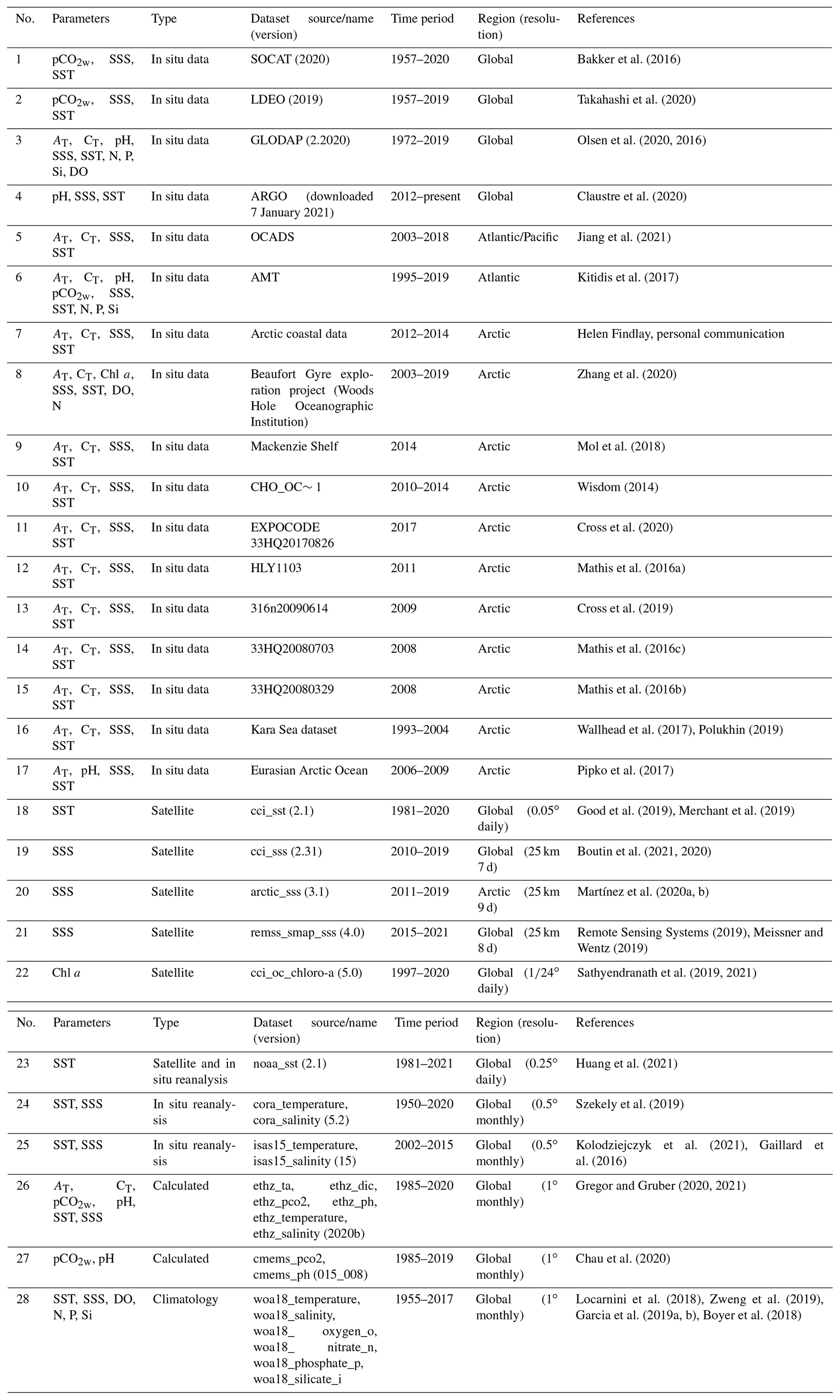
Figure 1Numbers of carbonate system measurements included in the database per year. (a) Seawater pCO2, (b) total alkalinity (AT), (c) dissolved inorganic carbon (CT) and (d) pH.
Sequential processing of all in situ data is a major task that would take several weeks to complete on a normal personal computer, a situation that is likely to worsen as data volume continues to increase. To speed up processing, we initiated ROI definition from different times. A start year and month is specified, and ROIs are defined using only in situ data starting from that time. In this way, the task can be divided into parallel processing streams. Initial ROI definitions in each stream are in general different from those that would be generated sequentially from the start, so care must be taken in combining ROIs generated from different start times. The approach we have adopted is to allow processing from an earlier start time to continue past the start time of the next processing stream, creating two concurrent ROI sets covering the same time period. The concurrent period is inspected for sequences of ROIs that are identical in the two sets of results. If such a sequence is more than 10 d long, ROIs from the earlier stream before the identical sequence cannot overlap with those from the later stream after the identical sequence, and so it is safe to merge the streams. If an identical sequence more than 10 d long cannot be found, ROIs from the earlier stream before the longest identical sequence can be compared individually with those from the later stream after the identical sequence to ensure that none overlap. The merged data are stored in yearly netCDF files.
3.3 Creating the OceanSODA-MDB matchup database
Felyx is a tool created to extract data from along-track, swath or gridded datasets such as Earth observation (EO) data over defined ROIs (https://felyx.gitlab-pages.ifremer.fr/felyx_docs/, last access: 20 February 2023). Felyx is a free software solution, written in Python, the aim of which is to provide Earth observation data producers and users with an open-source, flexible and reusable tool to allow scientific analysis and performance monitoring of scientific data through subsetting over specific areas or matching up with in situ measurements. The development of felyx is supported by Copernicus, the European Union's Earth observation programme.
Felyx is used in this context to extract EO, model, climatology and reanalysis data within maximum-sized ROIs centred on the in situ ROIs. Given the time and location of a ROI, felyx is able, for each EO data source, to extract observation subsets within a 50 km radius and ±5 d from the ROI's centre time and location (Fig. 18).
Hence matchup data are all extracted over the same size regions centred on matching in situ data. This methodology ensures that all data being compared (e.g. satellite and in situ observations) are treated as consistently and equally as possible, allowing all uncertainties in all observations to be included within the analysis. The resultant radial matchup data (the output from the felyx system) are stored in the same NetCDF files used for the in situ data. For each averaged parameter, the mean, median, standard deviation, minimum, maximum, interquartile range and sample count of the observations found within the ROI's search area and time frame are calculated and provided. Finally, the output files are enriched with metadata for traceability in compliance with the Climate and Forecast Convention and self-description of the content, and the units are harmonised across the different in situ and Earth observation sources.

Figure 2Numbers of ROIs per year (bars) included in the database containing measurements of each carbonate system parameter and the mean number of measurements per ROI (lines), for (a) pCO2w, (b) total alkalinity (AT), (c) dissolved inorganic carbon (CT) and (d) pH.
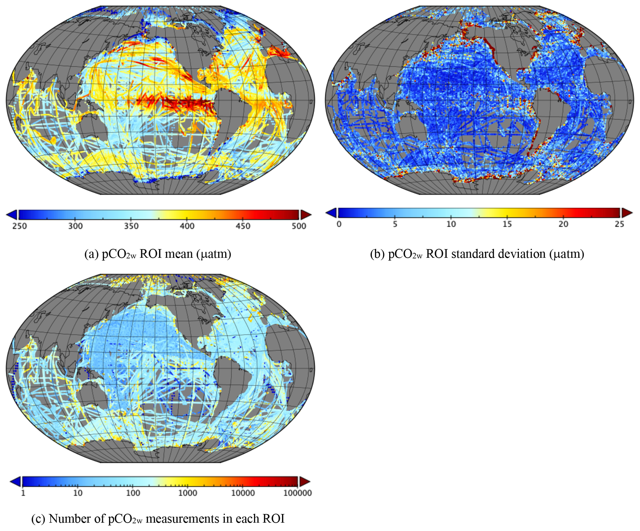
Figure 3Statistics of pCO2w in each ROI over the whole database (272 753 ROIs). (a) ROI mean, (b) ROI standard deviation and (c) number of measurements in each ROI.

Figure 4Statistics of AT in each ROI over the whole database (13 595 ROIs). (a) ROI mean, (b) ROI standard deviation and (c) number of measurements in each ROI.
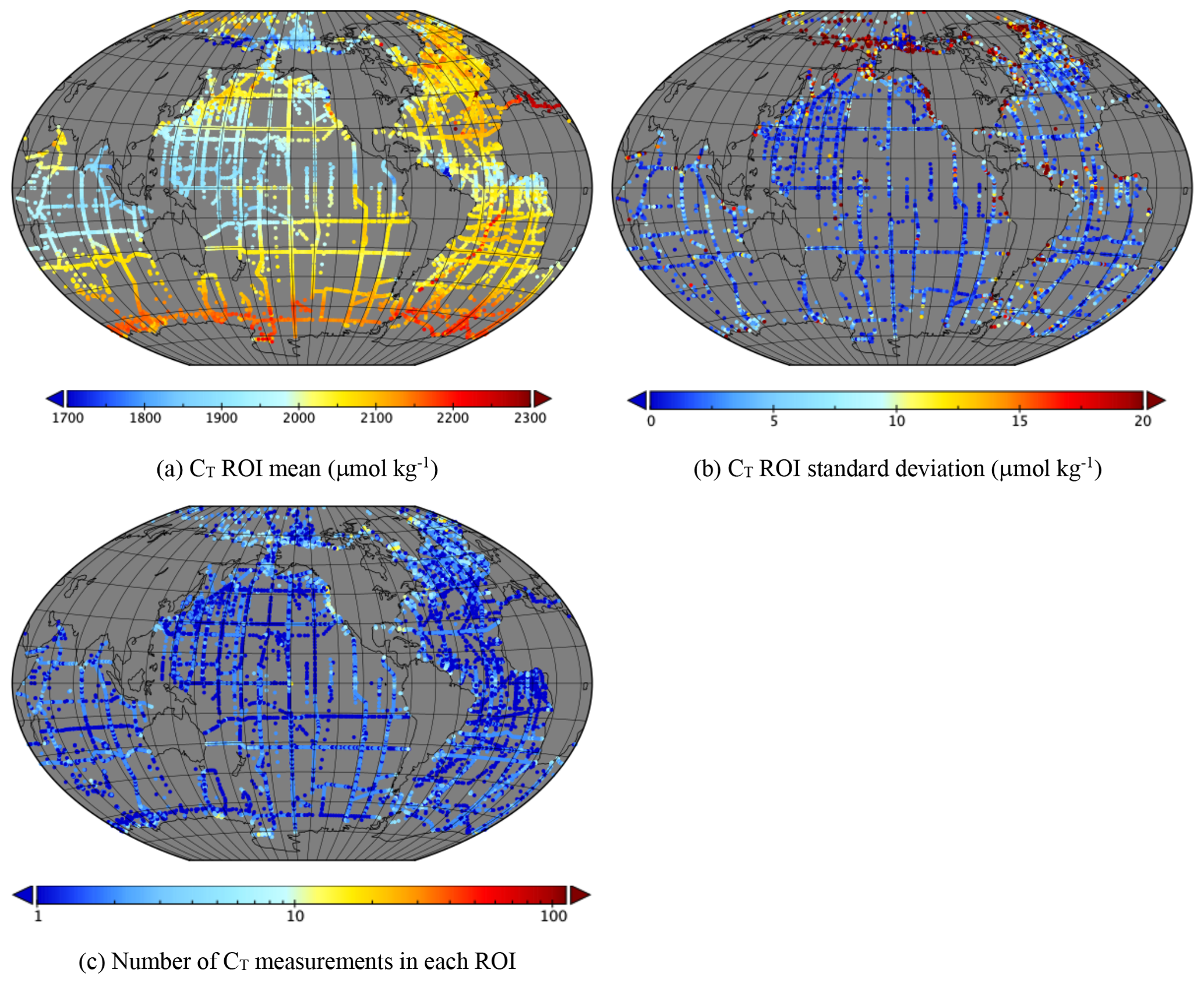
Figure 5Statistics of CT in each ROI over the whole database (15 041 ROIs). (a) ROI mean, (b) ROI standard deviation and (c) number of measurements in each ROI.
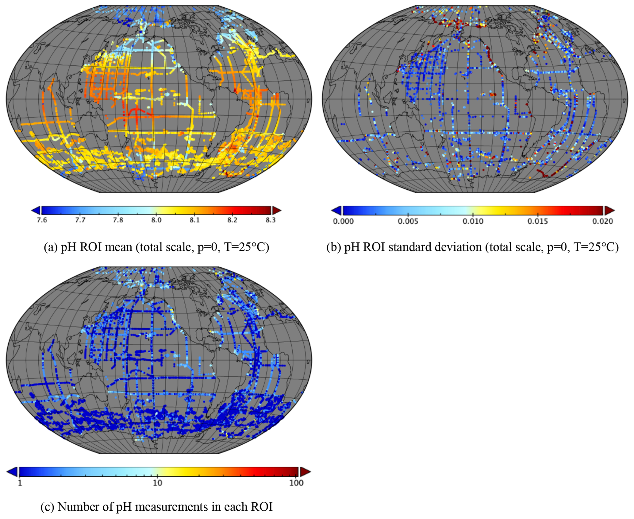
Figure 6Statistics of pH in each ROI over the whole database (19 613 ROIs). (a) ROI mean, (b) ROI standard deviation and (c) number of measurements in each ROI.
The collated input dataset contains 34 912 843 individual stations, of which 34 839 413 (99.8 %) contain pCO2w, 24 474 (0.07 %) contain AT, 27,032 (0.08 %) contain CT and 21 924 (0.06 %) contain pH (note that stations may contain more than one carbonate system parameter). Based on the ROI definition of 100 km radius and 10 d duration, this collated dataset resulted in 285 822 ROIs, of which 272 753 (95.4 %) contain pCO2w, 13 595 (4.8 %) contain AT, 15 041 (5.3 %) contain CT and 19 613 (6.9 %) contain pH. Dates range from 1957 (pCO2w) to December 2020 (pH) (missing years from 1959 to 1971 contain no in situ data), with steep increases in the number of measurements in the 1990s and further increases in pCO2w measurements in the early 2000s and in pH measurements in the 2010s, the latter associated with the recent development of autonomous pH sensors such as in the Bio-ARGO programme (Fig. 1; note the logarithmic scale). The recent reduction in AT and CT measurements may be associated with the situation that, unlike pCO2w and pH, all AT and CT measurements in the dataset are performed in the laboratory, resulting in a delay in data submission. There may also be a reduction in support for core laboratory measurements as new autonomous measurements become available, although some will still be necessary for validating and calibrating autonomous sensors.
The total number of measurements is not necessarily a good indication of representativity, especially with the advent of flow-through pCO2w instruments which can collect many measurements spanning a small spatiotemporal range. In this respect, the number of ROIs is a better guide. Fig. 2 (note the linear scale) shows the number of ROIs per year and the mean number of measurements per ROI, which is typically around 2 except in the case of pCO2w, for which it increases from around 10 in the 1980s to over 200 in 2019. Since the advent of Bio-ARGO, which typically delivers one surface pH measurement per ROI, while cruises typically deliver more than one, the proportion of ROIs with one pH measurement has increased, and the mean number of pH measurements per ROI has decreased, and this is likely to continue as the number of Bio-ARGO floats increases.
Figures 3 to 6 show the mean, standard deviation (where a ROI contains more than one measurement) and number of measurements in each ROI over the whole dataset. Note that the standard deviation is only over a 10 d period and so does not show variability on longer timescales, such as seasonality or interannual variability. Note also that these plots include ∼270 000 points in the case of pCO2w, and more recent measurements overlay older ones, so specific features seen in these plots should be checked in more detail. Variability is greatest in coastal regions and in parts of the Arctic, for example, the Beaufort, East Siberian and Laptev seas and between Greenland and Svalbard.
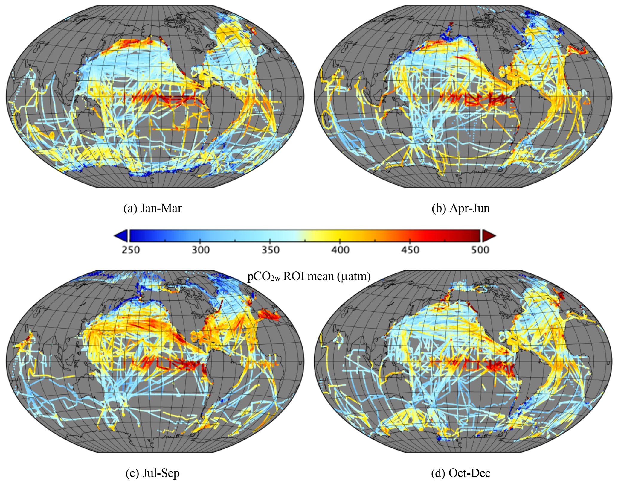
Figure 7Mean pCO2w (µatm) divided into seasons. (a) January–March (70 658 ROIs), (b) April–June (67 631 ROIs), (c) July–September (69 083 ROIs) and (d) October–December (65 381 ROIs).
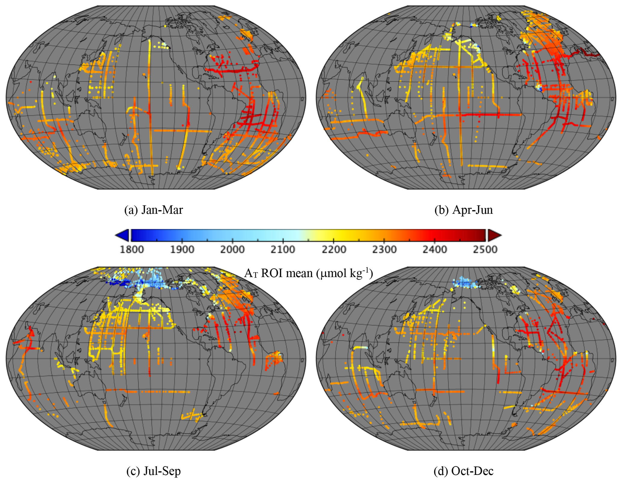
Figure 8Mean AT (µmol kg−1) divided into seasons. (a) January–March (3602 ROIs), (b) April–June (3682 ROIs), (c) July–September (3960 ROIs) and (d) October–December (2351 ROIs).
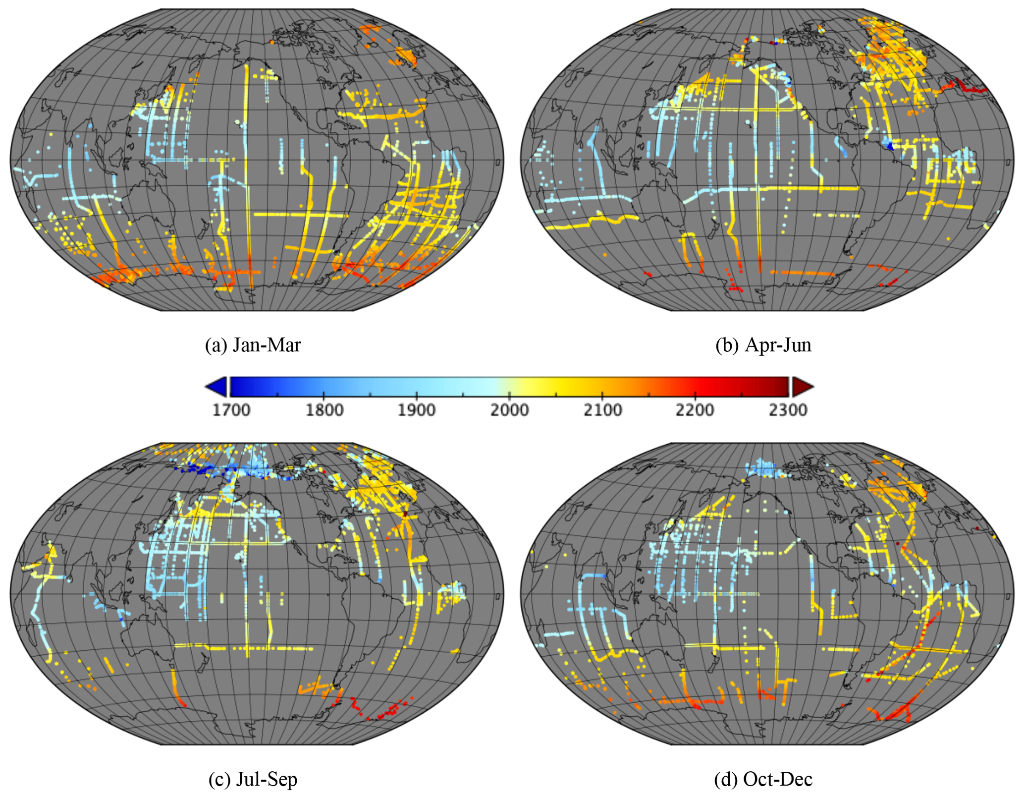
Figure 9Mean CT (µmol kg−1) divided into seasons. (a) January–March (4029 ROIs), (b) April–June (4256 ROIs), (c) July–September (4197 ROIs) and (d) October–December (2559 ROIs).
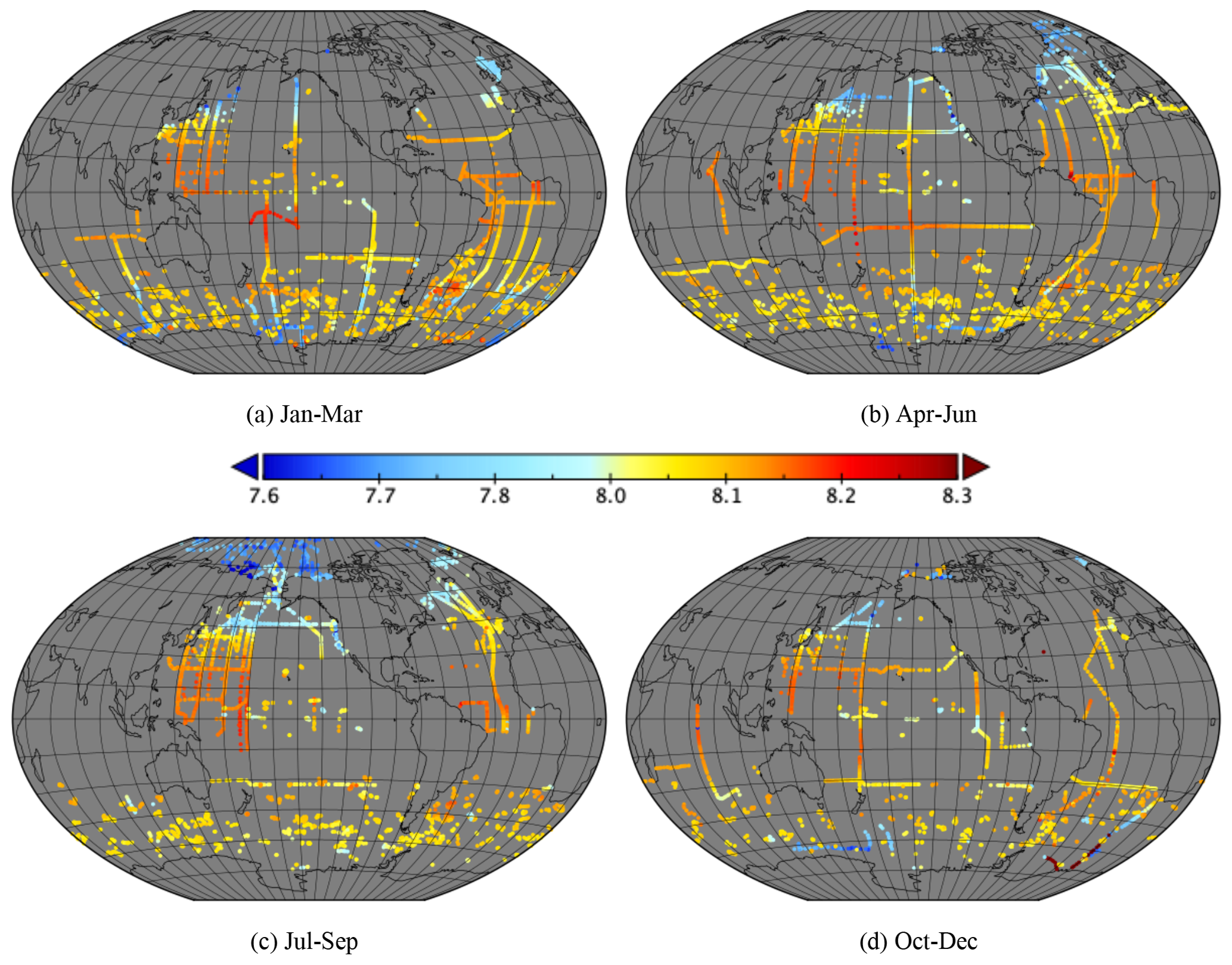
Figure 10Mean pH (total scale, p=0, 25 ∘C) divided into seasons. (a) January–March (5501 ROIs), (b) April–June (5386 ROIs), (c) July–September (4959 ROIs) and (d) October–December (3767 ROIs).

Figure 11Mean pCO2w (µatm) divided into decades: 1751 ROIs to 1969, 1636 in the 1970s, 9090 in the 1980s, 42 548 in the 1990s, 97 313 in the 200s and 120 415 from 2010 to 2020.
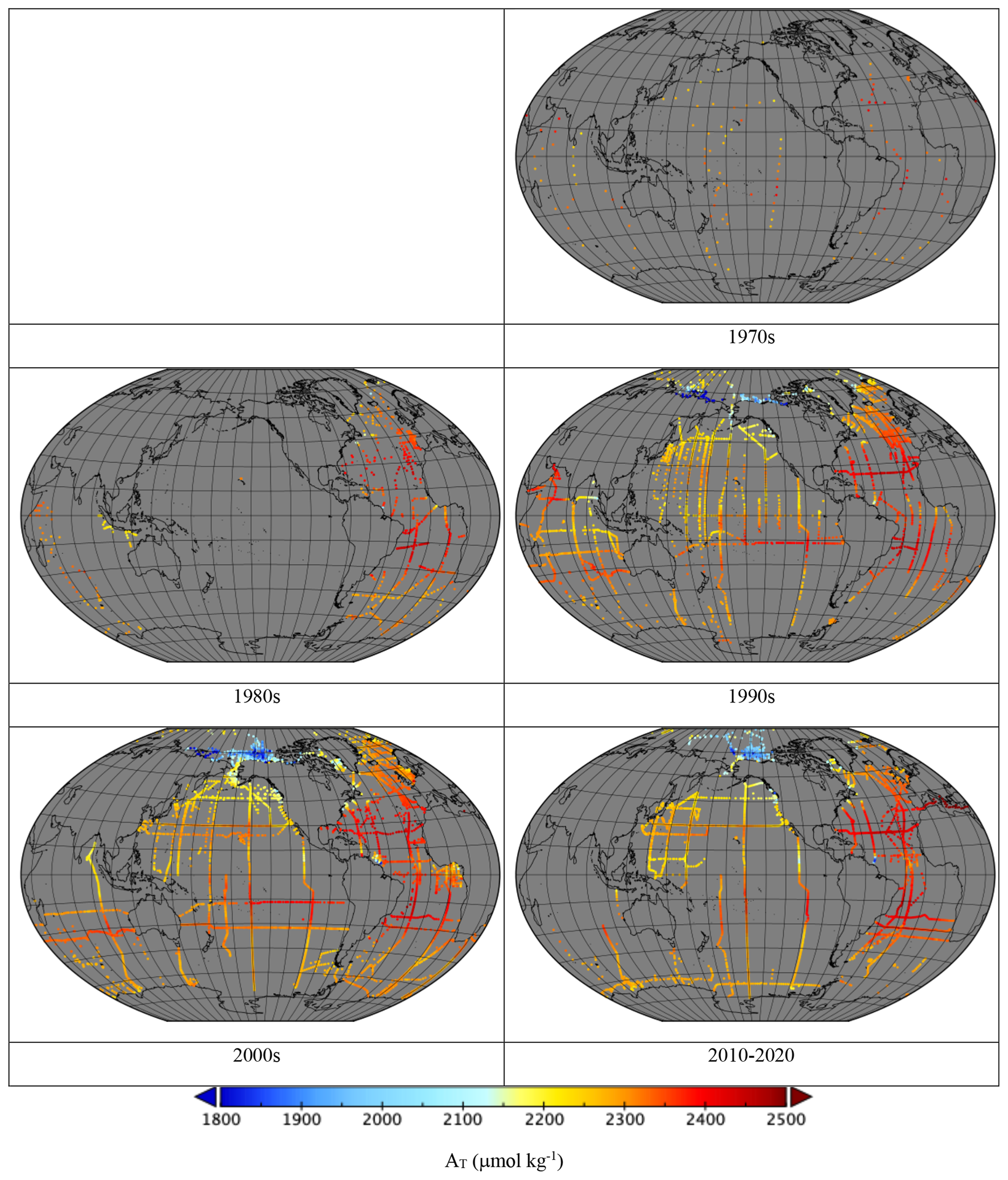
Figure 12Mean AT (µmol kg−1) divided into decades: 128 ROIs in the 1970s, 707 in the 1980s, 3923 in the 1990s, 5196 in the 2000s and 3641 from 2010 to 2020.
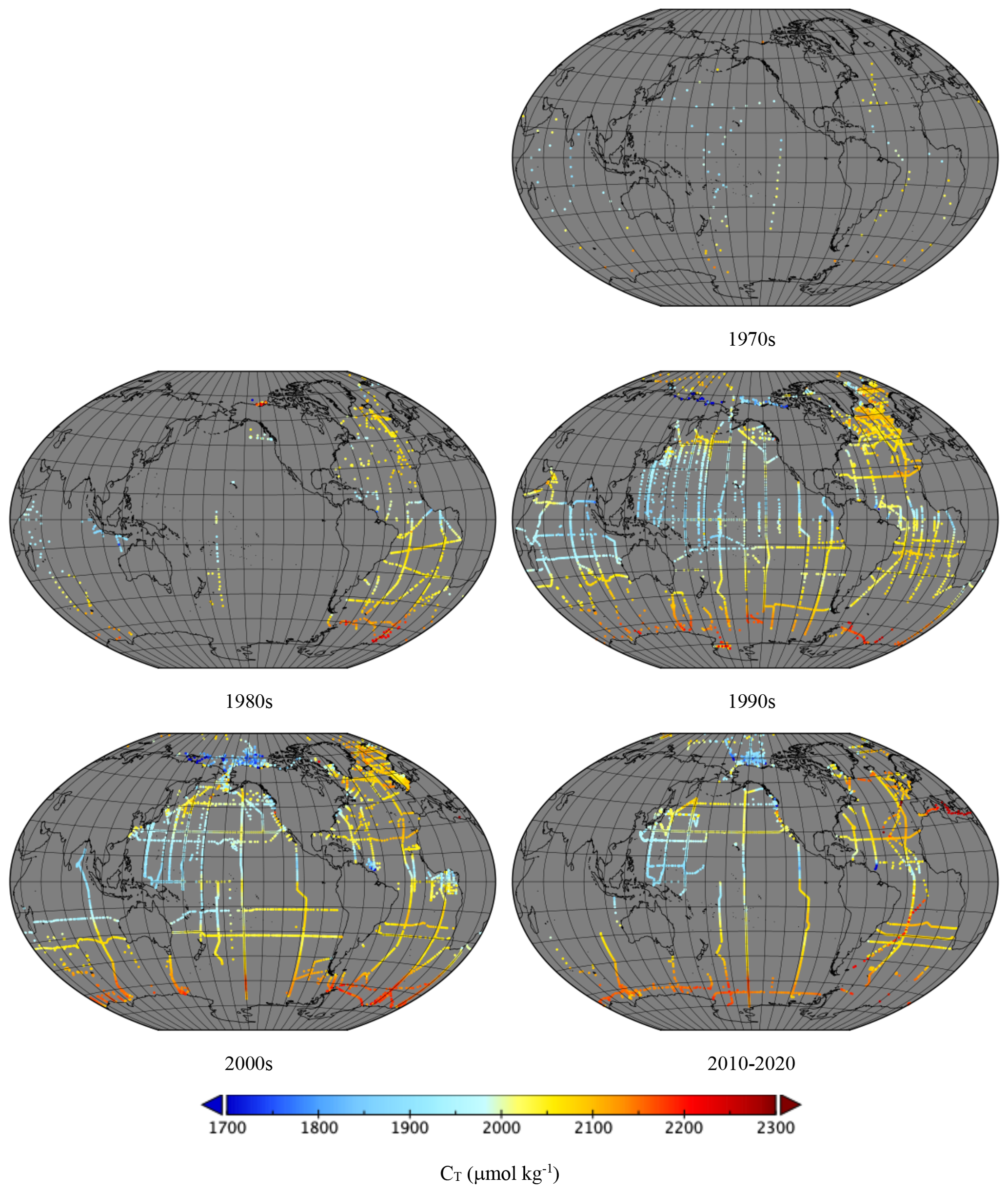
Figure 13Mean CT (µmol kg−1) divided into decades: 123 ROIs in the 1970s, 971 in the 1980s, 4613 in the 1990s, 5672 in the 2000s and 3662 from 2010 to 2020.
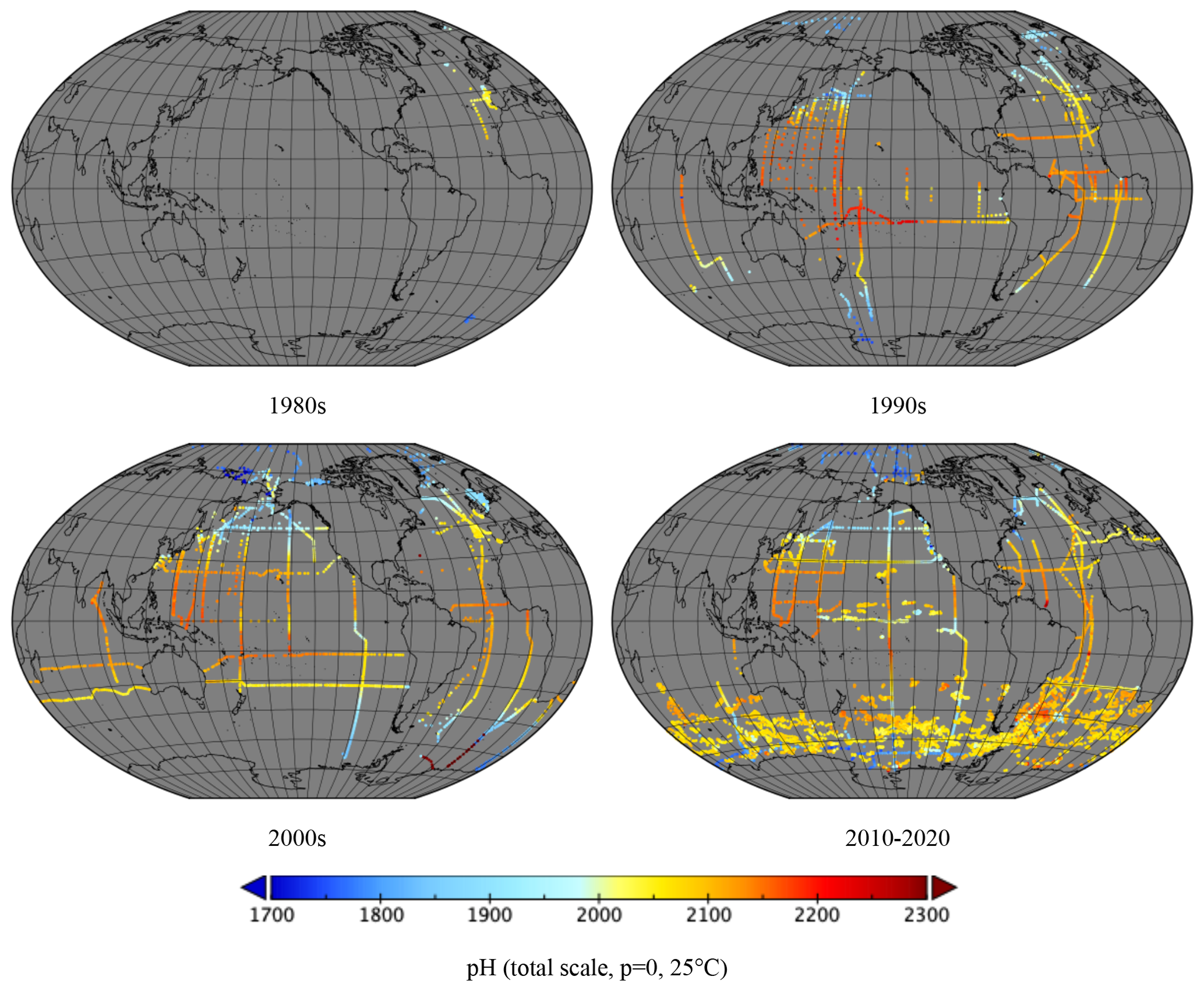
Figure 14Mean pH (total scale, p=0, 25 ∘C) divided into decades: 120 ROIs in the 1970s, 672 in the 1980s, 3428 in the 1990s, 4632 in the 2000s and 10 761 from 2010 to 2020.
Figures 7 to 10 show the mean in each ROI divided into seasons. Strong pCO2w seasonality is evident in the Northern Hemisphere, with high values in the northern Pacific and Atlantic in January–March and in the subtropics in July–September. Seasonality is less clear in CT and pH, which may be due to the lower data density. This may also be due to the relatively smaller amplitude of seasonal changes with respect to the mean; for example, in Kitidis et al. (2017) a 6 % increase in pCO2w results in a 0.7 % increase in CT and 0.3 % decrease in pH over 19 years. We would only expect strong seasonality in AT where there are large seasonal variations in salinity or strong terrestrial influence.
Figures 11 to 14 show the mean in each ROI divided into decades. As well as the increases in data density, the increase in pCO2w with time is clearly visible. The recent Bio-ARGO measurements can clearly be seen as a “speckle” pattern in the Southern Ocean in 2010–2020 pH.
To illustrate the use of the MDB, we present a reparameterisation of the Takahashi et al. (2014) (T14) global algorithm for potential alkalinity (PA), which is equal to AT plus nitrate. A parameterisation of pCO2w, which has much higher data density, would better illustrate the advantages of the MDB approach, but we could find no simple, global pCO2w algorithm that could be reparameterised as T14 can. For this we use in situ AT and SSS and WOA monthly climatological nitrate, since this is what would be needed to produce synoptic maps of AT, for example, from satellite or model SSS. The T14 algorithm is clearly not intended for application to extreme coastal waters, of which there are many in the MDB, and algorithm uncertainties are expected to increase if we include waters with coastal or benthic influence, but T14 offer no criteria to distinguish these. Sasse et al. (2013) presented their own algorithms for AT and CT, and they used the criteria that waters should be considered free from coastal influence (“marine”) if greater than 300 km from the nearest shore with water depth greater than 500 m. These thresholds are global and likely to be over-conservative in many regions. Here we adapt these criteria, aiming for a marine definition that is as inclusive as possible while not significantly compromising the fit found in highly marine waters and providing a separate fit for the remaining coastal waters.
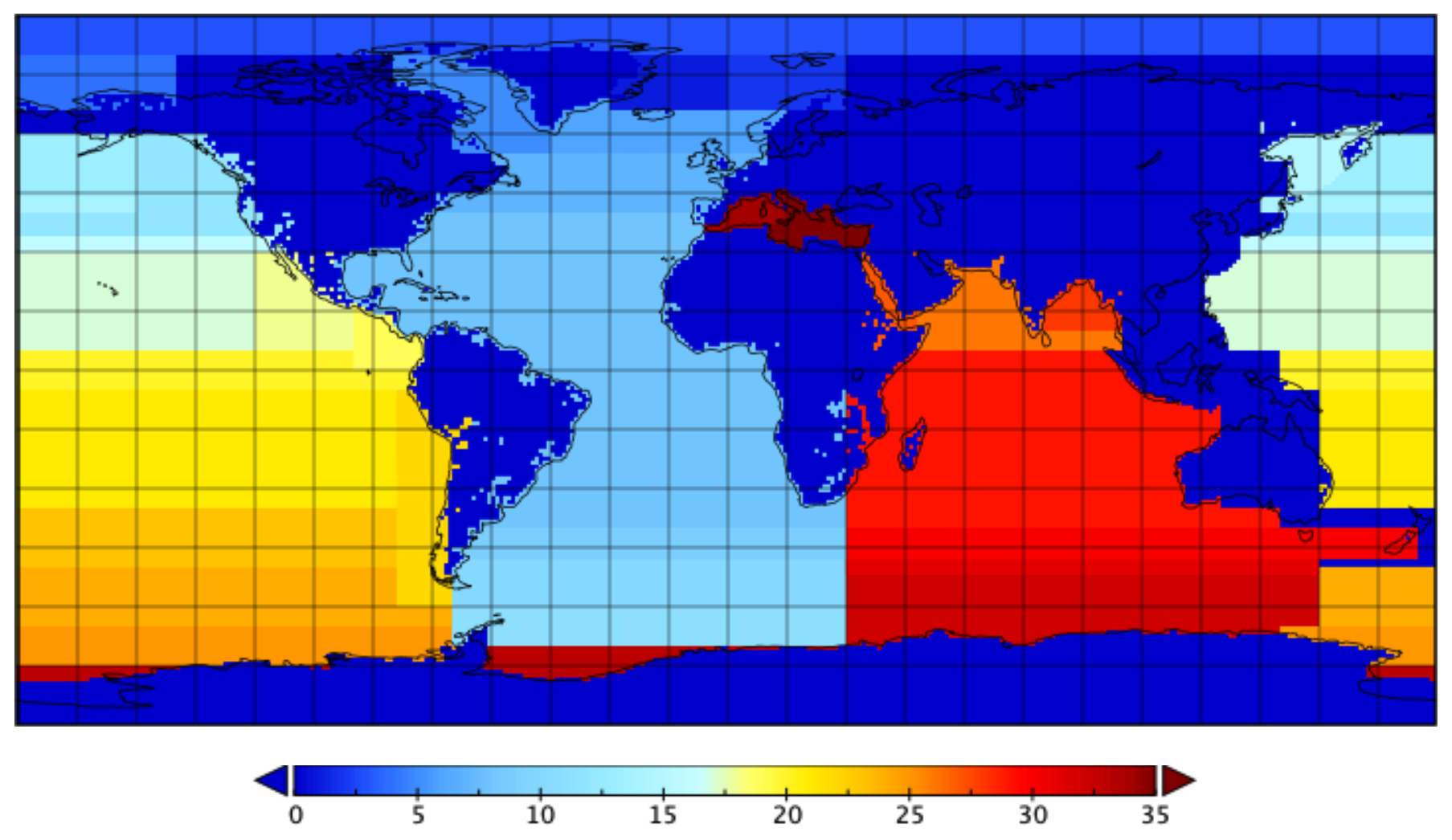
Figure 15Regions used in reparameterisation of Takahashi et al. (2014). See Table 2 for region names.
The T14 regions we use are shown in Fig. 15 and mapped on a 1∘ grid in supplementary data. We have eliminated overlaps in the original T14 regions, adjusted some boundaries to align more closely with geographical boundaries, and added the western and eastern basins of the Mediterranean Sea. We now subdivide the data in order to distinguish marine from coastal and to perform cross-validation. It should be noted that this subdivision is done as a “user” of the MDB. The subdivision used to create the MDB minimises the effect of differences in data density, while the subdivision described below is at a coarser scale and done for different reasons. In each T14 region, we divided the data into marine and coastal domains, initially defining marine as having distance from the nearest shore greater than D=300 km and water depth greater than Z=500 m. The data in each domain were divided into up to 10 subsets for cross-validation using the following methodology. If the number of marine data in a region is less than 10, the (up to) 10 points with greatest min(distance from coast D, water depth Z) are defined as marine, and D and Z decreased by the minimum required to ensure that the new marine data meet the marine definition. The data are divided into years, with the time series from HOT and BATS being labelled as “year” 0 and 1, respectively. If this results in more than 10 subsets, the subsets with lowest occupancy are combined, with the proviso that adjacent years cannot share the same subset. This prevents early years, HOT and BATS, which tend to have lower data density, from all being combined into a single subset and prevents HOT and BATS from being merged. This continues until the number of subsets is reduced to 10. If the number of yearly subsets is less than 10, each data point is given its own subset unless this results in more than 10 subsets, in which case data are assigned randomly to 10 subsets with as equal data numbers as possible. If the final number of subsets is less than five, fitting is not attempted. If fitting occurs in one domain but not the other, the fit parameters are applied to the other domain (shown as brackets in Table 2).
Table 2Quoted and calculated RMSE values in each region defined by Takahashi et al. (2014) (T14) partitioned into coastal and marine subregions (see Table 3 for definitions). Calculated values are for the original T14 coefficients (RMSE T14), the coefficients recalculated using the MDB with cross-validation (RMSE new) and the RMS difference between the two over the MDB data (RMSdif).

Error analysis is done using cross-validation, training the T14 relationship PA = A SSS + B on all but one of the subsets using singular-value decomposition linear regression, then the error (difference between the resulting fit and the data) at each point of the remaining validation subset is recorded. This process is repeated using a different validation subset each time, giving an error for every data point. These errors are used to calculate the following summary statistics: root mean squared error (RMSE), mean absolute error (MAE), median absolute error (MDE), and mean and median error (both measures of bias).
To check whether the marine definition was over-conservative, we first defined an acceptable level of degradation in marine RMSE (RMSEm) in exchange for an expansion of the marine domain, RMSEmax= max(RMSEm+0.1, RMSEm⋅1.01). We then repeated the following procedure iteratively. We sorted the coastal data by either distance from coast or water depth, then converted the points with maximum distance or depth to marine if their absolute error was not greater than RMSEm, meaning that the addition of the points would not increase RMSEm. D and Z were adjusted if necessary to ensure that the new marine data obeyed the marine criteria, and marine and coastal fits and statistics were recalculated. If the resulting marine RMSE was less than the lowest RMSEm found so far, RMSEmax was recalculated. Next, we tried going beyond the coastal data with absolute error greater than RMSEm, continuing to lower distance or depth until the absolute error again exceeded RMSEm but with opposite sign. Adjusted fits were calculated separately for adjustments of distance and depth, and for both combined, and the new fit with lowest marine RMSE was accepted if the marine RMSE was no more than RMSEmax, again adjusting D and Z and recalculating RMSEmax if necessary. This procedure was repeated until it resulted in no change from coastal to marine.
Table 3Slope and intercept in each region defined by Takahashi et al. (2014) (T14). Original coefficients quoted by T14 are labelled T14, and reparameterised coefficients are given for coastal and marine subregions, where a point is marine if both distance from coast and water depth are greater than their regional thresholds.
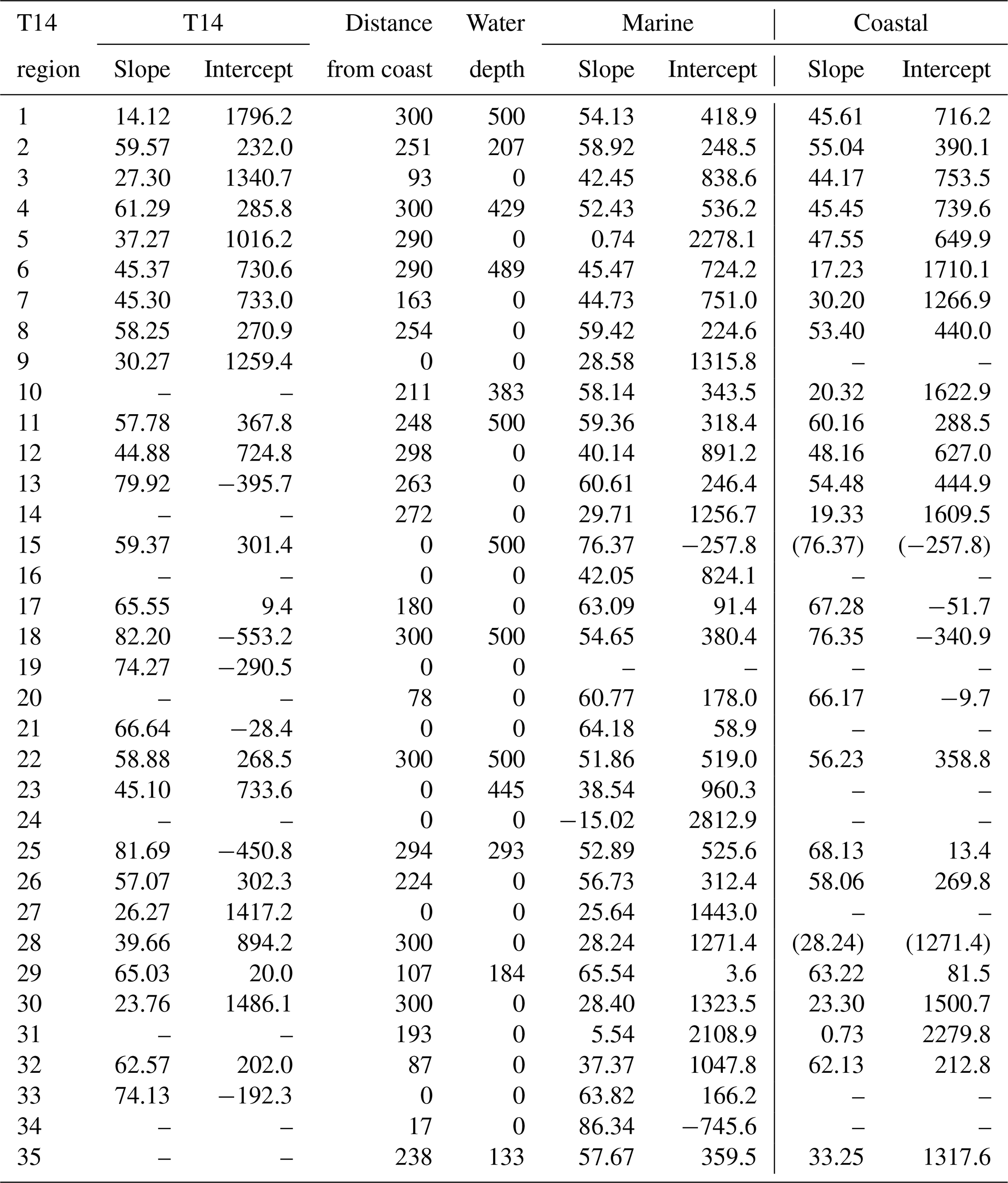
Results are shown in Tables 2 and 3. Table 2 shows the region names, the RMSE of the original T14 and reparameterised algorithms in the marine and coastal domains, and the root mean squared difference (RMSdif) between the T14 and new algorithms, a measure of the extent to which results have changed due to the reparameterisation. Note that the RMSE of the original algorithm includes data used by T14 in the original fit and so may be an underestimate, while that of the new algorithm is calculated using cross-validation. This can result in the new RMSE being greater than the T14 RMSE despite the refitting. Table 3 gives details of the algorithms, including the thresholds of distance from coast and water depth used to define the marine domain and the slope and intercept in each region and domain. Globally, the marine RMSE was reduced from 15 µmol kg−1 (likely to be an underestimate; see above) using the original T14 algorithm to 12 µmol kg−1, while in coastal waters the RMSE was reduced from 32 to 23 µmol kg−1 using only data for which T14 makes a prediction but reduced further to 22 µmol kg−1 when using all data.
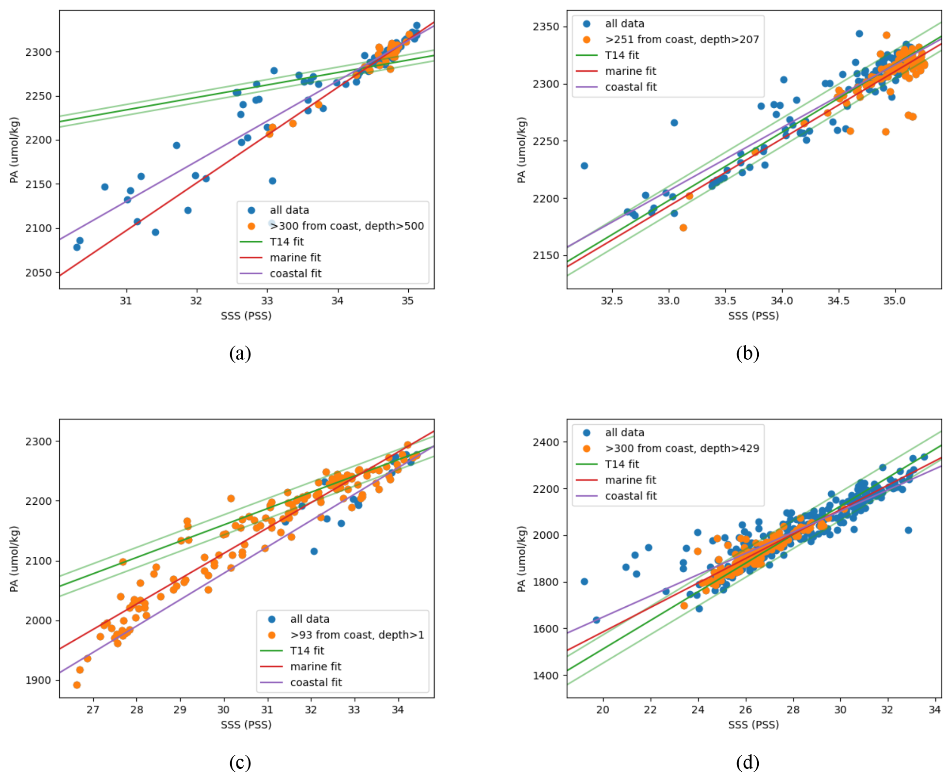
Figure 16PA–SSS relationships in the first four T14 regions, all in the Arctic. Orange data are classified as marine, based on the distance from the nearest coast in kilometres and the depth in metres both being greater than region-specific thresholds. All other data (in blue) are classified as coastal. The thick green line is the T14 relationship, and the thin green lines show the T14 quoted RMSE. The red and purple lines are the new fits to marine and coastal data. (a) Region 1, West GIN Seas; (b) region 2, East GIN Seas; (c) region 3, High Arctic; (d) region 4, Beaufort Sea.
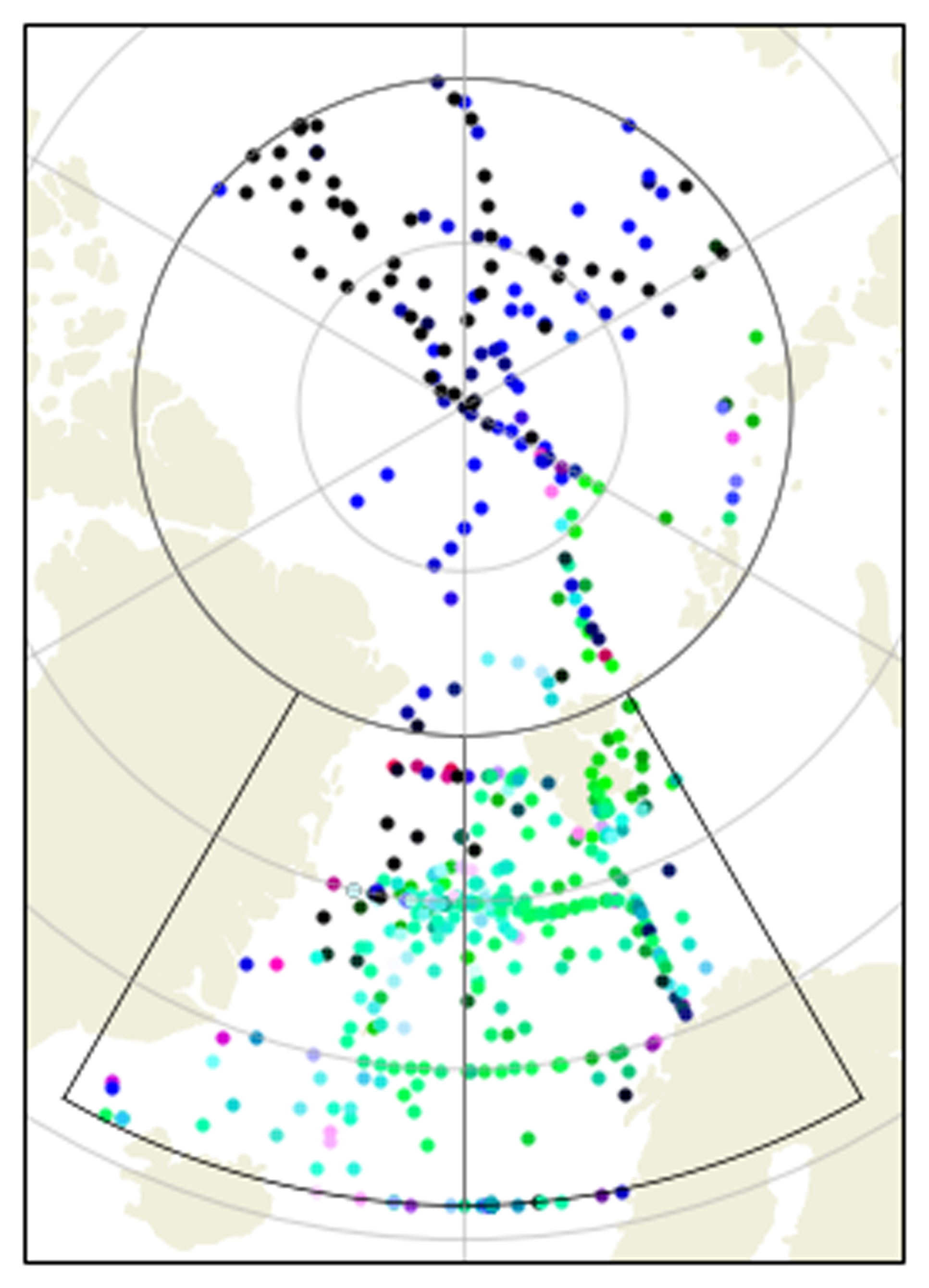
Figure 17T14 regions 1 (West GIN Seas, bottom left), 2 (East GIN Seas, bottom right) and 3 (High Arctic, top) with corresponding MDB data. Each point is coloured according to the probability density of a Gaussian with mean equal to the T14 regression and standard deviation equal to its quoted RMSE, which is a measure of how consistent the data are with the T14 fit. The red component is the consistency with the region 1 fit, green with the region 2 fit and blue with the region 3 fit.
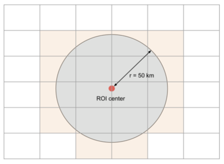
Figure 18Spatial colocation principle for Earth observation data. All gridded observations within or intersecting a 50 km radius from the ROI centre for all the consecutive files within ±5 d around the ROI centre time are averaged together. The mean and other statistics (median, standard deviation, minimum, maximum and interquartile range) are also calculated and provided in the output matchup dataset.
The greatest marine RMSdif (49 µmol kg−1) occurred in T14 region 3 (High Arctic) and the next greatest (20 and 18 µmol kg−1) in regions 1 and 4 (West GIN Seas and Beaufort Sea), all other regions having marine RMSdif less than 11 µmol kg−1. Note that in some cases the coastal RMSdif is less than the marine RMSdif, suggesting that the T14 fit was dominated in these regions by data that we classify as coastal. The fits in regions 1 to 4 are shown in Fig. 16. In region 1 the tightly linear data used by T14 are not present in the MDB, and the few data that are consistent with the T14 relationship are all coastal, while the rest of the data (marine and coastal) follow similar relationships to those in region 2 (T14 Fig. 3, West and East GIN Seas). The data in region 3 are mostly marine, and while the data used by T14 mostly follow a relationship also seen in some of the MDB data, most of the MDB data follow another relationship, barely seen in the T14 data and consistent with the relationships seen in region 2 (T14 Fig. 3, High Arctic and East GIN Seas). In region 4, the T14 and reparameterised relationships are quite consistent with each other, the large RMSdif being mainly due to the large variability in this region. T14 also note that some of their region 1 data follow the region 2 relationship, which they ascribe to eddies from region 2. One explanation might be that these eddies have become more frequent since the data used by T14, another that the water mass corresponding to region 2 (Atlantic waters flowing north into the Arctic) has expanded west into region 1 and north into region 3. To test this, Fig. 17 shows a map of regions 1, 2 and 3 with data points coloured red, green and blue in proportion to the probability density of a Gaussian distribution with mean and standard deviation equal to the T14 prediction and its RMSE in T14 regions 1, 2 and 3, respectively. Hence a red point would be consistent with the T14 region 1 prediction and inconsistent with that of regions 2 and 3, a white point would be consistent with all three predictions, and a black point would be inconsistent with all three. This map indicates that only a narrow strip close to the Greenland coast follows the T14 region 1 relationship, the rest being more consistent with region 2, that the region 2 relationship remains more plausible than the region 3 relationship up to about 86∘ N and that the region 3 relationship performs poorly in the Beaufort Sea sector between 130 and 180∘ W.
This exercise has shown success in improving the fit of T14, incorporating new data, clarifying the distinction between marine and coastal domains and providing an optimal fit in marine areas and a generally poorer fit in coastal areas, with estimated uncertainties.
In order to stay relevant, the MDB must be regularly updated. Updates to the MDB can be made by adding new data to the existing ROIs, only creating new ROIs where necessary. This enables the MDB to be updated much more quickly and easily that recalculating all ROIs from the beginning. As well as inclusion of new data, this process allows updating of data already in the MDB, for example, if an existing dataset is reprocessed. The scale of the ROIs (100 km diameter, 10 d duration) was chosen based upon our knowledge of the datasets used, the likely spatial and temporal scales of changes in these data and conditions, and the desire to ensure we have matchups between the in situ ROIs and the other datasets. These scales are adjustable, and regional MDBs may be created on smaller spatiotemporal scales in regions where this scale is inappropriate. This MDB is focused on the surface carbonate system, and only ROIs containing carbonate system variables are included, but the same methodology can be used to create MDBs for other parameters of interest, such as methane or dimethyl sulfide or an MDB based purely on a single parameter like salinity, or SST.
It should be borne in mind that oceanic processes can have strong effects on smaller scales than the MDB; for instance, a growing phytoplankton bloom might significantly change surface pCO2w over a 10 d period. These effects are potentially detectable in the MDB through, for example, the standard deviation of pCO2w but in general will be masked by the averaging inherent in the MDB method (the same is true for any gridding or averaging approach). Other effects such as surface temperature gradients affecting pCO2w (Woolf et al., 2016) will be similarly masked by averaging over the top 10 m within the current MDB. The MDB approach might be inappropriate if the subject of study is highly dependent on sub-ROI effects, such as a study of the depth variation of pCO2w in the surface layer, and in such cases it would be better to use individual measurements. It should also be borne in mind that averaging will not remove biases (e.g. regional or seasonal) from the in situ data, though it will reduce stochastic noise.
The reparameterisation described in Sect. 5, though successful, could have been done with the original AT measurements from the original sources, probably with similar results because the data density of AT measurements is typically low. Over 50 % of MDB regions with AT contain only one AT measurement, and only 1 % contain 10 or more. The real distinction between the MDB approach and use of individual data points comes when comparing data with very high and low densities, which are more likely to be found in parameters that can be measured at high frequency, such as pCO2w. To illustrate, consider the hypothetical example of a little-studied sea to which we wish to apply a simple model of constant pCO2w. We have data from two cruises, one in winter making a transect of 10 discrete samples and the other in summer with an underway system making a transect of 1000 samples. The actual pCO2w has a mean of 400 µatm but with a seasonal cycle from 375 to 425 µatm not accounted for by our simple model. If the 10 winter measurements average to 375 µatm and the 1000 summer measurements to 425 µatm, simple averaging of all data gives an estimate of just under 425 µatm, while if the 1000 samples are binned into 10 regions of 100 measurements each, the correct average is found. Although this example is unrealistic, it is representative of the problems that can occur when fitting models to unevenly distributed data. The models are more complex and the deviations less obvious, but if there are systematic effects not captured by the model, and the data density is greater towards one side of the distribution of these effects, then the model becomes biased. The best way to overcome this is to identify the biasing effects and account for them (e.g. a seasonal split in the example), but some will always remain. The MDB approach lessens the effect of unaccounted biases by evening out differences in data density as consistently as possible.
All data are freely available on the IFREMER data repository at https://doi.org/10.12770/0dc16d62-05f6-4bbe-9dc4-6d47825a5931 (Land and Piollé, 2022).
Code will be made available by the authors on reasonable request.
Here we present a global dataset created using a novel methodology for combining different dataset types (e.g. in situ, model, satellite) onto the same spatial and temporal scales using “regions of interest” (ROIs). This method gives advantages over previous methods, which predominantly grid data by latitude and longitude, as it provides a uniform spatiotemporal resolution across the globe and minimises biases created by differences in data density. We have collated a large global dataset comprised primarily of publicly available in situ, satellite and climatological data; processed it using this methodology; and presented summary statistics describing the results. The resulting matchup database (OceanSODA-MDB) is suitable for reparameterising empirical algorithms, as demonstrated here, but would also enable validation, evaluation and performance assessment of satellite data, reanalysis or model datasets, as well as model–data intercomparisons, by simply adding these data into the existing MDB.
PEL and JDS developed the initial database concept, and then PEL created all methods for the in situ dataset collation and region definitions and then wrote the initial manuscript. HSF collated all in situ datasets and identified the quality control procedures and uncertainty values. JFP developed all felyx aspects and collated all satellite, model and reanalysis data. HG and RS tested the resulting database. VK contributed AMT data. AP collected the Kara Sea dataset, screened the data and assessed the possibility of using Russian data due to differences in methods for determining pH and total alkalinity. IIP collected Arctic data. All authors contributed to the manuscript.
The contact author has declared that none of the authors has any competing interests.
Publisher's note: Copernicus Publications remains neutral with regard to jurisdictional claims in published maps and institutional affiliations.
The Surface Ocean CO2 Atlas (SOCAT) is an international effort, endorsed by the International Ocean Carbon Coordination Project (IOCCP), the Surface Ocean Lower Atmosphere Study (SOLAS) and the Integrated Marine Biosphere Research (IMBeR) programme, to deliver a uniformly quality-controlled surface ocean CO2 database. The many researchers and funding agencies responsible for the collection of data and quality control are thanked for their contributions to SOCAT. We are also greatly indebted to all who contributed their efforts to the GLODAP project. Bio-ARGO data were collected and made freely available by the international Argo project and the national programmes that contribute to it. We thank the UK National Environment Research Council for funding the Atlantic Meridional Transect (Climate Linked Atlantic Sector Science, CLASS).
This research has been supported by the European Space Agency (grant no. 4000112091/14/I-LG), a Grant of the President of the Russian Federation for state support of young Russian scientists (grant no. MK-3506.2022.1.5) and the Russian Science Foundation (grant no. 21-17-00027). Publisher's note: Copernicus Publications has not received any payments from Russian or Belarusian institutions for this paper.
This paper was edited by Giuseppe M. R. Manzella and reviewed by three anonymous referees.
AMAP: AMAP Assessment 2018: Arctic Ocean Acidification, viii + 99 pp-viii + 99 pp., https://doi.org/10.1016/j.techfore.2013.08.036, 2018.
Argo: Argo float data and metadata from Global Data Assembly Centre (Argo GDAC), SEANOE, https://doi.org/10.17882/42182, [data set], last access: 7 January 2021.
Bakker, D. C. E., Pfeil, B., Landa, C. S., Metzl, N., O'Brien, K. M., Olsen, A., Smith, K., Cosca, C., Harasawa, S., Jones, S. D., Nakaoka, S., Nojiri, Y., Schuster, U., Steinhoff, T., Sweeney, C., Takahashi, T., Tilbrook, B., Wada, C., Wanninkhof, R., Alin, S. R., Balestrini, C. F., Barbero, L., Bates, N. R., Bianchi, A. A., Bonou, F., Boutin, J., Bozec, Y., Burger, E. F., Cai, W.-J., Castle, R. D., Chen, L., Chierici, M., Currie, K., Evans, W., Featherstone, C., Feely, R. A., Fransson, A., Goyet, C., Greenwood, N., Gregor, L., Hankin, S., Hardman-Mountford, N. J., Harlay, J., Hauck, J., Hoppema, M., Humphreys, M. P., Hunt, C. W., Huss, B., Ibánhez, J. S. P., Johannessen, T., Keeling, R., Kitidis, V., Körtzinger, A., Kozyr, A., Krasakopoulou, E., Kuwata, A., Landschützer, P., Lauvset, S. K., Lefèvre, N., Lo Monaco, C., Manke, A., Mathis, J. T., Merlivat, L., Millero, F. J., Monteiro, P. M. S., Munro, D. R., Murata, A., Newberger, T., Omar, A. M., Ono, T., Paterson, K., Pearce, D., Pierrot, D., Robbins, L. L., Saito, S., Salisbury, J., Schlitzer, R., Schneider, B., Schweitzer, R., Sieger, R., Skjelvan, I., Sullivan, K. F., Sutherland, S. C., Sutton, A. J., Tadokoro, K., Telszewski, M., Tuma, M., van Heuven, S. M. A. C., Vandemark, D., Ward, B., Watson, A. J., and Xu, S.: A multi-decade record of high-quality fCO2 data in version 3 of the Surface Ocean CO2 Atlas (SOCAT), Earth Syst. Sci. Data, 8, 383–413, https://doi.org/10.5194/essd-8-383-2016, 2016.
Banzon, V., Smith, T. M., Chin, T. M., Liu, C., and Hankins, W.: A long-term record of blended satellite and in situ sea-surface temperature for climate monitoring, modeling and environmental studies, Earth Syst. Sci. Data, 8, 165–176, https://doi.org/10.5194/essd-8-165-2016, 2016.
Bates, N. R., Astor, Y. M., Church, M. J., Currie, K., Dore, J. E., González-Dávila, M., Lorenzoni, L., Muller-Karger, F., Olafsson, J., and Santana-Casiano, J. M.: A time-series view of changing surface ocean chemistry due to ocean uptake of anthropogenic CO2 and ocean acidification, Oceanography, 27, 126–141, https://doi.org/10.5670/oceanog.2014.16, 2014.
BEC: BEC Arctic v3 SSS Product Description V1.0, Barcelona Expert Center, https://doi.org/10.20350/digitalCSIC/12620, 2021.
Boutin, J., Vergely, J., Reul, N., Catany, R., Koehler, J., Martin, A., Rouffi, F., Arias, M., Chakroun, M., Corato, G., Estella-Perez, V., Guimbard, S., Hasson, A., Josey, S., Khvorostyanov, D., Kolodziejczyk, N., Mignot, J., Olivier, L., Reverdin, G., Stammer, D., Supply, A., Thouvenin-Masson, C., Turiel, A., Vialard, J., Cipollini, P., and Donlon, C.: ESA Sea Surface Salinity Climate Change Initiative (Sea_Surface_Salinity_cci): weekly and monthly sea surface salinity products, v2. 31, for 2010 to 2019, Centre for Environmental Data Analysis [data set], https://doi.org/10.5285/5920a2c77e3c45339477acd31ce62c3c, 2020.
Boutin, J., Reul, N., Köhler, J., Martin, A., Catany, R., Guimbard, S., Rouffi, F., Vergely, J.-L., Arias, M., and Chakroun, M.: Satellite-Based Sea Surface Salinity Designed for Ocean and Climate Studies, J. Geophys. Res.-Oceans, 126, e2021JC017676, https://doi.org/10.1029/2021JC017676, 2021.
Boyer, T. P., Garcia, H. E., Locarnini, R. A., Zweng, M. M., Mishonov, A. V., Reagan, J. R., Weathers, K. A., Baranova, O. K., Seidov, D., and Smolyar, I. V.: World Ocean Atlas 2018. NOAA National Centers for Environmental Information [data set], https://www.ncei.noaa.gov/archive/accession/NCEI-WOA18 (last access: 20 February 2023), 2018.
Bruevich, S. V.: Determination of alkalinity in small volumes of seawater by direct titration, Instruction of Chemical Examination of Seawater, p. 83, 1944.
Chau, T. T., Gehlen, M., and Chevallier, F.: Global Ocean Surface Carbon Product MULTIOBS_GLO_BIO_CARBON_SURFACE_REP_015_008, EU Copernicus Marine Service Information [data set], https://doi.org/10.48670/moi-00047, 2020.
Claustre, H., Johnson, K. S., and Takeshita, Y.: Observing the Global Ocean with Biogeochemical-Argo, Annu. Rev. Marine Sci., 12, 23-48, https://doi.org/10.1146/annurev-marine-010419-010956, 2020.
Clayton, T. D. and Byrne, R. H.: Spectrophotometric seawater pH measurements: total hydrogen ion concentration scale calibration of m-cresol purple and at-sea results, Deep-Sea Res. Pt. I, 40, 2115–2129, https://doi.org/10.1016/0967-0637(93)90048-8, 1993.
Cross, J., Mathis, J. T., Monacci, N., Mordy, C., Stabeno, P. J., and Sullivan, M. E.: Dissolved inorganic carbon (DIC), total alkalinity and other hydrographic and chemical variables collected from discrete samples and profile observations during the R/V Knorr cruise KN195 (EXPOCODE 316N20090614) in Bering Sea from 2009-06-14 to 2009-07-30, NOAA National Centers for Environmental Information [data set], https://doi.org/10.25921/sqkj-f093, 2019.
Cross, J., Monacci, N., Bell, S. W., Grebmeier, J. M., Mordy, C., Pickart, R. S., and Stabeno, P. J.: Dissolved inorganic carbon (DIC), total alkalinity (TA) and other variables collected from discrete samples and profile observations from United States Coast Guard Cutter (USCGC) Healy cruise HLY1702 (EXPOCODE 33HQ20170826) in the Bering and Chukchi Sea along transect lines in the Distributed Biological Observatory (DBO) from 2017-08-26 to 2017-09-15 (NCEI Accession 0208337), NOAA National Centers for Environmental Information [data set], https://doi.org/10.25921/pks4-4p43, 2020.
Denvil-Sommer, A., Gehlen, M., Vrac, M., and Mejia, C.: LSCE-FFNN-v1: a two-step neural network model for the reconstruction of surface ocean pCO2 over the global ocean, Geosci. Model Dev., 12, 2091–2105, https://doi.org/10.5194/gmd-12-2091-2019, 2019.
Dickson, A. G.: Thermodynamics of the dissociation of boric acid in synthetic seawater from 273.15 to 318.15 K, Deep-Sea Res. Pt. A, 37, 755–766, 1990.
Dickson, A. G. and Goyet, C.: Handbook of methods for the analysis of the various parameters of the carbon dioxide system in sea water, Version 2, Oak Ridge National Lab., TN, United States, 1994.
Dickson, A. G., Afghan, J. D., and Anderson, G. C.: Reference materials for oceanic CO2 analysis: a method for the certification of total alkalinity, Marine Chem., 80, 185–197, 2003.
Dickson, A. G., Sabine, C. L., and Christian, J. R.: Guide to best practices for ocean CO2 measurements, PICES Special Publication 3, North Pacific Marine Science Organization, https://www.nodc.noaa.gov/ocads/oceans/Handbook_2007.html (last access: 20 February 2023), 2007.
Doney, S. C., Busch, D. S., Cooley, S. R., and Kroeker, K. J.: The impacts of ocean acidification on marine ecosystems and reliant human communities, Annu. Rev. Environ. Resour., 45, 83–112, https://doi.org/10.1146/annurev-environ-012320-083019, 2020.
Edmond, J. M.: High precision determination of titration alkalinity and total carbon dioxide content of sea water by potentiometric titration, Deep Sea Research and Oceanographic Abstracts, 17, 737–750, 1970.
Friedlingstein, P., Jones, M. W., O'Sullivan, M., Andrew, R. M., Bakker, D. C. E., Hauck, J., Le Quéré, C., Peters, G. P., Peters, W., Pongratz, J., Sitch, S., Canadell, J. G., Ciais, P., Jackson, R. B., Alin, S. R., Anthoni, P., Bates, N. R., Becker, M., Bellouin, N., Bopp, L., Chau, T. T. T., Chevallier, F., Chini, L. P., Cronin, M., Currie, K. I., Decharme, B., Djeutchouang, L. M., Dou, X., Evans, W., Feely, R. A., Feng, L., Gasser, T., Gilfillan, D., Gkritzalis, T., Grassi, G., Gregor, L., Gruber, N., Gürses, Ö., Harris, I., Houghton, R. A., Hurtt, G. C., Iida, Y., Ilyina, T., Luijkx, I. T., Jain, A., Jones, S. D., Kato, E., Kennedy, D., Klein Goldewijk, K., Knauer, J., Korsbakken, J. I., Körtzinger, A., Landschützer, P., Lauvset, S. K., Lefèvre, N., Lienert, S., Liu, J., Marland, G., McGuire, P. C., Melton, J. R., Munro, D. R., Nabel, J. E. M. S., Nakaoka, S.-I., Niwa, Y., Ono, T., Pierrot, D., Poulter, B., Rehder, G., Resplandy, L., Robertson, E., Rödenbeck, C., Rosan, T. M., Schwinger, J., Schwingshackl, C., Séférian, R., Sutton, A. J., Sweeney, C., Tanhua, T., Tans, P. P., Tian, H., Tilbrook, B., Tubiello, F., van der Werf, G. R., Vuichard, N., Wada, C., Wanninkhof, R., Watson, A. J., Willis, D., Wiltshire, A. J., Yuan, W., Yue, C., Yue, X., Zaehle, S., and Zeng, J.: Global Carbon Budget 2021, Earth Syst. Sci. Data, 14, 1917–2005, https://doi.org/10.5194/essd-14-1917-2022, 2022.
Gaillard, F., Reynaud, T., Thierry, V., Kolodziejczyk, N., and von Schuckman, K.: ISAS-13 re-analysis: Climatology and inter-annual variability deduced from Global Ocean Observing Systems, J. Climate, 29, 1305–1323, 2016.
Garcia, H. E., Weathers, K. W., Paver, C. R., Smolyar, I., Boyer, T. P., Locarnini, M., Zweng, M. M., Mishonov, A. V., Baranova, O. K., and Seidov, D.: World Ocean Atlas 2018, Volume 3: Dissolved Oxygen, Apparent Oxygen Utilization, and Dissolved Oxygen Saturation, NOAA Atlas NESDIS 83 [data set], 38 pp., https://archimer.ifremer.fr/doc/00651/76337/ (last access: 20 February 2023), 2019a.
Garcia, H. E., Weathers, K. W., Paver, C. R., Smolyar, I., Boyer, T. P., Locarnini, M. M., Zweng, M. M., Mishonov, A. V., Baranova, O. K., and Seidov, D.: World Ocean Atlas 2018. Vol. 4: Dissolved Inorganic Nutrients (phosphate, nitrate and nitrate+ nitrite, silicate), NOAA Atlas NESDIS 84 [data set], 35 pp., https://archimer.ifremer.fr/doc/00651/76336/ (last access: 20 February 2023), 2019b.
Gattuso, J. P., Magnan, A., Billé, R., Cheung, W. W. L., Howes, E. L., Joos, F., Allemand, D., Bopp, L., Cooley, S. R., Eakin, C. M., Hoegh-Guldberg, O., Kelly, R. P., Pörtner, H. O., Rogers, A. D., Baxter, J. M., Laffoley, D., Osborn, D., Rankovic, A., Rochette, J., Sumaila, U. R., Treyer, S., and Turley, C.: Contrasting futures for ocean and society from different anthropogenic CO2 emissions scenarios, Science, 349, 6243, https://doi.org/10.1126/science.aac4722, 2015.
Gattuso, J., Epitalon, J., Lavigne, H., and Orr, J.: seacarb: Seawater Carbonate Chemistry, R package version 3.2.12, https://CRAN.R-project.org/package=seacarb (last access: 20 February 2023), 2021.
Good, S. A., Embury, O., Bulgin, C. E., and Mittaz, J.: ESA Sea Surface Temperature Climate Change Initiative (SST_cci): Level 4 Analysis Climate Data Record, version 2.1, Centre for Environmental Data Analysis [data set], https://doi.org/10.5285/62c0f97b1eac4e0197a674870afe1ee6, 2019.
Gregor, L. and Gruber, N.: OceanSODA-ETHZ: A global gridded data set of the surface ocean carbonate system for seasonal to decadal studies of ocean acidification (v2021) (NCEI Accession 0220059), Version 2.2, , NOAA National Centers for Environmental Information [data set], https://doi.org/10.25921/m5wx-ja34, 2020.
Gregor, L. and Gruber, N.: OceanSODA-ETHZ: a global gridded data set of the surface ocean carbonate system for seasonal to decadal studies of ocean acidification, Earth Syst. Sci. Data, 13, 777–808, https://doi.org/10.5194/essd-13-777-2021, 2021.
Huang, B., Liu, C., Banzon, V., Freeman, E., Graham, G., Hankins, B., Smith, T., and Zhang, H.-M.: Improvements of the Daily Optimum Interpolation Sea Surface Temperature (DOISST) Version 2.1, J. Climate, 34, 2923–2939, https://doi.org/10.1175/JCLI-D-20-0166.1, 2021.
Jiang, L.-Q., Feely, R. A., Wanninkhof, R., Greeley, D., Barbero, L., Alin, S., Carter, B. R., Pierrot, D., Featherstone, C., Hooper, J., Melrose, C., Monacci, N., Sharp, J. D., Shellito, S., Xu, Y.-Y., Kozyr, A., Byrne, R. H., Cai, W.-J., Cross, J., Johnson, G. C., Hales, B., Langdon, C., Mathis, J., Salisbury, J., and Townsend, D. W.: Coastal Ocean Data Analysis Product in North America (CODAP-NA) – an internally consistent data product for discrete inorganic carbon, oxygen, and nutrients on the North American ocean margins, Earth Syst. Sci. Data, 13, 2777–2799, https://doi.org/10.5194/essd-13-2777-2021, 2021.
Key, R. M., Olsen, A., van Heuven, S., Lauvset, S. K., Velo, A., Lin, X., Schirnick, C., Kozyr, A., Tanhua, T., and Hoppema, M.: Global ocean data analysis project, version 2 (GLODAPv2), Ornl/Cdiac-162, Ndp-093, Carbon Dioxide Information Analysis Center, Oak Ridge National Laboratory, US Department of Energy, Oak Ridge, Tennessee, https://doi.org/10.3334/CDIAC/OTG.NDP093_GLODAPv2, 2015.
Kitidis, V., Brown, I., Hardman-Mountford, N., and Lefèvre, N.: Surface ocean carbon dioxide during the Atlantic Meridional Transect (1995–2013); evidence of ocean acidification, Prog. Oceanogr., 158, 65–75, 2017.
Kolodziejczyk, N., Prigent-Mazella, A., and Gaillard, F.: ISAS temperature and salinity gridded fields, SEANOE [data set], https://doi.org/10.17882/52367, 2021.
Kroeker, K. J., Kordas, R. L., Crim, R., Hendriks, I. E., Ramajo, L., Singh, G. S., Duarte, C. M., and Gattuso, J. P.: Impacts of ocean acidification on marine organisms: quantifying sensitivities and interaction with warming, Glob. Chang. Biol., 19, 1884–1896, https://doi.org/10.1111/gcb.12179, 2013.
Land, P. E. and Piollé, J.: OceanSODA standardised surface ocean carbonate system matchup dataset (3.4), IFREMER, France [data set], https://doi.org/10.12770/0dc16d62-05f6-4bbe-9dc4-6d47825a5931, 2022.
Landschützer, P., Gruber, N., and Bakker, D. C. E.: Decadal variations and trends of the global ocean carbon sink, Global Biogeochem. Cycles, 30, 1396–1417, https://doi.org/10.1002/2015GB005359, 2016.
Lauvset, S., Currie, K., Metzl, N., Nakaoka, S.-i., Bakker, D., Sullivan, K., Sutton, A., O'Brien, K., and Olsen, A.: SOCAT Quality Control Cookbook: for SOCAT version 7, https://www.socat.info/wp-content/uploads/2020/12/2018_SOCAT_QC_Cookbook_final_with-v2021-contact-details.pdf (last access: 20 February 2023), 2018.
Lauvset, S. K., Lange, N., Tanhua, T., Bittig, H. C., Olsen, A., Kozyr, A., Álvarez, M., Becker, S., Brown, P. J., Carter, B. R., Cotrim da Cunha, L., Feely, R. A., van Heuven, S., Hoppema, M., Ishii, M., Jeansson, E., Jutterström, S., Jones, S. D., Karlsen, M. K., Lo Monaco, C., Michaelis, P., Murata, A., Pérez, F. F., Pfeil, B., Schirnick, C., Steinfeldt, R., Suzuki, T., Tilbrook, B., Velo, A., Wanninkhof, R., Woosley, R. J., and Key, R. M.: An updated version of the global interior ocean biogeochemical data product, GLODAPv2.2021, Earth Syst. Sci. Data, 13, 5565–5589, https://doi.org/10.5194/essd-13-5565-2021, 2021.
Locarnini, M., Mishonov, A. V., Baranova, O. K., Boyer, T. P., Zweng, M. M., Garcia, H. E., Seidov, D., Weathers, K., Paver, C., and Smolyar, I.: World ocean atlas 2018, volume 1: Temperature, NOAA Atlas NESDIS 81 [data set], 52 pp., https://archimer.ifremer.fr/doc/00651/76338/ (last access: 20 February 2023), 2018.
Martínez, J., Gabarró, C., and Turiel, A.: Arctic Sea Surface Salinity L2 orbits and L3 maps (V. 3.1), DIGITAL.CSIC [data set], https://doi.org/10.20350/digitalCSIC/12620, 2020a.
Martínez, J., Gabarró, C., Turiel, A., and Catany, R.: Arctic+ Salinity: Algorithm Theoretical Baseline Document, European Space Agency, https://doi.org/10.13140/RG.2.2.12195.58401, 2020b.
Mathis, J. T., Liu, X., Byrne, R. H., and Monacci, N.: Total alkalinity, pH on total scale, water temperature, salinity and dissolved oxygen concentration collected from discrete sample and profile observations during the United States Coast Guard Cutter (USCGC) Healy cruise HLY1103 (EXPOCODE 33HQ20111003) in the Arctic Ocean, Beaufort Sea and Northwestern Passages from 2011-10-03 to 2011-10-27 (NCEI Accession 0157310), NOAA National Centers for Environmental Information [data set], https://doi.org/10.3334/cdiac/otg.clivar_33hq20111003, 2016a.
Mathis, J. T., Stabeno, P. J., Bates, N. R., and Mordy, C.: Dissolved inorganic carbon (DIC), total alkalinity and other hydrographic and chemical variables collected from discrete samples and profile observations during the USCGC Healy HLY0802; BEST '08 Spring cruise (EXPOCODE 33HQ20080329) in the Bering Sea from 2008-03-29 to 2008-05-06 (NCEI Accession 0144549), NOAA National Centers for Environmental Information [data set], https://doi.org/10.3334/cdiac/otg.best08spr_33hq20080329, 2016b.
Mathis, J. T., Stabeno, P. J., Bates, N. R., and Mordy, C.: Dissolved inorganic carbon (DIC), total alkalinity and other hydrographic and chemical variables collected from discrete samples and profile observations during the USCGC Healy HLY0803; BEST '08 Summer cruise (EXPOCODE 33HQ20080703) in the Bering Sea from 2008-07-03 to 2008-07-31 (NCEI Accession 0144981), NOAA National Centers for Environmental Information [data set], https://doi.org/10.25921/px3e-rb18, 2016c.
Meissner, T. and Wentz, F. J.: Remote Sensing Systems SMAP Ocean Surface Salinities, Version 4.0 validated release, Remote Sensing Systems, Santa Rosa, CA, USA, 2019.
Merchant, C. J., Embury, O., Bulgin, C. E., Block, T., Corlett, G. K., Fiedler, E., Good, S. A., Mittaz, J., Rayner, N. A., and Berry, D.: Satellite-based time-series of sea-surface temperature since 1981 for climate applications, Sci. Data, 6, 1–18, 2019.
Mol, J., Thomas, H., Myers, P. G., Hu, X., and Mucci, A.: Inorganic carbon fluxes on the Mackenzie Shelf of the Beaufort Sea, Biogeosciences, 15, 1011–1027, https://doi.org/10.5194/bg-15-1011-2018, 2018.
Olmedo, E., Gabarró, C., González-Gambau, V., Martínez, J., Ballabrera-Poy, J., Turiel, A., Portabella, M., Fournier, S., and Lee, T.: Seven years of SMOS sea surface salinity at high latitudes: Variability in Arctic and Sub-Arctic regions, Remote Sensing, 10, 1772, https://doi.org/10.3390/rs10111772, 2018.
Olsen, A., Key, R. M., van Heuven, S., Lauvset, S. K., Velo, A., Lin, X., Schirnick, C., Kozyr, A., Tanhua, T., Hoppema, M., Jutterström, S., Steinfeldt, R., Jeansson, E., Ishii, M., Pérez, F. F., and Suzuki, T.: The Global Ocean Data Analysis Project version 2 (GLODAPv2) – an internally consistent data product for the world ocean, Earth Syst. Sci. Data, 8, 297–323, https://doi.org/10.5194/essd-8-297-2016, 2016.
Olsen, A., Lange, N., Key, R. M., Tanhua, T., Bittig, H. C., Kozyr, A., Álvarez, M., Azetsu-Scott, K., Becker, S., Brown, P. J., Carter, B. R., Cotrim da Cunha, L., Feely, R. A., van Heuven, S., Hoppema, M., Ishii, M., Jeansson, E., Jutterström, S., Landa, C. S., Lauvset, S. K., Michaelis, P., Murata, A., Pérez, F. F., Pfeil, B., Schirnick, C., Steinfeldt, R., Suzuki, T., Tilbrook, B., Velo, A., Wanninkhof, R., and Woosley, R. J.: An updated version of the global interior ocean biogeochemical data product, GLODAPv2.2020, Earth Syst. Sci. Data, 12, 3653–3678, https://doi.org/10.5194/essd-12-3653-2020, 2020.
Orr, J. C., Epitalon, J.-M., Dickson, A. G., and Gattuso, J.-P.: Routine uncertainty propagation for the marine carbon dioxide system, Marine Chem., 207, 84–107, https://doi.org/10.1016/j.marchem.2018.10.006, 2018.
Pavlova, G. Y., Tishchenko, P. Y., Volkova, T. I., Dickson, A., and Wallmann, K.: Intercalibration of Bruevich's method to determine the total alkalinity in seawater, Oceanology, 48, 438–443, https://doi.org/10.1134/S0001437008030168, 2008.
Pipko, I. I., Pugach, S. P., Semiletov, I. P., Anderson, L. G., Shakhova, N. E., Gustafsson, Ö., Repina, I. A., Spivak, E. A., Charkin, A. N., Salyuk, A. N., Shcherbakova, K. P., Panova, E. V., and Dudarev, O. V.: The spatial and interannual dynamics of the surface water carbonate system and air–sea CO2 fluxes in the outer shelf and slope of the Eurasian Arctic Ocean, Ocean Sci., 13, 997–1016, https://doi.org/10.5194/os-13-997-2017, 2017.
Pitzer, K. S.: Ion Interaction Approach: Theory and Data Correlation, in: Activity Coefficients in Electrolyte Solutions, 2nd edn., edited by: Pitzer, K. S., CRC Press, Boca Raton, Florida 33431, 75–153, ISBN 0-8493-5415-3, 1991.
Polukhin, A.: The role of river runoff in the Kara Sea surface layer acidification and carbonate system changes, Environ. Res. Lett., 14, 105007, https://doi.org/10.1088/1748-9326/ab421e, 2019.
Remote Sensing Systems: SMAP Sea Surface Salinity Products. Ver. 4.0, PO.DAAC [data set], https://doi.org/10.5067/SMP40-2SOCS, 2019.
Reynolds, R. W., Smith, T. M., Liu, C., Chelton, D. B., Casey, K. S., and Schlax, M. G.: Daily high-resolution-blended analyses for sea surface temperature, J. Climate, 20, 5473–5496, 2007.
Rödenbeck, C., Bakker, D. C. E., Gruber, N., Iida, Y., Jacobson, A. R., Jones, S., Landschützer, P., Metzl, N., Nakaoka, S., Olsen, A., Park, G.-H., Peylin, P., Rodgers, K. B., Sasse, T. P., Schuster, U., Shutler, J. D., Valsala, V., Wanninkhof, R., and Zeng, J.: Data-based estimates of the ocean carbon sink variability – first results of the Surface Ocean pCO2 Mapping intercomparison (SOCOM), Biogeosciences, 12, 7251–7278, https://doi.org/10.5194/bg-12-7251-2015, 2015.
Sasse, T. P., McNeil, B. I., and Abramowitz, G.: A novel method for diagnosing seasonal to inter-annual surface ocean carbon dynamics from bottle data using neural networks, Biogeosciences, 10, 4319–4340, https://doi.org/10.5194/bg-10-4319-2013, 2013.
Sathyendranath, S., Brewin, R. J. W., Brockmann, C., Brotas, V., Calton, B., Chuprin, A., Cipollini, P., Couto, A. B., Dingle, J., and Doerffer, R.: An ocean-colour time series for use in climate studies: the experience of the ocean-colour climate change initiative (OC-CCI), Sensors, 19, 4285, https://doi.org/10.3390/s19194285, 2019.
Sathyendranath, S., Jackson, T., Brockmann, C., Brotas, V., Calton, B., Chuprin, A., Clements, O., Cipollini, P., Danne, O., Dingle, J., Donlon, C., Grant, M., Groom, S., Krasemann, H., Lavender, S., Mazeran, C., Mélin, F., Müller, D., Steinmetz, F., Valente, A., Zühlke, M., Feldman, G., Franz, B., Frouin, R., Werdell, J., and Platt, T.: ESA Ocean Colour Climate Change Initiative (Ocean_Colour_cci): Global chlorophyll-a data products gridded on a geographic projection, Version 5.0, NERC EDS Centre for Environmental Data Analysis [data set], https://doi.org/10.5285/1dbe7a109c0244aaad713e078fd3059a, 2021.
Sulpis, O., Lauvset, S. K., and Hagens, M.: Current estimates of K and K appear inconsistent with measured CO2 system parameters in cold oceanic regions, Ocean Sci., 16, 847–862, https://doi.org/10.5194/os-16-847-2020, 2020.
Szekely, T., Gourrion, J., Pouliquen, S., Reverdin, G., and Merceur, F.: CORA, coriolis ocean dataset for reanalysis, https://doi.org/10.17882/46219, 2019.
Takahashi, T., Sutherland, S. C., Wanninkhof, R., Sweeney, C., Feely, R. A., Chipman, D. W., Hales, B., Friederich, G., Chavez, F., Sabine, C., Watson, A., Bakker, D. C. E., Schuster, U., Metzl, N., Yoshikawa-Inoue, H., Ishii, M., Midorikawa, T., Nojiri, Y., Körtzinger, A., Steinhoff, T., Hoppema, M., Olafsson, J., Arnarson, T. S., Tilbrook, B., Johannessen, T., Olsen, A., Bellerby, R., Wong, C. S., Delille, B., Bates, N. R., and de Baar, H. J. W.: Climatological mean and decadal change in surface ocean pCO2, and net sea–air CO2 flux over the global oceans, Deep-Sea Res. Pt. II, 56, 554–577, https://doi.org/10.1016/j.dsr2.2008.12.009, 2009.
Takahashi, T., Sutherland, S. C., Chipman, D. W., Goddard, J. G., Ho, C., Newberger, T., Sweeney, C., and Munro, D. R.: Climatological distributions of pH, pCO2, total CO2, alkalinity, and CaCO3 saturation in the global surface ocean, and temporal changes at selected locations, Marine Chem., 164, 95–125, 2014.
Takahashi, T., Sutherland, S. C., and Kozyr, A.: Global Ocean Surface Water Partial Pressure of CO2 Database: Measurements Performed During 1957–2019 (LDEO Database Version 2019) (NCEI Accession 0160492), Version 9.9, NCEI [data set], https://doi.org/10.3334/CDIAC/OTG.NDP088(V2015), 2020.
Tishchenko, P. Y., Wong, C., Pavlova, G. Y., Johnson, W. K., Kang, D. J., and Kim, K. R.: The measurement of pH values in seawater using a cell without a liquid junction, OCEANOLOGY C/C OF OKEANOLOGIIA, 41, 813–822, 2001.
Tishchenko, P. Y., Kang, D.-J., Chichkin, R. V., Lazaryuk, A. Y., Wong, C. S., and Johnson, W. K.: Application of potentiometric method using a cell without liquid junction to underway pH measurements in surface seawater, Deep-Sea Res. Pt. I, 58, 778–786, 2011.
Wallhead, P. J., Bellerby, R. G. J., Silyakova, A., Slagstad, D., and Polukhin, A. A.: Bottom water acidification and warming on the western Eurasian Arctic shelves: dynamical downscaling projections, J. Geophys. Res.-Oceans, 122, 8126–8144, 2017.
Watson, A. J., Schuster, U., Shutler, J. D., Holding, T., Ashton, I. G. C., Landschützer, P., Woolf, D. K., and Goddijn-Murphy, L.: Revised estimates of ocean-atmosphere CO2 flux are consistent with ocean carbon inventory, Nat. Commun., 11, 1–6, https://doi.org/10.1038/s41467-020-18203-3, 2020.
Williams, N. L., Juranek, L. W., Feely, R. A., Johnson, K. S., Sarmiento, J. L., Talley, L. D., Dickson, A. G., Gray, A. R., Wanninkhof, R., Russell, J. L., Riser, S. C., and Takeshita, Y.: Calculating surface ocean pCO2 from biogeochemical Argo floats equipped with pH: An uncertainty analysis, Global Biogeochem. Cycles, 31, 591–604, https://doi.org/10.1002/2016GB005541, 2017.
Wisdom, S.: Physical, chemical, biological, geophysical, and meteorological data collected in the Arctic Ocean and Chukchi Sea in support of the Chukchi Sea Environmental Studies Program (CSESP) from 2007 to 2014 (NCEI Accession 0124308), NOAA National Centers for Environmental Information [data set], https://www.ncei.noaa.gov/archive/accession/0124308 (last access: 20 February 2023), 2014.
Woolf, D. K., Land, P. E., Shutler, J. D., Goddijn-Murphy, L. M., and Donlon, C. J.: On the calculation of air-sea fluxes of CO2 in the presence of temperature and salinity gradients, J. Geophys. Res.-Oceans, 121, 1229–1248, https://doi.org/10.1002/2015JC011427, 2016.
Zhang, Y., Yamamoto-Kawai, M., and Williams, W. J.: Two decades of ocean acidification in the surface waters of the Beaufort Gyre, Arctic Ocean: Effects of sea ice melt and retreat from 1997–2016, Geophys. Res. Lett., 47, e60119, https://doi.org/10.1029/2019GL086421, 2020.
Zweng, M. M., Seidov, D., Boyer, T., Locarnini, M., Garcia, H., Mishonov, A., Baranova, O. K., Weathers, K., Paver, C. R., and Smolyar, I.: World ocean atlas 2018, volume 2: Salinity, NOAA Atlas NESDIS 82 [data set], 50 pp., https://archimer.ifremer.fr/doc/00651/76339/ (last access: 20 February 2023), 2019.