the Creative Commons Attribution 4.0 License.
the Creative Commons Attribution 4.0 License.
 | 14 Feb 2023
A 250 m annual alpine grassland AGB dataset over the Qinghai–Tibet Plateau (2000–2019) in China based on in situ measurements, UAV photos, and MODIS data
Huifang Zhang
Zhonggang Tang
Binyao Wang
Hongcheng Kan
Yi Sun
Yu Qin
Baoping Meng
Meng Li
Jianjun Chen
Yanyan Lv
Jianguo Zhang
Shuli Niu
The alpine grassland ecosystem accounts for 53 % of the Qinghai–Tibet Plateau (QTP) area and is an important ecological protection barrier, but it is fragile and vulnerable to climate change. Therefore, continuous monitoring of grassland aboveground biomass (AGB) is necessary. Although many studies have mapped the spatial distribution of AGB for the QTP, the results vary widely due to the limited ground samples and mismatches with satellite pixel scales. This paper proposed a new algorithm using unmanned aerial vehicles (UAVs) as a bridge to estimate the grassland AGB on the QTP from 2000 to 2019. The innovations were as follows: (1) in terms of ground data acquisition, spatial-scale matching among the traditional ground samples, UAV photos, and MODIS pixels was considered. A total of 906 pairs between field-harvested AGB and UAV sub-photos and 2602 sets of MODIS pixel-scale UAV data (over 37 000 UAV photos) were collected during 2015–2019. Therefore, the ground validation samples were sufficient and scale-matched. (2) In terms of model construction, the traditional quadrat scale (0.25 m2) was successfully upscaled to the MODIS pixel scale (62 500 m2) based on the random forest and stepwise upscaling methods. Compared with previous studies, the scale matching of independent and dependent variables was achieved, effectively reducing the impact of spatial-scale mismatch. The results showed that the correlation between the AGB values estimated by UAV and MODIS vegetation indices was higher than that between field-measured AGB and MODIS vegetation indices at the MODIS pixel scale. The multi-year validation results showed that the constructed MODIS pixel-scale AGB estimation model had good robustness, with an average R2 of 0.83 and RMSE of 34.13 g m−2. Our dataset provides an important input parameter for a comprehensive understanding of the role of the QTP under global climate change. The dataset is available from the National Tibetan Plateau/Third Pole Environment Data Center (https://doi.org/10.11888/Terre.tpdc.272587; H. Zhang et al., 2022).
- Article
(10621 KB) - Full-text XML
- BibTeX
- EndNote


Grasslands, accounting for approximately 37 % of the Earth's surface, play an essential role in the global carbon cycle and food supply (Ómara, 2012). However, most natural grasslands have been degraded to a certain extent due to overgrazing, farmland encroachment, soil erosion, and global climate change (Suttie et al., 2005; Ramankutty et al., 2008; Ómara, 2012). Therefore, timely monitoring of grassland health is crucial for the sustainable development of livestock and understanding of the global carbon cycle. Aboveground biomass (AGB) is a key indicator of grassland status and an important input parameter for ecological modeling and carbon storage estimation. Thus, accurate and rapid estimation of AGB is valuable for grassland monitoring.
The advent of satellites has made it possible to map the spatiotemporal dynamics of grasslands over large areas. Spectral information from different satellite sensors has been employed for biomass estimation, such as Sentinel-2, Landsat, and Moderate Resolution Imaging Spectroradiometer (MODIS; Wang et al., 2019; Zhang et al., 2016). Although there are differences in spatial and spectral resolution, the core idea of the biomass estimation model is to construct linear or nonlinear relationships between the field-measured samples and various satellite spectral indices. Therefore, the accuracy of the estimation is closely related to the quality and quantity of ground samples (Morais et al., 2021; Yu et al., 2021). However, there are still two deficiencies in ground data acquisition, namely the large spatial gap between the traditional samples and satellite pixels and the low efficiency.
How to narrow the spatial gap between traditional samples and satellite pixels is an urgent problem to be solved. Since it is impossible to harvest all grasses within a satellite pixel range, the average of 3–5 quadrats (0.5 m × 0.5 m or 1 m × 1 m) is usually used as the measurement (Dusseux et al., 2015; Yang et al., 2018), which results in a considerable spatial gap. A lot of studies have been carried out to upscale ground measurements to satellite pixels (Crow et al., 2012; Bian and Walsh, 1993), such as block-kriging geostatistical interpolation, different types of regression models, and machine learning algorithms (Cheng et al., 2007; Wang et al., 2014; Cannavacciuolo et al., 1998; Dancy et al., 1986; Li et al., 2018). However, the accuracy of these methods depends on the density of sampling points. In addition, fine-resolution satellite images were used as a bridge to reduce the impact of the scale mismatch on AGB estimation (Yu et al., 2021; He et al., 2019). The rationale is that, the finer the resolution of the satellite image, the smaller the spatial gap with the ground samples (Wang and Sun, 2014; Morais et al., 2021). Therefore, filling the spatial gap between ground samples and satellite pixels is the key to improving the accuracy of satellite AGB estimations.
Improving the efficiency of ground sampling is another issue that needs to be addressed. Although the traditional sampling method can yield high-accuracy results, it is time-consuming and labor intensive. For example, 5 years were spent in completing the collection of ground samples to map the grassland AGB in China (Yang et al., 2010). Moreover, with limited original ground data, some scholars had to use the data published by others to increase the sample amount (Xia et al., 2018; Jiao et al., 2017). However, datasets from different sources may affect the overall accuracy due to the differences in quadrat size, plot size, and harvesting methods.
As a linkage/bridge between field observation and satellites detecting grassland biomass, the development and popularity of unmanned aerial vehicle (UAV) technology has provided a new solution to the abovementioned two issues. UAV photography has been successfully used to estimate ecological metrics such as fractional vegetation cover (FVC), biomass, and canopy height (Chen et al., 2016; Zhang et al., 2018; Bendig et al., 2015). The use of UAVs has the following two unparalleled advantages over traditional sampling methods. First, UAVs can effectively obtain two- or three-dimensional vegetation information in a non-destructive way, which is helpful for grassland monitoring (Lussem et al., 2019; H. F. Zhang et al., 2022; Zhang et al., 2018). Second, UAVs can rapidly collect key parameters of grassland within satellite pixels (e.g., FVC, Chen et al., 2016). Hence, UAV photographs can serve as a bridge to fill the spatial gap between field samples and satellite pixels. However, most current UAV-based grassland biomass estimations are conducted on a small scale, but a few studies are on a regional scale. Whether UAVs can be used to fill the spatial gap between traditional ground sampling and satellite pixels remains an open question. In addition, there is a shortage of multi-year validation to test the robustness of the AGB estimation model over time due to the limited sample amount in previous studies.
This study proposed a new approach combining traditional ground sampling, UAV photography, and satellite images to produce a new reliable AGB dataset for the grasslands of the Qinghai–Tibet Plateau (QTP). The objectives of this study were (1) to construct a UAV-based grassland AGB estimation model at the quadrat/MODIS pixel scales, respectively, (2) to investigate whether UAVs can be used as a bridge to fill the spatial gap between ground samples and satellite pixels to improve the accuracy of grassland AGB estimation, and (3) to map the AGB of alpine grasslands on the QTP from 2000 to 2019.
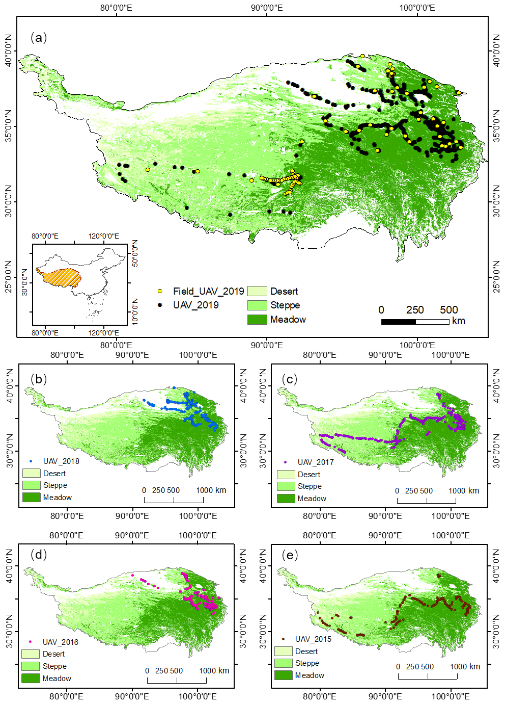
Figure 1Distribution of field and UAV sampling sites in 2019 (a). UAV sampling sites in grasslands on the QTP from 2015–2018 (b–e). Field_UAV_2019 represents the quadrat-scale sampling sites for the 2019 UAV field-synchronous grassland biomass experiment. UAV_year represents the UAV sampling points based on the GRID or RECTANGLE mode of the corresponding year.
2.1 Study site
The QTP is the highest and largest plateau on Earth (26∘00′12′′–39∘46′50′′ N, 73∘18′52′′–104∘46′59′′ E), with an average elevation of ∼4000 m and an area of approximately 257.24×10⁴ km2 (Fig. 1). It is located in western China, with an average annual temperature and precipitation of about 1.6 ∘C and 413.6 mm, respectively. The primary grassland types are meadow, steppe, and desert, which play a critical role in climate regulation, water conservation, and biodiversity protection (Ding et al., 2013). In this study, the boundary of the QTP (Zhang et al., 2014) was downloaded from the National Earth System Science Data Center, National Science and Technology Infrastructure of China (http://www.geodata.cn/, last access: 8 February 2023). Grassland types were derived from the 1:1 000 000 Chinese digital grassland classification map provided by the China Resource and Environmental Science Data Center (https://www.resdc.cn/, last access: 8 February 2023). This dataset, generated through field surveys in the 1980s and supplemented by satellite and aerial imagery, is the most detailed grassland-type map available. To facilitate comparison with other AGB estimates, we regrouped the grassland types into three categories, i.e., meadow, steppe, and desert (Table A1), and resampled this regrouped vector to a grid with 250 m spatial resolution.
2.2 Overall technology roadmap
The overall flowchart of this study is shown in Fig. 2. It consisted of four main steps, namely (1) UAV and field investigation, (2) constructing the AGB estimation model at the quadrat scale, (3) upscaling the grassland AGB to the MODIS pixel scale (250 m), and (4) building the AGB estimation model at the MODIS pixel scale (250 m) and applying it to the QTP region. More detailed information about each step was described in the following sections.
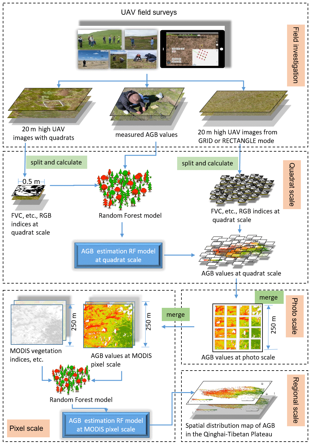
Figure 2The overall flowchart of UAV field survey and the construction of grassland AGB estimation models at different spatial scales.
2.3 Field investigation
2.3.1 UAV and route planning
DJI Phantom 3 Professional (SZ DJI Technology Co., Ltd., Shenzhen, China), a popular consumer quadrotor UAV with a high-resolution RGB (red, green, and blue) camera, was used to collect UAV photos of the QTP from 2015 to 2019. It has a in. (11.04 mm) CMOS sensor and is capable of taking 12 MP photos. In addition, it uses a three-axis stable gimbal to take photos vertically, downward, to eliminate the distortion of UAV photos. It has good environmental adaptability, with an operating temperature range from 0 to 40 ∘C, and a maximum takeoff altitude of 6000 m. Therefore, DJI Phantom 3 Professional is adequate to monitor grassland states on the QTP. More detailed information about the UAV system is listed in Table A2.
A fragmentation monitoring and analysis with aerial photography (FragMap) system was used for UAV route planning (Yi, 2017). During 2015–2019, we conducted UAV monitoring of the QTP grasslands using FragMap (Fig. 1). Over 2000 fixed flight routes were set up during this period, and more than 40 000 UAV photos were collected, providing a sufficient dataset for this study (Table 1).
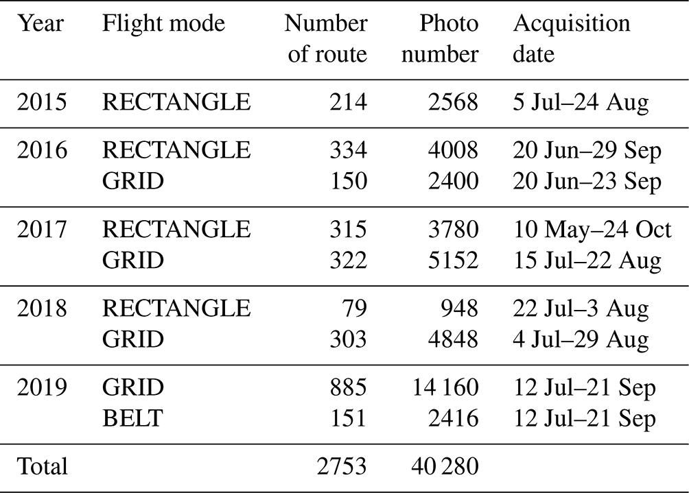
GRID, RECTANGLE, and BELT are the most widely used flight modes in FragMap software. Among these modes, GRID and RECTANGLE modes have 16 and 12 waypoints for capturing UAV photos within a MODIS pixel range (250 m × 250 m; Fig. A1). The flying height and speed are set to 20 m and 3 m s−1, respectively. The spatial coverage area of a 20 m high UAV photo is about 26 m × 35 m. The BELT mode is similar to GRID but is designed to obtain near-ground UAV photos with a higher resolution (Fig. 3b). Normally, the BELT size is set to 40 m × 40 m, and the flying height and speed are set to 2 m and 1 m s−1 to ensure that field crews have enough time to place sampling quadrats under the UAV waypoints. Therefore, it can be used to help field workers place sampling quadrats quickly and evenly. As with the GRID mode, 16 UAV photos can be captured in a single flight of BELT. Compared with the MOSAIC mode (which requires a guaranteed overlap rate between photos to obtain a full view of an area), our design is more in line with the traditional ecological sampling concept and more conducive to rapid sample collection.

Figure 3Schematic diagram of the UAV field synchronization experiment in 2019. A combination design of GRID (a) and BELT (b) flight modes. A UAV photo with a quadrat from the BELT mode at the height of 2 m (d). A 20 m high UAV photo including four sample quadrats (c). The cropped UAV photos at the quadrat scale from 20 m (e) and 2 m (f) height, respectively.
2.3.2 Synchronization experiment of UAV and field sampling
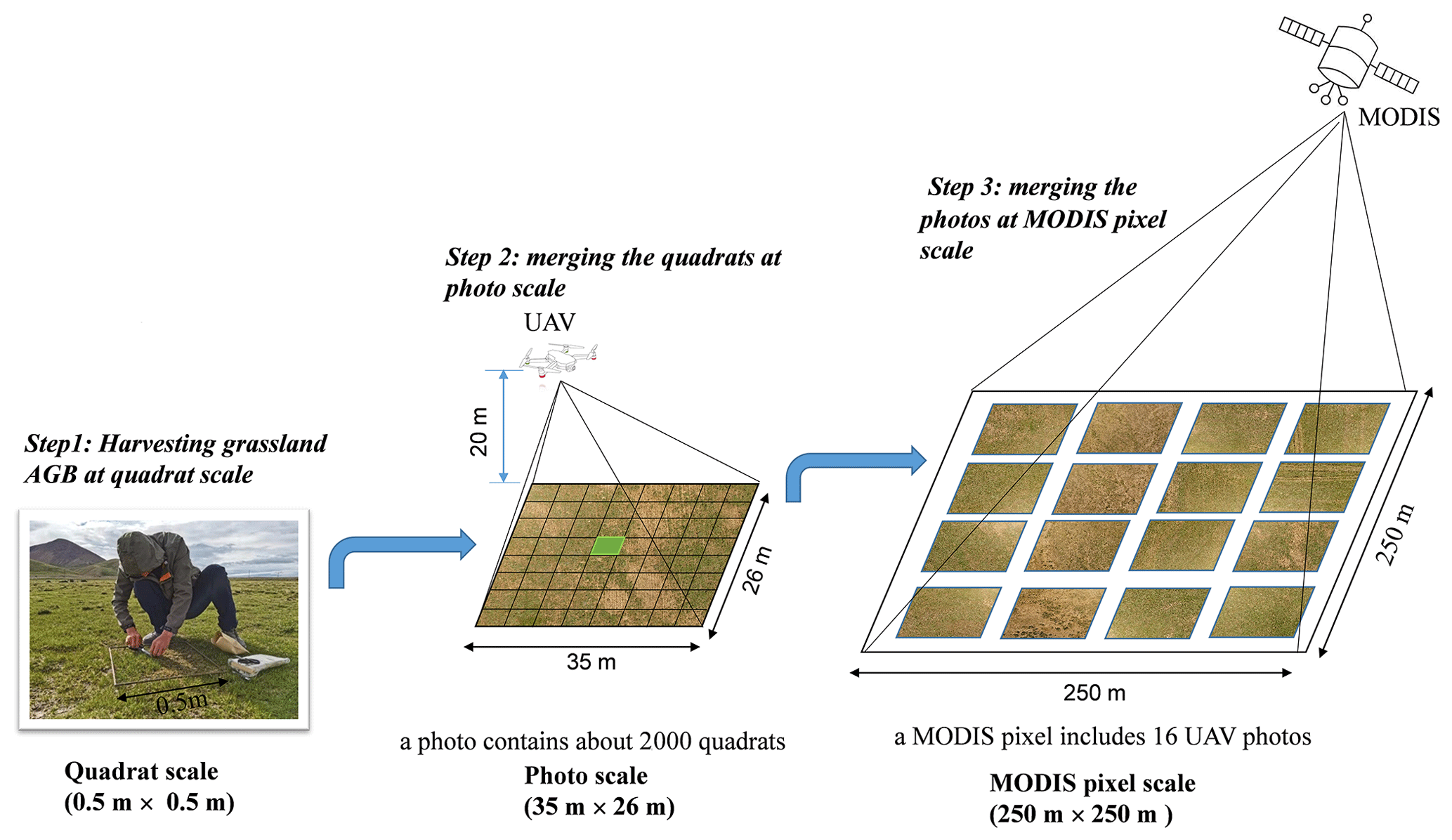
A UAV field biomass synchronization experiment was conducted in 2019 to ensure spatial matching among satellites, UAVs, and ground sampling (Fig. 3). The specific four steps were as follows. First, we set a GRID flight mode with a MODIS pixel size (250 m × 250 m; Fig. 3a). Second, three waypoints were selected from the GRID flight mode to set the BELT flight modes (40 m × 40 m). For each BELT, a sampling quadrat (0.5 m × 0.5 m) was placed at its 6, 7, 10, and 11 waypoints to ensure that the GRID photo could contain the four abovementioned quadrats (Fig. 3b and c). Third, after the implementation of all fights, the grassland samples were cut, bagged, and numbered. Finally, these samples were dried at 65 ∘C to a constant weight to obtain the AGB values measured in the field.
2.4 Data processing
2.4.1 UAV photo pre-processing and indices calculation
Pre-processing of UAV photos included image quality inspection, cropping, and calculation of different indices. It should be noted that only UAV photos at 20 m height were used in this paper. First, we eliminated overexposed or blurred 20 m high UAV photos. Second, the pixels in the sampling quadrats were cropped and saved (Fig. 3e). Third, the RGB indices, including color space, histogram, and vegetation indices, were calculated based on the method in our previous study (H. F. Zhang et al., 2022). In addition, 30 other RGB indices were added as candidate independent variables. The names, formulas, and references of the above indices are shown in Table A3.
2.4.2 MODIS vegetation index and other spatial data
The MOD13Q1 (v006) product was downloaded from the National Aeronautics and Space Administration (NASA) Earth Explorer website (https://earthexplorer.usgs.gov/, last access: 8 February 2023) for detecting the alpine grassland AGB on the QTP. The data contained two commonly used vegetation indices, i.e., the normalized difference vegetation index (NDVI) and the enhanced vegetation index (EVI), with spatial and temporal resolutions of 250 m and 16 d, respectively. A total of 2842 scenes from 2000 to 2019 were downloaded. Then, the MODIS images were reprojected and mosaicked using the MODIS Reprojection Tool (MRT). After that, the corresponding vegetation indices closest to the date of the UAV sampling were extracted to construct/validate the MODIS pixel-scale AGB estimation model. In addition, the kernel normalized difference vegetation index (kNDVI) was calculated to overcome the NDVI saturation issue based on the equation kNDVI = TANH (NDVI2) (Camps-Valls et al., 2021). The annual maximum vegetation indices were calculated by the maximum-value composition (MVC) algorithm to estimate the spatial AGB distribution of the QTP from 2000 to 2019 (Holben, 1986; Wang et al., 2021; Gao et al., 2020).
Furthermore, meteorological, soil texture, and topographic data were included as candidate-independent variables for constructing the MODIS pixel-scale AGB estimation model. Meteorological factors, including mean annual temperature (MAT), mean annual precipitation (MAP), and total annual solar radiation (TASR), were calculated based on the daily meteorological dataset from the China Meteorological Data Service Centre (http://data.cma.cn/, last access: 8 February 2023). The data-processing steps mainly included checking and eliminating the anomalous values of attributes, cumulative summation, annual averaging, and interpolation to obtain a meteorological raster dataset with a spatial resolution of 1 km (Li et al., 2021). Moreover, soil texture data at 1 km spatial resolution, including the ratio of soil organic matter (SOM), clay, sand, and silt, were downloaded from the Resources and Environmental Science Data Center of China (https://www.resdc.cn/, last access: 8 February 2023). All the meteorological and soil raster datasets were regridded into 250 m by ArcGIS software (version 10.2; Environmental Systems Research Institute, Inc.) to match the MODIS image.
Terrain factors including altitude, slope, and aspect were derived from the digital elevation model (DEM) using the terrain analysis tool of ArcGIS software. The DEM was retrieved from Shuttle Radar Topography Mission (SRTM) imagery (version 004; 90 m) and regridded to 250 m.
2.5 AGB modeling and computation at different scales
We estimated the grassland AGB at three scales, namely the quadrat scale, the photo scale, and the MODIS pixel scale (Fig. 4). More detailed information was described as follows.
2.5.1 Random forest model
Random forest (RF; Breiman, 2001) is an ensemble-learning algorithm that has been widely used to estimate AGB due to its excellent performance (Ghosh and Behera, 2018; Mutanga et al., 2012; Wang et al., 2016). The two primary parameters, named the number of regression trees in the forest (ntree) and the number of feature variables required to create branches (mtry), were firstly optimized based on the root mean square error (RMSE) of training data. Here, the value of ntree was set from 100 to 5000, with an interval of 100, while mtry was set as the square root of the number of training sample features. In addition, the importance of each predictor was ranked by calculating the percentage increased in mean square error (% IncMSE).
The backward feature elimination method (BFE) was used to reduce the number of input variables to simplify the RF model (Vergara and Estévez, 2014). The primary steps were as follows: (1) constructing an AGB RF model by including all predictors in the initial stages and calculating the % IncMSE for each variable and (2) eliminating the least-promising variable and then rerunning the RF model until only one independent variable was left. Moreover, the corresponding coefficient of determination (R2) and the corresponding RMSE were calculated in each iteration; (3) the smallest subset of variables with the highest R2 was selected as the final optimized indices.
In addition, different training and validation strategies were used at different scales. Due to the limited ground samples, a 10-fold cross-validation method was used at the quadrat scale (Kohavi, 1995). At the MODIS pixel scale, 30 % of the UAV-estimated AGB samples in 2019 were randomly selected as an independent validation dataset due to the large size. Meanwhile, the UAV_AGB values from 2015 to 2018 were used for multi-year validation to test the robustness of the model over time. Statistical metrics R2 (Eq. 1) and RMSE (Eq. 2) were used to evaluate model performance.
where n is the number of samples, yi and represent the measured and the predicted AGB value, respectively, and is the mean value of measured AGB samples.
2.5.2 AGB RF estimation model at the quadrat scale (0.25 m2)
Since the spatial coverage area of a 20 m high UAV photo (26 m × 35 m) is much larger than a single 2 m high UAV photo (0.8 m × 1 m), it is easier to match the MODIS pixel scale (250 m × 250 m). Hence, the 20 m high UAV photos containing the sample quadrats were chosen for constructing the quadrat-scale AGB estimation model. A total of 906 pairs between field-harvested AGB and UAV sub-photos were collected, with good spatial representativeness (Fig. 1a; yellow dots). The observed AGB values ranged from 0 to 450 g m−2, with mean and median values of 59.75 and 33.04 g m−2, respectively (Fig. 5a). The cropped 20 m high UAV photo indices and the measured AGB values were used as the independent and dependent variables to build the RF model at the quadrat scale (Fig. 2).
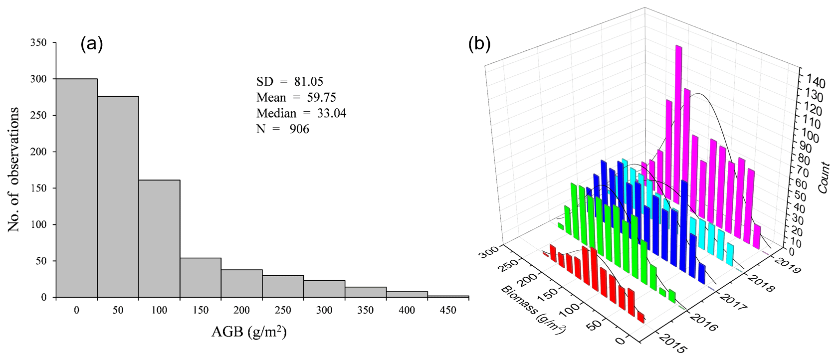
Figure 5Histograms of field-measured AGB values at quadrat scale (a) and UAV-estimated AGB values of different years at the photo scale (b).
2.5.3 AGB calculation at the photo scale (∼900 m2)
The steps for AGB estimation of the whole 20 m high UAV photo were as follows: (1) first, each UAV photo was split into ∼2000 quadrat-sized small patches. (2) Second, the AGB of each small patch was calculated based on the quadrat-scale AGB estimation model. (3) Finally, the average of all small patches was calculated as the AGB of the whole photo. Based on the above steps, the AGB values of more than 75×106 quadrats in 37 864 photos in GRID or RECTANGLE mode were calculated (Table 1).
Table 2Selected independent variables for the AGB modeling at quadrat and pixel scales. The full names of each variable at the quadrat scale are listed in Table A3.

2.5.4 AGB RF model construction at MODIS pixel scale (62 500 m2)
The following steps were involved in constructing the AGB estimation model at the MODIS pixel scale. (1) Since the coverage area of a GRID or RECTANGLE mode was similar to that of a MODIS pixel, the average value of the AGB of 16 or 12 UAV photos was taken as the AGB value of the corresponding MODIS pixel. During 2015–2019, a total of 2602 UAV-estimated AGB samples were obtained at the MODIS pixel scale (Table 1). (2) The MODIS vegetation indices and other spatial metrics (such as meteorological, soil texture, and topographic data) corresponding to each GRID or RECTANGLE mode were then extracted using the ArcGIS software. Here, the MODIS NDVI, EVI, and kNDVI indices closest to the sampling date were chosen to minimize the time difference between sampling and satellite overpass. (3) Subsequently, the UAV-estimated AGB values, MODIS vegetation indices, and other spatial metrics were used as dependent and independent variables to build the AGB-estimated model at MODIS pixel scale using the RF model.
2.6 Uncertainty analysis
Since the actual AGB values of MODIS pixels cannot be directly obtained, the regression coefficient between vegetation indices and estimated AGB was used to quantify the uncertainty in different AGB estimation methods. In other words, the higher the correlation between the estimated AGB and MODIS vegetation indices, the more accurate the estimation model was. The performance of the estimation model was evaluated through three aspects. In this study, we first compared the correlation between the MODIS vegetation indices and AGB values obtained by traditional sampling and UAV estimation methods. We also explored the uncertainties in UAV sampling coverage area by regularly combining the number of photos in a MODIS pixel and tested whether the estimated AGB was closer to the “true” value as the number increased. Furthermore, the AGB validation results between GRID and RECTANGLE at the pixel scale were compared to understand the uncertainties caused by different flight modes.
2.7 Trend analysis of grassland AGB
This study combined the Theil–Sen median trend analysis and Mann–Kendall test to analyze the temporal variation characteristics of grassland AGB in the QTP (Jiang et al., 2015). The Theil–Sen median trend analysis is a robust trend statistical method with high computational efficiency that is insensitive to outliers (Hoaglin et al., 1983). The Mann–Kendall test is a nonparametric test for time series trends, which does not require the measurements to follow a normal distribution, and is not affected by missing values and outliers. The Theil–Sen Median trend analysis and Mann–Kendall trend test have been widely used to analyze the temporal trends of the vegetation index, cover, and biomass (Gao et al., 2020; Jiang et al., 2015; Fensholt et al., 2009). The detailed formulas for the Theil–Sen median trend analysis and the Mann–Kendall method are provided by Jiang et al. (2015).
Table 3Validation results of AGB models at the quadrat and pixel scales.

Values significant at p<0.001.
3.1 Independent variables selected for AGB modeling
The independent variables for AGB estimation at the quadrat and MODIS pixel scales are presented in Table 2. A total of 36 independent variables were selected at the quadrat scale, including 26 vegetation RGB indices, 6 histogram indices, and 4 color space indices (Fig. A2). At the MODIS pixel scale, five variables were selected, including NDVI, kNDVI, EVI, MAP, and DEM (Fig. A3).
Table 4T test results between the predicted and measured AGB values for the modes at the quadrat and pixel scales. Note that df means degrees of freedom.

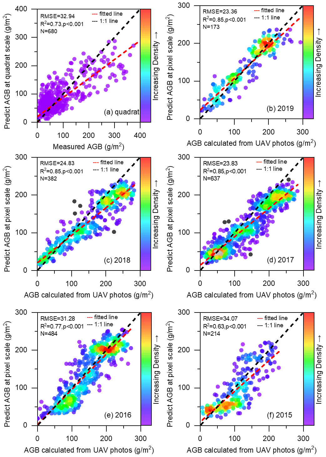
Figure 6Validation results of the AGB estimation models at the quadrat (a) and MODIS pixel scale for 2015–2019 (b–f).
3.2 Modeling and accuracy assessment
For the AGB estimation model at the quadrat scale, the results of 10 cross-validations showed that there was a significant linear relationship between the estimated and the field-measured values (R2=0.73; p<0.001; Tables 3 and A4). There was no significant difference (p>0.05) between the predicted and the measured values of the mean AGB, at a confidence level of 95 % (Table 4), with an RMSE of 32.94 g m−2 (Table 3). The model predicted well when the measured biomass was less than 150 g m−2; however, underestimation was found when the measured biomass was more than 200 g m−2 (Fig. 6a). It may be because the number of samples of more than 200 g m−2 is relatively small, accounting for only 8.50 % of all samples (Fig. 5a). Although the sample amount of the UAV varied year by year, the AGB values estimated from UAV photos typically ranged from 0 to 300 g m−2 (Fig. 5b).
For the AGB estimation model at the MODIS pixel scale, there was a strong linear relationship (p<0.05) between the estimated AGB and that measured by UAV photos for 2015–2019 (Table A4). The fitting coefficient R2 was 0.85 for 2017–2019 and slightly lower for 2015–2016, with the values of 0.63 and 0.77, respectively (Table 3, Fig. 6b–f). The RMSE of the MODIS pixel-scale model ranged from 23.36 to 34.07 g m−2 (Table 3). In addition, we found no significant differences (p>0.05) between the predicted and measured values of the average AGB, except for 2017 and 2018 (Table 4). The average AGB estimated by the MODIS pixel-scale model for 2017 and 2018 was 131.48 and 120.60 g m−2, which were 14.72 % and 13.78 % lower than those estimated by UAV photos. Although the average AGB estimates between the MODIS pixel-scale model and UAV were different in 2017 and 2018, the error percentages were acceptable. Therefore, the constructed MODIS pixel-scale AGB estimation model had good performance and robustness in different years (Fig. 6b–f).
3.3 Correlation analysis between AGB values and MODIS indices
The correlations between the UAV-estimated AGB and MODIS vegetation indices were much better than those between field-harvested AGB and MODIS vegetation indices (Fig. 7a). For example, the correlation between NDVI and field-harvested AGB was only 0.53, which is considerably lower than the correlation between NDVI and AGB obtained from a single UAV photo (R=0.74). Moreover, the correlation between NDVI and UAV-estimated AGB increased with the increasing number of UAV photos. It increased rapidly as the number of UAV photos increased from 1 to 4 (from 0.74 to 0.86) and then slowed down and stabilized (from 0.87 to 0.88). In addition, we compared the scatterplots and fitting lines between NDVI and different AGB estimation methods (Fig. 7b–f). The results showed a weak linear relationship between the field-measured AGB and NDVI, with an R2 of 0.29. While using the UAV sampling method, the linear relationship was greatly improved and increased with the increasing number of photos. The fit coefficient R2 increased from 0.54 to 0.78, which is much higher than the traditional sampling method (Fig. 7).
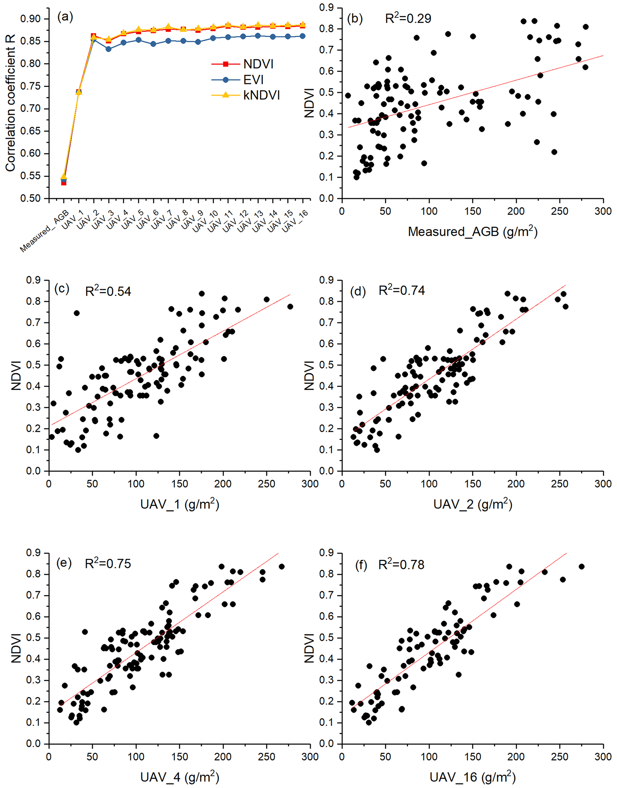
Figure 7Correlation between MODIS vegetation indices and different AGB estimation methods (a). Scatterplots of NDVI with different AGB estimation methods (b–f). UAV_x represents the number of UAV photos used to estimate the average AGB at the MODIS pixel scale. Here, x ranges from 1 to 16.
3.4 Spatial distribution of grassland AGB
The spatial distribution of the average grassland AGB on the QTP from 2000 to 2019 was calculated (Fig. 8). The AGB gradually increased from west to east. The average AGB of eastern OA1, IIAB1, IB1, and IIC2 (see Table A5 for the full definitions of these and other abbreviations) eco-geographical regions ranged from 150 to 190 g m−2, and the average AGB of IC1 and IIC1 ranged from 80 to 110 g m−2 (Fig. 8b). The average AGB of IID2, IID3, IC2, and IID1 in the west was relatively low, ranging from 35 to 75 g m−2. The ID1 region was dominated by desert grassland with the lowest average annual AGB values, which fluctuated around 20 g m−2 (Fig. 8b). Except for the low AGB due to low precipitation in 2015 (Fig. A4), the mean AGB showed an overall increasing trend from 2000 to 2019, with an average growth rate of 0.22 g m−2 a−1 (Fig. 9a). The overall mean AGB of the QTP was 103.6 g m−2, with 151.85, 60.85, and 28.91 g m−2 for meadow, steppe, and desert grassland, respectively (Fig. 9b). In addition, the temporal trend of grassland AGB in each pixel was analyzed. As shown in Fig. 10, the IID3, ID1, IID2, and IIC2 eco-geographical regions of the northern QTP showed an increasing trend from 2000 to 2019, while the IC2, IB1, and IIC1 regions showed a decreasing trend. Therefore, there was spatial heterogeneity in the temporal variation.
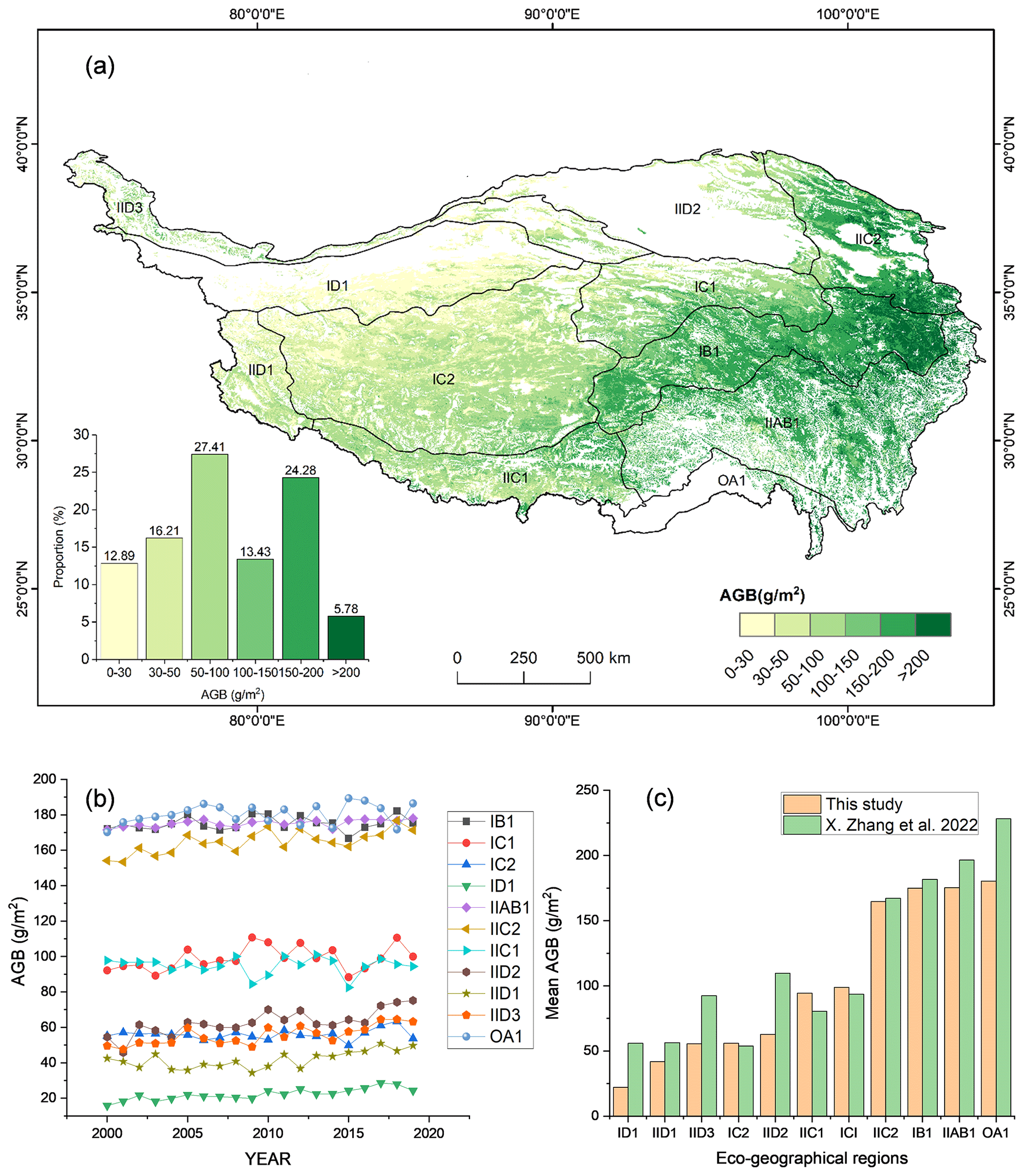
Figure 8(a) The spatial distribution of average grassland AGB on the QTP from 2000 to 2019. IID1, IID2, IID3, ID, IIC1, IIC2, IC1, IB1 IIAB1, and OA1 are the eco-geographical regions of the QTP (Zheng, 1996). The full names of each eco-geographical region are listed in Table A5. (b) AGB values of each eco-geographical region from 2000 to 2019. (c) Comparison of multi-year AGB averages in the different eco-geographical regions.
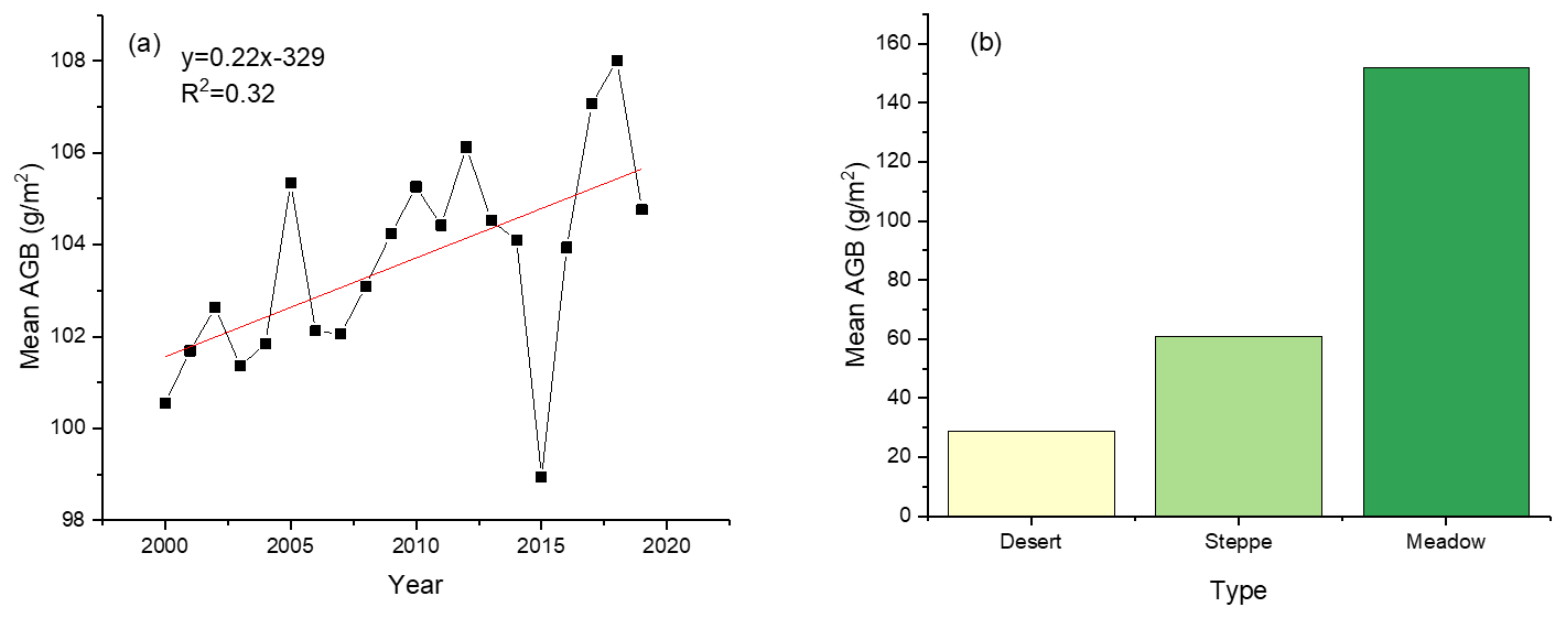
Figure 9Variation trend for average grassland AGB on the QTP from 2000 to 2019 (a) and the average AGB of different grassland types (b).

Figure 10Spatial trends of grassland AGB on the QTP from 2000 to 2019. IID1, IID2, IID3, ID, IIC1, IIC2, IC1, IB1 IIAB1, and OA1 are the eco-geographical regions of the QTP (Zheng, 1996). The full names of each eco-geographical region are listed in Table A5.
4.1 Scale matching and its impact factor
In previous studies, the AGB values at the satellite pixel scale were usually represented by the average of 3–5 quadrat-scale samples placed in the corresponding satellite pixel, resulting in a large spatial gap between the ground samples and the satellite pixels (Yang et al., 2009, 2018; Meng et al., 2020). The spatial gap between ground samples and satellite pixels affects the accuracy of grassland AGB estimation models (Morais et al., 2021). Therefore, we used the UAVs as a bridge to fill the spatial gap. Spatial-scale matching of dependent and independent variables was achieved by estimating AGB values at different scales. First, at the quadrat scale, the independent variables were all derived from cropped 20 m high UAV photos corresponding to the ground samples (Fig. 3e). Second, the 20 m high UAV photo was split into ∼2000 quadrat-sized patches to ensure consistency with the quadrat-scale model, and the average of these patches was used as the final AGB at the photo scale. Finally, the AGB matching the MODIS pixel scale was calculated by averaging the AGB of 16 or 12 UAV photos within the MODIS pixel (Fig. A1). With these three steps, we successfully upscaled the measured AGB from quadrat scale (0.5 m × 0.5 m) to photo scale (26 m × 35 m) and MODIS pixel scale (250 m × 250 m). Our results showed that the correlations between the UAV-estimated AGB values and the MODIS vegetation indices were higher than that between field-harvested AGB and MODIS vegetation indices (Fig. 7).
Furthermore, we found that the spatial coverage area of the UAV sampling had an impact on the scale matching. Our results showed that, the closer the spatial coverage area of the UAV sampling was to the satellite pixel, the higher its correlation with MODIS vegetation indices (Fig. 7a). It was further confirmed by comparing the validation results of different flight modes. At the MODIS pixel scale, we found that the R2 between the model predictions and the AGB values estimated by GRID mode was better than that of the RECTANGLE mode (Fig. 11). The reason is that GRID mode can take 16 photos within a MODIS pixel, while RECTANGLE mode can only take 12 photos (Fig. A1). As a result, UAV photos could serve as a bridge to effectively fill the spatial gap between traditional samples and satellite data.
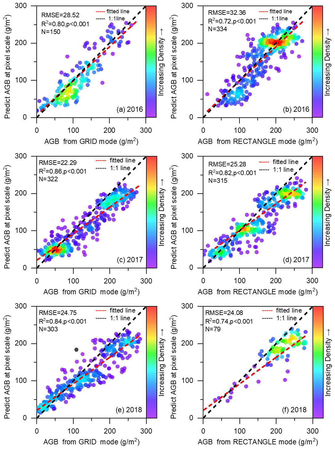
Figure 11Comparison of the validation results for the GRID (a, c, e) and RECTANGLE (b, d, f) modes in 2016–2018.
4.2 Importance of the addition of non-vegetation samples
Compared with traditional sampling (Yang et al., 2018), UAV sampling has the advantage of larger spatial coverage area (0.5 m × 0.5 m vs. 35 m × 26 m). Thus, the UAV photo could capture non-vegetation background information such as roads, water, soil, gravel, and riverbed (Fig. A5). Adding non-vegetation samples could improve the accuracy of AGB estimation at the photo scale, especially for areas with low vegetation cover. It was also suitable for the pixel-scale AGB estimation model.
4.3 Comparison of the estimated AGB with previous studies
We compared our results with previous studies at the quadrat, pixel, and regional scales. At the quadrat scale, consistent with our previous study, we further confirmed that the UAV photos could be used to estimate grassland AGB (H. F. Zhang et al., 2022; Zhang et al., 2018). Similar to the 2 m high UAV photo, the 20 m high UAV photo could be used to estimate the grassland AGB at the quadrat scale (R2=0.73; RMSE = 44.23 g m−2; Fig. 6a). Compared with the 2 m high UAV photo (0.8 m × 1 m), the 20 m high UAV photo (26 m × 35 m) is more suitable for matching the MODIS pixel due to its larger spatial coverage area. In addition, the direct use of the 20 m high photo eliminates the need for spatial-scale conversions when upscaling the AGB estimation from the quadrat scale to the photo scale.
At the pixel scale, compared with other studies, this paper achieved the spatial-scale matching of independent and dependent variables during the modeling. In previous studies (Yang et al., 2009, 2018; Meng et al., 2020), they constructed the models from the measured AGB values at the quadrat scale and the spectral indices of the satellites without considering the spatial-scale difference. It partly explained why the R2 of the AGB linear model constructed by Yang et al. (2009) was only 0.4. Our results confirmed that the R2 of the linear model could be increased from 0.29 to 0.78 after filling the spatial gap between measured AGB and MODIS NDVI (Fig. 7). In addition, thanks to the rapid sampling of UAV technology, a total of 2602 UAV samples matching the MODIS pixel scale were collected during 2015–2019. It allowed us to perform multi-year validation to assess the robustness of the model over time, which has rarely been performed in previous studies. Our results showed similar validation results for 2017–2019, despite different sample amounts and spatial distributions (Fig. 1; Table 1). But in 2015–2016, R2 was relatively low, at 0.63 and 0.77, respectively (Table 3, Fig. 6). The reason was that, during 2015–2016, some photos with unnatural white balance were obtained due to improper settings, which reduced the estimation accuracy (Fig. A6). The validation results showed that the MODIS pixel-scale AGB estimation model had good robustness in different regions and times whenever the photo quality was acceptable.
Table 5Comparison of AGB estimation results of different studies on the QTP.

At the regional scale, consistent with previous results, we found an overall increase in AGB over the QTP from 2000 to 2019, albeit with fluctuations (Zeng et al., 2019; Gao et al., 2020). The annual average AGB of grassland was 103.6 g m−2, which was closest to X. Zhang et al. (2022) and within the range of the previous estimates (59.63–120.73 g m−2; Table 5). The mean AGB varied among different grassland types, with 151.85 g m−2 for the meadow and 60.85 g m−2 for the steppe. Our estimation results were similar to those of Zeng et al. (2019), but the overall average AGB was higher than their estimate of 77.12 g m−2. The spatial distribution of AGB was consistent with previous studies, showing a west-to-east increasing trend (X. Zhang et al., 2022; Xia et al., 2018). Specifically, the average AGB of OA1, IIAB1, IB1, and IIC2 eco-geographical regions in the east was significantly higher than that of IID2, IID3, IC2, IID1, and ID1 regions in the west (Fig. 8). In general, the average AGB estimates for each eco-geographical region in this paper were similar to those reported by X. Zhang et al. (2022). Among them, our average AGB estimates for ID1, IID1, IID3, and IID2 regions were slightly lower, but our values were closer to the measured values of these regions (Fig. 8c). The reason may be that they calculated the potential AGB, while we calculated the actual AGB, so our estimate was relatively low. In terms of spatial and temporal trends, the data results showed that the eco-geographical regions in the northern part of the QTP demonstrated an increasing trend (IID3, ID1, IID2, and IIC2), while the IC2, IIC1, and IB1 regions exhibited a significant or non-significant decrease, which was consistent with the results of others (Gao et al., 2020; Liu et al., 2017).
The difference between our estimated grassland AGB and previous studies might be due to differences in data sources and modeling methods. First, the sample amount and spatial distribution of ground samples were different. The number of ground samples is the most important variable affecting the accuracy of the grassland AGB estimation model (Morais et al., 2021). Unlike previous studies, we collected ground validation data by combining the traditional sampling method and UAVs. The newly proposed method could overcome the shortcomings of traditional samplings (time-consuming and labor intensive). It no longer takes years to obtain spatially representative, large-scale ground validation data (Yang et al., 2018). With UAV sampling, ground observations matching the satellite pixel scale can be obtained in only 15–20 min, which is difficult to achieve with traditional surveys. Our new sampling method not only accelerates the sampling speed and increases the sample amount but also improves the spatial match between ground samples and satellite pixels. As a result, our ground validation data is better than previous studies in terms of quantity and spatial-scale matching with the satellite data. Second, the input parameters of AGB estimation models were different. Some scholars used only a single vegetation index (NDVI or EVI), while others combined the vegetation index with meteorological, soil, and terrain indices to construct the AGB estimation models (Table 5). In this study, NDVI, kNDVI, EVI, DEM, and MAP were used as the final predictor variables to construct the AGB estimation model at the MODIS pixel scale (Table 2). Third, modeling methods might also affect the estimation results. As shown in Table 5, the overall AGB averages of the QTP estimated based on different methods (such as linear or nonlinear regression, machine learning, and ecological process model methods) varied considerably. Yang et al. (2018) found that the model performance of the artificial neural network (ANN) was much better than the linear regression model when using the same dataset to estimate grassland AGB in the three-rivers headwaters region of China. Jia et al. (2016) reported that the model forms could bring 13 % uncertainty to the AGB estimation. Wang et al. (2017) compared the RF with the bagging, mboost, and support vector regression (SVR) algorithms and found that the RF yielded the best performance in grassland AGB estimation.
4.4 Limitations and further work
We acknowledge that there are some shortcomings in this study. (1) The predicted values of the quadrat-scale model were underestimated when the measured biomass values were greater than 250 g m−2 (Fig. 6). One of the reasons may be that the number of samples larger than 250 g m−2 at the quadrat scale is relatively small, accounting for only 5.18 % of the total samples. Another possible reason is that the height of the grassland could not be detected by a single UAV photo. Therefore, it could lead to an underestimation of AGB for grassland species with the same FVC but greater heights. Previous studies have shown that adding vegetation height information can improve the estimation accuracy of grassland AGB (H. F. Zhang et al., 2022; Lussem et al., 2019; Viljanen et al., 2018). In future work, an affordable DJI ZENMUSE L1 scanner mounted on the UAV DJI Matrice 300 will be introduced to detect the height of the grassland. (2) At the MODIS pixel scale, limited by the estimation accuracy of AGB from UAV photos, there was also some underestimation in the high biomass area. Although the MODIS indices closest to the sampling date were chosen for the construction/validation of the AGB estimation model, there was still a time gap between the measured samples and the MODIS indices, which might lead to estimation uncertainties. In addition, the NDVI saturation problem was not considered in this study, which might affect the AGB estimation accuracy in the QTP (Tucker, 1979; Gao et al., 2000; Mutanga and Skidmore, 2004). In the next step, we will continue to collect samples with high biomass and try to correct the NDVI saturation problem for optimizing the simulation accuracy of the dataset. (3) During 2015–2016, we set the automatic white balance mode for UAV shooting due to inexperience. As a result, some photos with unnatural white balance were obtained, reducing the accuracy of AGB estimation at the photo scale (Fig. A6). (4) We collected grassland AGB only during the peak growing season, and the applicability of the proposed method to other growing seasons needs further study. (5) During the modeling process, due to the poor positioning accuracy, only the center points of the flight path were used to find the corresponding MODIS pixels. Moreover, although the UAV photos in the GRID or RECTANGLE mode could cover most areas of a MODIS pixel, full-pixel coverage was still not achieved. Therefore, we will gradually upscale to MODIS pixels by combining UAVs with Sentinel-2 or Landsat images.
The dataset is available from the National Tibetan Plateau/Third Pole Environment Data Center (https://doi.org/10.11888/Terre.tpdc.272587; H. Zhang et al., 2022). The dataset contains 20 years of AGB spatial data of the QTP with a resolution of 250 m and is stored in TIFF format. The name of the file is “AGB_yyyy.tif”, where yyyy represents the year. For example, AGB_2000.tif represents this TIFF file describing the alpine grassland AGB condition of QTP in 2000. The data can be readily imported into standard geographical information system software (e.g., ArcGIS) or accessed in a programmatic manner (e.g., MATLAB and Python).
This study developed a new AGB dataset for alpine grasslands on the QTP based on traditional ground sampling, UAV photography, and MODIS imagery. The uniqueness of this dataset is the use of UAVs as a spatial-scale-matching bridge between traditional samples and MODIS pixels. The study confirmed that UAV photos could be used for AGB estimation at the quadrat/MODIS pixel scale, with R2 of 0.73/0.83 and RMSE of 44.23/34.13 g m−2, respectively. At the MODIS pixel scale, the correlations between AGB estimated by UAV and MODIS vegetation indices were higher than that between field-harvested AGB and MODIS vegetation indices. Moreover, the spatial-scale matching of the dependent and the independent variables was achieved during the modeling. In addition, we performed a multi-year validation of the MODIS pixel-scale AGB estimation model to confirm the robustness of the model and the accuracy of this dataset. The availability of the new dataset is helpful in many applications. First, this dataset provides reliable regional data for estimating grassland productivity, carbon storage, ecological carrying capacity, and ecological service functions (such as feed for grazing livestock) of the QTP. Second, the dataset can be used to understand the mechanisms of environmental processes, such as hydrological cycle processes, soil erosion and degradation, and carbon cycle processes in the QTP. In addition, this dataset can be used as input or validation parameters for various ecological models to understand the response mechanism of the QTP to global climate change.
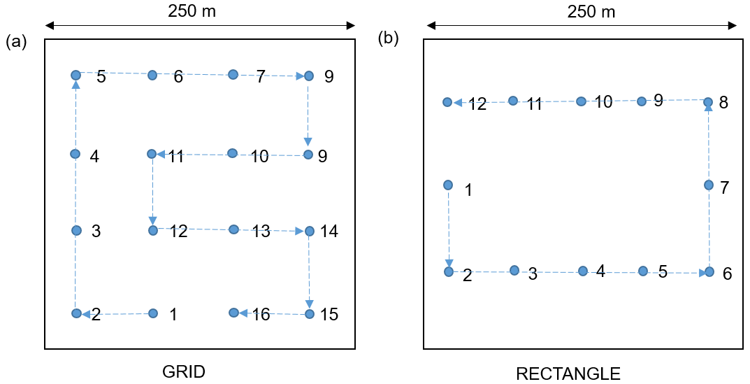
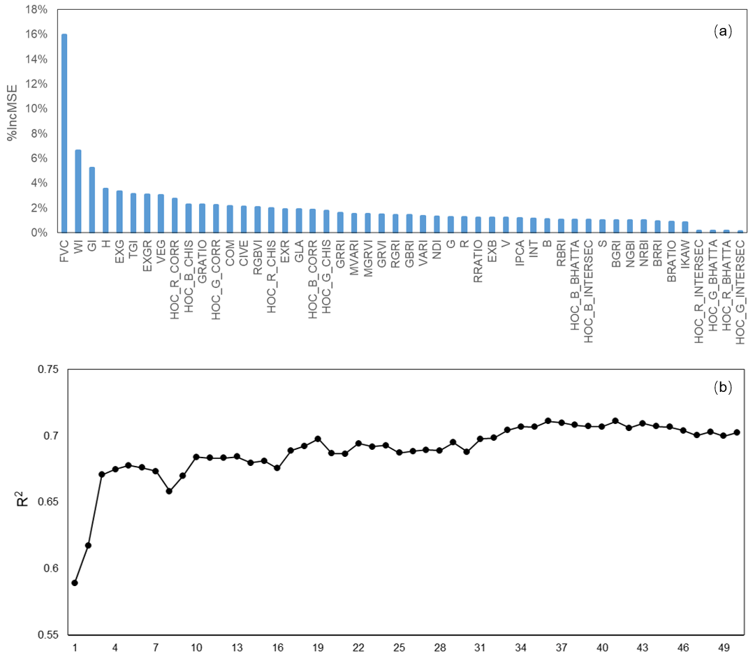
Figure A2The important values for each independent variable (a) and the R2 results of the different number of input variables at the quadrat scale (b).

Figure A3The important values for each independent variable (a) and the R2 results of the different number of input variables at the MODIS pixel scale (b).
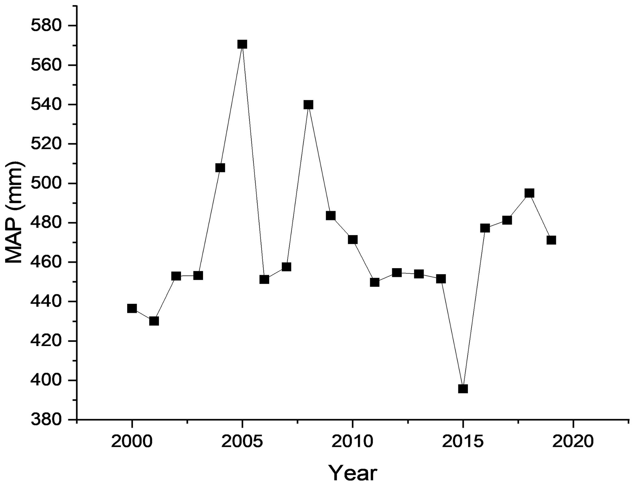
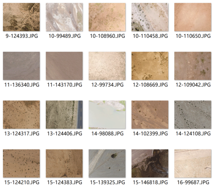
Figure A5Examples of 20 m high UAV photos with different non-vegetation background information.
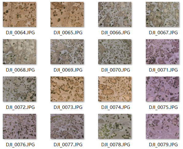
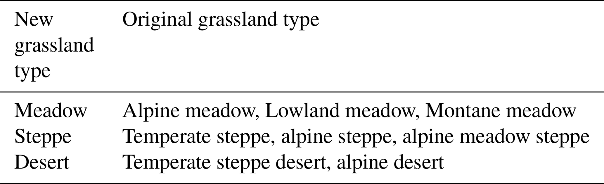
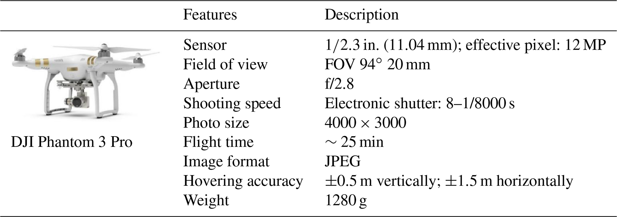
Table A3Details of the independent variables for quadrat-scale AGB estimation. Note that HSV is for hue, saturation, and value.
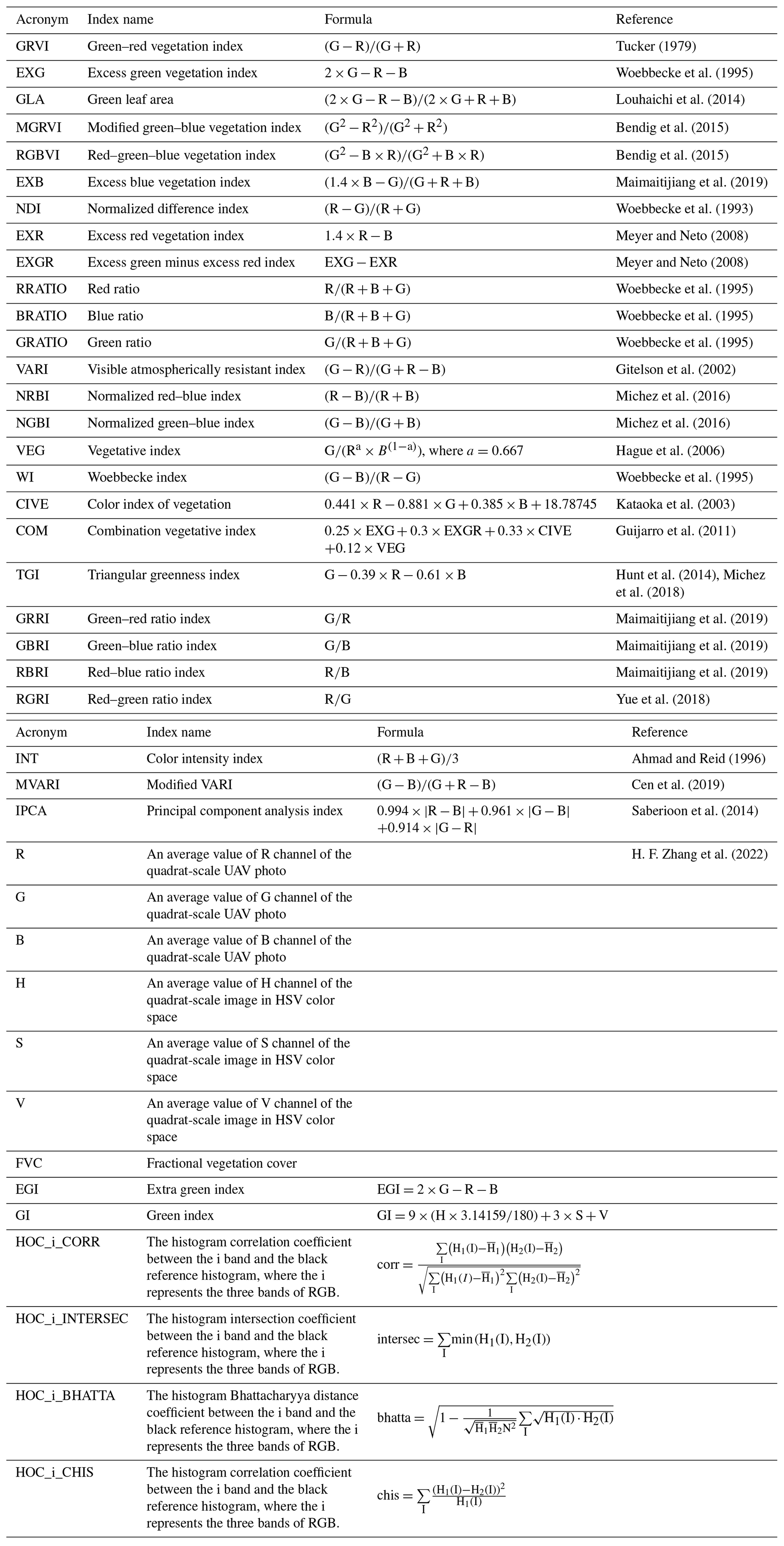
Table A4Regression analysis for AGB estimation models at quadrat and pixel scales.
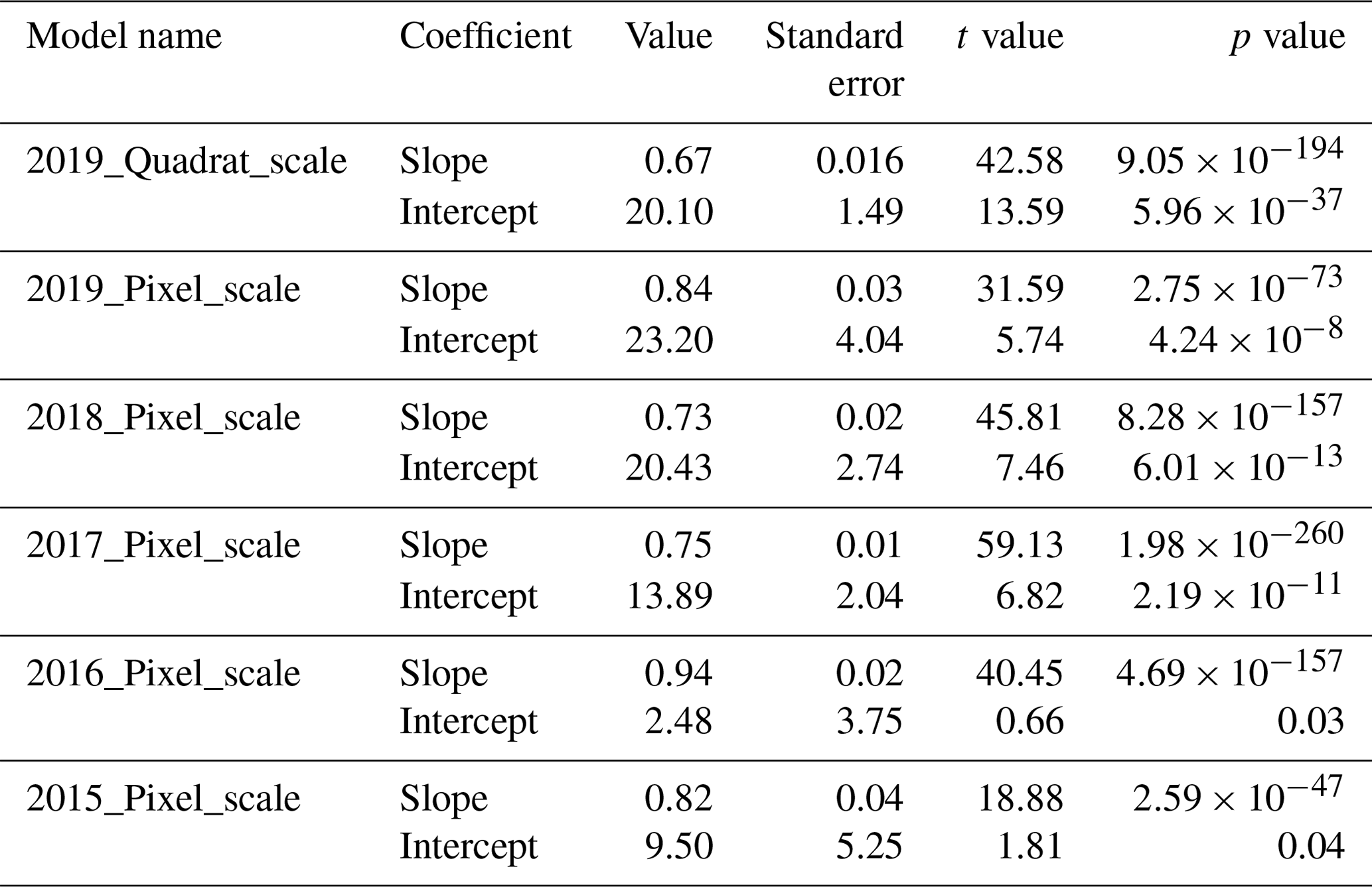
Table A5List of abbreviations of eco-geographical regions of the QTP.

HZ contributed to the study conceptualization, methodology, funding acquisition, and the original draft. ZT, BW, and HK contributed to resources and formal analysis. YQ and YS contributed to data collection and review of the paper. BM, ML, and JC contributed to the methodology and reviewed the paper. YL and JZ participated in reviewing and editing the paper. SN contributed to the data collection and review of the paper. SY contributed to the study conceptualization, funding acquisition, and the paper review. All authors have read and approved the paper.
The contact author has declared that none of the authors has any competing interests.
Publisher's note: Copernicus Publications remains neutral with regard to jurisdictional claims in published maps and institutional affiliations.
This article is part of the special issue “Extreme environment datasets for the three poles”. It is not associated with a conference.
We would like to express our gratitude to the other students and staff, who participated in the field investigation. We are grateful to the anonymous reviewers, who also contributed greatly to the improvement of an earlier version of this paper.
This research has been supported by the National Natural Science Foundation of China (grant no. 41801023), the National Key R & D Program of China (grant no. 2017YFA0604801), and the National Natural Science Foundation of China (grant no. 42071056).
This paper was edited by Min Feng and reviewed by Jinhu Bian and two anonymous referees.
Ahmad, I. S. and Reid, J. F.: Evaluation of Colour Representations for Maize Images, J. Agric. Eng. Res., 63, 185–195, https://doi.org/10.1006/jaer.1996.0020, 1996.
Bendig, J., Yu, K., Aasen, H., Bolten, A., Bennertz, S., Broscheit, J., Gnyp, M. L., and Bareth, G.: Combining UAV-based plant height from crop surface models, visible, and near infrared vegetation indices for biomass monitoring in barley, Int. J. Appl. Earth Obs. Geoinf., 39, 79–87, https://doi.org/10.1016/j.jag.2015.02.012, 2015.
Bian, L. and Walsh, S. J.: Scale dependencies of vegetation and topography in a mountainous environment of Montana, Prof. Geogr., 45, 1–11, https://doi.org/10.1111/j.0033-0124.1993.00001.x, 1993.
Breiman, L.: Random forests, Mach. Learn., 45, 5–32, https://doi.org/10.1023/A:1010933404324, 2001.
Camps-Valls, G., Campos-Taberner, M., Moreno-Martinez, A., Walther, S., Duveiller, G., Cescatti, A., Mahecha, M. D., Munoz-Mari, J., Garcia-Haro, F. J., Guanter, L., Jung, M., Gamon, J. A., Reichstein, M., and Running, S. W.: A unified vegetation index for quantifying the terrestrial biosphere, Sci. Adv., 7, eabc7447, https://doi.org/10.1126/sciadv.abc7447, 2021.
Cannavacciuolo, M., Bellido, A., Cluzeau, D., Gascuel, C., and Trehen, P.: A geostatistical approach to the study of earthworm distribution in grassland, Appl. Soil Ecol., 9, 345–349, https://doi.org/10.1016/S0929-1393(98)00087-0, 1998.
Cen, H. Y., Wan, L., Zhu, J. P., Li, Y. J., Li, X. R., Zhu, Y. M., Weng, H. Y., Wu, W. K., Yin, W. X., Xu, C., Bao, Y. D., Feng, L., Shou, J. Y., and He, Y.: Dynamic monitoring of biomass of rice under different nitrogen treatments using a lightweight UAV with dual image-frame snapshot cameras, Plant Meth., 15, 1–16, https://doi.org/10.1186/s13007-019-0418-8, 2019.
Chen, J., Yi, S., Qin, Y., and Wang, X.: Improving estimates of fractional vegetation cover based on UAV in alpine grassland on the Qinghai–Tibetan Plateau, Int. J. Remote. Sens., 37, 1922–1936, https://doi.org/10.1080/01431161.2016.1165884, 2016.
Cheng, X., An, S., Chen, J., Li, B., Liu, Y., and Liu, S.: Spatial relationships among species, above-ground biomass, N, and P in degraded grasslands in Ordos Plateau, northwestern China, J. Arid Environ., 68, 652–667, https://doi.org/10.1016/j.jaridenv.2006.07.006, 2007.
Crow, W. T., Berg, A. A., Cosh, M. H., Loew, A., Mohanty, B. P., Panciera, R., de Rosnay, P., Ryu, D., and Walker, J. P.: Upscaling sparse ground-based soil moisture observations for the validation of coarse-resolution satellite soil moisture products, Rev. Geophys., 50, RG2002, https://doi.org/10.1029/2011rg000372, 2012.
Dancy, K., Webster, R., and Abel, N.: Estimating and mapping grass cover and biomass from low-level photographic sampling, Int. J. Remote. Sens., 7, 1679–1704, https://doi.org/10.1080/01431168608948961, 1986.
Ding, M. J., Zhang, Y. L., Sun, X. M., Liu, L. S., Wang, Z. F., and Bai, W. Q.: Spatiotemporal variation in alpine grassland phenology in the Qinghai-Tibetan Plateau from 1999 to 2009, Chin. Sci. Bull., 58, 396–405, https://doi.org/10.1007/s11434-012-5407-5, 2013.
Dusseux, P., Hubert-Moy, L., Corpetti, T., and Vertes, F.: Evaluation of SPOT imagery for the estimation of grassland biomass, Int. J. Appl. Earth Obs. Geoinf., 38, 72–77, https://doi.org/10.1016/j.jag.2014.12.003, 2015.
Fensholt, R., Rasmussen, K., Nielsen, T. T., and Mbow, C.: Evaluation of earth observation based long term vegetation trends – Intercomparing NDVI time series trend analysis consistency of Sahel from AVHRR GIMMS, Terra MODIS and SPOT VGT data, Remote Sens. Environ., 113, 1886–1898, https://doi.org/10.1016/j.rse.2009.04.004, 2009.
Gao, X., Huete, A. R., Ni, W., and Miura, T.: Optical–biophysical relationships of vegetation spectra without background contamination, Remote Sens. Environ., 74, 609–620, https://doi.org/10.1016/j.rse.2009.04.004, 2000.
Gao, X. X., Dong, S. K., Li, S., Xu, Y. D., Liu, S. L., Zhao, H. D., Yeomans, J., Li, Y., Shen, H., Wu, S. N., and Zhi, Y. L.: Using the random forest model and validated MODIS with the field spectrometer measurement promote the accuracy of estimating aboveground biomass and coverage of alpine grasslands on the Qinghai-Tibetan Plateau, Ecol. Indic., 112, 106114, https://doi.org/10.1016/j.ecolind.2020.106114, 2020.
Ghosh, S. M. and Behera, M. D.: Aboveground biomass estimation using multi-sensor data synergy and machine learning algorithms in a dense tropical forest, Appl. Geogr., 96, 29–40, https://doi.org/10.1016/j.apgeog.2018.05.011, 2018.
Gitelson, A. A., Kaufman, Y. J., Stark, R., and Rundquist, D.: Novel algorithms for remote estimation of vegetation fraction, Remote Sens. Environ., 80, 76–87, https://doi.org/10.1016/s0034-4257(01)00289-9, 2002.
Guijarro, M., Pajares, G., Riomoros, I., Herrera, P. J., Burgos-Artizzu, X. P., and Ribeiro, A.: Automatic segmentation of relevant textures in agricultural images, Comput. Electron. Agric., 75, 75–83, https://doi.org/10.1016/j.compag.2010.09.013, 2011.
Hague, T., Tillett, N. D., and Wheeler, H.: Automated Crop and Weed Monitoring in Widely Spaced Cereals, Precis. Agric., 7, 21–32, https://doi.org/10.1007/s11119-005-6787-1, 2006.
He, L., Li, A. N., Yin, G. F., Nan, X., and Bian, J. H.: Retrieval of Grassland Aboveground Biomass through Inversion of the PROSAIL Model with MODIS Imagery, Remote Sens., 11, 1597, https://doi.org/10.3390/rs11131597, 2019.
Hoaglin, D. C., Mosteller, F., and Tukey, J. W.: Understanding robust and exploratory data anlysis, in: Wiley series in probability and mathematical statistics, Wiley, ISBN 9780471384915, 1983.
Holben, B. N.: Characteristics of maximum-value composite images from temporal AVHRR data, Int. J. Remote. Sens., 7, 1417–1434, https://doi.org/10.1080/01431168608948945, 1986.
Hunt, E. R., Daughtry, C. S. T., Mirsky, S. B., and Hively, W. D.: Remote Sensing With Simulated Unmanned Aircraft Imagery for Precision Agriculture Applications, IEEE J. Select. Top. Appl. Earth Obs. Remote Sens., 7, 4566–4571, https://doi.org/10.1109/jstars.2014.2317876, 2014.
Jiang, W., Yuan, L., Wang, W., Cao, R., Zhang, Y., and Shen, W.: Spatio-temporal analysis of vegetation variation in the Yellow River Basin, Ecol. Indic., 51, 117–126, https://doi.org/10.1016/j.ecolind.2014.07.031, 2015.
Jiao, C., Yu, G., He, N., Ma, A., and Hu, Z.: The spatial pattern of grassland aboveground biomass and its environmental controls in the Eurasian steppe, J. Geogr. Sci., 27, 3–22, https://doi.org/10.11821/dlxb201605007, 2017.
Kataoka, T., Kaneko, T., Okamoto, H., and Hata, S.: Crop growth estimation system using machine vision, in: Proceedings 2003 IEEE/ASME International Conference on Advanced Intelligent Mechatronics (AIM 2003), 20–24 July 2003, Kobe, Japan, 1079–1083, https://doi.org/10.1109/AIM.2003.1225492, 2003.
Kohavi, R.: A study of cross-validation and bootstrap for accuracy estimation and model selection, in: Proceedings of the 14th international joint conference on Artificial intelligence, 20 August 1995, Montreal, Quebec, Canada, 1137–1145, https://doi.org/10.1109/jstars.2014.2317876, 1995.
Li, M., Wu, J., Feng, Y., Niu, B., He, Y., and Zhang, X.: Climate variability rather than livestock grazing dominates changes in alpine grassland productivity across Tibet, Front. Ecol. Evol., 9, 631024, https://doi.org/10.3389/fevo.2021.631024, 2021.
Li, X., Liu, S., Li, H., Ma, Y., Wang, J., Zhang, Y., Xu, Z., Xu, T., Song, L., and Yang, X.: Intercomparison of six upscaling evapotranspiration methods: From site to the satellite pixel, J. Geophys. Res.-Atmos., 123, 6777–6803, https://doi.org/10.1029/2018jd028422, 2018.
Liu, S., Cheng, F., Dong, S., Zhao, H., Hou, X., and Wu, X.: Spatiotemporal dynamics of grassland aboveground biomass on the Qinghai-Tibet Plateau based on validated MODIS NDVI, Sci. Rep., 7, 1–10, https://doi.org/10.1038/s41598-017-04038-4, 2017.
Louhaichi, M., Borman, M. M., and Johnson, D.: Spatially Located Platform and Aerial Photography for Documentation of Grazing Impacts on Wheat, Geocarto Int., 16, 65–70, https://doi.org/10.1080/10106040108542184, 2014.
Lussem, U., Bolten, A., Menne, J., Gnyp, M. L., Schellberg, J., and Bareth, G.: Estimating biomass in temperate grassland with high resolution canopy surface models from UAV-based RGB images and vegetation indices, J. Appl. Remote Sens., 13, 034525, https://doi.org/10.1117/1.Jrs.13.034525, 2019.
Maimaitijiang, M., Sagan, V., Sidike, P., Maimaitiyiming, M., Hartling, S., Peterson, K. T., Maw, M. J. W., Shakoor, N., Mockler, T., and Fritschi, F. B.: Vegetation Index Weighted Canopy Volume Model (CVM VI) for soybean biomass estimation from Unmanned Aerial System-based RGB imagery, ISPRS J. Photogram. Remote Sens., 151, 27-41, https://doi.org/10.1016/j.isprsjprs.2019.03.003, 2019.
Meng, B., Yi, S., Liang, T., Yin, J., and Sun, Y.: Modeling alpine grassland above ground biomass based on remote sensing data and machine learning algorithm: A case study in the east of Tibetan Plateau, China, IEEE J. Select. Top. Appl. Earth Obs. Remote Sens., 13, 2986–2995, https://doi.org/10.1109/Jstars.2020.2999348, 2020.
Meyer, G. E. and Neto, J. C.: Verification of color vegetation indices for automated crop imaging applications, Comput. Electron. Agric., 63, 282–293, https://doi.org/10.1016/j.compag.2008.03.009, 2008.
Michez, A., Piégay, H., Lisein, J., Claessens, H., and Lejeune, P.: Classification of riparian forest species and health condition using multi-temporal and hyperspatial imagery from unmanned aerial system, Environ. Monit. Assess., 188, 1–19, https://doi.org/10.1007/s10661-015-4996-2, 2016.
Michez, A., Bauwens, S., Brostaux, Y., Hiel, M. P., Garré, S., Lejeune, P., and Dumont, B.: How Far Can Consumer-Grade UAV RGB Imagery Describe Crop Production? A 3D and Multitemporal Modeling Approach Applied to Zea mays, Remote Sens., 10, 1798, https://doi.org/10.3390/rs10111798, 2018.
Morais, T. G., Teixeira, R. F., Figueiredo, M., and Domingos, T.: The use of machine learning methods to estimate aboveground biomass of grasslands: A review, Ecol. Indic., 130, 108081, https://doi.org/10.1016/j.ecolind.2021.108081, 2021.
Mutanga, O. and Skidmore, A. K.: Narrow band vegetation indices overcome the saturation problem in biomass estimation, Int. J. Remote. Sens., 25, 3999–4014, https://doi.org/10.1080/01431160310001654923, 2004.
Mutanga, O., Adam, E., and Cho, M. A.: High density biomass estimation for wetland vegetation using WorldView-2 imagery and random forest regression algorithm, Int. J. Appl. Earth Obs. Geoinf., 18, 399–406, https://doi.org/10.1016/j.jag.2012.03.012, 2012.
ÓMara, F. P.: The role of grasslands in food security and climate change, Ann. Bot., 110, 1263–1270, https://doi.org/10.1093/aob/mcs209, 2012.
Ramankutty, N., Evan, A. T., Monfreda, C., and Foley, J. A.: Farming the planet: 1. Geographic distribution of global agricultural lands in the year 2000, Global Biogeochem. Cy., 22, GB1003, https://doi.org/10.1029/2007GB002952, 2008.
Saberioon, M. M., Amin, M., Anuar, A. R., Gholizadeh, A., Wayayok, A., and Khairunniza-Bejo, S.: Assessment of rice leaf chlorophyll content using visible bands at different growth stages at both the leaf and canopy scale, Int. J. Appl. Earth Obs. Geoinf., 32, 35-45, https://doi.org/10.1016/j.jag.2014.03.018, 2014.
Suttie, J. M., Reynolds, S. G., and Batello, C.: Grasslands of the World, Food & Agriculture Org., ISBN 92-5-105337-5, https://agris.fao.org/agris-search/search.do?recordID=XF2016073864 (last access: 9 February 2023), 2005.
Tan, K., Ciais, P., Piao, S., Wu, X., Tang, Y., Vuichard, N., Liang, S., and Fang, J.: Application of the ORCHIDEE global vegetation model to evaluate biomass and soil carbon stocks of Qinghai-Tibetan grasslands, Global Biogeochem. Cy., 24, GB1013, https://doi.org/10.1029/2009GB003530, 2010.
Tucker, C. J.: Red and photographic infrared linear combinations for monitoring vegetation, Remote Sens. Environ., 8, 127–150, https://doi.org/10.1016/0034-4257(79)90013-0, 1979.
Vergara, J. R. and Estévez, P. A.: A review of feature selection methods based on mutual information, Neural Comput. Appl., 24, 175–186, https://doi.org/10.1007/s00521-013-1368-0, 2014.
Viljanen, N., Honkavaara, E., Näsi, R., Hakala, T., Niemeläinen, O., and Kaivosoja, J.: A novel machine learning method for estimating biomass of grass swards using a photogrammetric canopy height model, images and vegetation indices captured by a drone, Agriculture, 8, 70, https://doi.org/10.3390/agriculture8050070, 2018.
Wang, J. and Sun, W.: Multiscale geostatistical analysis of sampled above-ground biomass and vegetation index products from HJ-1A/B, Landsat, and MODIS, in: Proc. SPIE 9260, Land Surface Remote Sensing II, SPIE Asia-Pacific Remote Sensing, 8 November 2014, Beijing, China, 335–344, https://doi.org/10.1117/12.2069008, 2014.
Wang, J., Ge, Y., Song, Y., and Li, X.: A geostatistical approach to upscale soil moisture with unequal precision observations, IEEE Geosci. Remote Sens. Lett., 11, 2125–2129, https://doi.org/10.1109/Lgrs.2014.2321429, 2014.
Wang, J., Xiao, X., Bajgain, R., Starks, P., Steiner, J., Doughty, R. B., and Chang, Q.: Estimating leaf area index and aboveground biomass of grazing pastures using Sentinel-1, Sentinel-2 and Landsat images, ISPRS J. Photogram. Remote Sens., 154, 189–201, https://doi.org/10.1016/j.isprsjprs.2019.06.007, 2019.
Wang, L. A., Zhou, X., Zhu, X., Dong, Z., and Guo, W.: Estimation of biomass in wheat using random forest regression algorithm and remote sensing data, Crop J., 4, 212–219, https://doi.org/10.1016/j.cj.2016.01.008, 2016.
Wang, Y., Shen, X., Jiang, M., Tong, S., and Lu, X.: Spatiotemporal change of aboveground biomass and its response to climate change in marshes of the Tibetan Plateau, Int. J. Appl. Earth Obs. Geoinf., 102, 102385, https://doi.org/10.1016/j.jag.2021.102385, 2021.
Woebbecke, D. M., Meyer, G. E., Von Bargen, K., and Mortensen, D. A.: Plant species identification, size, and enumeration using machine vision techniques on near-binary images, in: Proceedings Volume 1836, Optics in Agriculture and Forestry, Applications in Optical Science and Engineering, 12 May 1993, Boston, MA, USA, 208–219, https://doi.org/10.1117/12.144030, 1993.
Woebbecke, D. M., Meyer, G. E., Bargen, K. V., and Mortensen, D. A.: Color Indices for Weed Identification Under Various Soil, Residue, and Lighting Conditions, T. ASAE, 38, 259–269, https://doi.org/10.1109/jstars.2014.2317876, 1995.
Xia, J., Ma, M., Liang, T., Wu, C., Yang, Y., Zhang, L., Zhang, Y., and Yuan, W.: Estimates of grassland biomass and turnover time on the Tibetan Plateau, Environ. Res. Lett., 13, 014020, https://doi.org/10.1088/1748-9326/aa9997, 2018.
Yang, S., Feng, Q., Liang, T., Liu, B., Zhang, W., and Xie, H.: Modeling grassland above-ground biomass based on artificial neural network and remote sensing in the Three-River Headwaters Region, Remote Sens. Environ., 204, 448–455, https://doi.org/10.1016/j.rse.2017.10.011, 2018.
Yang, Y., Fang, J., Pan, Y., and Ji, C.: Aboveground biomass in Tibetan grasslands, J. Arid Environ., 73, 91–95, https://doi.org/10.1016/j.jaridenv.2008.09.027, 2009.
Yang, Y., Fang, J., Ma, W., Guo, D., and Mohammat, A.: Large-scale pattern of biomass partitioning across China's grasslands, Global Ecol. Biogeogr., 19, 268–277, https://doi.org/10.1111/j.1466-8238.2009.00502.x, 2010.
Yi, S.: FragMAP: a tool for long-term and cooperative monitoring and analysis of small-scale habitat fragmentation using an unmanned aerial vehicle, Int. J. Remote. Sens., 38, 2686–2697, https://doi.org/10.1080/01431161.2016.1253898, 2017.
Yu, R., Yao, Y., Wang, Q., Wan, H., Xie, Z., Tang, W., Zhang, Z., Yang, J., Shang, K., and Guo, X.: Satellite-Derived Estimation of Grassland Aboveground Biomass in the Three-River Headwaters Region of China during 1982–2018, Remote Sens., 13, 2993, https://doi.org/10.3390/rs13152993, 2021.
Yue, J., Feng, H., Jin, X., Yuan, H., Li, Z., Zhou, C., Yang, G., and Tian, Q.: A Comparison of Crop Parameters Estimation Using Images from UAV-Mounted Snapshot Hyperspectral Sensor and High-Definition Digital Camera, Remote Sens., 10, 1138, https://doi.org/10.3390/rs10071138, 2018.
Zeng, N., Ren, X., He, H., Zhang, L., Zhao, D., Ge, R., Li, P., and Niu, Z.: Estimating grassland aboveground biomass on the Tibetan Plateau using a random forest algorithm, Ecol. Indic., 102, 479–487, https://doi.org/10.1016/j.ecolind.2019.02.023, 2019.
Zhang, B., Zhang, L., Xie, D., Yin, X., Liu, C., and Liu, G.: Application of synthetic NDVI time series blended from Landsat and MODIS data for grassland biomass estimation, Remote Sens., 8, 10, https://doi.org/10.3390/rs8010010, 2016.
Zhang, H., Sun, Y., Chang, L., Qin, Y., Chen, J., Qin, Y., Du, J., Yi, S., and Wang, Y.: Estimation of grassland canopy height and aboveground biomass at the quadrat scale using unmanned aerial vehicle, Remote Sens., 10, 851, https://doi.org/10.3390/rs10060851, 2018.
Zhang, H., Sun, Y., Qin, Y., Meng, B., Li, M., Chen, J., Lv, Y., Niu, S., and Yi, S.: A 250 m annual alpine grassland AGB dataset over the Qinghai-Tibetan Plateau (2000–2019) based on in-situ measurements, UAV images, and MODIS Data, TPDC [data set], https://doi.org/10.11888/Terre.tpdc.272587, 2022.
Zhang, H. F., Tang, Z. G., Wang, B. Y., Meng, B. P., Qin, Y., Sun, Y., Lv, Y. Y., Zhang, J. G., and Yi, S. H.: A non-destructive method for rapid acquisition of grassland aboveground biomass for satellite ground verification using UAV RGB images, Global Ecol. Conserv., 33, e01999, https://doi.org/10.1016/j.gecco.2022.e01999, 2022.
Zhang, X., Li, M., Wu, J., He, Y., and Niu, B.: Alpine Grassland Aboveground Biomass and Theoretical Livestock Carrying Capacity on the Tibetan Plateau, J. Resour. Ecol., 13, 129–141, https://doi.org/10.5814/j.issn.1674-764x.2022.01.015, 2022.
Zhang, Y., Bingyu, L. I., and Zheng, D.: Datasets of the boundary and area of the Tibetan Plateau, Acta Geogr. Sin., 69, 164–168, https://doi.org/10.11821/dlxb2014S012, 2014.
Zhang, Y. Q., Tang, Y. H., and Jiang, J. A.: Characterizing the dynamics of soil organic carbon in grasslands on the Qinghai-Tibetan Plateau, Sci. China Ser. D, 50, 113–120, https://doi.org/10.1007/s11430-007-2032-2, 2007.
Zheng, D.: Natural region system research of Tibetan Plateau, Sci. China Ser. D, 26, 336–334, 1996.