the Creative Commons Attribution 4.0 License.
the Creative Commons Attribution 4.0 License.
 | 08 Dec 2023
GTWS-MLrec: global terrestrial water storage reconstruction by machine learning from 1940 to present
Louise J. Slater
Abdou Khouakhi
Fupeng Li
Yadu Pokhrel
Pierre Gentine
Terrestrial water storage (TWS) includes all forms of water stored on and below the land surface, and is a key determinant of global water and energy budgets. However, TWS data from measurements by the Gravity Recovery and Climate Experiment (GRACE) satellite mission are only available from 2002, limiting global and regional understanding of the long-term trends and variabilities in the terrestrial water cycle under climate change. This study presents long-term (i.e., 1940–2022) and relatively high-resolution (i.e., 0.25∘) monthly time series of TWS anomalies over the global land surface. The reconstruction is achieved by using a set of machine learning models with a large number of predictors, including climatic and hydrological variables, land use/land cover data, and vegetation indicators (e.g., leaf area index). The outcome, machine-learning-reconstructed TWS estimates (i.e., GTWS-MLrec), fits well with the GRACE/GRACE-FO measurements, showing high correlation coefficients and low biases in the GRACE era. We also evaluate GTWS-MLrec with other independent products such as the land–ocean mass budget, atmospheric and terrestrial water budget in 341 large river basins, and streamflow measurements at 10 168 gauges. The results show that our proposed GTWS-MLrec performs overall as well as, or is more reliable than, previous TWS datasets. Moreover, our reconstructions successfully reproduce the consequences of climate variability such as strong El Niño events. The GTWS-MLrec dataset consists of three reconstructions based on (a) mascons of the Jet Propulsion Laboratory of the California Institute of Technology, the Center for Space Research at the University of Texas at Austin, and the Goddard Space Flight Center of NASA; (b) three detrended and de-seasonalized reconstructions; and (c) six global average TWS series over land areas, both with and without Greenland and Antarctica. Along with its extensive attributes, GTWS_MLrec can support a wide range of geoscience applications such as better understanding the global water budget, constraining and evaluating hydrological models, climate-carbon coupling, and water resources management. GTWS-MLrec is available on Zenodo through https://doi.org/10.5281/zenodo.10040927 (Yin, 2023).
- Article
(15831 KB) - Full-text XML
-
Supplement
(2303 KB) - BibTeX
- EndNote


Information on global water cycle dynamics is crucial for the monitoring of water-related programs as well as scientific investigations such as understanding the spatiotemporal variability in terrestrial freshwater availability (Lettenmaier and Famiglietti, 2006). Terrestrial water storage (TWS) includes all components of water reservoirs (i.e., ice, snow, wetlands, lakes, rivers, soil moisture, and groundwater) on and below the continental land surface, and is a necessary element to close the terrestrial water budget, which enables to balance evapotranspiration, precipitation, and runoff at both regional and global scales (Pokhrel et al., 2012; Kusche et al., 2016). As an essential driver of global water and energy budgets, TWS is also highly sensitive to global climate change and therefore has been widely employed to assess the impacts of large-scale hydrological extremes (e.g., droughts and floods) on socioeconomic systems and ecosystem sustainability across the warming planet (Yin et al., 2023a).
TWS fluctuations can be altered by natural processes, anthropogenic climate warming, and human activities (Pokhrel et al., 2012; Felfelani et al., 2017). For example, the El Niño–Southern Oscillation (ENSO), which represents natural variability in ocean and atmospheric circulation, can alter the anomalies in atmospheric water vapor transport, thus leading to regional precipitation deficit or excess (Ni et al., 2018; Zhang et al., 2023). Anthropogenic climate warming has intensified the global water cycle, with heavier precipitation and diminishing snowmelt, resulting in significant spatial heterogeneity of TWS fluctuations globally (Yin et al., 2022a; Gu et al., 2023). Fluctuations in TWS have been widely reported to correlate with a broad range of natural phenomena such as changes in global ocean mass, alternation of carbon uptake by terrestrial ecosystems, and the movement of the rotational axis of earth (Kim et al., 2019; Humphrey and Gudmundsson, 2019). In addition to the climate variability, TWS is also highly impacted by intense anthropogenic activities such as rapid urbanization, irrigation, reservoir operation, groundwater depletion, water diversion projects, and the recent ice/glacier retreat (Pokhrel et al., 2012; Long et al., 2020; Jacob et al., 2012). Given the large number of factors that are correlated with TWS, numerous studies have been devoted to understanding TWS evolution and drivers at a catchment, regional, or global scale (e.g., Wang et al., 2020; Zhao et al., 2021).
In March 2002, the Gravity Recovery and Climate Experiment (GRACE) satellite was launched which started to provide a continuously direct device to monitor the global TWS variations with an unprecedented spatiotemporal resolution (Wahr et al., 2004). After a 1-year cease of GRACE's monitoring mission, the successor satellite (i.e., GRACE Follow-On (FO)) was launched in May 2018. Although the GRACE/GRACE-FO satellites have effectively measured global water cycle dynamics since 2002, there was very limited global understanding or monitoring of TWS beyond the GRACE era or during the gap period between GRACE and GRACE-FO. In recent years, long-term TWS data has become a growing requirement for a wide range of climatic or hydrological fields such as constraining the ocean mass budget, improving global hydrological models, exploring climate signal fluctuations, and understanding hydrological extremes and their impacts on ecosystem productivity (e.g., Chambers et al., 2017; Markonis et al., 2018; Pokhrel et al., 2021; Yin et al., 2023a).
Several statistical methods and hydrological models have been used to retrospectively reconstruct TWS beyond the GRACE era at either a catchment or regional scale (Humphrey et al., 2017; Ahmed et al., 2019; Sun et al., 2020). Among these methods, very few studies have been devoted to reconstructing TWS at a global scale, and the GRACE-REC product (0.5∘ resolution) reconstructed by Humphrey and Gudmundsson (2019) has received the most attention in hydrological studies. GRACE-REC exhibits an overall better performance than a set of global hydrological models and represents well the variations in water storage due to climate change during the past century. However, GRACE-REC does not include the seasonal TWS cycle, and most of the reconstruction datasets do not extend prior to 1979. More recently, Li et al. (2020, 2021) developed a three-stage approach to reconstruct a so-called GRACE-like TWS during 1979–2020 at a global scale and found that their reconstructions with 0.5∘ resolution agree reliably with the GRACE/GRACE-FO measurements and represent strong water anomalies during El Niño years. While these approaches have provided important reference data linking TWS and multiple predictors, the predictors have typically been restricted to climatic variables and rarely consider land use/land cover data and vegetation indicators such as leaf area index (LAI). Furthermore, to the best of our knowledge, none of the previous studies has yet reconstructed TWS prior to 1979 at a spatial resolution finer than 0.5∘ at a global scale.
The primary objective of this work is to fill the existing gap in historical TWS data and provide long-term (i.e., 1940–2022) and high-resolution (i.e., 0.25∘) monthly time series of TWS anomalies over global land areas. The reconstruction is achieved by a set of machine learning models using broad input drivers, including climatic and hydrological variables, land use/land cover data, and vegetation indicators. The machine learning models are trained by GRACE/GRACE-FO measurements, and our reconstructions, named as GTWS-MLrec, agree well with the observations. We also evaluate GTWS-MLrec reconstructions with numerous independent products/methods such as the land–ocean water mass budget, atmospheric and terrestrial water budget over large catchments, and in situ river streamflow observations at 10 168 gauges. In addition, our reconstructions accurately reproduce the effects of climate anomalies such as strong El Niño events. Overall, our proposed GTWS-MLrec performs as well as, or better than, previous TWS reconstruction datasets in most conditions.
2.1 GRACE/GRACE-FO measurements
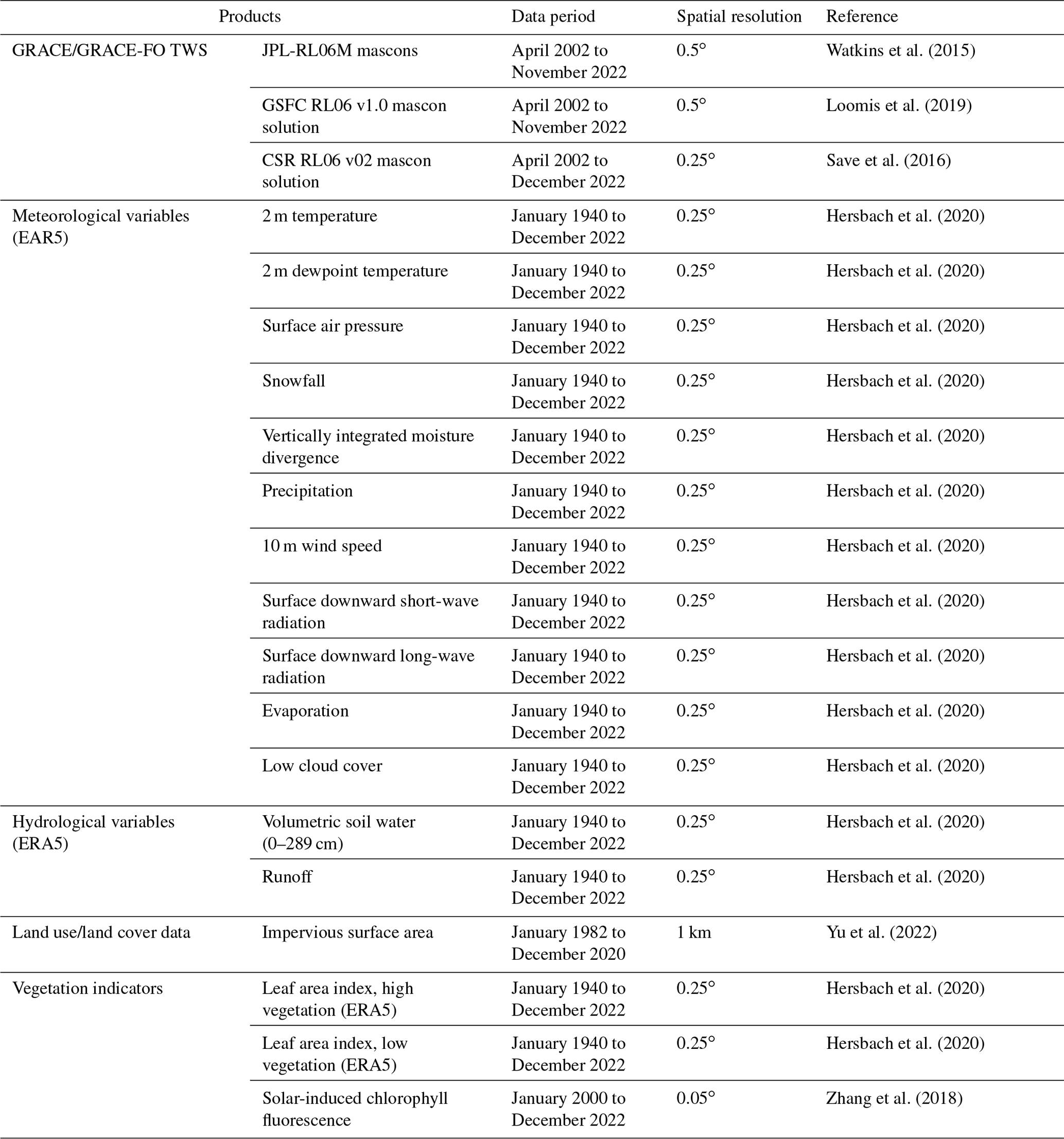
Three different GRACE/GRACE-FO solutions, which cover the monthly TWS series over the period 2002–2022 and are based on a mass concentration technique, are employed. This newly developed algorithm provides estimations of mass variations over small and predefined regions, which are briefly referred to as mascons (Watkins et al., 2015). The mascon solutions are usually better than the spherical harmonics-based products, for example, it reduces leakage due to increased signal amplitude and it requires fewer or no postprocessing procedures (Scanlon et al., 2016). We use the latest mascon-based products from three international centers: the Jet Propulsion Laboratory (JPL) of California Institute of Technology, the Center for Space Research (CSR) at the University of Texas at Austin, and the Goddard Space Flight Center (GSFC) of NASA. The TWS products based on the three mascon solutions are divergent, because they are produced by different processing methods and different models are employed for correcting the effect of glacial isostatic adjustment. The GRACE/GRACE-FO TWS estimates are employed to train our machine learning model to obtain the long-term reconstruction. The three mascon solutions have different spatial resolution due to divergent processing methods (Table 1). Although the GRACE/GRACE-FO datasets have some limitations, such as spatial and temporal coarseness, they are the best available training data even if their measurements can be further improved.
2.2 Inputs for the machine learning models
Numerous meteorological or hydrological variables have been identified as important elements in TWS reconstructions by previous works (e.g., Sun et al., 2020; Li et al., 2021). Here, we use four types of predictors to feed the machine learning model, including (1) 11 meteorological elements from the fifth generation European Centre for Medium-Range Weather Forecasts reanalysis (ERA5), (2) two hydrological variables from ERA5, (3) land use/land cover data, and (4) vegetation indicators, i.e., LAI and solar-induced fluorescence (SIF). The 11 meteorological variables consist of 2 m temperature (∘), near-surface specific humidity (kg kg−1) and relative humidity (%), snowfall (mm), vertically integrated moisture convergence (kg m−2 s−1), precipitation (mm), 10 m wind speed (m s−1), surface downward short-wave and long-wave radiation (W m−2), evaporation (mm), and cloud cover (%). These variables are selected due to their representation of water flux (e.g., precipitation and moisture convergence), energy flux (e.g., temperature, radiation and cloud cover), and other processes (i.e., wind speed) involving water–energy transport. Moisture convergence is represented by the negative value of vertically integrated moisture divergence in ERA5, and the cloud cover data refer to the proportion of a grid covered by clouds occurring in the lower levels of the troposphere.
The near-surface relative humidity (RH) and specific humidity (SH) are not currently available in the ERA5 monthly ensemble dataset, which can be estimated by using 2 m temperature (T2 m), dewpoint temperature (Tdew), and air pressure (pr). The Clausius–Clapeyron relationship describes the dependence of atmospheric saturation vapor pressure on air temperature as follows:
where T and esat indicate the near-surface air temperature (∘) and saturation vapor pressure (Pa), respectively; Lv and Rv refer to the latent heat of vaporization (2.5 × 10⁶ J kg−1) and vapor gas constant (461 J kg−1 K−1), respectively; and T0=273.15 K and es0=611 Pa are both integration constants.
The Tdew denotes the temperature above which the air moisture will be saturated under constant water vapor content and pressure; therefore, it can characterize the actual atmospheric water vapor availability. The RH can be calculated by substituting T2 m and Tdew into Eq. (1) as .
SH represents the mass contribution of water vapor to the total air mixture, which can be derived by pr and Tdew:
Hydrological variables, such as runoff and soil moisture, have been shown to be highly correlated with TWS (Sun et al., 2020; Yang et al., 2023), and therefore these two variables also served as predictors in the reconstruction model. For soil moisture, we use the average volumetric soil water of four layers weighted by the layer depth. Numerous studies have reported that land use/land cover change has substantial impacts on TWS, for example, changes in impervious surface area (ISA) due to urbanization play an essential role in driving TWS variability (Chen et al., 2018; Wang et al., 2020). To constrain the TWS by considering the effects of urbanization, we have extracted the ISA series from the latest FROM-GLC Plus product using Google Earth Engine. The pixel-based ISA is calculated from a multi-temporal (i.e., from daily to annual) and multi-resolution (i.e., ranging from sub-meter to 30 m) global land cover product (Yu et al., 2022). We use ISA to represent land cover changes to simplify the inputs of our machine learning model, which enables more efficient inference beyond the training period. Vegetation and TWS also have a feedback relationship due to water–energy exchange through photosynthesis and respiration as well as vegetation's regulation of soil moisture (Yin et al., 2023a, b; Liu et al., 2023). Therefore, we also use LAI from ERA5 and the recent satellite-based machine-learning-generated SIF dataset by Zhang et al. (2018) to train our machine learning models. (For detailed information about the inputs in our machine learning model, see Table 1.)
2.3 Independent evaluation datasets
The two most widely used global TWS reconstruction datasets (0.5∘ resolution) are used for comparison, i.e., the GRACE-REC dataset by Humphrey and Gudmundsson (2019) and the recent GRACE-like reconstructed TWS dataset (i.e., denoted as GRL-REC dataset hereafter) by Li et al. (2021). The GRACE-REC dataset is produced based on two GRACE/GRACE-FO solutions and three meteorological forcing products, and therefore releases six reconstructed datasets which includes 100 members within each data scheme. To facilitate the comparison, we average these six series to produce an ensemble average reconstructed TWS product, as it has already been shown that the blended product captures the GRACE-measured TWS dynamics well (Yin et al., 2023a). To evaluate the performance of our GTWS-MLrec reconstruction, we also try to close the ocean mass budget by using the global mean sea level (GMSL) from altimeter data (Nerem et al., 2018) and steric height estimates (GMSL_ster) based on measurements of Argo profiling floats (Levitus et al., 2012). In this study, we use total steric level (i.e., the sum of thermosteric and halosteric sea level) of the 0–700 m layer of the ocean. As the GMSL_ster dataset only provides seasonal series after 2005, we combine the seasonal GMSL_ster series and the running pentanal (i.e., 5 years) series prior to 2005. We also use TWS variations from the basin-scale water-balance dataset (BSWB) as an independent reference dataset. The BSWB dataset derived monthly variations in large-scale TWS for 341 large catchments (i.e., area >10 000 km2) worldwide by employing a hybrid atmospheric and terrestrial water budget technique (Hirschi and Seneviratne, 2017).
As the BSWB only provides TWS variation estimates during 1979–2015, we also try to evaluate the accuracy of TWS reconstructions by exploring their relationship with annual streamflow over a larger number of catchments. To achieve this goal, we gather daily river streamflow records from 1940 to the present at 22, 538 hydrological gauges from multiple sources. These records are sourced from a large combination of national and global data archives: (1) the Global Runoff Data Centre (GRDC); (2) the UK Centre for Ecology and Hydrology (UKCEH); (3) the Environment and Climate Change Canada through the Water Survey of Canada (ECCC); (4) the U.S. Geological Survey National Water Information System (USGS); (5) the Australian Bureau of Meteorology (ABM); (6) the Brazilian National Water Agency (ANA); (7) the Ministry of Water Resources of China (MWRC); (8) the watershed management agencies affiliated with the MWRC; (9) the National Hydrological Information Centre of China; (10) Guangdong Provincial Bureau of Beijing River Administration, China; and (11) Chaohu Lake Research Institute, China. First, we omit those stations with a changing measurement instrument or station datum to keep data consistency. Second, we exclude gauges with less than 20 valid years of data (with >90 % completeness for each year). Finally, we screen the catchments, excluding those with a catchment area larger than 10 000 km2. Using the daily streamflow records, we calculate the monthly average runoff depth by considering streamflow observations and catchment area, where only those months with >90 % daily data completeness are considered. For each year with 12 valid monthly values, we sum the values to derive a yearly runoff depth by considering catchment area. Overall, these filtering steps leave 10 168 catchments with complete 10-year annual streamflow, which cover diverse climatic patterns and underlying surface conditions across the globe.
2.4 Machine-learning-based TWS reconstruction method
The workflow of this reconstruction approach contains five modules, which are illustrated in Fig. 1. First, we employ five different machine learning models as candidates for TWS reconstruction. Second, eight input schemes are built for each machine learning model. Third, the random forest (RF) associated with a moving-windows approach is employed to determine the dominant variables in each input scheme for each machine learning model. Fourth, the best-performing machine learning model is selected in terms of the TWS simulation performance in the test period. Finally, the simulation performance of the eight input schemes is rated, and the eight schemes are blended to produce the long-term TWS series at each pixel.
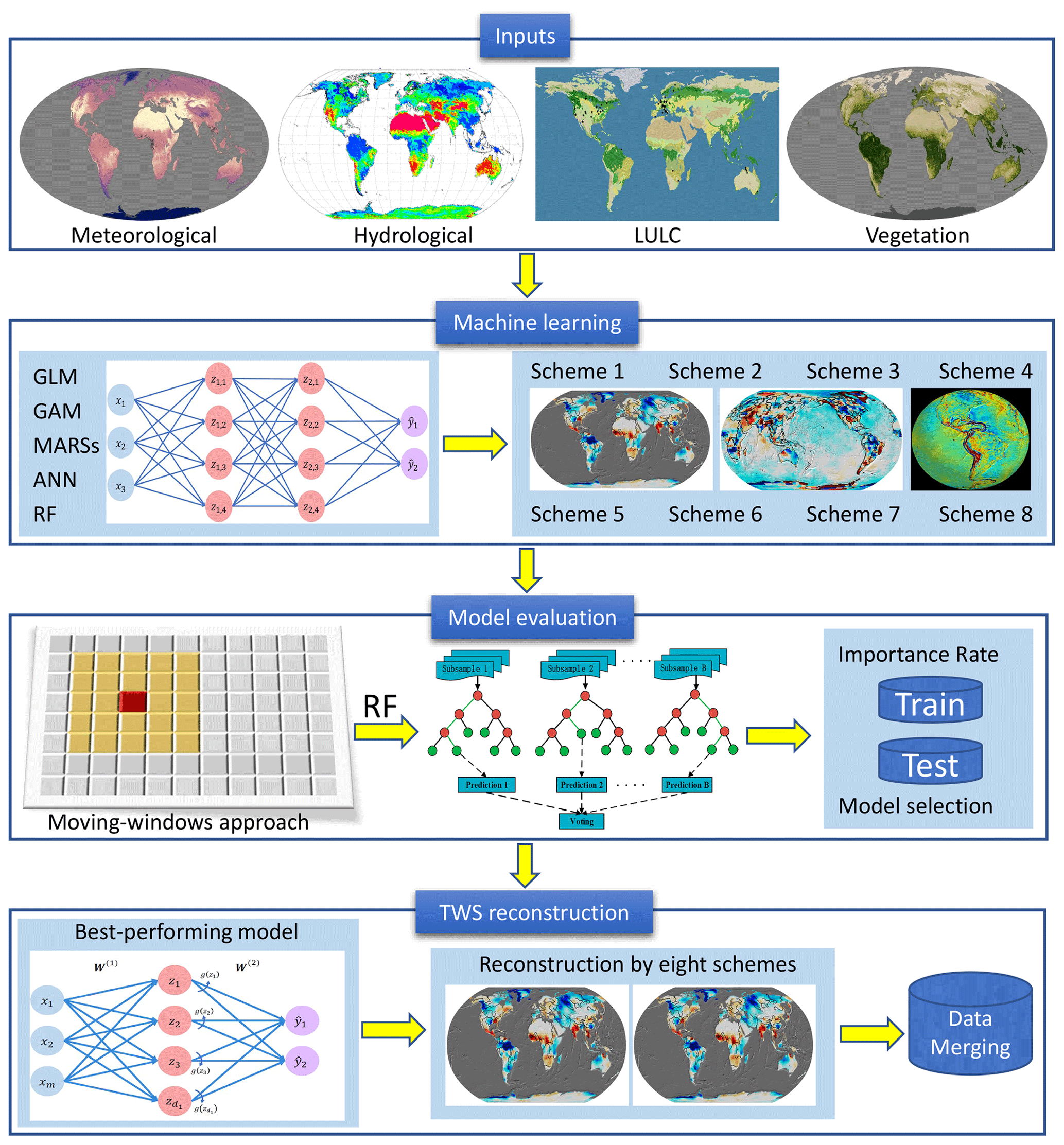
Figure 1Flowchart of the machine-learning-based TWS reconstruction approach.
The five data-driven (machine learning and statistical) models employed to establish the TWS reconstruction model are as follows: multivariate adaptive regression splines (MARSs), Gaussian linear regression model (GLM), artificial neural network (ANN), Gaussian generalized additive model (GAM), and an RF model. These five models employ the regression-based techniques to characterize the relationship between the predictors (i.e., dependent climate/vegetation variables) and the predictand (i.e., independent variables, TWS). The GLM is built within a parametric regression framework, while the other four models are based on a non-parametric regression algorithm, where the functional relationship has the feasibility of reliable adjustment to explore unusual or unexpected features (Shortridge et al., 2016; Singh et al., 2023). (For a more detailed illustration of these machine learning models, refer to the relevant references, e.g., Ghimire et al., 2021; Herath et al., 2021; Li et al., 2021.) For each machine learning model, eight different reconstruction schemes in terms of inputs are established: (1) scheme 1, containing all variables; (2) scheme 2, excluding LAI; (3) scheme 3, excluding SIF; (4) scheme 4, excluding LAI and SIF; (5) scheme 5, excluding land use and land cover (LULC); (6) scheme 6, excluding LULC and LAI; (7) scheme 7, excluding LULC and SIF; and (8) scheme 8, excluding LULC, LAI and SIF. We establish eight different data schemes because some variables might be missing during some periods, and by blending different data schemes we will be able to achieve a more complete long-term series. In all eight construction schemes, a time lag of 3 months is considered for the inputs, i.e., the data at the current time step and in the previous 1–3 months are both employed to feed the machine learning model. For example, in scheme 1, the input variables contain 64 time series of predictors as well as the GRACE/GRACE-FO TWS observations.
As TWS is governed by divergent physical mechanisms under different underlying surface conditions and climate patterns, the dominant variables for explaining the TWS may differ across different climatic regions (Yin et al., 2022a). Before establishing the TWS reconstruction model at each pixel, a moving-window nearest-neighbor approach is employed to select the most important variables for each pixel and its immediate neighbors. The moving-window nearest-neighbor approach is a good method to improve the robustness of machine learning methods, and it can also improve the training dataset for calibrating the machine learning model by assimilating richer information from nearby points. To balance data sample size and model complexity, we use a moving-window size of as 5 × 5 for each pixel. (We also tried a 3 × 3 moving-window size and found it was slightly less robust than the 5 × 5 scheme.) The RF is employed to select the most important 60 % of all candidate variables in each data scheme. The use of a moving window allows the model to be trained on a larger sample of data and to identify the most important candidate variables with greater consistency.
The eight data schemes for the five machine learning models are trained with GRACE/GRACE-FO data and multi-source inputs during 2002–2022 at each pixel, and their performance in simulating TWS is compared across the model–scheme combinations. Prior to building the machine learning models, all the data are normalized by using standard normalization techniques to standardize the features on a common numerical scale. To evaluate the performance of the reconstruction models, a cross-validation method is employed and the entire dataset is randomly split into training and testing parts. The training dataset (60 %) is employed to fit the models, while the remaining 40 % of data are used to test the model accuracy (40 %). The R package “randomForest” is adopted to implement the RF-based analysis (Breiman, 2001).
In the reconstruction procedure, we first select the best-performing machine learning model based on the evaluation index (see Sect. S1 in the Supplement) in scheme 8 during the test period, and then rate the simulation performance of the eight data schemes within the best-simulating machine learning model. We select scheme 8 for the best-simulating machine learning model, because this scheme contains the least volume of inputs and is more suitable for data extrapolation. After determining the best-performing model, we reconstruct the long-term TWS series by considering the scores of all the eight data schemes. In cases where variables might be missing for certain time periods, the best-performing scheme cannot be applied. To solve this issue, we make full use of the eight data schemes. For example, the best-performing scheme of the selected machine learning model is used to produce the TWS reconstructions, and then the second-best-performing scheme for the same model is used to fill any missing gaps of the former one. To improve the capacity of the machine learning models to extrapolate TWS series beyond the calibration period, we employ all the observations to train our model in the reconstruction process. However, we also evaluate the performance of extrapolation by splitting train and test periods in Sect. 3.3. By blending the different data schemes with consideration of their simulation performance, the TWS series for the long-term period (i.e., 1940–2022) is fully reconstructed. Using three different training GRACE/GRACE-FO datasets (i.e., JPL, CSR, and GSFC), we produce three different GTWS-MLrec datasets. As many studies focus on exploring climate-driven TWS variability, we also produce three detrended and de-seasonalized TWS reconstruction series. To achieve this goal, we first employ the seasonal-trend decomposition method based on Loess (Rojo et al., 2017) to partition the GRACE-measured series into linear, seasonal, and residual trends. The residual component from the GRACE-measured temporal series is then reconstructed separately by using their empirical relationships as related to the potential predictors (i.e., components after detrending and de-seasoning from the input variables). Therefore, we produce three full-component TWS datasets as well as three detrended and de-seasonalized TWS datasets across all global land areas for the period 1940–2022.
3.1 Six GTWS-MLrec datasets
The GTWS-MLrec provides monthly TWS anomalies in units of millimeters of water (mm) during 1940–2022, with a spatial resolution of 0.25∘ across global land areas (including Greenland and Antarctica). Using three different training GRACE/GRACE-FO mascon solutions (Table 1), we produce three different GTWS-MLrec datasets. We also provide de-seasonalized and detrended TWS anomalies, which are independently reconstructed by using the de-seasonalized and detrended GRACE/GRACE-FO dataset and inputs. It is informative to note that these de-seasonalized and detrended TWS reconstructions are not necessarily systematically consistent with the reconstructed TWS datasets after the de-seasonalizing and detrending processes, because they are reconstructed by using independent machine learning models. Therefore, we provide a total of six reconstructed GTWS-MLrec datasets trained by three GRACE/GRACE-FO solutions.
3.2 Global land mean TWS datasets
To provide data reference for a global-scale application, we also estimate a global average time series of the GTWS-MLrec TWS anomalies. The global mean TWS series is estimated by considering the area weight (i.e., the area of grid in different latitudes is considered), which includes all land areas with or without considering the Greenland and Antarctica (i.e., two schemes are available). These global average TWS datasets can provide rich information as references in constraining a global-scale water dynamic, which is particularly suited for quantifying a global land–ocean water budget. The global average TWS has a unit of millimeters of water. To convert millimeters to gigatons of water for mass budget applications, total land areas of 148 940 000 km2 and 132 773 914 km2 can be used for each scheme, respectively.
3.3 Performance of machine learning model in extrapolating TWS beyond the calibration period
Before using the machine learning models for the TWS reconstruction, we evaluate their extrapolation performance by randomly splitting the datasets into train and test periods during the GRACE/GRACE-FO era. Eight metrics are used (Sect. S1), including Pearson's correlation coefficient (PCC), Nash–Sutcliffe efficiency coefficient (NSE), Kling–Gupta efficiency coefficient (KGE), coefficient of determination (R2), root mean square error (RMSE, in millimeters), normalized root mean square error (nRMSE), mean absolute percentage error (MAPE), and percent bias (Pbias, in percent). Figure 2 presents the performance of the JPL-based reconstruction in data scheme 8 during the test period in comparison with the GRACE/GRACE-FO measurements. The PCC, NSE, KGE, and the R2 approach 0.9 in most areas of the globe for the test period, and the average nRMSE over the global land areas is about 0.1. The MAPE, RMSE, and Pbias also suggest a good performance. Comparing the five machine learning models, we find that the non-linear models (i.e., RF and ANN) show better performance than the linear models (i.e., GLM, GAM, and MARSs). The GAM, MARSs, and ANN also show a relatively reliable performance in extrapolating TWS anomalies, with the global average PCC of about 0.7, and the GLM shows the worst performance in most areas of the globe (Fig. S1 in the Supplement). We also compare the extrapolation performance for GSFC and CSR solutions and find similar conclusions, namely that the RF and ANN show better capacity in simulating TWS anomalies in most areas of the globe. Overall, we are confident that the best-simulating machine learning model allows us to reliably extrapolate TWS series beyond the calibration period.
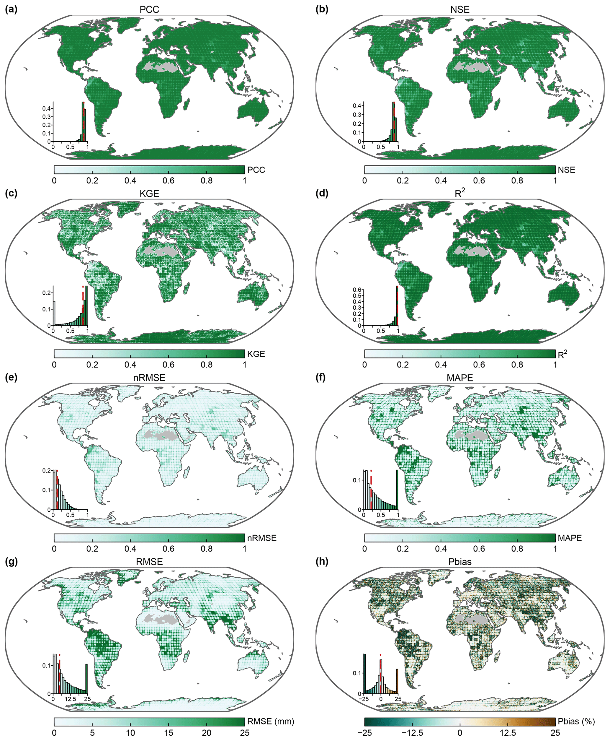
Figure 2Performance of random forest in simulating JPL TWS anomalies under scheme 8 during the test period: (a) PCC, (b) NSE, (c) KGE, (d) (R2), (e) nRMSE, (f) MAPE, (g) RMSE, and (h) Pbias. Insets in each panel show the histogram of these metrics, with the vertical red line showing the median value. Data-sparse areas without reconstruction are marked in gray.
4.1 Comparison with GRACE/GRACE-FO observations
The final reconstructed long-term GTWS-MLrec datasets under the best-performing model are compared with GRACE/GRACE-FO observations. Unlike the comparison in Sect. 3.3 focusing on the test period, this section evaluates the performance of GTWS-MLrec datasets in simulating the observations. The PCC, NSE, KGE, and R2 are larger than 0.9 in most land areas of the globe, and the nRMSE, MAPE, RMSE, and Pbias also suggest low biases in most land areas (Figs. 3, S2, and S3). We compare the values of these evaluation metrics with the scores achieved from previous reconstruction datasets (i.e., GRACE-REC and GRL-REC), which are also evaluated with respect to the corresponding training GRACE/GRACE-FO solutions (Figs. S4 and S5). Across all the metrics, GTWS-MLrec typically achieves better scores than the previous two datasets. GTWS-MLrec, in particular, shows substantially lower values of nRMSE, MAPE, RMSE, and Pbias than GRACE-REC and GRL-REC. It is informative to emphasize that unlike the GRACE-REC and GRL-REC datasets, which only reconstruct detrended and/or de-seasonalized TWS components, the three products of GTWS-MLrec provide the total components of TWS like GRACE/GRACE-FO observations. Therefore, it is not surprising that this reconstruction dataset shows such better performance when comparing with the observations.
The global yearly maps of reconstructed TWS fields are shown during the most recent strong El Niño years, i.e., 2015–2016. We find that GTWS-MLrec is able to capture the water storage anomalies due to the strong El Niño events. For example, eastern South America witnessed strong water deficits while most regions of South America suffered from severe flooding events during the onset period of El Niño in 2015 (Fig. S6). By the wakening period of El Niño events in 2016, western and northern South America suddenly switched from pluvial floods to water deficit conditions (Fig. S7). The El Niño–Southern Oscillation (ENSO) is one of the leading climate oscillations and often leads to extreme hydrological hazards over tropical regions (Fang et al., 2024); therefore, the anomalies in TWS over South America could be related to the strong El Niño events from the hydrological perspective (Ni et al., 2018; Li et al., 2021). From the GRACE/GRACE-FO observations and our reconstructions, we also find that the 2015–2016 El Niño brought strong pluvial floods in southern China and most areas of Australia, and brought droughts to India, the Middle East, central Europe, and western America. The yearly TWSA map of the previous two reconstruction datasets (i.e., GRACE-REC and GRL-REC) are also depicted. We find that these two previous datasets also captured the El Niño event, but the GRACE-REC dataset failed to capture the fluvial signal in some regions such as southern Australia. In addition, GTWS-MLrec can also capture water deficit or wetness conditions in other strong El Niño events such as in 1983 and 1998 (Fig. S8). Overall, all the above results suggest that our reconstructions reliably characterize the anomalies induced by strong El Niño events, which is in line with the GRACE/GRACE-FO measurements.
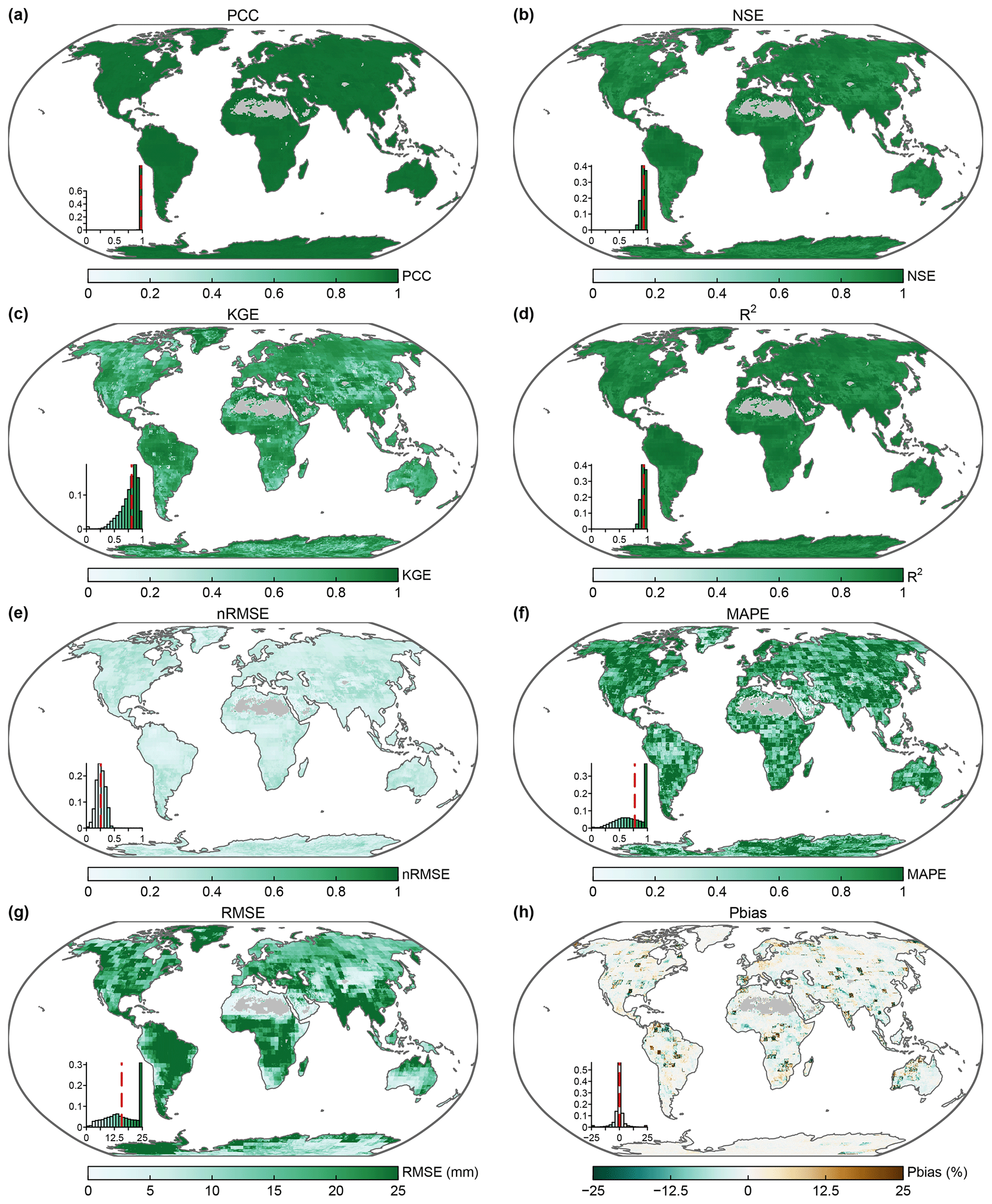
Figure 3Comparison of our JPL-based GTWS-MLrec reconstructions with the GRACE/GRACE-FO observations: (a) PCC, (b) NSE, (c) KGE, (d) (R2), (e) nRMSE, (f) MAPE, (g) RMSE, and (h) Pbias. Insets in each panel show the histograms of that evaluation metric, with the vertical red line showing the median value. Data-sparse areas without reconstruction are marked in gray.
To evaluate the performance of GTWS-MLrec in capturing the global average TWS anomalies, we also present the long-term monthly TWS anomalies over global land areas with and without Greenland and Antarctica (Fig. 4). During the GRACE era (2002–2022), the reconstructed TWS products do capture the inter-annual and seasonal cycle of GRACE/GRACE-FO observations well. Our three GTWS-MLrec products show similar long-term trends, which all indicate a decreasing change in the global average TWS anomalies. By comparing GTWS-MLrec with the GRACE-REC and GRL-REC datasets, we find that the reconstruction captures the inter-annual pattern of GRACE-REC well, while the GRL-REC dataset shows a slight overestimation phenomenon relative to our reconstruction and the GRACE-REC. Overall, the evaluations between GTWS-MLrec and GRACE/GRACE-FO observations indicate that our products achieve a good simulation performance at both grid and global scale.
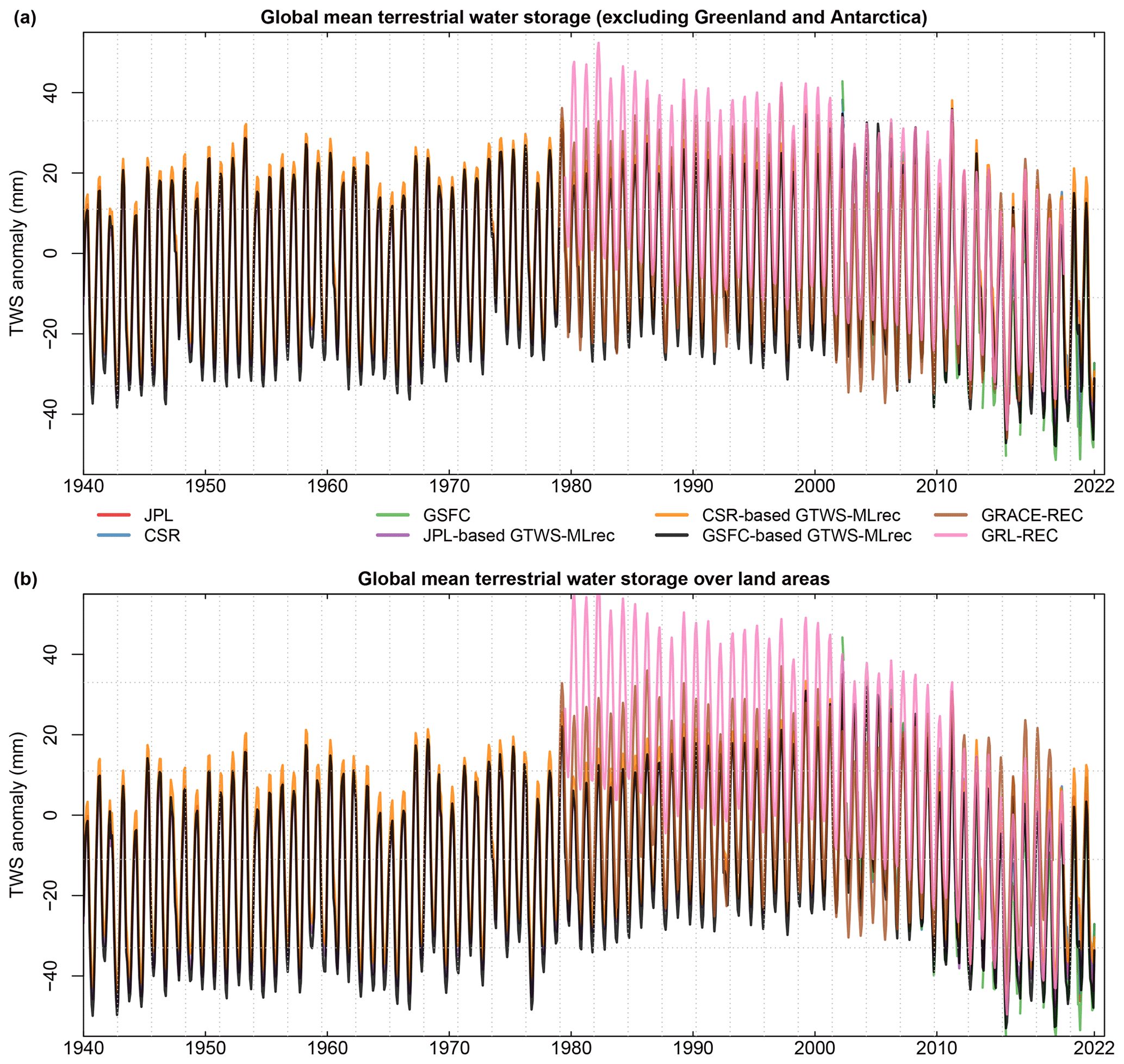
Figure 4Global mean monthly terrestrial water storage anomaly derived by eight different datasets (including GRACE/GRACE-FO observations). Panel (a) shows the global average TWS anomaly weighted by land area excluding Greenland and Antarctica. Panel (b) shows global average TWS anomaly over land areas.
4.2 Performance evaluation based on ocean–land water budget
Although the atmosphere holds moisture and thus can contribute to ocean mass changes by precipitation/evapotranspiration alternations, variations in ocean mass usually coincide with a comparable and opposite change of land water storage at a relatively long temporal scale (Chambers et al., 2017; Seo et al., 2023). Therefore, the sea level-based land–ocean mass budget provides an independent way to evaluate estimates of global average TWS variability. Here we assess the capacity of observed and reconstructed TWS products (GRACE/GRACE-FO, GTWS-MLrec, GRACE-REC, and GRL-REC) to constrain the sea level budget. The GMSL is employed to present ocean mass changes after subtracting the steric thermosteric and halosteric sea level. From the sea level budget-based analysis, we derive the time series of de-seasonalized and detrended changes in ocean mass, which we compare with converted global average TWS estimates with consideration of land–ocean area (estimated after removing the trend and seasonal signal from the primary datasets). To ensure a consistent comparison among all candidate products, Greenland and Antarctica are excluded when calculating the global average land TWS series. The comparison results show that, although all candidate datasets are well correlated with the ocean-mass-based water budget, GTWS-MLrec and the GRL-REC product exhibit the strongest correlation with GMSL, with PCC values of >0.7 during 2006–2020 (Fig. 5). Surprisingly, the reconstruction datasets also yield better results than the original GRACE/GRACE-FO datasets. This phenomenon has also been reported in previous studies (Humphrey and Gudmundsson, 2019), probably because the global average GRACE/GRACE-FO TWS is more susceptible to non-compensating continental-scale errors (e.g., caused by biases from residual longitudinal stripes) compared with the data-driven reconstructions, which achieve smoother global average series. To evaluate our independent detrended and de-seasonalized GTWS-MLrec datasets, we also compare their converted TWS series with the GMSL. This converted dataset is different from directly excluding the trend and seasonal cycles from the full-component reconstruction datasets. The three detrended and depersonalized GTWS-MLrec datasets also show a good agreement with the global ocean mass changes, with a PCC ranging from 0.61 to 0.66 (Fig. 6). All the results suggest that both of our reconstruction types are able to constrain the ocean–land water budget.
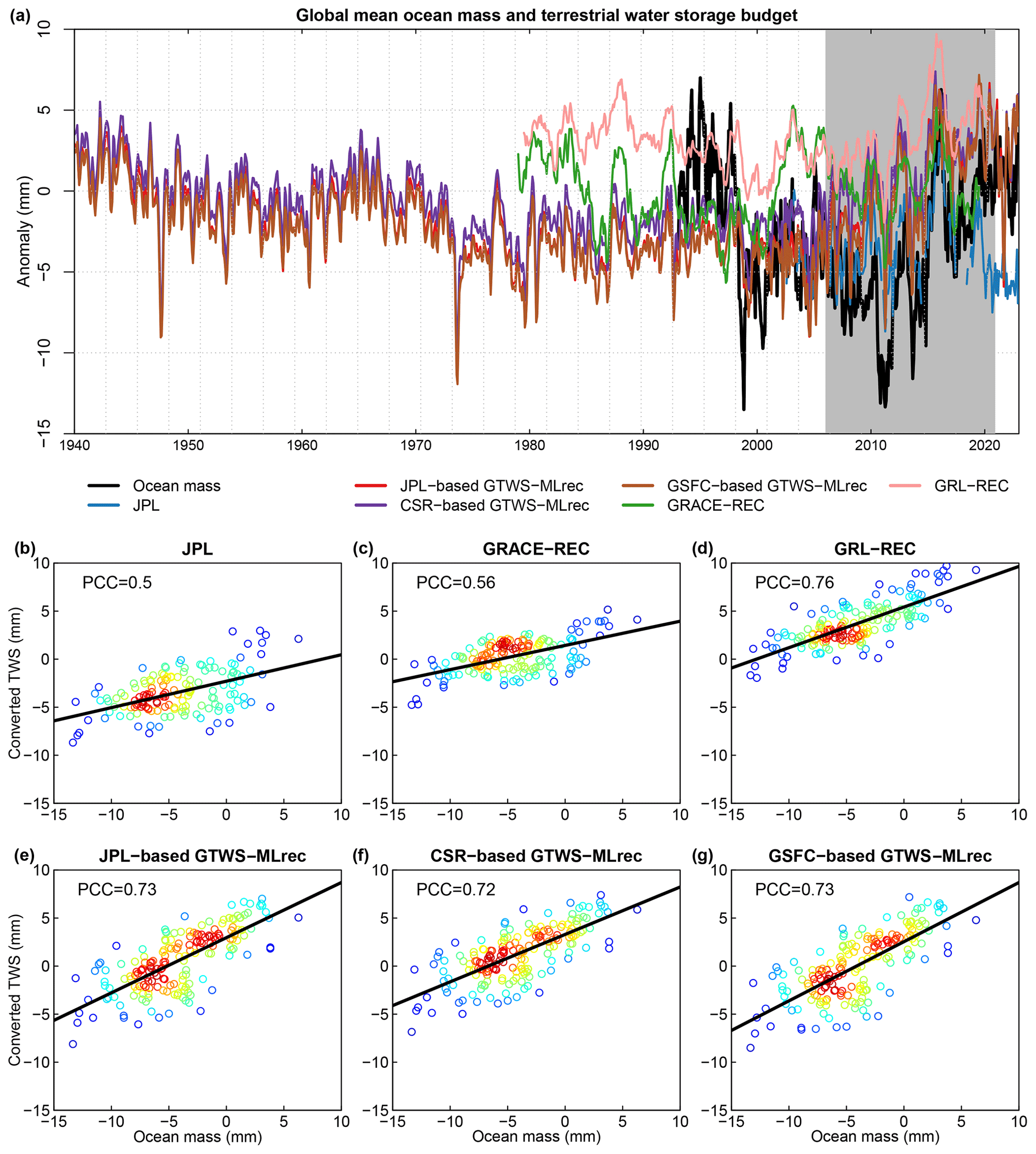
Figure 5Comparison of the global average TWS variations (converted to equivalent sea level, in millimeters) against ocean mass changes derived from the sea level budget. Panel (a) shows the temporal dynamics of the global average sea level and TWS. Panels (b–g) show the regression plots of the sea level and converted TWS. The redder colors indicate higher, and the bluer colors lower, density of points. The black line denotes the linear regression. The converted TWS is estimated after extracting the trend and seasonal signals from the negative values of primary datasets by considering the land–ocean area ratio.
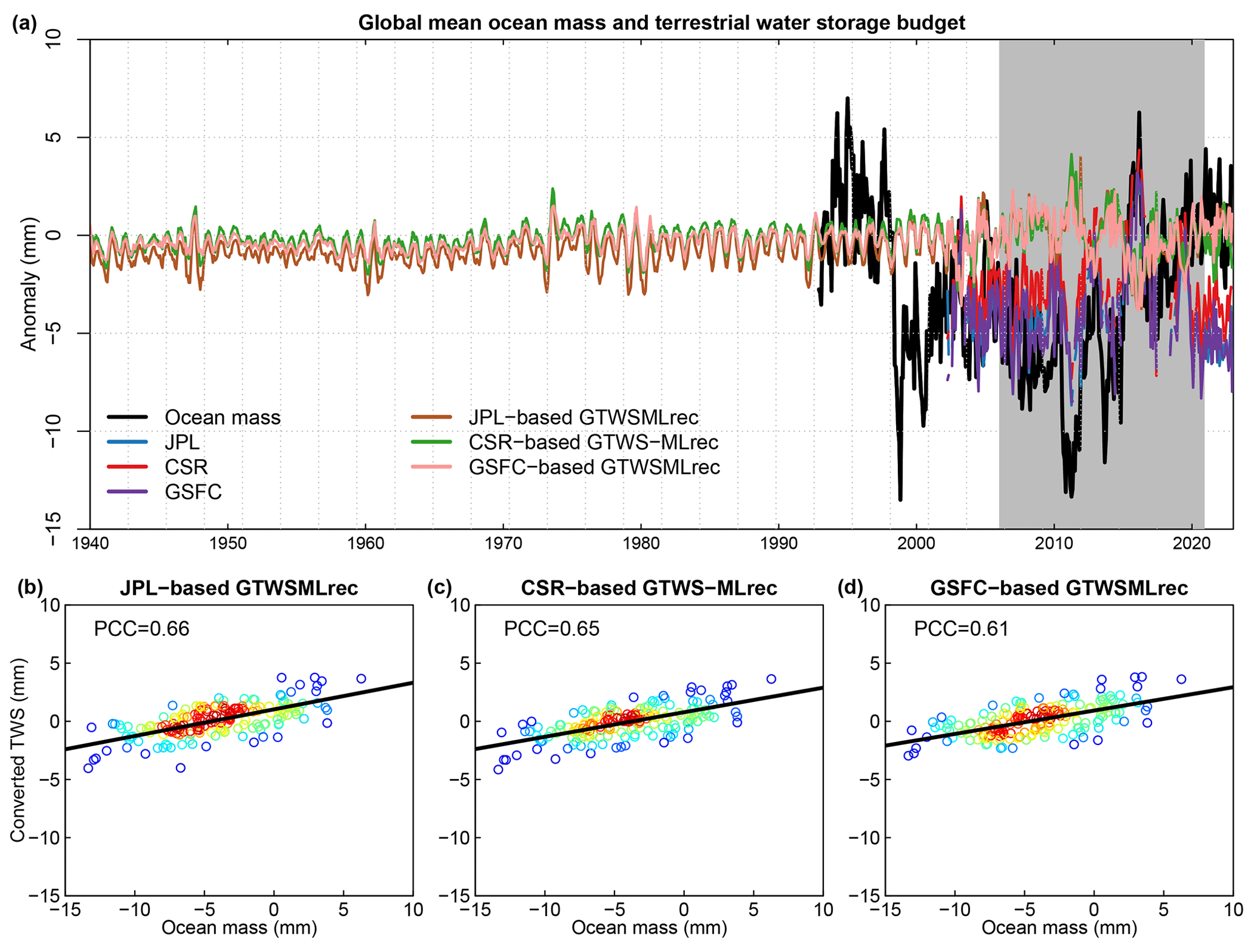
Figure 6Global land–ocean mass budget based on our reconstructed detrended and de-seasonalized GTWS-MLrec datasets. Panel (a) shows temporal dynamics of global average sea level and TWS. Panels (b–d) show regression plots of sea level and converted TWS. The redder colors indicate higher, and the bluer colors lower, density of points. The black line denotes the linear regression. The converted TWS is estimated as the negative values of primary detrended and de-seasonalized reconstruction datasets by considering the land–ocean area ratio.
4.3 Performance evaluation based on water balance over large river basins
It is challenging to directly evaluate the performance of the TWS reconstructions prior to 2002 due to lack of GRACE/GRACE-FO observations. However, as TWS is a key element linking the atmospheric and terrestrial water balance budget, it is possible to independently evaluate the reconstructions by combining land and atmospheric moisture fluxes (Oki et al., 1995; Yin et al., 2022a). Hirschi and Seneviratne (2017) presented the BSWB dataset, which assimilated in situ streamflow observations and reanalysis-based moisture convergence in the atmosphere, and provided monthly variations in TWS during 1979–2015 in 341 moderately large river basins (>100 000 km2) covering a variety of climate conditions. To provide a more comprehensive evaluation of our reconstructions, we extracted the variations in TWS from our reconstructions over the same basins as the BSWB dataset. As a caveat, we note that the BSWB is derived from the predecessor of the ERA5 dataset (i.e., ERA-Interim), which is not entirely consistent with the main drivers of GTWS-MLrec products. Overall, both the GRACE/GRACE-FO and the reconstructed datasets do agree with the BSWB-based TWS variations well (Fig. 7a–h). For the JPL-, CSR-, and GSFC-based mascons, these products show a PCC with BSWB ranging from 0.4 to 0.7 over most basins, and the global average PCC is about 0.58. The larger catchments typically show higher PCC than the smaller catchments, which can be explained by the fact that the basin-averaged TWS series of larger catchments have been smoothed by using more gridded data. For GTWS-MLrec, the three reconstructed datasets show a relatively similar pattern of PCC over the moderately large global river basins, further verifying the robust performance of our reconstructions.
We also compare the BSWB-based TWS variations with the GRACE-REC and GRL-REC products, and find a slightly higher PCC of GRACE-REC and GRL-REC than GTWS-MLrec reconstructions. This phenomenon might be due to two reasons. First, our GTWS-MLrec is reconstructed by assimilating the latest ERA5 dataset, which has substantial updates relative to ERA-Interim (i.e., inputs of BSWB). Second, the BSWB and two previous reconstruction datasets both mainly focused on climate-driven changes in TWS but neglected underlying surface condition changes such as vegetation greening due to increases in LAI and human-made infrastructures such as reservoirs. GTWS-MLrec not only assimilates climate variables but also captures changes in underlying surface conditions; therefore, these results may cause biases when comparing with the BSWB dataset. For example, the basins in China's Yangtze River usually show a higher PCC of previous reconstruction datasets than GTWS-MLrec. The Yangtze River has experienced rapid urbanization and reservoir constructions in recent decades (Gu et al., 2019), where the BSWB and previous reconstruction datasets have a similar TWS pattern. We also compare the TWS variations of uncorrected and drift-corrected series from the BSWB with GTWS-MLrec, and find that the drift-corrected version of BSWB shows a slightly higher PCC with GTWS-MLrec (Fig. 7i–j), suggesting that the temporal smoothing improves TWS estimates by constraining the basin-scale water budget. Overall, our GTWS-MLrec achieves a relatively good agreement with the BSWB-based TWS variations in most large basins over most large basins of the globe.
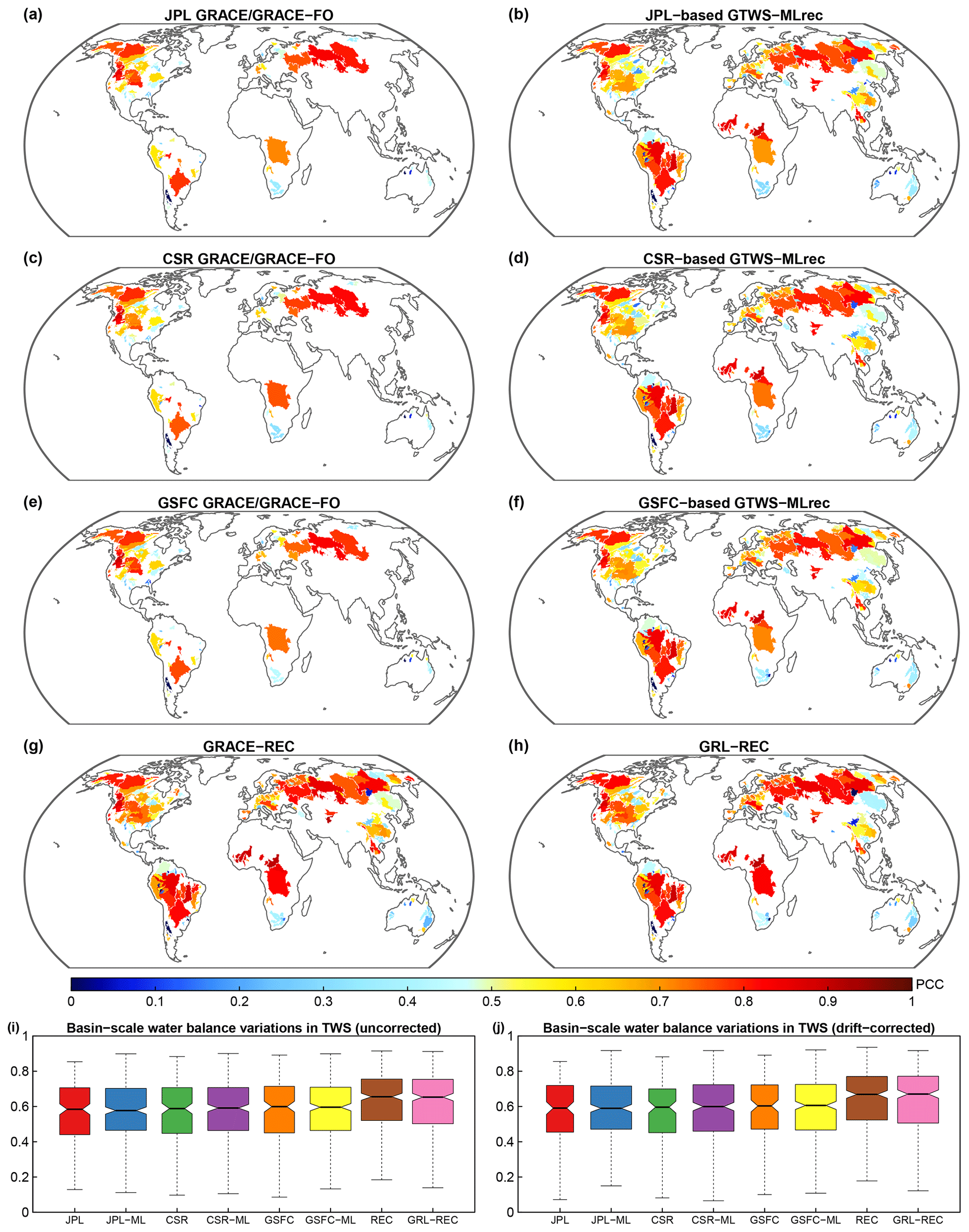
Figure 7Comparison between variations in TWS derived from the atmospheric basin-scale water balance (BSWB) dataset, GRACE/GRACE-FO measurements, and reconstructions. Panels (a–h) show the PCC of drift-corrected BSWB-based TWS and observation/reconstruction datasets. Panels (i–j) show boxplots of global PCC between BSCB and different TWS datasets for uncorrected (i) and drift-corrected (j) BSWB datasets. In panels (i) and (j), the JPL (or CSR, GSFC) denotes GRACE/GRACE-FO observations, and the JPL-ML (or CSR-ML, GSFC-ML) denotes GTWS-MLrec reconstructions. The REC denotes GRACE-REC.
4.4 Comparison with annual streamflow measurements
As the BSWB dataset only provides TWS variations over large basins after 1979, we obtained streamflow data extending to 1940 from multiple sources, including the GRDC, USGS, and MWRC. After strict data quality control and screening of the data records from 22 538 stations, we retained 10 168 hydrological stations in basins smaller than 100 000 km2 with at least 10-year complete monthly streamflow series (see Sect. 2.3). River streamflow and TWS of course represent different hydrological elements with divergent units; however, their temporal dynamics at a longer timescale (i.e., yearly) might be correlated because runoff is an important water flux component in the total water storage (Rodell and Li, 2023; Yin et al., 2023b). In addition, a drier (or wetter) river streamflow state at an annual scale is usually related to anomalies in large-scale atmospheric circulation, which is also represented by a similar signal indicated by annual TWS variations (Kang et al., 2023; Yin et al., 2023a). To provide a better comparison with the basin-scale streamflow, the TWS from different reconstruction datasets were aggregated at the watershed scale to obtain the catchment mean annual series in each basin using the Thiessen polygon method. The mismatch in resolution between large-scale mass changes and local basin streamflow dynamics can be partly alleviated by the spatial coherence of annual anomalies in weather/climate patterns. First, we compare the basin-scale TWS against streamflow during 1979–2022 and find that GTWS-MLrec agrees well with the observational streamflow dynamics at a yearly scale (Fig. 8). The JPL- and GSFC-based GTWS-MLrec datasets both show a global average PCC of 0.58, whereas the CSR-based reconstruction achieves a higher global average PCC of 0.60. The slightly better performance of the CSR-based GTWS-MLrec product may be due to the fact that the primary CSR mascon solution has a finer spatial resolution than the other two products. The previous GRACE-REC and GRL-REC reconstruction datasets show poorer performance than GTWS-MLrec products in terms of the PCC. The GRACE-REC and GRL-REC datasets show a global average PCC of 0.56 and 0.47, respectively. These results suggest that GTWS-MLrec achieves the best performance relative to streamflow in terms of reproducing past water cycle variability. In addition, the streamflow and TWS from our three reconstructions are compared during 1940–1980 (Fig. 9). Our GTWS-MLrec products show a global average PCC of 0.55–0.57, and the CSR-based dataset still shows the best performance, suggesting a good agreement with the temporal streamflow dynamics.
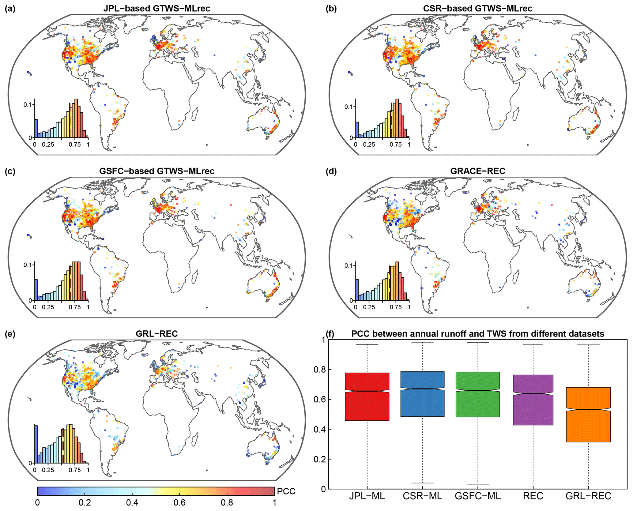
Figure 8Correlation of annual streamflow and aggregated basin-scale TWS from the different reconstruction datasets during 1979–2022. Panels (a–e) show global distribution of PCC for the different datasets, and (f) shows a boxplot of the PCC for all stations globally. The REC denotes GRACE-REC. Insets in (a–e) show the histogram of these metrics and the vertical red line shows the median value.
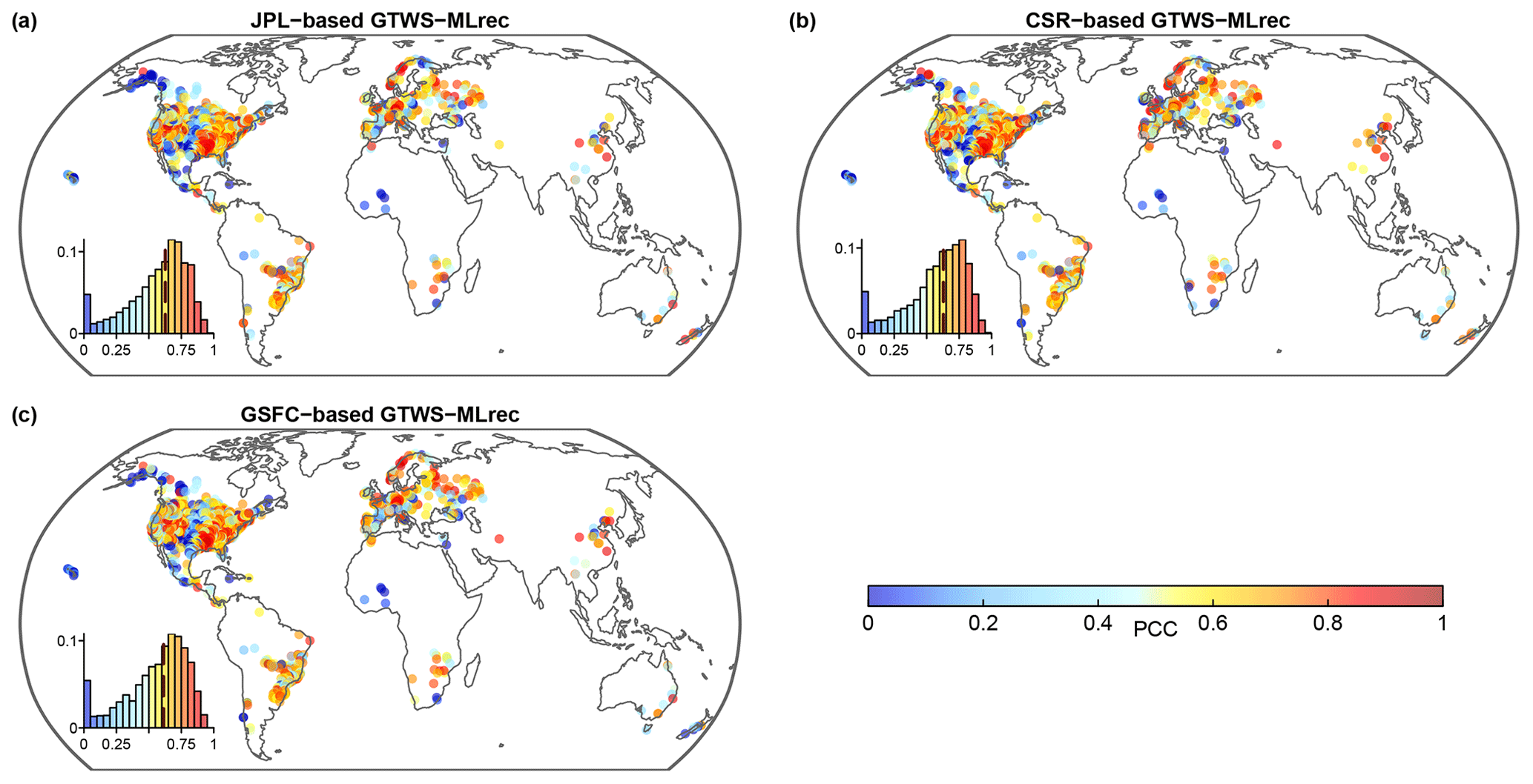
Figure 9Correlation of annual streamflow and aggregated basin-scale TWS from different reconstruction datasets during 1940–1980. Panel (a) shows JPL-based GTWS-MLrec, (b) CSR-based GTWS-MLrec, and (c) GSFC-based GTWS-MLrec. Insets in each panel show the histogram of these metrics and the vertical red line shows the median value.
The GTWS-MLrec dataset is archived on Zenedo at the link: https://doi.org/10.5281/zenodo.10040927 (Yin, 2023). It is distributed with a CC-BY license. The uploaded data provided are (a) JPL-based GTWS-MLrec TWS series, (b) CSR-based GTWS-MLrec TWS series, (c) GSFC-based GTWS-MLrec TWS series, (d) JPL-based GTWS-MLrec TWS constructions after removing trend and seasonal signals, (e) CSR-based GTWS-MLrec TWS series after removing trend and seasonal signals, (f) GSFC-based GTWS-MLrec TWS series after removing trend and seasonal signals, (g) global average TWS series over land areas, and (h) global average TWS series over land areas after excluding Greenland and Antarctica.
TWS – which encompasses all water storage or fluxes on the land, such as groundwater, soil moisture, snow/ice cover, and surface water – is a key element affecting the hydrological cycle at both global and regional scales. TWS also plays an essential role in the global water and energy budget balance, which is highly correlated with underlying surface conditions (e.g., vegetation) and climate fluctuations (e.g., El Niño events). Thus, to improve our understanding of changes in the hydrological cycle under climate change, a long-term TWS dataset is urgently needed. However, direct remote sensing-based observations of TWS from the GRACE/GRACE-FO only go back to 2002. Therefore, recent works have retrospectively reconstructed TWS at global or regional scales (e.g., Humphrey and Gudmundsson 2019; Sun et al., 2020; Li et al., 2020, 2021). Despite being useful for various purposes, these studies have been usually constrained by the short time period (e.g., starting from 1979) or coarse spatial resolution (≥0.5∘). Furthermore, previous studies have often focused primarily on climate-driven changes in TWS and have not fully assimilated information about vegetation conditions such as LAI. GTWS-MLrec, the new TWS product presented here, provides a monthly TWS dataset from 1940 to the present at 0.25∘ and is reconstructed by assimilating a large number of meteorological, hydrological, human-relevant, and vegetation variables. By comparing GTWS-MLrec with GRACE/GRACE-FO observations, we find that GTWS-MLrec usually achieves a higher correlation coefficient and lower biases than previous reconstruction datasets. We also evaluate the performance of different reconstruction datasets by using the land–ocean mass budget, basin-scale water balance, and temporal streamflow dynamics, as well as their ability to capture El Niño events. These independent evaluations all suggest that our GTWS-MLrec achieves better performance than previous datasets under most conditions.
We envision that GTWS-MLrec, with its comprehensive and extensive attributes, could provide rich information as references across a broad range of geoscience-relevant applications. First, the long-term TWS series can provide rich information for understanding changes in the global and regional hydrological cycle under climate change. For example, the TWS-based drought index has shown great potential for monitoring and assessing large-scale droughts in numerous regions of the globe (Long et al., 2014; Yin et al., 2022a). Second, the TWS anomalies of GTWS-MLrec could be used as an independent benchmark to evaluate the performance of a set of hydrological/climate models. Numerous studies have compared the TWS produced by GRACE/GRACE-FO and hydrological models, and have found that many physical models tend to simulate an earlier peak of TWS in seasonal cycle, which may be related to an underestimation of the overall water storage capacity (Schellekens et al., 2017; Long et al., 2017). However, these comparisons were conducted over a short time period, whereas GTWS-MLrec will be helpful to achieve a more robust long-term assessment. Third, GTWS-MLrec will provide more useful information for understanding terrestrial carbon–climate feedbacks. As TWS reflects the water condition needed for vegetation growth, TWS variability is tightly coupled to the atmospheric CO2 growth rate (Liu et al., 2023). Therefore, our GTWS-MLrec could contribute to understanding the possible shifts in terrestrial climate–carbon coupling under climate change. Finally, GTWS-MLrec can also improve the understanding of the dynamic relationship between climate change and human activities, such as groundwater depletion (Long et al., 2020; Seo et al., 2023), irrigation (Lv et al., 2019), urbanization (Huang et al., 2023), compound hazards (Yin et al., 2022b), and reservoir operation (Shah et al., 2019).
Although GTWS-MLrec presents substantial improvements over previous TWS reconstructions and holds potential for a broad range of geoscience applications, a few caveats should be acknowledged. The main inputs for feeding the machine learning model are sourced from the ERA5 dataset, which provides hourly and monthly climatic variables at 0.25∘ spatial resolution. Many basin-scale hydrological studies may need a TWS dataset at a finer spatial resolution, where GTWS-MLrec may be too coarse to constrain the water budget balance. The ERA5-Land dataset is available at 0.1∘resolution but is not considered in this study because it lacks some key variables such as cloud cover and moisture divergence. The estimation accuracy of the TWS reconstruction relies on the quality of the ERA5 datasets, and next generations/versions of the TWS data could potentially be improved as ERA5 itself improves over time. We have evaluated the relationship between our reconstructed TWS and streamflow measurements at 10 168 gauges in terms of PCC. TWS and streamflow might have a non-linear relationship due to their different generating mechanisms. However, it is difficult to quantify their physical non-linear relationship due to observational data limitations. Previous studies also evaluated the performance of TWS reconstructions by exploring their linear relationship with streamflow (e.g., Humphrey and Gudmundsson, 2019; Li et al., 2021, 2022). In future works, a more complicated non-linear relationship between TWS and streamflow might further evaluate the performance of TWS reconstructions. Although we have tried to assimilate information of underlying surface conditions and vegetation states, the series of SIF and ISA cannot be extended to 1940 because they are constrained by the availability of historical satellite records. To address this issue, we have designed eight different data schemes in the machine learning models, and the long-term LAI series can also provide information about vegetation. The human-made hydraulic infrastructures, such as reservoirs, may play an important role in regulating TWS, but these effects have not been fully considered in the GTWS-MLrec. Future work may seek to incorporate more predictors in the long-term TWS reconstruction and to provide more systematic independent evaluations.
The supplement related to this article is available online at: https://doi.org/10.5194/essd-15-5597-2023-supplement.
JY conceived the study, performed the analyses, and wrote the manuscript. LJS, PL, FL, YP, and PG provided critical input and assisted in interpretation of the results. AK and LY contributed to data analysis by Google Earth Engine. All the co-authors reviewed and edited the manuscript.
The contact author has declared that none of the authors has any competing interests.
Publisher's note: Copernicus Publications remains neutral with regard to jurisdictional claims made in the text, published maps, institutional affiliations, or any other geographical representation in this paper. While Copernicus Publications makes every effort to include appropriate place names, the final responsibility lies with the authors.
The authors would like to thank the editors and anonymous reviewers for valuable comments and suggestions to improve this dataset.
Jiabo Yin is supported by the National Natural Science Foundation of China (grant nos. 52009091, 52242904, and 52261145744) and the Fundamental Research Funds for the Central Universities (no. 2042022kf1221). Louise J. Slater is supported by UK Research and Innovation (grant nos. MR/V022008/1 and NE/S015728/1). The numerical calculations in this paper were performed on the supercomputing system in the Supercomputing Centre of Wuhan University.
This paper was edited by Sander Veraverbeke and reviewed by two anonymous referees.
Ahmed, M., Sultan, M., Elbayoumi, T., and Tissot, P.: Forecasting GRACE Data over the African Watersheds Using Artificial Neural Networks, Remote Sens., 11, 1769, https://doi.org/10.3390/rs11151769, 2019.
Breiman, L.: Random Forests, Machine Learning, 45, 5–32, https://doi.org/10.1023/A:1010933404324, 2001.
Chambers, D. P., Cazenave, A., Champollion, N., Dieng, H., Llovel, W., Forsberg, R., von Schuckmann, K., and Wada, Y.: Evaluation of the Global Mean Sea Level Budget Between 1993 and 2014, in: Integrative Study of the Mean Sea Level and Its Components, edited by: Cazenave, A., Champollion, N., Paul, F., and Benveniste, J., Springer International Publishing, Cham, 315–333, https://doi.org/10.1007/978-3-319-56490-6_14, 2017.
Chen, Z., Jiang, W., Wang, W., Deng, Y., He, B., and Jia, K.: The Impact of Precipitation Deficit and Urbanization on Variations in Water Storage in the Beijing-Tianjin-Hebei Urban Agglomeration, Remote Sens., 10, 4, https://doi.org/10.3390/rs10010004, 2018.
Fang, L., Yin, J., Wang, Y., et al.: Machine learning and copula-based analysis of past changes in global droughts and socioeconomic exposures, J. Hydrol., 628, 130536, https://doi.org/10.1016/j.jhydrol.2023.130536, 2024.
Felfelani, F. Y., Wada, Y., Longuevergne, L., and Pokhrel, Y. N.: Natural and human-induced terrestrial water storage change: A global analysis using hydrological models and GRACE, J. Hydrol., 553, 105–118, https://doi.org/10.1016/j.jhydrol.2017.07.048, 2017.
Ghimire, S., Yaseen, Z. M., Farooque, A. A., Deo, R. C., Zhang, J., and Tao, X.: Streamflow prediction using an integrated methodology based on convolutional neural network and long short-term memory networks, Sci. Rep., 11, 17497, https://doi.org/10.1038/s41598-021-96751-4, 2021.
Gu, L., Yin, J., Gentine, P., Wang, H.-M., Slater, L. J., Sullivan, S. C., Chen, J., Zscheischler, J., and Guo, S.: Large anomalies in future extreme precipitation sensitivity driven by atmospheric dynamics, Nat. Commun., 14, 3197, https://doi.org/10.1038/s41467-023-39039-7, 2023.
Gu, X., Zhang, Q., Singh, V. P., Song, C., Sun, P., and Li, J.: Potential contributions of climate change and urbanization to precipitation trends across China at national, regional and local scales, Int. J. Climatol., 39, 2998–3012, https://doi.org/10.1002/joc.5997, 2019.
Herath, H. M. V. V., Chadalawada, J., and Babovic, V.: Hydrologically informed machine learning for rainfall–runoff modelling: towards distributed modelling, Hydrol. Earth Syst. Sci., 25, 4373–4401, https://doi.org/10.5194/hess-25-4373-2021, 2021.
Hersbach, H., Bell, B., Berrisford, P., et al.: The ERA5 global reanalysis, Q. J. Roy. Meteor. Soc., 146, 1999–2049, https://doi.org/10.1002/qj.3803, 2020.
Hirschi, M. and Seneviratne, S. I.: Basin-scale water-balance dataset (BSWB): an update, Earth Syst. Sci. Data, 9, 251–258, https://doi.org/10.5194/essd-9-251-2017, 2017.
Huang, X., Ding, K., Liu, J., Wang, Z., Tang, R., Xue, L., Wang, H., Zhang, Q., Tan, Z.-M., Fu, C., Davis, S. J., Andreae, M. O., and Ding, A.: Smoke-weather interaction affects extreme wildfires in diverse coastal regions, Science, 379, 457–461, https://doi.org/10.1126/science.add9843, 2023.
Humphrey, V. and Gudmundsson, L.: GRACE-REC: a reconstruction of climate-driven water storage changes over the last century, Earth Syst. Sci. Data, 11, 1153–1170, https://doi.org/10.5194/essd-11-1153-2019, 2019.
Humphrey, V., Gudmundsson, L., and Seneviratne, S. I.: A global reconstruction of climate-driven subdecadal water storage variability, Geophys. Res. Lett., 44, 2300–2309, https://doi.org/10.1002/2017GL072564, 2017.
Jacob, T., Wahr, J., Pfeffer, W. T., and Swenson, S.: Recent contributions of glaciers and ice caps to sea level rise, Nature, 482, 514–518, https://doi.org/10.1038/nature10847, 2012.
Kang, S., Yin, J., Gu, L., Yang, Y., Liu, D., and Slater, L.: Observation-constrained projection of flood risks and socioeconomic exposure in China, Earth's Future, 11, e2022EF003308, https://doi.org/10.1029/2022EF003308, 2023.
Kim, J.-S., Seo, K.-W., Jeon, T., Chen, J., and Wilson, C. R.: Missing Hydrological Contribution to Sea Level Rise, Geophys. Res. Lett., 46, 12049–12055, https://doi.org/10.1029/2019GL085470, 2019.
Kusche, J., Eicker, A., Forootan, E., Springer, A., and Longuevergne, L.: Mapping probabilities of extreme continental water storage changes from space gravimetry, Geophys. Res. Lett., 43, 8026–8034, https://doi.org/10.1002/2016GL069538, 2016.
Lettenmaier, D. P. and Famiglietti, J. S.: Water from on high, Nature, 444, 562–563, https://doi.org/10.1038/444562a, 2006.
Levitus, S., Antonov, J. I., Boyer, T. P., Baranova, O. K., Garcia, H. E., Locarnini, R. A., Mishonov, A. V., Reagan, J. R., Seidov, D., Yarosh, E. S., and Zweng, M. M.: World ocean heat content and thermosteric sea level change (0–2000 m), 1955–2010, Geophys. Res. Lett., 39, L10603, https://doi.org/10.1029/2012GL051106, 2012.
Li, F., Kusche, J., Rietbroek, R., Wang, Z., Forootan, E., Schulze, K., and Lück, C.: Comparison of Data-Driven Techniques to Reconstruct (1992–2002) and Predict (2017–2018) GRACE-Like Gridded Total Water Storage Changes Using Climate Inputs, Water Resour. Res., 56, e2019WR026551, https://doi.org/10.1029/2019WR026551, 2020.
Li, F., Kusche, J., Chao, N., Wang, Z., and Löcher, A.: Long-Term (1979–Present) Total Water Storage Anomalies Over the Global Land Derived by Reconstructing GRACE Data, Geophys. Res. Lett., 48, e2021GL093492, https://doi.org/10.1029/2021GL093492, 2021.
Liu, L., Ciais, P., Wu, M., Padrón, R. S., Friedlingstein, P., Schwaab, J., Gudmundsson, L., and Seneviratne, S. I.: Increasingly negative tropical water–interannual CO2 growth rate coupling, Nature, 618, 755–760, https://doi.org/10.1038/s41586-023-06056-x, 2023.
Long, D., Shen, Y., Sun, A., Hong, Y., Longuevergne, L., Yang, Y., Li, B., and Chen, L.: Drought and flood monitoring for a large karst plateau in Southwest China using extended GRACE data, Remote Sens. Environ., 155, 145–160, https://doi.org/10.1016/j.rse.2014.08.006, 2014.
Long, D., Pan, Y., Zhou, J., Chen, Y., Hou, X., Hong, Y., Scanlon, B. R., and Longuevergne, L.: Global analysis of spatiotemporal variability in merged total water storage changes using multiple GRACE products and global hydrological models, Remote Sens. Environ., 192, 198–216, https://doi.org/10.1016/j.rse.2017.02.011, 2017.
Long, D., Yang, W., Scanlon, B. R., Zhao, J., Liu, D., Burek, P., Pan, Y., You, L., and Wada, Y.: South-to-North Water Diversion stabilizing Beijing's groundwater levels, Nat. Commun., 11, 3665, https://doi.org/10.1038/s41467-020-17428-6, 2020.
Loomis, B. D., Luthcke, S. B., and Sabaka, T. J.: Regularization and error characterization of GRACE mascons, J. Geodesy, 93, 1381–1398, https://doi.org/10.1007/s00190-019-01252-y, 2019.
Lv, M., Ma, Z., Li, M., and Zheng, Z.: Quantitative Analysis of Terrestrial Water Storage Changes Under the Grain for Green Program in the Yellow River Basin, J. Geophys. Res.-Atmos., 124, 1336–1351, https://doi.org/10.1029/2018JD029113, 2019.
Markonis, Y., Hanel, M., Máca, P., Kyselý, J., and Cook, E. R.: Persistent multi-scale fluctuations shift European hydroclimate to its millennial boundaries, Nat. Commun., 9, 1767, https://doi.org/10.1038/s41467-018-04207-7, 2018.
Nerem, R. S., Beckley, B. D., Fasullo, J. T., Hamlington, B. D., Masters, D., and Mitchum, G. T.: Climate-change–driven accelerated sea-level rise detected in the altimeter era, P. Natl. Acad. Sci. USA, 115, 2022–2025, https://doi.org/10.1073/pnas.1717312115, 2018.
Ni, S., Chen, J., Wilson, C. R., Li, J., Hu, X., and Fu, R.: Global Terrestrial Water Storage Changes and Connections to ENSO Events, Surv. Geophys., 39, 1–22, https://doi.org/10.1007/s10712-017-9421-7, 2018.
Oki, T., Musiake, K., Matsuyama, H., and Masuda, K.: Global atmospheric water balance and runoff from large river basins, Hydrol. Process., 9, 655–678, https://doi.org/10.1002/hyp.3360090513, 1995.
Pokhrel, Y., Felfelani, F., Satoh, Y., Boulange, J., Burek, P., Gädeke, A., Gerten, D., Gosling, S. N., Grillakis, M., Gudmundsson, L., Hanasaki, N., Kim, H., Koutroulis, A., Liu, J., Papadimitriou, L., Schewe, J., Müller Schmied, H., Stacke, T., Telteu, C.-E., Thiery, W., Veldkamp, T., Zhao, F., and Wada, Y.: Global terrestrial water storage and drought severity under climate change, Nat. Clim. Change, 11, 226–233, https://doi.org/10.1038/s41558-020-00972-w, 2021.
Pokhrel, Y. N., Hanasaki, N., Yeh, P. J.-F., Yamada, T. J., Kanae, S., and Oki, T.: Model estimates of sea-level change due to anthropogenic impacts on terrestrial water storage, Nat. Geosci., 5, 389–392, https://doi.org/10.1038/ngeo1476, 2012.
Rodell, M. and Li, B.: Changing intensity of hydroclimatic extreme events revealed by GRACE and GRACE-FO, Nat. Water, 1, 241–248, https://doi.org/10.1038/s44221-023-00040-5, 2023.
Rojo, J., Rivero, R., Romero-Morte, J., Fernández-González, F., and Pérez-Badia, R.: Modeling pollen time series using seasonal-trend decomposition procedure based on LOESS smoothing, Int. J. Biometeorol., 61, 335–348, https://doi.org/10.1007/s00484-016-1215-y, 2017.
Save, H., Bettadpur, S., and Tapley, B. D.: High resolution CSR GRACE RL05 mascons, J. Geophys. Res.-Sol. Ea., 121, 7547–7569, https://doi.org/10.1002/2016JB013007, 2016.
Scanlon, B. R., Zhang, Z., Save, H., Wiese, D. N., Landerer, F. W., Long, D., Longuevergne, L., and Chen J.: Global evaluation of new GRACE mascon products for hydrologic applications, Water Resour. Res., 52, 9412–9429, https://doi.org/10.1002/2016WR019494, 2016.
Schellekens, J., Dutra, E., Martínez-de la Torre, A., Balsamo, G., van Dijk, A., Sperna Weiland, F., Minvielle, M., Calvet, J.-C., Decharme, B., Eisner, S., Fink, G., Flörke, M., Peßenteiner, S., van Beek, R., Polcher, J., Beck, H., Orth, R., Calton, B., Burke, S., Dorigo, W., and Weedon, G. P.: A global water resources ensemble of hydrological models: the eartH2Observe Tier-1 dataset, Earth Syst. Sci. Data, 9, 389–413, https://doi.org/10.5194/essd-9-389-2017, 2017.
Seo, K.-W., Ryu, D., Eom, J., Jeon, T., Kim, J.-S., Youm, K., Chen, J., and Wilson, C. R.: Drift of Earth's Pole Confirms Groundwater Depletion as a Significant Contributor to Global Sea Level Rise 1993–2010, Geophys. Res. Lett., 50, e2023GL103509, https://doi.org/10.1029/2023GL103509, 2023.
Shah, H. L., Zhou, T., Sun, N., Huang, M., and Mishra, V.: Roles of Irrigation and Reservoir Operations in Modulating Terrestrial Water and Energy Budgets in the Indian Subcontinental River Basins, J. Geophys. Res.-Atmos., 124, 12915–12936, https://doi.org/10.1029/2019JD031059, 2019.
Shortridge, J. E., Guikema, S. D., and Zaitchik, B. F.: Machine learning methods for empirical streamflow simulation: a comparison of model accuracy, interpretability, and uncertainty in seasonal watersheds, Hydrol. Earth Syst. Sci., 20, 2611–2628, https://doi.org/10.5194/hess-20-2611-2016, 2016.
Singh, D., Vardhan, M., Sahu, R., Chatterjee, D., Chauhan, P., and Liu, S.: Machine-learning- and deep-learning-based streamflow prediction in a hilly catchment for future scenarios using CMIP6 GCM data, Hydrol. Earth Syst. Sci., 27, 1047–1075, https://doi.org/10.5194/hess-27-1047-2023, 2023.
Sun, Z., Long, D., Yang, W., Li, X., and Pan, Y.: Reconstruction of GRACE Data on Changes in Total Water Storage Over the Global Land Surface and 60 Basins, Water Resour. Res., 56, e2019WR026250, https://doi.org/10.1029/2019WR026250, 2020.
Wahr, J., Swenson, S., Zlotnicki, V., and Velicogna, I.: Time-variable gravity from GRACE: First results, Geophys. Res. Lett., 31, L11501, https://doi.org/10.1029/2004GL019779, 2004.
Wang, X., Xiao, X., Zou, Z., Dong, J., Qin, Y., Doughty, R. B., Menarguez, M. A., Chen, B., Wang, J., Ye, H., Ma, J., Zhong, Q., Zhao, B., and Li, B.: Gainers and losers of surface and terrestrial water resources in China during 1989–2016, Nat. Commun., 11, 3471, https://doi.org/10.1038/s41467-020-17103-w, 2020.
Watkins, M. M., Wiese, D. N., Yuan, D. N., Boening, C., and Landerer F. W.: Improved methods for observing Earth's time variable mass distribution with GRACE using spherical cap mascons, J. Geophys. Res.-Sol. Ea., 120, 2648–2671, https://doi.org/10.1002/2014JB011547, 2015.
Yang, Y., Yin J., Guo S., Gu L., He S., and Wang J.: Projection of terrestrial drought evolution and its eco-hydrological effects in China, Chin. Sci. Bull., 68, 817–829, https://doi.org/10.1360/TB-2022-0566, 2023.
Yin, J.: GTWS-MLrec: Global terrestrial water storage reconstruction by machine learning from 1940 to present (Version 1), Zenodo [code and data set], https://doi.org/10.5281/zenodo.10040927, 2023.
Yin, J., Guo, S., Yang, Y., Chen, J., Gu, L., Wang, J., He, S., Wu, B., and Xiong, J.: Projection of droughts and their socioeconomic exposures based on terrestrial water storage anomaly over China, Sci. China Earth Sci., 65, 1772–1787, https://doi.org/10.1007/s11430-021-9927-x, 2022a.
Yin, J., Slater, L., Gu, L., Liao, Z., Guo, S., and Gentine, P.: Global Increases in Lethal Compound Heat Stress: Hydrological Drought Hazards Under Climate Change, Geophys. Res. Lett., 49, e2022GL100880, https://doi.org/10.1029/2022GL100880, 2022b.
Yin, J., Gentine, P., Slater, L., Gu, L., Pokhrel, Y., Hanasaki, N., Guo, S., Xiong, L., and Schlenker, W.: Future socio-ecosystem productivity threatened by compound drought–heatwave events, Nat. Sustain., 6, 259–272, https://doi.org/10.1038/s41893-022-01024-1, 2023a.
Yin, J., Guo, S., Wang, J., Chen, J., Zhang, Q., Gu, L., Yang, Y., Tian, J., Xiong, L., and Zhang, Y.: Thermodynamic driving mechanisms for the formation of global precipitation extremes and ecohydrological effects, Sci. China Earth Sci., 66, 92–110, https://doi.org/10.1007/s11430-022-9987-0, 2023b.
Yu, L., Du, Z., Dong, R., Zheng, J., Tu, Y., Chen, X., Hao, P., Zhong, B., Peng, D., Zhao, J., Li, X., Yang, J., Fu, H., Yang, G., and Gong, P.: FROM-GLC Plus: toward near real-time and multi-resolution land cover mapping, GIScience Remote Sens., 59, 1026–1047, https://doi.org/10.1080/15481603.2022.2096184, 2022.
Zhang, T., Zhou, J., Yu, P., Li, J., Kang, Y., and Zhang, B.: Response of ecosystem gross primary productivity to drought in northern China based on multi-source remote sensing data, J. Hydrol., 616, 128808, https://doi.org/10.1016/j.jhydrol.2022.128808, 2023.
Zhang, Y., Joiner, J., Alemohammad, S. H., Zhou, S., and Gentine, P.: A global spatially contiguous solar-induced fluorescence (CSIF) dataset using neural networks, Biogeosciences, 15, 5779–5800, https://doi.org/10.5194/bg-15-5779-2018, 2018.
Zhao, M., A, G., Zhang, J., Velicogna, I., Liang, C., and Li, Z.: Ecological restoration impact on total terrestrial water storage, Nat. Sustain., 4, 56–62, https://doi.org/10.1038/s41893-020-00600-7, 2021.
- Abstract
- Introduction
- Data and methods
- Data description and machine learning evaluation
- Performance evaluation of the GTWS-MLrec datasets
- Code and data availability
- Summary, applications, and outlook
- Author contributions
- Competing interests
- Disclaimer
- Acknowledgements
- Financial support
- Review statement
- References
- Supplement