the Creative Commons Attribution 4.0 License.
the Creative Commons Attribution 4.0 License.
 | 03 Feb 2023
UGS-1m: fine-grained urban green space mapping of 31 major cities in China based on the deep learning framework
Qian Shi
Andrea Marinoni
Xiaoping Liu
Urban green space (UGS) is an important component in the urban ecosystem and has great significance to the urban ecological environment. Although the development of remote sensing platforms and deep learning technologies have provided opportunities for UGS mapping from high-resolution images (HRIs), challenges still exist in its large-scale and fine-grained application due to insufficient annotated datasets and specially designed methods for UGS. Moreover, the domain shift between images from different regions is also a problem that must be solved. To address these issues, a general deep learning (DL) framework is proposed for UGS mapping in the large scale, and fine-grained UGS maps of 31 major cities in mainland China are generated (UGS-1m). The DL framework consists of a generator and a discriminator. The generator is a fully convolutional network designed for UGS extraction (UGSNet), which integrates attention mechanisms to improve the discrimination to UGS, and employs a point-rending strategy for edge recovery. The discriminator is a fully connected network aiming to deal with the domain shift between images. To support the model training, an urban green space dataset (UGSet) with a total number of 4544 samples of 512×512 in size is provided. The main steps to obtain UGS-1m can be summarized as follows: (a) first, the UGSNet will be pre-trained on the UGSet in order to obtain a good starting training point for the generator. (b) After pre-training on the UGSet, the discriminator is responsible for adapting the pre-trained UGSNet to different cities through adversarial training. (c) Finally, the UGS results of 31 major cities in China (UGS-1m) are obtained using 2179 Google Earth images with a data frame of 7′30′′ in longitude and 5′00′′ in latitude and a spatial resolution of nearly 1.1 m. An evaluation of the performance of the proposed framework by samples from five different cities shows the validity of the UGS-1m products, with an average overall accuracy (OA) of 87.56 % and an F1 score of 74.86 %. Comparative experiments on UGSet with the existing state-of-the-art (SOTA) DL models proves the effectiveness of UGSNet as the generator, with the highest F1 score of 77.30 %. Furthermore, an ablation study on the discriminator fully reveals the necessity and effectiveness of introducing the discriminator into adversarial learning for domain adaptation. Finally, a comparison with existing products further shows the feasibility of the UGS-1m and the great potential of the proposed DL framework. The UGS-1m can be downloaded from https://doi.org/10.57760/sciencedb.07049 (Shi et al., 2023).
- Article
(31293 KB) - Full-text XML
- BibTeX
- EndNote


Urban green space (UGS), one of the most important components of the urban ecosystem, refers to vegetation entities in the urban area (Kuang and Dou, 2020), such as parks and green buffers. It plays a very important role in the urban ecological environment (Kong et al., 2014; Zhang et al., 2015), public health (Fuller et al., 2007), and social economy (De Ridder et al., 2004). In recent years, driven by the Sustainable Development Goals (Schmidt-Traub et al., 2017), how to provide balanced UGS resources for urban residents has increasingly become an important target of governments and institutions in every country (Chen et al., 2022b). In order to achieve more equal access to green space, it is necessary to master the UGS distribution to assist in rational policy formulation and fund allocation (Zhou and Wang, 2011; Huang et al., 2018; Zhao et al., 2010). Though statistical data, such as the Statistical Yearbook, can provide approximate area of UGS for a certain region or city (Zhao et al., 2013; Wu et al., 2019), it is difficult to obtain the exact distribution of the UGS. In addition, for some districts, the UGS distribution information is often unavailable or unreliable. These phenomena have greatly hindered effective policy formulation and efficient resource allocation. Thus, in order to provide reliable basic geographic data for in-depth UGS research, fine-grained and accurate mapping of UGS is crucial and necessary.
With the development and application of remote sensing technology, diversified remote sensing data have provided a more objective approach to obtain UGS coverage. In this respect, multispectral remote sensing images are widely used. For example, Sun et al. (2011) extracted UGS in China's 117 metropolises from MODIS data over the last 3 decades through the normalized difference vegetation index (NDVI), so as to study its impacts on urbanization. Huang et al. (2017) obtained urban green coverage of 28 megacities from Landsat images between 2005 and 2015 to assess the change in health benefits in the presence of urban green spaces. Recently, taking advantage of cloud computing, many excellent land cover products based on Landsat and Sentinel-1 and Sentinel-2 images have been proposed, including GlobeLand30 (Jun et al., 2014), GLC_FCS30 (Zhang et al., 2021), FROM_GLC10 (Gong et al., 2013), and Esri 2020 LC (land cover; Helber et al., 2019). These products have provided valuable, worldwide maps of land coverage, so that researchers can easily extract relevant information and conduct in-depth research on specific categories, such as impervious surface, water, UGS, etc. (Liao et al., 2017; Chen et al., 2017; Kuang et al., 2021). Although multispectral images can provide a strong database for large-scale and long-term UGS monitoring, it is often difficult to obtain UGS information on a small scale due to the limitation of spatial resolution of multispectral images. In other words, some small-scale UGSs (such as the UGS attached to buildings and roads) are difficult to identify in multispectral images, although they are of great significance to the urban ecosystem. Therefore, images with a higher spatial resolution are required to address the large difference in the intra-class scale of urban green space.
With the aim to get finer-grained extraction of UGS, remote sensing images with richer spatial information are more and more employed in UGS extraction, such as RapidEye, Advanced Land Observing Satellite (ALOS), and SPOT images (Mathieu et al., 2007; Zhang et al., 2015; Zhou et al., 2018). In these studies, machine learning methods, including the support vector machine (SVM; Yang et al., 2014) and random forest (RF; Huang et al., 2017), are often employed to obtain UGS coverage. However, handcraft features are required for classification in these methods, which are time- and labor-consuming and not objective enough.
Deep-learning-based methods can hence be used to address these issues (Deng and Yu, 2014). While deep learning (DL) schemes can extract multi-level features automatically, DL-based methods are becoming the mainstream solution in many fields, including computer vision, natural language processing, medical image recognition, etc. (Zhang et al., 2018; Devlin et al., 2018; Litjens et al., 2017). Among DL algorithms, the fully convolutional networks (FCNs), represented by U-Net (Ronneberger et al., 2015), SegNet (Badrinarayanan et al., 2017), and DeepLab v3+ (L.-C. Chen et al., 2018), have been widely introduced into remote sensing interpretation tasks, such as building footprint extraction (P. Liu et al., 2019), change detection (Liu et al., 2022), and UGS mapping (W. Liu et al., 2019). For instance, Xu et al. (2020) improved the U-Net model by adding batch normalization (BN) and dropout layer to solve the overfitting problem and extracted UGS areas in Beijing. W. Liu et al. (2019) employed DeepLab v3+ to automatically obtain green space distribution from Gaofen-2 (GF2) satellite imagery. Under the help of convolutional operators with different receptive fields for multi-scale feature extraction and fully convolutional layers to recover spatial information, the FCNs can achieve accurate pixel-level results in an end-to-end manner (Daudt et al., 2018).
In the context of rapid changes in the global ecological environment, large-scale and high-resolution automatic extraction of UGS is becoming more and more important (Cao and Huang, 2021; Wu et al., 2021). Although the existing methods have achieved good results in UGS extraction based on deep learning, there are still open problems to be solved. First, significant intra-class differences and inter-class similarities of UGS have weaken the performance of the classic strategy. There are a variety of UGS categories, but different categories vary greatly in appearance and scale. For example, while the green space attached to roads is measured in meters, a public park could be measured in kilometers. Moreover, the substantial similarity between farmland and UGS also leads to severe misclassification, while farmland does not belong to UGS. Therefore, ensuring that the model can extract effective relevant features is crucial to accurately obtain UGS coverage.
Second, the development of UGS extraction methods based on deep learning framework is greatly limited by the lack of datasets, while accurate and reliable results by deep learning models heavily rely on sufficient training samples. The last few decades have witnessed the flourishing of many large datasets to be used for deep learning architectures, such as ImageNet (Krizhevsky et al., 2012), PASCAL VOC (Everingham et al., 2015), and SYSU-CD (Shi et al., 2021). Nevertheless, due to the tremendous time and labor required, there are few publicly available datasets with fine-grained UGS information. This condition reduces the efficiency of researchers and hinders a fair comparison between UGS extraction methods, not to mention providing reliable basic data for large-scale UGS mapping.
Last but not least, the large-scale fine-grained UGS mapping is also limited by the difference in data distribution. Affected by external factors (e.g., illumination, angle, and distortion), remote sensing images collected in different regions and at different times make it difficult to ensure consistent data distribution. Therefore, the model trained on a certain dataset usually fails to be well applied to the image of another region. In order to overcome the data shift between different data, domain adaptation should be adopted to improve the generalization of the model.
In order to provide fine-grained maps and explore a mapping diagram for diversified UGS research and analysis, we develop a deep learning framework for large-scale and high-precision UGS extraction, leading to a collection of 1 m UGS products of 31 major cities in China (UGS-1m). As shown in Fig. 1, with the help of data from the global urban boundaries (GUBs; Li et al., 2020) to mask the urban area, we firstly construct a high-resolution urban green space dataset (UGSet), which contains 4544 samples of 512×512 in size, to support the training and verification of the UGS extraction model. Then we build a deep learning model for UGS mapping, which consists of a generator and a discriminator. The generator is a fully convolutional network for UGS extraction, also referred as UGSNet, which integrates an enhanced coordinate attention (ECA) module to capture more effective feature representations, and a point head module to obtain fine-grained UGS results. The discriminator is a fully connected network that aims to adapt the UGSet-pretrained UGSNet to large-scale UGS mapping through adversarial training (Tsai et al., 2018). Finally, the UGS results of 31 major cities in China, namely UGS-1m, are obtained after post-processing, including the mosaic and mask.

Figure 1Diagram of the deep learning framework to generate UGS-1m. (a) Pre-train the proposed UGSNet on the UGSet dataset. (b) Optimize the generator (initialized by UGSNet) to different target cities with a discriminator through adversarial training. (c) Apply each optimized generator to the corresponding target city for large-scale mapping.
The contributions of this paper can be summarized as follows:
-
The UGS maps of 31 major cities in China with a spatial resolution of 1 m (UGS-1m) is generated based on a proposed deep learning framework, which can provide fine-grained UGS distribution for relevant studies.
-
A fully convolutional network for fine-grained UGS mapping (UGSNet) is introduced. This architecture integrates an enhanced coordinate attention (ECA) module and a point head module to address the intra-class differences and inter-class similarities in UGS.
-
A large benchmark dataset, the urban green space dataset (UGSet), is provided to support and foster the UGS research based on the deep learning framework.
The remainder of this paper is arranged as follows. Section 2 introduces the study area and data. Section 3 illustrates the deep learning framework for UGS mapping. Section 4 assesses and demonstrates the UGS results. Then discussions will be conducted in Sect. 5. Access to the code and data is provided in Sect. 6. Finally, conclusions will be made in Sect. 7.
2.1 Study area
In recent years, in order to satisfy the concept of ecological civilization and sustainable development, scientific urban green space planning and management have been paid more and more attention in China (General Office of the State Council, PRC, 2021). Therefore, improving the rationality of the UGS classification system and layout distribution to build a green and livable city has been the focus of government and scholars in recent years (Ministry of Housing and Urban-Rural Development, PRC, 2019; Chen et al., 2022a). To this end, this paper selects 31 major cities in mainland China as study areas, aiming to construct a comprehensive UGS dataset for deep learning model training under the official classification system and generate high-resolution green space maps for each city.
As Fig. 2 shows, the study area includes four municipalities (Beijing, Shanghai, Tianjin, and Chongqing), the capitals of five autonomous regions (Hohhot, Nanning, Lhasa, Yinchuan, and Ürümqi), and the capitals of 22 provinces in mainland China (Harbin, Changchun, Shenyang, Shijiazhuang, Lanzhou, Xining, Xi'an, Zhengzhou, Jinan, Changsha, Wuhan, Nanjing, Chengdu, Guiyang, Kunming, Hangzhou, Nanchang, Guangzhou, Fuzhou, and Haikou).

Figure 2Distribution of 31 major cities in China.
2.2 Datasets
2.2.1 UGSet
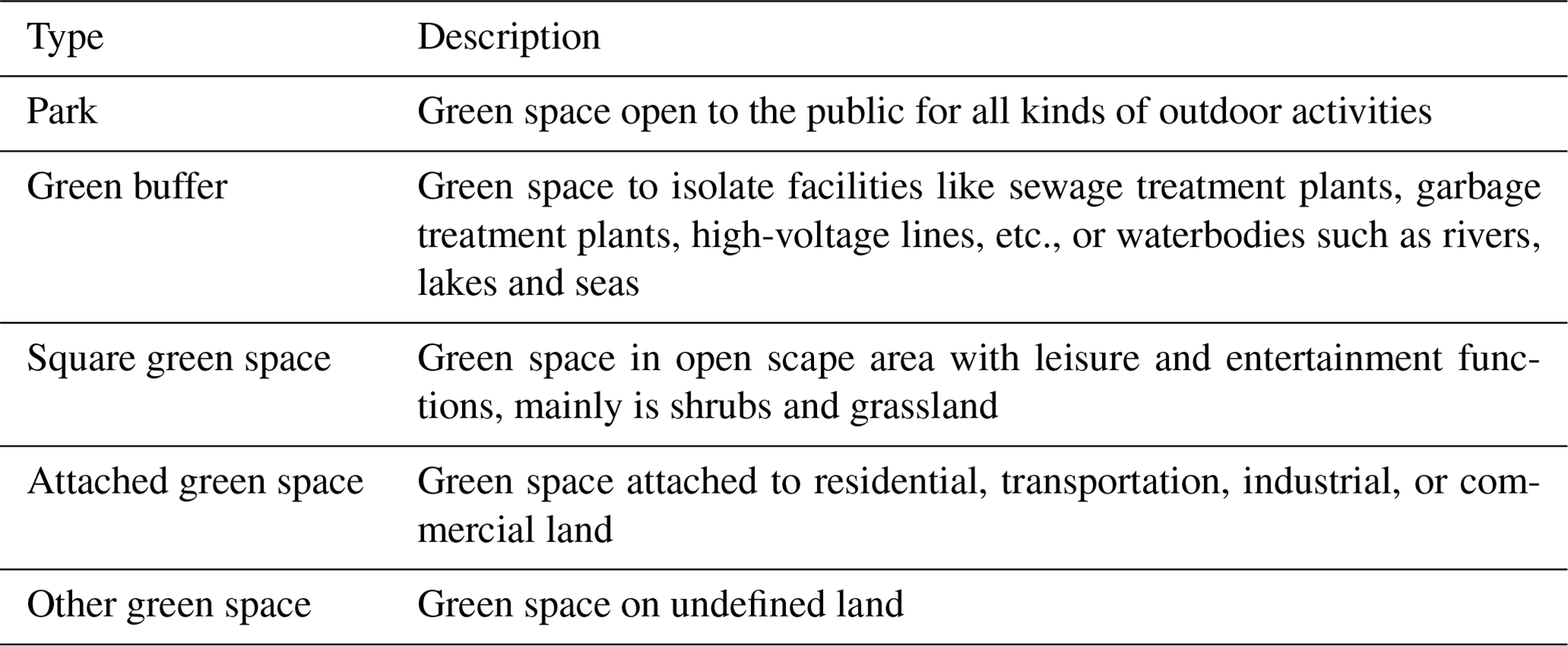
Urban green space can be divided into five categories, including parks, green buffers, square green spaces, attached green spaces, and other green spaces (W. Chen et al., 2018), as described in Table 1. Different types of UGS vary not only in their functions but also in shape and scale, which become more apparent in high-resolution images. For instance, parks and green buffers are often occurring in a relatively large volume, while attached green spaces and square green spaces are mainly scattered in urban areas in a smaller form. In other words, urban green space is not only diverse but also has large inter- and intra-class-scale differences. Therefore, a dataset that contains UGS samples of different types and scales is an important foundation for the model to learn and identify UGS accurately.
In order to provide an extensive sample database for wide-ranging UGS mapping and a benchmark for comparisons among deep learning algorithms, a large-scale, high-resolution urban green space dataset (UGSet) is constructed, which contains 4544 images of 512×512 in size and with a spatial resolution of nearly 1 m. These images are collected from 142 sample areas in Guangdong Province, China, as shown in Fig. 3, through the Gaofen-2 (GF2) satellite. The GF2 satellite is the first civilian optical remote sensing satellite developed by China, with a spatial resolution of about 1 m, which is equipped with two high-resolution 1 m panchromatic and 4 m multispectral cameras. With the aim to filter out green space in non-urban areas, the data from the global urban boundaries (GUBs; Li et al., 2020) of 2018 are used to mask the urban areas of each sample image. After that, all kinds of UGSs in the images are carefully annotated through expert visual interpretation before being cropped into 512×512 patches. As can be seen from Fig. 4, the categories of non-UGS and UGS in the ground truth are represented by 0 and 255, respectively. According to the ratio of , the UGSet is randomly divided into the training set, verification set, and test set.
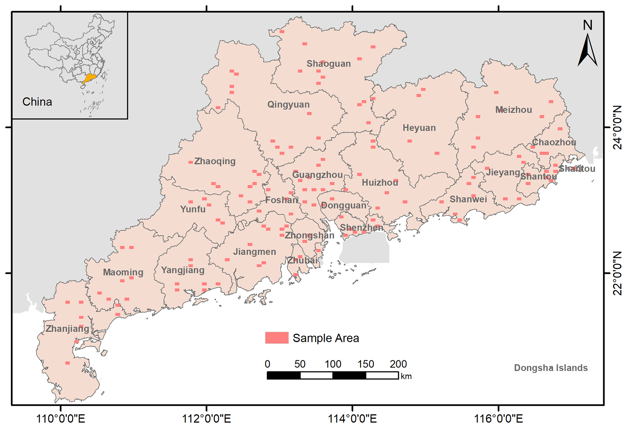
Figure 3The 142 sample areas in UGSet collected from Guangdong Province, China. Each sample area has a data frame of 3′45′′ in longitude and 2′30′′ in latitude.
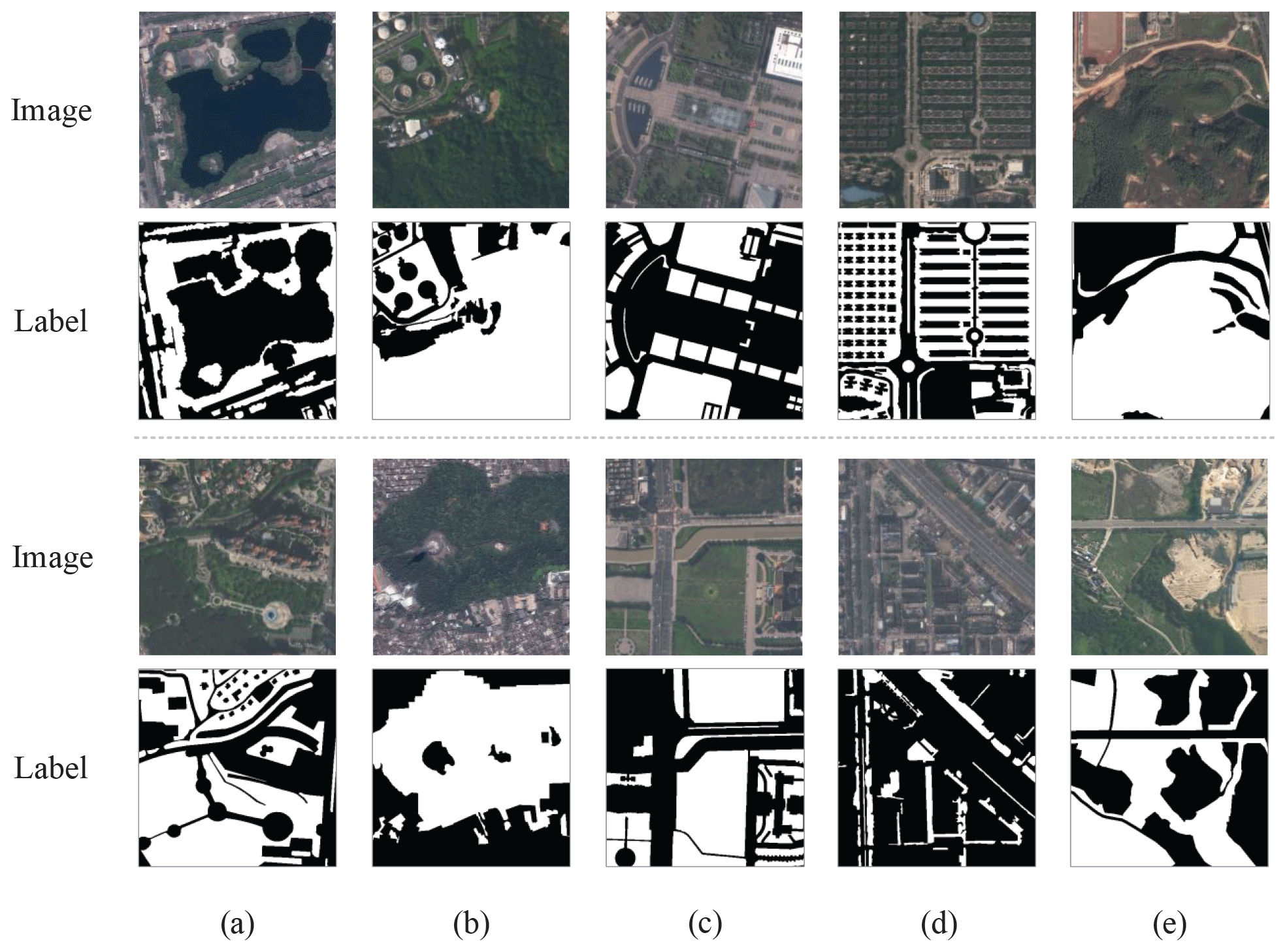
Figure 4Example of the image–label samples in UGSet. The images were retrieved from © Gaofen-2 2019. The first and third rows denote images of the samples, while the second and fourth rows provide corresponding labels for these images. Each column shows the different UGS types of samples, including (a) parks, (b) green buffers, (c) square green spaces, (d) attached green spaces, and (e) other green spaces.
2.2.2 Global urban boundaries (GUBs)
The data from the global urban boundaries (GUBs; Li et al., 2020) that delineate the boundary of global urban area in 7 years (i.e., 1990, 1995, 2000, 2005, 2010, 2015, and 2018) are obtained based on the 30 m global artificial impervious area (GAIA) data (Gong et al., 2020). It is worth noting that GAIA is the only annual map of impervious surface areas from 1985 to 2018 with a spatial resolution of 30 m. In this study, the GUB data in 2018 are adopted to mask the urban area. Specifically, in order to obtain accurate UGS samples, the GUB data are used to filter out non-relevant green space samples from non-urban areas. The GUB data are also applied to the UGS results from the model for post-processing, so as to obtain a final UGS map of each city.
2.2.3 Google Earth imagery
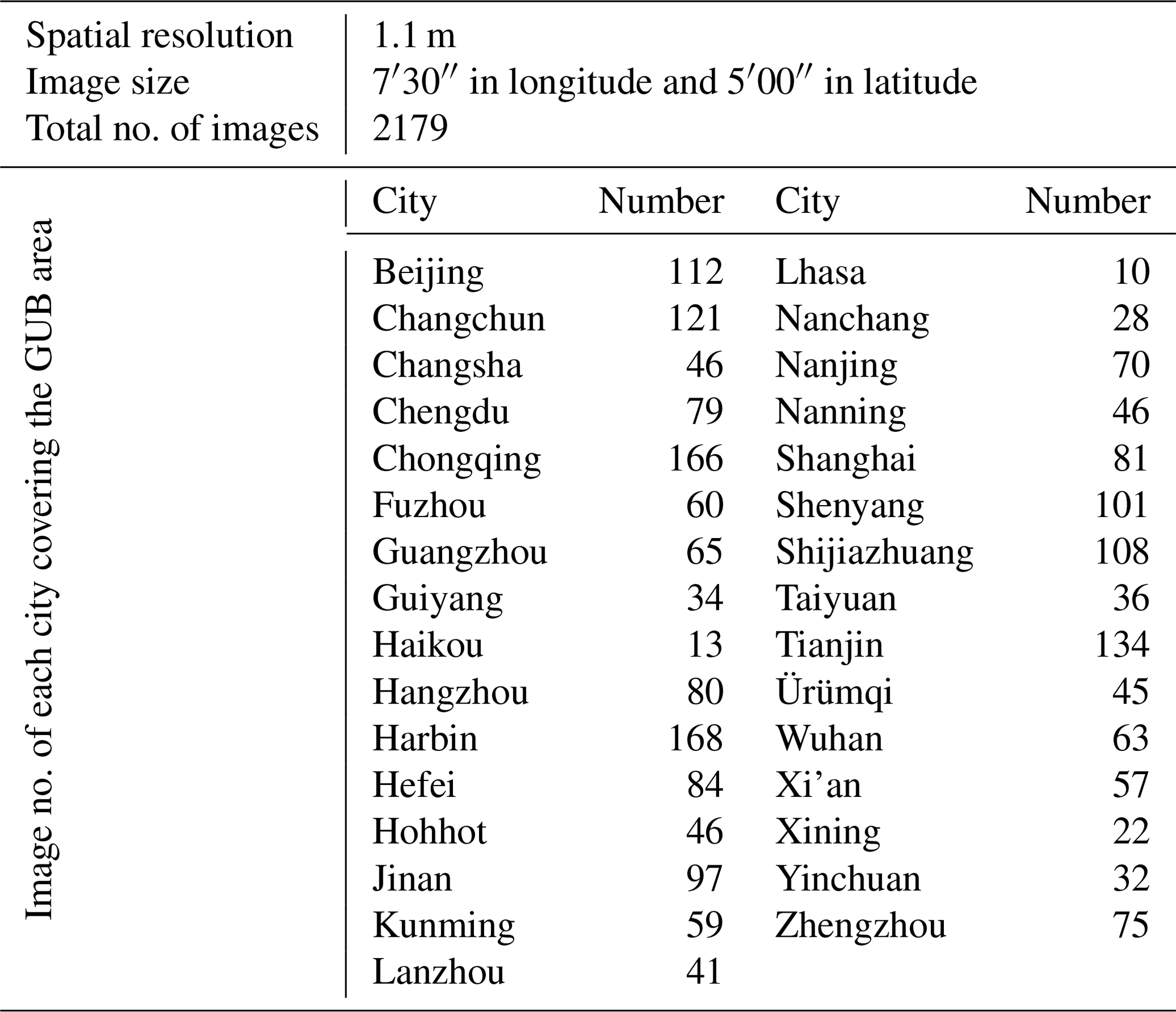
Google Earth is free software which enables users to view high-resolution satellite images around the world. Therefore, in order to obtain fine-grained UGS maps in the study area, a total of 2179 Google Earth images covering the GUB area of 31 major cities in China are downloaded, each with a data frame of 7′30′′ in longitude and 5′00′′ in latitude and a spatial resolution of nearly 1.1 m. In the download process, we give priority to the images of each data frame in 2020. However, if there is no clear and cloud-free image available for the data frame within the selected period, then we can only download the image from the adjacent date as a replacement. Limited by the GPU (graphics processing unit) memory, these images are all cropped to the size of 512×512 for prediction. The statistical description of the Google Earth imagery is summarized in Table 2. All of the Google Earth images can be accessed through the dataset link, together with the UGS-1m product.
In order to realize large-scale and fine-grained UGS mapping, a general model framework is essential, in addition to a sufficiently large dataset. Therefore, we propose a deep learning framework for UGS mapping; its flowchart is shown in Fig. 5. Inspired by adversarial domain adaptation frameworks (Tsai et al., 2018), the proposed framework includes a generator and a discriminator. In particular, a fully convolutional neural network, namely UGSNet, is designed as the generator for learning and extracting fine-grained UGS information. On the other hand, a simple, fully connected network is employed as the discriminator to help with model domain adaptation and achieve large-scale UGS mapping.

Figure 5Flowchart of the proposed deep learning framework for UGS mapping. The images in the UGSet were retrieved from © Gaofen-2 2019, while the images of the target city are from © Google Earth 2020). The red dashed lines denote the loss of back-propagation for model optimization. Lugs, LD, and Ladv represent the segmentation loss, the discrimination loss, and the adversarial loss, as described in Sect. 3.3.
The following (Sect. 3.1 and 3.2) will introduce the structure of UGSNet and discriminator, respectively. The optimization process of the deep learning framework will be described in Sect. 3.3, which can be divided into two parts, i.e., pre-training and adversarial training. Parameter settings and accuracy evaluation will be covered in Sect. 3.4 and 3.5.
3.1 UGSNet
The UGSNet contains two parts, namely a backbone to extract multi-scale features and generate coarse results and a point head module to obtain fine-grained results.
3.1.1 Backbone
The structure and elements of the backbone are shown in Fig. 6, which adopts the efficient ResNet-50 (He et al., 2016) as a feature extractor to capture multi-scale features from the images. This segment contains five stages, where the first stage consists of a 7×7 convolutional layer, a batch normalization layer (Ioffe and Szegedy, 2015), a rectified linear unit (ReLU) function (Glorot et al., 2011), and a max-pooling layer with a stride of 2. Then, four residual blocks (ResBlock) are utilized to capture deep features of four different levels. The four ResBlocks are connected by four enhanced coordinate attention (ECA) modules to enhance feature representations.

Figure 6Architecture of the backbone in UGSNet. The image was retrieved from © Gaofen-2 2019. (a) Backbone overview. (b) Sketch diagram of the ResBlock. (c) ECA module.
Previous researchers have proved that attention mechanism can bring gain effects to deep neural networks (Vaswani et al., 2017; Woo et al., 2018). Recently, a novel coordinate attention (CA; Hou et al., 2021) was proposed, which improved the weakness of traditional attention mechanisms in obtaining long-range dependence by embedding location information efficiently. Specifically, in order to capture the spatial coordinate information in the feature maps, the CA uses two 1-dimensional (1D) global pooling layers to encode input features along the vertical and horizontal directions, respectively, into two direction-aware feature maps. However, this approach ignores the synergistic effect of features in two spatial directions. Therefore, we propose the enhanced coordinated attention (ECA) modules. In addition to the original two parallel 1D branches encoding long-distance correlation along the vertical and horizontal direction, respectively, ECA also introduces a 2D feature-encoding branch to capture the collaborative interaction of feature maps in the entire coordinate space, so as to obtain more comprehensive, coordinate-aware attention maps for feature enhancement. The structure of the ECA module is shown in Fig. 6c.
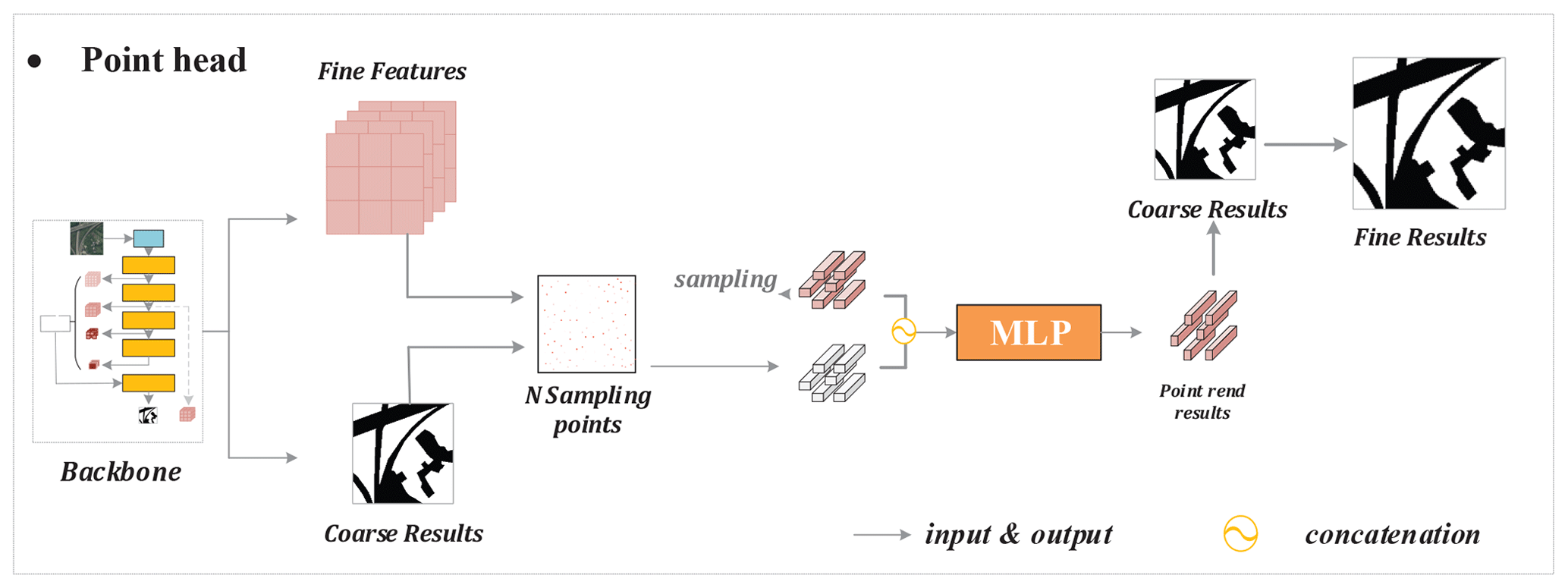
Figure 7Structure of the point head in UGSNet. The image in the backbone was retrieved from © Gaofen-2 2019. Given the fine features and the coarse UGS results from the backbone, the point head will firstly collect N(=1024) sampling points with the lowest certainty to construct point-wise features, which will be input into a multilayer perceptron (MLP) for classification and help obtain fine UGS results.
Then, four 1×1 convolutional blocks will be applied to the attention-refined features by the ECA modules to unify their output channels to 96. Then, they are concatenated together after being resized. Finally, the fused features will be input into two 3×3 convolutional layers to generate a coarse prediction map, which is one-quarter of the size of the input image.
3.1.2 Point head
Many semantic segmentation networks directly sample high-dimensional features to obtain the segmentation results of original image size, which will lead to rough results, especially near the boundary. Therefore, the point head is introduced into UGSNet, which uses the point-rending strategy (Kirillov et al., 2020) to obtain fine-grained UGS results efficiently. According to Fig. 7, given the fine-grained features and the coarse UGS results from the backbone, the specific process in the point head includes the following three steps: (1) first, collect N sampling points with lower certainty. (2) Then, construct the point-wise features of the selected N points based on the coarse UGS results and fine-grained features from the backbone. (3) Finally, reclassify the results of the selected N points through a simple multilayer perceptron (MLP). Detailed information of each step will be elaborated in the following.
In the first step, how to adaptively select sample points is the key to improving the segmentation results in an efficient and effective way, so different sampling strategies are adopted in the training and inference process. At the training stage, different points are expected to be taken into account. Therefore, at first k×N points will be randomly generated from the coarse segmentation results as candidates; then, β×N () points with the highest uncertainty will be selected from the k×N ones. After that, the other points will be randomly selected from the remaining candidates. In the inference process, the N sampling points are directly selected from the candidate points with highest uncertainty to consider more hard points. The second step is to build point-wise features based on the N sampling points obtained in the previous step. The coarse prediction and the selected fine-grained features from the backbone (the output of ResBlock-2 in this paper) corresponding to each sampling point will be concatenated to obtain point-wise features, so that the feature can contain both local details and the global context. Finally, the point-wise features will input into an MLP, which is actually a 1×1 convolutional layer, to obtain new classification results for each point. In our experiments, N=1024 sampling points will be collected, and the values of k and β are 3 and 0.75, respectively.
3.2 Discriminator
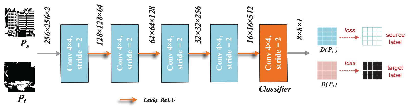
In order to transfer the prior knowledge from UGSet to images from other regions, a discriminator is adopted to obtain a well-adapted UGSNet for each city in an unsupervised way. As shown in Fig. 8, the discriminator consists of five convolutional layers with a kernel size of 4 and a stride of 2, each connected by a leaky ReLU layer. The output channels of each convolutional layers are 64, 128, 256, 512, and 1, respectively. Given an input of the softmax prediction map from the generator, , the discriminator will output a discriminant result of the input, . After that, the discriminator will optimize itself according to the discrimination accuracy through the cross-entropy loss in Eq. (5).
3.3 Optimization
The training of the proposed deep learning framework can be divided into two steps, namely pre-training and adversarial training. At the beginning, the UGSNet will be fully trained on UGSet to obtain the initial parameters for the generator. After that, the discriminator will be adopted to help generalize the pre-trained UGSNet to different target cities through adversarial learning. Detailed information on the optimization process is described in the following.
3.3.1 Pre-training
In the pre-training process, the UGSNet will learn the characteristics of all kinds of UGS from UGSet. Let us suppose that the coarse result output by the backbone is X and that the ground truth is Y. Then, the loss between Y and X is calculated by a dice loss, which can be defined as follows:
where is the intersection between X and Y, while and denote the number of elements of X and Y, respectively.
The loss of the classification results of the N sampling points in the point head is measured by the cross-entropy loss, which can be defined as follows:
where xi and yi represent the results and ground truth of the ith point among the N sampling ones, respectively.
Finally, the UGSNet is optimized by a hybrid loss, which can be expressed by the following:
3.3.2 Adversarial training
After pre-training, the UGSNet is employed as the generator in the deep learning framework and is trained with the discriminator to obtain a model that can be used for the UGS extraction of a target city. Taking the image Is and ground truth Ys in UGSet and the image It from the target city as input, the adversarial training process requires no additional data for supervision, which can be summarized as follows:
-
We take the pre-trained UGSNet as the starting training point of the generator, so that Is and It are forwarded to the generator G to obtain their prediction results of Ps and Pt, which can be denoted as follows:
-
We input Ps and Pt into the discriminator D in turn to distinguish the source of the inputs.
-
According to the judgment result, the discriminator D will be optimized first, which can be denoted as follows:
where y represents the source of the inputs, y=0 denotes an input P of Pt, and y=1 denotes an input of Ps.
-
Then, an adversarial loss Ladv is calculated to help promote the generator G to produce more similar results to confuse the discriminator. The Ladv is actually the loss when the discriminator D misclassifies the source of Pt as Is, which can be expressed as follows:
-
Finally, the generator will be optimized through the following objective function:
3.4 Parameter settings
During the pre-training process, the training set of the UGSet is used for parameter optimization, while the verification set was used to monitor the training direction and save the model in time. Five common semantic segmentation models are selected for comparison to prove the validity of UGSNet, including U-Net (Ronneberger et al., 2015), SegNet (Badrinarayanan et al., 2017), UPerNet (Xiao et al., 2018), BiSeNet (Yu et al., 2018), and PSPNet (Zhao et al., 2017). In addition, an ablation study is also conducted to further verify the effectiveness of the ECA modules and the point head. All models are fully trained for 200 epochs based on the Adam optimizer, with an initial learning rate of 0.0001, which begins to decline linearly in the last 100 epochs. A batch size of eight sample pairs is adopted due to the limitation on GPU memory. Data augmentation was applied during model training, including cropping, random rotation, and flipping. Specifically, cropping refers to randomly clipping an area of 256×256 size from the input sample of size 512×512. Rotation refers to randomly rotating the sample at a random angle within the range of [−30∘, 30∘] in the proportion of 20 %. Flipping refers to a mirror flip of samples from four different angles (up, down, left, and right) with a probability of 30 %. After training, all selected models were compared on the test set. The adversarial training process lasts for 10 000 epochs, in which the batch size is set to 2. Both the generator and the discriminator employ an initial learning rate of 0.0001. All experiments are implemented in PyTorch environments and are conducted in GeForce RTX 2080 Ti to accelerate model training.
3.5 Accuracy evaluation
Five indices are involved in the evaluation, including precision (Pre), recall (Rec), F1 score, intersection over union (IoU), and overall accuracy (OA). Suppose that TP, FP, TN, and FN refer to the true positive, false positive, true negative, and false negative, respectively. These indices can be defined as follows:
During the pre-training process, Pre, Rec, F1, and IoU are utilized to measure the model performance on UGSet, which is commonly used in semantic segmentation tasks. In the process of verifying the accuracy of the generated UGS maps (UGS-1m), Pre, Rec, F1 and OA are employed.
4.1 Accuracy evaluation on UGS-1m
Figure 9 provides an overview of UGS-1m product, which can be downloaded from https://doi.org/10.57760/sciencedb.07049 (Shi et al., 2023). In order to show the detailed information of the UGS-1m, two groups of magnified snapshots are also provided in Figs. 10 and 11. It can be seen that the results of UGS-1m are consistent with the green space in the image, no matter which of the three developed municipalities in Fig. 10 or the three capital cities in development in Fig. 11 are evaluated. While these comparisons can initially display the good visualization effect of UGS-1m, the accuracy evaluation is also conducted to further test it from a quantitative perspective. Since there is no large-scale and fine-grained UGS ground truth for an accuracy evaluation, five different cities are selected to evaluate the reliability of the UGS results in the UGS-1m, including Changchun, Beijing, Wuhan, Guangzhou, and Lhasa, as shown in Fig. 12. In total, 17 sample tiles are collected from the five cities, among which Changchun, Beijing, and Guangzhou each contribute four tiles. Due to the relatively small built-up areas, three and two tiles are collected from Wuhan and Lhasa, respectively. The UGS annotations of all tiles are obtained by expert interpretation. The accuracy evaluation is conducted between the annotated reference map and the result in UGS-1m.

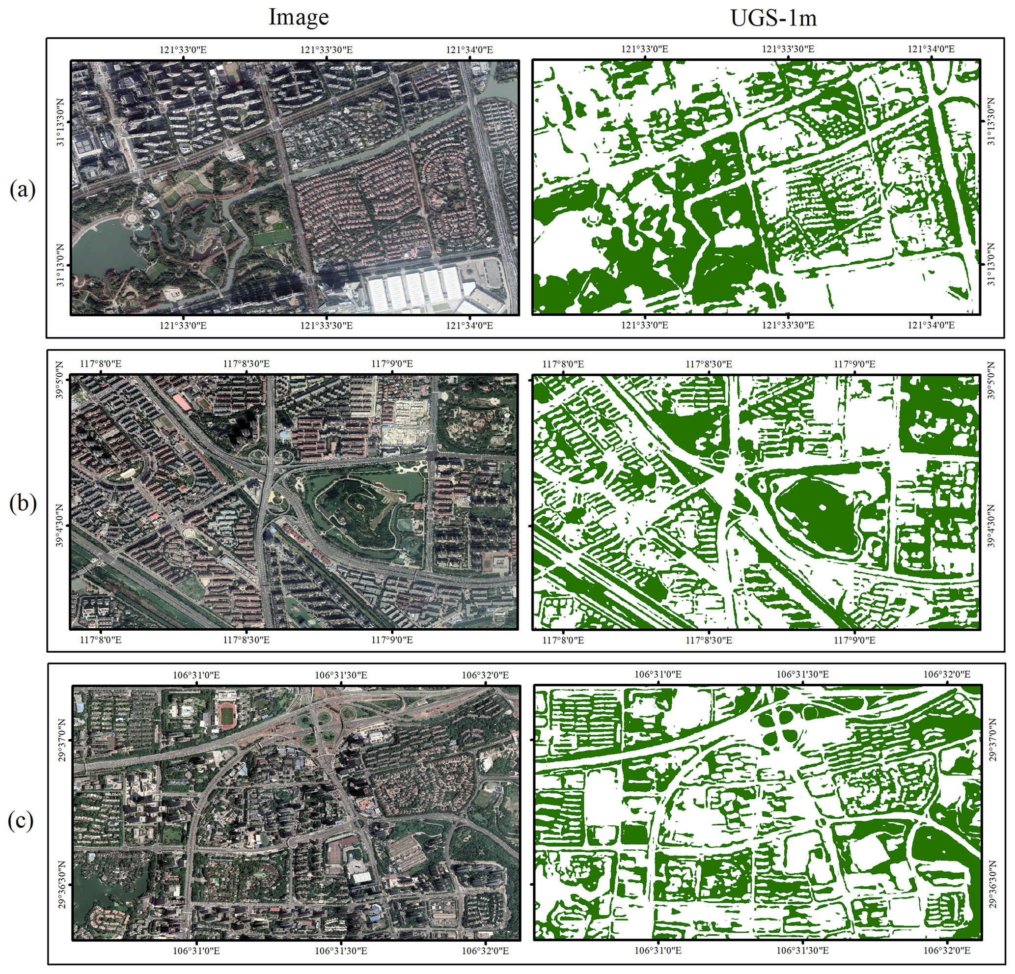
Figure 10Detailed UGS results in UGS-1m from three municipalities. Images are from © Google Earth 2020. (a) Shanghai. (b) Tianjin. (c) Chongqing.
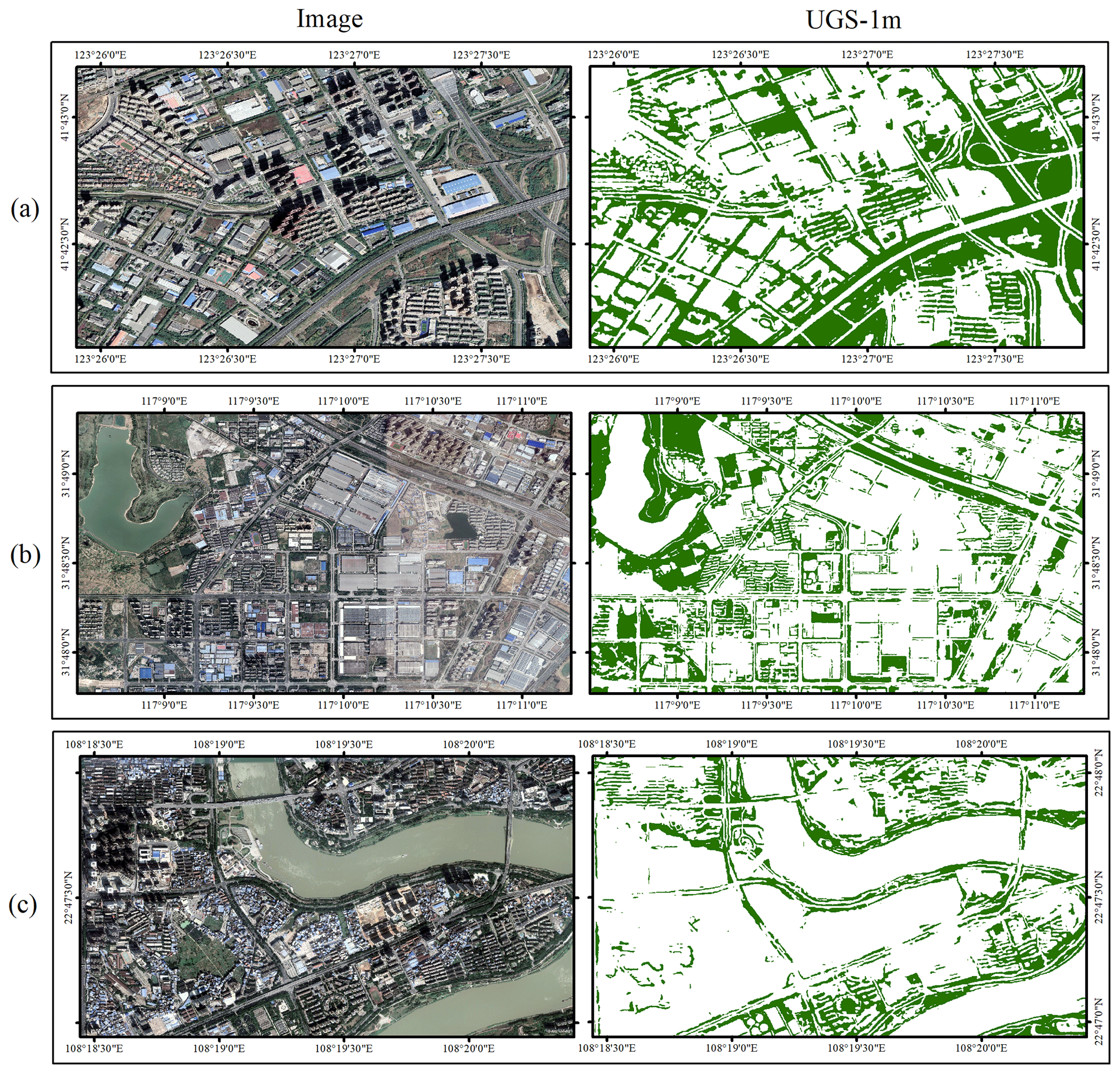
Figure 11Detailed UGS results in UGS-1m from three capital cities. Images are from © Google Earth 2020. (a) Shenyang. (b) Hefei. (c) Nanning.

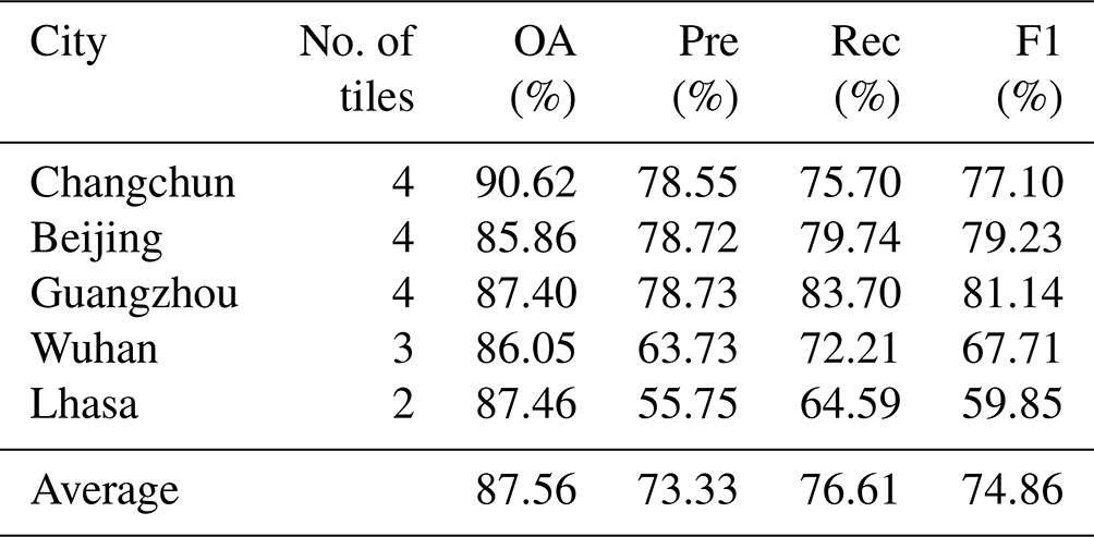
The evaluation results are summarized in Table 3, which are evaluated by OA, Pre, Rec, and F1. It can be seen that, in the five cities for verification, the average OA of all cities is 87.56 %, while the OA of each city is higher than 85 %. Among them, the highest OA is 90.62 % in Changchun, while the lowest OA also reaches 85.86 % in Beijing, indicating that the UGS results in different cities are basically good. In terms of the F1 score, Guangzhou has the highest F1 score of 81.14 %, followed by Beijing and Changchun with 79.23 % and 77.10 %, respectively. Though the F1 scores of Wuhan and Lhasa are relatively low, at 67.71 % and 59.85 %, respectively, the average F1 score of the final UGS results also reaches 74.86 %. Moreover, the average Rec of 76.61 % also denotes a relatively low missed-detection rate of the UGS extraction results, which is significantly important in applications. In general, after quantitative validation in several different cities, the availability of UGS-1m is preliminarily demonstrated.
4.2 Qualitative analysis on UGS-1m
The qualitative analysis is carried out in this section to further analyze the performance of UGS extraction and its relationship with external factors, such as geographical location, UGS types, phenological phase, etc. Therefore, visualization comparisons conducted in three cities, including Changchun, Wuhan, and Guangzhou, are displayed in Figs. 13–15.
From the overview image of Changchun (Fig. 13) and Guangzhou (Fig. 14), it can be seen that the extracted UGS results are in good agreement with the reference maps, which is mainly reflected in the good restoration of UGS at various scales in each example image. The magnified area of each image further shows the details of UGS-1m for extracting different kinds of UGS, including parks, squares, green buffers, and attached green spaces. Specifically, the UGS-1m performs well in the extraction of green spaces attached to residential buildings, although they are complex and broken in morphology compared to other UGS types. Notably, though Changchun and Guangzhou are geographically far away, distributed in the northernmost and southernmost regions of China, respectively, the UGS results in these two cities are both good. This shows that the performance of the proposed UGS extraction framework is unlikely to be affected by the difference in geographical location, which may attributed to the adversarial training strategy to help model adaptation.
The visualization result of Wuhan is further provided in Fig. 15 for analysis. It can be seen that the UGS results in Wuhan are mainly influenced by the shadows of buildings. On the one hand, the UGS features are sometimes blocked by building shadows, resulting in relatively poor extraction effect, such as the magnified area in Fig. 15b. On the other hand, the building shadows can easily be extracted as attached green space, according to Fig. 15c. This shows that the result of green space extraction is related to the angle of the image taken. When the angle is larger, it is more likely to have building shadows in the image, thus affecting the subsequent UGS extraction, especially the green space that is attached to buildings. In addition, the results are also affected by the phenological phase, as shown in Fig. 15a. On the whole, the UGS with a higher and denser vegetation canopy is easier to identify accurately, and on the contrary, the lower and sparser UGS is more easily misclassified due to the similar appearance with other land types, such as bare land.
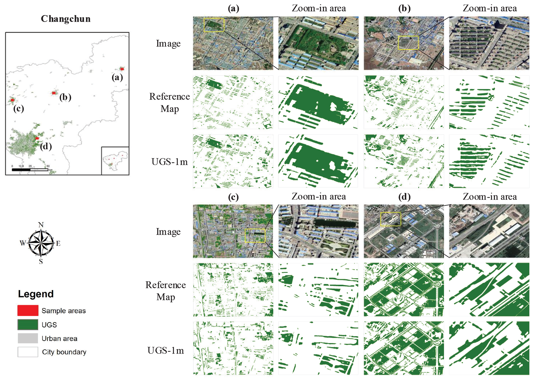
Figure 13Qualitative analysis in UGS-1m, with a case study in Changchun city. Panels (a)–(d) are four example areas collected from Changchun. Images are from © Google Earth 2020.
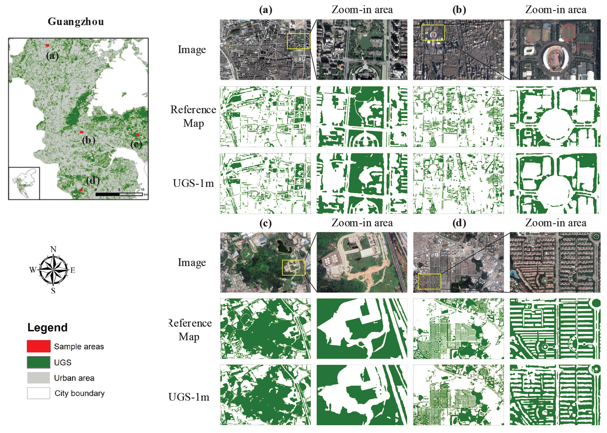
Figure 14Qualitative analysis in UGS-1m, with a case study in Guangzhou city. Panels (a)–(d) are four example areas collected from Guangzhou. Images are from © Google Earth 2020.

Figure 15Qualitative analysis in UGS-1m, with a case study in Wuhan city. Panels (a)–(c) are three example areas collected from Wuhan. Images are from © Google Earth 2020.
4.3 Comparison with existing products
We compare the UGS-1m results with the existing global land cover products to verify the reliability of the results, including GlobeLand30 (Chen and Chen, 2018), GLC_FCS30 (Zhang et al., 2021), and Esri 2020 LC (© 2021 Esri). Due to different classification systems, these products need to be reclassified into two categories. Specifically, forests, grasslands, and shrublands are reclassified as UGS, while the other categories are reclassified as non-UGS. Examples from six different cities in different geographical locations, including Changchun, Ürümqi, Beijing, Chengdu, Wuhan, and Guangzhou, are collected to give more comprehensive demonstrations of our UGS results. The visualization comparison among UGS-1m, GlobeLand30, GLC_FCS30, and Esri 2020 LC is shown in Fig. 16. Apparently, the three comparative products contain most large-scale UGS, among which the GlobeLand30 performs best with the most complete UGS prediction. However, many detailed UGS features are still missed due to the limitation in the spatial resolution of the source image. Remarkably, the UGS-1m provides UGS with a relatively large scale and detailed UGS information such as attached green spaces. The results and comparisons fully demonstrate the effectiveness and potential of the proposed deep learning framework for large-scale and fine-grained UGS mapping.
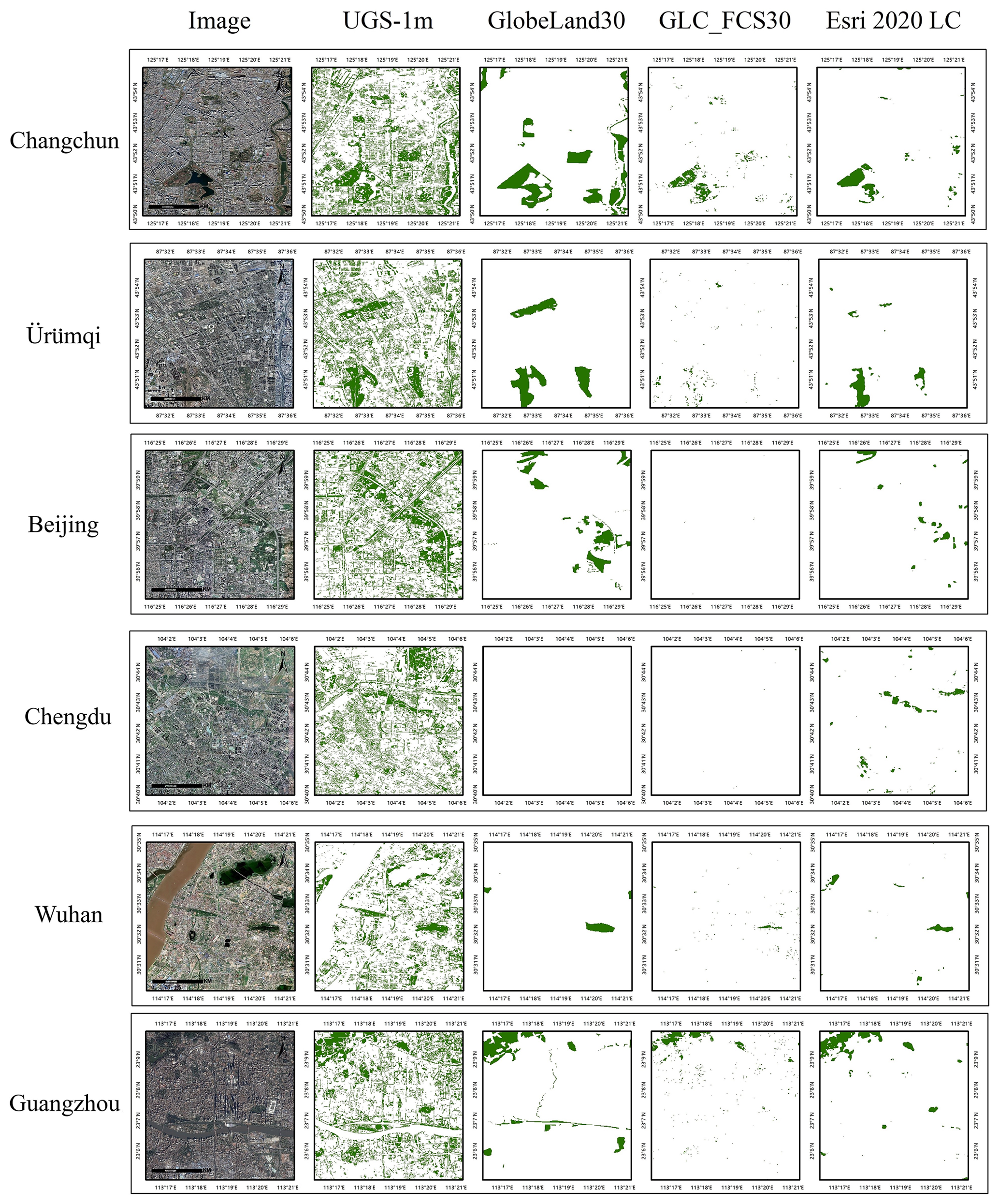
Figure 16Visualization comparisons between UGS-1m, GlobeLand30 (Chen and Chen, 2018), GLC_FCS30 (Zhang et al., 2021), and Esri 2020 LC (© 2021 Esri). Images are from © Google Earth 2020.
4.4 UGS statistics and analysis based on UGS-1m
While the previous evaluations and comparisons have proved the advantages and validity of the UGS-1m, this section will explore the potential utility of the UGS-1m product. As mentioned in the introduction, green space equality is critical for achieving the Sustainable Development Goals, and this requires fine-grained distributions of UGS as basic data. At this point, compared with the traditional Statistical Yearbook data, our UGS-1m product can provide relatively objective and more detailed information about the distribution of green space. Therefore, statistics are conducted on the UGS-1m data to obtain particular information of each city, including the UGS area and the UGS rate in the GUB area, which are summarized in Table 4.
As shown in Table 4, the UGS area of the different cities varies greatly. For example, it is seen that the UGS area of Beijing is the largest among all 31 cities studied, reaching 1021.55 km2, while that of Lhasa is the smallest, with only 11.41 km2. The statistical information on the UGS area indicates that UGS-1m can provide a quick and intuitive comparison of the stock of UGS in different cities. However, a small UGS area does not always mean a lack of green space because the urban area needs to be considered at the same time. Therefore, the UGS rate in the GUB area is further calculated to measure the volume and distribution of green space in different cities. At this time, it can be seen that Yinchuan has the highest UGS rate, accounting for 25.35 %, while Beijing, which has the largest UGS area, has a slightly lower UGS rate of 20.74 %. Besides, the UGS rate of 9.27 % in Lhasa, which has the least UGS area, is also slightly better than that of Lanzhou, which has the lowest UGS rate of 8.64 %. The results and comparisons further show that the shortage and imbalance of green space cannot be reflected only from the perspective of the stock of green space, and more information is often needed for a more comprehensive analysis.
The above statistical analysis only shows the most simple and intuitive applicability of UGS-1m as a large-scale and refined green space product, but it is far more than that. Since the high-resolution UGS-1m can provide a detailed distribution of green space, it provides a possibility for much more research under fine-grained scenarios. When considering different datasets or materials, more comprehensive information of UGS can be obtained. For example, by combining high-resolution population (e.g., WorldPop data; Tatem, 2017) with UGS-1m, the availability of residents to green space can be measured, that is, green space equity. Or, when combined with the distribution of urban villages and formal housing spaces, their differences in the green landscape pattern can be studied. We also hope to explore these research areas in the future.
Table 4Statistical results of UGS-1m in the UGS area and rate for 31 major cities in China.
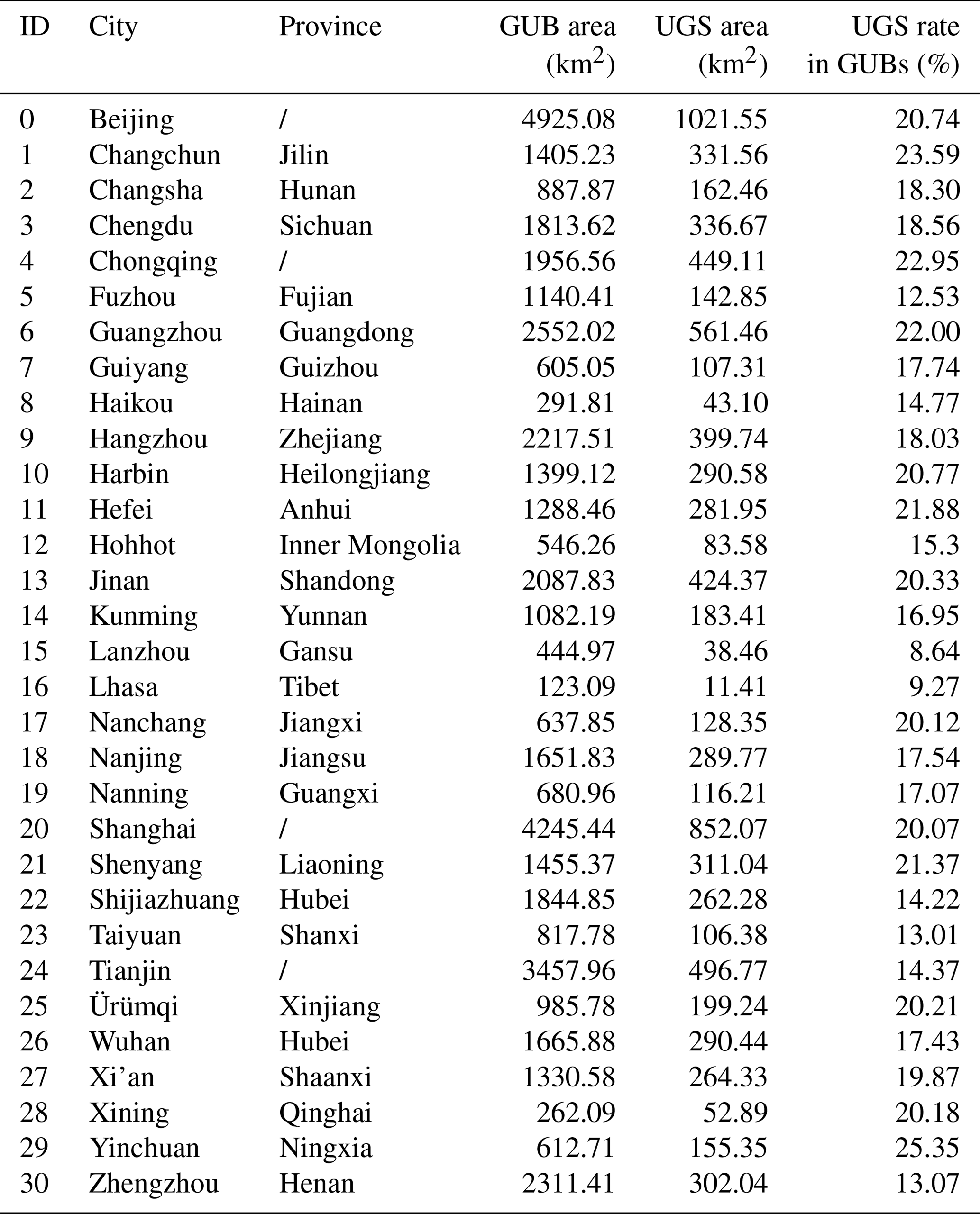
The forward slash in the province column denotes a municipality city.
5.1 Comparative experiments at pre-training stage
As mentioned above, before the start of adversarial training stage, the generator will be initialized by a pre-trained UGSNet on UGSet. Therefore, in order to fully verify the advancement of UGSNet and its qualification to initialize the generator, this section introduces several state-of-the-art (SOTA) deep learning models as candidate generators for comparison. Note that the comparative experiment is completely conducted on UGSet, and no discriminator is introduced. After all the models have been fully trained on training set of the UGSet, the best-trained parameters of each model will be evaluated on the testing set of the UGSet. The comparative results are provided in Table 5.
As Table 5 shows, the proposed UGSNet outperforms all SOTA baselines with the highest F1 score and IoU of 77.30 % and 62.99 %, respectively. The second-ranked PSPNet obtains an IoU of 60.96 %, which is 2.03 % lower than that of UGSNet. The ablation study indicates that the integration of the ECA modules and point head can improve the base model by 0.17 % and 0.69 % on IoU, respectively, which proves their effectiveness on UGS extraction. The IoU of UGSNet is 1.22 % higher than that of the base model, indicating that the combination of ECA modules and point head has a greater gain effect. The quantitative results demonstrate the validity of UGSNet.
Figure 17 further demonstrates the performance of different methods on different kinds of UGS. It can be seen that, after fully training on the UGSet dataset, each model can identify the approximate region of various green spaces, including SegNet, which has shown poor performance in the quantitative comparisons. Therefore, the superiority of the green space identification results is mainly reflected in two aspects. One aspect is the ability to extract the UGSs of great inter-class similarity. As shown in the first row of Fig. 17, the UGSNet can accurately identify the yellow box area, in which the green space of a park has confused most comparative methods. Another aspect is the capability to grasp fine-grained edges, especially for small-scale UGS, such as the attached UGS in the last row of Fig. 17.
Table 5Performance of the different semantic segmentation methods in UGSet. The bold font represents the highest precision of each column.
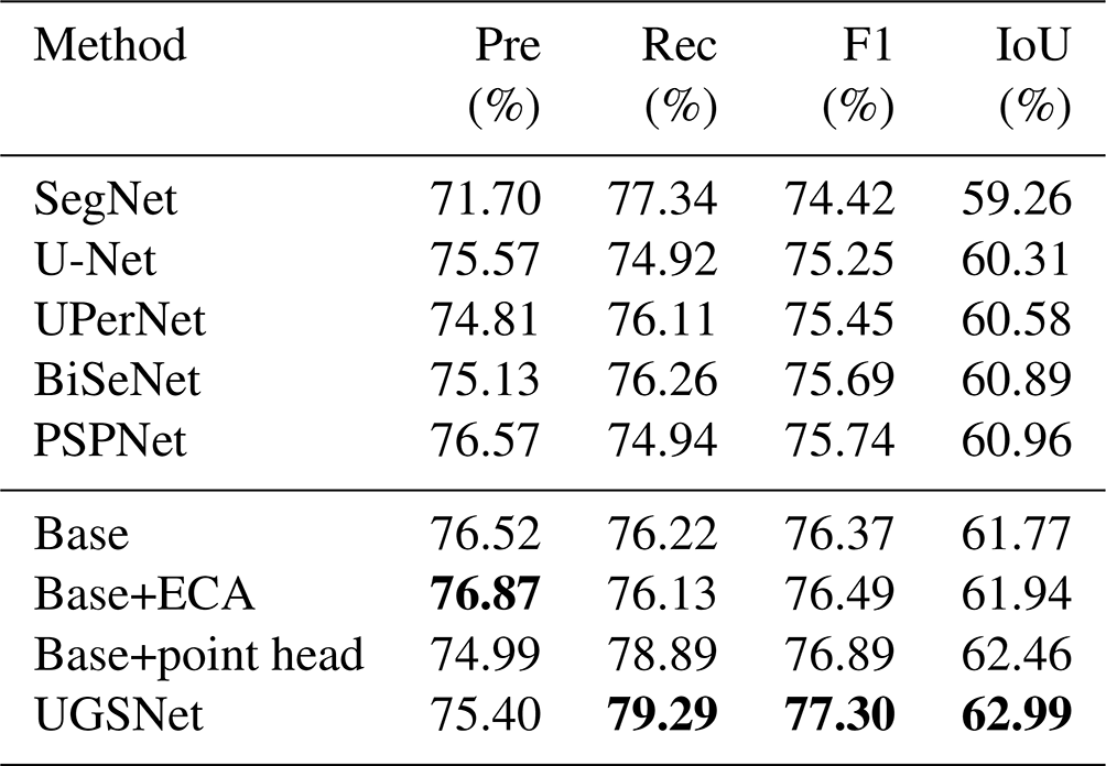
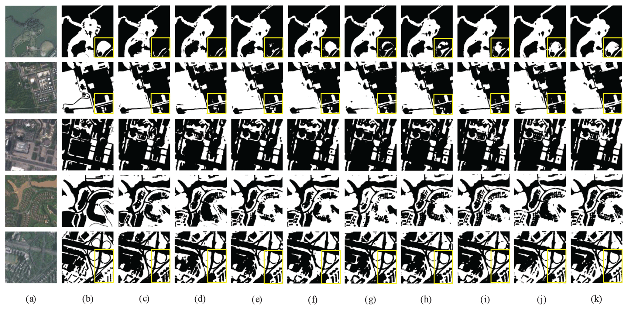
Figure 17Visualization comparisons of different methods in UGSet Images are from © Gaofen-2 2019. (a) Image. (b) Label. (c) SegNet. (d) U-Net. (e) UPerNet. (f) BiSeNet. (g) PSPNet. (h) Base. (i) Base+ECA. (j) Base+point head. (k) UGSNet.
5.2 Ablation study on the discriminator
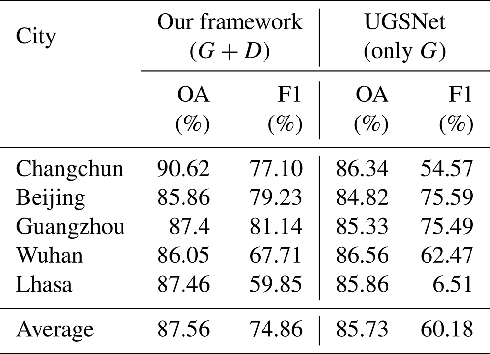
As we have mentioned above, the proposed framework is composed of a generator and a discriminator, which adopts the adversarial training to help the model transfer learning. In order to test the effectiveness of the proposed framework, this section further conducted ablation experiments with and without the discriminator, which, respectively, correspond to the following:
-
Our framework (G+D) contains a generator and a discriminator, in which the generator is initialized by the UGSNet pre-trained on UGSet, and the discriminator is employed at the adversarial training stage to overcome domain shifts and obtain a refined UGSNet for each target city before generating the UGS map for it.
-
UGSNet (only D) has no discriminator involved and simply applies the pre-trained UGSNet to each target city/area and generates their UGS maps, regardless of the domain shifts between the UGSet and images from different target cities/areas.
The result of our framework (G+D) comes from quantitative results of UGS-1m in Sect. 4. In order to test the effect of UGSNet (only G), the pre-trained UGSNet is applied to the same sample areas for accuracy evaluation. The final ablation results are shown in Table 6. It can be seen from the results that, when the discriminator is not used, the OA of almost all cities decreases to a certain extent. Generally speaking, the average OA decreases from 87.56 % to 85.73 %. The F1 score shows a sharp decline, with the average F1 score dropping from 74.86 % to 60.18 %. Specifically, the decline in the F1 score in Guangzhou and Beijing is relatively small. It indicates that domain shifts between the images of these two cities and the UGSet images are not that significant, so the pre-trained model can still have a better performance. It is worth noting that the use of discriminator can significantly improve the results in Changchun, according to the great growth of the F1 score of 22.53 %. Moreover, the results in Lhasa only have an F1 score of 6.51 % without D, which can reach 59.85 % when using D. The ablation experiment fully proves the effectiveness and potential of the proposed framework for large-scale green space mapping.
5.3 Limitations and future work
At present, the availability of high-resolution images is still severely limited by factors such as temporal resolution, image distortion, and cloud occlusion. Therefore, it is hard to collect all the Google Earth images used to generate UGS-1m in the same period, making it difficult to keep the unity of phenology. In the proposed deep learning framework, we introduce a domain adaptation strategy to deal with this problem to some extent. A comparison of the results has shown the effectiveness of UGS-1m and the feasibility and potential of the proposed deep learning framework for large-scale, high-resolution mapping. However, the current DL techniques still have limitations. In view of the spatial and spectral diversity of high-resolution remote sensing images, we have not been able to fully evaluate the domain adaptation effect of the adversarial framework for all heterogeneous images with different dates and resolutions. With the emergence of more and more high-resolution satellite images, the adversarial learning of multi-source images remains to be explored. Future works will be dedicated to extracting UGS information based on data with higher temporal resolution, such as synthetic-aperture radar (SAR) images and unmanned aerial vehicle (UAV) images.
Besides, even though the UGSet has proven to be practicable for UGS mapping, we still have to point out that there may be a small number of missing labels in the dataset, especially for attached green spaces. As analyzed above, the extraction of attached green spaces can be more easily affected by external factors, like the angle of the image taken. This also affects the annotation process. Fortunately, despite the possible deficiencies, the DL model can still learn from a large number of accurate annotations and capture the characteristics of different types of green spaces due to the strong generalization ability. We still hope that, in the following work, more attempts can be made to deal with the problems of labeling and identifying hard UGS types.
The dataset can be downloaded from https://doi.org/10.57760/sciencedb.07049 (Shi et al., 2023), including the UGS-1m product, UGSet, and the involved imagery. The code for the deep learning framework is available at https://doi.org/10.5281/zenodo.7581694 (Liu, 2023).
In this paper, we propose a novel deep learning (DL) framework for large-scale UGS mapping and generate the fine-grained UGS maps for 31 major cities in China (UGS-1m). The accuracy evaluation of the UGS-1m product indicates its reliability and applicability. Comparative experiments conducted on UGSet among several SOTA semantic segmentation networks show that UGSNet can achieve the best performance on UGS extraction. The ablation study on UGSNet also demonstrates the effectiveness of the ECA module and point head. Comparisons between UGS-1m and existing land cover products have proved the validity of the proposed DL framework for large-scale and fine-grained UGS mapping. The achievements provided in this paper can support the scientific community for UGS understanding and characterization and pave the way for the development of robust and efficient methods to tackle the current limits and needs of UGS analysis in the technical literature.
QS conceptualized the paper, collected the resources, led the investigation, acquired the funding, and reviewed and edited the paper. ML curated the data, developed the methodology, validated the project, did the formal analysis, visualized the paper, and prepared the original draft. AM and XL reviewed and edited the paper.
The contact author has declared that none of the authors has any competing interests.
Publisher's note: Copernicus Publications remains neutral with regard to jurisdictional claims in published maps and institutional affiliations.
We gratefully acknowledge all data providers, whose data have been used in this study, and would like to thank Jianlong Li and Zeteng Li, for their help in data collection. We sincerely appreciate the editor and the two referees, for their constructive comments to improve the quality of the paper.
This study has been supported by the National Key R&D Program of China (grant no. 2022YFB3903402), by the National Natural Science Foundation of China (grant nos. 42222106 and 61976234), by the Centre for Integrated Remote Sensing and Forecasting for Arctic Operations (CIRFA) and the Research Council of Norway (RCN; grant no. 237906), and by the Visual Intelligence Centre for Research-based Innovation funded by the Research Council of Norway (RCN; grant no. 309439).
This paper was edited by David Carlson and reviewed by Robbe Neyns and one anonymous referee.
Badrinarayanan, V., Kendall, A., and Cipolla, R.: Segnet: A deep convolutional encoder-decoder architecture for image segmentation, IEEE T. Pattern Anal., 39, 2481–2495, https://doi.org/10.1109/TPAMI.2016.2644615, 2017. a, b
Cao, Y. and Huang, X.: A deep learning method for building height estimation using high-resolution multi-view imagery over urban areas: A case study of 42 Chinese cities, Remote Sens. Environ., 264, 112590, https://doi.org/10.1016/j.rse.2021.112590, 2021. a
Chen, B., Tu, Y., Wu, S., Song, Y., Jin, Y., Webster, C., Xu, B., and Gong, P.: Beyond green environments: multi-scale difference in human exposure to greenspace in China, Environ. Int., 166, 107348, https://doi.org/10.1016/j.envint.2022.107348, 2022a. a
Chen, B., Wu, S., Song, Y., Webster, C., Xu, B., and Gong, P.: Contrasting inequality in human exposure to greenspace between cities of Global North and Global South, Nat. Commun., 13, 1–9, 2022b. a
Chen, J. and Chen, J.: GlobeLand30: Operational global land cover mapping and big-data analysis, Sci. China Earth Sci., 61, 1533–1534, 2018. a, b
Chen, J., Cao, X., Peng, S., and Ren, H.: Analysis and applications of GlobeLand30: a review, ISPRS Int. J. Geo-Inf., 6, 230, https://doi.org/10.3390/ijgi6080230, 2017. a
Chen, L.-C., Zhu, Y., Papandreou, G., Schroff, F., and Adam, H.: Encoder-decoder with atrous separable convolution for semantic image segmentation, in: Computer Vision – ECCV 2018, edited by: Ferrari, V., Hebert, M., Sminchisescu, C., and Weiss, Y., Springer International Publishing, Cham, 833–851, https://doi.org/10.1007/978-3-030-01234-2_49, 2018. a
Chen, W., Huang, H., Dong, J., Zhang, Y., Tian, Y., and Yang, Z.: Social functional mapping of urban green space using remote sensing and social sensing data, ISPRS J. Photogramm. Remote, 146, 436–452, 2018. a
Daudt, R. C., Saux, B. L., and Boulch, A.: Fully Convolutional Siamese Networks for Change Detection, in: 2018 25th IEEE International Conference on Image Processing (ICIP), IEEE, 4063–4067, https://doi.org/10.1109/ICIP.2018.8451652, 2018. a
Deng, L. and Yu, D.: Deep Learning: Methods and Applications, Foundations & Trends in Signal Processing, 7, 197–387, 2014. a
De Ridder, K., Adamec, V., Bañuelos, A., Bruse, M., Bürger, M., Damsgaard, O., Dufek, J., Hirsch, J., Lefebre, F., Pérez-Lacorzana, J. M., Thierry, A., and Weber, C.: An integrated methodology to assess the benefits of urban green space, Sci. Total Environ., 334, 489–497, https://doi.org/10.1016/j.scitotenv.2004.04.054, 2004. a
Devlin, J., Chang, M., Lee, K., and Toutanova, K.: BERT: Pre-training of Deep Bidirectional Transformers for Language Understanding, CoRR, abs/1810.04805, http://arxiv.org/abs/1810.04805, 2018. a
Everingham, M., Eslami, S. A., Van Gool, L., Williams, C. K., Winn, J., and Zisserman, A.: The pascal visual object classes challenge: A retrospective, Int. J. Comput. Vision, 111, 98–136, https://doi.org/10.1007/s11263-014-0733-5, 2015. a
Fuller, R. A., Irvine, K. N., Devine-Wright, P., Warren, P. H., and Gaston, K. J.: Psychological benefits of greenspace increase with biodiversity, Biol. Lett., 3, 390–394, https://doi.org/10.1098/rsbl.2007.0149, 2007. a
General Office of the State Council, PRC: Guidelines on scientific greening, https://www.mee.gov.cn/zcwj/gwywj/202106/t20210603_836084.shtml, last access: 3 June 2021. a
Glorot, X., Bordes, A., and Bengio, Y.: Deep Sparse Rectifier Neural Networks, J. Mach. Learn. Res., 15, 315–323, 2011. a
Gong, P., Wang, J., Yu, L., Zhao, Y., Zhao, Y., Liang, L., Niu, Z., Huang, X., Fu, H., Liu, S., Li, C., Li, X., Fu, W., Liu, C., Xu, Y., Wang, X., Cheng, Q., Hu, L., Yao, W., Zhang, H., Zhu, P., Zhao, Z., Zhang, H., Zheng, Y., Ji, L., Zhang, Y., Chen, H., Yan, A., Guo, J., Yu, L., Wang, L., Liu, X., Shi, T., Zhu, M., Chen, Y., Yang, G., Tang, P., Xu, B., Giri, C., Clinton, N., Zhu, Z., Chen, J., and Chen, J.: Finer resolution observation and monitoring of global land cover: first mapping results with Landsat TM and ETM+ data, Int. J. Remote Sens., 34, 2607–2654, https://doi.org/10.1080/01431161.2012.748992, 2013. a
Gong, P., Li, X., Wang, J., Bai, Y., Chen, B., Hu, T., Liu, X., Xu, B., Yang, J., Zhang, W., and Zhou, Y.: Annual maps of global artificial impervious area (GAIA) between 1985 and 2018, Remote Sens. Environ., 236, 111510, https://doi.org/10.1016/j.rse.2019.111510, 2020. a
He, K., Zhang, X., Ren, S., and Sun, J.: Deep residual learning for image recognition, in: 2016 IEEE Conference on Computer Vision and Pattern Recognition (CVPR), 770–778, https://doi.org/10.1109/CVPR.2016.90, 2016. a
Helber, P., Bischke, B., Dengel, A., and Borth, D.: Eurosat: A novel dataset and deep learning benchmark for land use and land cover classification, IEEE J. Sel. Top. Appl. Earth Obs., 12, 2217–2226, https://doi.org/10.1109/JSTARS.2019.2918242, 2019. a
Hou, Q., Zhou, D., and Feng, J.: Coordinate Attention for Efficient Mobile Network Design, in: 2021 IEEE/CVF Conference on Computer Vision and Pattern Recognition (CVPR), 13708–13717, https://doi.org/10.1109/CVPR46437.2021.01350, 2021. a
Huang, C., Yang, J., Lu, H., Huang, H., and Yu, L.: Green spaces as an indicator of urban health: evaluating its changes in 28 mega-cities, Remote Sens., 9, 1266, https://doi.org/10.3390/rs9121266, 2017. a, b
Huang, C., Yang, J., and Jiang, P.: Assessing impacts of urban form on landscape structure of urban green spaces in China using Landsat images based on Google Earth Engine, Remote Sens., 10, 1569, https://doi.org/10.3390/rs10101569, 2018. a
Ioffe, S. and Szegedy, C.: Batch Normalization: Accelerating Deep Network Training by Reducing Internal Covariate Shift, CoRR, abs/1502.03167, http://arxiv.org/abs/1502.03167, 2015. a
Jun, C., Ban, Y., and Li, S.: China: Open access to Earth land-cover map, Nature, 514, 434–434, https://doi.org/10.1038/514434c, 2014. a
Kirillov, A., Wu, Y., He, K., and Girshick, R.: PointRend: Image Segmentation As Rendering, in: 2020 IEEE/CVF Conference on Computer Vision and Pattern Recognition (CVPR), 9796–9805, https://doi.org/10.1109/CVPR42600.2020.00982, 2020. a
Kong, F., Yin, H., James, P., Hutyra, L. R., and He, H. S.: Effects of spatial pattern of greenspace on urban cooling in a large metropolitan area of eastern China, Landscape Urban Plan., 128, 35–47, https://doi.org/10.1016/j.landurbplan.2014.04.018, 2014. a
Krizhevsky, A., Sutskever, I., and Hinton, G. E.: Imagenet classification with deep convolutional neural networks, Adv. Neur. In., 25, 1097–1105, 2012. a
Kuang, W. and Dou, Y.: Investigating the patterns and dynamics of urban green space in China's 70 major cities using satellite remote sensing, Remote Sens., 12, 1929, https://doi.org/10.3390/rs12121929, 2020. a
Kuang, W., Zhang, S., Li, X., and Lu, D.: A 30 m resolution dataset of China's urban impervious surface area and green space, 2000–2018, Earth Syst. Sci. Data, 13, 63–82, https://doi.org/10.5194/essd-13-63-2021, 2021. a
Li, X., Gong, P., Zhou, Y., Wang, J., Bai, Y., Chen, B., Hu, T., Xiao, Y., Xu, B., Yang, J., Liu, X., Cai, W., Huang, H., Wu, T., Wang, X., Lin, P., Li, X., Chen, J., He, C., Li, X., Yu, L., Clinton, N., and Zhu, Z.: Mapping global urban boundaries from the global artificial impervious area (GAIA) data, Environ. Res. Lett., 15, 094044, https://doi.org/10.1088/1748-9326/ab9be3, 2020. a, b, c, d, e
Liao, C., Dai, T., Cai, H., and Zhang, W.: Examining the driving factors causing rapid urban expansion in china: an analysis based on globeland30 data, ISPRS Int. J. Geo-Inf., 6, 264, https://doi.org/10.3390/ijgi6090264, 2017. a
Litjens, G., Kooi, T., Bejnordi, B. E., Setio, A. A. A., Ciompi, F., Ghafoorian, M., van der Laak, J. A., van Ginneken, B., and Sánchez, C. I.: A survey on deep learning in medical image analysis, Medical Image Analysis, 42, 60–88, https://doi.org/10.1016/j.media.2017.07.005, 2017. a
Liu, M.: liumency/UGS-1m: v1.0 (v1.0), Zenodo [code], https://doi.org/10.5281/zenodo.7581694, 2023. a
Liu, M., Shi, Q., Marinoni, A., He, D., Liu, X., and Zhang, L.: Super-Resolution-Based Change Detection Network With Stacked Attention Module for Images With Different Resolutions, IEEE T. Geosci. Remote, 60, 4403718, https://doi.org/10.1109/TGRS.2021.3091758, 2022. a
Liu, P., Liu, X., Liu, M., Shi, Q., Yang, J., Xu, X., and Zhang, Y.: Building Footprint Extraction from High-Resolution Images via Spatial Residual Inception Convolutional Neural Network, Remote Sens., 11, 830, https://doi.org/10.3390/rs11070830, 2019. a
Liu, W., Yue, A., Shi, W., Ji, J., and Deng, R.: An Automatic Extraction Architecture of Urban Green Space Based on DeepLabv3plus Semantic Segmentation Model, in: 2019 IEEE 4th International Conference on Image, Vision and Computing (ICIVC), 311–315, https://doi.org/10.1109/ICIVC47709.2019.8981007, 2019. a, b
Mathieu, R., Aryal, J., and Chong, A. K.: Object-based classification of Ikonos imagery for mapping large-scale vegetation communities in urban areas, Sensors, 7, 2860–2880, https://doi.org/10.3390/s7112860, 2007. a
Ministry of Housing and Urban-Rural Development, PRC: Urban Green Space Planning Standard (GB/T51346-2019), https://www.mohurd.gov.cn/gongkai/fdzdgknr/tzgg/201910/20191012_242194.html, last access: 9 April 2019. a
Ronneberger, O., Fischer, P., and Brox, T.: U-net: Convolutional networks for biomedical image segmentation, in: Medical Image Computing and Computer-Assisted Intervention – MICCAI 2015, Springer International Publishing, Cham, 234–241, https://doi.org/10.1007/978-3-319-24574-4_28, 2015. a, b
Schmidt-Traub, G., Kroll, C., Teksoz, K., Durand-Delacre, D., and Sachs, J. D.: National baselines for the Sustainable Development Goals assessed in the SDG Index and Dashboards, Nat. Geosci., 10, 547–555, 2017. a
Shi, Q., Liu, M., Li, S., Liu, X., Wang, F., and Zhang, L.: A deeply supervised attention metric-based network and an open aerial image dataset for remote sensing change detection, IEEE T. Geosci. Remote, 60, 5604816, https://doi.org/10.1109/TGRS.2021.3085870, 2021. a
Shi, Q., Liu, M., Marinoni, A., and Liu, X.: UGS-1m: Fine-grained urban green space mapping of 31 major cities in China based on the deep learning framework, Science Data Bank [data set], https://doi.org/10.57760/sciencedb.07049, 2023. a, b, c
Sun, J., Wang, X., Chen, A., Ma, Y., Cui, M., and Piao, S.: NDVI indicated characteristics of vegetation cover change in China's metropolises over the last three decades, Environ. Monit. A., 179, 1–14, https://doi.org/10.1007/s10661-010-1715-x, 2011. a
Tatem, A. J.: WorldPop, open data for spatial demography, Sci. Data, 4, 1–4, 2017. a
Tsai, Y.-H., Hung, W.-C., Schulter, S., Sohn, K., Yang, M.-H., and Chandraker, M.: Learning to Adapt Structured Output Space for Semantic Segmentation, in: 2018 IEEE/CVF Conference on Computer Vision and Pattern Recognition, 7472–7481, https://doi.org/10.1109/CVPR.2018.00780, 2018. a, b
Vaswani, A., Shazeer, N., Parmar, N., Uszkoreit, J., Jones, L., Gomez, A. N., Kaiser, Ł., and Polosukhin, I.: Attention is all you need, Advances in neural information processing systems, Curran Associates Inc., Long Beach, California, USA, 6000–6010, https://doi.org/10.5555/3295222.3295349, 2017. a
Woo, S., Park, J., Lee, J.-Y., and Kweon, I. S.: Cbam: Convolutional block attention module, in: Proceedings of the European conference on computer vision (ECCV), 3–19, 2018. a
Wu, F., Wang, C., Zhang, H., Li, J., Li, L., Chen, W., and Zhang, B.: Built-up area mapping in China from GF-3 SAR imagery based on the framework of deep learning, Remote Sens. Environ., 262, 112515, https://doi.org/10.1016/j.rse.2021.112515, 2021. a
Wu, Z., Chen, R., Meadows, M. E., Sengupta, D., and Xu, D.: Changing urban green spaces in Shanghai: Trends, drivers and policy implications, Land use policy, 87, 104080, https://doi.org/10.1016/j.landusepol.2019.104080, 2019. a
Xiao, T., Liu, Y., Zhou, B., Jiang, Y., Sun, J.: Unified Perceptual Parsing for Scene Understanding, in: Computer Vision – ECCV 2018, edited by: Ferrari, V., Hebert, M., Sminchisescu, C., and Weiss, Y., Springer International Publishing, Cham, 432–448, https://doi.org/10.1007/978-3-030-01228-1_26, 2018. a
Xu, Z., Zhou, Y., Wang, S., Wang, L., Li, F., Wang, S., and Wang, Z.: A novel intelligent classification method for urban green space based on high-resolution remote sensing images, Remote Sens., 12, 3845, https://doi.org/10.3390/rs12223845, 2020. a
Yang, J., Huang, C., Zhang, Z., and Wang, L.: The temporal trend of urban green coverage in major Chinese cities between 1990 and 2010, Urban Forestry & Urban Greening, 13, 19–27, https://doi.org/10.1016/j.ufug.2013.10.002, 2014. a
Yu, C., Wang, J., Peng, C., Gao, C., Yu, G., and Sang, N.: BiSeNet: Bilateral Segmentation Network for Real-Time Semantic Segmentation, in: Computer Vision – ECCV 2018, edited by: Ferrari, V., Hebert, M., Sminchisescu, C., and Weiss, Y., Springer International Publishing, Cham, 334–349, https://doi.org/10.1007/978-3-030-01261-8_20, 2018. a
Zhang, B., Xie, G.-D., Li, N., and Wang, S.: Effect of urban green space changes on the role of rainwater runoff reduction in Beijing, China, Landscape Urban Plan., 140, 8–16, https://doi.org/10.1016/j.landurbplan.2015.03.014, 2015. a, b
Zhang, Q., Yang, L. T., Chen, Z., and Li, P.: A survey on deep learning for big data, Information Fusion, 42, 146–157, 2018. a
Zhang, X., Liu, L., Chen, X., Gao, Y., Xie, S., and Mi, J.: GLC_FCS30: global land-cover product with fine classification system at 30 m using time-series Landsat imagery, Earth Syst. Sci. Data, 13, 2753–2776, https://doi.org/10.5194/essd-13-2753-2021, 2021. a, b, c
Zhao, H., Shi, J., Qi, X., Wang, X., and Jia, J.: 2017 IEEE Conference on Computer Vision and Pattern Recognition (CVPR), in: Pyramid Scene Parsing Network, 6230–6239, https://doi.org/10.1109/CVPR.2017.660, 2017. a
Zhao, J., Ouyang, Z., Zheng, H., Zhou, W., Wang, X., Xu, W., and Ni, Y.: Plant species composition in green spaces within the built-up areas of Beijing, China, Plant Ecol., 209, 189–204, https://doi.org/10.1007/s11258-009-9675-3, 2010. a
Zhao, J., Chen, S., Jiang, B., Ren, Y., Wang, H., Vause, J., and Yu, H.: Temporal trend of green space coverage in China and its relationship with urbanization over the last two decades, Sci. Total Environ., 442, 455–465, 2013. a
Zhou, W., Wang, J., Qian, Y., Pickett, S. T., Li, W., and Han, L.: The rapid but “invisible” changes in urban greenspace: A comparative study of nine Chinese cities, Sci. Total Environ., 627, 1572–1584, https://doi.org/10.1016/j.scitotenv.2018.01.335, 2018. a
Zhou, X. and Wang, Y.-C.: Spatial-temporal dynamics of urban green space in response to rapid urbanization and greening policies, Landscape Urban Plan., 100, 268–277, https://doi.org/10.1016/j.landurbplan.2010.12.013, 2011. a