Multi-hazard susceptibility mapping of cryospheric hazards in a high-Arctic environment: Svalbard Archipelago

The Svalbard Archipelago represents the northernmost place on Earth where cryospheric hazards, such as thaw slumps (TSs) and thermo-erosion gullies (TEGs) could take place and rapidly develop under the influence of climatic variations. Svalbard permafrost is specifically sensitive to rapidly occurring warming, and therefore, a deeper understanding of TSs and TEGs is necessary to understand and foresee the dynamics behind local cryospheric hazards' occurrences and their global implications. We present the latest update of two polygonal inventories where the extent of TSs and TEGs is recorded across Nordenskiöld Land (Svalbard Archipelago), over a surface of approximately 4000 km². This area was chosen because it represents the most concentrated ice-free area of the Svalbard Archipelago and, at the same time, where most of the current human settlements are concentrated. The inventories were created through the visual interpretation of high-resolution aerial photographs as part of our ongoing effort toward creating a pan-Arctic repository of TSs and TEGs. Overall, we mapped 562 TSs and 908 TEGs, from which we separately generated two susceptibility maps using a generalised additive model (GAM) approach, under the assumption that TSs and TEGs manifest across Nordenskiöld Land, according to a Bernoulli probability distribution. Once the modelling results were validated, the two susceptibility patterns were combined into the first multi-hazard cryospheric susceptibility map of the area. The two inventories are available at https://doi.org/10.1594/PANGAEA.945348 (Nicu et al., 2022a) and https://doi.org/10.1594/PANGAEA.945395 (Nicu et al., 2022b).

1 Introduction

Permafrost constitutes subsurface materials that remain continuously at or below 0 ^∘C for at least 2 consecutive years. The rapidly increasing temperatures recorded since the 1980s have initiated permafrost degradation in many Arctic regions (Smith et al., 2022; Biskaborn et al., 2019). The cryosphere (including sea ice, glaciers, lake and river ice, continental ice sheets, seasonal snow, permafrost, and seasonally frozen ground) covers 14 % of the Earth's surface. Some atmospheric hazards such as hail, frost, and freezing rain have globally decreased in recent years (Ding et al., 2021). In Arctic conditions, this effect implies a reduced ice cover forming over the underlying permafrost soil, which therefore in turn gets increasingly exposed to subaerial conditions (Gilbert et al., 2018). This mechanism is, together with prolonged seasons with +0^∘C, one of the main drivers of permafrost degradation. Permanent thawing of the internal ice in permafrost soils often leads to subsidence and slumps, which are called thermokarst (Kokelj and Jorgenson, 2013).

Thermokarst is a significant threat in Arctic environments, and numerous examples of its negative effects have been reported at various scales, across several ecosystems (Voigt et al., 2019), for different infrastructure types (Hjort et al., 2018, 2022), and at cultural heritage sites (Nicu et al., 2021a, b, 2022c). Aside from these directly observable effects on the ground, permafrost thawing can also release greenhouse gases such as carbon dioxide and methane into the atmosphere, thus contributing to global warming (Oberle et al., 2019; Ran et al., 2022). At the mesoscale, one of the consequences of warming permafrost ground consists of the deepening of the active layer. This layer represents the uppermost part of the soil column, subjected to seasonal thawing and refreezing. Therefore, as warming occurs, the part of the soil column where this cycle takes place becomes increasingly deep, whereas previously ice would have held the soil particles together at these depths (Frey and Mcclelland, 2009; Schaefer et al., 2011). In turn, this naturally results in reduced cohesion between soil particles, something that can promote the initiation of geomorphic processes unique to Arctic environments, known as thaw slumps (TSs; also depending on water released from ground ice) (Cassidy et al., 2017) and thermo-erosion gullies (TEGs) (Godin et al., 2012). The precise feedback mechanisms involved in TS and TEG activity are still relatively poorly understood.

A TS is caused by the thawing of ice-rich permafrost which, independently or together with precipitation, results in oversaturated soils. This induces a significant loss in terms of shear strength and may lead to soil collapses, forming slumps (Daanen et al., 2012). TSs can initiate along an erosive riverbank or shoreline or even within a TEG, where fluvial erosion exposes ice-rich frozen ground to rapid thawing (Nicu et al., 2021a; Cassidy et al., 2017). Conversely, a TEG may be initiated in response to heat transfer along preferential directions. This is the case when water infiltrates into the soil column warming the surrounding material and causing loss of cohesion. This may occur in or along seasonal freeze cracks in the ground, sometimes in connection to ice-wedge polygons. Something that can also add further instability is the increase in the active layer's depth due to the same heat transfer process. Below the active layer, the ground remains permanently frozen, with the upper portion commonly referred to as the transition zone (Godin et al., 2012). This ice-rich transition zone will, if thawed, release excess water that may further initiate small-scale fluvial processes and small slumps or grain collapses. TEGs can develop both retrogressively upslope and through widening/deepening of the initial incision (Iwahana et al., 2014; Nicu et al., 2022c).

Over the last few years, there has been an increasing interest in studies referring to TS activity in permafrost regions of China (Niu et al., 2015; Xia et al., 2022), Russia (Séjourné et al., 2015), Alaska (Swanson and Nolan, 2018; Swanson, 2021), Canada (Lewkowicz and Way, 2019), and Svalbard (Nicu et al., 2021a). TEGs are less studied, except for a few cases in Canada (Godin et al., 2014, 2019), Russia (Sidorchuk, 2019), and Svalbard (Nicu et al., 2022c). Hardly any of these research efforts though have focused on learning from past TS and TEG occurrences to estimate locations where they may form in the future (Yin et al., 2021). This concept, at lower latitudes and for other geomorphological processes, is usually referred to as susceptibility or the probability of a given process occurring across a given landscape (Hansen, 1984). However, single susceptibility maps would not be highly informative in an Arctic context where TSs and TEGs can take place within the same terrain and be mutually triggering. For this reason, a much more interesting scientific product would consist of a multi-hazard susceptibility map where the likelihood of TSs and TEGs is combined to highlight locations where these processes may contextually initiate and develop.

Multi-hazard assessment is also part of Agenda 21 for Sustainable Development (UN Department of Economic and Social Affairs, 1992). Its relevance is highlighted in the context of risk reduction strategies because the combination of one or more hazards together (especially cryospheric ones) may be more threatening than the occurrence of one (Kappes et al., 2012). Even aside from the specific peri-Arctic context, multi-hazard susceptibility modelling is rarely touched upon, with few examples of landslides and gully erosion (Lombardo et al., 2020), rockfall and debris fall (Saha et al., 2021), and floods, landslides, and gully erosion (Javidan et al., 2021). Specifically in the context of cryospheric hazards though, the current literature offers no examples in the Arctic.

Our work fits in this gap and aims to bring two essential elements to the attention of the geoscientific community. The first is related to the limited availability of cryospheric hazard inventories, for which we try here to promote a positive habit of data sharing, a fundamental aspect of scientific progress especially when working in an unchartered territory such as the Arctic regions, local processes, and their manifestation in response to climate change. For this reason, we share the first update of two TS and TEG inventories mapped across Nordenskiöld Land (Svalbard Archipelago), an area covering about 4000 km². The second objective of this work is to produce locally valuable probabilistic estimates of TS and TEG occurrences and their multi-hazard relation. This is achieved by implementing two separate binomial generalised additive models (GAMs), whose results are explored in depth both by interpreting landscape characteristics associated with one or the other hazard under consideration and by validating the predictive patterns via a set of performance assessment tools.

2 Study area

Svalbard Archipelago covers an area of about 61 020 km² and is located halfway between the North Pole and the coast of Norway (Fig. 1a) (Zwoliński et al., 2013). The study area is in central Spitsbergen (Fig. 1b), which represents the largest island of the Svalbard Archipelago (governed by Norway and established by the Spitsbergen Treaty on 9 February 1920). The average annual air temperature for Svalbard calculated for the 30 years between 1988 and 2017 was 1.5 ^∘C higher than the same for the reference period 1971–2000 (Hanssen-Bauer et al., 2019). In Svalbard, the projected temperature increase in the 21st century varies from a few percent in the south-west to more than 40 % in the north-east (Førland et al., 2011). This increase in temperature is likely to be driven by sea ice decline, higher sea surface temperature, and a general background warming (Isaksen et al., 2016). As a result, the permafrost is expected to degrade even further in the future. Moreover, a significant increase in rainfall discharges has been locally recorded over the last century, with annual precipitation in 1940 measured at 482 mm and reaching 704 mm in 2018. The period between October and March corresponds to the wettest season (overlapping the period of high cyclonic activity), followed from April to July by the driest. Specifically, precipitation during winter is up to 2 times higher than in summertime (Demidov et al., 2021).

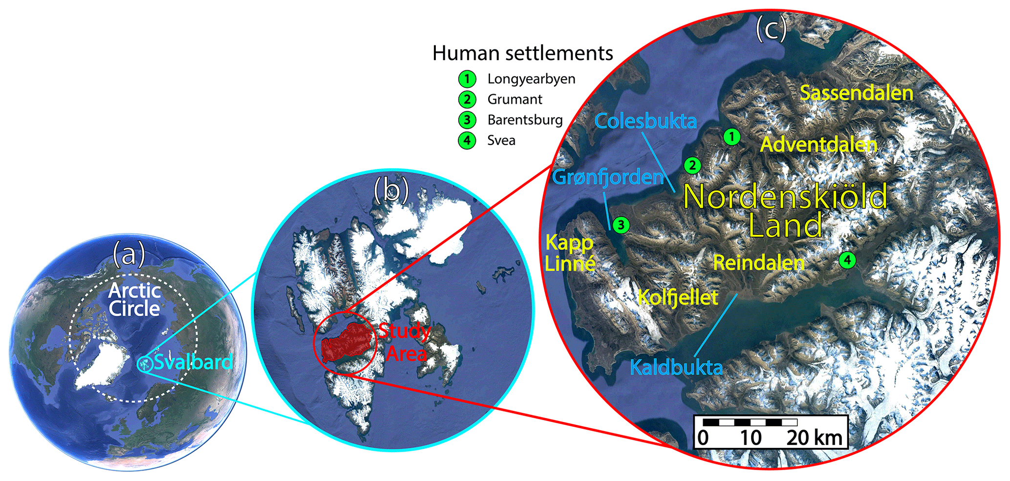
Figure 1 Panels showing location of the study area in the context of (a) the Northern Hemisphere, (b) the Svalbard Archipelago, and (c) local settlements, with colour-coded details where toponyms appear in yellow and fjords in blue (base maps from © Google Earth).

Svalbard represents one of the most diverse geological landscapes in the world, where sections representing most of the Earth's history are accessible. Outcropping bedrock formations in Svalbard range from the Archaean to Quaternary in age and were uplifted during the Cenozoic era (Koevoets et al., 2019). Geologically, the peninsula is part of the contact zone of two large structures of the first order: the horst-anticlinorium of the western coast of Spitsbergen and the West Spitsbergen graben. Quaternary deposits (soft sediment) consist of isostatically raised marine sediments in the lowlands, glacial and glacio-fluvial deposits in the valleys, extensive and complex slope deposits, areas of aeolian sediment cover, and extensive in situ weathering of bedrock. The landscape is particularly diverse: from watershed peaks to the landscapes of U-shaped valleys, extensive mountain plateaus, small valley glaciers and moraines, and coastal plains. Much of the terrain hosts marked mountain surfaces, steep slopes, and moraines draped by primary and Arctic desert soils with thin herbaceous–moss–lichen groups. All sediments and bedrock are heavily influenced by the perennial frost in the ground (permafrost) (Demidov et al., 2021). Over time, especially the more fine-grained deposits have accumulated an excess of ground ice, especially the upper 1–5 m of the permanently frozen soil (Gilbert et al., 2018).

The Nordenskiöld Land area was specifically chosen for this study because it represents the largest and most compact ice-free peninsula of the Svalbard archipelago, located between Isfjorden, Van Mijenfjorden, and Bellsund (Fig. 1c). It also represents the area where most of the human settlements (Longyearbyen and recreational huts in the vicinity, Barentsburg, and Svea – a mining city whose activities may be decommissioned soon) and infrastructure are located. In addition, there is a lot of transport by snowmobile and dog sledding during the winter season and movement on foot in this area for recreational and practical purposes. This makes the present study highly relevant from a societal point of view, considering that this century the Arctic will undergo the most rapid projected climate change than any other region around the globe (Ford et al., 2021).

3 Methodological context and strategy

Hydro-morphological hazards at middle to low latitudes are regularly mapped, and their information is freely shared in local and global databases. This is the case for co-seismic (Schmitt et al., 2017; Tanyaş et al., 2017) and rainfall-induced (Kirschbaum et al., 2009; Emberson et al., 2022) landslides, and the same is also valid for floods (Adhikari et al., 2010). The part of the geoscientific community working on cryospheric hazards has not yet produced global products, but current trends have seen an increase in data sharing, with thaw slump inventories often becoming part of supplementary materials in recent publications (Ramage et al., 2017; Lewkowicz and Way, 2019; Swanson, 2021; Nitze et al., 2018). Our aim here is to align with this movement and share the latest version of our TS and TEG inventories mapped for the Nordenskiöld sector in Svalbard. In Sect. 3.1, we provide a detailed description of the two inventories.

Moreover, another aspect differentiates research carried out at middle to low latitudes with respect to the trends in the Arctic context. In fact, hazard inventories have been commonly used for susceptibility modelling since the early years of 1970 (Brabb et al., 1972), and their results are presented as having both explanatory (Lombardo and Mai, 2018) and predictive (Lima et al., 2021) purposes. The explanatory element of these models is usually meant to interpret why they occur where they occur based on statistical relations between the locations where these hazards take place and their landscape and environmental characteristics (Steger et al., 2021). As for the predictive aspect of these models, they are used to probabilistically define areas where these processes may currently be absent, but their characteristics imply that they could manifest in the future (Reichenbach et al., 2018). As a result, decision-makers can plan suitable remedial actions, if needed, or assign land use development constraints (Roccati et al., 2021). High-Arctic environments have not received the same modelling attention with few exceptions (e.g. Blais-Stevens et al., 2015; Luoto and Hjort, 2005) despite their inarguably unique and pristine vulnerable landscapes threatened by global warming. Therefore, our intent is to expand the available literature on data-driven models applied to cryospheric hazards and demonstrate their potential as tools to understand local dynamics, as well as predict locations that will undergo the same surface deformation process.

3.1 Cryospheric hazard inventory

To build a comprehensive inventory of the two cryospheric hazards (TSs and TEGs), the most recent orthophotos (5×5 m pixel size) acquired in 2009–2011 from the Web Map Services (WMS) of the Norwegian Polar Institute (NPI, 2022a) were interpreted. Unfortunately, no subsequent imagery has been collected in the last 10 years, and the available scenes in Google Earth and Esri Wayback Imagery are quite coarse and unsuitable for detailed mapping of the relevant features. Most of both TSs and TEGs appear to be fresh or partly active landforms and can thus be considered recent. TSs (Fig. 2a) and TEGs (Fig. 2d) were morphologically identified, digitised on-screen as polygons, then quality checked in the GIS environment. Notably, this operation was repeated twice by two separate Arctic geomorphologists who acted independently. The resulting inventories were then examined and combined into a final digital version. To further validate the mapping, a series of field campaigns were organised and distributed over 3 years (2020–2022). On each occasion, two scientists went to the field, visited several representative sites, and judged the mapping results. During these visits, aerial surveys were also undertaken using unmanned aerial vehicles (UAVs), whose example images are shown in Fig. 2b and c. In addition to those, direct photos were also collected (see Fig. 2e and f). To complement the field surveys, we also brought a Trimble S5 series motorised total station and a Trimble TSC3 controller for long-term monitoring, whose use was limited to a few specific TEG locations.

Aside from manual mapping examples, it is important to stress here that the use of deep learning architectures has recently started to produce interesting results for automated cryospheric hazard mapping, with viable examples both for TSs (Xia et al., 2022; Huang et al., 2020, 2022) and TEGs (Huang et al., 2017). However, their implementation has not matured yet into operational mapping tools, and for this reason, we have opted to manually interpret and digitise the two inventories with the aim of producing them with the highest quality and completeness.

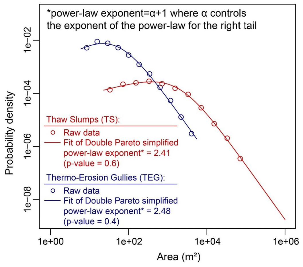
We examined the frequency–area distributions of both TS and TEG inventories based on approaches widely used in the landslide literature (Malamud et al., 2004; Tanyaş et al., 2018). A few studies show that a power law exists for medium and large landslides, and the slope of the power law (power-law exponent) is used to explore a link between the power-law exponent and regional differences in structural geology, morphology, hydrology, and climate (Densmore et al., 1998; Li et al., 2011; Hergarten, 2012). However, these kinds of analyses are not common for TSs or TEGs in general. In fact, even the validity of power law has not been examined in detail yet. Given this motivation, we analysed frequency–area distribution curves of the inventories and assigned a fit to each using double Pareto simplified function (Rossi et al., 2012). We also checked the validity of power-law fitting using the Kolmogorov–Smirnov (KS) statistic that generates a p value indicating the plausibility of the hypothesis (Clauset et al., 2009). A p value close to 1 indicates a good fit to the power-law distribution, whereas a p value equal to or less than 0.1 might indicate that the power law is not a plausible fit to the data.

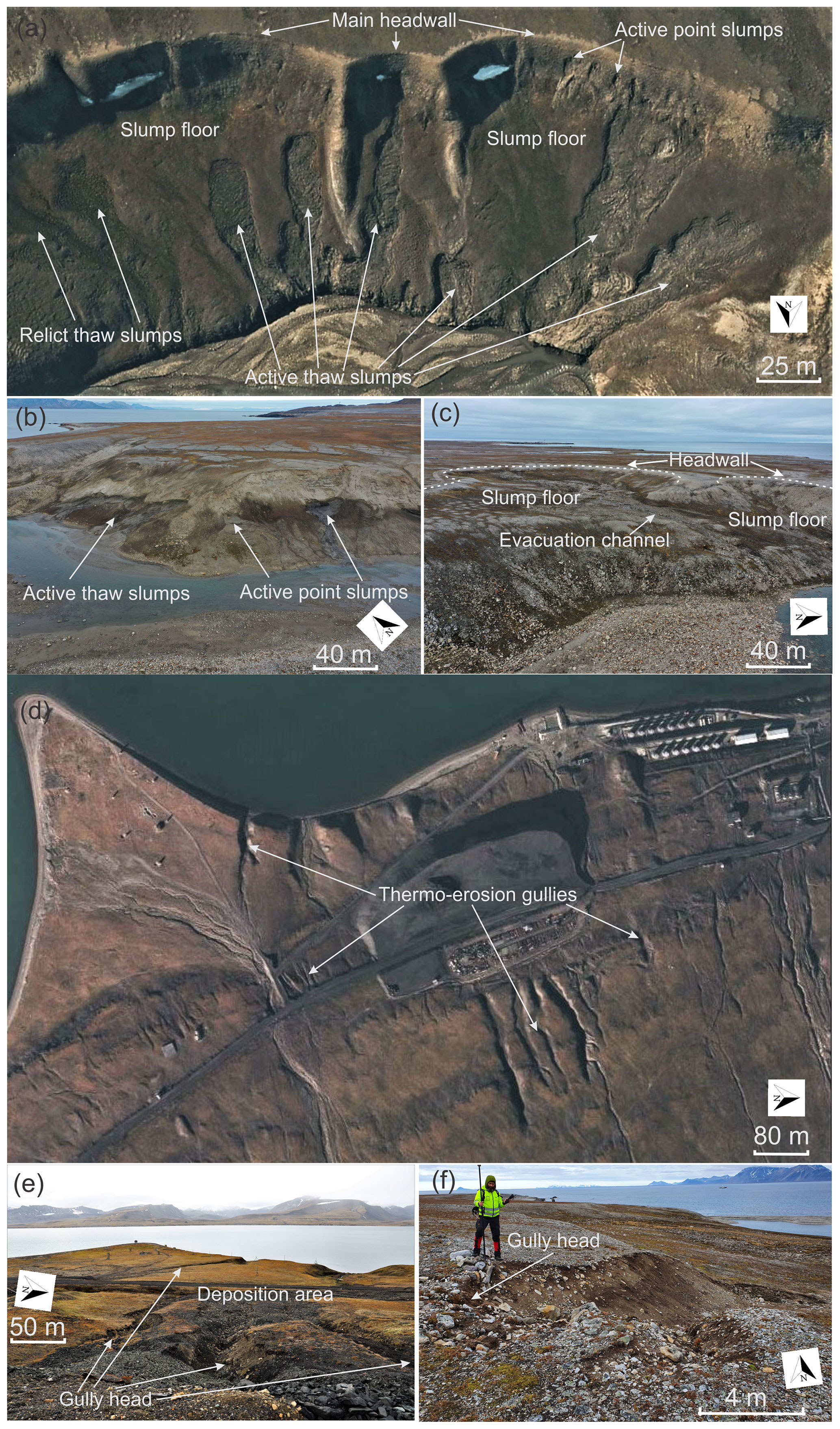
Figure 2 (a) TSs on a north-facing slope on the left side of the Hanaskogelva river in proximity to Advent City (orthophoto by © NPI, 2022a). (b) UAV photo of active TSs and active point slumps along the right side of Linnéelva river, close to Russekeila. (c) UAV photo of an inactive TS (left side) and an active TS (right side) along the left side of Linnéelva river, close to Russekeila. (d) Thermo-erosion gullies on a western-facing slope in Finneset, south of Barentsburg (orthophoto by © NPI, 2022a). (e) Photo of gully heads and their deposition areas south of Barentsburg. (f) Gully head cut into uplifted beach and marine deposits on the left side of Linnéelva river, close to Russekeila.

3.2 Environmental variables for statistical analysis

Due to the terrain settings of Nordenskiöld, as well as known morphological and geological attributes associated with thermokarst activity and specifically to TSs and TEGs, we selected several environmental variables (Ward Jones et al., 2019; Lacelle et al., 2010), which are presented in Table 1.

Table 1 Environmental variables used in the study.

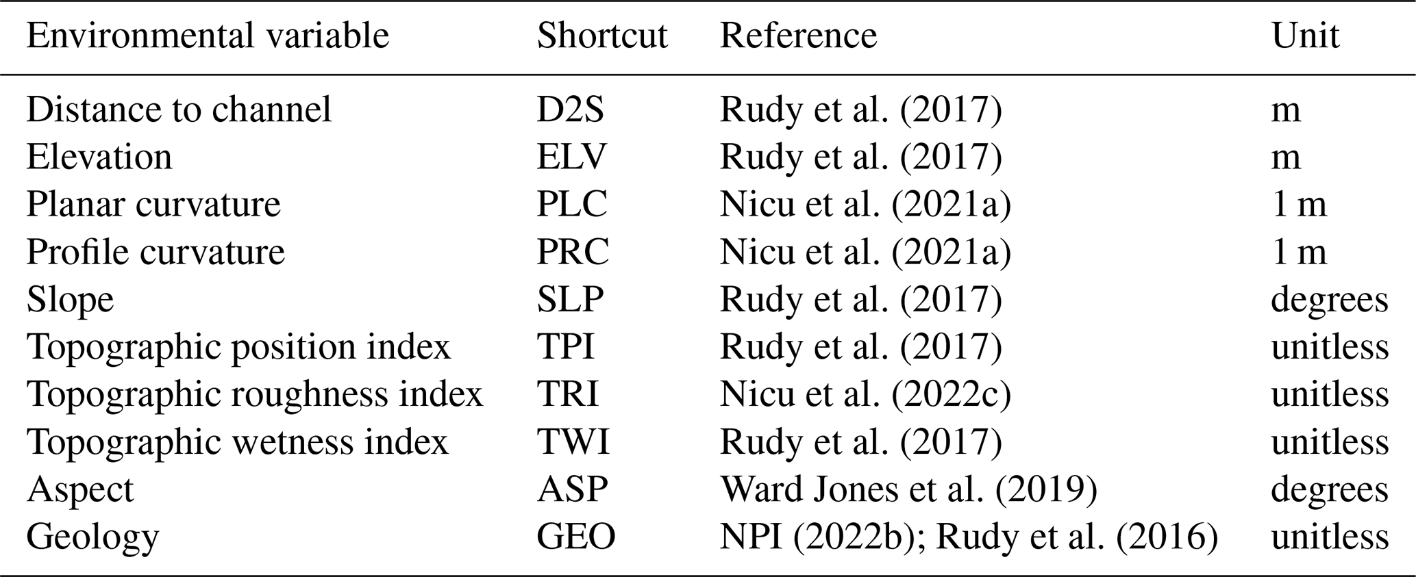
Out of these covariates, the terrain ones originated from a 5 m DEM (Melvær et al., 2014). However, keeping this resolution would have led to 122×10⁶ grid cells for the whole study area, and therefore, we opted to upscale the grid resolution to 100 m for computational reasons. Also, the Norwegian regulations require that cultural heritage sites should be marked as at risk if closer than 100 m from the nearest cryospheric hazard. Therefore, a grid cell size of 100 m ensured a reasonable computational burden for the analyses to be carried out later, and it also represented a meaningful mapping unit for disaster risk reduction practices. Such an operation resulted in partitioning Nordenskiöld Land into ∼300 000 grid cells. These have been assigned with the value of the corresponding covariate by taking the mean value of 5 m. As for the ASP (aspect), we reclassified it into 16 classes, each one 22.5^∘ apart. Then, also for the GEO (geology), we assigned the 100 m grid cell the predominant categorical class.

3.3 Model training and validation

Our modelling strategy relies on a generalised additive model (Titti et al., 2021). This class of models ensures the same level of interpretability as the simpler and more common generalised additive model (Atkinson et al., 1998; Titti et al., 2022) while providing much higher performance which is close to more complex architectures belonging to machine/deep learning (Aguilera et al., 2022). A GAM can be used to explain data distributed in a few exponential family distributions (gamma, Gaussian, etc.). Among these, the ideal framework to model dichotomous data corresponds to the binomial case, in which in the context of our work, TSs and TEGs are separately assumed to occur spatially according to a Bernoulli distribution (Bryce et al., 2022). A binomial GAM can be denoted as follows:

$$\mathit{\eta }\left(\mathit{\pi }\right)=\log \left({\displaystyle \frac{\mathit{\pi }}{\left(\mathrm{1}-\mathit{\pi }\right)}}\right)={\mathit{\beta }}_{\mathrm{0}}+f_{\mathrm{1}}{x}_{\mathrm{1}}+f_{\mathrm{2}}{x}_{\mathrm{2}}+\mathrm{\dots }+f_{\mathrm{n}}{x}_n,$$

where η is the logit function, π is the probability that the response is present at a given location, β₀ is the global intercept and f_n is the nonlinear function estimated for each covariate in the model. In traditional regression problems, the input is a continuous quantity, and the output is the same. In our case, the input data for the response variable consist of a vector of zeroes and ones, standing for absence and presence locations. Conversely, the output is expressed in a continuous spectrum of values that represent the probability of occurrence of our response. Therefore, a series of metrics have been developed over time to express the performance of the binary classifiers. All of these can be clustered into cut-off dependent and independent metrics, where the former boils down to the selection of a specific value to reclassify the probability spectrum into a binary dataset, from which confusion matrices can be computed (Bertolini, 2021). The latter type relies instead on many probability thresholds to compute true positives and negatives, as well as false positives and negatives, from which metrics such as receiver operating characteristic (ROC) and their area under the curve (AUC) can be computed (Hajian-Tilaki, 2013).

Aside from the context provided above, a distinction must be made between binary classifications oriented toward explanatory and predictive assessments. The former interprets the functional relations estimated multi-variately by regressing the vector of presence/absence with respect to the covariate set. This can usually be done based on the full available information. For instance, in our work, this implies using 100 % of the grid cells of our study area. However, the estimated results cannot be interpreted for prediction, and this is achieved via two common approaches. If temporal data are available, then the prediction skill of a given classifier can be measured by matching the susceptibility estimated from a given time over the presence/absence distribution of the subsequent period. However, this is a rarely performed task because multi-temporal hazard inventories are still not common (Guzzetti et al., 2012). This is even more valid in peri-Arctic environments, where hazard inventories are scarce even in their pure spatial form. Therefore, when the data dimension is spatially confined, a well-established routine to estimate predictive performance relies on splitting the spatial data into a portion used for calibration and another one for validation under the assumption that spatial replicates mimic the behaviour of temporal ones. The training and test split though can also be done in diverse ways. The simplest corresponds to pure random cross-validation (RCV; Roberts et al., 2017), although such a practice usually leaves the data structure like the original set, therefore also returning similar performances to the calibration ones. A complementary validation routine uses a spatially constrained subset of the data instead. This is usually referred to as spatial cross-validation (SCV; Brenning, 2012) and offers the ability to assess sectors of a given study area for which the model may locally perform well or fail.

In this work, we make use of all the elements described above: we fit the presence/absence data to the whole Nordenskiöld landscape, and we use the results for interpretation. As for assessing the predictive skill, we also perform the two cross-validations (a 10-fold RCV and an 8-fold SCV) for both TSs and TEGs.

4 Results and discussion

The resulting inventories encompass 562 TSs and 908 TEGs. Compared to the previous preliminary study (Nicu et al., 2021a), the RTS inventory has increased from 400 to 562 polygons. As for the TEGs, the updated version of our inventory included 908 polygons, 98 more than were mapped in a previous study (Nicu et al., 2022c). This final effort brought our inventories to their current and final form, in which the mapping procedure covered the whole study area shown in Fig. 1, and field surveys have validated some of their positions and extent.

The inventories are of high value in a climate change context, as they can be of use to a wide range of scientists, such as geomorphologists, climatologists, hydrologists, biologists, and archaeologists, as well as stakeholders and local authorities, in their effort to quantify the potential impacts of the two hazards on infrastructure (Hjort et al., 2018, 2022) and cultural heritage (Nicu et al., 2021a, 2022c). To explore their characteristics for any of the users and uses mentioned above, below we will summarise the frequency area distributions (FADs) of the two inventories we mapped, and in the subsequent sections, we will present the results of the susceptibility modelling we performed.

4.1 TS and TEG size characteristics

First, we checked the validity of the power law for the generated dataset. Based on the KS test, we calculated p values, which are larger than 0.1 for both TS (p value =0.6) and TEG (p value =0.4) inventories. This shows that for both inventories, a double Pareto simplified function is a numerically plausible fit to the data (Fig. 3). Second, we identified power-law exponents. Power-law exponents simply show the ratio between small and medium/large landslides. In our case, we calculated them as 2.41 and 2.48 for TSs and TEGs, respectively. Interestingly, these values were a perfect match with observations carried out for landslides triggered by an earthquake, rainfall, and snowmelt where the average power-law exponent centralised around 2.4 (e.g. Malamud et al., 2004; Tanyas et al., 2018). Among numerous factors controlling the power-law exponent of landslide inventories, the topography is one of the most mentioned parameters in the literature (Ten Brink et al., 2009). Here, our results show a clear match between power-law exponents of landslides and TSs/TEGs, although TSs and TEGs are not generated along steep hillslopes as landslides are. Examining the reason behind this similarity is beyond the scope of this contribution. However, our results indicate that more TS and TEG inventories need to be generated to better understand their size statistics and factors governing the shape of their frequency–area distributions.

Figure 3 The FAD obtained for the two inventories in Nordenskiöld Land.

4.2 Susceptibility modelling performance

We measured both the goodness-of-fit and predictive skills of our modelling framework. Figure 4 reports the corresponding ROC and AUC values for the reference fitting procedure, as well as the two cross-validations. For both cryospheric hazards, the performance falls within the excellent category according to the AUC classification proposed by Hosmer and Lemeshow (2000). At a closer look though, the fit and RCV almost fall within the outstanding class (all the means are above 0.8 and below 0.9). The performance loss exhibited for the SCV is to be expected, and it represents an important indication. In fact, it highlights the prediction skill of our model assuming it to be blind to the characteristics of specific portions of the study area. Therefore, spatial cross-validation can be interpreted as the worst situation one can examine to understand a model prediction. Another element worth stressing is that the variability for the RCV is clearly low since a random selection is not able to disentangle local spatial dependence in the data. As for the SCV, where the spatial dependence is perturbed due to the constrained local selection, the variability is still within an acceptable range.

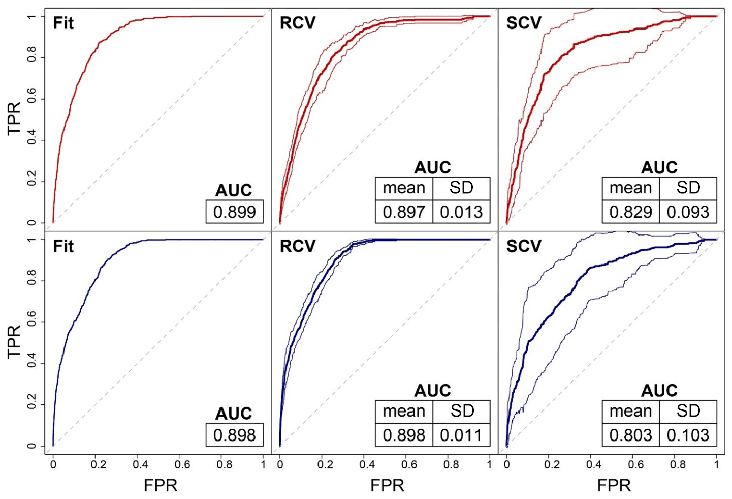
Figure 4 Modelling performance overview. First row indicates the results for TSs, whereas the second row reports the TEGs. The thick lines for the two cross-validation schemes represent the mean ROC curve, whereas the thin lines graphically summarise the variability in the cross-validation scheme via a single standard deviation.

4.3 Controlling factors of TSs and TEGs

From the original list of covariates shown in Table 1, we removed TRI and TPI because of a variable selection procedure. Specifically, their inclusion was slightly lowering the model performance and inflating the uncertainty in the other nonlinear covariate effects for both TSs and TEGs. At a closer look, we noticed that TRI was linearly related to SLP with a Pearson's correlation coefficient (ρ) above 0.9, whereas TPI showed a close dependence with respect to PLC attested by a ρ∼0.8. Figures 5 and 6 provide an overview of the selected covariate effects we used to model TSs and TEGs, respectively. The most striking element of the two figures is that the two processes we modelled share some similarities in the way some of the covariates are influencing their occurrence, although some marked differences also exist. For instance, both TSs and TEGs occupy the lowlands of the Nordenskiöld landscape, being the ELV contribution dominant within the first 200 m above sea level, after which the effect rapidly decays and becomes heavily negative after a height of approximately 300 m. From a first glance, this indicates a positive relation of both processes to sorted and fine-grained sediments, which are found as isostatically uplifted marine and glaciomarine sediments along the coasts and as fine-grained valley fills of fluvial and aeolian origin in the rest of the landscape of lower elevations. Conversely, it speaks against a connection to the often-extensive sediment covers of in situ weathering material on the higher mountain plateaus. This initial consideration about TS and TEG co-existence is enriched when considering other covariates' effects.

Differences start to arise when examining the D2S, which strongly contributes to TSs' occurrences within tens of metres and drastically drops after that, up to negative effects after a few hundred metres away from the channel. This effect may have to do with riverbank erosion at the base of a potentially unstable permafrost slab, which once it misses its support starts moving and further develops into a retrogressive slump. It might also be secondarily linked to some snow-bank effects on the initiation of a TS, where thermal conductivity through percolating meltwater from the snow during summer seasons might be of importance. The arctic winters with often high wind speed favours the intensive redistribution of snow over the landscape, accumulating in low positions like, for example, channels. Interestingly, this is not the same effect shown for the TEG case where the contribution to the susceptibility is shown to increase 500 m away from a streamline. This may be because to form a gully needs an incision to develop. A streamline represents an incision that has already widened in time, and therefore, it is only reasonable for TEGs to manifest a bit further away.

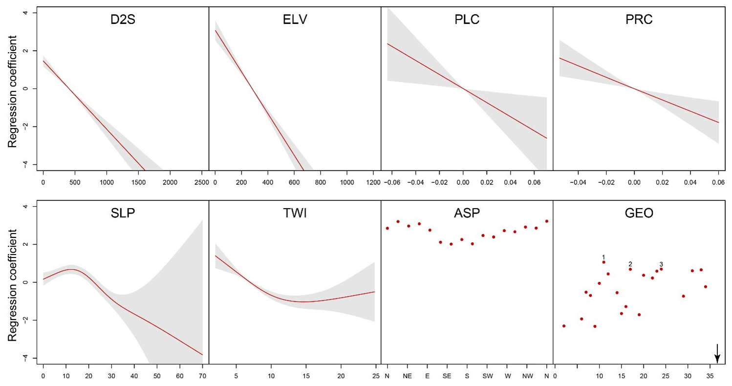
Figure 5 Covariate effects estimated for TSs. Notably, the regression coefficients estimated for outcropping lithologies also host strong negative values. For pure visualisation purposes, we have focused on representing a coefficient range in which the positive classes would still appear to be visible. Also, to avoid clustering the text, we have described in the text only the three strongest and positive contributors, labelled 1, 2, and 3 in the image.

The image of the landscape prone to the two processes can be further diversified by looking at SLP, where both processes show quite different behaviour. The probabilistic occurrence of TS is favoured up to 20^∘, after which the SLP contribution becomes increasingly negative. As for TEGs, the overall SLP contribution appears negligible, with the first tenths of degrees being slightly positive and the remaining steepness domain becoming slightly negative. This indicates once more that TSs do form in near-flat areas, whereas TEGs can also occur along steeper morphologies. There, the overland and/or interstitial flows would accelerate over preferential directions giving rise to linear erosion forms that may further develop into gullies. As for the exposition, some degree of similarity can be seen once more, with the north, north-east, and north-west directions contributing to an increase in the probability of TS and TEG occurrence.

The geological control is extremely complex and would require listing tens of lithotypes; however, this is not the primary focus of this paper. Firstly, we can conclude from the field and remote sensing data that most, if not all, of both TS and TEG occurrences are situated in soft sediments (Quaternary deposits). This is not surprising, given that they both rely on grain-to-grain conditions with and without permafrost internal ice. Since Nordenskiöld Land lacks continuous data on Quaternary geological sediment, this is not included in the statistical analysis. Knowledge of the connection between bedrock and deposition of sediments indicates that local bedrock is however often linked to the soft sediment deposits. This assumption is especially true for in situ weathering slope deposits, fluvial deposits, and glacial tills but a little less obvious for marine deposits. This relation prompted us to look at bedrock lithology (where regional data are available) as one factor in the analysis.

For reasons of conciseness, we opted to report the three highest contributors with a positive sign to express lithotype characteristics prone to host TSs and TEGs. Specifically, the probability of TSs appears to increase in areas overlying bedrock of shales (bituminous), siltstones, and sandstone mixed deposits dated back to the Late Jurassic–Early Barremian. This is again the case for bituminous shales and siltstone mixed deposits that originated during the Late Jurassic. The third lithotype prone to TSs is also the highest contributor to TEGs, this consisting of shales, mudstones, and siltstones of the late Palaeocene. The second highest geological contributor for TEGs consists of a mixture of sandstones, shales, and coal formed again during the Palaeocene, and the third one is represented by a deposit hosting sandstones and conglomerates of the Barremian. This is clearly an interesting description of the geological effects because the model out of many different classes consistently picked the same lithotypes as predisposing factors for TSs and TEGs, with minor differences represented by coal and conglomerate inclusions.

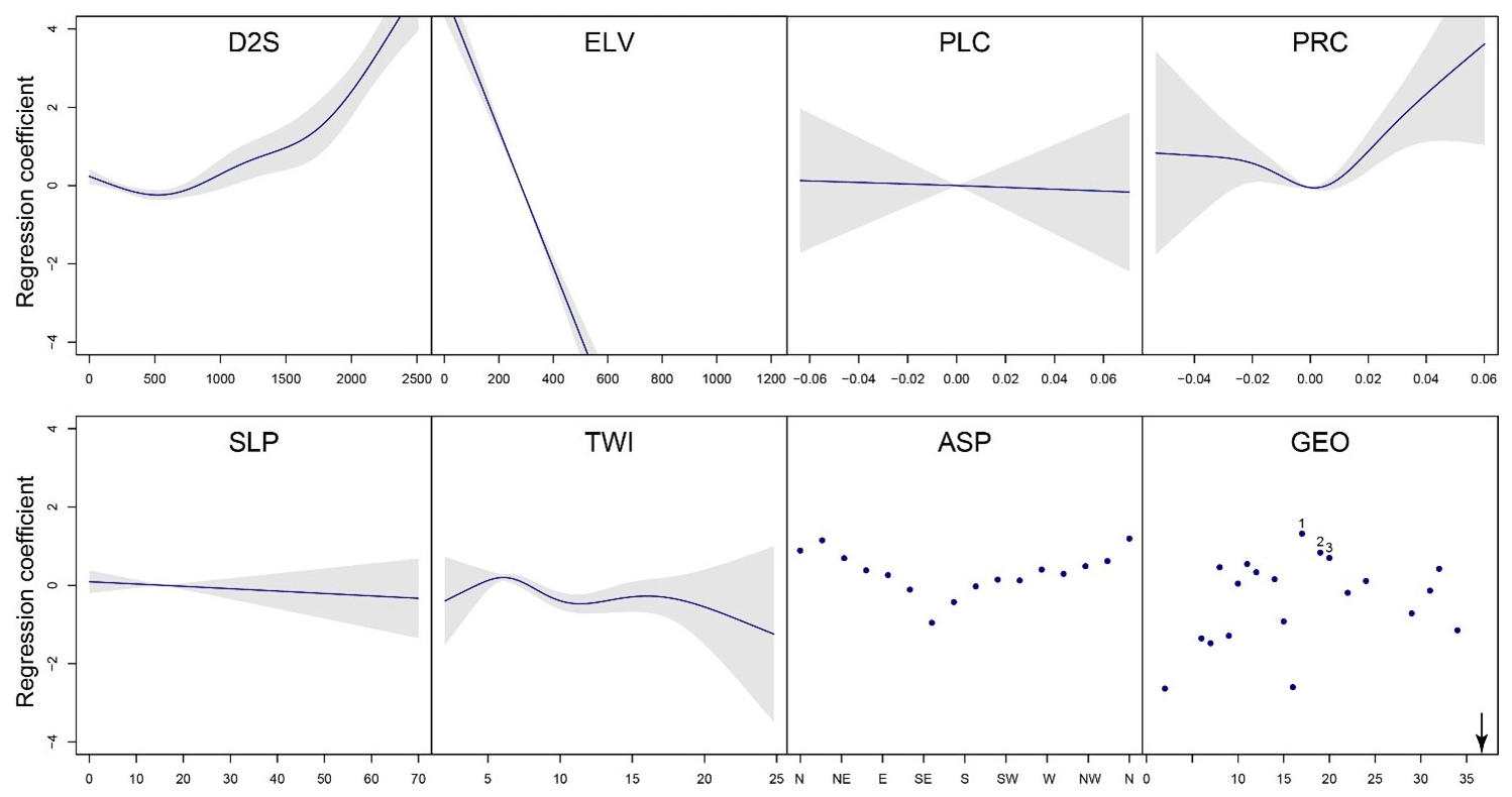
Figure 6 Covariate effects estimated for TEGs. Notably, the regression coefficients estimated for outcropping lithologies also host strong negative values. For pure visualisation purposes, we have focused on representing a coefficient range in which the positive classes would still appear to be visible. Also, to avoid cluttering the text, we have described in the text only the three strongest and positive contributors, labelled 1, 2, and 3 in the image.

4.4 Susceptibility mapping of TSs and TEGs

The satisfactory performance and the reasonable effects presented above suggest that the models we produced for TSs and TEGs are reliable and can be considered for susceptibility mapping. To graphically summarise this task, we produced two overviews, one where the susceptibility values are shown in their continuous form and one where we grouped them into classes. Figure 7 shows these two options both for TSs and TEGs.

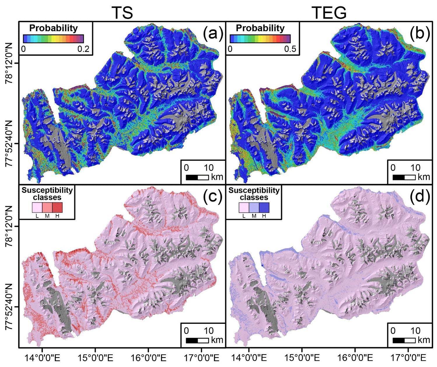
Figure 7 Susceptibility map reporting the probability in its continuous (a, b) and classified (c, d) forms for TSs (a, c) and TEGs (b, d), respectively. Grey areas correspond to glaciers which have been masked out from the analyses. The classification followed the Jenks method by minimising the within-class variance after an arbitrary choice of three classes (L for low, M for medium, and H for high susceptibility).

The TS susceptibility patterns (left column) appear to be distributed along the coastlines and in part of the central-western sector of Nordenskiöld Land, supporting the link to the raised marine deposits. Specifically, coastal areas likely to host new formations of TSs can be found between Heerodden and Eriksonodden (Colesbukta), Festningsodden and Kokerineset (western part of Grønfjorden), scattered areas between Kapp Linné and Kapp Starostin, Vestpynten and Adventpynten (close to Longyearbyen Airport), and in the northern part between Diabasodden and Elveneset and Vindodden. The reason these locations are relevant for the Nordenskiöld community is that they are also locations where or close to where most human activities take place on the island. As for areas susceptible to TEGs (right column), these are characterised by a higher probability of occurrence while also being more concentrated in a few areas. These areas overlap with main human settlements (Longyearbyen and Barentsburg) and former mining settlements (Grumant and Svea) to the point that it raises the question of whether the formation of TEGs may be partially due to anthropic effects. Other than being speculation though, no obvious signs of such spatial dependence were found during our fieldwork activities, and thus it is an observation we opted to share with the readers but also to reject from our own experience.

It is worth mentioning that the difference in probability range shown for the two cryospheric hazards is also because TEGs are more numerous than TSs; thus the different proportion of the presence/absence data influences the global intercept, making it less negative for the TEGs than for the TSs. However, this effect still allows for the spatial predictive patterns to be suitably depicted, with differences that emerge based on the landscape characteristics. Nevertheless, these patterns are still portrayed in a separate manner, therefore making it difficult to perceive areas where they clearly co-exist. In the next section, we will address this issue by providing details on how we generated a map capable of showing the probabilistic assessment of multi-cryospheric hazard occurrences for Nordenskiöld Land.

4.5 Multi-cryospheric hazard susceptibility mapping

To simultaneously represent the likelihood of TSs and TEGs within the same map, we opted to combine the two reclassified maps previously shown in Fig. 7. The resulting multi-hazard susceptibility map is shown in Fig. 8, where nine classes are portrayed through a two-dimensional colour bar, reflecting the RGB (red–green–blue) combination of the three classes per hazard in Fig. 7. Most of Nordenskiöld falls in the LL category, and the extent of the other eight classes exponentially decreases as the combined susceptibility level increases. However, the site being extremely large, this still implies that some portions of the territory may be subjected to either or both cryospheric hazards. For this reason, we also report the total extent of the nine classes (whose graphical expression is plotted as a bar plot within Fig. 8), with LL covering 2657 km², LM 244 km², LH 4 km², ML 37 km², HL 0.48 km², MM 112 km², MH 20 km², HM 0.04 km², and HH 0.03 km².

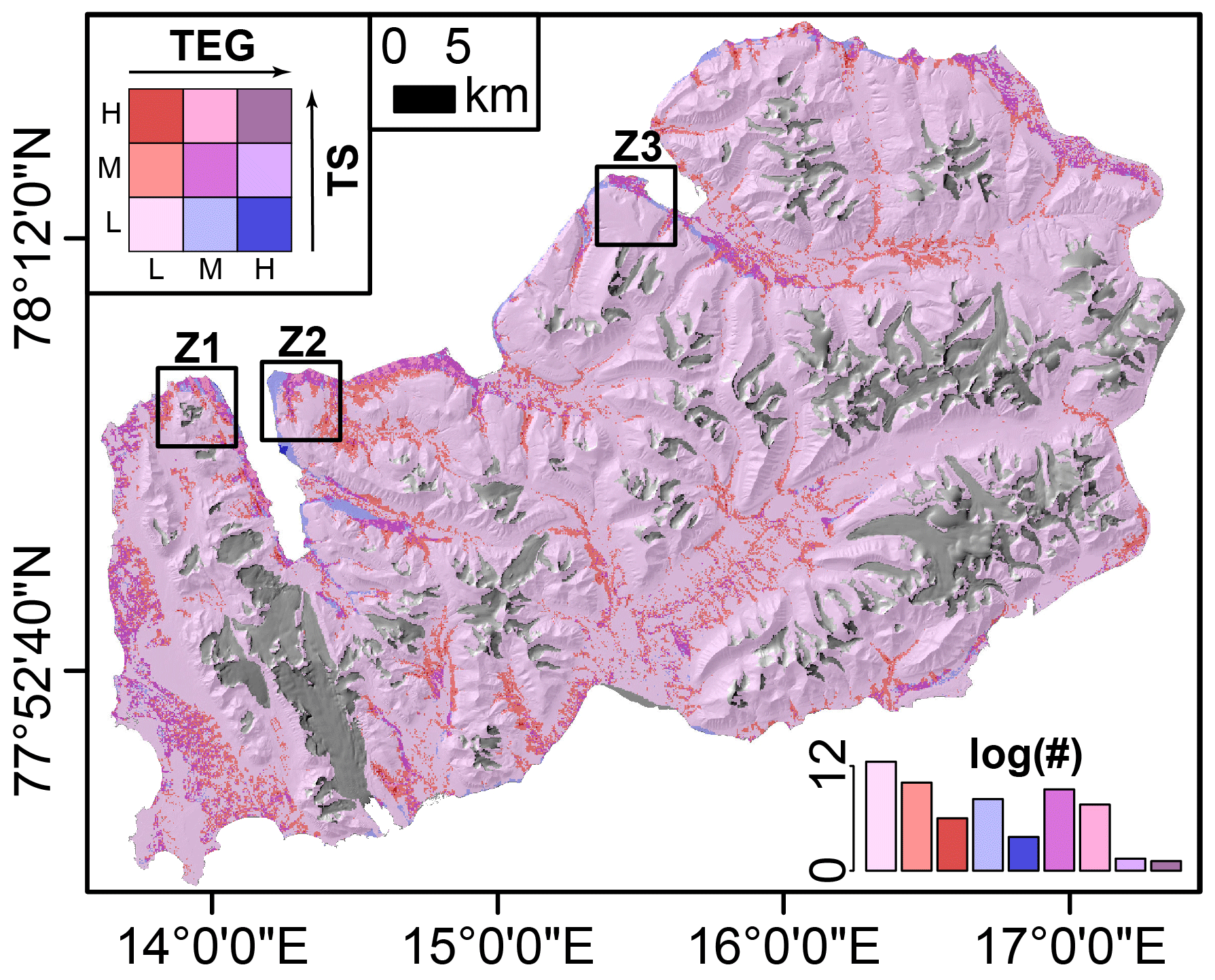
Figure 8 Multi-hazard susceptibility map of TSs and TEGs for Nordenskiöld Land. The bar plot at the bottom right represents the number of grid cells expressed in logarithmic scale for each of the nine combined susceptibility classes.

The most susceptible areas to both cryospheric hazards are located along the coastlines from the central, north-western, south-western, and north-eastern parts of Nordenskiöld Land. Three suggestive examples are shown in Fig. 9 to highlight details of the multi-hazard estimates. These are locations of actual relevance for Nordenskiöld Land, as it contains human settlements that are prone to danger, especially its infrastructure. Z1 shows the area prone to Stemmevatnet lake, which represents the main water resource for Barentsburg. Any future TS and/or TEG processes may jeopardise this aspect. Z2 highlights the area around and north of Barentsburg, where important infrastructure and protected cultural heritage are located. Finally, Z3 shows the main settlement, Longyearbyen, along with the area around the airport. This is of high importance for local authorities and stakeholders in their effort to minimise future disturbance of the local infrastructure and protected cultural heritage sites.

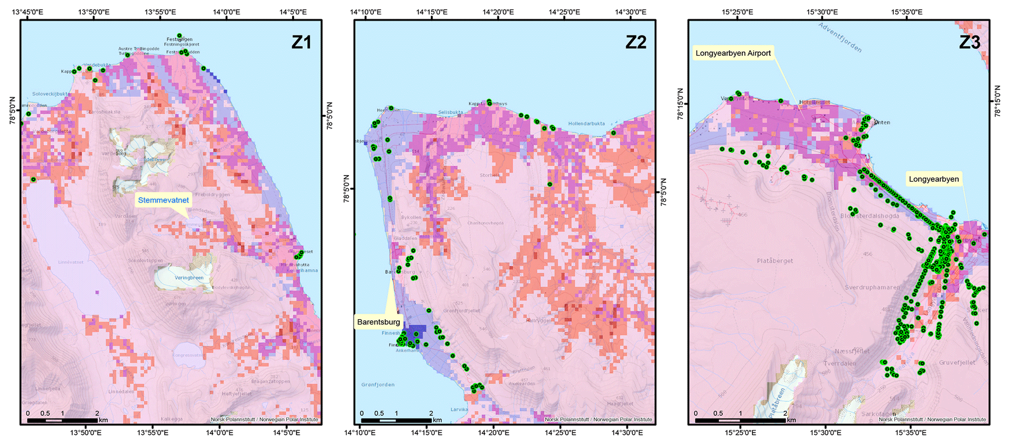
Figure 9 Multi-hazard map overlaps with zooms 1, 2, and 3 highlight portions of the territory where the two cryospheric hazards can interact with human activities, local infrastructure (in red and black lines), and protected cultural heritage (green points).

5 Considerations within and beyond Svalbard: supporting and opposing arguments

A systematic TS and TEG mapping protocol to share these cryospheric hazards among researchers has yet to root within the geoscientific community. This work aligns well with other attempts to make data on TSs and TEGs freely accessible because we believe that the surface deformation dynamics of delicate environments laying within Arctic and peri-Arctic regions can be studied only as a collective effort. For this reason, we share our inventories in the hope of triggering similar behaviours within our community and stimulating the implementation of advanced models, as per other mid-latitude hydro-morphological processes.

Notably, until the use of automated mapping tools will become viable for cryospheric hazards, any manual mapping procedure such as the one we undertook here may suffer from subjectivity. To minimise any individual expert-based opinion and therefore remove its bias, in this work we implemented a collective mapping protocol in which two Arctic geomorphologists independently created the inventories only to be merged at a later stage. We believe this to be another requirement to be added to the collective effort we mention and recommend above. In fact, other studies have shown that collective mapping contributes to reducing uncertainties, which would otherwise become part of the data and propagate in any model one may build with it (Ardizzone et al., 2002).

Aside from the importance of a standard data-sharing platform within the global system, even just within the Svalbard context, this is something of great relevance. In fact, the study site we chose had undergone significant changes in recent times. The work of Ziaja (2001) has shown the extent of these changes in the form of permafrost degradation, whose dynamics can be better understood if framed within the bigger picture of the Svalbard meteorological settings.

In fact, Nordenskiöld Land has always been covered with a lesser glacier extent compared to the rest of the archipelago. This is due to the direction the maritime air masses follow in the area. Specifically, the effect of the warm West Spitsbergen Sea Current creates a convergence of mild and humid air from the south and chilly air from the north. This convergence results in a local micro-climate warmer than the rest of Svalbard and in general than what is typical at these latitudes. In addition to an already delicate situation, Ziaja (2001) observed that the deglaciation in Nordenskiöld Land has evolved at double the rate compared to Sørkapp Land (south Svalbard), arguing this to be an indication of a greater sensitivity of our study site to global warming. Therefore, we consider it vital to document and share evidence of permafrost degradation (our TS and TEG inventories) to reconstruct a baseline to which future monitoring protocols should refer for further exploring the effects of climate change in the area. One of the possible tools to use to explore these effects falls in the category of data-driven models, to which susceptibility studies belong. However, hardly any susceptibility studies have been carried out so far to estimate locations prone to TSs and TEGs in peri-Arctic regions (Blais-Stevens et al., 2015; Rudy et al., 2016; Veh, 2015).

Along this line of research, we proposed a tool for interpretable and flexible predictive models, offering the chance to explore the results from multiple aspects, among which we include a multi-hazard susceptibility assessment. The performance produced falls within the excellent class proposed by Hosmer and Lemeshow (2000). Therefore, standard practices would consider that such a model results in a piece of reliable information for local administrators to base their decisions on and plan a suitable course of action to reduce the risk due to these cryospheric hazards. This is already an important achievement; however, below we would like to stress a few elements that we already envision requiring further considerations to develop our model into an operational tool. Both TS and TEG processes are shown to be highly dependent on soft sediment characteristics, data which are so far lacking on Svalbard. Adding map data with the type and potential thickness of surface sediments would further increase the accuracy and detail of predictions. The other prominent issue we faced had to do with the absent temporal information in our inventory. This is something that unfortunately affects virtually all the TS and TEG inventories mapped across the globe. For this reason, we are limited to statically investigating and understanding locations prone to these hazards. However, this also raises the question of whether such information can be really used outside the academic context. In fact, any model without a temporal connotation will inevitably learn to mimic the process that occurred at the time of the orthophoto or satellite image used for mapping. In other words, no temporal information on temperature, rainfall, or other dynamic characteristics can be included in the model. Therefore, in a rapidly changing environment such as the Svalbard landscape, the probabilities of occurrences we estimated may have already been affected by global warming and permafrost degradation processes (Ziaja, 2004). With this in mind, we consider our workflow just a proof-of-concept of what can be achieved in the hope that in the years to come a broader scientific effort can bring together a fully spatio-temporal description of these cryospheric hazards. If this wish would become a reality, then a whole spectrum of different models and research questions will open for the geoscientific community to address. For instance, future simulations of TS and TEG probabilities at varying climate scenarios could be achieved by introducing, for instance, the temperature as a covariate and then using a plug-in simulation (Do et al., 2005; Lombardo and Tanyas, 2020) tool to project the change in susceptibility as the future temperature pattern changes. Fortunately, the status of the scientific branch focused on developing automated mapping tools has reached such a level of maturity that it is close to becoming widely adopted even in peri-glacial environments (Meena et al., 2022; Nava et al., 2022). For instance, the first article has already been published on the use of deep learning architectures for automated TS mapping (Huang et al., 2020). This represents a promising venue for multi-temporal mapping because each artificially intelligent mapper tool is run over a specific remotely sensed scene, and the same operation can therefore be repeated for each satellite orbit. Still remaining is the lack of spatially detailed and accurate data from the Arctic, where the processes discussed here required a ca. 5 m resolution for accurate detection of features to form a training dataset.

Another element that can be improved with future efforts has to do with the actual target of the model. So far, our aim was to estimate locations prone to TS and TEG formation. However, these processes also have a spatial extent, and the threat they may pose to local activities is equally if not more important than the simple notion of where they may initiate. For this reason, we already envision future models that would take the measured extent of TSs and TEGs as the response variable, this time solving a regression task rather than a classification one as per the susceptibility requirement. Such a direction has recently been explored for landslides occurring at lower latitudes (Lombardo et al., 2021; Moreno et al., 2022). An even better extension has already been tested in which the expectation of locations prone to landslides are modelled, together with the expectation of the resulting landslide size (Aguilera et al., 2022; Bryce et al., 2022).

Notably, all these methodological considerations are valid extensions to be tested within the Svalbard landscape. However, they can also be valid outside it. If space–time models do become a viable approach because multi-temporal inventories also become available, then dynamic simulations could also be extended to the whole peri-Arctic sector. This would enable large-scale considerations on climate change and its cascading influence from temperature to TS and TEG spatio-temporal patterns.

At a global level, permafrost is undergoing considerable degradation following the increasing trend of global warming. Recent studies highlighted the fact that the Arctic has warmed 4 times faster than the globe since 1979 (Rantanen et al., 2022). This leads to TS and TEG occurrences, which can pose a threat to Arctic infrastructure (Hjort et al., 2022) and cultural heritage (Nicu et al., 2021a, 2022c), impact the fluvial sediment budget (Lamoureux and Lafrenière, 2018), and release significant amounts of greenhouse gases, such as carbon dioxide and methane, to the atmosphere (Oberle et al., 2019; Ran et al., 2022). Cryospheric hazards are likely to further increase in the future following climate change (Ding et al., 2021), and using the latest statistical advances to predict their likely occurrences is of paramount importance. This study showed the importance of the two inventories and what can be achieved when using them both separately and together in a multi-hazard approach. The method can be adapted and transferred to the entire ice-free area of the Svalbard Archipelago and other circumpolar areas. The final multi-hazard map represents a valuable tool that can be further processed and improved for local authorities and policy makers (Nicu and Fatorić, 2023) and can be transformed into plans at various scales of mitigation and adaptation measures (Nicu, 2022).

6 Data availability

The NPI images are freely available at https://geodata.npolar.no/ (NPI, 2022a). The digital elevation model is freely available at https://doi.org/10.21334/npolar.2014.dce53a47 (Norwegian Polar Institute, 2014). The Geological Map of Svalbard (Geologi Svalbard), in raster format, scale 1:250 000, is freely available at https://geodata.npolar.no/arcgis/rest/services/Temadata/G_Geologi_Svalbard_Raster/MapServer (NPI, 2022b). The TS and TEG inventories are publicly available in shapefile format at https://doi.org/10.1594/PANGAEA.945348 (Nicu et al., 2022a) and https://doi.org/10.1594/PANGAEA.945395 (Nicu et al., 2022b), respectively.

7 Conclusions

At a global level, permafrost is undergoing considerable degradation following the increasing trend of global warming. Recent studies highlighted the fact that the Arctic has warmed 4 times faster than the globe since 1979. To better understand what the expectations of future permafrost degradation-related processes are, a systematic sharing practice of the mapping routines we perform as a community should become commonplace. In line with this objective, in this work, we share the TS and TEG inventories we mapped and validated through several field campaigns. Moreover, to better understand these processes and attempt to reliably predict them, the implementation of data-driven models holds promising potential. This is also the case for cryospheric hazards such as TSs and TEGs, whose occurrence probability we propose here to be modelled via a binomial GAM. We also take it a step further and produce a multi-hazard susceptibility map of our test site in Nordenskiöld Land. These types of models are also rare in peri-Arctic environments, and their spread may lay the foundations to build a global assessment of cryospheric hazards' development as a function of global warming. This is the direction we consider to be crucial for assessing the risk that Arctic communities may soon be exposed to. This is something of fundamental importance because the changes we have witnessed in the recent past and that we see today will be relatable to the changes we will see in other permafrost-rich areas such as the Alps or the Himalayan range. Their global warming has yet to reach the extent of the change we have observed so far near the pole and therefore in Svalbard.