the Creative Commons Attribution 4.0 License.
the Creative Commons Attribution 4.0 License.
 | 13 Sep 2023
Barium in seawater: dissolved distribution, relationship to silicon, and barite saturation state determined using machine learning
Adam V. Subhas
Heather H. Kim
Ann G. Dunlea
Laura M. Whitmore
Alan M. Shiller
Melissa Gilbert
William D. Leavitt
Tristan J. Horner
Barium is widely used as a proxy for dissolved silicon and particulate organic carbon fluxes in seawater. However, these proxy applications are limited by insufficient knowledge of the dissolved distribution of Ba ([Ba]). For example, there is significant spatial variability in the barium–silicon relationship, and ocean chemistry may influence sedimentary Ba preservation. To help address these issues, we developed 4095 models for predicting [Ba] using Gaussian process regression machine learning. These models were trained to predict [Ba] from standard oceanographic observations using GEOTRACES data from the Arctic, Atlantic, Pacific, and Southern oceans. Trained models were then validated by comparing predictions against withheld [Ba] data from the Indian Ocean. We find that a model trained using depth, temperature, and salinity, as well as dissolved dioxygen, phosphate, nitrate, and silicate, can accurately predict [Ba] in the Indian Ocean with a mean absolute percentage deviation of 6.0 %. We use this model to simulate [Ba] on a global basis using these same seven predictors in the World Ocean Atlas. The resulting [Ba] distribution constrains the Ba budget of the ocean to 122(±7) × 1012 mol and reveals oceanographically consistent variability in the barium–silicon relationship. We then calculate the saturation state of seawater with respect to barite. This calculation reveals systematic spatial and vertical variations in marine barite saturation and shows that the ocean below 1000 m is at equilibrium with respect to barite. We describe a number of possible applications for our model outputs, ranging from use in mechanistic biogeochemical models to paleoproxy calibration. Our approach demonstrates the utility of machine learning in accurately simulating the distributions of tracers in the sea and provides a framework that could be extended to other trace elements. Our model, the data used in training and validation, and global outputs are available in Horner and Mete (2023, https://doi.org/10.26008/1912/bco-dmo.885506.2).
- Article
(10294 KB) - Full-text XML
-
Supplement
(1979 KB) - BibTeX
- EndNote


Barium (Ba) is a Group II trace metal that is widely applied in studies of modern and ancient marine biogeochemistry despite lacking a recognized biochemical function (e.g., Horner and Crockford, 2021). These applications of Ba are based on two empirical correlations relating to its dissolved and particulate cycles. The first correlation relates to the dissolved concentration of Ba, hereafter [Ba], which is strongly correlated with that of the algal nutrient silicon (Si – as dissolved silicic acid; Fig. 1; Chan et al., 1977). Unlike [Si], ambient [Ba] concentrations are faithfully recorded by a number of marine carbonates, such as planktonic (e.g., Hönisch et al., 2011) and benthic foraminifera (e.g., Lea and Boyle, 1990), surface (e.g., Gonneea et al., 2017) and deep-sea corals (e.g., Anagnostou et al., 2011; LaVigne et al., 2011), and mollusks (e.g., Komagoe et al., 2018). Preservation of these signals means that the Ba content of carbonates can be related to the Ba content of seawater and, by extension, that of Si. Accordingly, the Ba–Si proxy has been applied to understand ocean nutrient dynamics on decadal (e.g., Lea et al., 1989) to millennial timescales (e.g., Stewart et al., 2021).
The nutrient-like distribution of dissolved Ba in seawater is thought to be sustained by the second empirical correlation, relating to the cycling of particulate Ba. Particulate Ba in seawater occurs mostly in the form of discrete, micron-sized crystals of the mineral barite (BaSO4(s), barium sulfate; e.g., Dehairs et al., 1980; Stroobants et al., 1991). Pelagic BaSO4 is a ubiquitous component of marine particulate matter (e.g., Light and Norris, 2021) and constitutes the principal removal flux of dissolved Ba from seawater (Paytan and Kastner, 1996). Pelagic BaSO4 is thought to precipitate within ephemeral particle-associated microenvironments that develop during the microbial oxidation of sinking organic matter (e.g., Chow and Goldberg, 1960; Bishop, 1988). The flux of particulate BaSO4 to the seafloor is correlated with the flux of exported organic matter (e.g., Dymond et al., 1992; Eagle et al., 2003; Serno et al., 2014; Hayes et al., 2021). This correlation means that the accumulation rate of sedimentary BaSO4 – or its main constituent, Ba – can be used to trace patterns of past organic matter export on timescales ranging from millennia to millions of years (e.g., Bains et al., 2000; Paytan and Griffith, 2007; Schmitz, 1987; Schroeder et al., 1997).
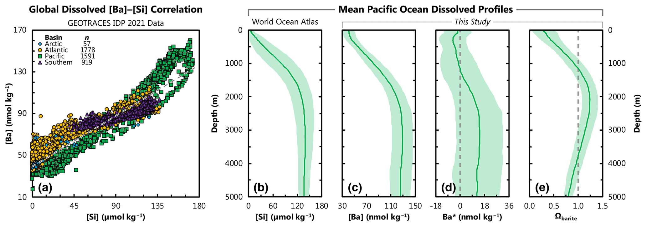
Figure 1Distribution of barium in seawater. (a) Property–property plot showing the 4345 co-located, core-feature-complete dissolved data used in ML model training (Sect. 2). Sample locations shown in Fig. 2. Dashed line shows best-fit linear regression through these data, whereby [Ba] = 0.54 ⋅ [Si] + 39.3. Panels (b), (c), (d), and (e) show average Pacific Ocean dissolved depth profiles of [Si], [Ba], Ba*, and Ωbarite, respectively. Solid line denotes the arithmetic mean, and the shaded region encompasses 1 standard deviation either side of the mean. Dashed line indicates Ba* = 0 (d) and Ωbarite=1 (e).
While the Ba-based proxies are valuable, their applications are potentially limited by insufficient knowledge of the distribution of [Ba]. For example, there is significant vertical and spatial variability in the Ba–Si relationship (Sect. 3.3; Fig. 1), which we quantify using Ba* (barium star; e.g., Horner et al., 2015; Sect. 3.3):
where [Ba]predicted is based on the Ba–Si linear regression (Fig. 1):
Here, [Si]in situ has units of micromoles per kilogram (µmol kg−1) and [Ba]predicted nanomoles per kilogram (nmol kg−1); therefore, Ba* also has units of nmol kg−1. The vertical profile of Ba* is rarely conservative (Fig. 1d), and these variations could introduce uncertainty in the reconstruction of [Si] using Ba.
The relationship between sedimentary BaSO4 accumulation rates and productivity also contains a significant degree of scatter (e.g., Serno et al., 2014; Hayes et al., 2021). Some of this scatter may relate to variability in BaSO4 preservation, which is at least partially sensitive to the ambient saturation state, Ωbarite (e.g., Schenau et al., 2001; Singh et al., 2020; Fig. 1). The saturation state of a parcel of water with respect to BaSO4 is defined as follows:
where Q is the Ba and sulfate ion product, and Ksp is the in situ BaSO4 solubility product. Discerning the importance of Ωbarite to BaSO4 preservation has hitherto been challenging owing to the sparsity of in situ [Ba] measurements. Accurately determining the global distribution of [Ba] would be valuable for geochemists and oceanographers and would enable a more thorough investigation of the effects of preservation on BaSO4 fluxes and a refinement of the Ba–Si nutrient proxy.
A powerful way of interrogating oceanic element distributions is through modeling. Broadly, there are two modeling approaches relevant for simulating [Ba]: mechanistic (i.e., theory driven) and statistical modeling (i.e., data driven; e.g., Glover et al., 2011). In mechanistic or process-based modeling, model outputs are derived from sets of underlying equations that are based on fundamental theory. As such, mechanistic model outputs can be interrogated to obtain an understanding of processes and their sensitivities. However, creating a mechanistic model of the marine Ba cycle requires embedding a biogeochemical model of BaSO4 cycling within a computationally expensive global circulation model. Although the computational cost associated with building mechanistic models has been reduced by the development of ocean circulation inverse models (e.g., DeVries, 2014; John et al., 2020), this approach still requires detailed parameterizations of the marine Ba cycle, which do not currently exist. In contrast, statistical models are based on extracting patterns from existing data and using those relationships to make predictions. Statistical models encompass a wide variety of approaches ranging from regression analysis to machine learning (ML). Of particular interest to our study are ML models, which can make predictions without any explicit parameterizations of causal relationships. Machine learning models are computationally efficient and can be highly accurate, though they offer limited interpretability. Machine learning is increasingly being used to solve problems in Earth and environmental sciences, including simulating the dissolved distribution of tracers in the sea (e.g., for cadmium, Roshan and DeVries, 2021; copper, Roshan et al., 2020; iodine, Sherwen et al., 2019; nitrogen isotopes of nitrate, Rafter et al., 2019; and zinc, Roshan et al., 2018).
The goal of this study is to obtain an accurate global simulation of [Ba], which ML makes possible even in the absence of a process-level understanding of the marine Ba cycle. We tested thousands of ML models that were trained using quality-controlled GEOTRACES data from the Arctic, Atlantic, Pacific, and Southern oceans, supplemented by Argo, satellite chlorophyll, and bathymetry data products (Sect. 2). Models were tested for their accuracy by simulating [Ba] in the Indian Ocean and comparing predictions against observations made between 1977–2013. Since no Indian Ocean data were seen by any of the models during training, we are able to identify models with high generalization performance (Sect. 3). We then identify an optimal set of predictor variables; calculate model uncertainties; and simulate [Ba], Ba*, and Ωbarite on a global basis (Sect. 5). This result will be valuable for researchers interested in marine Ba cycling and demonstrates the utility of ML in tackling problems in marine biogeochemistry.
Machine learning algorithms are adept at making accurate predictions of a target variable by identifying relationships between variables within large datasets. However, making accurate predictions first requires that an ML algorithm is trained on existing observations of that variable alongside a number of other parameters. These other parameters, hereafter termed features, are an important part of model training. Features should encode information that may help the ML algorithm predict [Ba]; otherwise their inclusion may diminish model performance. Features should also be well characterized in the global ocean, which allows ML models to make predictions in regions beyond the initial training dataset. We selected 12 model features by considering the trade-off between feature availability and presumed predictive power (Table 1). While testing more features may have resulted in a more accurate final model, we found that many observations of [Ba] did not have corresponding data for multiple features; thus, including more features would have meant fewer training data. Moreover, we find that including more than nine features can actually diminish model performance. As such, we did not evaluate the predictive power of other features beyond the 12 initially selected.
Table 1List of oceanographic parameters selected as model features. The features tested were selected based on their presumed predictive power and high geospatial coverage.
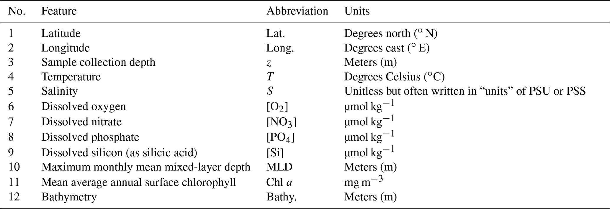
The 12 features used to predict [Ba] and their associated data sources are summarized in Table 1 and described below. The first three features (latitude, longitude, and depth) record geospatial information that defines the location of an observation in three-dimensional space. To avoid numerical discontinuities, latitude and longitude were introduced into the model as a hyperparameter consisting of the cosine and sine of their respective values (in radians). Data for features 1–3 were included in the sample metadata. Features 4–9 encode physical (temperature and salinity) and chemical (oxygen and nutrients) information that is routinely measured alongside [Ba]. These data were generally available for the same bottle as the [Ba] measurements; however, when that was not the case, nutrient data were taken from the corresponding location during a separate cast or, in the case of oxygen, from linearly interpolated sensor data. The final three features are independent of depth, meaning that all samples within a given vertical profile exhibit the same value for MLD (mixed-layer depth), sea surface chlorophyll a, and bathymetry. Features 10–12 were drawn from several data sources. A climatology of MLD (feature 10) was compiled using the Argo database (Holte et al., 2017). We selected maximum monthly mean MLD as the feature of interest as this appears to be the spatiotemporal scale most relevant for influencing [Ba] distributions (Bates et al., 2017). Feature 11 represents a blended Sea-viewing Wide Field-of-view Sensor and Moderate Resolution Imaging Spectroradiometer climatology of chlorophyll a that was obtained from the Copernicus Marine Environment Monitoring Service (CMEMS, 2021). We calculated the mean annual chlorophyll a for each grid cell in the data product and log-transformed the data to reduce parameter weighting (e.g., Rafter et al., 2019). Data for MLD and chlorophyll a were extracted at the location of [Ba] observations using nearest-neighbor interpolation, and their values were logged in the master record. Bathymetric information (feature 12) was extracted from one of two sources. Our preferred source was the sample metadata, which generally included a value for bathymetry. For samples lacking bathymetric information, we used nearest-neighbor interpolation to extract a value from the ETOPO5 Global Relief Model (National Geophysical Data Center, 1993). Occasionally, the ETOPO5-extracted bathymetry was shallower than the deepest observation of [Ba] in a given vertical profile. In such cases, the bathymetry logged in the master record was set to 1.01 times the depth of the deepest observation in that profile.
The [Ba] data from the Indian Ocean were collected from several, primarily pre-GEOTRACES sources (Table 2). As such, these data were generally incomplete for the 12 features used to train the ML models. Rather than using a mixture of in situ and interpolated data, we decided to interpolate all Indian Ocean data for parameters 4–12. Data for parameters 4–9 were linearly interpolated from the nearest vertical profile in the World Ocean Atlas 2018 (WOA; Boyer et al., 2018; García et al., 2018a, b; Locarnini et al., 2018; Zweng et al., 2018), and values for MLD and chlorophyll a were extracted from the aforementioned data products using nearest-neighbor interpolation. Bathymetric information was obtained from either the WOA or ETOPO5. For the vast majority of the samples, bathymetry was taken as the arithmetic mean of the maximum depth of the nearest vertical profile in the WOA and the depth at the standard level below. For example, if the maximum depth at a station was 950 m, the bathymetry was recorded as 975 m, which is the mean of levels 46 (950 m) and 47 (1000 m). For profiles with a maximum depth of 5500 m (level 102, the deepest in the WOA), bathymetry was recorded as either 5550 m or the nearest-neighbor-interpolated value from ETOPO5, whichever was deeper.
Table 2Data sources. Information regarding the source of [Ba] incorporated into the master record.
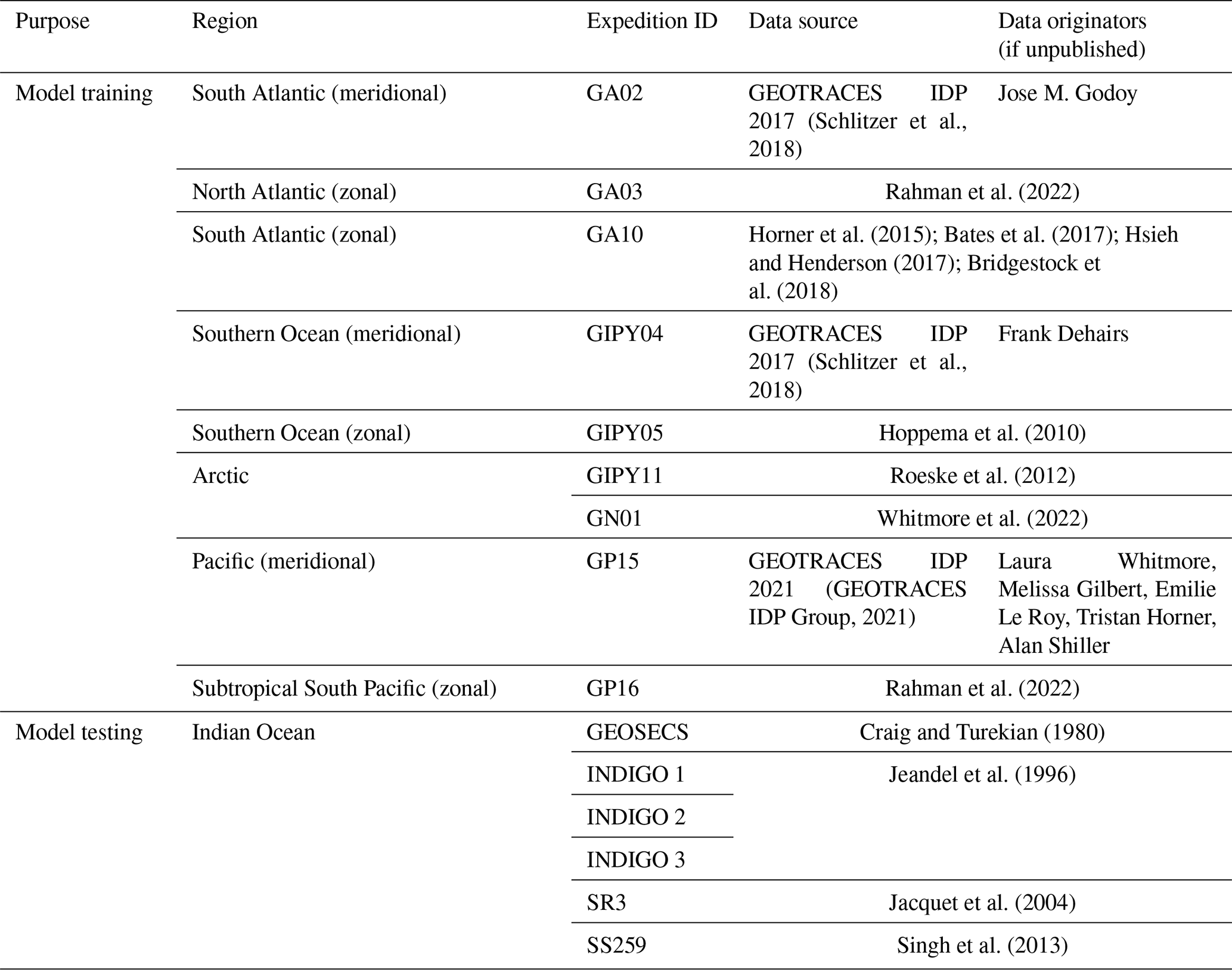
This data ingestion process resulted in a master record containing 5502 observations of [Ba] that also contained a corresponding value for all 12 core features (Table 1). The record was then split into a Pareto partition: the first partition was used for ML model training (4345 observations, 79 % of data; Fig. 1a), and the second was used for model testing (1157 data; 21 %). This partitioning was determined based on the basin from which the sample was collected; data from the Arctic, Atlantic, Pacific, and Southern oceans were used in model training, whereas the 1157 [Ba] observations from the Indian Ocean were reserved for model testing (Table 2; Fig. 2). This location-based separation of training and testing data was chosen to minimize overfitting, which can occur when the training–testing separation is randomly assigned (see Sect. 3.2).
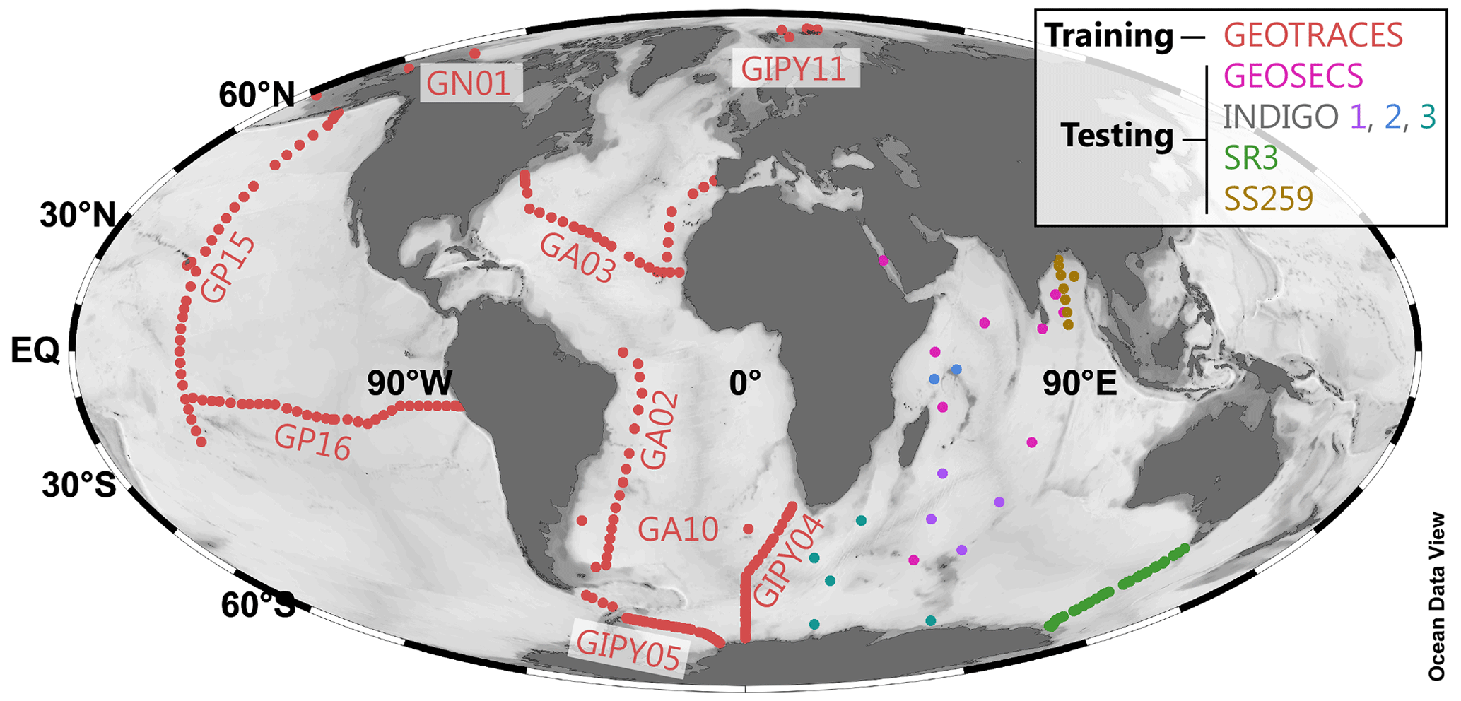
Figure 2Geographical distribution of the training and testing data. The 4345 items of core-feature-complete training data (red; Fig. 1) are from the GEOTRACES 2021 Intermediate Data Product (GEOTRACES IDP Group, 2021); GEOTRACES expedition identifiers are noted next to each section. The n=1157 testing data items from the Indian Ocean are color-coded by expedition. Data sources listed in Table 2.
In the following subsections, we discuss details of the specific ML algorithm that was used for model development (Sect. 3.1), explain the model training and testing process (Sect. 3.2), and describe how a global prediction of [Ba] was obtained and interrogated (Sect. 3.3).
3.1 Algorithm selection and training
We opted for supervised ML using a Gaussian process regression learner, implemented in MATLAB. This particular ML algorithm is non-parametric, kernel-based, and probabilistic, which means that it does not make strong assumptions about the mapping function, can handle nonlinearities, and takes into account the effect of random occurrences when making predictions. Gaussian process regression algorithms are widely used in geostatistics, where they are often referred to as kriging (e.g., Cressie, 1993; Rasmussen and Williams, 2006; Glover et al., 2011). This type of algorithm is ideal when working with continuous data that also contain a certain level of noise, such as from measurement uncertainty or oceanographic variation. The MATLAB function fitrgp was used for model training. A full list of the parameter selections used in fitrgp is provided in Table S1 in the Supplement. All predictors were normalized and standardized to have a mean of zero and a standard deviation of unity. This process places all parameters on the same relative range and reduces scale dependencies.
A selection of the training data were used to train 4095 different machine learning models with the goal of finding a model that could accurately simulate the global distribution of [Ba]. The number of models derives from the number of features investigated, whereby each model uses a unique combination of the 12 features in Table 1 and our testing followed a factorial design whereby each feature was either enabled or disabled. This design yields a total of 212 unique feature combinations (i.e., levelsfeatures); however, since it is not possible to train a model with zero features enabled, the final number of unique, trainable, ML models with ≥ 1 features is 212–1 = 4095. The full experiment list is provided in Horner and Mete (2023). Each of the 4095 models was trained using the same training dataset and with the same function parameters described in Table S1 in the Supplement.
3.2 Assessing model performance
Model performance – accuracy and generalizability – was assessed during two phases: training and testing. During model training, the 4345 observations of [Ba] from the Arctic, Atlantic, Pacific, and Southern oceans were randomly split into two folds: a training fold containing 80 % of the observations and a holdout fold containing the other 20 %. Model accuracy was assessed by comparing model-predicted [Ba] against observed [Ba] for the 20 % of the data in the holdout fold. We then performed additional testing to establish model generalizability. A significant problem in supervised ML, and particularly in Gaussian process regression learning, is overfitting: models may fit the noise in the training data, leading to poor generalization performance (Rasmussen and Williams, 2006). Since our goal was to develop a global model of [Ba] using regional training data, we deemed it especially important to identify generalizable models. Generalizable models were identified through a testing process involving regional cross-validation; each trained model was used to predict [Ba] for the 1157 samples from the Indian Ocean, and model predictions were again compared against observations. Importantly, no [Ba] data from the Indian Ocean were seen by any of the models during training. This process helped to identify models that may have been overfit to the training data and can further be used to calculate generalization errors (Sect. 4.1).
The accuracy of trained models was determined by comparing ML model predictions against withheld data and calculating the mean absolute error (MAE) and mean absolute percentage error (MAPE), defined as follows:
and:
respectively, where n is the sample size.
Models with lower accuracy exhibit higher errors, whereas models with high accuracy have lower errors. We calculated MAE and MAPE for every possible feature combination, which enables quantification of how specific features affect model performance. Likewise, we calculated errors for each model based on predictions made during training (i.e., for the holdout fold) and during model testing (i.e., during regional cross-validation; Fig. 3). This information is used to quantify generalization performance; low errors for both training and testing indicate models that are both accurate and generalizable, whereas models with low training errors and high testing errors might indicate models that are overfit to the training data.
3.3 Global predictions
A select number of models with low MAE and MAPE were used to simulate [Ba] on a global basis. The process by which we selected these models is described in Sect. 5.1. Global simulations were performed on the same grid as the WOA, which was also used as the data source for features 1–9 (Boyer et al., 2018). The WOA is a 1∘ × 1∘ resolution data product with around 41 000 stations that contain up to 102 depth levels spanning 0–5500 m in 5, 25, 50, or 100 m increments. Data for features 10–12 (MLD, chlorophyll a, and bathymetry) were also resampled to the WOA grid using the same sources and interpolation methods as described for the Indian Ocean testing data in Sect. 2. Model outputs were visualized using Ocean Data View software (ODV; Figs. 5–8; Schlitzer, 2023).
A selection of the most accurate models of [Ba] was used to simulate Ba* and Ωbarite. Star tracers, such as Ba*, are valuable for illustrating processes that influence the cycling of elements in the ocean. First defined for N–P decoupling (N*; Gruber and Sarmiento, 1997), star tracers show variations whenever there are differences in the sources and sinks of the two elements being compared. If there are no differences in sources and sinks for either element, the tracer will show conservative behavior because both elements share the same circulation. Barium star is based on Ba–Si decoupling and was first defined by Horner et al. (2015). The definition of Ba* is shown in Eqs. (1) and (2). The coefficients in Eq. (2) are based on data from the GEOTRACES 2021 Intermediate Data Product and specifically the subset of these data shown in Fig. 1. These coefficients differ from previous formulations of Ba* that were based primarily on [Ba] and [Si] data from the Southern and Atlantic oceans (e.g., Horner et al., 2015; Bates et al., 2017). The global distribution of Ba* was determined in two steps. First, [Si]in situ from the WOA 2018 (García et al., 2018b) was used to calculate [Ba]predicted using Eq. (2). Next, values of [Ba]in situ were taken from ML model output and Ba* calculated using Eq. (1).
Values of Ωbarite were computed using the method described by Rushdi et al. (2000), summarized in Eq. (3). The numerator, Q, represents the in situ Ba and sulfate ion product and, in this formulation, depends only on Ba and sulfate molality. The denominator, Ksp, depends on T, S, and z (i.e., pressure) and is calculated in two steps: in situ T and S are used to calculate the stoichiometric solubility product, and then this value is modified by calculating the effect of pressure on partial molal volume and compressibility, which are functions of T and z. As with the calculation of Ba*, values of in situ [Ba] were obtained from ML models, and co-located data for T, S, and z were extracted from the WOA (Locarnini et al., 2018; Zweng et al., 2018). Sulfate concentrations were assumed to be conservative with respect to S using [sulfate] = 29.26 mmol kg−1 when salinity = 35 PSU. This latter assumption likely breaks down in certain environments, such as where sulfate reduction occurs; accordingly, our model is not used to predict Ωbarite in restricted basins, such as the Black Sea or Caspian Sea. Given that our estimates of Ωbarite exhibit an MAE of 0.08 (Appendix), we believe that values of Ωbarite between 0.92 and 1.08 are indicative of equilibrium between BaSO4 and seawater.
Output from the most accurate ML models was then used to calculate mean [Ba] and Ωbarite for each basin, for a series of prescribed depth bins, and for the global ocean. This calculation was performed by weighting each cell in the model output by its volume, which ensures a fair comparison between any two points in the model output. We then subdivided the global ocean into five sub-basins: Arctic, Atlantic, Indian, Pacific, and Southern. Basin boundaries were defined as per Eakins and Sharman (2010), though we merged the Mediterranean and Baltic seas into the Atlantic and considered the South China Sea to be part of the Pacific Ocean. Neither [Ba] nor Ωbarite was simulated in the Black or Caspian seas, and thus these regions are not included in the global mean calculations.
4.1 Factors affecting model accuracy
Here we examine how model performance is influenced by the number and nature of features included during training. We consider model performance in terms of accuracy and generalizability, which we quantify using MAE (Eq. 4). We first explore how the number of features influences model performance (Fig. 3). Here we see that increasing the number of features generally improves the accuracy of trained models; however, the response differs depending on whether accuracy is calculated based on comparison to the holdout fold (i.e., during model training) or to the withheld Indian Ocean data (i.e., during model testing). When considering only the holdout fold, trained models predict [Ba] with a high level of accuracy, with the mean, median, and most accurate trained models achieve an MAE of 2.4, 1.7, and 1.3 nmol kg−1, respectively. Similarly, increasing the number of features almost always improves model accuracy; the MAE of the most accurate model for a given number of features decreases from 6.5 to 1.3 nmol kg−1 as the number of features is increased from 1 to 9, at which point MAE plateaus between 1.4–1.5 nmol kg−1 for models with 10–12 features (Fig. 3a).
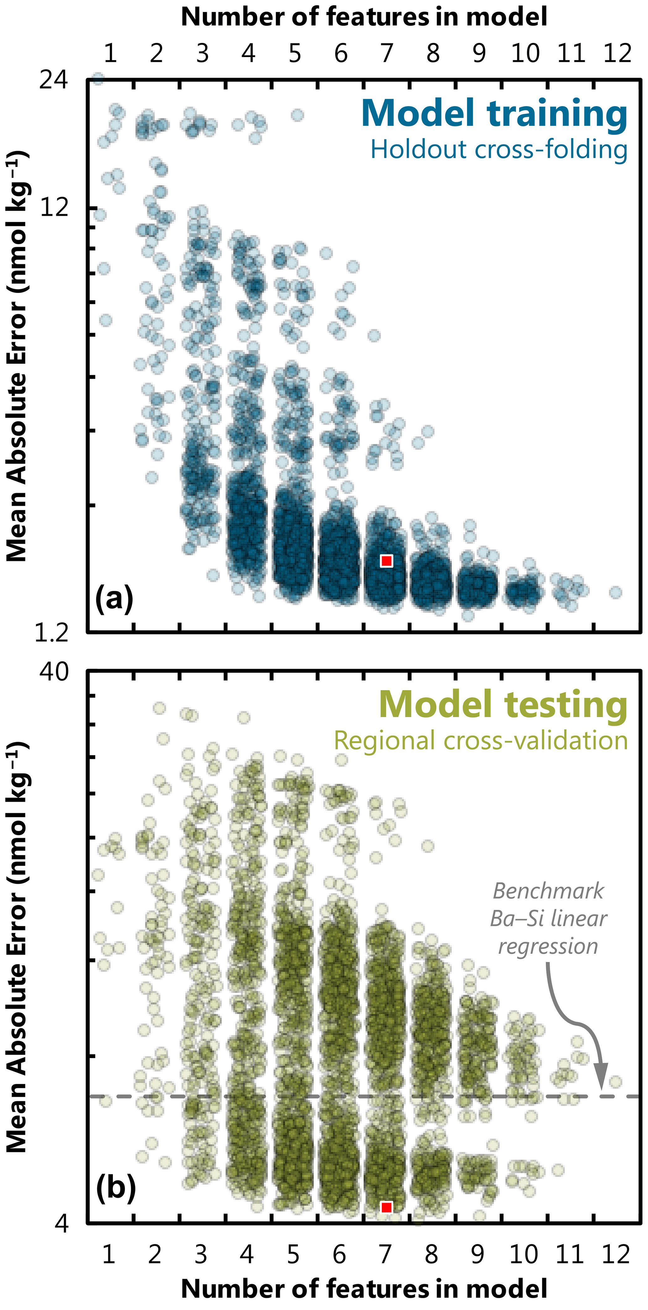
Figure 3Effect of feature addition on ML model accuracy. Accuracy was quantified for each of the 4095 trained models and quantified here using MAE (note log scale, which differs between panels). The accuracy of trained models is shown for random holdout cross-validation during training (a) and for regional cross-validation during testing (b). Square indicates the performance of our favored predictor model, no. 3080 (see Fig. 4, Sect. 5.1). The accuracy of the Ba–Si linear regression benchmark is shown as a dashed line in the lower panel (MAE = 6.8 nmol kg−1). To illustrate data density, points have been randomly positioned within their respective bin and plotted with 80 % transparency.
Moving to the regional cross-validation, the overall performance of models is lower; the same 4095 trained models achieve a mean, median, and most accurate MAE for the Indian Ocean dataset of 8.8, 7.9, and 4.0 nmol kg−1, respectively. For comparison, if [Ba] was estimated for these same 1157 Indian Ocean samples using the linear [Ba]–[Si] relationship (Fig. 1) and ambient [Si] as the only predictor, this linear model would achieve an MAE of 6.8 nmol kg−1. Thus, there are 1687 ML models that achieve a superior accuracy compared to existing methods for estimating [Ba], offering an improvement of as much as 41 % (Fig. 4). However, regional cross-validation also shows that the addition of more features may, in fact, degrade model performance. The MAE of the most accurate model for a given number of features decreases from 6.6 to 4.0 nmol kg−1 when the number of features is increased from one to eight. When the number of features is increased from 9 to 12, the MAE of the most accurate models increases monotonically from 4.1 to 7.1 nmol kg−1. The overall lower performance of trained models during regional cross-validation – and the observation that many of the feature-rich models perform worse than models with fewer features – is indicative of certain models being overfit to the training data. Together, these observations suggest that the optimum number of features needed to accurately predict [Ba] is between six and nine.
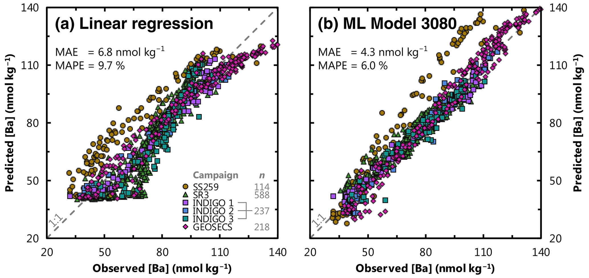
Figure 4Comparison of existing and ML methods to estimate [Ba] in seawater. Panel (a) shows the performance benchmark: predicted [Ba] for the Indian Ocean testing data using the [Ba]–[Si] linear regression and ambient [Si] as the sole predictor. Panel (b) shows predicted [Ba] using ML model 3080, which improves on existing methods by more than 37 %. Perfect correspondence between predictions and observations is indicated by the dashed line marked 1:1. Data locations and sources are shown in Fig. 2 and Table 2, respectively; n refers to the number of testing data for each campaign. Mean absolute error (MAE; Eq. 4) and mean absolute percentage error (MAPE; Eq. 5) are noted for both models.
We also evaluated the nature of the predictors used to estimate [Ba]. The full factorial experiment design enables us to perform comparisons between all models that contained a certain feature and all of those that did not (Sect. 3.1). We quantified the effect of adding a feature by comparing the absolute and percentage change in MAE relative to the mean MAE of the two sets of models. This comparison was performed three times: for all 4095 models based on the holdout cross-folded training data, for all models using the regionally cross-validated testing data, and again for the testing data but only considering those 1687 models that achieved a superior accuracy compared to the [Ba]–[Si] linear regression model (Table 3).
Table 3Feature addition analysis. Effect of each feature on model performance for training and testing datasets. Model performance is quantified using MAE; thus all columns have units of nanomoles per kilogram (nmol kg−1) unless otherwise shown. The testing analysis is further subdivided into a comparison of all models and good models, meaning those that achieved superior accuracy compared to the Ba–Si linear regression (Fig. 1).
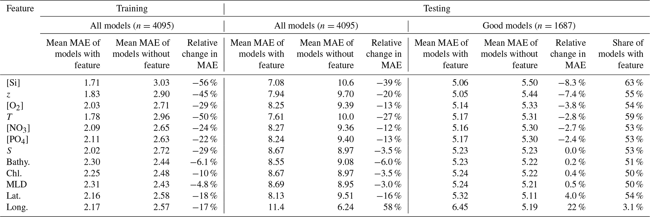
This analysis yields three main results. When considering only the holdout cross-folded training data, the addition of any of the 12 features improves model performance by between −4.8 % and −56 %. Except for longitude, similar across-the-board improvements were observed when considering only the testing data, though the improvements for most features were more modest (between −3.0 % and −39 %). When considering only the 1687 models that are superior to the [Ba]–[Si] linear regression model, six features improved model performance by −2.4 % to −8.3 % ([PO4], [NO3], T, [O2], z, and [Si]), five degraded model performance by +0.2 % to +22 % (bathy., Chl a, MLD, lat., and long.), and salinity had no significant effect (Table 3).
Overall, our results indicate that between six and nine features will result in an accurate and generalizable Gaussian process regression ML model of [Ba] and that [PO4], [NO3], T, [O2], z, [Si], and possibly S are likely to be included as predictors in such a model.
4.2 Model outputs
Almost 1700 models achieved superior accuracy compared to the Ba–Si linear regression benchmark of 6.8 nmol kg−1. We winnow this list to a single model, no. 3080, in the next section. We henceforth refer to model no. 3080 as our favored predictor model, which achieves an MAE of 4.3 nmol kg−1 using z, T, S, [O2], [PO4], [NO3], and [Si] as predictors (Fig. 4). Model no. 3080 is used to simulate [Ba], Ba*, and Ωbarite on a global basis and to calculate whole-ocean averages. Surface plots showing the model outputs for the sea surface, 1000, 2000, and 4000 m are shown in Figs. 5, 6, 7, and 8, respectively.
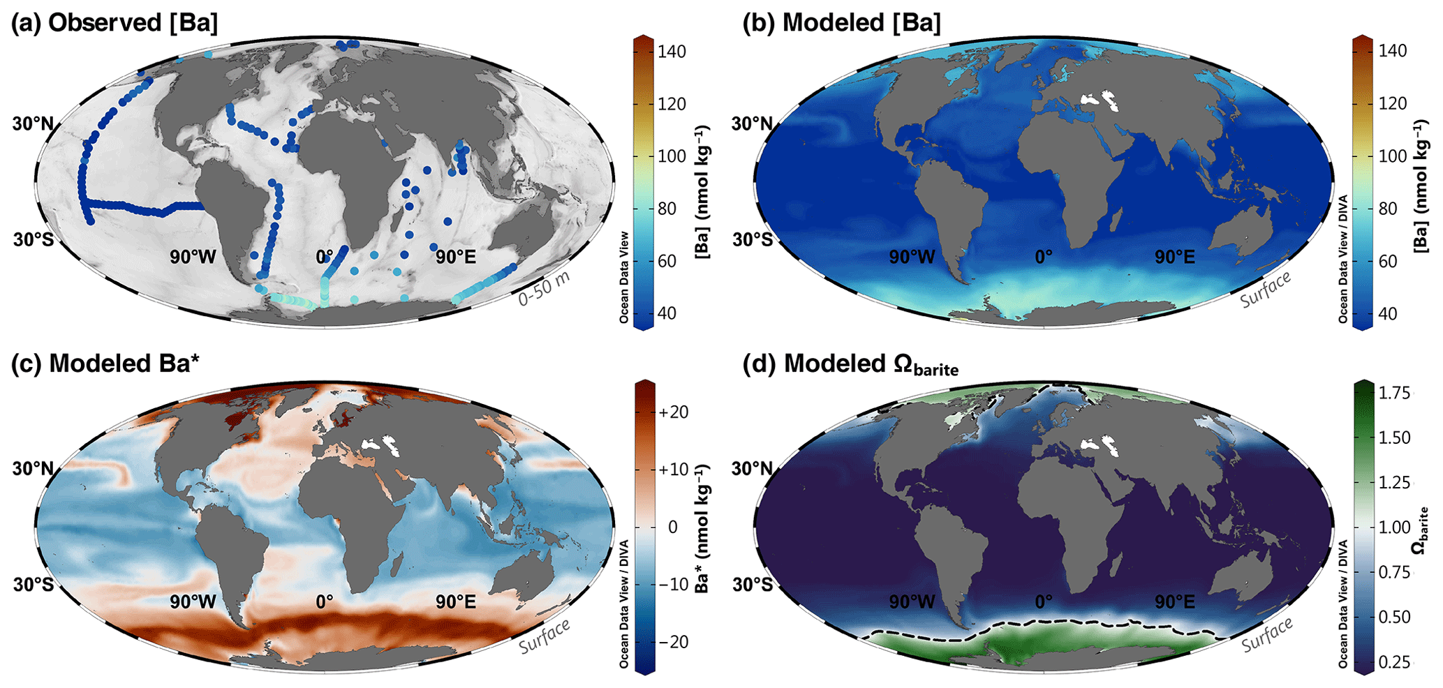
Figure 5Barium at the sea surface. Observed [Ba] between 0–50 m (a); model 3080 [Ba] (b), Ba* (c), and Ωbarite (d). The dashed line in panel (d) indicates the BaSO4 saturation horizon (i.e., Ωbarite=1.0). Panels (a) and (b) use the roma color map, whereas panels (c) and (d) use vik and cork, respectively (Crameri, 2018). Color palettes and parameter ranges are the same for the respective panels in Figs. 6–8.
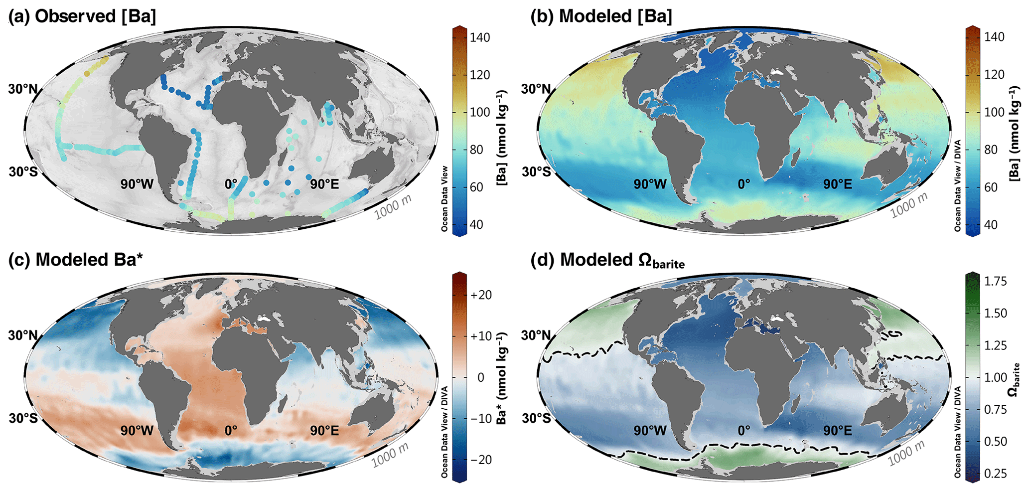
Figure 6Barium at 1000 m. Observed [Ba] (a); model 3080 [Ba] (b), Ba* (c), and Ωbarite (d). The dashed line in panel (d) indicates the BaSO4 saturation horizon.
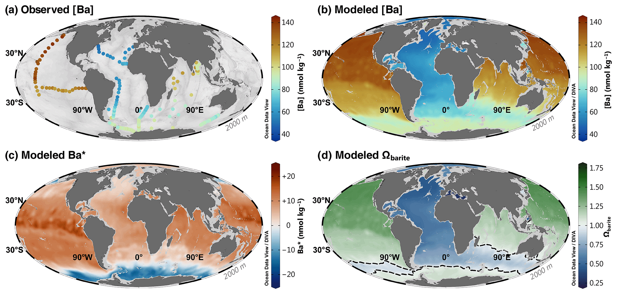
Figure 7Barium at 2000 m. Observed [Ba] (a); model 3080 [Ba] (b), Ba* (c), and Ωbarite (d). The dashed line in panel (d) indicates the BaSO4 saturation horizon.
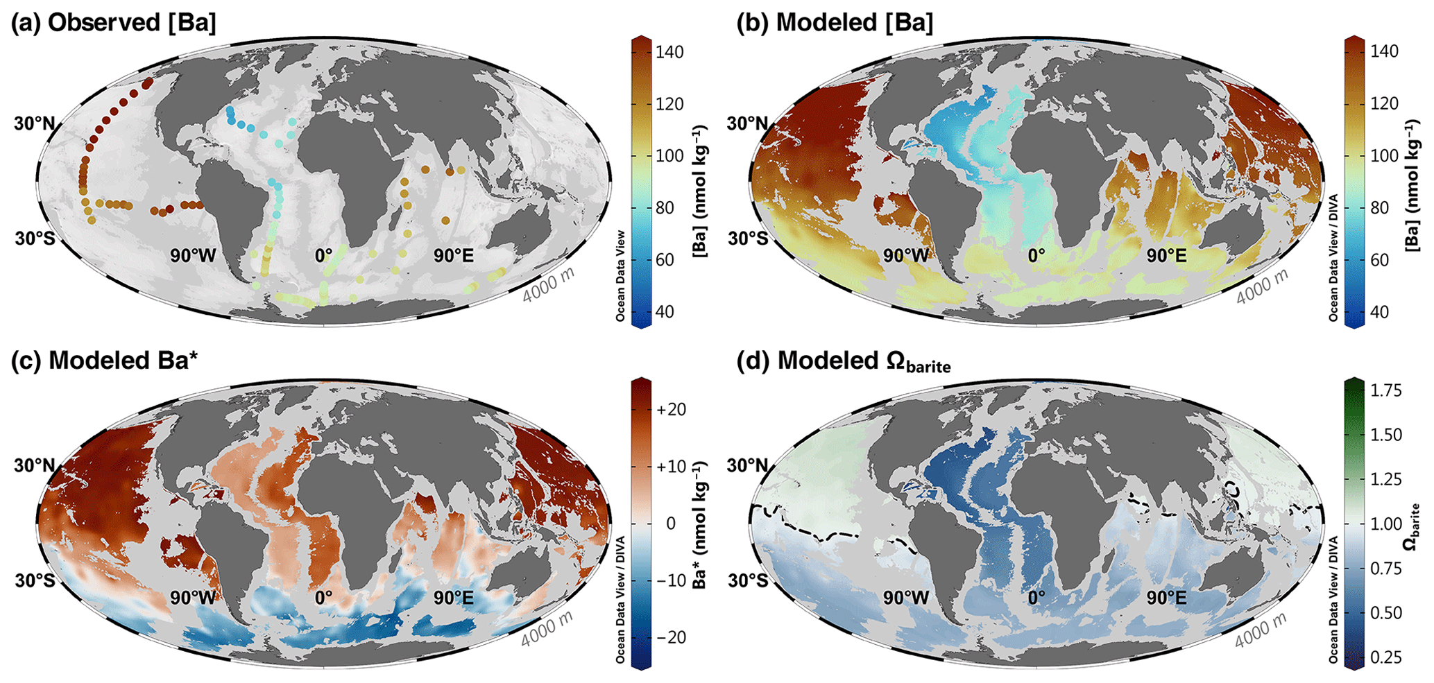
Figure 8Barium at 4000 m. Observed [Ba] (a); model 3080 [Ba] (b), Ba* (c), and Ωbarite (d). The dashed line in panel (d) indicates the BaSO4 saturation horizon.
Model no. 3080 contains 3 302 570 predictions each for [Ba], Ba*, and Ωbarite (Horner and Mete, 2023). Assuming that the MAPE and MAE are good estimates of the prediction error, we estimate that modeled [Ba] and Ba* have uncertainties of 6.0 % and 4.3 nmol kg−1, respectively. Uncertainties on Ωbarite were estimated by comparison to literature data, which yields an MAE of 0.08. These uncertainty estimates are discussed in more detail in Sect. 5.2 and the Appendix.
Modeled [Ba] ranges from 26.2 to 156.8 nmol kg−1, and the data exhibit an unweighted mean of 72.0 nmol kg−1. The range of model no. 3080 predictions is within the range of [Ba] encountered in the 4345 items of training data (17.1–159.8 nmol kg−1). This is an important consideration when assessing the accuracy of Gaussian process regression models, and we provide additional discussion of this point in the Supplement. Based on our formulation (Eqs. 1, 2), Ba* varies from −27.2 to +27.9 nmol kg−1 and possesses an unweighted mean of +2.4 nmol kg−1. Values of Ωbarite vary from 0.11 to 1.70 and exhibit an unweighted mean of 0.75. To account for the different volumes represented by each cell in the WOA grid, we constructed a volume-weighted mean of [Ba] and Ωbarite for the ocean as a whole, for each ocean basin, and for a series of prescribed depth bins (Fig. 9). Looking at the ocean as a whole, the probability density function of [Ba] roughly resembles a uniform distribution, with a mean ocean [Ba] of 89 nmol kg−1 (Fig. 9a). Within this mean is considerable spatial and vertical variation. For example, the Arctic Ocean exhibits the lowest volume-weighted mean [Ba] of 54 nmol kg−1, whereas mean Pacific [Ba] = 106 nmol kg−1. The Indian Ocean exhibits a similar mean [Ba] (90 nmol kg−1) to the mean of the global ocean. At depths shallower than 1000 m, [Ba] infrequently exceeds 100 nmol kg−1, whereas concentrations < 45 nmol kg−1 are rare below 1000 m (Fig. 9b).
The probability density function of volume-weighted Ωbarite is more similar to a normal distribution, albeit with a slight negative skew. Volume-weighted mean oceanic Ωbarite is 0.82. The Arctic, Atlantic, and Indian oceans are, on average, undersaturated with respect to BaSO4, all exhibiting mean Ωbarite≤0.82. In contrast, the Pacific and Southern oceans are within uncertainty of saturation, with mean Ωbarite of 0.97 and 1.04, respectively (Fig. 9c). Values of Ωbarite<0.2 are mostly restricted to the upper 250 m, whilst values of Ωbarite exceeding 1.5 are exceptionally rare, found only in the upper 1000 m of the Southern Ocean. Lastly, Ωbarite tends to increase between the 0–250, 250–1000, and 1000–2000 m depth bins, increasing from 0.42 to 0.65 and 0.96, respectively. Average Ωbarite in the deepest bin (2000–5500 m) is slightly lower, with a mean value of 0.92 (Fig. 9d). Given the accuracy of our model-derived Ωbarite predictions (0.08 to 0.10), the ocean between 1000–5500 m is at BaSO4 equilibrium, within uncertainty.
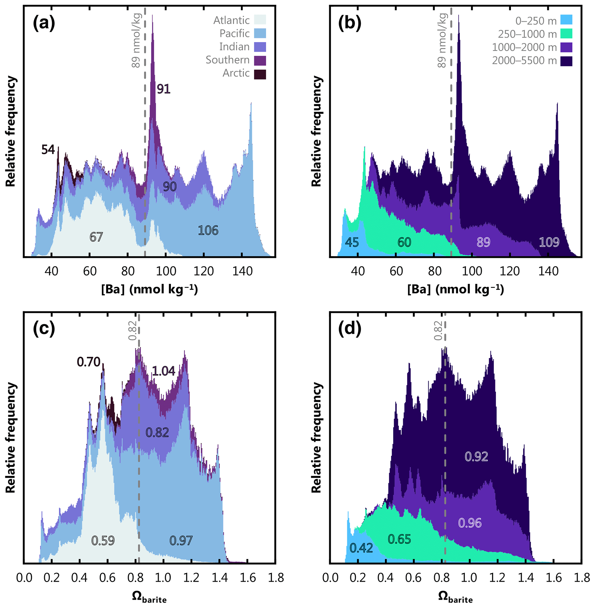
Figure 9Stacked, volume-weighted histograms showing the relative frequency distribution of dissolved [Ba] (a, b) and Ωbarite (c, d) in the global ocean. The left column shows data grouped by basin, and the right column shows data grouped by a prescribed depth bin. Numbers in each panel display the mean property value for that bin. Dashed line shows the global mean.
5.1 Identification of the optimal predictor model
Choosing a single, optimal model configuration is challenging given the sheer number of skillful ML models. Below we winnow the list from 4095 to a single model (no. 3080). We base our winnowing primarily on the results of the regional cross-validation performed in the Indian Ocean rather than on the errors determined from random holdout cross-folding of the training data. We believe that there are three strong reasons for winnowing in this way. First, Gaussian process regression learners tend to fit the noise in the training data, meaning that the training error is significantly lower than the generalization error (Rasmussen and Williams, 2006). Indeed, trained models showed overall lower performance during testing compared to during training, which we believe is evidence of overfitting (Fig. 3, Table 3). Second, a generalizable global model should be able to make predictions in regions where it has not already learned anything about the target variable. Our regional cross-validation approach satisfies this consideration since no Indian Ocean data were seen during model training. Third, the Indian Ocean is an ideal basin for testing as it exhibits the full diversity of features expected to influence [Ba] (riverine inputs, oxygen-minimum zones, coastal upwelling, etc.) and constitutes ≈ 20 % of the global ocean volume. Likewise, the Indian Ocean captures most of the range in [Ba] seen elsewhere in the ocean (Fig. 9); this likely reflects the input of Atlantic waters associated with the Agulhas retroflection, the transport of old Pacific waters via the Indonesian Throughflow, and the northward spreading of mode and intermediate waters from the Southern Ocean. We thus assume that the Indian Ocean testing errors are a good approximation of the generalization error, which we now use to winnow the list of models.
Our results show that 1687 of the 4095 ML models (41 %) produce more accurate predictions of [Ba] than the benchmark Ba–Si linear regression using [Si] as the sole predictor (Fig. 3, Table 3). We focus our winnowing on these 1687 models as they are superior compared to existing methods for estimating [Ba] in seawater. Focusing only on these good models reveals significant differences in the information content of the 12 features tested. For example, the inclusion of spatial information in the form of latitude and longitude significantly degrades mean model performance by between +4.0 % and +22 %, respectively. While bathymetry, chlorophyll a, and mixed-layer depth exhibited only minor influences, they were nonetheless deleterious to mean model performance by between +0.2 % and +0.5 % (Table 3). Only [PO4], [NO3], T, [O2], z, and [Si] consistently improved the mean ML model, which corresponds to model no. 3112 (testing MAE of 4.3 nmol kg−1). However, visual inspection of model no. 3112 output reveals that it does not reproduce expected nearshore surface plumes of elevated [Ba] close to certain major rivers (see Supplement). Though volumetrically minor, riverine inputs are a geochemically important component of the marine Ba cycle, and the existence of nearshore Ba plumes underpins a major proxy application of Ba. Nearshore riverine influence is easily discerned by low S; we thus explored output from model no. 3080, which is identical to model no. 3112 but includes S as a seventh feature during training. Model nos. 3080 and 3112 exhibit identical statistical performances for the testing data (MAE = 4.3 nmol kg−1; Fig. S1 in the Supplement) and make similar predictions for mean marine [Ba] and Ωbarite (89 nmol kg−1 and 0.82, respectively; see Supplement). The similar statistics for the two models are consistent with S exerting a near-negligible impact on overall model performance (Table 3). Despite this small effect, model no. 3080 is better able to reproduce riverine [Ba] plumes compared to model no. 3112 (see Supplement). We therefore consider model no. 3080 to be our best estimate of marine [Ba]. Model no. 3080 achieves a MAPE of 6.0 %, which represents a 39 % improvement over existing methods for estimating [Ba] (Fig. 4). We henceforth consider model no. 3080 to be our optimal predictor model, which we use to simulate [Ba], Ba*, and Ωbarite in Figs. 5–9.
5.2 Model validation
We now explore the validity of model no. 3080 in terms of its oceanographic consistency, the sources of uncertainty that affect its accuracy, and potential limitations of the model output. We find that model no. 3080 reproduces the major known features of the marine [Ba] distribution and makes testable predictions for regions that are yet to be sampled.
5.2.1 Visual inspection of model output
Visual inspection of model output is an important component of data analysis considering the limits of statistical tests (see, e.g., Anscombe, 1973). Models may produce statistically satisfactory fits to the testing data, but the oceanic realism of the output is also important to consider. Modeled [Ba] should display patterns consistent with related oceanographic properties and exhibit smooth vertical and spatial variations (Boyle and Edmond, 1975). Predicted [Ba] from model no. 3080 does indeed show smooth and systematic spatial and vertical variations that also resemble sparse observations (Figs. 4–8).
Model no. 3080 also shows systematic increases in [Ba] close to land, especially near the mouths of major rivers (Fig. 4). This is reassuring given that elevated sea surface [Ba] close to rivers is both widely reported and one of the major proxy applications of Ba: reconstructing spatiotemporal patterns of terrestrial runoff by measuring the Ba:Ca ratio of carbonates (e.g., Sinclair and McCulloch, 2004; LaVigne et al., 2016). For example, model no. 3080 correctly identifies elevated [Ba] near the Ganges–Brahmaputra (Singh et al., 2013), Río de la Plata (GEOTRACES IDP Group, 2021), and Yangtze outflows (Cao et al., 2021). Model no. 3080 also predicts elevated sea surface [Ba] in the Gulf of Guinea where several rivers discharge, including the Niger River; in the eastern tropical Atlantic associated with the Congo River (Edmond et al., 1978; Zhang et al., 2023); and in the Gulf of St. Lawrence (St. Lawrence River; see Supplement for additional details and figures). Except for the Congo River, these predictions of elevated nearshore [Ba] await corroboration. Interestingly, model no. 3080 does not predict elevated [Ba] at all major river mouths; neither the Mississippi River nor the Amazon River is associated with significant increases in sea surface [Ba] (see Supplement). The reasons for the lack of elevated [Ba] near the outflow of these two rivers is less clear. It is possible that the model is simply inaccurate in these regions, though we have no particular reason to believe that this is the case. Alternatively, it may reflect seasonal variations in Ba release that are not captured by our mean annual model (e.g., Joung and Shiller, 2014). It could also indicate that these particular rivers are not major net sources of Ba to the surface ocean, which might be the case if dissolved Ba is being retained in the catchment (e.g., Charbonnier et al., 2020) or estuary (e.g., Coffey et al., 1997).
Overall, model no. 3080 makes accurate, oceanographically consistent predictions of [Ba] in the Indian Ocean using input data from the WOA. Model no. 3080 also makes a number of testable predictions of [Ba] in regions lacking direct observations. Given that these predictions were made using the same model and the same WOA inputs, we believe that it is reasonable to assume that model no. 3080 output is an accurate representation of mean annual global [Ba].
5.2.2 Quantifying uncertainties
We now describe and, where possible, quantify two possible sources of uncertainty with regard to our ML model output. Before doing so, we describe how uncertainty is quantified and the uncertainty of existing approaches. Certain ML models, such as Gaussian process regression, offer low interpretability, meaning it is not possible to assess uncertainty using a conventional error propagation. Thus, all model uncertainties are assessed post hoc by comparing predictions against observations. Our preferred metrics are MAE and MAPE (Eqs. 4, 5). Existing approaches for estimating [Ba] result in a wide range of uncertainties. At the low end, the uncertainty associated with measuring [Ba] in seawater represents a fundamental limit to the accuracy of any model. A number of analysts report measurement uncertainties in the range of 1 %–2 % (e.g., Pyle et al., 2018; Cao et al., 2020). This level of intra-laboratory uncertainty is typical for [Ba] data obtained using isotope dilution–inductively coupled plasma mass spectrometry and applies to GEOTRACES-era datasets and to much of the testing data from the Indian Ocean. However, intra-laboratory uncertainty is typically much smaller than inter-laboratory uncertainty, which is often between 6 %–9 % (e.g., Hathorne et al., 2013). At the upper end, the benchmark Ba–Si linear regression achieves a MAPE of 9.7 % in the Indian Ocean (Fig. 4). Thus, useful ML models of [Ba] should achieve MAPE between 1 %–10 %. Indeed, our favored predictor model, no. 3080, achieves a MAPE of 6.0 %.
Now we consider two factors that contribute to the observed 6.0 % uncertainty: realization uncertainty and uncertainties in the training data. The realization uncertainty stems from the fact that two models trained on the same training dataset – even with the exact same subset of model features – will produce slightly different predictions. This is due to the holdout cross-folding process used during model training, which partitions the training dataset into random subsets (Sect. 3.1). The training process therefore results in a slightly different trained model each time the model is realized. We quantified the realization uncertainty by training select models 100 times and calculating the relative standard deviation of the different predictions of [Ba] for the 3.3 million values in the output. This uncertainty is small: the median, mean, and maximum realization uncertainties were 0.03 %, 0.04 %, and 0.32 % variability in modeled [Ba].
Next we consider uncertainties in the training data. As noted above, many labs report uncertainties in [Ba] measurements of 1 %–2 %, while inter-laboratory differences may be larger by up to a factor of 5. However, this does not consider any uncertainties associated with the other physical and chemical features used to predict [Ba]. In general, these supporting measurement uncertainties should be small: all overboard sensors are regularly calibrated, and biogeochemical properties in GEOTRACES are determined using established methods that are based on GO-SHIP best practices (Hood et al., 2010). Moreover, all GEOTRACES sections include crossover stations that are intended to facilitate intercalibration of all parameters, including those used here to predict [Ba] (Fig. 2; Cutter, 2013). The WOA, MLD, Chl a, and bathymetry data products are similarly subjected to stringent quality review, and so we consider it unlikely that these data contribute systematic biases. We believe that the most likely source of uncertainty relates to the fact that all predictor information used for model testing in the Indian Ocean was derived from time-averaged data products, whereas [Ba] was derived from in situ measurements. We made the decision to use time-averaged data products as predictors because the in situ data were incomplete for all 12 core features (Table 1). This limitation would have necessitated interpolation for some features and not others. Since all models were tested using the same predictor information, the comparison process should avoid systematic errors, though this does not preclude temporal variability, described next.
5.2.3 Other considerations
We now consider four other factors that potentially contribute to the uncertainty of the model output: short- and long-term temporal variations, limitations of ML, and uncertainties regarding the thermodynamic properties of BaSO4. Short-timescale variability in [Ba] may affect how models were evaluated, though this effect is difficult to quantify. All the models were trained using in situ physical and chemical data. Trained models should therefore be able to resolve seasonal variations in [Ba], so long as the models are also provided with seasonally resolved predictor information. However, model predictions in the Indian Ocean were made using annual average physical and chemical conditions and then evaluated by comparing these predictions against in situ [Ba]. The temporal mismatch between Indian Ocean observations and predictions is unlikely to be significant in the deep ocean, where seasonal variations are minor and the Ba residence time is longest (e.g., Hayes et al., 2018). Seasonal variations are, however, likely to matter more for the surface ocean. We were able to minimize some of the impact of these uncertainties by using long-term averages of Chl a and the maximum monthly mean MLD during model training and testing. Significant seasonal mismatches for other parameters are unavoidable given that [Ba] data are too sparse to develop a time-resolved model. We suspect that these variations are most likely to be significant for boundary sources rather than biogeochemical cycling of Ba; significant biogeochemical drawdown of surface [Ba] over seasonal timescales appears to be rare (e.g., Esser and Volpe, 2002), whereas there are large seasonal variations in river discharge that impact nearshore [Ba] (e.g., Samanta and Dalai, 2016). These suspicions could be tested using a model with a spatial resolution better than 1×1∘, which – in theory – is possible with model no. 3080 so long as similarly high-resolution data are provided for the seven predictors utilized by this model (z, T, S, [O2], [PO4], [NO3], and [Si]). While it is challenging to precisely quantify seasonal uncertainties, we note that model no. 3080 performs well at low [Ba], which is found mostly near the surface, where seasonal variations should exhibit the largest effects. Likewise, seasonal variations will have only a minor effect on our calculations of global mean [Ba] or Ωbarite (Fig. 8).
Long-term variability in [Ba] may also influence model performance since the testing data from the Indian Ocean were collected between 1977 (GEOSECS) and 2008 (SS259; Fig. 2). If secular changes in Indian Ocean [Ba] were occurring, we might expect models to make accurate predictions for some datasets at the expense of others. In contrast, we note that model no. 3080 reproduces all testing datasets similarly well, with the exception of a subset of samples from SS259 in the deep Bay of Bengal. Here we observe that model no. 3080 predicts 18 % higher [Ba] than that observed by Singh et al. (2013) for the 42 samples between 1000–3000 m (Figs. 4b; 7a, b). Interestingly, model no. 3080 correctly predicts [Ba] at nearby GEOSECS stations 445 and 446, also in the Bay of Bengal, sampled some 31 years prior to SS259. We briefly consider three possibilities for the origin of this regional model–data discrepancy. It may derive from the fact that model no. 3080 does not include the features needed to correctly predict [Ba] in these samples. We view this as the least likely possibility as model no. 3080 performs well for other samples from the northern Indian Ocean, including for samples shallower than 1000 m from Singh et al. (2013). Another possibility is that it could reflect an 18 % decrease in [Ba] in the deep Bay of Bengal since the GEOSECS survey in the 1970s. Lastly, it could reflect differences in how in situ [Ba] was measured, noting that Singh et al. (2013) opted for standard addition instead of isotope dilution. We currently lack the data needed to confidently distinguish between these latter two possibilities.
A third factor concerns the limitations of ML itself. We note that no trained model was able to achieve a MAPE better than ∼ 6 %. This 6 % value may represent one of three things. First, it may point toward an intrinsic limitation of Gaussian process regression. Other types of ML, such as decision trees or artificial neural networks, may be able to achieve superior accuracy, though this was not investigated. Second, it may indicate that the 12 features investigated provide insufficient information about [Ba] to achieve higher accuracy. We view this as unlikely given that our earlier analysis showed that only 6–9 features were needed to accurately simulate [Ba] and that the 12 features tested have proven useful in other studies simulating dissolved tracer distributions (e.g., Rafter et al., 2019; Sherwen et al., 2019; Roshan and DeVries, 2021). However, this does not rule out the existence of other features beyond the 12 that we tested and that are more useful for predicting [Ba]; it is only that we did not investigate them. Third, it is possible that the lowest MAPE of ∼ 6 % reflects the current limit of inter-laboratory uncertainty in determining [Ba]. We note that inter-laboratory uncertainties of 6 %–9 % were reported for the measurement of Ba:Ca in carbonates (n=10 labs; Hathorne et al., 2013). If the ∼ 6 % MAPE derives from inter-laboratory uncertainty, it is unlikely that further model refinements will improve the accuracy of [Ba] predictions: the fundamental limitation is the data, not the model.
A final source of uncertainty concerns the computation of Ωbarite, which contains two further sources of uncertainty: the thermodynamic model and the solubility coefficients used to calculate Ksp. We calculated Ωbarite based on the computation described by Rushdi et al. (2000), and our approach yields similar values to their study and several others (e.g., Jeandel et al., 1996; Monnin et al., 1999; see Appendix). The model used by Rushdi et al. (2000) is based on BaSO4 solubility data from Raju and Atkinson (1988), who note good agreement with the thermodynamic data of Blount (1977). These solubility data were obtained based on experimentation with lab-made, coarse-grained BaSO4, which is unlikely to be wholly representative of the microcrystalline BaSO4 precipitates found in seawater. Thus, the absolute values of Ωbarite calculated here may be subject to eventual revision; however, the vertical (Fig. 1), spatial (Figs. 4–8), and whole-ocean (Fig. 9) trends in Ωbarite are robust. Should new thermodynamic data for marine-relevant micron-sized pelagic BaSO4 become available, updated maps of Ωbarite could be recalculated using model-3080-derived [Ba] data. Given the nature of these uncertainties, we opted to calculate prediction uncertainties for Ωbarite empirically by comparison to literature data (see Appendix). This yields a value between 0.08 and 0.10, which is similar to the 10 % prediction error reported by Monnin et al. (1999).
5.3 Barium in seawater: a global perspective
Here we provide an overview of the main model features in [Ba], Ba*, and Ωbarite, then outline three possible applications of the model output.
5.3.1 Dissolved distribution of [Ba]
Model no. 3080 predictions show several interesting features in [Ba] (Figs. 5–8). The model reproduces the expected nutrient-like distribution of [Ba] (Fig. 1c) and shows a general increase in [Ba] along the meridional overturning circulation: volume-weighted mean [Ba] increases from 67 to 90 to 106 nmol kg−1 from the Atlantic to Indian to the Pacific Ocean, respectively. The model also predicts some variation in shallow [Ba] that follows major surface water currents, such as a region of elevated [Ba] associated with the North Pacific Current, as well as low [Ba] in the western North Atlantic associated with the Gulf Stream (Fig. 5b; Talley et al., 2011). However, these features and the processes driving them await corroboration.
Considering the ocean as a whole, we can use our model to calculate the total Ba inventory of seawater. Using the mean oceanic [Ba] of 89 nmol kg−1 and multiplying by the mass of seawater (1.37×10²¹ kg) yields a total inventory of 122±7 Tmol Ba, whereby the uncertainty is based on the MAPE of model no. 3080 (6.0 %). This estimate of the total oceanic Ba inventory is between 11 %–21 % lower than existing estimates of 145 Tmol Ba (Dickens et al., 2003; Carter et al., 2020). Given the range of probable global marine Ba fluxes between 18 (Paytan and Kastner, 1996) and 44 Gmol Ba yr−1 (Rahman et al., 2022), our inventory estimate places the mean residence time of Ba in seawater between 2600–7200 years.
5.3.2 The Ba–Si relationship
We now quantify spatial and vertical variations in the Ba–Si relationship, which we explore using Ba*. Star tracers, such as Ba*, highlight the processes affecting the distribution of an element by comparing it to another tracer that shares the same circulation. Originally described to explore global patterns of nitrogen fixation and denitrification (Gruber and Sarmiento, 1997), the concept has since been extended to study the processes affecting the distributions of many other bioactive elements, including Si (Si*, relative to N; Sarmiento et al., 2004), cadmium (Cd*, relative to P; Baars et al., 2014), and zinc (Zn*, relative to Si; Wyatt et al., 2014). First defined by Horner et al. (2015) for Ba, Ba* is analogous to other star tracers: it is a measure of Ba–Si decoupling whereby larger values indicate larger Ba–Si deviations relative to expected mean ocean behavior. Vertical or spatial differences in Ba and Si sources or sinks will drive variations in Ba*, as will any Ba:Si fractionation occurring during their combined cycling. Conversely, if all Ba and Si cycling occurs in the same places (and with a fixed Ba:Si ratio), no Ba–Si decoupling will occur, and Ba* will exhibit conservative behavior. Since Ba and Si are cycled by different processes and since there are large vertical and spatial variations in the intensity of these processes (e.g., Bishop, 1989), significant variations in Ba* are possible. We now explore these variations.
In the surface ocean, patterns of Ba* generally resemble those of [Ba] (Fig. 4). In large parts of the ocean, surface [Si] approaches 0 µmol kg−1; thus, variations in Ba* derive mostly from variations in [Ba]. This is most evident when examining regions with significant terrestrial input of Ba, such as from major rivers (Sect. 5.2.1) and from rivers and continental shelves in the Arctic (e.g., Guay and Falkner, 1998; Whitmore et al., 2022; Fig. 5a). The Southern Ocean also exhibits positive Ba*, though we suspect the mechanism is different. Here we observe a belt of waters with positive Ba* 20 nmol kg−1 centered on the Polar Frontal Zone – the region between the Antarctic Polar Front and the Subantarctic Front (Orsi et al., 1995; Fig. 5a). Silicic acid is intensely stripped from waters that transit northward through this region (e.g., Sarmiento et al., 2004), potentially contributing to elevated Ba* at the sea surface. Dissolved [Ba] and Ba* then decrease to the north of the Subantarctic Front, partly driven by extensive particulate Ba formation in the frontal region (e.g., Bishop, 1989).
At 1000 m, the Atlantic, South Pacific, and southern Indian oceans exhibit positive Ba* around +10 nmol kg−1, whereas the North Pacific, Southern, and northern Indian oceans are negative between −10 and −20 nmol kg−1 (Fig. 6c). The positive anomalies are likely to be related to the northward spreading of southern-sourced intermediate waters that originate within the Polar Frontal Zone and carry positive Ba* into the low latitudes (e.g., Bates et al., 2017). In the Atlantic, these values are carried all the way to the north of the basin and return as North Atlantic Deep Water with only minor modifications to Ba* (10 nmol kg−1; Figs. 6c, 7c, 8c). Negative Ba* in the North Pacific, Southern, and northern Indian oceans at 1000 m likely reflects a mixture of hydrographic processes and in situ processes. For example, the extensive region of negative Ba* in the North Pacific is closely associated with North Pacific Intermediate Water, which originates in the Sea of Okhotsk (Talley, 1991). While the specific mechanism sustaining this particular Ba* feature is unknown, it most likely reflects a combination of preferential removal of Ba relative to Si in the source water formation region (such as from particulate Ba formation) and weak vertical mixing in the subsurface North Pacific relative to lateral transports (e.g., Kawabe and Fujio, 2010). We suspect that the negative Ba* values seen above 1000 m in the northern Indian Ocean originate through processes occurring internally within this basin as the majority of the Indian Ocean below 1000 m exhibits positive Ba*. A possible mechanism for these shallow negative Ba* anomalies may relate to the relatively weak overturning transports (Talley, 2008) and the strong particulate Ba cycle north of 30∘ S (Singh et al., 2013), though this awaits more detailed investigation.
Lastly, the Southern Ocean exhibits negative Ba* between −10 and −20 nmol kg−1 from ≈ 200 m water depth to the seafloor. These negative anomalies in Ba* appear to be associated with Circumpolar Deep Water and, below that, Antarctic Bottom Water; the influence of the latter can also be seen in near-bottom negative Ba* in the South Pacific, southern Indian, and South Atlantic oceans (Fig. 8c). As with the other basins, the origin of the negative Ba* waters in the Southern Ocean likely reflects a combination of in situ and circulation-related phenomena. For example, in the Southern Ocean, Si is only stripped at the very surface, whereas particulate Ba formation is thought to be greatest in the mesopelagic (i.e., between 200–1000 m; e.g., Stroobants et al., 1991). Barite formation is generally considered to be related to the regeneration of particulate organic matter (e.g., Chow and Goldberg, 1960), whereby the former consumes Ba, and the latter releases Si. Thus, intense organic matter remineralization and associated pelagic BaSO4 precipitation could contribute to negative Ba* in the mesopelagic Southern Ocean. Similarly, the Si cycle in the Southern Ocean tends to trap a significant fraction of the global Si inventory in the waters circulating close to Antarctica (e.g., Holzer et al., 2014). Since the calculation of Ba* depends on both [Ba] and [Si], waters with elevated [Si] will exhibit lower Ba* whether or not there is increased Ba removal.
By 2000 m, almost all of the ocean north of 50∘ S exhibits positive Ba* (Fig. 7c). By 4000 m, the areal extent of the positive-Ba* waters shrinks to encompass the area north of 30∘ S (Fig. 8c). Despite covering a smaller area, the abyssal ocean exhibits the most positive Ba* values outside of the surface of the Southern Ocean. The driver of elevated and increasing Ba* between the deep and abyssal oceans likely reflects a mixture of local and regional processes, and we offer two speculative explanations for these patterns. First, Si trapping in the Southern Ocean potentially renders most of the low-latitude deep ocean deficient in Si relative to Ba. Thus, much of the ocean may exhibit more positive Ba* than the deep circum-Antarctic region due to processes unrelated to Ba cycling. Second, the most positive Ba* values are generally found close to the seafloor rather than at the mid-depths, especially in the North Pacific, the Peru and Chile basins, and the Philippine Sea. This may indicate a mechanism that preferentially removes Ba (relative to Si) from the mid-depths or the input of Ba (relative to Si) close to the seafloor.
Systematic variations in Ba* arise due to differences in the marine biogeochemical cycles of Ba and Si. While, in some cases, the specific drivers of these variations remain unresolved, our model identifies multiple hotspots of Ba–Si decoupling that warrant additional study.
5.3.3 Barite saturation state of seawater
Here we show that our model can predict Ωbarite with an MAE of 0.08; that our output is in agreement with published values; and that the deep ocean, below 1000 m, is at saturation with respect to BaSO4. By comparison to literature data, we estimate that our model achieves a typical prediction uncertainty with regard to Ωbarite of 0.08 (see Appendix). Accordingly, values of Ωbarite between 0.92–1.08 can be considered to be BaSO4 saturated, whereas values of Ωbarite<0.92 or > 1.08 indicate under- or supersaturation, respectively. Global patterns in Ωbarite derived using our model are similar to those reported by Monnin et al. (1999) and Rushdi et al. (2000). Readers looking for detailed basin-by-basin descriptions of Ωbarite are directed to those studies. Briefly, our model shows that, with the exception of the high latitudes, the surface ocean is undersaturated with respect to BaSO4 (i.e., Ωbarite<0.92). The lowest values of Ωbarite in the open ocean are observed in the hot, salty cores of the subtropical gyres (Ωbarite between 0.1 and 0.2; Fig. 5d). Conversely, the cold and fresh polar regions exhibit supersaturation at the sea surface, though there are important differences between the Southern and Arctic oceans. The Southern Ocean exhibits BaSO4 saturation to depths around 2000 m, whereas the Arctic Ocean switches to undersaturated conditions below the halocline (∼ 250 m). At 1000 m, most of the North Pacific achieves saturation (or slight supersaturation) with respect to BaSO4 (Fig. 6d), and at 2000 m almost all of the ocean exhibits Ωbarite>0.92. The main exceptions to this are the Atlantic Ocean, which is undersaturated at all depths, and the southern Indian Ocean between 35–50∘ S (Fig. 7d). The South Pacific and Indian oceans return to undersaturated conditions by 4000 m, whereas parts of the North and eastern equatorial Pacific remain saturated to the seafloor (Fig. 8d). From a global perspective, the oceans are slightly undersaturated with respect to BaSO4: volume-weighted mean Ωbarite=0.82; however, the ocean between 1000–5500 m exhibits Ωbarite≥0.92 (Fig. 9). This result implies that the deep ocean, as a whole, is close to chemical equilibrium with respect to BaSO4.
5.3.4 Model applications
In the spirit of maximizing model utility, we suggest three possible uses for model no. 3080 outputs. First, the outputs can be used for model intercomparison and intercalibration. For example, a number of statistical models, such as the optimum multiparameter optimization, have been successfully used to study Ba cycling in the North Atlantic (Le Roy et al., 2018; Rahman et al., 2022), southeastern Pacific (Rahman et al., 2022), and Mediterranean Sea (Jullion et al., 2017). These models can apportion the relative contributions of in situ biogeochemical cycling and conservative mixing to observed [Ba]; however, accurate quantification of these processes requires a priori knowledge of end-member water mass [Ba], which model no. 3080 can provide. Our model could also be used to benchmark output from process-based models, such as ocean circulation inverse models (e.g., John et al., 2020; Roshan and DeVries, 2021). Second, the output can be used for interpolation purposes. Many groups investigated Ba partitioning into various types of marine carbonates (see Sect. 1 for examples); however, these investigations are sometimes performed without a co-located measurement of [Ba]. In these cases, output from model no. 3080 could be used to help calibrate specific substrates, such as deep-sea corals or benthic forams. This also avoids the potential for circular reasoning whereby [Si] is used to estimate [Ba], which is then reconstructed from the Ba:Ca ratio of carbonates to estimate [Si]. Third, the model output makes testable predictions for regions of the ocean that have yet to be sampled by GEOTRACES-style surveys. Several of these regions, such as the Southern Ocean, exhibit sharp lateral and vertical gradients in [Ba], Ba*, and Ωbarite. Such gradients should be considered to be prime targets for future process-oriented studies of marine Ba cycling.
The Gaussian process regression machine learning model, data used in model training and validation, and global outputs are available in Horner and Mete (2023, https://doi.org/10.26008/1912/bco-dmo.885506.2).
This study presents a spatially and vertically resolved global model of [Ba] determined using Gaussian process regression machine learning. The model reproduces several known features of the marine [Ba] distribution and makes testable predictions in regions that are yet to be sampled. Analysis of the model output reveals that the mean oceanic [Ba] is 89 nmol kg−1, implying a total marine Ba inventory of 122±7 Tmol. Using predictors from the World Ocean Atlas, we also estimate the global distribution of Ba* and Ωbarite. Both properties exhibit systematic gradients that could be investigated in future studies. The mean oceanic Ωbarite is 0.82, though between 1000–5500 m the mean is ≥ 0.92, implying that the deep ocean is at equilibrium with respect to barite. Our model output should prove valuable in studies of Ba biogeochemistry, specifically for statistical- and process-based model validation, for calibrating sedimentary archives, and for identifying promising regions for further study. More broadly, our study demonstrates the utility of using machine learning to accurately simulate the distributions of trace elements in seawater. With minor adjustments, our approach could be employed to make predictions for other dissolved tracers in the sea.
Here we compare our results with published profiles of Ωbarite. Our results were calculated using the thermodynamic model of Rushdi et al. (2000); model no. 3080 [Ba]; and WOA T, S, and pressure. Literature profiles of Ωbarite were calculated using one of three different thermodynamic models and in situ observations of [Ba], T, S, and pressure. In general, there is strong agreement between modeled and in situ Ωbarite, whereby our model reproduces the shape of published profiles (Fig. A1). There are, however, some small systematic offsets between the various approaches, and we suspect that these derive from differences in the underlying thermodynamic models.
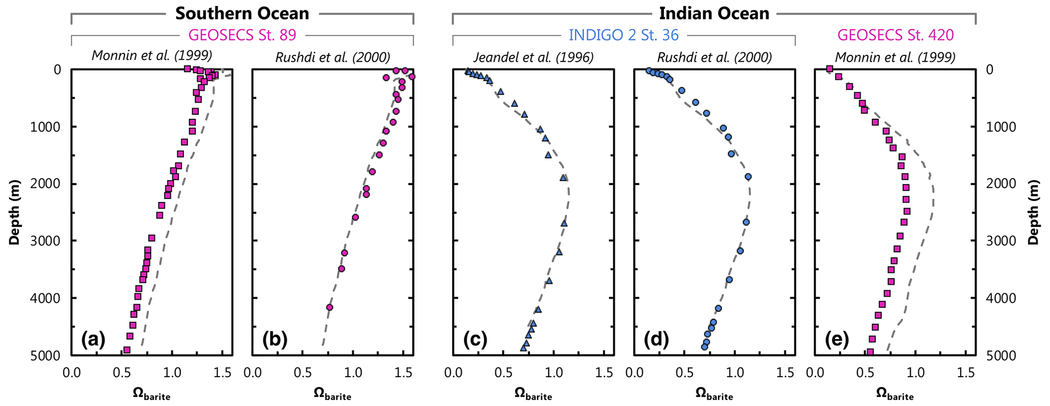
Figure A1Comparison of literature- (symbols) and model-3080-derived (dashed line) values of Ωbarite. Panels (a) and (b) show profiles of Ωbarite at GEOSECS st. 89 ( S, E). The other panels are from the Indian Ocean: (c) and (d) are from INDIGO 2 st. 36 ( S, E), and (e) is from GEOSECS st. 420 ( S, E), some ≈ 675 km north of INDIGO 2 st. 36.
We compare our model output with literature data Ωbarite at two locations in two basins (Fig. A1). These locations were chosen to ensure a fair comparison between studies; at each location, at least two studies calculated profiles of Ωbarite using the same underlying in situ data for [Ba], T, S, and pressure. Thus, any differences in modeled Ωbarite should derive from the thermodynamic model and not the input data. Likewise, literature profiles at these locations were based on calculations for pure, rather than strontian, BaSO4, as in our study. Published profiles of Ωbarite were extracted graphically from each study using WebPlotDigitizer (Rohatgi, 2022). This extraction process may introduce some minor scatter in the literature data, though this is relatively minor compared to the range of variation in Ωbarite.
First, we examine profiles of Ωbarite reported for GEOSECS st. 89 in the Southern Ocean (Fig. A1; Monnin et al., 1999; Rushdi et al., 2000). Modeled and published profiles show supersaturation in the surface ocean and undersaturation below 2000–2500 m. Profiles from Rushdi et al. (2000) show excellent agreement with Ωbarite calculated from model no. 3080 [Ba] and WOA T, S, and pressure, with our output offset by an MAE of 0.06 (n=22). Given that we use the same thermodynamic model as Rushdi et al. (2000), the overall excellent agreement with their study is not surprising. However, the result is nonetheless reassuring since our study uses mean annual values for the various inputs, whereas Rushdi et al. (2000) utilized in situ data. There is a slightly larger offset between our profile of Ωbarite and that calculated by Monnin et al. (1999), with our respective profile exhibiting an MAE of 0.13 (n=41). This most likely reflects differences in the underlying thermodynamic model and not the in situ data since our model reproduces the same overall profile shape as Monnin et al. (1999). Likewise, both Monnin et al. (1999) and Rushdi et al. (2000) used the same in situ input data, and their results are highly comparable, albeit with an offset similar to that between our results and Monnin et al. (1999).
Next we examine profiles of Ωbarite in the Indian Ocean for samples from INDIGO 2 st. 36 (Fig. A1; Jeandel et al., 1996; Rushdi et al., 2000). Profiles of Ωbarite show undersaturation at the surface, moderate supersaturation between 2000–3500 m, and then a return to undersaturated conditions down to the seafloor. Our profile shows overall excellent agreement with that of Jeandel et al. (1996), whereby a comparison of Ωbarite yields an MAE of 0.03 (n=21). Our profile shows similarly good agreement with Rushdi et al. (2000), whereby a comparison between our respective values of Ωbarite yields an MAE of 0.04 (n=20).
We also compared our results with data from st. 420 of GEOSECS (Monnin et al., 1999), which is located ≈ 675 km north of INDIGO 2 st. 36 (Fig. 2). As with data from the Southern Ocean (GEOSECS St. 89), our profile data are offset to higher Ωbarite than those of Monnin et al. (1999), with slightly larger MAE of 0.16 (n=29). However, our modeled Ωbarite is generally in much closer agreement with Monnin et al. (1999) above 1100 m compared to below, equivalent to an MAE of 0.04 (n=8) and 0.21 (n=21), respectively. In this case it is more challenging to ascribe a unique cause to the differences in calculated Ωbarite; these offsets could relate to differences in the predictors or the thermodynamic model.
We can use these comparisons to estimate the prediction uncertainty of our model-derived values of Ωbarite. The MAE of the 133 comparisons shown in Fig. A1 yields a value of 0.10. However, there are different numbers of points in each profile; we thus believe it is more appropriate to average the MAE calculated for each of the five profiles, which yields a value of 0.08. Both values are similar to the 10 % prediction uncertainty reported by Monnin et al. (1999).
Overall, our ML-derived profiles of Ωbarite show excellent agreement with in situ data, both in terms of profile shape and values of Ωbarite. We use this comparison to estimate the prediction uncertainty of ML-derived values of Ωbarite, which we calculate as being between 0.08 and 0.10. Should a revised thermodynamic model and/or improved BaSO4 solubility coefficients become available, a new grid of Ωbarite could be calculated using model no. 3080 [Ba] and WOA T, S, and pressure data.
The supplement related to this article is available online at: https://doi.org/10.5194/essd-15-4023-2023-supplement.
Project conceptualization and funding acquisition were conducted by TJH. Data curation, formal analysis, investigation, and methodology were the responsibilities of OZM, AVS, HHK, AGD, and TJH. Data visualization was performed by AVS and TJH. Software was provided by OZM, AVS, and HHK. Writing (original draft) was conducted by OZM and TJH; review and editing of the paper were conducted by AVS, HHK, AGD, LMW, AMS, MG, and WDL.
The contact authors have declared that none of the authors has any competing interests.
Publisher's note: Copernicus Publications remains neutral with regard to jurisdictional claims in published maps and institutional affiliations.
We are grateful to the many data originators who contributed dissolved Ba data to the 2021 GEOTRACES Intermediate Data Product, as well as the funding agencies that made those contributions possible. The GEOTRACES IDP represents an international collaboration and is endorsed by the Scientific Committee on Oceanic Research. We are especially grateful to Frank Dehairs, who provided comments on an early draft of the text and shared additional testing data from the Indian Ocean, as well as Karen Grissom, who provided laboratory assistance to Alan M. Shiller. We kindly acknowledge the use of the Discovery high-performance compute nodes at Dartmouth College Research Computing. We are grateful to the editor, Christophe Monnin, Frank Pavia, and two anonymous reviewers, who provided insightful and constructive comments that helped us improve the paper.
Öykü Z. Mete was supported by WHOI's Academic Programs Office through a summer student fellowship. Alan M. Shiller was supported by the US National Science Foundation (grant nos. OCE-0927951, OCE-1137851, OCE-1261214, OCE-1436312, and OCE-1737024), as does Tristan J. Horner (grant nos. OCE-1736949, OCE-2023456, and OCE-2048604). Tristan J. Horner was further supported by the Andrew W. Mellon Foundation Endowed Fund for Innovative Research and the Breene M. Kerr Early Career Scientist Endowment Fund.
This paper was edited by Xingchen (Tony) Wang and reviewed by Christophe Monnin, Frank Pavia, and two anonymous referees.
Anagnostou, E., Sherrell, R. M., Gagnon, A., LaVigne, M., Field, M. P., and McDonough, W. F.: Seawater nutrient and carbonate ion concentrations recorded as P/Ca, Ba/Ca, and U/Ca in the deep-sea coral Desmophyllum dianthus, Geochim. Cosmochim. Ac., 75, 2529–2543, https://doi.org/10.1016/j.gca.2011.02.019, 2011.
Anscombe, F. J.: Graphs in Statistical Analysis, Am. Stat., 27, 17–21, https://doi.org/10.1080/00031305.1973.10478966, 1973.
Baars, O., Abouchami, W., Galer, S. J., Boye, M., and Croot, P. L.: Dissolved cadmium in the Southern Ocean: Distribution, speciation, and relation to phosphate, Limnol. Oceanogr., 59, 385–399, https://doi.org/10.4319/lo.2014.59.2.0385, 2014.
Bains, S., Norris, R. D., Corfield, R. M., and Faul, K. L.: Termination of global warmth at the Palaeocene/Eocene boundary through productivity feedback, Nature, 407, 171–174, https://doi.org/10.1038/35025035, 2000.
Bates, S. L., Hendry, K. R., Pryer, H. V., Kinsley, C. W., Pyle, K. M., Woodward, E. M. S., and Horner, T. J.: Barium isotopes reveal the role of ocean circulation on barium cycling in the Atlantic, Geochim. Cosmochim. Ac., 204, 286–299, https://doi.org/10.1016/j.gca.2017.01.043, 2017.
Boyer, T. P., García, H. E., Locarnini, R. A., Zweng, M. M., Mishonov, A. V., Reagan, J. R., Weathers, K. A., Baranova, O. K., Paver, C. R., Seidov, D., and Smolyar, I. V.: World Ocean Atlas 2018, NOAA National Centers for Environmental Information [data set], https://www.ncei.noaa.gov/archive/accession/NCEI-WOA18 (last access: 4 September 2023), 2018.
Bishop, J. K.: The barite–opal–organic carbon association in oceanic particulate matter, Nature, 332, 341–343, https://doi.org/10.1038/332341a0, 1988.
Bishop, J. K. B.: Regional extremes in particulate matter composition and flux: Effects on the chemistry of the ocean interior, in: Productivity of the Ocean. Present and Past, edited by: Berger, W. H., Smetacek, V. S., and Wefer, G., Wiley, 117–137, ISBN-10 0471922463, 1989.
Blount, C. W.: Barite solubilities and thermodynamic quantities up to 300 degrees C and 1400 bars, Am. Mineral., 62, 942–957, 1977.
Boyer, T. P., García, H. E., Locarnini, R. A., Zweng, M. M., Mishonov, A. V., Reagan, J. R., Weathers, K. A.,Baranova, O. K., Paver, C. R., Seidov, D., and Smolyar, I. V.: World Ocean Atlas 2018, NOAA National Centers for Environmental Information, [data set], https://www.ncei.noaa.gov/archive/accession/NCEI-WOA18 (last access: 4 September 2023), 2018.
Boyle, E. and Edmond, J. M.: Copper in surface waters south of New Zealand, Nature, 253, 107–109, https://doi.org/10.1038/253107a0, 1975.
Bridgestock, L., Hsieh, Y.-T., Porcelli, D., Homoky, W. B., Bryan, A., and Henderson, G. M.: Controls on the barium isotope compositions of marine sediments, Earth Planet. Sc. Lett., 481, 101–110, https://doi.org/10.1016/j.epsl.2017.10.019, 2018.
Cao, Z., Li, Y., Rao, X., Yu, Y., Hathorne, E. C., Siebert, C., Dai, M., and Frank, M.: Constraining barium isotope fractionation in the upper water column of the South China Sea, Geochim. Cosmochim. Ac., 288, 120–137, https://doi.org/10.1016/j.gca.2020.08.008, 2020.
Cao, Z., Rao, X., Yu, Y., Siebert, C., Hathorne, E. C., Liu, B., Wang, G., Lian, E., Wang, Z., Zhang, R., Gao, L., Wei, G., Yang, S., Dai, M., and Frank, M.: Stable barium isotope dynamics during estuarine mixing, Geophys. Res. Lett., 48, e2021GL095680, https://doi.org/10.1029/2021GL095680, 2021.
Carter, S. C., Paytan, A., and Griffith, E. M.: Toward an Improved Understanding of the Marine Barium Cycle and the Application of Marine Barite as a Paleoproductivity Proxy, Minerals, 10, 421, https://doi.org/10.3390/min10050421, 2020.
Chan, L. H., Drummond, D., Edmond, J. M., and Grant, B.: On the barium data from the Atlantic GEOSECS expedition, Deep-Sea Res., 24, 613–649, https://doi.org/10.1016/0146-6291(77)90505-7, 1977.
Charbonnier, Q., Bouchez, J., Gaillardet, J., and Gayer, É.: Barium stable isotopes as a fingerprint of biological cycling in the Amazon River basin, Biogeosciences, 17, 5989–6015, https://doi.org/10.5194/bg-17-5989-2020, 2020.
Chow, T. J. and Goldberg, E. D.: On the marine geochemistry of barium, Geochim. Cosmochim. Ac., 20, 192–198, https://doi.org/10.1016/0016-7037(60)90073-9, 1960.
Coffey, M., Dehairs, F., Collette, O., Luther, G., Church, T., and Jickells, T.: The Behaviour of Dissolved Barium in Estuaries, Estuar. Coast. Shelf S., 45, 113–121, https://doi.org/10.1006/ecss.1996.0157, 1997.
Copernicus Marine Environment Monitoring Service: Global Ocean Chlorophyll, PP and PFT (Copernicus-GlobColour) from Satellite Observations: Monthly and Daily Interpolated (Reprocessed from 1997), Mercator Ocean International [data set], https://doi.org/10.48670/MOI-00100, 2021.
Craig, H. and Turekian, K. K.: The GEOSECS program: 1976–1979, Earth Planet. Sc. Lett., 49, 263–265, https://doi.org/10.1016/0012-821X(76)90062-5, 1980.
Crameri, F.: Scientific colour maps, Zenodo [code], https://doi.org/10.5281/zenodo.5501399, 2018.
Cressie, N. A. C.: Spatial Prediction and Kriging, in: Statistics for Spatial Data, 105–209, https://doi.org/10.1002/9781119115151.ch3, 1993.
Cutter, G. A.: Intercalibration in chemical oceanography – getting the right number, Limnol. Oceanogr.-Meth., 11, 418–424, https://doi.org/10.4319/lom.2013.11.418, 2013.
Dehairs, F., Chesselet, R., and Jedwab, J.: Discrete suspended particles of barite and the barium cycle in the open ocean, Earth Planet. Sc. Lett., 49, 528–550, https://doi.org/10.1016/0012-821X(80)90094-1, 1980.
DeVries, T.: The oceanic anthropogenic CO2 sink: Storage, air-sea fluxes, and transports over the industrial era, Global Biogeochem. Cy., 28, 631–647, https://doi.org/10.1002/2013GB004739, 2014.
Dickens, G. R., Fewless, T., Thomas, E., and Bralower, T. J.: Excess barite accumulation during the Paleocene-Eocene thermal Maximum: Massive input of dissolved barium from seafloor gas hydrate reservoirs, in: Causes and consequences of globally warm climates in the early Paleogene, edited by: Wing, S. L., Gingerich, P. D., Schmitz, B., and Thomas, E., Geological Society of America, https://doi.org/10.1130/0-8137-2369-8.11, 2003.
Dymond, J., Suess, E., and Lyle, M.: Barium in Deep-Sea Sediment: A Geochemical Proxy for Paleoproductivity, Paleoceanography, 7, 163–181, https://doi.org/10.1029/92PA00181, 1992.
Eagle, M., Paytan, A., Arrigo, K. R., van Dijken, G., and Murray, R. W.: A comparison between excess barium and barite as indicators of carbon export, Paleoceanography, 18, 1021, https://doi.org/10.1029/2002PA000793, 2003.
Eakins, B. W. and Sharman, G. F.: Volumes of the World's Oceans from ETOPO1, NOAA National Geophysical Data Center [data set], Boulder, CO, https://www.ngdc.noaa.gov/mgg/global/etopo1_ocean_volumes.html (last access: 4 September 2023), 2010.
Edmond, J. M., Boyle, E. D., Drummond, D., Grant, B., and Mislick, T.: Desorption of barium in the plume of the Zaire (Congo) River, Neth. J. Sea Res., 12, 324–328, https://doi.org/10.1016/0077-7579(78)90034-0, 1978.
Esser, B. K. and Volpe, A. M.: At-sea high-resolution chemical mapping: Extreme barium depletion in North Pacific surface water, Mar. Chem., 79, 67–79, https://doi.org/10.1016/S0304-4203(02)00037-3, 2002.
García, H. E., Weathers, K. W., Paver, C. R., Smolyar, I., Boyer, T. P., Locarnini, R. A., Zweng, M. M., Mishonov, A. V., Baranova, O. K., Seidov, D., and Reagan, J. R.: World Ocean Atlas 2018, Volume 3: Dissolved Oxygen, Apparent Oxygen Utilization, and Dissolved Oxygen Saturation, edited by: Mishonov, A., NOAA Atlas NESDIS 83 [data set], 38 pp., http://www.nodc.noaa.gov/OC5/indprod.html (last access: 4 September 2023), 2018a.
García, H. E., Weathers, K. W., Paver, C. R., Smolyar, I., Boyer, T. P., Locarnini, R. A., Zweng, M. M., Mishonov, A. V., Baranova, O. K., Seidov, D., and Reagan, J. R.: World Ocean Atlas 2018, Vol. 4: Dissolved Inorganic Nutrients (phosphate, nitrate and nitrate+nitrite, silicate), edited by: Mishonov, A., NOAA Atlas NESDIS 84 [data set], 35 pp., http://www.nodc.noaa.gov/OC5/indprod.html (last access: 4 September 2023), 2018b.
GEOTRACES Intermediate Data Product Group: The GEOTRACES Intermediate Data Product 2021 (IDP2021), NERC EDS British Oceanographic Data Centre NOC [data set], https://doi.org/10.5285/cf2d9ba9-d51d-3b7c-e053-8486abc0f5fd, 2021.
Glover, D., Jenkins, W., and Doney, S.: Modeling Methods for Marine Science, Cambridge University Press, https://doi.org/10.1017/CBO9780511975721, 2011.
Gonneea, M. E., Cohen, A. L., DeCarlo, T. M., and Charette, M. A.: Relationship between water and aragonite barium concentrations in aquaria reared juvenile corals, Geochim. Cosmochim. Ac., 209, 123–134, https://doi.org/10.1016/j.gca.2017.04.006, 2017.
Gruber, N. and Sarmiento, J. L.: Global patterns of marine nitrogen fixation and denitrification, Global Biogeochem. Cy., 11, 235–266, https://doi.org/10.1029/97GB00077, 1997.
Guay, C. K. and Falkner, K. K.: A survey of dissolved barium in the estuaries of major Arctic rivers and adjacent seas, Cont. Shelf Res., 18, 859–882, https://doi.org/10.1016/S0278-4343(98)00023-5, 1998.
Hathorne, E. C., Gagnon, A., Felis, T., Adkins, J., Asami, R., Boer, W., Caillon, N., Case, D., Cobb, K. M., Douville, E., deMenocal, P., Eisenhauer, A., Garbe-Schönberg, D., Geibert, W., Goldstein, S., Hughen, K., Inoue, M., Kawahata, H., Kölling, M., Cornec, F. L., Linsley, B. K., McGregor, H. V., Montagna, P., Nurhati, I. S., Quinn, T. M., Raddatz, J., Rebaubier, H., Robinson, L., Sadekov, A., Sherrell, R., Sinclair, D., Tudhope, A. W., Wei, G., Wong, H., Wu, H. C., and You, C.-F.: Interlaboratory study for coral Sr/Ca and other element/Ca ratio measurements, Geochem. Geophys. Geosy., 14, 3730–3750, https://doi.org/10.1002/ggge.20230, 2013.
Hayes, C. T., Anderson, R. F., Cheng, H., Conway, T. M., Edwards, R. L., Fleisher, M. Q., Ho, P., Huang, K.-F., John, S. G., Landing, W. M., Little, S. H., Lu, Y., Morton, P. L., Moran, S. B., Robinson, L. F., Shelley, R. U., Shiller, A. M., and Zheng, X.-Y.: Replacement Times of a Spectrum of Elements in the North Atlantic Based on Thorium Supply, Global Biogeochem. Cy., 32, 1294–1311, https://doi.org/10.1029/2017GB005839, 2018.
Hayes, C. T., Costa, K. M., Anderson, R. F., Calvo, E., Chase, Z., Demina, L. L., Dutay, J.-C., German, C. R., Heimbürger-Boavida, L.-E., Jaccard, S. L., Jacobel, A., Kohfeld, K. E., Kravchishina, M. D., Lippold, J., Mekik, F., Missiaen, L., Pavia, F. J., Paytan, A., Pedrosa-Pamies, R., Petrova, M. V., Rahman, S., Robinson, L. F., Roy-Barman, M., Sanchez-Vidal, A., Shiller, A., Tagliabue, A., Tessin, A. C., van Hulten, M., and Zhang, J.: Global Ocean Sediment Composition and Burial Flux in the Deep Sea, Global Biogeochem. Cy., 35, e2020GB006769, https://doi.org/10.1029/2020GB006769, 2021.
Holte, J., Talley, L. D., Gilson, J., and Roemmich, D.: An Argo mixed layer climatology and database, Geophys. Res. Lett., 44, 5618–5626, https://doi.org/10.1002/2017GL073426, 2017.
Holzer, M., Primeau, F. W., DeVries, T., and Matear, R.: The Southern Ocean silicon trap: Data-constrained estimates of regenerated silicic acid, trapping efficiencies, and global transport paths, J. Geophys. Res.-Oceans, 119, 313–331, https://doi.org/10.1002/2013JC009356, 2014.
Hood, E. M., Sabine, C. L., and Sloyan, B. M. (Eds.): The GO-SHIP Repeat Hydrography Manual: A Collection of Expert Reports and Guidelines, IOCCP Report Number 14, ICPO Publication Series Number 134, http://www.go-ship.org/HydroMan.html (last access: 4 September 2023), 2010.
Hönisch, B., Allen, K. A., Russell, A. D., Eggins, S. M., Bijma, J., Spero, H. J., Lea, D. W., and Yu, J.: Planktic foraminifers as recorders of seawater Ba/Ca, Mar. Micropaleontol., 79, 52–57, https://doi.org/10.1016/j.marmicro.2011.01.003, 2011.
Hoppema, M., Dehairs, F., Navez, J., Monnin, C., Jeandel, C., Fahrbach, E., and de Baar, H. J. W.: Distribution of barium in the Weddell Gyre: Impact of circulation and biogeochemical processes, Mar. Chem., 122, 118–129, https://doi.org/10.1016/j.marchem.2010.07.005, 2010.
Horner, T. J. and Crockford, P. W.: Barium Isotopes: Drivers, Dependencies, and Distributions through Space and Time, 1st Edn., Cambridge University Press, https://doi.org/10.1017/9781108865845, 2021.
Horner, T. J. and Mete, O. Z.: A spatially and vertically resolved global grid of dissolved barium concentrations in seawater determined using Gaussian Process Regression machine learning, Version 2, Biological and Chemical Oceanography Data Management Office (BCO-DMO) [data set], https://doi.org/10.26008/1912/bco-dmo.885506.2, 2023.
Horner, T. J., Kinsley, C. W., and Nielsen, S. G.: Barium-isotopic fractionation in seawater mediated by barite cycling and oceanic circulation, Earth Planet. Sc. Lett., 430, 511–522, https://doi.org/10.1016/j.epsl.2015.07.027, 2015.
Hsieh, Y.-T. and Henderson, G. M.: Barium stable isotopes in the global ocean: Tracer of Ba inputs and utilization, Earth Planet. Sc. Lett., 473, 269–278, https://doi.org/10.1016/j.epsl.2017.06.024, 2017.
Jacquet, S. H. M., Dehairs, F., and Rintoul, S.: A high-resolution transect of dissolved barium in the Southern Ocean, Geophys. Res. Lett., 31, L14301, https://doi.org/10.1029/2004GL020016, 2004.
Jeandel, C., Dupré, B., Lebaron, G., Monnin, C., and Minster, J.-F.: Longitudinal distributions of dissolved barium, silica and alkalinity in the western and southern Indian Ocean, Deep-Sea Res. Pt. I, 43, 1–31, https://doi.org/10.1016/0967-0637(95)00098-4, 1996.
John, S. G., Liang, H., Weber, T., DeVries, T., Primeau, F., Moore, K., Holzer, M., Mahowald, N., Gardner, W., Mishonov, A., Richardson, M. J., Faugere, Y., and Taburet, G.: AWESOME OCIM: A simple, flexible, and powerful tool for modeling elemental cycling in the oceans, Chem. Geol., 533, 119403, https://doi.org/10.1016/j.chemgeo.2019.119403, 2020.
Joung, D. and Shiller, A. M.: Dissolved barium behavior in Louisiana Shelf waters affected by the Mississippi/Atchafalaya River mixing zone, Geochim. Cosmochim. Ac., 141, 303–313, https://doi.org/10.1016/j.gca.2014.06.021, 2014.
Jullion, L., Jacquet, S. H. M., and Tanhua, T.: Untangling biogeochemical processes from the impact of ocean circulation: First insight on the Mediterranean dissolved barium dynamics, Global Biogeochem. Cy., 31, 1256–1270, https://doi.org/10.1002/2016GB005489, 2017.
Kawabe, M. and Fujio, S.: Pacific Ocean circulation based on observation, J. Oceanogr., 66, 389–403, https://doi.org/10.1007/s10872-010-0034-8, 2010.
Komagoe, T., Watanabe, T., Shirai, K., Yamazaki, A., and Uematu, M.: Geochemical and Microstructural Signals in Giant Clam Tridacna Maxima Recorded Typhoon Events at Okinotori Island, Japan, J. Geophys. Res.-Biogeo., 123, 1460–1474, https://doi.org/10.1029/2017JG004082, 2018.
LaVigne, M., Hill, T. M., Spero, H. J., and Guilderson, T. P.: Bamboo coral Ba/Ca: Calibration of a new deep ocean refractory nutrient proxy, Earth Planet. Sc. Lett., 312, 506–515, https://doi.org/10.1016/j.epsl.2011.10.013, 2011.
LaVigne, M., Grottoli, A. G., Palardy, J. E., and Sherrell, R. M.: Multi-colony calibrations of coral Ba/Ca with a contemporaneous in situ seawater barium record, Geochim. Cosmochim. Ac., 179, 203–216, https://doi.org/10.1016/j.gca.2015.12.038, 2016.
Lea, D. W. and Boyle, E. A.: Foraminiferal reconstruction of barium distributions in water masses of the glacial oceans, Paleoceanography, 5, 719–742, https://doi.org/10.1029/PA005i005p00719, 1990.
Lea, D. W., Shen, G. T., and Boyle, E. A.: Coralline barium records temporal variability in equatorial Pacific upwelling, Nature, 340, 373–376, https://doi.org/10.1038/340373a0, 1989.
Le Roy, E., Sanial, V., Charette, M. A., van Beek, P., Lacan, F., Jacquet, S. H. M., Henderson, P. B., Souhaut, M., García-Ibáñez, M. I., Jeandel, C., Pérez, F. F., and Sarthou, G.: The 226Ra–Ba relationship in the North Atlantic during GEOTRACES-GA01, Biogeosciences, 15, 3027–3048, https://doi.org/10.5194/bg-15-3027-2018, 2018.
Light, T. and Norris, R.: Quantitative visual analysis of marine barite microcrystals: Insights into precipitation and dissolution dynamics, Limnol. Oceanogr., 66, 3619–3629, https://doi.org/10.1002/lno.11902, 2021.
Locarnini, R. A., Mishonov, A. V., Baranova, O. K., Boyer, T. P., Zweng, M. M., Garcia, H. E., Reagan, J. R., Seidov, D., Weathers, K. W., Paver, C. R., and Smolyar, I. V.: World Ocean Atlas 2018, Volume 1: Temperature, NOAA Atlas NESDIS 81 [data set], 52 pp., https://www.nodc.noaa.gov/OC5/indprod.html (last access: 4 September 2023), 2018.
Monnin, C., Jeandel, C., Cattaldo, T., and Dehairs, F.: The marine barite saturation state of the world's oceans, Mar. Chem., 65, 253–261, https://doi.org/10.1016/S0304-4203(99)00016-X, 1999.
National Geophysical Data Center: 5-minute Gridded Global Relief Data (ETOPO5), NOAA National Geophysical Data Center [data set], https://doi.org/10.7289/V5D798BF, 1993.
Orsi, A. H., Whitworth III, T., and Nowlin Jr., W. D.: On the meridional extent and fronts of the Antarctic Circumpolar Current, Deep-Sea Res. Pt. I, 42, 641–673, https://doi.org/10.1016/0967-0637(95)00021-W, 1995.
Paytan, A. and Griffith, E. M.: Marine barite: Recorder of variations in ocean export productivity, Deep-Sea Res. Pt. II, 54, 687–705, https://doi.org/10.1016/j.dsr2.2007.01.007, 2007.
Paytan, A. and Kastner, M.: Benthic Ba fluxes in the central Equatorial Pacific, implications for the oceanic Ba cycle, Earth Planet. Sc. Lett., 142, 439–450, https://doi.org/10.1016/0012-821X(96)00120-3, 1996.
Pyle, K. M., Hendry, K. R., Sherrell, R. M., Legge, O., Hind, A. J., Bakker, D., Venables, H., and Meredith, M. P.: Oceanic fronts control the distribution of dissolved barium in the Southern Ocean, Mar. Chem., 204, 95–106, https://doi.org/10.1016/j.marchem.2018.07.002, 2018.
Rafter, P. A., Bagnell, A., Marconi, D., and DeVries, T.: Global trends in marine nitrate N isotopes from observations and a neural network-based climatology, Biogeosciences, 16, 2617–2633, https://doi.org/10.5194/bg-16-2617-2019, 2019.
Rahman, S., Shiller, A. M., Anderson, R. F., Charette, M. A., Hayes, C. T., Gilbert, M., Grissom, K. R., Lam, P. J., Ohnemus, D. C., Pavia, F. J., Twining, B. S., and Vivancos, S. M.: Dissolved and particulate barium distributions along the US GEOTRACES North Atlantic and East Pacific Zonal Transects (GA03 and GP16): Global implications for the marine barium cycle, Global Biogeochem. Cy., 36, e2022GB007330, https://doi.org/10.1029/2022GB007330, 2022.
Raju, K. and Atkinson, G.: Thermodynamics of “scale” mineral solubilities. 1. Barium sulfate(s) in water and aqueous sodium chloride, J. Chem. Eng. Data, 33, 490–495, https://doi.org/10.1021/je00054a029, 1988.
Rasmussen, C. E. and Williams, C. K. I.: Gaussian processes for machine learning, MIT Press, https://doi.org/10.7551/mitpress/3206.001.0001, 2006.
Roeske, T., van der Loeff, M. R., Middag, R., and Bakker, K.: Deep water circulation and composition in the Arctic Ocean by dissolved barium, aluminium and silicate, Mar. Chem., 132–133, 56–67, https://doi.org/10.1016/j.marchem.2012.02.001, 2012.
Rohatgi, A.: WebPlotDigitizer, Version: 4.6, Pacifica, CA, USA, https://automeris.io/WebPlotDigitizer (last access: 4 September 2023), 2022.
Roshan, S. and DeVries, T.: Global Contrasts Between Oceanic Cycling of Cadmium and Phosphate, Global Biogeochem. Cy., 35, e2021GB006952, https://doi.org/10.1029/2021GB006952, 2021.
Roshan, S., DeVries, T., Wu, J., and Chen, G.: The internal cycling of zinc in the ocean, Global Biogeochem. Cy., 32, 1833–1849, https://doi.org/10.1029/2018GB006045, 2018.
Roshan, S., DeVries, T., and Wu, J.: Constraining the global ocean Cu cycle with a data-assimilated diagnostic model, Global Biogeochem. Cy., 34, e2020GB006741, https://doi.org/10.1029/2020GB006741, 2020.
Rushdi, A. I., McManus, J., and Collier, R. W.: Marine barite and celestite saturation in seawater, Mar. Chem., 69, 19–31, https://doi.org/10.1016/S0304-4203(99)00089-4, 2000.
Samanta, S. and Dalai, T. K.: Dissolved and particulate Barium in the Ganga (Hooghly) River estuary, India: Solute-particle interactions and the enhanced dissolved flux to the oceans, Geochim. Cosmochim. Ac., 195, 1–28, https://doi.org/10.1016/j.gca.2016.09.005, 2016.
Sarmiento, J. L., Gruber, N., Brzezinski, M. A., and Dunne, J. P.: High-latitude controls of thermocline nutrients and low latitude biological productivity, Nature, 427, 56–60, https://doi.org/10.1038/nature02127, 2004.
Schenau, S. J., Prins, M. A., De Lange, G. J., and Monnin, C.: Barium accumulation in the Arabian Sea: Controls on barite preservation in marine sediments, Geochim. Cosmochim. Ac., 65, 1545–1556, https://doi.org/10.1016/S0016-7037(01)00547-6, 2001.
Schlitzer, R.: Ocean Data View, https://odv.awi.de (last access: 4 September 2023), 2023.
Schlitzer, R., Anderson, R. F., Dodas, E. M., Lohan, M., Geibert, W., Tagliabue, A., Bowie, A., Jeandel, C., Maldonado, M. T., Landing, W. M., Cockwell, D., Abadie, C., Abouchami, W., Achterberg, E. P., Agather, A., Aguliar-Islas, A., van Aken, H. M., Andersen, M., Archer, C., Auro M., de Baar, H. J., Baars, O., Baker, A. R., Bakker, K., Basak, C., Baskaran, M., Bates, N. R., Bauch, D., van Beek, P., Behrens, M. K., Black, E., Bluhm, K., Bopp, L., Bouman, H., Bowman, K., Bown, J., Boyd, P., Boye, M., Boyle, E. A., Branellec, P., Bridgestock, L., Brissebrat, G., Browning, T., Bruland, K. W., Brumsack, H. J., Brzezinski, M., Buck, C. S., Buck, K. N., Buesseler, K., Bull, A., Butler, E., Cai, P., Mor, P. C., Cardinal, D., Carlson, C., Carrasco, G., Casacuberta, N., Casciotti, K. L., Castrillejo, M., Chamizo, E., Chance, R., Charette, M. A., Chaves, J. E., Cheng, H., Chever, F., Christl, M., Church, T. M., Closset, I., Colman, A., Conway, T. M., Cossa, D., Croot, P., Cullen, J. T., Cutter, G. A., Daniels, C., Dehairs, F., Deng, F., Dieu, H. T., Duggan, B., Dulaquais, G., Dumousseaud, C., EchegoyenSanz, Y., Edwards, R. L., Ellwood, M., Fahrbach, E., Fitzsimmons, J. N., Flegal, A. R., Fleisher, M. Q., van de Flierdt, T., Frank, M., Friedrich, J., Fripiat, F., Fröllje, H., Galer, S. J. G., Gamo, T., Ganeshram, R. S., GarciaOrellana, J., GarciaSolsona, E., GaultRingold, M., George, E., Gerringa, L. J. A., Gilbert, M., Godoy, J. M., Goldstein, S. L., Gonzalez, S. R., Grissom, K., Hammerschmidt, C., Hartman, A., Hassler, C. S., Hathorne, E. C., Hatta, M., Hawco, N., Hayes, C. T., Heimbürger, L. E., Helgoe, J., Heller, M., Henderson, G. M., Henderson, P. B., van Heuven, S., Ho, P., Horner, T. J., Hsieh, Y. T., Huang, K. F., Humphreys, M. P., Isshiki, K., Jacquot, J. E., Janssen, D. J., Jenkins, W. J., John, S., Jones, E. M., Jones, J. L., Kadko, D. C., Kayser, R., Kenna, T. C., Khondoker, R., Kim, T., Kipp, L., Klar, J. K., Klunder, M., Kretschmer, S., Kumamoto, Y., Laan, P., Labatut, M., Lacan, F., Lam, P. J., Lambelet, M., Lamborg, C. H., Le Moigne, F. A. C., Le Roy, E., Lechtenfeld, O. J., Lee, J. M., Lherminier, P., Little, S., LópezLora, M., Lü, Y., Masqué, P., Mawji, E., McClain, C. R., Measures, C., Mehic, S., Barraqueta, J. L. M., van der Merwe, P., Middag, R., Mieruch, S., Milne, A., Minami, T., Moffett, J. W., Moncoiffe, G., Moore, W. S., Morris, P. J., Morton, P. L., Nakaguchi, Y., Nakayama, N., Niedermiller, J., Nishioka, J., Nishiuchi, A., Noble, A., Obata, H., Ober, S., Ohnemus, D. C., van Ooijen, J., OSullivan, J., Owens, S., Pahnke, K., Paul, M., Pavia, F., Pena, L. D., Peters, B., Planchon, F., Planquette, H., Pradoux, C., Puigcorbe, V., Quay, P., Queroue, F., Radic, A., Rauschenberg, S., Rehkämper, M., Rember, R., Remenyi, T., Resing, J. A., Rickli, J., Rigaud, S., Rijkenberg, M. J. A., Rintoul, S., Robinson, L. F., Roca-Martí, M., Rodellas, V., Roeske, T., Rolison, J. M., Rosenberg, M., Roshan, S., van der Loeff, M. M. R., Ryabenko, E., Saito, M. A., Salt, L. A., Sanial, V., Sarthou, G., Schallenberg, C., Schauer, U., Scher, H., Schlosser, C., Schnetger, B., Scott, P., Sedwick, P. N., Semiletov, I., Shelley, R., Sherrell, R. M., Shiller, A. M., Sigman, D. M., Singh, S. K., Slagter, H. A., Slater, E., Smethie, W. M., Snaith, H., Sohrin, Y., Sohst, B., Sonke, J. E., Speich, S., Steinfeldt, R., Stewart, G., Stichel, T., Stirling, C. H., Stutsman, J., Swarr, G. J., Swift, J. H., Thomas, A., Thorne, K., Till, C. P., Till, R., Townsend, A. T., Townsend, E., Tuerena, R., Twining, B. S., Vance, D., Velazquez, S., Venchiarutti, C., VillaAlfageme, M., Vivancos, S. M., Voelker, A. H. L., Wake, B., Warner, M. J., Watson, R., van Weerlee, E., Weigand, M. A., Weinstein, Y., Weiss, D., Wisotzki, A., Woodward, E. M. S., Wu, J., Wu, Y., Wuttig, K., Wyatt, N., Xiang, Y., Xie, R. C., Xue, Z., Yoshikawa, H., Zhang, J., Zhang, P., Zhao, Y., Zheng, L., Zheng, X. Y., Zieringer, M., Zimmer, L. A., Ziveri, P., Zunino, P., and Zurbrick, C.: The GEOTRACES Intermediate Data Product 2017, Chem. Geol., 493, 210–223, https://doi.org/10.1016/j.chemgeo.2018.05.040, 2018.
Schmitz, B.: Barium, equatorial high productivity, and the northward wandering of the Indian continent, Paleoceanogr., 2, 63–77, https://doi.org/10.1029/PA002i001p00063, 1987.
Schroeder, J. O., Murray, R. W., Leinen, M., Pflaum, R. C., and Janecek, T. R.: Barium in equatorial Pacific carbonate sediment: Terrigenous, oxide, and biogenic associations, Paleoceanogr., 12, 125–146, https://doi.org/10.1029/96PA02736, 1997.
Serno, S., Winckler, G., Anderson, R. F., Hayes, C. T., Ren, H., Gersonde, R., and Haug, G. H.: Using the natural spatial pattern of marine productivity in the Subarctic North Pacific to evaluate paleoproductivity proxies, Paleoceanogr., 29, 438–453, https://doi.org/10.1002/2013PA002594, 2014.
Sherwen, T., Chance, R. J., Tinel, L., Ellis, D., Evans, M. J., and Carpenter, L. J.: A machine-learning-based global sea-surface iodide distribution, Earth Syst. Sci. Data, 11, 1239–1262, https://doi.org/10.5194/essd-11-1239-2019, 2019.
Sinclair, D. J. and McCulloch, M. T.: Corals record low mobile barium concentrations in the Burdekin River during the 1974 flood: Evidence for limited Ba supply to rivers?, Palaeogeogr. Palaeoclim., 214, 155–174, https://doi.org/10.1016/j.palaeo.2004.07.028, 2004.
Singh, A. K., Marcantonio, F., and Lyle, M.: An assessment of xsBa flux as a paleoproductivity indicator and its water-depth dependence in the easternmost equatorial Pacific Ocean, Paleoceanography and Paleoclimatology, 35, e2020PA003945, https://doi.org/10.1029/2020PA003945, 2020.
Singh, S. P., Singh, S. K., and Bhushan, R.: Internal cycling of dissolved barium in water column of the Bay of Bengal, Mar. Chem., 154, 12–23, https://doi.org/10.1016/j.marchem.2013.04.013, 2013.
Stewart, J. A., Li, T., Spooner, P. T., Burke, A., Chen, T., Roberts, J., Rae, J. W. B., Peck, V., Kender, S., Liu, Q., and Robinson, L. F.: Productivity and Dissolved Oxygen Controls on the Southern Ocean Deep-Sea Benthos During the Antarctic Cold Reversal, Paleoceanography and Paleoclimatology, 36, e2021PA004288, https://doi.org/10.1029/2021PA004288, 2021.
Stroobants, N., Dehairs, F., Goeyens, L., Vanderheijden, N., and Van Grieken, R.: Barite formation in the Southern Ocean water column, Mar. Chem., 35, 411–421, https://doi.org/10.1016/S0304-4203(09)90033-0, 1991.
Talley, L. D.: An Okhotsk Sea water anomaly: implications for ventilation in the North Pacific, Deep-Sea Res. Pt. I, 38, S171–S190, https://doi.org/10.1016/S0198-0149(12)80009-4, 1991.
Talley, L. D.: Freshwater transport estimates and the global overturning circulation: Shallow, deep and throughflow components, Prog. Oceanogr., 78, 257–303, https://doi.org/10.1016/j.pocean.2008.05.001, 2008.
Talley, L. D., Pickard, G. L., and Emery, W. J. (Eds.): Descriptive physical oceanography: An introduction, 6th Edn., Academic Press, https://doi.org/10.1016/C2009-0-24322-4, 2011.
Whitmore, L. M., Shiller, A. M., Horner, T. J., Xiang, Y., Auro, M. E., Bauch, D., Dehairs, F., Lam, P. J., Li, J., Maldonado, M. T., Mears, C., Newton, R., Pasqualini, A., Planquette, H., Rember, R., and Thomas, H.: Strong Margin Influence on the Arctic Ocean Barium Cycle Revealed by Pan-Arctic Synthesis, J. Geophys. Res.-Oceans, 127, e2021JC017417, https://doi.org/10.1029/2021JC017417, 2022.
Wyatt, N. J., Milne, A., Woodward, E. M. S., Rees, A. P., Browning, T. J., Bouman, H. A., Worsfold, P. J., and Lohan, M. C.: Biogeochemical cycling of dissolved zinc along the GEOTRACES South Atlantic transect GA10 at 40 S, Global Biogeochem. Cy., 28, 44–56, https://doi.org/10.1002/2013GB004637, 2014.
Zhang, Z., Yu, Y., Hathorne, E. C., Vieira, L. H., Grasse, P., Siebert, C., Rahlf, P., and Frank, M.: Decoupling of Barium and Silicon at the Congo River-dominated Southeast Atlantic Margin: Insights from Combined Barium and Silicon Isotopes, Global Biogeochem. Cy., 37, e2022GB007610, https://doi.org/10.1029/2022GB007610, 2023.
Zweng, M. M., Reagan, J. R., Seidov, D., Boyer, T. P., Locarnini, R. A., Garcia, H. E., Mishonov, A. V., Baranova, O. K., Weathers, K. W., Paver, C. R., and Smolyar, I. V.: World Ocean Atlas 2018, Volume 2: Salinity, A. Mishonov, Tech. Ed., NOAA Atlas NESDIS 82 [data set], 50 pp., http://www.nodc.noaa.gov/OC5/indprod.html (last access: 4 September 2023), 2018.