the Creative Commons Attribution 4.0 License.
the Creative Commons Attribution 4.0 License.
 | 05 Jul 2023
Res-CN (Reservoir dataset in China): hydrometeorological time series and landscape attributes across 3254 Chinese reservoirs
Youjiang Shen
Karina Nielsen
Menaka Revel
Dedi Liu
Dai Yamazaki
Dams and reservoirs are human-made infrastructures that have attracted increasing attention because of their societal and environmental significance. Towards better management and conservation of reservoirs, a dataset of reservoir-catchment characteristics is needed, considering that the amount of water and material flowing into and out of reservoirs depends on their locations on the river network and the properties of the upstream catchment. To date, no dataset exists for reservoir-catchment characteristics. The aim of this study is to develop the first database featuring reservoir-catchment characteristics for 3254 reservoirs with storage capacity totaling 682 595 km3 (73.2 % of reservoir water storage capacity in China) to support the management and conservation of reservoirs in the context of catchment level. To ensure a more representative and accurate mapping of local variables of large reservoirs, reservoir catchments are delineated into full catchments (their full upstream contributing areas) and intermediate catchments (subtracting the area contributed by upstream reservoirs from the full upstream part of the current reservoir). Using both full catchments and intermediate catchments, characteristics of reservoir catchments were extracted, with a total of 512 attributes in six categories (i.e., reservoir and catchment body characteristics, topography, climate, soil and geology, land cover and use, and anthropogenic activity characteristics). Besides these static attributes, time series of 15 meteorological variables of catchments were extracted to support hydrological simulations for a better understanding of drivers of reservoir environment change. Moreover, we provide a comprehensive and extensive reservoir dataset on water level (data available for 20 % of 3254 reservoirs), water surface area (99 %), storage anomaly (92 %), and evaporation (98 %) from multisource satellites such as radar and laser altimeters and images from Landsat and Sentinel satellites. These products significantly enhance spatial and temporal coverage in comparison to existing similar products (e.g., 67 % increase in spatial resolution of water level and 225 % increase in storage anomaly) and contribute to our understanding of reservoir properties and functions within the Earth system by incorporated national or global hydrological modeling. In situ data of 138 reservoirs are employed in this study as a valuable reference for evaluation, thus enhancing our confidence in the data quality and enhancing our understanding of the accuracy of current satellite datasets. Along with its extensive attributes, the Reservoir dataset in China (Res-CN) can support a broad range of applications such as water resources, hydrologic/hydrodynamic modeling, and energy planning. Res-CN is on Zenodo through https://doi.org/10.5281/zenodo.7664489 (Shen et al., 2022c).
- Article
(15980 KB) - Full-text XML
-
Supplement
(5474 KB) - BibTeX
- EndNote


The role of reservoirs in the hydrological and biogeochemical cycles is closely tied to their characteristics of water surface area, water level, evaporation, and storage variation. In addition, the amount and rate of water and materials flowing into and out of reservoirs depend on their location in the river network, reservoir upstream catchment attributes (e.g., catchment size, topography, geology, soil, and land cover), and meteorological variables (e.g., precipitation and temperature). An explicit spatial knowledge of all these characteristics (see Fig. A1) is crucial for determining surface water availability and modulating water flux interactions among various Earth system components, including terrestrial water storage dynamics (Busker et al., 2019; Chaudhari et al., 2018); terrestrial carbon cycle (Marx et al., 2017); geochemical cycle (Maavara et al., 2020); surface energy budget (Buccola et al., 2016); climate-related effects (Boulange et al., 2021); and alterations in the hydrological and ecological processes such as sediment reduction (Li et al., 2020), degradation of water quality (Barbarossa et al., 2020), land use changing pattern (Carpenter et al., 2011), and fish biodiversity decline (Ngor et al., 2018). Therefore, to fully uncover the functioning of reservoirs for better scientific studies and water resources management, it is essential to develop a comprehensive publicly available reservoir dataset in the context of growing interest in reservoir studies and water management.
China is the world's most populous country and had an impressive average gross domestic product (GDP) growth rate of 10 % over the past 2 decades (Gleick, 2009). Meanwhile, it has simultaneously experienced notable expansion of irrigation and encountered challenges arising from limited water resources, frequent floods, and droughts (Wang et al., 2020). To ensure water security, reservoir construction is proliferating across the country. As of 2015, China had constructed approximately 98 000 reservoirs and dams, including almost 40 % of the world's largest dams (Song et al., 2022). The world's largest clean-energy corridor, comprised of six mega hydropower dams, is newly formed in China. Despite these developments, there remains a data gap regarding the surface water dynamics and upstream attributes of these reservoirs at the catchment level.
In recent years, multiple efforts have been made to produce reservoir inventories, including those of China. For the inventories of water surface area, water level, evaporation, and storage anomaly, there are different research projects and studies producing satellite datasets for reservoirs at regional and global scales (Crétaux et al., 2011; Birkett et al., 2011; Schwatke et al., 2015; Markert et al., 2019; Tourian et al., 2022; Tortini et al., 2020; Zhao and Gao, 2018; Liu et al., 2021; Donchyts et al., 2022; Vu et al., 2022; Tian et al., 2022). However, information on reservoir characteristics is still insufficient and scarce across different regions. The majority of them are devoted to developing a particular type of reservoir dataset for selected globally distributed reservoirs (Gao et al., 2012; Zhao et al., 2022). For example, Zhao and Gao (2019) constructed a long-term monthly evaporation time series for 721 reservoirs in the USA by using four meteorological forcings and Landsat-based images. Other remotely sensed datasets such as storage anomalies (e.g., from Busker et al., 2019; J. Hou et al., 2022) and water surface areas (e.g., from Klein et al., 2021) are not publicly accessible. Remotely sensed reservoir datasets, estimated by different researchers, are usually not consistent on the aspects of target waterbodies and data sources, which makes it difficult to provide a consistent baseline of reservoir characteristics for a specific region or country. For example, Khandelwal et al. (2022) generated monthly water surface areas over the new lake polygons, while other studies produced water surface area time series over the reservoir and/or lake shapefiles from some existing databases such as GRanD (Lehner et al., 2011) and HydroLAKES (Messager et al., 2016). In addition, there is no systematic assessment of whether reservoir water levels or water surface areas from previous studies and databases agree with one another, as shown in this study by many reservoirs whose in situ measurements are available. Here, we list remotely sensed databases containing Chinese reservoirs in Table S1 in the Supplement. Only a small number of reservoirs are available from these databases. In three popular altimetry-based reservoir datasets (Hydroweb, G-REALM, and DAHITI), there are approximately 30 Chinese reservoirs. Although Shen et al. (2022a) used GRanD reservoir shapefiles and multisource altimeters to generate a dataset of water level, water surface area, and storage anomaly for 338 Chinese reservoirs during 2010–2021, there is still room for additional complements to the existing databases in its spatial and temporal coverage.
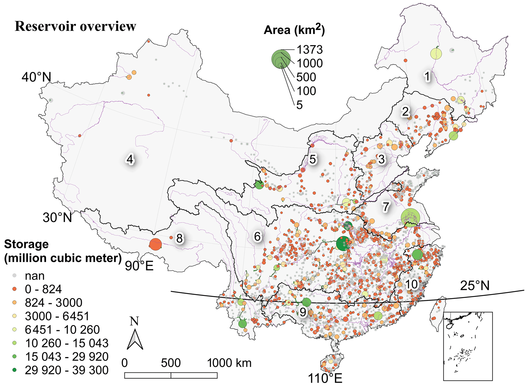
Figure 1Overview of the reservoirs contained in Res-CN and the dams with storage capacity (circle color; nan means not available) and water surface area of reservoirs (circle size). The black lines indicate the boundaries of the 10 river regions within Res-CN. Numbers (1–10): 1 – Songhua River; 2 – Liao River; 3 – Hai River; 4 – Northwest River; 5 – Yellow River; 6 – Yangtze River; 7 – Huai River; 8 – Southwest River; 9 – Pearl River; 10 – Southeast River regions.
In addition to the time series of reservoir datasets described above, reservoir upstream catchment attributes (e.g., climate, geology and soil, topography, land cover, and anthropogenic activity characteristics) are also important as reservoirs collect materials from upstream catchments. These attributes affect the water balance and water quality of a reservoir, such as temperature, dissolved oxygen, and turbidity (Yang et al., 2022). Moreover, the limnological properties of one reservoir have the potential to impact other reservoirs through the transfer of water mass, nutrients, energy, and sediments via connecting rivers, as previously demonstrated in studies by Huziy and Sushama (2017) and Stieglitz et al. (2003). Thus, researchers can better understand catchment-level landscape limnology by incorporating these attributes (Soranno et al., 2010). The values of these catchment-level attributes are also proved in the Catchment Attributes and MEteorology for Large-sample Studies (CAMELS) dataset, introduced by Addor et al. (2017), and follow-up studies such as CAMELS-CL, CAMELS-BR, CAMELS-GB (Alvarez-Garreton et al., 2018; Chagas et al., 2020; Coxon et al., 2020), LamaH-CE (Klingler et al., 2021), CCAM (Hao et al., 2021), LakeATLAS (Lehner et al., 2022), and the studies by Chen et al. (2022) and Liu et al. (2022). However, there is a data gap of reservoir-catchment characteristics in China and even in the geometric boundaries of reservoir upstream catchments, which hindered the spatially explicit applications of such catchment information. Furthermore, allocating reservoirs on river networks is also valuable for river models incorporating reservoirs, as reservoir datasets and river network datasets are usually developed independently and are not corresponding well, which could cause some issues when integrating reservoirs into river models.
In light of the above, we build upon these existing studies and datasets to produce a new publicly available comprehensive and extensive reservoir dataset, Res-CN (Reservoir dataset in China). It is based on the latest global reservoir shapefiles from GeoDAR v1.1. Additionally, we allocate reservoirs in MERIT Hydro (Yamazaki et al., 2019) to delineate reservoir catchments into two categories: full catchments and intermediate catchments. The 512 catchment-level attributes for 3254 reservoirs are generated at full catchments and intermediate catchments from a wide range of satellite-, reanalysis-, and in situ-based data. Besides these, time series of reservoir states (i.e., water level, water surface area, storage anomaly, and evaporation) are extracted from multiple altimeters, Landsat and Sentinel images, and other satellites, acting as a key supplement to existing products owing to their significantly enhanced spatial and temporal coverages. In situ data of 138 reservoirs are employed in this study as a valuable reference for evaluation, thus enhancing the confidence in the data quality and enhancing the understanding of the accuracy of current satellite datasets. Our codes, in Python, R, and GEE (Google Earth Engine), are freely available and open source. The codes can be applied to individual applications or other areas, and they can further enrich the inventory if new data become available. Results of this study facilitate the management of reservoirs and relevant studies such as hydrological modeling, environmental studies, and climate research in the spatially explicit context of reservoir catchment level (Galelli et al., 2022; Dang et al., 2020).
China has more than 98 000 reservoirs and dams across different topographic regions and landscapes (MWR, 2016). However, most of them are unmapped (polygons and georeferenced coordinates are not available) and only described with standard attributes. Thus, in this study, we focused on reservoirs which are mapped and available from the newest global GeoDAR database (Wang et al., 2022). GeoDAR v1.1 provides global reservoir shapefiles and their attributes such as storage capacity, reservoir purpose, and installed capacity. Reservoirs are mostly clustered in the Yangtze and Pearl River basins (Fig. 1) and vary greatly in size, capacity, and purpose.
As we aim to create a comprehensive reservoir dataset in China, our workflow required multiple steps and geospatial techniques. Here, we detail the data and methodologies that are applied to create water level, water surface area, storage anomaly, evaporation, upstream catchment boundaries, and catchment-level characteristics. The flowcharts and source datasets are provided in Figs. A2, A3, and S1–S3, as well as Tables S2–S8 in the Supplement.
2.1 Data and methodology for generating reservoir water level
Water level time series for the Res-CN dataset are derived from various satellite altimeters: Sentinel-3A, Sentinel-3B, Jason-3, ICESat-2, CryoSat-2, and SARAL/AltiKa. Each altimeter has different repeat cycles, geographical coverages, retracking algorithms, and measurement accuracies (Table S2). Apart from the official algorithms in their source products, we implemented PPCOG (primary peak center of gravity) and NPPTr[0.5/0.8] (narrow primary peak with a 0.5 or 0.8 threshold value) algorithms into Sentinel-3, CryoSat-2, and SARAL/AltiKa to derive range measurements (Shen et al., 2022a). Range measurements are corrected using the atmospheric and geophysical corrections from their source products (Table S2), and they are then used to determine the water level of each sample. We reference the height to the EGM2008 geoid (Pavlis et al., 2012).
For the construction of reservoir water levels, we carried out the following steps to process single-satellite altimetric heights from each retracking algorithm (Fig. S1):
-
We extracted the altimetric data within the GeoDAR reservoir shapefile.
-
The Global Surface Water Explorer was used to select altimetric data for which water occurrence is greater than 10 % (Zhang et al., 2020).
-
We removed outliers for each pass using the MAD method (median of absolute deviation).
-
We removed outliers from altimeter data with heights of more than 20 m from the DEM (for reservoirs with large variations, we set a threshold of 40 m).
-
We constructed time series using the R package “tsHydro” (Nielsen et al., 2015).
Through these steps, each satellite altimeter's SR (standard-rate) water level time series with different retracking algorithms was produced. A single-satellite altimeter's repeat period and spatial sampling result in a low resolution for SR products. For example, with Sentinel-3A ground tracks spaced 104 km apart at the Equator, it may be possible to obtain altimetric data on 684 GeoDAR reservoirs in China. For increased resolution and to overcome the limitations of single-satellite altimeter spatial and temporal sampling, we generated HR (high-rate) water level time series products by integrating single-satellite SR products. Note that we used altimetric observations from multi-missions using the retracking algorithm with the smallest RMSE (root-mean-square error) value calculated with in situ water level. To eliminate systematic differences between satellites, we used two methods: the first method is by directly eliminating the mean water level differences between satellites and is applicable to satellites with sufficient overlap periods; the second method is to estimate satellite bias using reservoir water areas. The bias was estimated by minimizing the two-dimensional cost function of area–water-level coordinates using the Gauss–Helmert method (Fig. S1). To evaluate the altimetric data quality, we calculated the standard deviation (SD) of altimetric observations and RMSE values against in situ water level and three other similar existing products from Hydroweb, DAHITI, and G-REALM wherever available. Data point precision is determined by SD, whereas accuracy is determined by RMSE. RMSE is calculated by comparing water level anomalies between gauges and satellites. In situ water level data of 99 reservoirs from 2015 to 2021 are used to validate our dataset.
2.2 Data and methodology for generating reservoir water surface area
Reservoir water surface areas can be extracted from an available global inland water dataset like SWBD (SRTM Water Body Data; NASA JPL, 2013), GIEMS (Global Inundation Extent from Multiple Satellites; Papa et al., 2010), GSW (Global Surface Water), DAHITI, Hydroweb, Hydrosat, Bluedot Observatory, and studies from Tortini et al. (2020) and Shen et al. (2022a). The derived reservoir water surface area estimations are limited by the spatial coverage and accuracy restrictions of the initial dataset. As such, three available global water surface area products are developed by using algorithms that reclassify contaminated pixels as water, i.e., GRSAD (Zhao and Gao, 2018), RealSAT (Khandelwal et al., 2022), and areas of medium-to-small reservoirs by Donchyts et al. (2022). These products cover only a portion of the reservoirs we studied (e.g., 908 overlapping reservoirs between GRSAD and our product) and use different algorithms and source datasets (e.g., RealSAT and GRSAD use only Landsat). As a part of this study, we employed the algorithm developed by Donchyts et al. (2022) to generate reservoir water surface areas by using Landsat and Sentinel-2 images. The algorithm has been applied to map water surface areas in 768 reservoirs of different sizes and climate zones located in Spain, India, South Africa, and the USA, and there is strong evidence to suggest that it performs well in this regard (Donchyts et al., 2022). For a given reservoir, the procedures are as follows.
A selection of cloudy satellite images intersecting the reservoir shapefile is made.
Based on the global cloud frequency dataset (Wilson and Jetz, 2016), we filtered out satellite images that were completely covered by clouds and corrected the remaining images as follows:
-
We calculated the NDWI (normalized difference water index).
-
A Canny edge detection algorithm was used for detecting water/land edges and defining sampling areas around them (Donchyts et al., 2016).
-
We utilized the Otsu algorithm (Markert et al., 2020) to determine the optimal threshold value; we then obtained the water mask based on samples of NDWI values collected within the sampling area.
-
We sampled the water occurrence along the edges to eliminate falsely detected water (water pixels that were not water).
-
Water occurrence was clipped at a certain occurrence value and combined with the water mask to obtain the final water mask.
-
We used a quantization-based temporal outlier filter to remove any errors from reservoir waters.
Using these procedures, we generated monthly reservoir water surface areas during 1984–2021. We evaluated the data quality by comparing it to in situ water levels, altimetry (HR and SR products) whenever available, and previously available products from GRSAD and RealSAT. The indicators of data quality were rBIAS (relative bias), CC (Pearson correlation coefficient), and rRMSE (relative RMSE).
2.3 Data and methodology for generating reservoir storage anomaly
Res-CN estimates of reservoir storage anomaly are based on (1) satellite-based water levels and water surface areas and (2) water surface areas and DEMs (digital elevation models) (Fig. S2 in the Supplement). The basis of these two approaches is a reconstruction of the hypsometry curve (water surface-area–level model) using overlapping records of water level and water surface area or DEM. Assuming five models (linear, polynomial, exponential, power, and logarithmic) can be used to describe hypsometry curves, we selected the model with the highest R2 value as the reservoir's hypsometry curve. We followed the following steps for reservoirs with both water level and water surface area records:
-
We used the average of all altimetric measurements in a month to calculate the monthly reservoir water level.
-
A scatterplot of monthly water level and water surface area was constructed, and errors were eliminated from the scatterplot.
-
A parametric approach was used to generate the hypsometry curve (i.e., the water surface-area–level model).
-
We estimated the gap measurements of water levels and water surface areas by applying the reconstructed hypsometry curve.
-
We calculated storage anomaly ΔV from two successive pairs of water-level–water-surface-area measurements (H, A) (Eq. 1).
For reservoirs with water surface areas only, we used the DEM-based approach. The main procedures are described below:
-
generating the water surface-area–level–storage model through a DEM-based approach (Vu et al., 2022),
-
calculating storage anomaly by combining satellite-based water surface areas and the area–level–storage model.
As a result of these steps, we determined the hypsometry curve and time series of storage anomalies for each reservoir.
To evaluate the storage anomaly data, we calculate the error statistics of RMSE, NRMSE (normalized root-mean-square error), and CC values for reservoirs with in situ observations. In situ water storage data of 138 reservoirs from 2015 to 2021 are used to validate our dataset.
2.4 Data and methodology for generating reservoir evaporation
Reservoir evaporation estimates can be extracted from two available global reservoir evaporation products produced by Zhao et al. (2022) and Tian et al. (2022). These studies covered a portion of the reservoirs we studied and used the same robust algorithm by Zhao and Gao (2019) to calculate monthly reservoir evaporation volume (VE, m3 per month) using water surface area (A, km2), days of a month (days, –), and evaporation rate (Ereservoir, mm d−1) (Eq. 2).
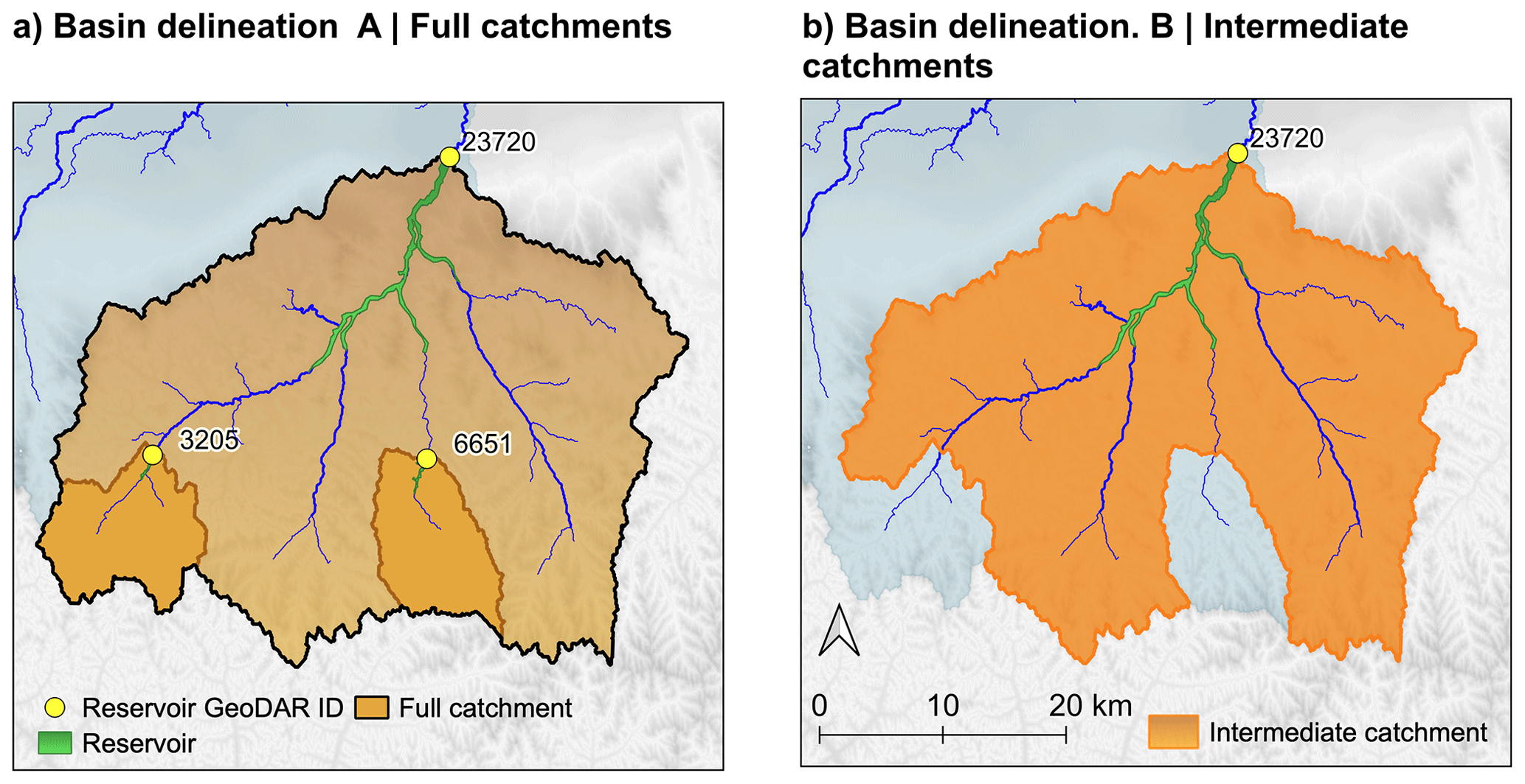
Figure 2An example of the types of catchment delineations in Res-CN. (a) Catchment delineation A: full catchments, which are defined as the entire area contributing to a reservoir. In plot (a), full catchment of reservoir 23720 overlaps with that of reservoir 3205 and that of 6651. (b) Catchment delineation B: intermediate catchment. In plot (b), all upstream contributing areas of the upstream reservoirs (3205 and 6651) are removed from the full catchment of reservoir 23720; thus, we get the intermediate catchment of reservoir 23720 (in black boundary). Background in light blue indicates other catchments not shown in this example. Source of background: MERIT Hydro and MERIT DEM (Yamazaki et al., 2019).
In this study, we applied the algorithm while considering its satisfactory simulation performance for the evaporation rate and energy balance terms (Eqs. 3 and 4). It quantifies heat storage changes (δU, ) in the Penman equation:
where Ereservoir is the reservoir evaporation rate (mm d−1); Δ is the slope of the saturation vapor pressure curve (); Rn is the net radiation (); γ is the psychrometric constant (); λ is the latent heat of vaporization (MJ kg−1); u2 is the wind speed at 2 m height (m s−1); Lf is the monthly reservoir fetch length (m); es and ea are the saturated vapor pressure at air temperature and the air vapor pressure (kPa), respectively; ρw is the density of water (kg m−3); cw is the specific heat of water (); h is the average water depth (m); Tw and Tw0 are the water column temperature at the current time step and at the previous time step (∘C), respectively; and Δt is the time step (set as 1 month in this study).
It is worth noting that this algorithm does not need parameter calibration and only requires Lf, h, and four meteorological variables (air temperature, ∘C; wind speed, m s−1; vapor pressure deficit, kPa; and surface downward shortwave radiation, ) for the evaporation rate calculation. In previous studies (Zhao et al., 2022; Tian et al., 2022), the TerraClimate dataset (Abatzoglou et al., 2018) has been shown to be the most appropriate meteorological dataset for reliable estimates of reservoir evaporation rates compared to other global datasets. Thus, we adopted the TerraClimate to generate meteorological data time series by averaging gridded forcing data within reservoir shapefiles. Monthly reservoir fetch values, Lf, were calculated using (1) reservoir shapefiles, (2) wind direction data from the NCEP (National Centers for Environmental Prediction), and (3) water surface area time series. The average reservoir water depths, h, are taken from the GRanD and HydroLAKES datasets. For reservoirs not recorded in these two datasets, we determined their water depths from their water surface areas through the area–depth curves fitted to all available data. A detailed algorithm flowchart, all equations, and examples are provided in Fig. S3 and in Zhao and Gao (2019).
2.5 Data and methodology for generating reservoir catchment boundaries
In this study, two types of reservoir upstream catchment boundaries (hereafter referred to as catchment) are defined: full catchments and intermediate catchments (Fig. 2). The full catchment is defined as a reservoir's full upstream contributing area, whereas the intermediate catchment is determined by subtracting the area contributed by upstream reservoirs from the catchment area of the current reservoir. Obviously, full catchments are independent of each other, but for reservoirs with larger catchments, they can lead to a significant loss of information such as the local features and variability. Thus, intermediate catchments, which are part of the large river networks, can complement this information, and this ensures more representative and accurate mapping of local variables.
To identify catchment boundaries (Fig. A2), we used an automatic outlet relocation algorithm (Xie et al., 2022) to automatically delineate a large number of catchments. This algorithm can correct the river networks by analyzing the gradients of flow accumulations along the rivers and can rapidly delineate catchments (Xie et al., 2022). More importantly, it has been intensively validated for 1398 catchments of varying size and geographic regions, showing that 94.1 % of catchments were correctly delineated. This algorithm requires the flow directions and gauge locations as input. In this study, we used flow directions from MERIT Hydro and dam locations from the GeoDAR dataset. MERIT Hydro is a new global hydrography map that has a fine resolution of 90 m and shows good performance in terms of river basin shape and flow accumulation area. This algorithm can generate the full catchments of each reservoir, and we employed some additional operations to remove topology errors and obtain intermediate catchments. Firstly, we cleared the holes to remove topology errors across full catchments. Secondly, we checked the full catchments and removed the unrealistic or incorrect catchments. Thirdly, we generated intermediate catchments by removing the overlapping areas of upstream reservoirs from the full catchment of the current reservoir using QGIS 3.24. Lastly, we fixed the invalid geometry of intermediate catchments by eliminating geometry errors (Text S1 in the Supplement).
2.6 Data and methodology for generating catchment-level characteristics
Catchment attributes can be categorized into six types: reservoir and catchment body characteristics, climate, geology and soil, topography, land cover, and anthropogenic activity characteristics. The sources for different datasets were chosen to ensure use of high-quality data, the most reputable sources, global coverage, theoretical impacts on reservoirs, and high spatial resolution as far as possible. For example, the NSCD version 3 (National Station-based Climatic Data set) is the most widely used in situ meteorological dataset in China, while MERIT DEM is a widely used global hydrography map. Here, we give a brief description of data processing, while the detailed interpretations, uncertainties, and limitations of source datasets are available in Sect. 3, the Supplement, and Fig. A3 in the Appendix.
Some necessary data format conversions (e.g., netCDF to raster format) and reprojections are firstly conducted for related attribute datasets. Then, we used different methods to calculate catchment-level characteristics from raster and vector data. Statistics values were calculated for raster grids within each catchment. In the case of continuous variables such as temperature and elevation, we calculated their mean, maximum, minimum, and range values. For categorical variables such as geological maps and land use features, we calculated the percentages of each variable and determined their dominant type. The implementation for processing raster data is done in the local Python and R environments (package: rasterstats) and the GEE platform. For vectorial data such as the rivers and catchments in ESRI shapefile format, the shape features of each catchment are calculated using the local Python scripts, and other catchment attributes like stream density are determined by the ratio of the intersection area between the vectorial data and the catchment extent layer to the total catchment area. After repeating these procedures for each catchment, catchment-level attributes are prepared for both full catchments and intermediate catchments.
3.1 Description of the Res-CN database
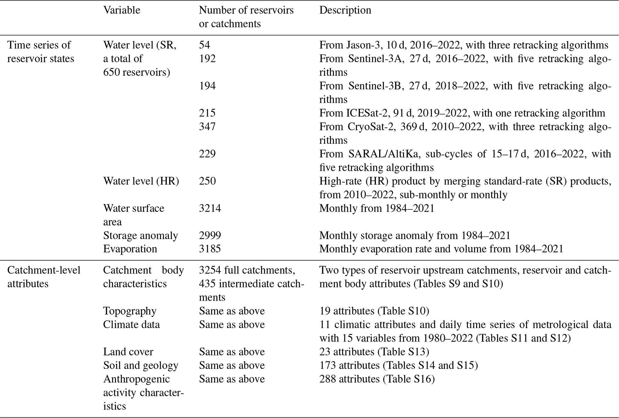
We here provide summarized information on the components of Res-CN in Table 1. Detailed descriptions of each component are shown in the following sections and in the Supplement. In this study, we constructed reservoir-catchment characteristics for 3254 reservoirs recorded in the GeoDAR database (Wang et al., 2022) with water surface areas ranging from 0.004 to 1373.77 km2 (Fig. S4) and storage capacity totaling 682 595 km3 (73.2 % of reservoir water storage capacity in China). Using both full catchments and intermediate catchments, characteristics of reservoir catchments were extracted, with a total of 512 attributes in six categories (Table 1). Besides, time series of reservoir states such as water level and water surface area are also provided, with their comprehensive evaluation reports (i.e., statistics and figures in PDF and Excel files) based on in situ data when available. For more details, please refer to the data repository and the following sections.
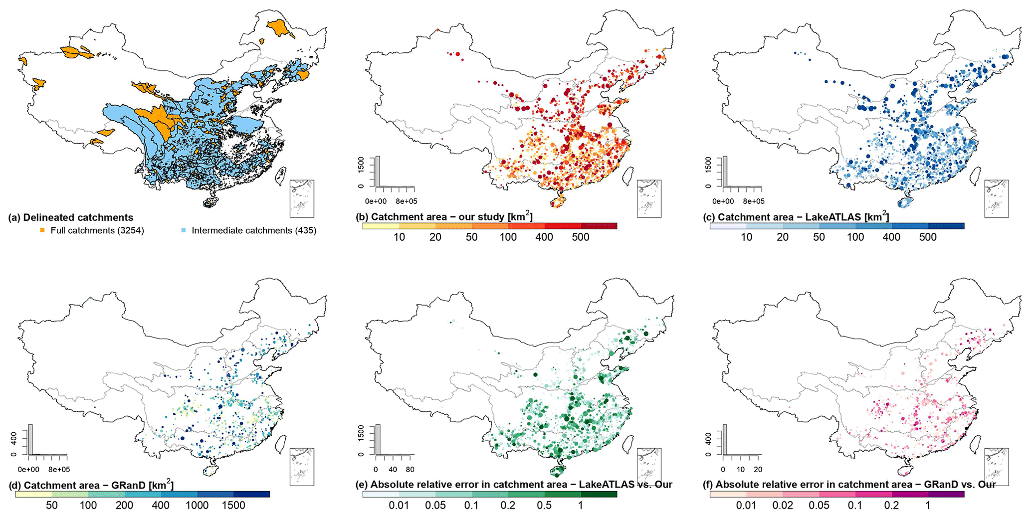
Figure 3Distribution of the delineated catchments (intermediate catchments and full catchments). Each category's histogram indicates the number of basins (out of 3254). In a histogram, the x axis represents the number of basins, while the y axis represents each subplot's caption. Circle sizes are proportional to catchment areas.
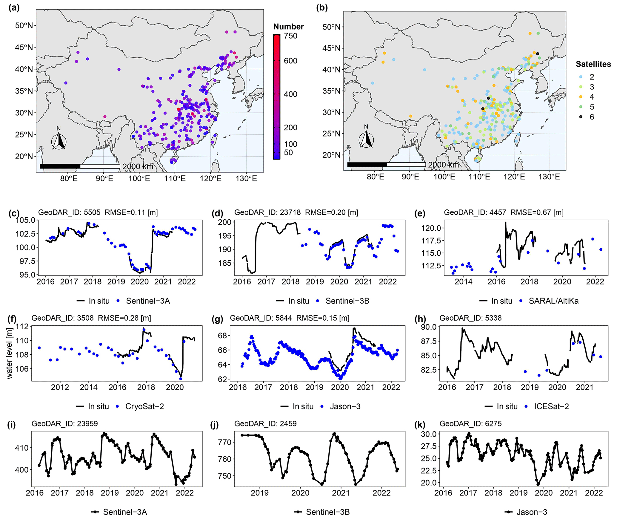
Figure 4Data availability of the altimetric reservoir water level time series (a) and number of satellites for high-rate products (b) as well as some examples to illustrate time series of standard-rate products over nine selected reservoirs (c–k).
3.2 Res-CN products for the delineated catchment characteristics
Res-CN provides 3254 full catchments and 435 intermediate catchments (Fig. 3). The median catchment size of full catchments is 294 km2, with a range of 0.94 to 981 473 km2. The plausibility of full-catchment delineation was assessed by comparing the area of the delineated catchments with the areas of two declared references: GRanD (Lehner et al., 2011) and LakeATLAS (Lehner et al., 2022). LakeATLAS delineated upstream drainage area of more than 1.4 million lakes and reservoirs globally based on the lake pour points and the 15 arcsec drainage direction grids of HydroSHEDS. A similar approach was applied in GRanD to estimate the areas of upstream catchments over 7320 reservoirs globally. To compare Res-CN with GRanD and LakeATLAS, we spatially joined reservoir shapefiles from both datasets, matching reservoirs that overlapped for greater than 90 % of their extent. Based on this subset of reservoirs, we found that catchment areas delineated in this study corresponded relatively well to catchment areas in both GRanD (CC = 0.99, n = 910) and LakeATLAS (CC = 0.91, n = 2147), which proves the reliability of our delineated catchments. Large discrepancies occur in 55 catchments, whose absolute relative error is greater than 100 % (Fig. 3e and f). Small reservoirs located near confluences between rivers of different sizes are more likely to be affected by this issue, as a minor spatial mismatch can assign a reservoir to the small catchment of the tributary stream rather than the large catchment of the mainstream, and vice versa (Fig. S5). The differences in catchment delineation between these datasets result from differences in both DEM and methods for flow direction correction and depression filling and pour point correction. In this study, the widely verified MERIT Hydro flow directions at 3 arcsec are used, and we suggest that caution should be taken when using catchments with large error discrepancies with LakeATLAS, which is based on the 15 arcsec drainage direction grids of HydroSHEDS (Fig. S5a). Intermediate catchments provide information regarding the variability of local features and the upstream–downstream relationship. The median catchment size of intermediate catchments is 936 km2, with a range of 1 to 279 424 km2.
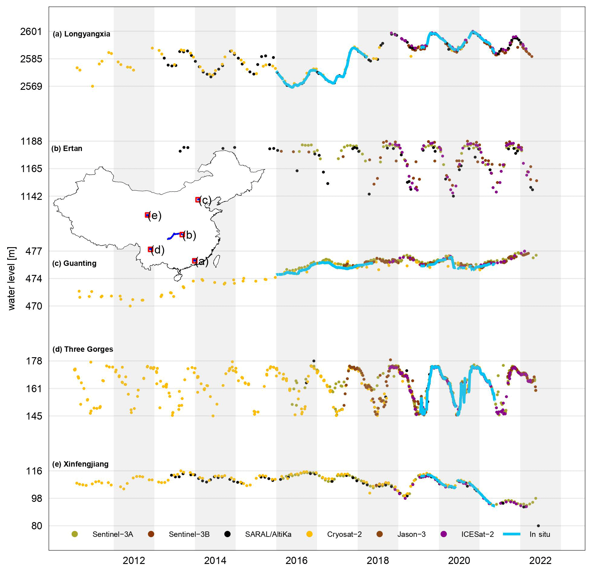
Figure 5High-rate water level time series over reservoirs Xinfengjiang (264 km2) from Sentinel-3A, SARAL/AltiKa, Sentinel-3B, CryoSat-2 and ICESat-2; Three Gorges (852 km2) from Sentinel-3A, SARAL/AltiKa, Sentinel-3B, CryoSat-2, ICESat-2, and Jason-3; Guanting (90 km2) from Jason-3, CryoSat-2, ICESat-2, Sentinel-3A, and Sentinel-3B; Ertan (65 km2) from Jason-3, SARAL/AltiKa, ICESat-2, Sentinel-3A, and Sentinel-3B; and Longyangxia (285 km2) from SARAL/AltiKa, CryoSat-2, ICESat-2, and Sentinel-3B.
3.3 Res-CN products for time series of reservoir states
3.3.1 Reservoir water level
There are two modes of reservoir water level time series available from Res-CN: SR and HR. Figure 4 demonstrates their spatial coverages, data source and availability, and evaluation reports against in situ observations. Among them, over 200 reservoirs are visited by CryoSat-2, SARAL/AltiKa, and ICESat-2, and only 192 and 54 reservoirs are covered by Sentinel-3A and Jason-3, respectively (Table 1). Data quality was generally good for smaller RMSE values (< 0.3 m), moderate for those between 0.3 and 1.0 m, and relatively poor for those greater than 1.0 m. For each altimeter and HR product, the percentages of validated reservoirs with good, moderate, and poor data quality are 44 %, 33 %, and 23 % (Sentinel-3A: validated in 34 reservoirs); 55 %, 18 %, and 27 % (Sentinel-3B: 22); 38 %, 37 %, and 25 % (SARAL/AltiKa: 8); 71 %, 10 %, and 19 % (ICESat-2: 31); 50 %, 36 %, and 14 % (Jason-3: 14); 22 %, 56 %, and 22 % (CryoSat-2: 27); and 25 %, 73 %, and 2 % (HR products: 84). We found that in most cases there is no notable difference in terms of RMSE values between different retracking algorithms (Fig. S6). It should be noted that multisource altimetric measurements are merged for a specific reservoir by using the SR time series with the lowest RMSE from the retracking algorithm. Figure 5 shows examples of the HR products over a sample of six reservoirs with different areas. Single-satellite altimetric time series capture reservoir water level dynamics well, leading to improved temporal resolution of the HR product. A cross-validation of the time series against other existing databases as well as a comparison of their spatial coverage in China (Table S1 and Fig. S7) further demonstrated the advantages of our products. Water levels provided by Res-CN generally agree with those provided by existing similar products (Hydroweb, G-REALM, and DAHITI) with CC values exceeding 0.9, although there are some discrepancies. As an example, Res-CN time series are much denser and less noisy than Hydroweb's in most reservoirs. At the Sanhezha reservoir, G-REALM failed to capture the clear fluctuation pattern, while large discrepancies were apparent at the Fengman reservoir in 2020 between Res-CN and Hydroweb (Fig. S7).
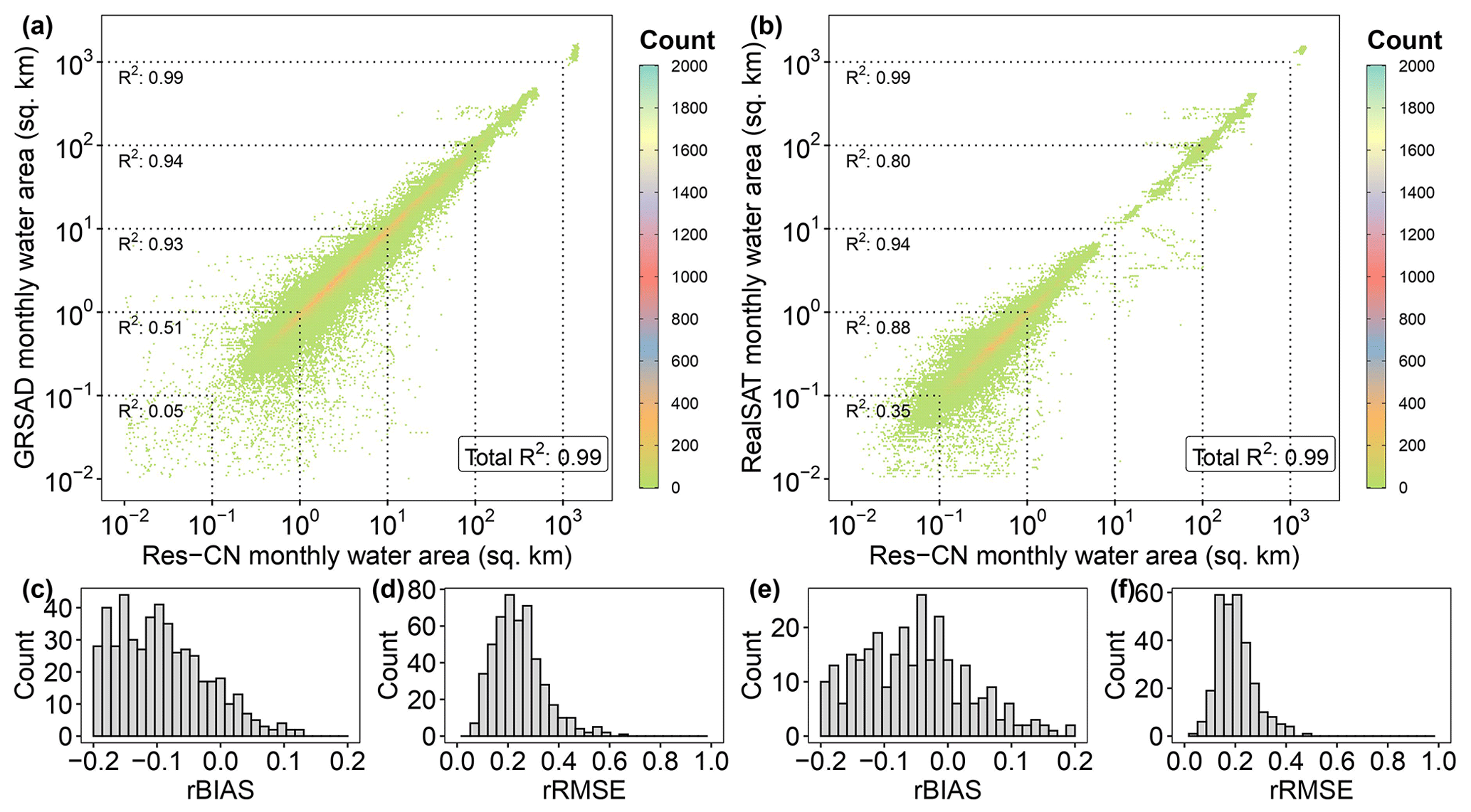
Figure 6Cross-validation of reconstructed monthly reservoir area values by comparing to two existing global datasets. (a, c, and d) Comparison between reconstructed monthly reservoir areas and GRSAD. (b, e, and f) Comparison between reconstructed monthly reservoir areas and RealSAT.
We should consider some limitations for further improvements despite our products' good performance and expanded spatial coverage. We provided the uncertainty information for each value of the time series in the data product file. The SD (standard deviation) estimates can quantify the accuracy of the water level along the track at the level of individual data points (Fig. S8). Water level time series for each reservoir are available in Rec-CN as Excel files, PDF files, and detailed evaluation reports based on in situ data when available (see “Data availability” section and Fig. S9). In our study, more than 80 % of reservoirs with inadequate altimetric measurements are removed due to the inherent limitations of satellite altimeters. There are still challenges to delivering useful measurements for certain reservoirs along the Yangtze and Yellow rivers, and data quality is poor in terms of RMSE values regardless of reservoir size. It may be possible to apply advanced algorithms, such as machine learning, in future studies to achieve better performance regardless of whether reservoirs represent different behaviors.
3.3.2 Reservoir water surface area
Res-CN provides monthly reservoir water surface area data derived from Landsat and Sentinel-2 images during 1984–2021, along with their detailed evaluation reports (see “Data availability” section). We compare these datasets with in situ water levels and altimetric measurements as well as other areal datasets (GRSAD and RealSAT). RealSAT generated 681 137 monthly lake surface area maps from Landsat images during 1984–2015 using an ORBIT (ordering-based information transfer) approach that has been validated on 94 large reservoirs. As opposed to RealSAT, which generated new static lake polygons from water occurrence data, GRSAD used existing static surface water polygons, HydroLAKES and GRanD, to create monthly areas for 6817 global reservoirs based on Landsat images over the last 35 years. The 139 reservoirs with daily in situ observations generally show good agreement in terms of reservoir area and in situ water level time series with 81 % having CC values higher than 0.5. The CC value is expected to decrease for reservoirs with small areal sizes or steep banks. As an example, the CC values of Gutian and Hengjiang reservoirs (10 and 2 km2) are 0.37 and 0.06, respectively. There is also a high median CC value of 0.70 in Res-CN water surface area against altimetric water level time series. As compared to HR altimetric water levels, approximately 63 % of the 244 compared reservoirs have good CC values exceeding 0.5, including 69 with CC reservoirs values > 0.8. For SR altimetric water levels, approximately 63 % of the compared 557 reservoirs have good CC values exceeding 0.5, among which 212 reservoirs show very good agreement with CC values > 0.8. To compare Res-CN with these two datasets, we spatially joined reservoir polygons from all datasets, identifying reservoirs with more than 90 % overlap. The subset of reservoirs shows good agreement with GRSAD (Fig. 6a, median CC value of 0.65, rBIAS = −10 %, rRMSE = 22 %, n = 488) and RealSAT (Fig. 6b, median CC value = 0.64, rBIAS = −5 %, rRMSE = 20 %, n = 288). Since RealSAT and our collected in situ observations do not overlap, we validated only the GRSAD datasets against in situ water levels. GRSAD also showed a good agreement with CC values higher than 0.5 for 58 % of the 139 reservoirs, including 38 reservoirs that showed a very good agreement with CC values > 0.8. In sum, these comparisons suggest that our dataset is reliable.
Uncertainties in surface water area estimates are generally attributed to satellite images and algorithms. As reported by Zhao et al. (2022), the uncertainty of the Landsat-based GRSAD areal dataset is 6.1 %. In this study, we generated a more reliable reservoir water area product by fusing both Landsat and Sentinel-2 images (Fig. S10), using an algorithm that can largely reduce the impacts of cloud contamination (Donchyts et al., 2022). There is strong evidence to suggest that this algorithm performs well in this regard, as it has been widely validated in 768 reservoirs of different sizes and climate zones located in Spain, India, South Africa, and the USA (Donchyts et al., 2022). Nevertheless, some limitations and future developments should be considered. Our first option is to use Sentinel-1 data to provide more information in cloudy regions. Furthermore, the algorithm may be improved by either the multiclass Otsu algorithm or using advanced machine learning methods.
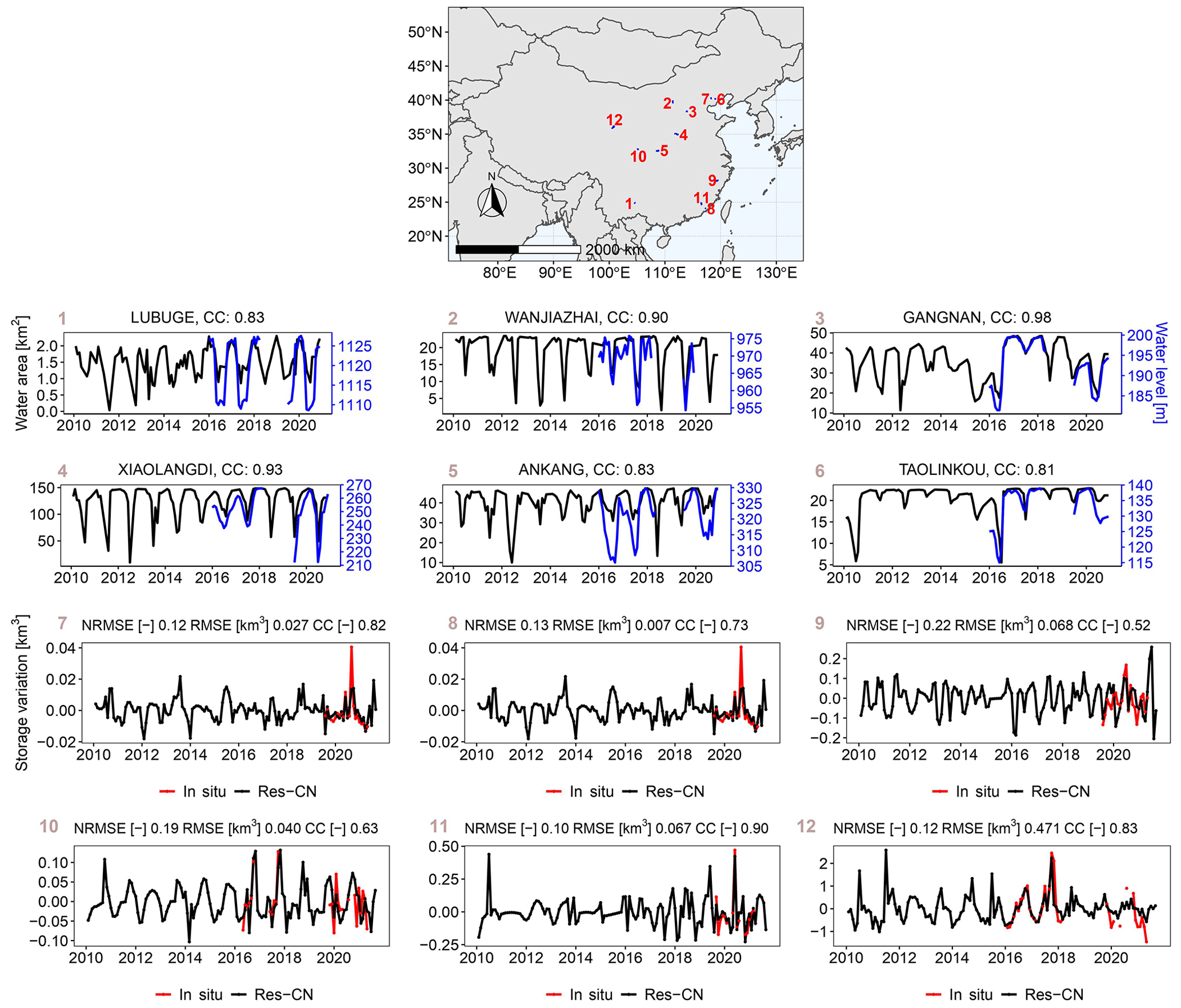
Figure 7Time series of water surface area and storage anomaly in selected reservoirs. RMSE (km3), NRMSE, and CC values are given at the top of each subplot when in situ observations are available. Note that time series of water surface area and storage anomaly of the remaining reservoirs are available in our datasets.
3.3.3 Reservoir storage anomaly
The Res-CN database provides monthly reservoir water storage anomaly for 3254 Chinese reservoirs during 1984–2021 using the DEM's area–storage model, along with their detailed evaluation reports (see “Data availability” section). Seventy-four percent of reservoirs (89 of 119 validated reservoirs with in situ data) have good data quality with a RMSE value below 0.2 km3 and a NRMSE value below 30 %. NRMSE, CC, and RMSE have median values of 21 %, 0.53, and 0.03 km3, respectively. The lowest NRMSE is 7 % in the Luhun reservoir, which has a high CC value of 0.90 and low RMSE value of 0.016 km3. Figure 7 shows variations in water storage in small, medium, and large reservoirs located in different climate zones. The remotely sensed storage anomalies generally agree with the observations represented by the statistical metrics, although some large discrepancies occur in peak values. We find that our error statistics in terms of NRMSE are a bit higher than previous studies in terms of NRMSE below 20 % (Zhong et al., 2020). The errors result from the inaccuracy of the area–storage model developed by the DEM as well as the error of water surface areas at certain reservoirs. To solve this problem, we provide another type of storage variation estimate for 335 reservoirs using satellite water surface areas and water levels (see Sect. 2.3; Shen et al., 2022a). The accuracy of storage anomalies is improved, with median statistics of CC, NRMSE, and RMSE of 0.89, 11 %, and 0.021 km3, respectively.
The uncertainties in storage anomalies are primarily attributed to three sources, i.e., the altimetric water level, water surface area estimations from Landsat and Sentinel-2 images, and the error resulting from their combination (the hypsometric curve). Figure S11 provides an example that illustrates how the uncertainties in satellite datasets propagate to storage anomalies. According to Shen et al. (2022b), the primary source of error in storage anomaly is water surface area and the hypsometric curve. Regarding the water surface area, after applying the algorithm developed by Donchyts et al. (2022), these errors and impacts can be reduced to a large extent. Meanwhile, we employed five hypsometric relationships, and we used the one with the highest R2 value for further use. For more than 80 % of reservoirs, the R2 values are greater than 0.5, providing a strong foundation for storage anomaly estimates. Nonetheless, the current satellite sensors have limitations, as evidenced by the significant discrepancies observed in peak values (Fig. 7). The increasing temporal resolution and data accuracy of satellite datasets, such as the SWOT (Surface Water and Ocean Topography) mission, will likely improve the accuracy of storage anomaly estimates in the future.
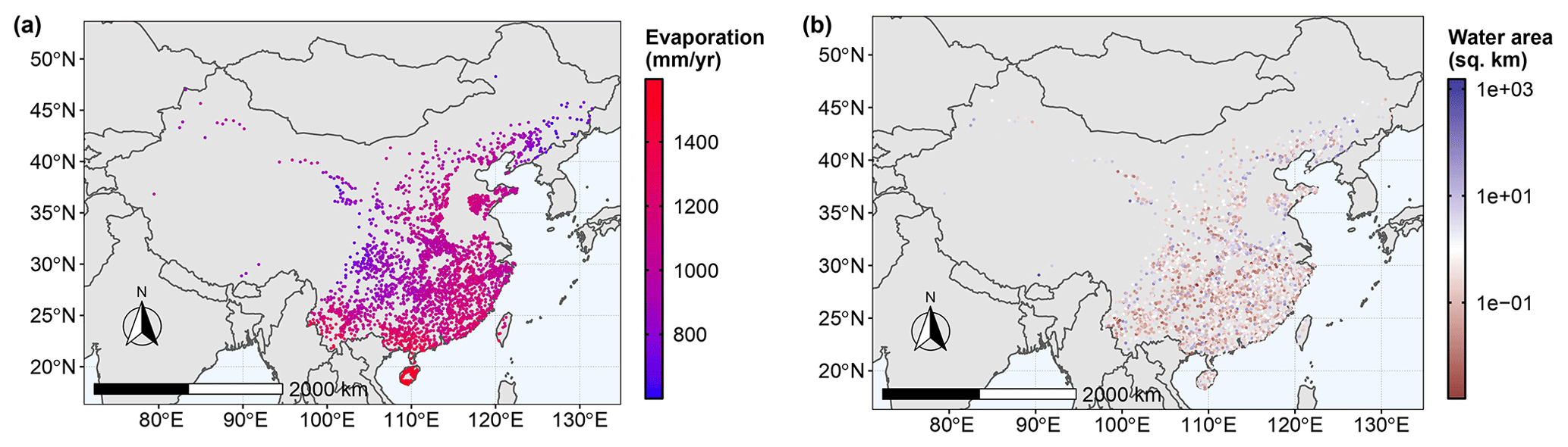
Figure 8Validation of reconstructed monthly reservoir evaporation values. (a) Long-term mean evaporation rates and (b) water surface areas during 1984–2021.
3.3.4 Reservoir evaporation
Res-CN provides monthly reservoir evaporation values for 3254 Chinese reservoirs during 1984–2021. Detailed validations of the algorithm can be found in Zhao and Gao (2019, Zhao et al., 2022) and Tian et al. (2021). The validation of simulated evaporation at an annual scale from Tian et al. (2022) at 47 reservoirs was summarized in Fig. S12 through a literature review. The results in Fig. S12 indicate that the modeled average annual evaporation rates match well with the observed rates. Specifically, the percent bias (PBIAS), Nash–Sutcliffe efficiency (NSE), and root-mean-square error (RMSE) were found to be 0.02 %, 0.82, and 11.2 mm, respectively. This high level of agreement suggests that the Penman method is a reliable approach for calculating reservoir evaporation rates in China. Figure S13 shows the long-term mean meteorological variables that were used to calculate the evaporation rates. We found that reservoirs located in the southern and coastal areas have significantly larger values than other areas due to larger radiation values. For example, the mean evaporation for 613 reservoirs in the Pearl River basin is 1210 mm yr−1, while the mean evaporation for 26 reservoirs in the Songhua River basin is 717 mm yr−1 (Fig. 8a). With respect to the mean reservoir areas (Fig. 8b), small and medium reservoirs are widely distributed across the nation. The CC values between the mean evaporation rates and the surface shortwave radiation, vapor pressure deficit, mean air temperature, and wind speed are 0.88, 0.84, 0.86, and 0.88, respectively.
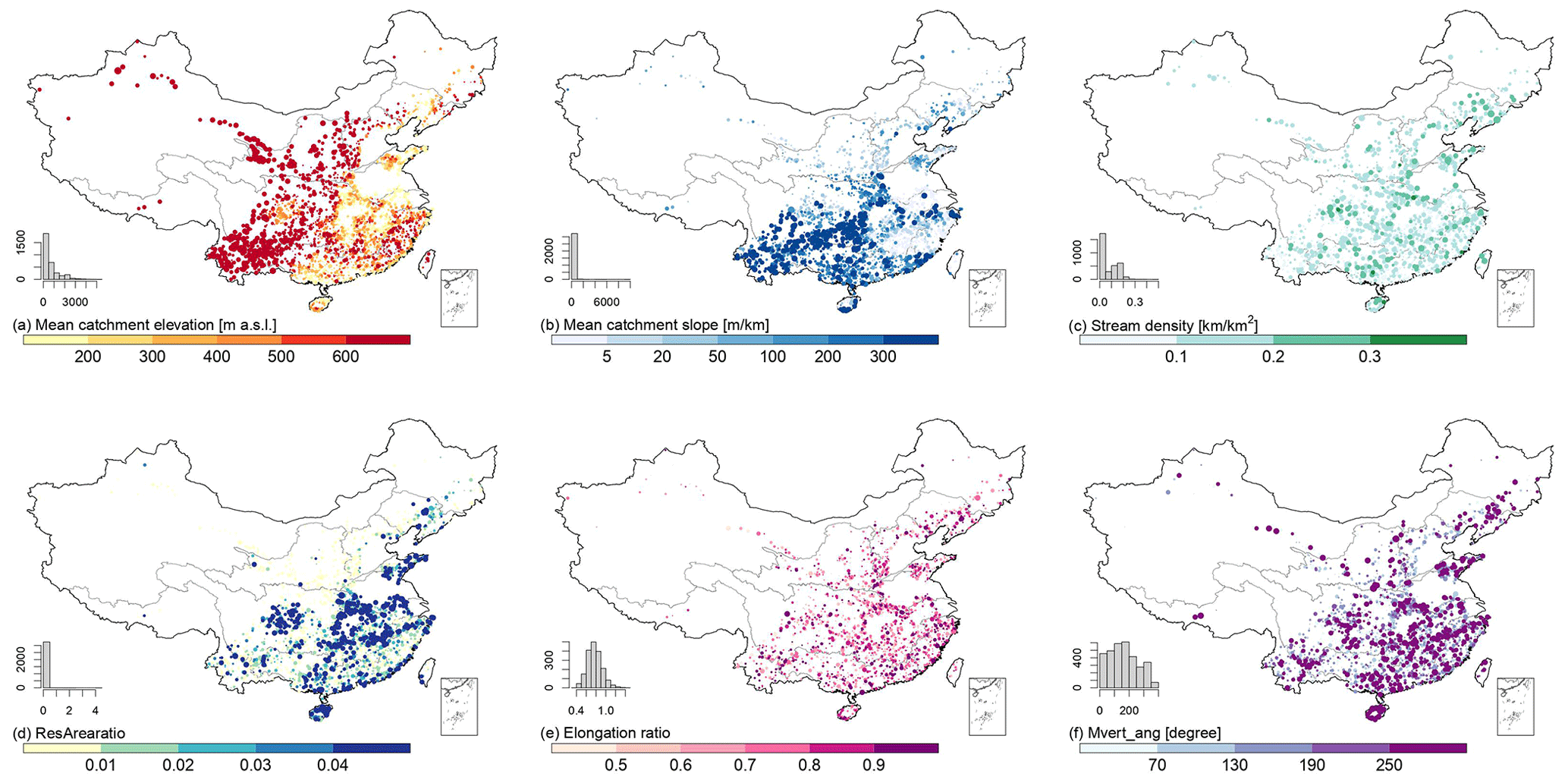
Figure 9Distribution of selected topographic characteristics of intermediate catchments and full catchments. Each category's histogram indicates the number of basins (out of 3254). In a histogram, the x axis represents the number of basins, while the y axis represents each subplot's caption. Circle sizes are proportional to catchment areas.
Despite the good performance of the algorithm, some limitations are worth noting. Uncertainties in the evaporation estimates are generally attributed to three major sources, i.e., the input meteorological forcings, area estimations from Landsat images, and the limitations of the algorithms. As reported by Zhao et al. (2022), the uncertainty of reanalysis datasets is 7.22 %, and the TerraClimate datasets used in this study produce the most reliable evaporation estimates, resulting in a total uncertainty value of 9.93 %. Regarding reservoir water surface area, after applying the algorithm developed by Donchyts et al. (2022), these impacts can be reduced to a large extent. There is some room for improving evaporation rate calculation, such as considering the effects of stratification on water temperature or including the advective heat fluxes from reservoir inflow, outflow, and groundwater.
3.4 Res-CN products for reservoir-catchment-level characteristics
3.4.1 Topographic characteristics
Nineteen topographic attributes are provided in Res-CN (Table S10). The catchment area, slope, and catchment-level elevation (including mean, maximum, minimum, and standard deviation values) were calculated based on MERIT Hydro and MERIT DEM (Yamazaki et al., 2017, 2019). Slope was calculated using the algorithm developed by Horn (1981). Moreover, we determine 10 indices of catchment shapes and stream network as they are vital in runoff generation and flood situations. “mvert_ang” is defined as the angle between the longitudinal axis and the north direction, while “mvert_dist” is a catchment's longitudinal axis distance. These two indices could determine the relative precipitation trajectory in combination with wind speed. “elongation_ratio” is a measure of roundness (i.e., the higher, the rounder) of the catchment and was calculated according to Subramanya (2013). “strm_dens” is often used for comparing catchments as it is a function of many catchment attributes such as climate, soil, and geology. We used the MERIT Hydro database (Yamazaki et al., 2019) to calculate stream density and length within a catchment. The form factor, shape factor, circulatory ratio, and relief of each catchment are also provided. Besides these, we also added “resArearatio” to describe the proportion of the reservoir water surface area and storage to the catchment area (Fig. S14). High average catchment elevations and slopes are most apparent in western China, which extend from the western Yunnan–Guizhou Plateau and southern Qinghai–Tibet Plateau to the northwestern areas (Fig. 9a and b). The streamflow density and resArearatio are relatively high in the central part of the Yangtze River basin, where the artificial reservoirs are densely distributed (Fig. 9c and d). High elongation ratios are widespread in China, and mvert_ang shows high values in the south (Fig. 9e and f).
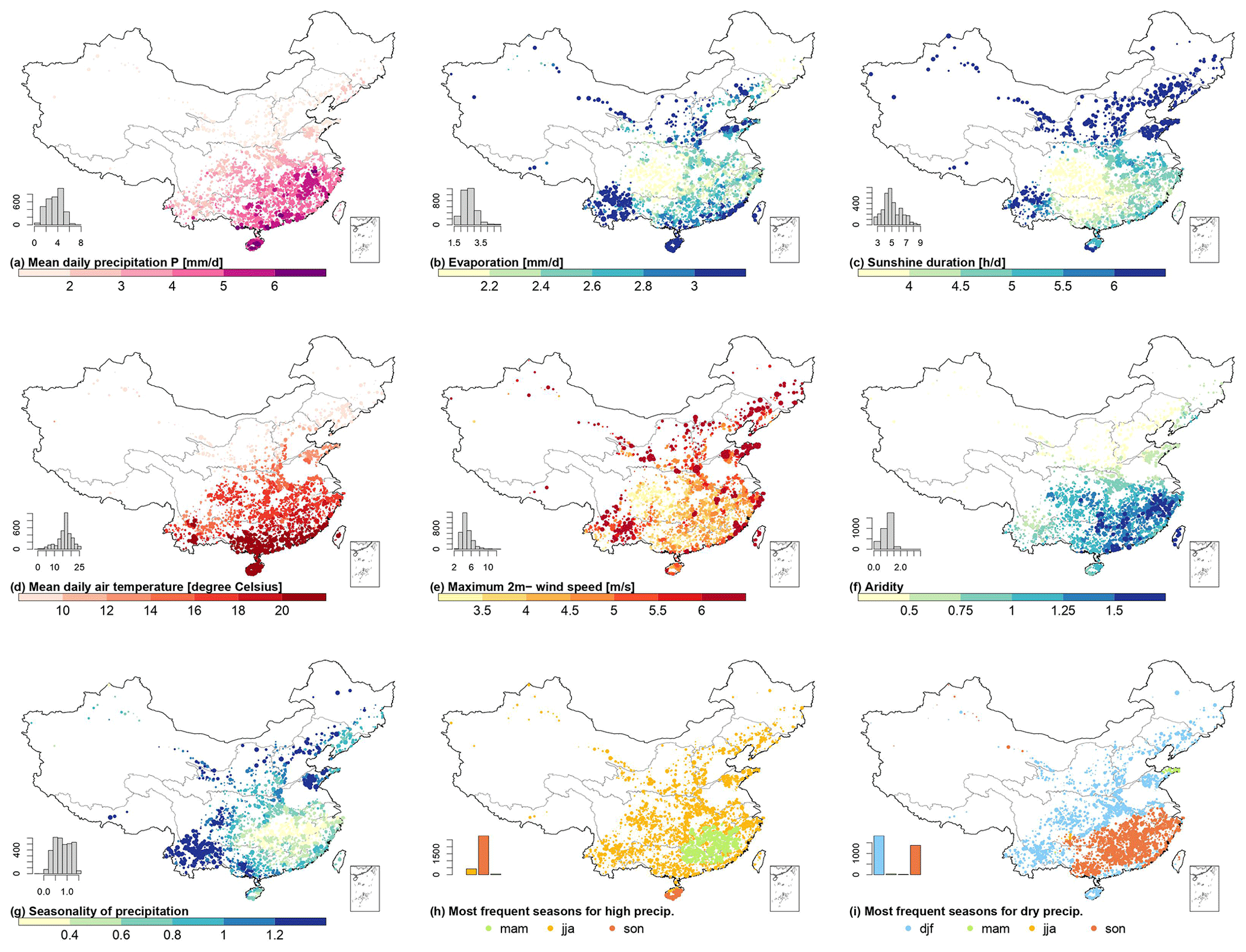
Figure 10Distribution of selected long-term mean meteorological variables and climate indices of intermediate catchments and full catchments. Each category's histogram indicates the number of basins (out of 3254). In a histogram, the x axis represents the number of basins, while the y axis represents each subplot's caption. Circle sizes are proportional to catchment areas.
3.4.2 Climatic characteristics
Res-CN includes daily meteorological time series and 11 attributes reflecting aspects of climatic characteristics (Tables S11 and S12). In this study, we used the National Station-based Climatic Data set V3 (NSCD) to compute the catchment-level climatic characteristics at full catchments and intermediate catchments. NSCD provides daily meteorological time series during 1951–2020 and has near 800 stations in China, with the longest period of gauged observations of precipitation, temperature, evaporation, wind speed, pressure, sunshine duration, relative humidity, and near-surface temperature. The ground sites were sparse before 1970 (Hao et al., 2021). To ensure data quality and to match the periods of other datasets in Res-CN, we used the latter 41 years (from 1980 to 2020) to generate a gridded dataset based on the inverse-distance-weighting interpolation technique (Fig. A2). Figure 10 shows the spatial distribution of selected long-term mean meteorological forcings of full catchments and intermediate catchments. The precipitation and mean air temperature have an increasing trend from northwest to southeast. The sunshine durations are high in the northern areas where latitude is high, and the maximum value is 8.7 h d−1. Wind speed is generally high in the northern mountainous areas, southwestern areas, and coastal parts. The average evaporation is positively correlated with sunshine duration and is higher in the Yellow River basin and southwestern parts.
We calculated nine attributes for NSCD based on meteorological data between 1 October 1990 and 30 September 2020 to reflect aspects of climatic characteristics. Using the Global Aridity Index and Potential Evapotranspiration Climate Database version 3 (Zomer et al., 2022), we derived the reference evapotranspiration (ET0) and aridity index. Aridity is often calculated as a function of precipitation, temperature, and ET0, and it quantifies the precipitation availability for atmospheric water demand. Long-term daily precipitation, reference evapotranspiration, and aridity index (Fig. 10f) characterize the long-term climatic characteristics. The seasonality of precipitation (Fig. 10g) and the fraction of precipitation falling as snow (not shown) are two attributes characterizing seasonality, which yield the yearly maps of sinusoidal precipitation cycle. Short-term events (e.g., heavy rainfall and drought) are characterized by the frequency and duration of heavy precipitation or dry days, as well as their most likely seasons of occurrence (Fig. 10h and i). High precipitation is most likely to occur in summer (Fig. 10h) for 86 % of all 3254 catchments, whereas dry days usually occur in winter (Fig. 10i) for 56 % of them.
One key limitation of the NSCD is that these gauged stations are unevenly distributed across the nation and densely grouped in the eastern and middle parts, which may affect the accuracy for some catchments. Nevertheless, the NSCD meteorological dataset has been widely used as the most reliable observational reference by many studies (Gu et al., 2022). It is produced from a larger number of gauged stations and followed by strict quality-assurance procedures and consistence check. Its accuracy and completeness of each meteorological variable from 1951 to 2020 are significantly improved compared with similar data products in China; the missing rate of data of each element is generally below 1 %, and the correct rate of data is close to 100 %. Relative humidity has a suspicious rate of 0.6 %, large evaporation has a suspicious rate of 1.2 %, and great wind has a suspicious rate of 1.6 %; the suspicious rate of other elements does not exceed 1 / 1000 (Hao et al., 2021). The error rate of sunshine hours is 1 / 10 000, and there are no wrong data for other meteorological variables.
3.4.3 Land cover characteristics
We provide three vegetation indices (EVI, enhanced vegetation index; LAI, leaf area index; and NDVI, normalized difference vegetation index), two indicators of land use (GPP, gross primary productivity; NPP, net primary production), two average rooting depths (50 % and 99 %), and 10 land cover classes in each catchment (Table S13). LAI was derived from the MODIS MCD15A3H dataset with a temporal resolution of 4 d and a spatial resolution of 500 m (Myneni et al., 2015) and used for characterizing vegetation growth. NDVI and EVI were derived from MODIS MOD13Q1 (Didan, 2021) and used to monitor and classify vegetation. These vegetation indices were computed as the maximum, minimum, or difference (e.g., LAImax, LAImin, and LAIdiff). LAImax measures the maximum evaporative and vegetation interception capacity, and LAIdiff shows its temporal variations. GPP and NPP were derived from MODIS MOD17A2H (Running et al., 2021) and MOD17A3HGF (Running and Zhao, 2021) datasets, respectively, and calculated for the whole period of 1 February 2000 to 1 January 2022. Meanwhile, the time series of both vegetation indices and indicators of land use are also provided in Res-CN. Rooting depths are important parameters to characterize the water holding capacity underground and annual evapotranspiration of topsoil. We calculated two average rooting depths (i.e., 50 % and 99 %) based on the IGBP (International Geosphere–Biosphere Programme) classification (Zeng, 2001).
Each catchment was described using 10 land cover classes based on ESA WorldCover 10 m (Zanaga et al., 2021). This dataset is a new baseline of a global land cover product at 10 m spatial resolution for 2020 in almost near real time based on both Sentinel-1 and Sentinel-2 data. Sentinel-1 can provide complementary information on the observed structural characteristics of land cover in areas where the Sentinel-2 images were covered by clouds. Thus, the combination of Sentinel-1 and Sentinel-2 data enables mapping of land cover almost in real time. It includes 11 land cover classes and an overall accuracy of 75 %, providing valuable information for food security, carbon assessment, biodiversity, and climate modeling. The dominant class and fractions of each class were computed with the GEE platform.
Some limitations of these datasets are identified. First, misclassification of ESA WorldCover occurs in areas of irrigated agriculture and wetlands due to the high similarity of their hyperspectral spectrum. Second, although Res-CN provide time series of vegetation indices, it should be noted that NDVI often provides inaccurate measurements of vegetation density, the accuracy of which can only be guaranteed by long-term measurements. In addition, NDVI cannot provide quantitative estimates of vegetation density, so other attributes (i.e., LAI) are provided as a complement.
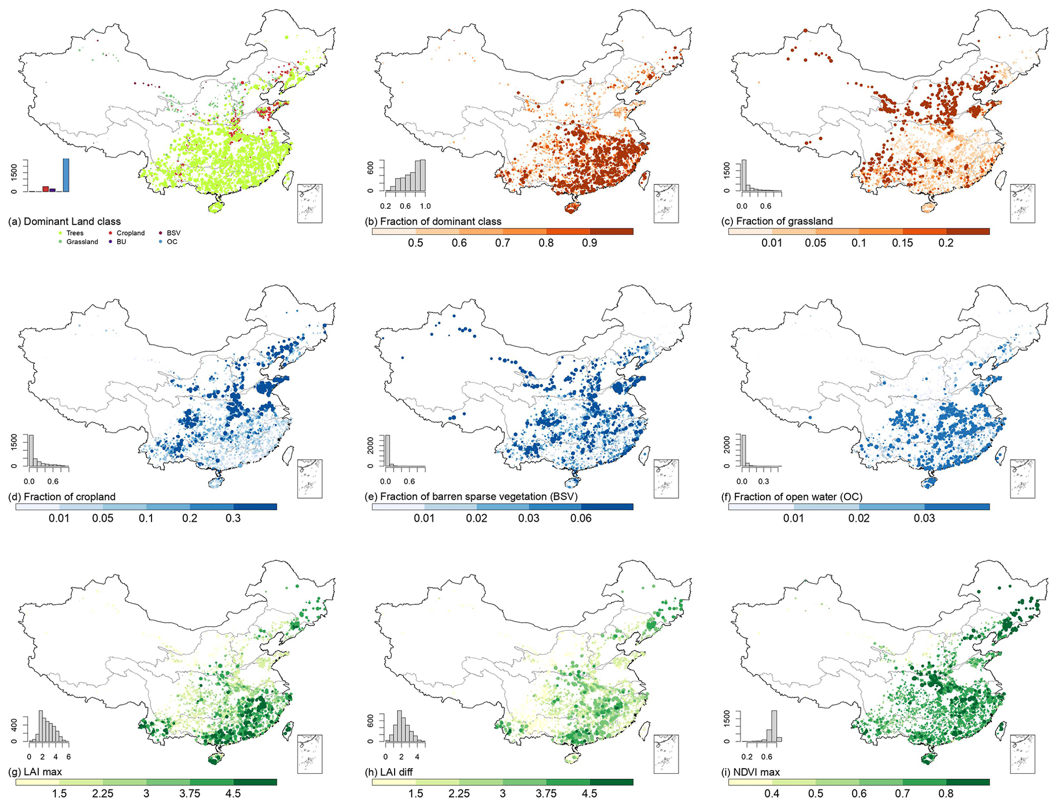
Figure 11Distribution of selected land cover characteristics of intermediate catchments and full catchments. Each category's histogram indicates the number of basins (out of 3254). In a histogram, the x axis represents the number of basins, while the y axis represents each subplot's caption. Circle sizes are proportional to catchment areas.
Trees are prevalent across the nation, and grasslands and croplands are two other dominant land cover types in China. Grassland has higher coverage largely in the Hai River basin and the Yellow River basin (Fig. 11c). Croplands are widespread in China, especially in the Yellow River, Yangtze River, and Huai River basins with a low mean slope (Fig. 11d). Fraction of barren sparse vegetation is quite small across the nation (Fig. 11e). Natural wetlands or waterbodies are mainly distributed in the Yangtze River basin and areas surrounding the Bohai Sea, and these waterbodies are mainly artificial reservoirs and natural lakes (Fig. 11f). Catchments with a relatively high fraction of snow and ice are mainly located in the Tibet Plateau, which is the source region of large rivers in China (not shown). A small proportion of the catchment area is typically considered “built-up”, and 6 % of the catchments have impervious area greater than 0.05 (not shown). There is a spatial correlation between LAImax and LAIdiff with tree fraction (CC = 0.74 and CC = 0.60, respectively). LAIdiff has values similar to LAImax over most areas but should be smaller in areas with a high proportion of trees due to permanent green cover. A negative correlation is evident between the NDVImax (Fig. 11i, CC = −0.78) and the mean catchment elevation (Fig. 9c).
3.4.4 Soil and geology characteristics
Res-CN provided 154 attributes to characterize physical and chemical properties of soil (Table S14). The pH in H2O, cation exchange capacity (CEC), bulk density, and organic carbon content were determined from the SoilGrids250m dataset (SG250; Hengl et al., 2017). The SoilGrids250m dataset predicted soil properties at six different soil layers (i.e., 0–0.05, 0.05–0.15, 0.15–0.3, 0.3–0.6, 0.6–1, and 1–2 m) using machine learning techniques, utilizing data from approximately 150 000 soil profiles and 158 environmental covariates derived from remote sensing data on a global scale. Data within Res-CN are provided for each soil layer and all soil layers using the depth-weighted averaging method. Soil pH is an important variable as it controls many other soil biological, chemical, and physical properties. CEC defines the sum of exchangeable cations that soil can hold and is therefore a measure of fertility and nutrient retention capacity. The density and organic carbon content refer to the mass of organic carbon per unit volume and mass, respectively. Besides SG250, the dataset of soil hydraulic and thermal parameters produced by Dai et al. (2019) was also used. Dai et al. (2019) generated six soil layers of global soil hydraulic and thermal parameters with four products of vertical profiles available using multiple PTFs (pedotransfer functions) based on SG250 and a soil dataset from Shangguan et al. (2014). We adopted the products with the vertical resolutions of SG250 and computed soil characteristics (saturated water content, saturated hydraulic conductivity, and other thermal parameters) for all soil layers. Additional attributes derived from Shangguan et al. (2013) include clay, silt, sand, and rock fragment proportions; soil profile depth; and soil organic carbon (SOC) content. With the use of the polygon linkage method, this database provides soil physical and chemical attributes for land surface modeling in China at a 30 arcsec resolution. Proportions of clay, silt, and sand refer to the fractions of particles < 0.002 mm, particles ≥ 0.002 mm and ≤ 0.05 mm, and particles > 0.05 mm and < 2 mm in the fraction of particles smaller than 2 mm, respectively. SOC is a key variable for ecosystems and affects moisture regimes and ground thermal properties.
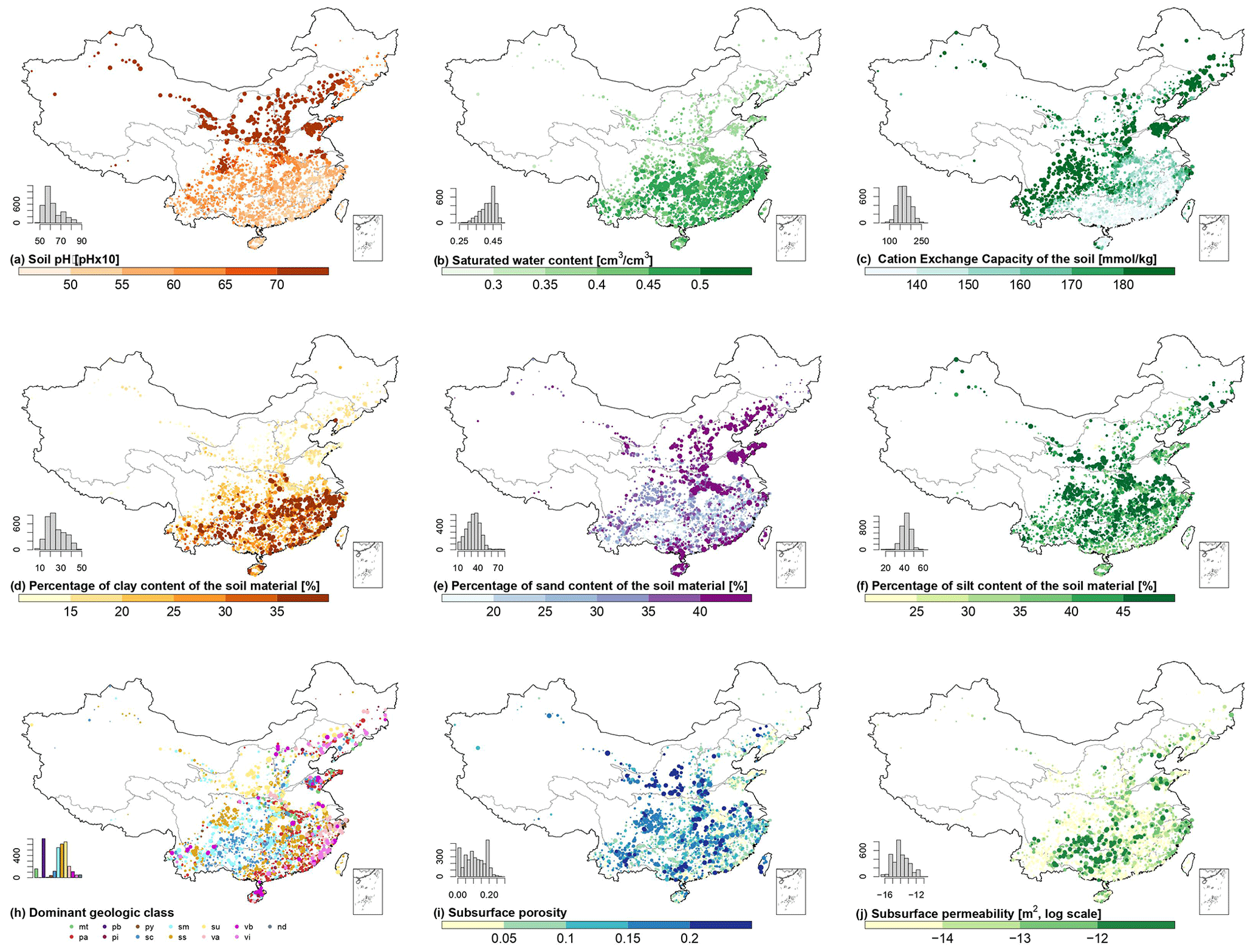
Figure 12Distribution of selected soil and geology characteristics of intermediate catchments and full catchments. Each category's histogram indicates the number of basins (out of 3254). In a histogram, the x axis represents the number of basins, while the y axis represents each subplot's caption. Circle sizes are proportional to catchment areas.
Geology characteristics are described by 19 attributes (i.e., subsurface porosity, permeability, and lithological classes) derived from global lithological map (GLiM; Hartmann and Moosdorf, 2012) and global hydrogeology map (GLHYMPS; Gleeson et al., 2014) datasets (Table S15). The two important parameters for groundwater modeling, e.g., subsurface porosity and permeability, came from GLHYMPS. Subsurface porosity is a measure of the ability of the subsurface to store water, while permeability is a measure of the ability of the rock to transmit fluids. Both of these parameters show a high spatial correlation with GLiM, as hydraulic properties in GLHYMPS are based primarily on lithological classes of GLiM. We computed the catchment-level characteristics by applying an arithmetic mean method for porosity and arithmetic-scale geometric mean method for permeability. The lithological classes were derived from GLiM, which was created by summarizing 92 regional lithological maps and offers three classification levels of detail. In this study, we adopted the first level of GLiM, which has 16 lithological classes. Proportions of each lithological class and the dominant class are documented in our datasets.
There are some limitations with these datasets. Firstly, the GLHYMPS module is primarily useful for analyzing regional scales, i.e., scales larger than 5 km, where the effects of local heterogeneities such as fault zones are negligible (Gleeson et al., 2014). Secondly, GLHYMPS is not adequate for analysis in regions dominated by unsaturated processes such as deeply weathered soils, as it is modeled for saturated conditions (Huscroft et al., 2018). Thirdly, data quality varies depending on location, based on raw regional geological maps available in different resolutions and data qualities. In this study, the resolution of the Chinese raw data sources is slightly lower than that of GLiM (Hao et al., 2021).
The soil pH value is high in northern and northeastern China, and the saturated water content is low in this area (Fig. 12a and b). High values of CEC can be found in central and northeastern China and forested parts on the Qinghai–Tibet Plateau (Fig. 12c). The clay content is low in northern China, while the sand content shows the opposite pattern (Fig. 12d and e). The silt content has a wide predominance pattern in China, particularly in the middle and northeastern parts (Fig. 12f). Moreover, we found that soil characteristics are correlated with other attributes from Res-CN as they are predicted by fusing multisource covariates such as climate and landscape attributes. For example, the soil texture (i.e., sand, silt, and clay contents) shows a similar pattern to the aridity index (Figs. 12e and 10f). SOC has a high correlation value with surface slope (Figs. 12c and 10b, R2 = 0.94). The geology attributes have a clear latitude distribution, and the main lithological classes include acid plutonic rocks (21 % of the catchments), siliciclastic sedimentary (20 %), mixed sedimentary (19 %), and carbonate sedimentary (17 %). Medium subsurface porosity and high permeability are typically in northern and coastal areas surrounding the Bohai Sea with abundant unconsolidated sediments, and high porosity and low permeability are often associated with mixed sedimentary rocks in northern Inner Mongolia, the western Yunnan–Guizhou Plateau, and the southern Qinghai–Tibet Plateau (Fig. 12h, i, and e). Interestingly, high values of subsurface porosity are not necessarily accompanied by high values of permeability, producing a more heterogeneous spatial pattern (Fig. 12h) than that in Fig. 12i. There may be differences in permeability and porosity due to the different rock structures of GLiM (Gleeson et al., 2014).
3.4.5 Anthropogenic activity characteristics
We computed four categories of anthropogenic activities in the catchments, including population count, human footprint, nighttime lights, and road density (Table S16). Population counts were derived from the GPW v4.11 (Gridded Population of the World, Center for International Earth Science Information Network – CIESIN – Columbia University, 2018). This collection produces human population estimates for five years (i.e., 2000, 2005, 2010, 2015, and 2020) at a gridded resolution of 30 arcsec. Human footprint is a measure of human activities that use natural resources on Earth and was extracted from the Global Human Footprint dataset (Venter et al., 2016). This database measures the cumulative environmental impact of indirect and direct human activities in 1993 and 2009, and it was produced from eight inputs: electric infrastructure, population density, built environments, pastures, croplands, roads, railroads, and navigable waterways. Nighttime lights are a measure of human activity intensity and were derived from the DMSP-OLS Nighttime Lights version 4 (Defense Meteorological Program-Operational Line-Scan; Doll, 2008). This database can detect visible and near-infrared emission sources at night and consists of cloud-free composites made using all the available archived DMSP-OLS smooth resolution data at a resolution of 30 arcsec. The “avg_lights_x_pc” in this dataset is used in this study and represents the mean value of cloud-free light detections in the visible band. The road density was obtained from the Global Roads Inventory Project (GRIP; Meijer et al., 2018), providing global raster datasets of road density at a 5 arcmin spatial resolution. Using 60 geospatial datasets on road infrastructure, this inventory gathers, harmonizes, and integrates over 21×106 km of roads by country.
These datasets are subject to some limitations. First, cumulative pressures of human footprint are static through time due to a lack of available data, which would lead to an underestimation of human footprint if those pressures expanded at an above-average rate. Second, some static pressures, like the pollution and invasive species, are not considered in the cumulative pressures of human footprint. Third, the GRIP datasets cannot quantify historic road expansion due to the missing information on the year of construction. Fourth, DMSP-OLS has the blooming effect (i.e., overestimation of lit area) due to the low spatial resolution and the reflectance of light from adjacent waterbodies.
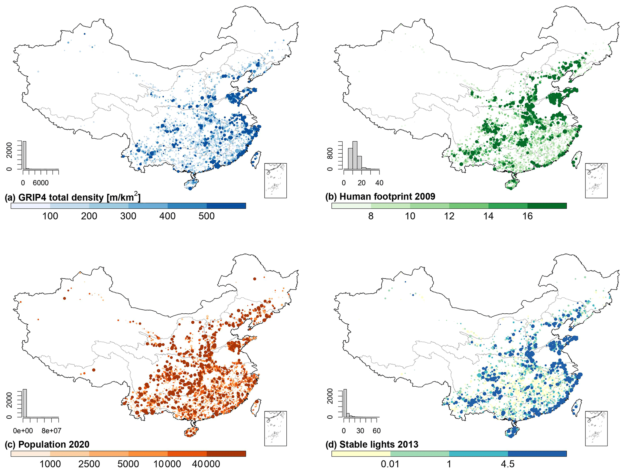
Figure 13Distribution of human activity characteristics of intermediate and full catchments. Each category's histogram indicates the number of basins (out of 3254). In a histogram, the x axis represents the number of basins, while the y axis represents each subplot's caption. Circle sizes are proportional to catchment areas.
Figure 13 illustrates the spatial distribution of four anthropogenic indices in the catchments. Road density, population count, lights, and human footprint show similar patterns, suggesting that intense human activities are distributed in the coastal lines surrounding the East Sea and Bohai Sea, middle China, and northeastern China, and there is almost no human activity in northwestern China due to high elevation and harsh environment.
The Res-CN archive can be found here: https://doi.org/10.5281/zenodo.7664489 (Shen et al., 2022c). It is distributed with a CC-BY license. The files provided are (A) shapefiles; (B) full catchments containing all catchment-level attributes such as climate, topographic, land cover, soil, geological, anthropogenic activities, and time series of meteorological variables; (C) intermediate catchments; (D) reservoir states (i.e., water level, water surface area, evaporation, and storage anomaly); and (E) an information file in English containing more information on RES-CN, as well as validation figures containing the figures depicting the time series of reservoir states and detailed evaluation reports based on in situ data when available. All input datasets are summarized in the Supplement and kindly acknowledged.
All scripts for generating our reservoir datasets are available in the data product.
In this study, we have produced a comprehensive and extensive dataset of reservoir-catchment characteristics in China, Res-CN, which complementarily improved the existing reservoir datasets. We demonstrated that the construction of Res-CN involved a first known effort to construct catchment-level characteristics of reservoirs for our delineated full catchments and intermediate catchments of reservoirs. The 512 static catchment-level attributes for 3254 reservoirs in six categories (i.e., reservoir and catchment body characteristics, topography, climate, soil and geology, land cover and use, and anthropogenic activity characteristics) are included in Res-CN. Additionally, 15 climatic variables were extracted at daily scale, which can drive machine learning models or hydrological models for simulations. Alongside the catchment-level attributes, we produced a significantly enhanced spatial and temporal coverage (e.g., 67 % increase in spatial resolution of water level and 225 % increase in storage anomaly) of water level (data available for 20 % of 3254 reservoirs), water surface area (99 %), storage anomaly (92 %), and evaporation (98 %) by utilizing multiple satellites such as operational satellite altimeters and imagery data. In situ data of 138 reservoirs are employed in this study as a valuable reference for evaluation, thus enhancing our confidence in the data quality and enhancing our understanding of the accuracy of current satellite datasets. We have considered and discussed the deficits, limitations, and uncertainties of Res-CN for further applications.
We envision that Res-CN with its comprehensive and extensive attributes can provide strong support to a wide range of applications and disciplines. Firstly, our two types of catchments along with their catchment-level attributes allow for investigations within individual catchments and interconnected river networks. For example, as illustrated in Fig. 2, users may quantify the relative contributions of upstream reservoirs and local drainage catchment on water quality (e.g., algae contributions and water color) of the downstream reservoir by tracking temperature and nutrient flows from upstream reservoirs and intermediate catchments (e.g., X. Hou et al., 2022; Yang et al., 2022). Besides, water and sediment transfer can also be more accurately simulated in such a spatially explicit context if appropriate approaches are used. Machine learning methods make it possible to predict reservoir storage change at a 1- to 3-month lead from reservoir upstream attributes and time series of reservoir states (Tiwari and Mishra, 2019). Secondly, Res-CN provides thus far the most comprehensive reservoir states in China for assessing impacts of reservoir regulation and dynamics. Tracking the spatiotemporal balance of reservoir evaporative and water storage can provide a basis for local water management in a warming climate (Di Baldassarre et al., 2019). The reservoir operational rules or impacts of reservoir regulation on flow regimes are possibly inferred from reservoir water dynamics in Res-CN (Vu et al., 2022). This is particularly true if the reservoir inflow is also utilized. Recently, the gridded natural runoff provided by Gou et al. (2021) provides exciting opportunities for quantifying human water regulation in combination with Res-CN (Dang et al., 2022; Shin et al., 2020). Thirdly, our extracted catchment-level attributes can contribute to a better understanding of reservoir water amount and water quality changes by spatially incorporating geophysical and anthropogenic characteristics of their upstream catchments and their respective contributions. For example, cropland in reservoir upstream catchments controls the nutrient-driven primary production, while wetland coverage affects dissolved organic material transport downstream, ultimately impacting primary production and CO2 emissions in lakes (Balmer and Downing, 2011; Borges et al., 2022; Maberly et al., 2013). Gradient and altitude in the reservoir geological attributes may affect greenhouse gas emissions and biogeochemistry of a reservoir (Casas-Ruiz et al., 2020). Furthermore, these catchment-level attributes can be used to explore water fluxes and sediment transportation even in reservoirs that have not been sampled. Studies on cascading patterns in reservoir attributes found that each attribute may display a linear function of catchment area, concluding that cascading patterns of each attribute have different implications for dam management (Faucheux et al., 2022). For instance, one study combined knowledge of catchment attributes with economic, climate, and landscape data to inform reservoir removal decisions in California's Central Valley basin (Null et al., 2014). Lastly, carbon dioxide emissions from reservoirs show significant spatial and seasonal variation, highlighting the importance of hydrology in terrestrial–reservoir carbon transfers and the need to consider this effect when plumbing terrestrial carbon budgets. Res-CN also offers exciting opportunities to address changes in reservoir storage that may be linked to carbon dioxide emissions changes.
Although Res-CN presents significant improvements over existing datasets and holds potential for various applications identified above, a few limitations should be acknowledged. Res-CN is generated using GeoDAR v1 shapefiles (Wang et al., 2022) instead of the newly produced datasets by Song et al. (2022), which added an additional nearly 60 000 very small reservoir shapefiles (< 1 km2). As this study aims to provide a comprehensive and extensive dataset of reservoir-catchment characteristics in China for a better understanding of reservoir impacts on hydrological and biochemical cycles, these thousands of very small reservoirs are not included in our study. Meanwhile, it is currently not feasible to generate satellite-based datasets for these small reservoirs due to the limitations of current satellite altimetry missions, which are unable to detect such reservoirs because of the sparsity of their altimetric ground tracks. These additional small reservoirs only account for 8 % of total water capacity in China. Nonetheless, users can freely access our codes to calculate any reservoir attribute for individual applications or other areas, and they can enrich the inventory if new data become available.
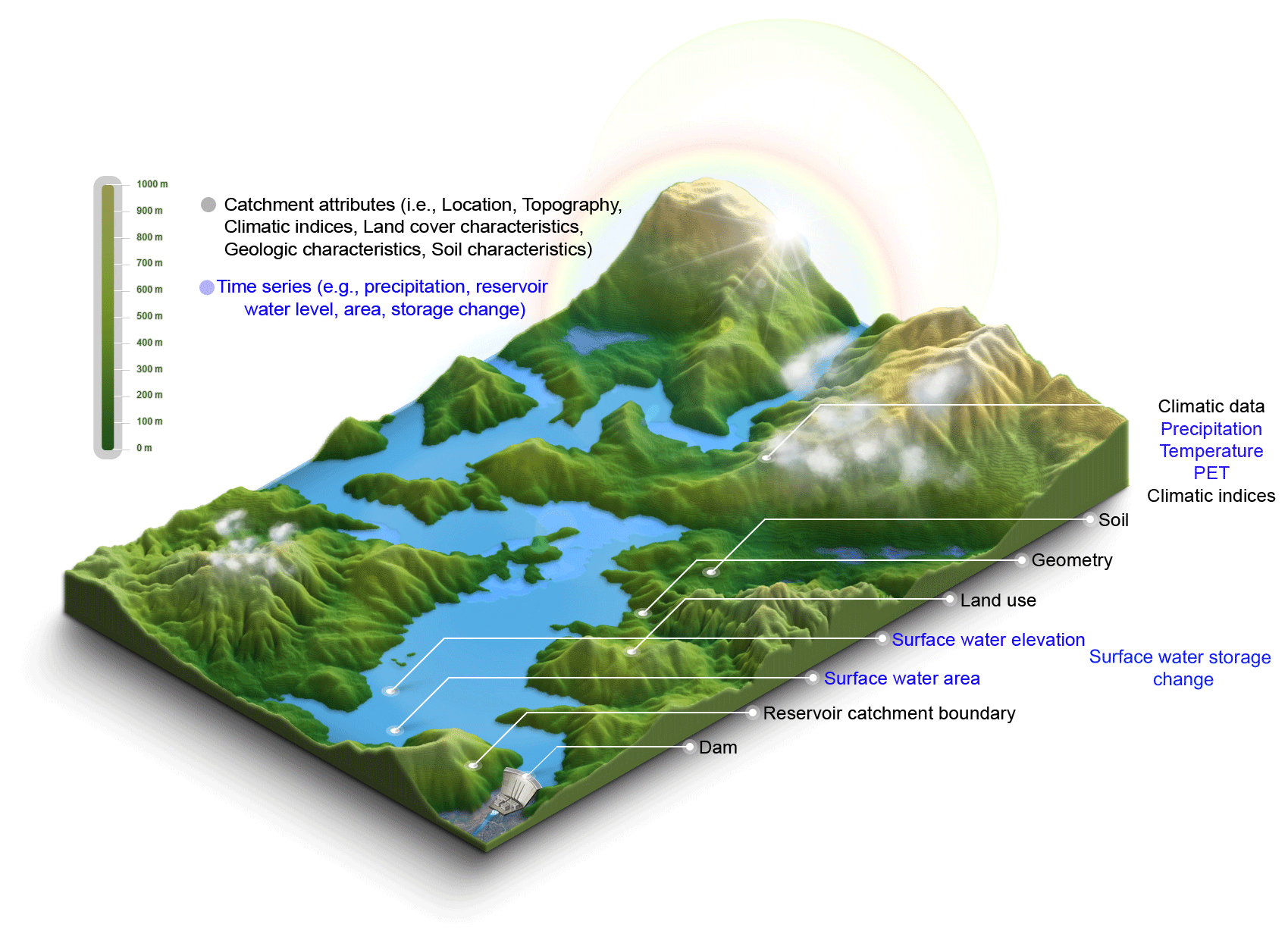
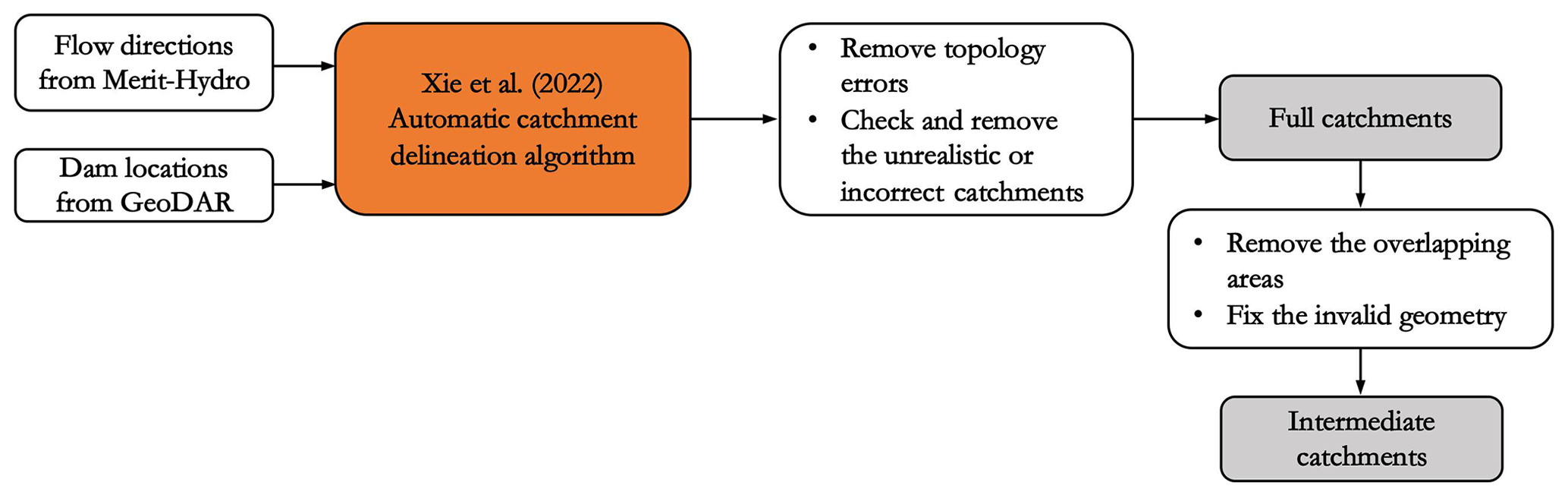
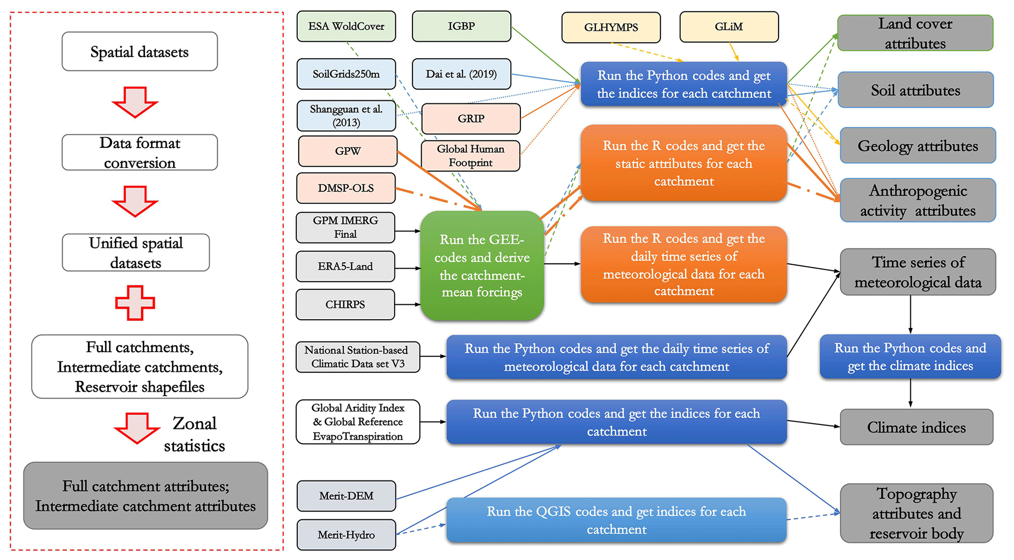
Figure A3Flowchart for generating reservoir upstream catchment-level characteristics. (overview of the methodology in the left panel; we give detailed steps for generating each attribute based on our provided codes. Users can freely access our codes in our Res-CN product.
The Supplement contains many tables, figures, and texts illustrating the methodologies and source datasets for generating Res-CN, as well as detailed evaluations of our Res-CN datasets and all necessary explanations related to this article. The supplement related to this article is available online at: https://doi.org/10.5194/essd-15-2781-2023-supplement.
YS and DY designed the research and initiated the investigation. YS processed the datasets and created the figures. KN extracted data from satellite altimeters. MR and DL reviewed the manuscript. YS wrote and prepared the manuscript with suggestions from co-authors.
The contact author has declared that none of the authors has any competing interests.
Publisher's note: Copernicus Publications remains neutral with regard to jurisdictional claims in published maps and institutional affiliations.
Data from various data centers are acknowledged by the authors. For more acknowledgements, please refer to the Supplement and our datasets. Youjiang Shen also acknowledges the contributions from the EOForChina project. Youjiang Shen is funded by the China Scholarship Council, which is greatly acknowledged.
This research has been supported by the Japan Society for the Promotion of Science (KAKENHI (grant no. 21H05002)).
This paper was edited by Dalei Hao and reviewed by Yadu Pokhrel and two anonymous referees.
Abatzoglou, J. T., Dobrowski, S. Z., Parks, S. A., and Hegewisch, K. C.: TerraClimate, a high-resolution global dataset of monthly climate and climatic water balance from 1958–2015, Sci. Data, 5, 170191, https://doi.org/10.1038/sdata.2017.191, 2018.
Addor, N., Newman, A. J., Mizukami, N., and Clark, M. P.: The CAMELS data set: catchment attributes and meteorology for large-sample studies, Hydrol. Earth Syst. Sci., 21, 5293–5313, https://doi.org/10.5194/hess-21-5293-2017, 2017.
Alvarez-Garreton, C., Mendoza, P. A., Boisier, J. P., Addor, N., Galleguillos, M., Zambrano-Bigiarini, M., Lara, A., Puelma, C., Cortes, G., Garreaud, R., McPhee, J., and Ayala, A.: The CAMELS-CL dataset: catchment attributes and meteorology for large sample studies – Chile dataset, Hydrol. Earth Syst. Sci., 22, 5817–5846, https://doi.org/10.5194/hess-22-5817-2018, 2018.
Balmer, M. B. and Downing, J. A.: Carbon dioxide concentrations in eutrophic lakes: undersaturation implies atmospheric uptake, Inland Waters, 1, 125–132, https://doi.org/10.5268/IW-1.2.366, 2011.
Barbarossa, V., Schmitt, R. J., Huijbregts, M. A., Zarfl, C., King, H., and Schipper, A. M.: Impacts of current and future large dams on the geographic range connectivity of freshwater fish worldwide, P. Natl. Acad. Sci. USA, 117, 3648–3655, 2020.
Birkett, C., Reynolds, C., Beckley, B., and Doorn, B.: From research to operations: the USDA global reservoir and lake monitor, in: Coastal Altimetry, Springer, Berlin, Heidelberg, 19–50, https://doi.org/10.1007/978-3-642-12796-0_2, 2011.
Borges, A. V., Deirmendjian, L., Bouillon, S., Okello, W., Lambert, T., Roland, F. A. E., Razanamahandry, V. F., Voarintsoa, N. R. G., Darchambea, F., Kimirei, I. A., Descy, J.-P., Allen, G. H., and Morana, C.: Greenhouse gas 55 emissions from African lakes are no longer a blind spot, Sci. Adv., 8, eabi8716, https://doi.org/10.1126/sciadv.abi8716, 2022.
Boulange, J., Hanasaki, N., Yamazaki, D., Pokhrel, Y.: Role of dams in reducing global flood exposure under climate change, Nat. Commun., 12, 1–7, https://doi.org/10.1038/s41467-020-20704-0, 2021.
Buccola, N. L., Risley, J. C., and Rounds, S. A.: Simulating future water temperatures in the north Santiam River, Oregon, J. Hydrol., 535, 318–330, https://doi.org/10.1016/j.jhydrol.2016.01.062, 2016.
Busker, T., de Roo, A., Gelati, E., Schwatke, C., Adamovic, M., Bisselink, B., Pekel, J.-F., and Cottam, A.: A global lake and reservoir volume analysis using a surface water dataset and satellite altimetry, Hydrol. Earth Syst. Sci., 23, 669–690, https://doi.org/10.5194/hess-23-669-2019, 2019.
Carpenter, S. R., Stanley, E. H., and Vander Zanden, M. J.: State of the world's freshwater ecosystems: physical, chemical, and biological changes, Annu. Rev. Env. Resour., 36, 75–99, 2011.
Casas-Ruiz, J. P., Hutchins, R. H. S., and del Giorgio, P. A.: Total Aquatic Carbon Emissions Across the Boreal Biome of Queìbec Driven by Watershed Slope, J. Geophys. Res.-Biogeo., 126, e2020JG005863, https://doi.org/10.1029/2020JG005863, 2020.
Chagas, V. B. P., Chaffe, P. L. B., Addor, N., Fan, F. M., Fleischmann, A. S., Paiva, R. C. D., and Siqueira, V. A.: CAMELS-BR: hydrometeorological time series and landscape attributes for 897 catchments in Brazil, Earth Syst. Sci. Data, 12, 2075–2096, https://doi.org/10.5194/essd-12-2075-2020, 2020.
Chaudhari, S., Felfelani, F., Shin, S., and Pokhrel, Y.: Climate and anthropogenic contributions to the desiccation of the second largest saline lake in the twentieth century, J. Hydrol., 560, 342–353, https://doi.org/10.1016/j.jhydrol.2018.03.034, 2018.
Chen, T., Song, C., Fan, C. Cheng, J., Duan, X., Wang, L., Liu, K., Deng, S., and Che, Y.: A comprehensive data set of physical and human-dimensional attributes for China's lake basins, Sci. Data., 9, 519, https://doi.org/10.1038/s41597-022-01649-z, 2022.
Coxon, G., Addor, N., Bloomfield, J. P., Freer, J., Fry, M., Hannaford, J., Howden, N. J. K., Lane, R., Lewis, M., Robinson, E. L., Wagener, T., and Woods, R.: CAMELS-GB: hydrometeorological time series and landscape attributes for 671 catchments in Great Britain, Earth Syst. Sci. Data, 12, 2459–2483, https://doi.org/10.5194/essd-12-2459-2020, 2020.
Crétaux, J.-F., Jelinski, W., Calmant, S., Kouraev, A., Vuglinski, V., Bergé-Nguyen, M., Gennero, M.-C., Nino, F., Del Rio, R. A., Cazenave, A., and Maisongrande, P.: SOLS: a lake database to monitor in the Near Real Time water level and storage variations from remote sensing data, Adv. Space Res., 47, 1497–1507, https://doi.org/10.1016/j.asr.2011.01.004, 2011.
Dai, Y., Xin, Q., Wei, N., Zhang, Y., Shangguan, W., Yuan, H., Zhang, S., Liu, S., and Lu, X.: A global high-resolution data set of soil hydraulic and thermal properties for land surface modeling, J. Adv. Model. Earth Sy., 11, 2996–3023, https://doi.org/10.1029/2019MS001784, 2019.
Dang, H., Pokhrel, Y., Shin, S., Stelly, J., Ahlquist, D., and Du Bui, D.: Hydrologic balance and inundation dynamics of Southeast Asia's largest inland lake altered by hydropower dams in the Mekong River basin, Sci. Total Environ., 831, 154833, https://doi.org/10.1016/j.scitotenv.2022.154833, 2022.
Dang, T. D., Vu, D. T., Chowdhury, A. K., and Galelli, S.: A software package for the representation and optimization of water reservoir operations in the VIC hydrologic model, Environ. Modell. Softw., 126 104673, https://doi.org/10.1016/j.envsoft.2020.104673, 2020.
Di Baldassarre, G., Wanders, N., AghaKouchak, A., Kuil, L., Rangecroft, S., Veldkamp, T. I. E., Garcia, M., van Oel, P. R., Breinl, K., and Van Loon, A. F.: Water shortages worsened by reservoir effects, Nat. Sustain., 1, 617–622, https://doi.org/10.1038/s41893-018-0159-0, 2018.
Didan, K.: MODIS/Terra Vegetation Indices 16-Day L3 Global 250m SIN Grid V061, NASA EOSDIS Land Processes DAAC [data set], https://doi.org/10.5067/MODIS/MOD13Q1.061, 2021.
Doll, C. N.: CIESIN Thematic Guide to Night-Time Light Remote Sensing and Its Applications, Center for International Earth Science Information Network, Palisades, NY, USA, 41 pp., 2008.
Donchyts, G., Baart, F., Winsemius, H., Gorelick, N., Kwadijk, J., and van de Giesen, N.: Earth's surface water change over the past 30 years, Nat. Clim. Change, 6, 810–813, https://doi.org/10.1038/nclimate3111, 2016.
Donchyts, G., Winsemius, H., Baart, F., Dahm, R., Schellekens, J., Gorelick, N., Iceland, C., and Schmeier, S.: High-resolution surface water dynamics in Earth's small and medium-sized reservoirs, Sci. Rep., 12, 13776, https://doi.org/10.1038/s41598-022-17074-6, 2022.
Faucheux, N. M., Sample, A. R., Aldridge, C. A., Norris, D. M., Owens, C., Starnes, V. R., VanderBloemen, S., and Miranda, L. E.: Reservoir attributes display cascading spatial patterns along river basins, Water Resour. Res., 58, e2021WR029910, https://doi.org/10.1029/2021WR029910, 2022.
Galelli, S., Dang, T. D., Ng, J. Y., Chowdhury, A., and Arias, M. E.: Opportunities to curb hydrological alterations via dam re-operation in the Mekong, Nat. Sustain., 5, 1058–1069, https://doi.org/10.1038/s41893-022-00971-Z, 2022.
Gao, H., Birkett, C., and Lettenmaier, D. P.: Global monitoring of large reservoir storage from satellite remote sensing, Water Resour. Res., 48, W09504, https://doi.org/10.1029/2012WR012063, 2012.
Gleeson, T., Moosdorf, N., Hartmann, J., and van Beek, L. P. H.: A glimpse beneath earth's surface: GLobal HYdrogeology MaPS (GLHYMPS) of permeability and porosity, Geophys. Res. Lett., 41, 3891–3898, https://doi.org/10.1002/2014GL059856, 2014.
Gleick, P. H.: The World's Water 2008–2009, Island Press, 79–100, ISBN 9781597265041, 2009.
Gou, J., Miao, C., Samaniego, L., Xiao, M., Wu, J., and Guo, X.: CNRD v1.0: A High-Quality Natural Runoff Dataset for Hydrological and Climate Studies in China, B. Am. Meteorol. Soc., 102, E929–E947, https://doi.org/10.1175/BAMS-D-20-0094.1, 2021.
Gu, L., Chen, J., Yin, J., Slater, L. J., Wang, H. M., Guo, Q., Feng, M., Qin, H., and Zhao, T.: Global Increases in Compound Flood-Hot Extreme Hazards Under Climate Warming, Geophys. Res. Lett., 49, e2022GL097726, https://doi.org/10.1029/2022GL097726, 2022.
Hao, Z., Jin, J., Xia, R., Tian, S., Yang, W., Liu, Q., Zhu, M., Ma, T., Jing, C., and Zhang, Y.: CCAM: China Catchment Attributes and Meteorology dataset, Earth Syst. Sci. Data, 13, 5591–5616, https://doi.org/10.5194/essd-13-5591-2021, 2021.
Hartmann, J. and Moosdorf, N.: The new global lithological map database GLiM: A representation of rock properties at the Earth surface, Geochem. Geophy. Geosy., 13, 1–37, https://doi.org/10.1029/2012GC004370, 2012.
Hengl, T., Mendes de Jesus, J., Heuvelink, G. B., Ruiperez Gonzalez, M., Kilibarda, M., Blagotic ì, A., Shangguan, W., Wright, M. N., Geng, X., and Bauer-Marschallinger, B.: SoilGrids250m: Global gridded soil information based on machine learning, PLOS ONE, 12, e0169748, https://doi.org/10.1371/journal.pone.0169748, 2017.
Horn, B. K. P.: Hill shading and the reflectance map, P. IEEE, 69, 14–47, https://doi.org/10.1109/PROC.1981.11918, 1981.
Hou, J., van Dijk, A. I. J. M., Beck, H. E., Renzullo, L. J., and Wada, Y.: Remotely sensed reservoir water storage dynamics (1984–2015) and the influence of climate variability and management at a global scale, Hydrol. Earth Syst. Sci., 26, 3785–3803, https://doi.org/10.5194/hess-26-3785-2022, 2022.
Hou, X., Feng, L., Dai, Y., Hu, C., Gibson, L., Tang, J., Lee, Z., Wang, Y., Cai, X., Liu, J., Zheng, Y., and Zheng, C.: Global mapping reveals increase in lacustrine algal blooms over the past decade, Nat. Geosci., 15, 130–134, https://doi.org/10.1038/s41561-021-00887-x, 2022.
Huscroft, J., Gleeson, T., Hartmann, J., and Börker, J.: Compiling and Mapping Global Permeability of the Unconsolidated and Consolidated Earth: GLobal HYdrogeology MaPS 2.0 (GLHYMPS 2.0), Geophys. Res. Lett., 45, 1897–1904, https://doi.org/10.1002/2017GL075860, 2018.
Huziy, O., and Sushama, L.: Impact of lake–river connectivity and interflow on the Canadian RCM simulated regional climate and hydrology for Northeast Canada, Clim. Dynam., 48, 709–725, https://doi.org/10.1007/s00382-016-3104-9, 2017.
Khandelwal, A., Karpatne, A., Ravirathinam, P., Ghosh, R., Wei. Z., Dugan, H. A., Hanson, P. C., and Kumar, V.: ReaLSAT, a global dataset of reservoir and lake surface area variations, Sci. Data, 9, 356, https://doi.org/10.1038/s41597-022-01449-5, 2022.
Klein, I., Mayr, S., Gessner, U., Hirner, A., and Kuenzer, C.: Water and hydropower reservoirs: High temporal resolution time series derived from MODIS data to characterize seasonality and variability, Remote Sens. Environ., 253, 112207, https://doi.org/10.1016/j.rse.2020.112207, 2021.
Klingler, C., Schulz, K., and Herrnegger, M.: LamaH-CE: LArge-SaMple DAta for Hydrology and Environmental Sciences for Central Europe, Earth Syst. Sci. Data, 13, 4529–4565, https://doi.org/10.5194/essd-13-4529-2021, 2021.
Lehner, B., Liermann, C. R., Revenga, C., Vörösmarty, C., Fekete, B., Crouzet, P., Döll, P., Endejan, M., Frenken, K., Magome, J., Nilsson, C., Robertson, J. C., Rödel, R., Sindorf, N., and Wisseret, D.: High-resolution mapping of the world's reservoirs and dams for sustainable river-flow management, Front. Ecol. Environ., 9, 494–502, https://doi.org/10.1890/100125, 2011.
Lehner, B., Messager, M. L., Korver, M. C., and Linke, S.: Global hydro-environmental lake characteristics at high spatial resolution, Sci. Data, 9, 351, https://doi.org/10.1038/s41597-022-01425-z, 2022.
Li, R., Xiong, L., Xiong, B., Li, Y., Xu, Q., Cheng, L., and Xu, C.-Y.: Investigating the downstream sediment load change by an index coupling effective rainfall information with reservoir sediment trapping capacity, J. Hydrol., 590, 125200, https://doi.org/10.1016/j.jhydrol.2020.125200, 2020.
Liu, J., Jiang, L., Zhang, X., Druce, D., Kittel, C. M. M., Tøttrup, C., and Bauer-Gottwein, P.: Impacts of water resources management on land water storage in the North China Plain: Insights from multi-mission earth observations, J. Hydrol., 603, 126933, https://doi.org/10.1016/j.jhydrol.2021.126933, 2021.
Liu, J., Fang, P., Que, Y., Zhu, L.-J., Duan, Z., Tang, G., Liu, P., Ji, M., and Liu, Y.: A dataset of lake-catchment characteristics for the Tibetan Plateau, Earth Syst. Sci. Data, 14, 3791–3805, https://doi.org/10.5194/essd-14-3791-2022, 2022.
Maavara, T., Chen, Q., Van Meter, K., Brown, L. E., Zhang, J., Ni, J., and Zarfl, C.: River dam impacts on biogeochemical cycling, Nat. Rev. Earth Environ., 1, 103–116, 2020.
Maberly, S., Barker, P., Stott, A., and De Ville, M. M.: Catchment productivity controls CO2 emissions from lakes, Nat. Clim. Change, 3, 391–394, https://doi.org/10.1038/nclimate1748, 2013.
Markert, K. N., Pulla, S. T., Lee, H., Markert, A. M., Anderson, E. R., Okeowo, M. A., and Limaye, A. S.: AltEx: An open source web application and toolkit for accessing and exploring altimetry datasets, Environ. Modell. Softw., 117, 164–175, https://doi.org/10.1016/j.envsoft.2019.03.021, 2019.
Markert, K. N., Markert, A. M., Mayer, T., Nauman, C., Haag, A., Poortinga, A., Bhandari, B., Thwal, N. S., Kunlamai, T., Chishtie, F., Kwant, M., Phongsapan, K., Clinton, N., Towashiraporn, P., and Saah, D.: Comparing sentinel-1 surface water mapping algorithms and radiometric terrain correction processing in southeast asia utilizing google earth engine, Remote Sens.-Basel, 12, 2469, https://doi.org/10.3390/rs12152469, 2020.
Marx, A., Dusek, J., Jankovec, J., Sanda, M., Vogel, T., van Geldern, R., Hartmann, J., and Barth, J. A. C.: A review of CO2 and associated carbon dynamics in headwater streams: A global perspective, Rev. Geophys., 55, 560–585, https://doi.org/10.1002/2016RG000547, 2017.
Meijer, J., Huijbregts, M., Schotten, K., and Schipper, A.: Global patterns of current and future road infrastructure, Environ. Res. Lett., 13, 064006, https://doi.org/10.1088/1748-9326/aabd42, 2018.
Messager, M. L., Lehner, B., Grill, G., Nedeva, I., and Schmitt, O.: Estimating the volume and age of water stored in global lakes using a geo-statistical approach, Nat. Commun., 7, 13603, https://doi.org/10.1038/ncomms13603, 2016.
MWR: Hydrologic Data Yearbook, Ministry of Water Resources (MWR), ISBN 9771009737167, 2016.
Myneni, R., Knyazikhin, Y., and Park, T.: MCD15A3H MODIS/Terra+Aqua Leaf Area Index/FPAR 4-day L4 Global 500m SIN Grid V006 [data set], NASA EOSDIS Land Processes DAAC, https://doi.org/10.5067/MODIS/MCD15A3H.006, 2015.
NASA JPL: NASA Shuttle Radar Topography Mission Water Body Data Shapefiles & Raster Files, NASA EOSDIS Land Processes DAAC [data set], https://doi.org/10.5067/MEaSUREs/SRTM/SRTMSWBD.003, 2013.
Ngor, P. B., Legendre, P., Oberdorff, T., and Lek, S.: Flow alterations by dams shaped fish assemblage dynamics in the complex Mekong-3S river system, Ecol. Indic., 88, 103–114, https://doi.org/10.1016/j.ecolind.2018.01.023, 2018.
Nielsen, K., Stenseng, L., Andersen, O. B., Villadsen, H., and Knudsen, P.: Validation of CryoSat-2 SAR mode based lake levels, Remote Sens. Environ., 171, 162–170, https://doi.org/10.1016/j.rse.2015.10.023, 2015.
Null, S. E., Medellín-Azura, J., Escriva-Bou, A., Lent, M., and Lund, J. R.: Optimizing the dammed: Water supply losses and fish habitat gains from dam removal in California, J. Environ. Manage., 136, 121–131, https://doi.org/10.1016/j.jenvman.2014.01.024, 2014.
Papa, F., Prigent, C., Aires, F., Jimenez, C., Rossow, W. B., and Matthews, E.: Interannual variability of surface water extent at the global scale, 1993–2004, J. Geophys. Res.-Atmos., 115, D12111, https://doi.org/10.1029/2009JD012674, 2010.
Pavlis, N. K., Holmes, S. A., Kenyon, S. C., and Factor, J. K.: The development and evaluation of the Earth Gravitational Model 2008 (EGM2008), J. Geophys. Res.-Sol. Ea., 117, B04406, https://doi.org/10.1029/2011JB008916, 2012.
Running, S. and Zhao, M.: MODIS/Terra Net Primary Production Gap-Filled Yearly L4 Global 500m SIN Grid V061, NASA EOSDIS Land Processes DAAC [data set], https://doi.org/10.5067/MODIS/MOD17A3HGF.061, 2021.
Running, S., Mu, Q., and Zhao, M.: MODIS/Terra Gross Primary Productivity 8-Day L4 Global 500m SIN Grid V061, NASA EOSDIS Land Processes DAAC [data set], https://doi.org/10.5067/MODIS/MOD17A2H.061, 2021.
Schwatke, C., Dettmering, D., Bosch, W., and Seitz, F.: DAHITI – an innovative approach for estimating water level time series over inland waters using multi-mission satellite altimetry, Hydrol. Earth Syst. Sci., 19, 4345–4364, https://doi.org/10.5194/hess-19-4345-2015, 2015.
Shangguan, W., Dai, Y., Liu, B., Zhu, A., Duan, Q., Wu, L., Ji, D., Ye, A., Yuan, H., and Zhang, Q.: A China data set of soil prop- erties for land surface modeling, J. Adv. Model. Earth Sy., 5, 212–224, https://doi.org/10.1002/jame.20026, 2013.
Shangguan, W., Dai, Y., Duan, Q., Liu, B., and Yuan, H.: A global soil data set for earth system modeling, J. Adv. Model. Earth Sy., 6, 249–263, https://doi.org/10.1002/2013MS000293, 2014.
Shen, Y., Liu, D., Jiang, L., Nielsen, K., Yin, J., Liu, J., and Bauer-Gottwein, P.: High-resolution water level and storage variation datasets for 338 reservoirs in China during 2010–2021, Earth Syst. Sci. Data, 14, 5671–5694, https://doi.org/10.5194/essd-14-5671-2022, 2022a.
Shen, Y., Liu, D., Jiang, L., Tøttrup, C., Druce, D., Yin, J., Nielsen, K., Bauer-Gottwein, P., Wang, J., and Zhao X.: Estimating reservoir release using multi-source satellite datasets and hydrological modeling techniques, Remote Sens.-Basel, 14, 815, https://doi.org/10.3390/rs14040815, 2022b.
Shen, Y., Nielsen, K., Revel, M., Liu, D., and Yamazaki, D.: A dataset for reservoir-catchment characteristics for 3254 Chinese reservoirs, i.e., Res-CN, Zenodo [data set], https://doi.org/10.5281/zenodo.7664489, 2022c.
Shin, S., Pokhrel, Y., Yamazaki, D., Huang, X., Torbick, N., Qi, J., Pattanakiat, S., Ngo-Duc, T., and Nguyen, T. D.: High resolution modeling of river-floodplain-reservoir inundation dynamics in the Mekong River Basin, Water Resour. Res., 56, e2019WR026449, https://doi.org/10.1029/2019wr026449, 2020.
Song, C., Fan, C., Zhu, J., Wang, J., Sheng, Y., Liu, K., Chen, T., Zhan, P., Luo, S., Yuan, C., and Ke, L.: A comprehensive geospatial database of nearly 100 000 reservoirs in China, Earth Syst. Sci. Data, 14, 4017–4034, https://doi.org/10.5194/essd-14-4017-2022, 2022.
Soranno, P. A., Cheruvelil, K. S., Webster, K. E., Bremigan, M. T., Wagner, T., and Stow, C. A.: Using landscape limnology to classify freshwater ecosystems for multi-ecosystem management and conservation, Bioscience, 60, 440–454, https://doi.org/10.1525/bio.2010.60.6.8, 2010.
Stieglitz, M., Shaman, J., McNamara, J., Engel, V., Shanley, J., and Kling, G. W.: An approach to understanding hydrologic connectivity on the hillslope and the implications for nutrient transport, Global Biogeochem. Cy., 17, 1105, https://doi.org/10.1029/2003GB002041, 2003.
Subramanya, K.: Engineering Hydrology, 4e, McGraw Hill Education Private Limited P-24, Green Park Extension, New Delhi, India, 2013.
Tian, W., Liu, X., Wang, K., Bai, P., and Liu, C.: Estimation of reservoir evaporation losses for China, J. Hydrol., 596, 126142, https://doi.org/10.1016/j.jhydrol.2021.126142, 2021.
Tian, W., Liu, X., Wang, K., Bai, P., Liu, C., and Liang, X.: Estimation of global reservoir evaporation losses, J. Hydrol., 607, 127524, https://doi.org/10.1016/j.jhydrol.2022.127524, 2022.
Tiwari, A. D. and Mishra, V.: Prediction of reservoir storage anomalies in India, J. Geophys. Res.-Atmos., 124, 3822–3838, https://doi.org/10.1029/2019JD030525, 2019.
Tourian, M. J., Elmi, O., Shafaghi, Y., Behnia, S., Saemian, P., Schlesinger, R., and Sneeuw, N.: HydroSat: geometric quantities of the global water cycle from geodetic satellites, Earth Syst. Sci. Data, 14, 2463–2486, https://doi.org/10.5194/essd-14-2463-2022, 2022.
Tortini, R., Noujdina, N., Yeo, S., Ricko, M., Birkett, C. M., Khandelwal, A., Kumar, V., Marlier, M. E., and Lettenmaier, D. P.: Satellite-based remote sensing data set of global surface water storage change from 1992 to 2018, Earth Syst. Sci. Data, 12, 1141–1151, https://doi.org/10.5194/essd-12-1141-2020, 2020.
Venter, O., Sanderson, E. W., Magrach, A., Allan, J. R., Beher, J., Jones, K. R., Possingham, H. P., Laurance, W. F., Wood, P., Fekete, B. M., Levy, M. A., and Watson, J. E. M.: Global terrestrial Human Footprint maps for 1993 and 2009, Sci. Data, 3, 160067, https://doi.org/10.1038/sdata.2016.67, 2016.
Vu, D. T., Dang, T. D., Galelli, S., and Hossain, F.: Satellite observations reveal 13 years of reservoir filling strategies, operating rules, and hydrological alterations in the Upper Mekong River basin, Hydrol. Earth Syst. Sci., 26, 2345–2364, https://doi.org/10.5194/hess-26-2345-2022, 2022.
Wang, J., Walter, B. A., Yao, F., Song, C., Ding, M., Maroof, A. S., Zhu, J., Fan, C., McAlister, J. M., Sikder, S., Sheng, Y., Allen, G. H., Crétaux, J.-F., and Wada, Y.: GeoDAR: georeferenced global dams and reservoirs dataset for bridging attributes and geolocations, Earth Syst. Sci. Data, 14, 1869–1899, https://doi.org/10.5194/essd-14-1869-2022, 2022.
Wang, X., Xiao, X., Zou, Z. Dong, J., Qin, Y., Doughty, R. B., Menarguez, M. A., Chen, B., Wang, J., Ye, H., Ma, J., Zhong, Q., Zhao, B., and Li. B.: Gainers and losers of surface and terrestrial water resources in China during 1989–2016, Nat. Commun., 11, 3471, https://doi.org/10.1038/s41467-020-17103-w, 2020.
Wilson, A. M. and Jetz, W.: Remotely sensed high-resolution global cloud dynamics for predicting ecosystem and biodiversity distributions, PLOS Biol., 14, e1002415, https://doi.org/10.1371/journal.pbio.1002415, 2016.
Xie, J., Liu, X., Bai, P., and Liu, C.: Rapid watershed delineation using an automatic outlet relocation algorithm, Water Resour. Res., 58, e2021WR031129, https://doi.org/10.1029/2021WR031129, 2022.
Yamazaki, D, Ikeshima, D, Tawatari, R, Yamaguchi, T., O'Loughlin, F., Neal, J. C., Sampson, C. C., Kanae, S., and Bates, P. D.: A high-accuracy map of global terrain elevations, Geophys. Res. Lett., 44, 5844–5853, https://doi.org/10.1002/2017GL072874, 2017.
Yamazaki, D., Ikeshima, D., Sosa, J., Bates, P. D., Allen, G. H., and Pavelsky, T. M.: MERIT Hydro: A high-resolution global hydrography map based on latest topography dataset, Water Resour. Res., 55, 5053–5073, https://doi.org/10.1029/2019WR024873, 2019.
Yang, X., O'Reilly, C. M., Gardner, J. R., Ross, M. R. V., Topp, S. N., Wang, J., and Pavelsky, T. M.: The color of Earth's lakes, Geophys. Res. Lett., 49, e2022GL098925, https://doi.org/10.1029/2022GL098925, 2022.
Zanaga, D., Van De Kerchove, R., De Keersmaecker, W., Souverijns, N., Brockmann, C., Quast, R., Wevers, J., Grosu, A., Paccini, A., Vergnaud, S., Cartus, O., Santoro, M., Fritz, S., Georgieva, I., Lesiv, M., Carter, S., Herold, M., Li, Linlin, Tsendbazar, N. E., Ramoino, F., and Arino, O.: ESA WorldCover 10 m 2020 v100, Zenodo, https://doi.org/10.5281/zenodo.5571936, 2021.
Zeng, X.: Global vegetation root distribution for land modeling, J. Hydrometeorol., 2, 525–530, 2001.
Zhang, X., Jiang, L., Kittel, C. M. M., Yao, Z., Nielsen, K., Liu, Z., Wang, R., Liu, J., Andersen, O. B., and Bauer-Gottwein, P.: On the pertormance of Sentinel-3 altimetry over new reservoirs: Approaches to determine onboard a prior elevation, Geophys. Res. Lett., 47, e2020GL088770, https://doi.org/10.1029/2020GL088770, 2020.
Zhao, G. and Gao, H.: Automatic Correction of Contaminated Images for Assessment of Reservoir Surface Area Dynamics, Geophys. Res. Lett., 45, 6092–6099, https://doi.org/10.1029/2018GL078343, 2018.
Zhao, G. and Gao, H.: Estimating reservoir evaporation losses for the United States: Fusing remote sensing and modeling approaches, Remote Sens. Environ., 226, 109–124, https://doi.org/10.1016/j.rse.2019.03.015, 2019.
Zhao, G., Li, Y., Zhou, L., and Gao, H.: Evaporative water loss of 1.42 million global lakes. Nat. Commun., 13, 3686, https://doi.org/10.1038/s41467-022-31125-6, 2022.
Zhong, R., Zhao, T., and Chen, X.: Hydrological model calibration for dammed basins using satellite altimetry information, Water Resour. Res., 56, e2020WR027442, https://doi.org/10.1029/2020WR027442, 2020.
Zomer, R. J., Xu, J., and Trabucco, A.: Version 3 of the Global Aridity Index and Potential Evapotranspiration Database, Sci. Data, 9, 409, https://doi.org/10.1038/s41597-022-01493-1, 2022.