the Creative Commons Attribution 4.0 License.
the Creative Commons Attribution 4.0 License.
 | 24 Mar 2023
DL-RMD: a geophysically constrained electromagnetic resistivity model database (RMD) for deep learning (DL) applications
Muhammad Rizwan Asif
Nikolaj Foged
Thue Bording
Jakob Juul Larsen
Anders Vest Christiansen
Deep learning (DL) algorithms have shown incredible potential in many applications. The success of these data-hungry methods is largely associated with the availability of large-scale datasets, as millions of observations are often required to achieve acceptable performance levels. Recently, there has been an increased interest in applying deep learning methods to geophysical applications where electromagnetic methods are used to map the subsurface geology by observing variations in the electrical resistivity of the subsurface materials. To date, there are no standardized datasets for electromagnetic methods, which hinders the progress, evaluation, benchmarking, and evolution of deep learning algorithms due to data inconsistency. Therefore, we present a large-scale electrical resistivity model database (RMD) with a wide variety of geologically plausible and geophysically resolvable subsurface structures for the commonly deployed ground-based and airborne electromagnetic systems. Potentially, the presented database can be used to build surrogate models of well-known processes and to aid in labour-intensive tasks. The geophysically constrained property of this database will not only achieve enhanced performance and improved generalization but, more importantly, incorporate consistency and credibility into deep learning models. We show the effectiveness of the presented database by surrogating the forward-modelling process, and we urge the geophysical community interested in deep learning for electromagnetic methods to utilize the presented database. The dataset is publicly available at https://doi.org/10.5281/zenodo.7260886 (Asif et al., 2022a).
- Article
(1402 KB) - Full-text XML
- BibTeX
- EndNote


Recent years have witnessed the success of many deep learning (DL) applications. Although DL emerged in 1982 in the form of neural networks (Hopfield, 1982), it started to gain attention in 2012 due to its notable performance for image classification tasks (Krizhevsky et al., 2017, 2012). Since then, it has been applied successfully to many applications including object detection (Asif et al., 2019; Redmon et al., 2016; Ren et al., 2015), image super-resolution (Dong et al., 2016; Zhang et al., 2018), speech recognition (Zhang et al., 2017), and stock market predictions (Pang et al., 2020). The revival of DL was mainly influenced by the availability of cheap computing resources, deeper network architectures, and large-scale publicly available datasets. Deeper network architectures and an increased number of samples in the training datasets are key factors for improved performance and better generalization of DL models (Wang et al., 2016).
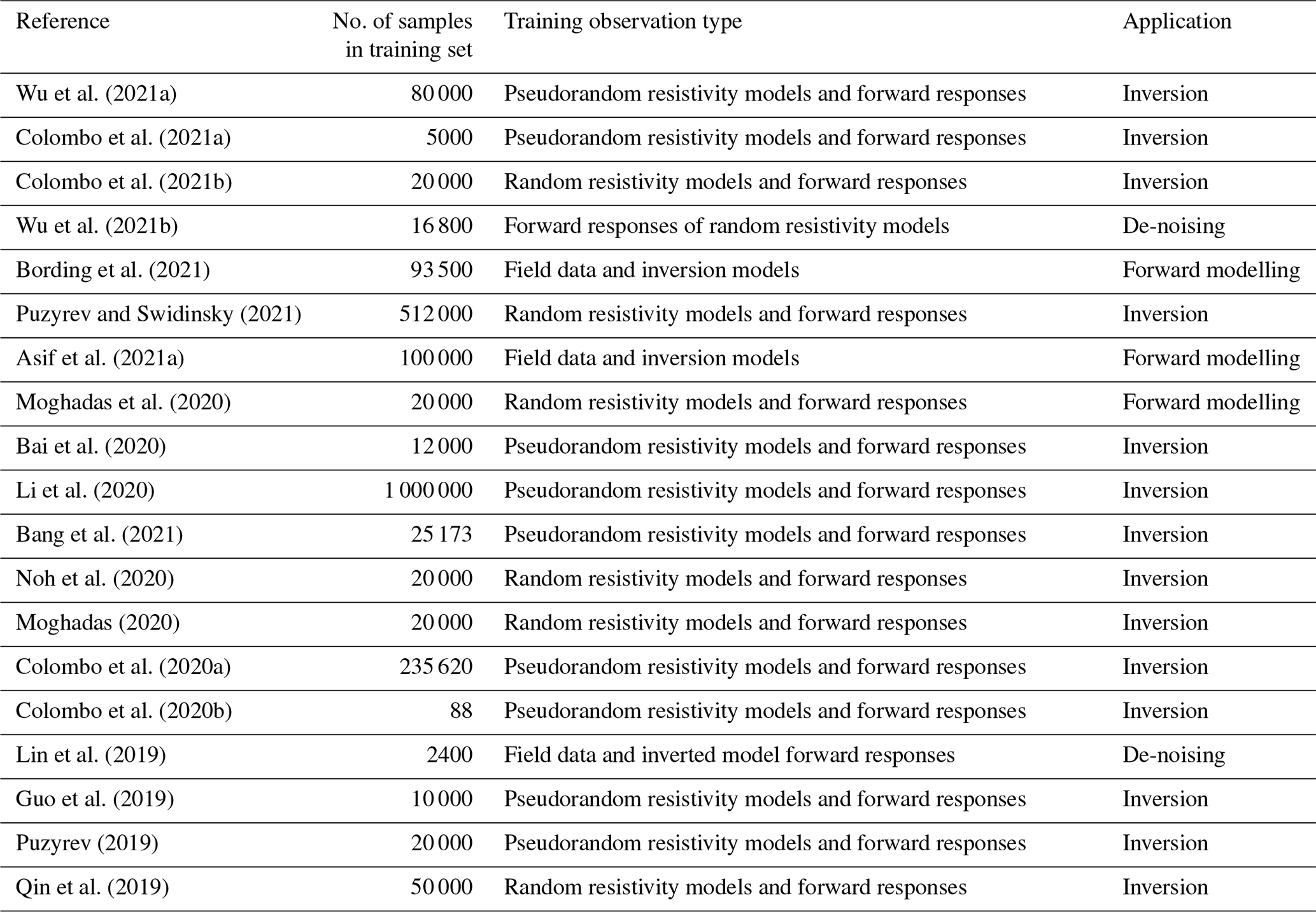
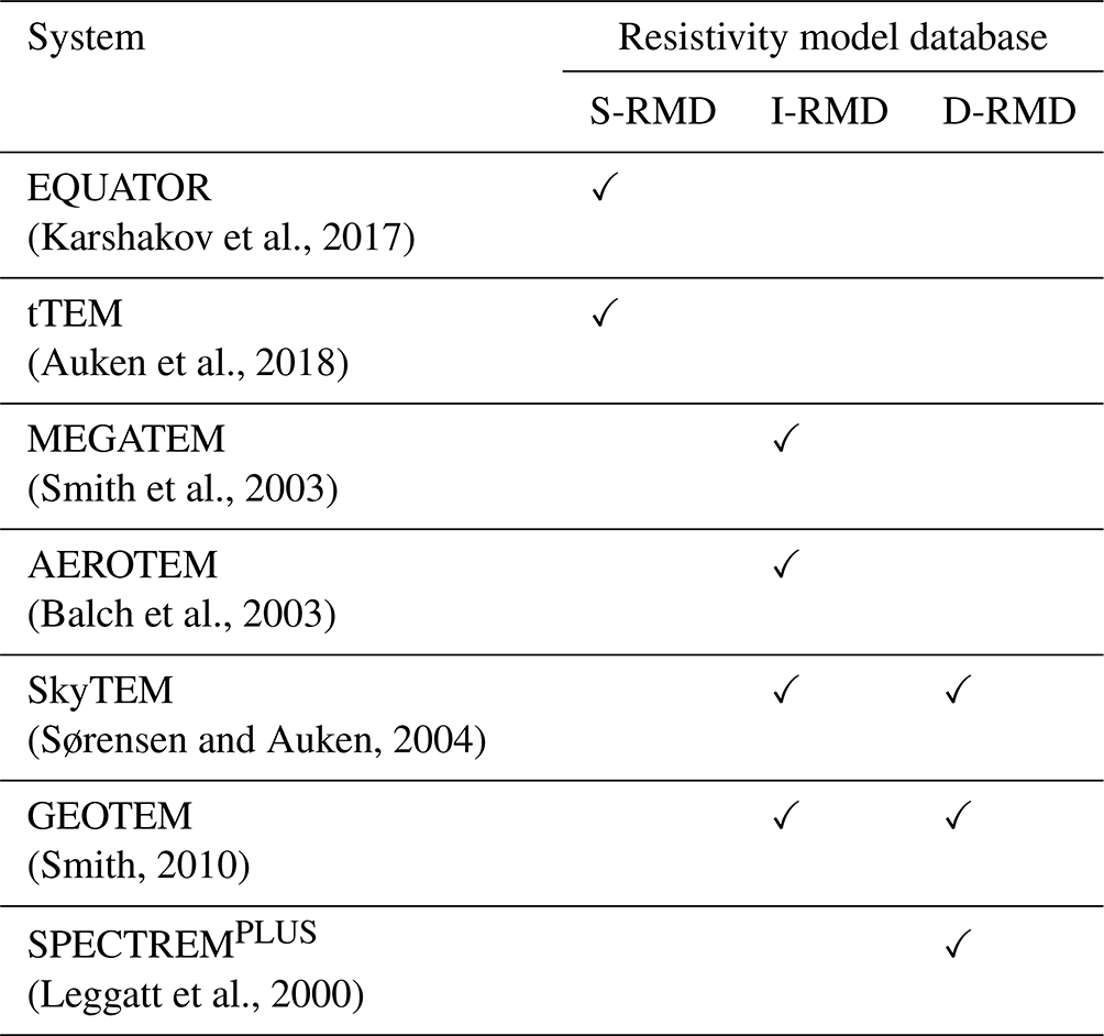
Geophysics is a branch of earth sciences, and geophysical methods are often used to infer information about the subsurface geology by mapping physical properties. The integration of neural networks in geophysics started several decades ago and has covered many domains of geophysics (Baan and Jutten, 2000; Dramsch, 2020), including seismic (Röth and Tarantola, 1994; Zhang et al., 2020), magneto-telluric (Conway et al., 2019; Liu et al., 2020; Zhang and Paulson, 1997), geo-mechanical (Feng and Seto, 1998; Khatibi and Aghajanpour, 2020), and electromagnetic domains (Birken and Poulton, 1999; Birken et al., 1999; Bording et al., 2021; Kwan et al., 2015; Poulton et al., 1992; Zhu et al., 2012). Interestingly, the last few years have seen a significant increase in interest in applying DL to electromagnetic (EM) methods (see Table 1), where the artificially generated EM fields are used to map variations in the electrical resistivity properties of the subsurface. For more details regarding the EM methods, readers are referred to the literature (e.g. Kirsch, 2006). The increasing interest in applying DL to EM methods is mainly influenced by the increased ability of the EM methods to collect huge datasets in short amounts of time, which make the subsequent processes extremely laborious and time consuming. Therefore, a DL method could be beneficial in surrogating well-known EM processes, e.g. forward modelling where the propagation of the EM fields is simulated, resulting in the forward responses (Xue et al., 2020), and inverse modelling (inversion) where the electrical resistivity properties of the subsurface are deduced from observed EM data (Zhdanov, 2015). DL methods can also assist with manual tasks, which may require considerable time when performed manually, such as anomaly detection in EM data. Further opportunities may lie in other tasks, e.g. data de-noising.
To apply a DL algorithm to EM methods for various applications, subsurface resistivity models and/or the corresponding EM responses are often required. To achieve optimal performance, a DL method should be trained on a large number of geologically realistic subsurface models. Evident from Table 1, the recently developed DL methods either use subsurface resistivity models acquired from field data or generate the models randomly or in a pseudorandom manner for training. However, a method trained on random models, where the resistivity of each geological layer is chosen from a probability distribution, would not result in optimal performance, as many of the training samples would be geologically unrealistic. A good solution is to use either resistivity models inverted from field data or pseudorandom resistivity models where the resistivity of the training models is based on some prior geological information to reflect various characteristics of field data (Bai et al., 2020). However, a DL method trained on such training samples would only be effective for specific geological conditions and would result in an unsatisfactory performance for significantly different geological settings (Bording et al., 2021), as bias in the training data can affect generalizability substantially. Additionally, the unavailability of a standard benchmark database hinders the progress, evaluation, benchmarking, and evolution of DL algorithms due to data inconsistency (Bergen et al., 2019; Reichstein et al., 2019).
Table 1Recent publications (2019–2021) of DL applications in EM which show the number of training samples and type of training dataset (random, pseudorandom, or field data).
To have an inclusive DL solution for various applications in EM, we present a physics-driven large-scale model database (∼ 1 million models) of geologically plausible and EM-resolvable 1-D subsurface resistivity models spanning the resistivity range from 1 to 2000 Ωm and to a depth of 500 m. This model database is suitable for ground-based and airborne EM systems in a DL context. We use broad-banded von Kármán covariance functions to generate geologically constrained resistivity models. Geophysical constraints are imposed by calculating the EM forward data of the initial resistivity models followed by inversion of the EM forward data to obtain the final resistivity models. This allows us to create a comprehensive resistivity model database (RMD) that may not only improve performance and generalization but also incorporate consistency and reliability into the DL models. We believe that the presented RMD will be a valuable resource to accelerate the inter- and trans-disciplinary research of earth and data sciences. The presented DL-RMD will also provide uniformity in training and benchmarking for DL methods in EM. Therefore, we urge the geophysical community interested in DL for EM methods to use the DL-RMD.
The rest of this paper is organized as follows. Section 2 describes the general methodology of generating the subsurface resistivity models, while specific settings for the DL-RMD for the three EM system categories are specified in Sect. 3. Section 4 provides details for training a DL method to surrogate the forward-modelling problem and shows the effectiveness of the DL-RMD. Discussion, code and data availability, and concluding remarks are given in Sects. 5, 6, and 7, respectively.
Geological processes do not result in random structures, nor are the subsurface resistivity structures random, as some spatial correlation is generally present (Tacher et al., 2006). Therefore, it is reasonable that the training of a DL method is based on subsurface structures that are geologically plausible and, in an EM context, overall resolvable by the EM method. Additionally, the scale of the resistivity structure in the models should reflect the resolution capability of the EM methods, as training a DL method to resolve structures that are not evident in the input data is not possible. EM methods are diffusive methods with significantly decreasing resolution with depth, and the electrical conductivity contrast plays an important role for the resolution capability; hence, a metric number for a given EM method's resolution capability and the depth of investigation cannot be given.
To obtain geologically realistic models, we use the broad-banded von Kármán covariance functions (Møller et al., 2001) to generate geologically plausible models (von Kármán models). The suite of von Kármán models consists of fine geological structures and contain some resistivity variations and patterns that are unlikely to be resolved, due to the resolution limitation of the EM method. To replicate the resolution capability of the EM method, we generate EM forward responses of the initially over-detailed von Kármán models and invert these forward responses to obtain the final resistivity models. Since we aim at generating 1-D resistivity models, we are only concerned about the resistivity (ρ) variations in the vertical direction (z) from surface to some depth in our model generation.
Initially, we base the spatial variation character of (z, log 10(ρ)) for our von Kármán models on the broad-banded von Kármán covariance functions (Christiansen and Auken, 2003; Møller et al., 2001).
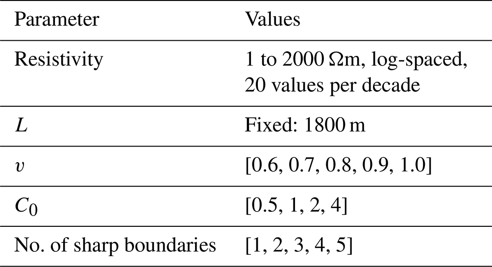
where A becomes the amplitude of the logarithmic resistivity, C0 is a scaling constant, z is the spatial (vertical) distance, L characterizes the maximum correlation length accounted for, and Kν is the modified Bessel function of the second kind and order ν. In the model generation, L is fixed to a high number (1800 m) which gives us strong correlation for z≪L (Maurer et al., 1998). By using combinations of ν, C0, and resistivity and compiling several realizations of the stochastic von Kármán process, we generate a variety of resistivity models on multiple scales. Table 2 summarizes the L, ν, C0, and resistivity values used.
Table 2Parameters used in all combinations to generate the initial von Kármán resistivity models.
Examples of this are shown in Fig. 1a–c where the von Kármán models (in black curves) are generated with a combination of the extreme values of ν and C0 for an initial resistivity value of 30 Ωm. Low ν and high C0 produce models with fine- and large-scale variations (Fig. 1a), while high ν and high C0 values produce a relatively smooth model (Fig. 1b) but still with resistivity variations spanning 2–3 decades of resistivity. The combination of low ν and C0 values ensures that the simple and close-to-half-space models are also represented (Fig. 1c).
Sharp layering in the subsurface is plausible, and large resistivity amplitudes and short correlation lengths in the von Kármán functions will form layering in the models. To include more models with a sharp layering, we stitch 2–6 randomly selected depth intervals of the initially generated von Kármán models from a uniform distribution. An example of a stitched model is shown in Fig. 1d. These stitched models also ensure that different combinations of ν and C0 are represented within one model.
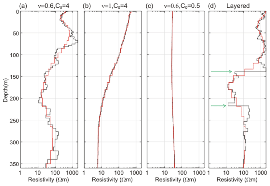
Figure 1Examples of von Kármán models and the result after the forward and inversion process, where black curves show von Kármán models (re-discretized to 90 layers), and the red curve shows the final model. Panels (a) to (c) are for the combination of ν and C0 stated in the title; panel (d) is for a stitched, layered model (green arrows mark the imposed sharp layer boundaries). The red curves show the obtained model from inversion of the forward response of the black model.
Prior to the EM forward calculation, the von Kármán models are re-discretized to 90 layers for faster forward computation and easier handling. The top-layer thickness and depth to the last layer boundary for the re-discretized layers are detailed in Table 3 for three generic EM systems with different depths of investigations (see Sect. 3 for further details). For the forward calculation, the geometric mean of the last 5 m of the re-discretized von Kármán models is assigned to the last model layer that continues to infinite depth. In order to avoid making assumptions on the acquisition conditions, on the specific instrument setups, etc., the calculated forward data are pragmatically assigned a uniform uncertainty of 5 % to take noise into account and are inverted with a 30-layer model with a minimum structure (smooth) regularization scheme (Viezzoli et al., 2008). The layer thicknesses for the 30-layer models are fixed, and they are listed in Table 3. The red model curves in Fig. 1 represent the resistivity models after the forward and inversion process and represent the models that enter the DL-RMD. As seen from Fig. 1, the von Kármán models hold structures that are not resolved by the inverted resistivity models, so the models obtained after the forward and inversion process result in structures resolvable by the EM method. A total of ∼ 95 % of the inverted resistivity models explain (fit) the forward data within the assumed data uncertainty. In other words, the inverted models are explaining the more complex von Kármán models to a very high degree.
The forward and inverse modelling is carried out for three different generic time-domain EM (TEM) systems spanning different depth ranges using the AarhusInv modelling code (Auken et al., 2015). The specific DL-RMD settings for different TEM systems are summarized in Sect. 3.
EM systems for subsurface exploration have existed since the 1950s, and nowadays a large variety of airborne and ground-based time-domain electromagnetic (TEM) and frequency-domain electromagnetic (FEM) systems exist. Both TEM and FEM methods map the electrical resistivity of the subsurface by inducing EM fields. TEM methods record the decay of the secondary EM field in the absence of the transmitted EM field in the time domain, while FEM methods record the secondary EM field in the frequency domain in the presence of the transmitted EM field (Christiansen et al., 2006). TEM and FEM methods also differ in resolution and depth of investigation, depending on the TEM system configuration, e.g. transmitter turn-off time, transmitter moment, and airborne or ground-based. For the DL-RMD to be compatible for different TEM systems, we have compiled three model databases with ∼ 1 million models in each for three generic TEM systems with different depths of investigation as their primary differences. We refer to the three DL-RMDs as shallow, intermediate, and deep, with the initialisms S-RMD, I-RMD, and D-RMD, respectively. S-RMD mimics a shallow-focusing ground-based TEM system, initiated by a short transmitter turn-off time. For S-RMD, the models are discretized down to 125 m with a top-layer thickness of 0.5 m. I-RMD and D-RMD mimic airborne TEM systems with different depths of investigation and are hence discretized down to depths of 350 and 500 m and top-layer thicknesses of 3 and 5 m, respectively. The calculation of depth of investigation follows Christiansen and Auken (2012).
Table 3Model discretization and key specifications of the generic TEM systems for three resistivity model databases. The generic TEM systems are all central loop configurations.
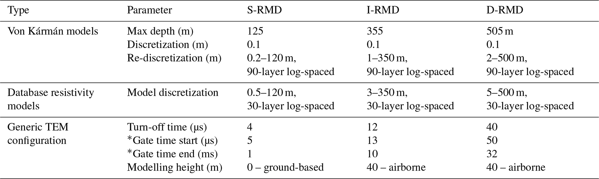
* Gate start/end times have zero-time reference at the beginning of turn-off time.
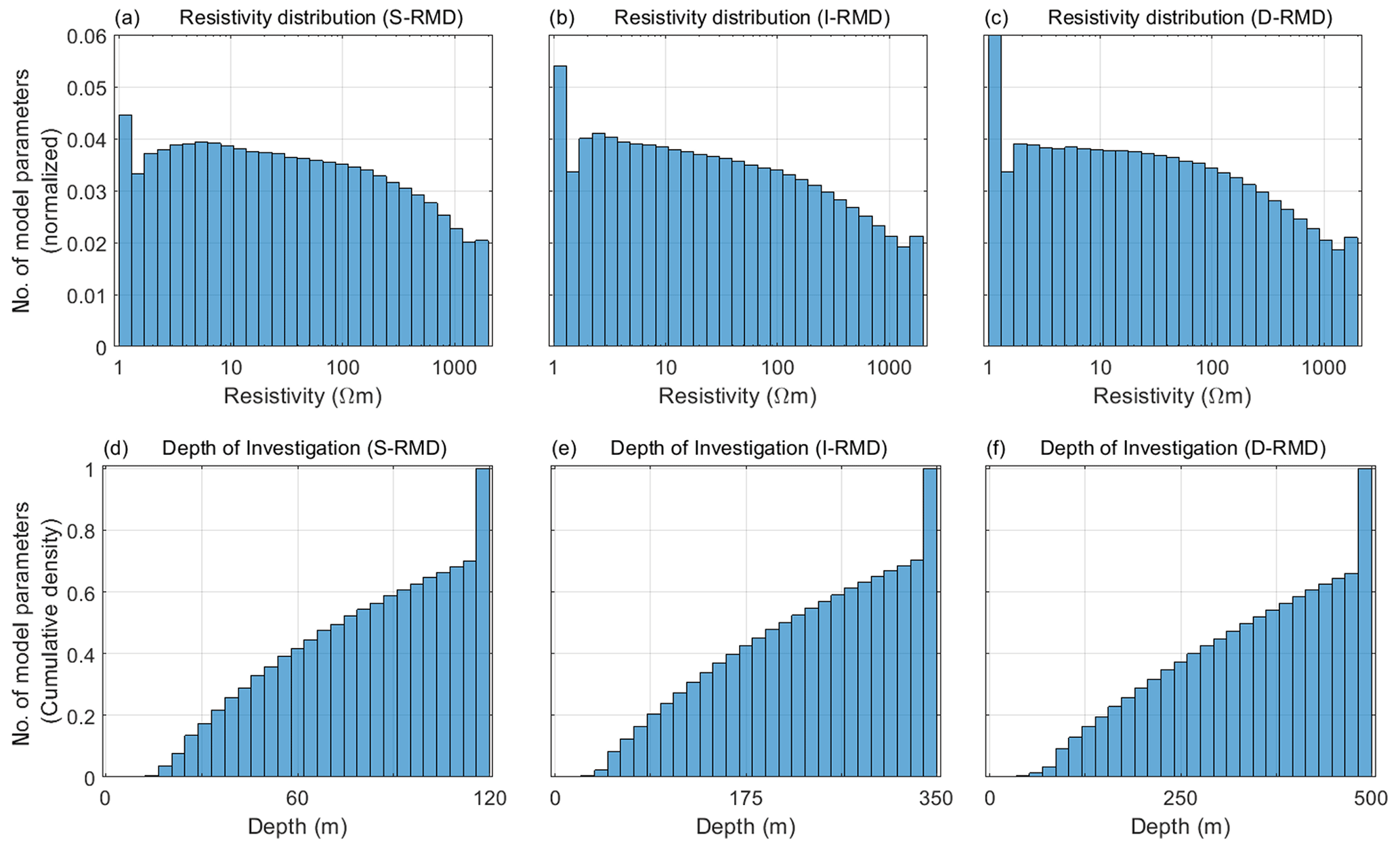
Figure 2Statistical insights into the DL-RMD. (a–c) Resistivity distributions of the S-RMD, I-RMD, and D-RMD, respectively. (d–f) Distributions of depth of investigation of models in the S-RMD, I-RMD, and D-RMD, plotted as a cumulative sum.
The model discretization details for the three DL-RMDs for the initial von Kármán models and for the final resistivity models entering the RMD are summarized in Table 3. Table 3 also holds the key specifications of the three generic TEM systems. The settings for the generation of the von Kármán models are specified in Table 2 and are common for the three DL-RMDs. Each of the three DL-RMDs holds ∼ 1 million models spanning the resistivity interval 1–2000 Ωm, where of the models originate from the initially generated von Kármán models and where of the models come from the stitched, layered von Kármán models.
Some insights into the three DL-RMDs are given in Fig. 2, where Fig. 2a–c show the layer resistivity distribution of the three DL-RMDs. The resistivity distributions of the von Kármán models were generated uniformly, but the forward and inversion process makes the resistivity distribution slightly skewed towards the lower-resistivity end, due to the lower sensitivity/resolution in the high-resistivity end for the EM method (Christiansen et al., 2006; Jørgensen et al., 2005). The larger start and end bins compared to the neighbouring bins in Fig. 2a–c are due to the 1 and 2000 Ωm resistivity truncation. The estimated depths of investigation for the three DL-RMDs are shown in Fig. 2d–f. We observe that approximately 70 % of the models have depths of investigation that are less than the depth to last layer boundary of the given DL-RMD. Notably, a thick conductive layer near the surface will significantly limit the depth of investigation for a given TEM configuration. The uneven and in some cases limited depth of investigation does not pose a problem for a deep learning algorithm, as the EM method will compromise a similar depth of investigation limitation for the given resistivity model (see the Discussion section for more details).
EM methods can benefit from the presented DL-RMD in many ways. For example, the DL-RMD can be used to surrogate the computationally expensive numerical forward modelling by using a computationally efficient DL method, which would speed up the whole inversion process. It can also be used to develop a DL algorithm to replace the calculation of the partial derivatives in deterministic inversion methods, where the subsurface resistivity model is updated iteratively by using the partial derivatives of the model parameters. Detecting anomalies in the EM data by using a DL approach using the DL-RMD can significantly speed up the EM data processing and limit the involvement of human-centric manual workflows. Additionally, EM data de-noising also becomes plausible.
As an example in this paper, we use the DL-RMD to surrogate the forward modelling problem for a ground-based TEM system using a fast DL method, since a significant number of forward calculations are required during the inversion process, when either deterministic or stochastic inversion methods are used. By replacing the computationally expensive numerical forward modelling approach, the whole inversion process may be accelerated without further modification to a standard inversion workflow (Asif et al., 2021b). However, it is crucial that the performance of the DL method balances the numerical precision and increased speed of computation. If the prediction accuracy is not sufficiently high, the application in an inversion framework may result in spurious subsurface features and erroneous geological interpretations of the geophysical EM mapping results.
4.1 Deep learning (DL) setup
We design the surrogate model for the tTEM system (Auken et al., 2018). The tTEM system is a ground-based towed TEM system with a maximum depth of investigation of 120 m based on the data time interval from ∼ 5 µs to ∼ 1 ms, which matches the specification of S-RMD; therefore, we use it to train our DL method.
The input to the DL algorithm becomes the 30-layer resistivity model m in S-RMD, where the layer thickness of each resistivity layer is fixed. The target outputs are the numerical TEM forward responses, i.e. , for the corresponding inputs. A standard EM modelling code (Auken et al., 2015) is used to generate the TEM forward responses for the resistivity models m with fixed layer thicknesses. We generate the responses from ∼ 1 ns to ∼ 10 ms by exponentially increasing gate widths sampled at 14 gates per decade.
Prior to the training of a DL method, inputs and the corresponding target outputs are normalized. Each resistivity model m is normalized, where the logarithmic variations in the model parameters can take both positive and negative values.
where mmin and mmax are the minimum and maximum resistivity values in the training dataset of S-RMD, and μ is the mean.
The target outputs, i.e. , are normalized by
where μ is the mean, and σ is the standard deviation of each data point in the training dataset.
We use a simple DL method where a fully connected feed-forward neural network is utilized with two hidden layers, each having 384 neurons. The hyperbolic tangent function is used as an activation function between the hidden layers, and the full-batch scaled conjugate algorithm is used for backpropagation. The loss function for training is the sum of squared errors with a regularization term consisting of the mean of sum of squares of the network weights and biases. The network configuration used here is based on our previous results (Asif et al., 2021b, 2022b). We also apply an early-stopping criterion to ensure that the training stops when the validation loss starts to increase. The validation set for the early-stopping criterion comprises of 70 000 models from S-RMD, which are excluded from the training set. Once the network is trained, it can be used for evaluation purposes. The evaluation metric for our baselines is the percentage relative error, RLP, defined in Eq. (4), which effectively deals with the large dynamic range and patterns of TEM data.
where is the output of the DL method, and is the numerically computed forward response.
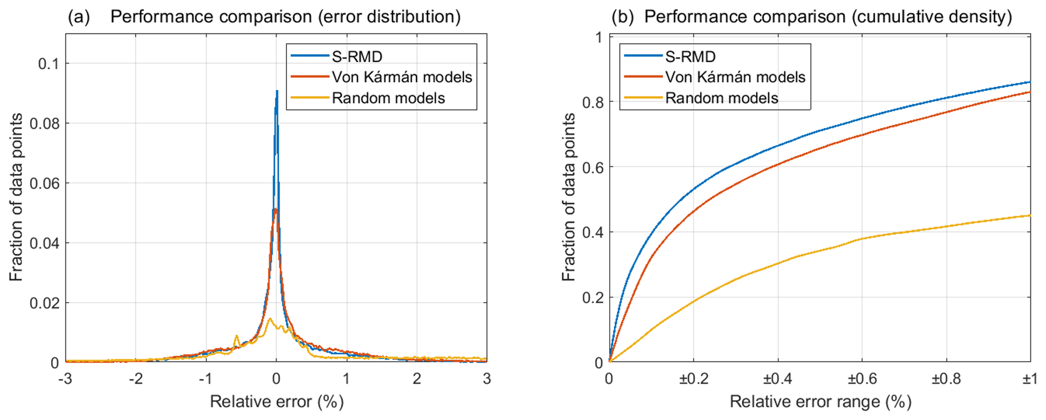
Figure 3Performance of the networks trained on S-RMD, von Kármán models, and random resistivity models. (a) RLP distribution. (b) Cumulative distribution of RLP.
4.2 Surrogate forward-modelling results
To test the performance of our DL method trained on S-RMD, we use 697 resistivity models inverted from field data from a survey conducted in Søften, a region in Denmark. The data processing and inversion step of the field data follows the method developed by Auken et al. (2018), which covers averaging, anomaly detection, manual inspection, etc. on the data. The minimum and maximum resistivity values in the test dataset are 3.9 and 127.1 Ωm, respectively. The forward responses of the field-inverted resistivity models are calculated numerically to compare them with the output of our DL method. Since the output of our DL algorithm is the normalized forward response, it is de-normalized to raw data values by manipulating Eq. (3). For a relative comparison, we train another DL network with the same configuration using the initial von Kármán resistivity models. The comparison to the initial von Kármán resistivity models also allows us to examine the effect of the forward/inversion process, as described in Sect. 2, in the generation of the DL-RMD. We also train an additional network using the random resistivity models, similarly to several DL studies (Colombo et al., 2021b; Moghadas, 2020; Moghadas et al., 2020; Noh et al., 2020; Puzyrev and Swidinsky, 2021; Qin et al., 2019; Wu et al., 2021b) as mentioned in Table 1. To have the same level of complexity, the number of layers, depth discretization, and the number of random resistivity models are kept the same as used to train the other two networks for a fair comparison, and the resistivity of each layer is chosen randomly from a log-uniform distribution to take into account the non-linearity of the forward responses with the resistivity values. As such, a resistivity change from 1 to 10 Ωm would affect the forward data more than a change from 100 to 110 Ωm (Asif et al., 2021a).
Figure 3 shows the performance comparison of the trained networks based on the evaluation metric in Eq. (3) against the forward responses of 697 resistivity models from the Søften survey. Figure 3a shows the distribution of RLP of the DL network trained on S-RMD. We also show the accuracy performance of the DL networks trained on von Kármán and the random resistivity models. It is evident that the network trained on S-RMD results in lower errors as compared to the network trained on von Kármán resistivity models. On the other hand, the network trained on random resistivity models results in a poor accuracy performance. In quantitative terms, 71 % of the data points are evaluated to be within half a percent relative error for the network trained on S-RMD. In comparison to S-RMD, the network trained on von Kármán resistivity models results in 65 % of data points within half a percent relative error. The network trained on random resistivity models performs the worst, and only 34 % of the data points are calculated to be within half a percent relative error.
We also show the cumulative distribution of RLP for the networks trained on S-RMD, von Kármán models, and random models in Fig. 3b. A maximum of 9 % improvement in accuracy is achieved for the network trained on the S-RMD as compared to the von Kármán models. In comparison to the network trained on random resistivity models, an improvement of 43 % is achieved when S-RMD is used for training. The increase in accuracy is achieved only by using an appropriate dataset for training. The prediction accuracy can be improved with different data pre-processing, network configurations, loss functions, etc. while using the same training dataset to allow for consistency in benchmarking of DL algorithms. It is also important that a balance between the prediction performance and computational efficiency is maintained. As such, the computational time for the forward pass of the proposed network configuration can serve as a baseline for time comparison.
Figure 4 shows a visual comparison of a numerical forward response against the forward response from the trained networks for one of the resistivity models from the Søften survey. It is evident from Fig. 4 that the forward response from the network trained on S-RMD is the most accurate and has a maximum relative error of 1.4 % for the data point at ∼ 72 µs (see Fig. 4a). The highest error for the forward response from the network trained on von Kármán models is observed to be 2.5 % for the data point at ∼ 160 µs as shown in Fig. 4b. The forward response from the network trained on random models results in the worst accuracy performance and results in a maximum error of 22.3 % for the data point at 100 µs (see Fig. 4c).
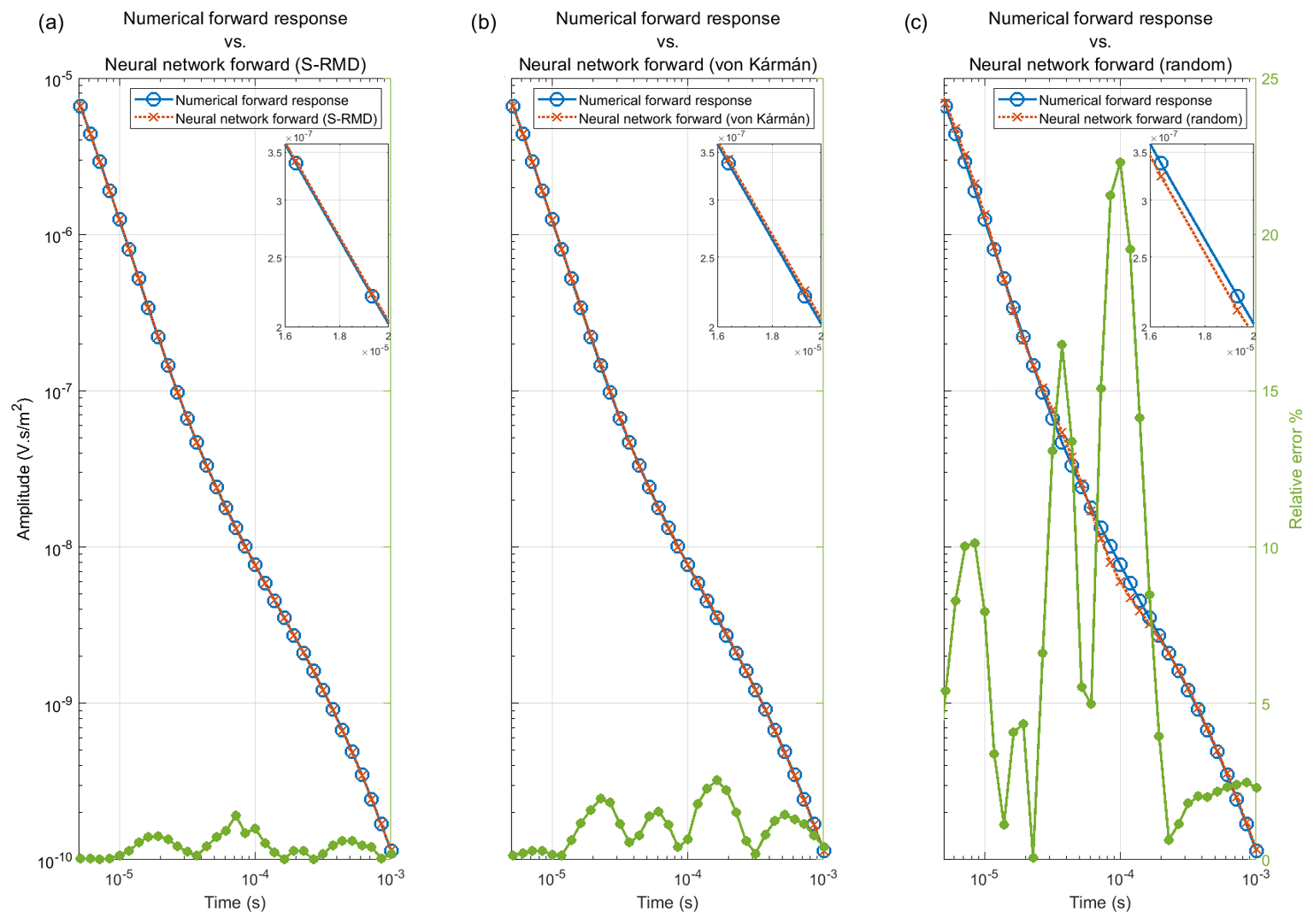
Figure 4Comparison of performance of the networks trained on S-RMD, von Kármán models, and random resistivity models with a numerical forward response from the test set. The forward responses are shown only within the time range of tTEM data, and the inset shows the forward response from 16 to 20 µs (a) Numerical forward response vs. the forward response from the network trained on S-RMD. (b) Numerical forward response vs. the forward response from the network trained on von Kármán models. (c) Numerical forward response vs. the forward response from the network trained on random resistivity models.
The network trained on random resistivity models results in a poor accuracy performance as many of the resistivity models in the training dataset are geologically unrealistic. The complex, unrealistic resistivity structures in the randomly generated training models would result in forward responses similar to the ones obtained from simpler resistivity models, which further decreases the quality of the training dataset. The von Kármán models may be considered pseudorandom resistivity models where the resistivity structure of the models has a geologically realistic nature, as it considers multiple correlation lengths with a stochastic nature resembling geological processes. Due to the geological nature of the von Kármán models, the network trained on such models results in a decent performance accuracy. However, the network trained on von Kármán models has a lower accuracy performance as compared to the network trained on S-RMD, where the resolution capability of the EM method has been taken into account, resulting in resistivity structures resolvable by the EM method.
The resolution capability and the depth of investigation for a given TEM system strongly depend on the underlying resistivity model. Therefore, stating a single depth of investigation value for a given TEM system is not appropriate. A single exploration depth, depth of investigation, or a similar value stated by the instrument manufacturers will often be an optimistic one. For TEM systems with short transmitter current turn-off, the early data points provide the near-surface resolution, while the late data points strongly control the depth of investigation for a given resistivity model. The transmitter moment and the background noise level also influence the depth of investigation, but these factors are not considered in our case, since we have assumed a uniform data uncertainty in the forward and inversion process. The three DL-RMDs span different TEM systems and resolutions. Therefore, for a particular TEM system, one should pick the DL-RMD that has a similar resolution as the underlying generic TEM system. This is best evaluated by matching the time interval of the data for the particular TEM system to the data time interval (data time start/end in Table 3) for the generic TEM system.
In Table 4, we list some examples of the compatibility of our DL-RMD with some well-known TEM systems. Despite I-RMD and D-RMD being compiled for a generic airborne system, I-RMD and D-RMD are also appropriate for ground-based TEM systems since the simulated flight altitude of 40 m does not lead to a drastic change in the vertical resolution.
Since FEM and TEM systems follow the same laws of physics, the DL-RMD is also applicable for many FEM systems, despite the generic EM system in the forward/inversion process mimicking the TEM systems. In general, the FEM systems have a shallower depth of investigation than that of the TEM systems, hence, the S-RMD is best suited for FEM systems. An alternative to the DL-RMD is to generate the resistivity model realizations by following the described methodology for the specific EM system by using the von Kármán models provided (Asif et al., 2022a). This will ensure a 100 % match between resolution, depth of investigation, etc. in the model domain compared to sensitivity in the EM data domain.
Despite the initial von Kármán models with superimposed layering, the resistivity models in the DL-RMD have a pronounced vertical smooth behaviour due to the minimum structure (smooth) regularization scheme (Viezzoli et al., 2008) used in the inversion phase. When applying another regularization scheme in the inversion phase, e.g. the minimum support norm (Vignoli et al., 2015), or when using a few-layer model discretization with no vertical regularization, one could compile a resistivity model database with different appearances. For our DL-RMD, we chose the minimum structure regularization scheme, since it is commonly used for inverting airborne and ground-based EM data. It is important to point out that a TEM data curve itself does not hold information about whether subsurface boundaries are smooth or sharp. As such, both smooth and sharp-layered models will explain the recorded data equally well in most cases. With our approach of compiling resistivity models, we have tried to avoid the inclusion of models with different smooth/sharp behaviours that result in identical or close to identical forward data responses (equivalent models).
The DL-RMD is generated in the resistivity range of 1–2000 Ωm, which covers most of the geological settings, taking into account the EM mapping capability in the high-resistivity range. The resistivity limit of 2000 Ωm was chosen since EM methods have no or very low sensitivity in the high-resistivity range, since high-resistivity materials (granite, basalt, glacier ice, etc.) produce an EM signal below the detection level. Despite the 2000 Ωm limit, the resistivity distribution of the models in the DL-RMD is slightly skewed towards lower resistivities due to the limited sensitivity of the EM method to high-resistivity values. A slight bias towards lower-resistivity values may affect the performance of a DL method for highly resistive models. However, even if an actual subsurface model is represented by a highly resistive model, it is expected that any TEM method would have difficulty in resolving such a model. The RMD also has a limitation in the low-resistivity end, e.g. in settings with seawater and saltwater intrusion, which may result in subsurface materials with resistivity values below 1 Ωm.
Since the 1-D models of the DL-RMD hold resistivity variations in one dimension (vertical) only, they cannot be used for calculating 2-D or 3-D EM responses. Examples of geological settings where a 1-D approach would be inappropriate include steep-dipping geological structures, thin sheet mineralization, mapping close to or on the shoreline, or areas with strong topographical variations. However, one could apply the same methodology to compile a 2-D or 3-D resistivity database. In this case, one would generate the initial von Kármán models as a 2-D section or 3-D volumes and use a 2-D or 3-D forward and inversion process, which of course would be much more computationally expensive compared to the 1-D case. However, the DL-RMD provided in this study opens up the possibility of exploring more deep learning frameworks, which have reliability and consistency in performance comparisons for 1-D models.
The DL-RMD is freely available at https://doi.org/10.5281/zenodo.7260886 (Asif et al., 2022a), and a ready-to-run demo code in Python Jupyter Notebook that uses the network trained on S-RMD and reproduces the results of this paper is available at https://github.com/rizwanasif/DL-RMD (last access: 17 March 2023) (DOI: https://doi.org/10.5281/zenodo.7740243, Asif, 2023).
The EM modelling code “AarhusInv” used to generate EM forward responses in this study is freely available to researchers for non-commercial activities. The details are available at https://hgg.au.dk/software/aarhusinv (Auken et al., 2015).
We have presented a methodology for compiling a geophysically constrained subsurface resistivity model database for applications related to electromagnetic data. We generated three 1-D resistivity databases, discretized to depths of 120, 350, and 500 m in the resistivity range of 1–2000 Ωm, hence covering various ground-based and airborne frequency-domain and time-domain electromagnetic systems and most of the geological settings. The upper resistivity limit of the model database is satisfactory as the electromagnetic methods have limitations for high resistivity; however, the model database has limitations in the low resistivity limit for subsurface materials below 1 Ωm that may occur in some cases. Additionally, the database holds 1-D models and therefore inherits the limitations of 1-D electromagnetic modelling.
An example is included using the proposed resistivity model database and deep learning for surrogating TEM forward modelling, showing that high accuracy can be obtained with our resistivity model database. Furthermore, the example shows that the forward/inversion steps in the generation of the database lead to a significantly increased performance in the forward modelling.
Despite some limitations, the generated resistivity model database is a well-organized database, which empowers the geoscience community to have consistency and credibility in the development of deep learning methods for many tasks including surrogating forward modelling, inverse modelling, data de-noising, automatic data processing, etc. Therefore, we urge the geophysical community to utilize the presented database to develop and investigate different network configurations, data pre-processing strategies, loss functions, etc. while using the presented model database to allow for consistency in benchmarking deep learning algorithms. The resistivity model database has already proven valuable in significantly improving the accuracy of neural networks for the forward modelling of electromagnetic data.
Conceptualization: MRA and TB. Data curation, software, and visualization: MRA. Formal analysis, methodology, and investigation: MRA, NF, TB, and AVC. Funding acquisition, project administration, resources, and supervision: JJL and AVC. Validation: NF and MRA. Writing; original draft preparation, review and editing: MRA, NF, TB, JJL, and AVC.
The contact author has declared that none of the authors has any competing interests.
Publisher’s note: Copernicus Publications remains neutral with regard to jurisdictional claims in published maps and institutional affiliations.
This article is part of the special issue “Benchmark datasets and machine learning algorithms for Earth system science data (ESSD/GMD inter-journal SI)”. It is not associated with a conference.
The authors would like to thank the handling chief editor Kirsten Elger, topical editor Martin Schultz, and the two anonymous reviewers for their comments and feedback on this paper.
This work has been supported by the Innovation Fund Denmark (IFD) under the projects “MapField” (grant no. 8055-00025B) and “SuperTEM” (grant no. 0177-00085B).
This paper was edited by Martin Schultz and reviewed by two anonymous referees.
Asif, M. R.: rizwanasif/DL-RMD: DL-RMD (DL-RMD), Zenodo [code], https://doi.org/10.5281/zenodo.7740243, 2023.
Asif, M. R., Qi, C., Wang, T., Fareed, M. S., and Khan, S.: License plate detection for multi-national vehicles–a generalized approach, Multimed. Tools Appl., 78, 35585–35606, 2019.
Asif, M. R., Bording, T. S., Barfod, A. S., Grombacher, D. J., Maurya, P. K., Christiansen, A. V., Auken, E., and Larsen, J. J.: Effect of data pre-processing on the performance of neural networks for 1-D transient electromagnetic forward modelling, IEEE Access, 9, 34635–34646, 2021a.
Asif, M. R., Bording, T. S., Maurya, P. K., Zhang, B., Fiandaca, G., Grombacher, D. J., Christiansen, A. V., Auken, E., and Larsen, J. J.: A Neural Network-Based Hybrid Framework for Least-Squares Inversion of Transient Electromagnetic Data, IEEE T. Geosci. Remote, 60, 4503610, https://doi.org/10.1109/TGRS.2021.3076121, 2021b.
Asif, M. R., Foged, N., Bording, T., Larsen, J. J., and Christiansen, A. V.: DL-RMD: A geophysically constrained electromagnetic resistivity model database for deep learning applications, Zenodo [data set], https://doi.org/10.5281/zenodo.7260886, 2022a.
Asif, M. R., Foged, N., Maurya, P. K., Grombacher, D. J., Christiansen, A. V., Auken, E., and Larsen, J. J.: Integrating neural networks in least-squares inversion of airborne time-domain electromagnetic data, Geophysics, 87, E177–E187, https://doi.org/10.1190/geo2021-0335.1, 2022b.
Auken, E., Christiansen, A. V., Kirkegaard, C., Fiandaca, G., Schamper, C., Behroozmand, A. A., Binley, A., Nielsen, E., Effersø, F., and Christensen, N. B.: An overview of a highly versatile forward and stable inverse algorithm for airborne, ground-based and borehole electromagnetic and electric data, Explor. Geophys., 46, 223–235, https://doi.org/10.1071/EG13097, 2015 (data available at: https://hgg.au.dk/software/aarhusinv, last access: 16 March 2023).
Auken, E., Foged, N., Larsen, J. J., Lassen, K. V. T., Maurya, P. K., Dath, S. M., and Eiskjær, T. T.: tTEM – A towed transient electromagnetic system for detailed 3D imaging of the top 70 m of the subsurface, Geophysics, 84, E13–E22, 2018.
Baan, M. V. D. and Jutten, C.: Neural networks in geophysical applications, Geophysics, 65, 1032–1047, 2000.
Bai, P., Vignoli, G., Viezzoli, A., Nevalainen, J., and Vacca, G.: (Quasi-)Real-Time Inversion of Airborne Time-Domain Electromagnetic Data via Artificial Neural Network, Remote Sensing, 12, 3440, https://doi.org/10.3390/rs12203440, 2020.
Balch, S., Boyko, W., and Paterson, N.: The AeroTEM airborne electromagnetic system, The Leading Edge, 22, 562–566, 2003.
Bang, M., Oh, S., Noh, K., Seol, S. J., and Byun, J.: Imaging subsurface orebodies with airborne electromagnetic data using a recurrent neural network, Geophysics, 86, E407–E419, https://doi.org/10.1190/geo2020-0871.1, 2021.
Bergen, K. J., Johnson, P. A., Maarten, V., and Beroza, G. C.: Machine learning for data-driven discovery in solid Earth geoscience, Science, 363, eaau0323, https://doi.org/10.1126/science.aau0323, 2019.
Birken, R. A. and Poulton, M. M.: Neural Network Interpretation of High Frequency Electromagnetic Ellipticity Data Part II: Analyzing 3D Responses, Journal of Environmental Engineering Geophysics, 4, 149–165, 1999.
Birken, R. A., Poulton, M. M., and Lee, K. H.: Neural Network Interpretation of High Frequency Electromagnetic Ellipticity Data Part I: Understanding the Half-Space and Layered Earth Response, Journal of Environmental Engineering Geophysics, 4, 93–103, 1999.
Bording, T. S., Asif, M. R., Barfod, A. S., Larsen, J. J., Zhang, B., Grombacher, D. J., Christiansen, A. V., Engebretsen, K. W., Pedersen, J. B., Maurya, P. K., and Auken, E.: Machine learning based fast forward modelling of ground-based time-domain electromagnetic data, J. Appl. Geophys., 187, 104290, https://doi.org/10.1016/j.jappgeo.2021.104290, 2021.
Christiansen, A. V. and Auken, E.: Layered 2-D inversion of profile data, evaluated using stochastic models, ASEG Extended Abstracts, 1–8, https://doi.org/10.1071/ASEG2003_3DEMab005, 2003.
Christiansen, A. V. and Auken, E.: A global measure for depth of investigation, Geophysics, 77, WB171–WB177, 2012.
Christiansen, A. V., Auken, E., and Sørensen, K.: The transient electromagnetic method, in: Groundwater geophysics, edited by: Kirsch, R., Springer, ISBN 978-3-540-29383-5, https://doi.org/10.1007/3-540-29387-6_6, 2006.
Colombo, D., Li, W., Rovetta, D., Sandoval-Curiel, E., and Turkoglu, E.: Physics-driven deep learning joint inversion, in: SEG Technical Program Expanded Abstracts 2020, Society of Exploration Geophysicists, 1775–1779, https://doi.org/10.1190/segam2020-3424997.1, 2020a.
Colombo, D., Li, W., Sandoval-Curiel, E., and McNeice, G. W.: Electromagnetic reservoir monitoring with machine-learning inversion and fluid flow simulators, in: Fifth International Conference on Engineering Geophysics (ICEG), Al Ain, UAE, 21–24 October 2019, 167–170, https://doi.org/10.1190/iceg2019-043.1, 2020b.
Colombo, D., Turkoglu, E., Li, W., and Rovetta, D.: Coupled physics-deep learning inversion, Comput. Geosci., 157, 104917, https://doi.org/10.1016/j.cageo.2021.104917, 2021a.
Colombo, D., Turkoglu, E., Li, W., Sandoval-Curiel, E., and Rovetta, D.: Physics-driven deep learning inversion with application to transient electromagnetics, Geophysics, 86, E209–E224, https://doi.org/10.1190/geo2020-0760.1, 2021b.
Conway, D., Alexander, B., King, M., Heinson, G., and Kee, Y.: Inverting magnetotelluric responses in a three-dimensional earth using fast forward approximations based on artificial neural networks, Comput. Geosci., 127, 44–52, 2019.
Dong, C., Loy, C. C., and Tang, X.: Accelerating the super-resolution convolutional neural network, in: European conference on computer vision, Amsterdam, the Netherlands, 11–14 October 2016, 391–407, https://doi.org/10.1007/978-3-319-46475-6_25, 2016.
Dramsch, J. S.: 70 years of machine learning in geoscience in review, Adv. Geophys., 61, 1–55, https://doi.org/10.1016/bs.agph.2020.08.002, 2020.
Feng, X.-T. and Seto, M.: Neural network dynamic modelling of rock microfracturing sequences under triaxial compressive stress conditions, Tectonophysics, 292, 293–309, 1998.
Guo, R., Li, M., Fang, G., Yang, F., Xu, S., and Abubakar, A.: Application of supervised descent method to transient electromagnetic data inversion, Geophysics, 84, E225–E237, 2019.
Hopfield, J. J.: Neural networks and physical systems with emergent collective computational abilities, P. Natl. Acad. Sci. USA, 79, 2554–2558, 1982.
Jørgensen, F., Sandersen, P. B., Auken, E., Lykke-Andersen, H., and Sørensen, K.: Contributions to the geological mapping of Mors, Denmark – a study based on a large-scale TEM survey, B. Geol. Soc. Denmark, 52, 53–75, 2005.
Karshakov, E. V., Podmogov, Y. G., Kertsman, V. M., and Moilanen, J.: Combined Frequency Domain and Time Domain Airborne Data for Environmental and Engineering Challenges, J. Environ. Eng. Geoph., 22, 1–11, https://doi.org/10.2113/JEEG22.1.1, 2017.
Khatibi, S. and Aghajanpour, A.: Machine Learning: A Useful Tool in Geomechanical Studies, a Case Study from an Offshore Gas Field, Energies, 13, 3528, https://doi.org/10.3390/en13143528, 2020.
Kirsch, R.: Groundwater geophysics: a tool for hydrogeology, Springer, ISBN 978-3-540-29383-5, https://doi.org/10.1007/3-540-29387-6, 2006.
Krizhevsky, A., Sutskever, I., and Hinton, G. E.: ImageNet classification with deep convolutional neural networks, Adv. Neur. Inf. Proc. Sys., 25, 1097–1105, https://proceedings.neurips.cc/paper/2012/file/c399862d3b9d6b76c8436e924a68c45b-Paper.pdf (last access: 16 March 2023), 2012.
Krizhevsky, A., Sutskever, I., and Hinton, G. E.: Imagenet classification with deep convolutional neural networks, Communications of the ACM, 60, 84–90, 2017.
Kwan, K., Reford, S., Abdoul-Wahab, D. M., Pitcher, D. H., Bournas, N., Prikhodko, A., Plastow, G., and Legault, J. M.: Supervised neural network targeting and classification analysis of airborne EM, magnetic and gamma-ray spectrometry data for mineral exploration, ASEG Extended Abstracts, 2015, 1–5, https://doi.org/10.1071/ASEG2015ab306, 2015.
Leggatt, P. B., Klinkert, P. S., and Hage, T. B.: The Spectrem airborne electromagnetic system – Further developments, Geophysics, 65, 1976–1982, 2000.
Li, J., Liu, Y., Yin, C., Ren, X., and Su, Y.: Fast imaging of time-domain airborne EM data using deep learning technology, Geophysics, 85, E163–E170, https://doi.org/10.1190/geo2019-0015.1, 2020.
Lin, F., Chen, K., Wang, X., Cao, H., Chen, D., and Chen, F.: Denoising stacked autoencoders for transient electromagnetic signal denoising, Nonlin. Processes Geophys., 26, 13–23, https://doi.org/10.5194/npg-26-13-2019, 2019.
Liu, W., Lü, Q., Yang, L., Lin, P., and Wang, Z.: Application of Sample-Compressed Neural Network and Adaptive-Clustering Algorithm for Magnetotelluric Inverse Modeling, IEEE Geoscience Remote Sensing Letters, 18, 1540–1544, https://doi.org/10.1109/LGRS.2020.3005796, 2020.
Maurer, H., Holliger, K., and Boerner, D. E.: Stochastic regularization: Smoothness or similarity?, Geophys. Res. Lett., 25, 2889–2892, 1998.
Moghadas, D.: One-dimensional deep learning inversion of electromagnetic induction data using convolutional neural network, Geophys. J. Int., 222, 247–259, 2020.
Moghadas, D., Behroozmand, A. A., and Christiansen, A. V.: Soil electrical conductivity imaging using a neural network-based forward solver: Applied to large-scale Bayesian electromagnetic inversion, J. Appl. Geophys., 176, 104012, https://doi.org/10.1016/j.jappgeo.2020.104012, 2020.
Møller, I., Jacobsen, B. H., and Christensen, N. B.: Rapid inversion of 2-D geoelectrical data by multichannel deconvolution, Geophysics, 66, 800–808, 2001.
Noh, K., Yoon, D., and Byun, J.: Imaging subsurface resistivity structure from airborne electromagnetic induction data using deep neural network, Explor. Geophys., 51, 214–220, 2020.
Pang, X., Zhou, Y., Wang, P., Lin, W., and Chang, V.: An innovative neural network approach for stock market prediction, J. Supercomput., 76, 2098–2118, 2020.
Poulton, M. M., Sternberg, B. K., and Glass, C. E.: Location of subsurface targets in geophysical data using neural networks, Geophysics, 57, 1534–1544, 1992.
Puzyrev, V.: Deep learning electromagnetic inversion with convolutional neural networks, Geophys. J. Int., 218, 817–832, 2019.
Puzyrev, V. and Swidinsky, A.: Inversion of 1D frequency-and time-domain electromagnetic data with convolutional neural networks, Comput. Geosci., 149, 104681, https://doi.org/10.1016/j.cageo.2020.104681, 2021.
Qin, S., Wang, Y., Tai, H.-M., Wang, H., Liao, X., and Fu, Z.: TEM apparent resistivity imaging for grounding grid detection using artificial neural network, IET Generation, Transmission, Distribution, 13, 3932–3940, https://doi.org/10.1049/iet-gtd.2018.6450, 2019.
Redmon, J., Divvala, S., Girshick, R., and Farhadi, A.: You only look once: Unified, real-time object detection, in: Proceedings of the IEEE conference on computer vision and pattern recognition, Las Vegas, NV, USA, 27–30 June 2016, 779–788, https://doi.org/10.1109/CVPR.2016.91, 2016.
Reichstein, M., Camps-Valls, G., Stevens, B., Jung, M., Denzler, J., and Carvalhais, N.: Deep learning and process understanding for data-driven Earth system science, Nature, 566, 195–204, 2019.
Ren, S., He, K., Girshick, R., and Sun, J.: Faster r-cnn: Towards real-time object detection with region proposal networks, Adv. Neur. In., 1, 91–99, 2015.
Röth, G. and Tarantola, A.: Neural networks and inversion of seismic data, J. Geophys. Res.-Sol. Ea., 99, 6753–6768, 1994.
Smith, R., Fountain, D., and Allard, M.: The MEGATEM fixed-wing transient EM system applied to mineral exploration: a discovery case history, First Break, 21, https://doi.org/10.3997/1365-2397.21.7.25570, 2003.
Smith, R. S.: Airborne electromagnetic methods: Applications to minerals, water and hydrocarbon exploration, Canadian Society of Explortation Geophysics, 35, 7–10, https://csegrecorder.com/articles/view/airborne-electromagnetic-methods-app-to-minerals-water-hydrocarbon-expl (last access: 16 March 2023), 2010.
Sørensen, K. I. and Auken, E.: SkyTEM-A new high-resolution helicopter transient electromagnetic system, Explor. Geophys., 35, 191–199, 2004.
Tacher, L., Pomian-Srzednicki, I., and Parriaux, A.: Geological uncertainties associated with 3-D subsurface models, Comput. Geosci., 32, 212–221, 2006.
Viezzoli, A., Christiansen, A. V., Auken, E., and Sørensen, K.: Quasi-3D modeling of airborne TEM data by spatially constrained inversion, Geophysics, 73, F105–F113, 2008.
Vignoli, G., Fiandaca, G., Christiansen, A. V., Kirkegaard, C., and Auken, E.: Sharp spatially constrained inversion with applications to transient electromagnetic data, Geophys. Prospect., 63, 243–255, 2015.
Wang, W., Zhang, M., Chen, G., Jagadish, H., Ooi, B. C., and Tan, K.-L.: Database meets deep learning: Challenges and opportunities, ACM SIGMOD Record, 45, 17–22, 2016.
Wu, S., Huang, Q., and Zhao, L.: Convolutional neural network inversion of airborne transient electromagnetic data, Geophys. Prospect., 69, 1761–1772, 2021a.
Wu, S., Huang, Q., and Zhao, L.: De-noising of transient electromagnetic data based on the long short-term memory-autoencoder, Geophys. J. Int., 224, 669–681, 2021b.
Xue, G., Li, H., He, Y., Xue, J., and Wu, X.: Development of the Inversion Method for Transient Electromagnetic Data, IEEE Access, 8, 146172–146181, https://doi.org/10.1109/ACCESS.2020.3013626, 2020.
Zhang, R., Liu, Y., and Sun, H.: Physics-guided convolutional neural network (PhyCNN) for data-driven seismic response modeling, Eng. Struct., 215, 110704, https://doi.org/10.1016/j.engstruct.2020.110704, 2020.
Zhang, Y. and Paulson, K.: Regularized hopfield neural networks and its application to one-dimensional inverse problem of magnetotelluric observations, Inverse Probl. Eng., 5, 33–53, 1997.
Zhang, Y., Pezeshki, M., Brakel, P., Zhang, S., Bengio, C. L. Y., and Courville, A.: Towards end-to-end speech recognition with deep convolutional neural networks, arXiv [preprint], https://doi.org/10.48550/arXiv.1701.02720, 10 January 2017.
Zhang, Z., Qi, C., and Asif, M. R.: Investigation on Projection Space Pairs in Neighbor Embedding Algorithms, 2018 14th IEEE International Conference on Signal Processing (ICSP), Beijing, China, 12–16 August 2018, 125–128, https://doi.org/10.1109/ICSP.2018.8652441, 2018.
Zhdanov, M. S.: Inverse theory and applications in geophysics, 2nd edn., Elsevier, ISBN 978-0-444-62674-5, https://doi.org/10.1016/C2012-0-03334-0, 2015.
Zhu, K.-G., Ma, M.-Y., Che, H.-W., Yang, E.-W., Ji, Y.-J., Yu, S.-B., and Lin, J.: PC-based artificial neural network inversion for airborne time-domain electromagnetic data, J. Appl. Geophys., 9, 1–8, https://doi.org/10.1007/s11770-012-0307-7, 2012.
- Abstract
- Introduction
- Methodology
- Deep learning resistivity model database (DL-RMD)
- Example of an EM application using the DL-RMD
- Discussion
- Code and data availability
- Conclusion
- Author contributions
- Competing interests
- Disclaimer
- Special issue statement
- Acknowledgements
- Financial support
- Review statement
- References