the Creative Commons Attribution 4.0 License.
the Creative Commons Attribution 4.0 License.
 | 21 Feb 2022
Reconstruction of a daily gridded snow water equivalent product for the land region above 45° N based on a ridge regression machine learning approach
Donghang Shao
Hongyi Li
Jian Wang
Xiaohua Hao
Wenzheng Ji
The snow water equivalent (SWE) is an important parameter of surface hydrological and climate systems, and it has a profound impact on Arctic amplification and climate change. However, there are great differences among existing SWE products. In the land region above 45∘ N, the existing SWE products are associated with a limited time span and limited spatial coverage, and the spatial resolution is coarse, which greatly limits the application of SWE data in cryosphere change and climate change studies. In this study, utilizing the ridge regression model (RRM) of a machine learning algorithm, we integrated various existing SWE products to generate a spatiotemporally seamless and high-precision RRM SWE product. The results show that it is feasible to utilize a ridge regression model based on a machine learning algorithm to prepare SWE products on a global scale. We evaluated the accuracy of the RRM SWE product using hemispheric-scale snow course (HSSC) observational data and Russian snow survey data. The mean absolute error (MAE), RMSE, R, and R2 between the RRM SWE products and observed SWEs are 0.21, 25.37 mm, 0.89, and 0.79, respectively. The accuracy of the RRM SWE dataset is improved by 28 %, 22 %, 37 %, 11 %, and 11 % compared with the original AMSR-E/AMSR2 (SWE), ERA-Interim SWE, Global Land Data Assimilation System (GLDAS) SWE, GlobSnow SWE, and ERA5-Land SWE datasets, respectively, and it has a higher spatial resolution. The RRM SWE product production method does not rely heavily on an independent SWE product; it takes full advantage of each SWE dataset, and it takes into consideration the altitude factor. The MAE ranges from 0.16 for areas within <100 m elevation to 0.29 within the 800–900 m elevation range. The MAE is best in the Russian region and worst in the Canadian region. The RMSE ranges from 4.71 mm for areas within <100 m elevation to 31.14 mm within the >1000 m elevation range. The RMSE is best in the Finland region and worst in the Canadian region. This method has good stability, is extremely suitable for the production of snow datasets with large spatial scales, and can be easily extended to the preparation of other snow datasets. The RRM SWE product is expected to provide more accurate SWE data for the hydrological model and climate model and provide data support for cryosphere change and climate change studies. The RRM SWE product is available from “A Big Earth Data Platform for Three Poles” (https://doi.org/10.11888/Snow.tpdc.271556) (Li et al., 2021).
- Article
(13359 KB) - Full-text XML
- BibTeX
- EndNote


The IPCC (Intergovernmental Panel on Climate Change) AR6 (Sixth Assessment Report) notes that the Northern Hemisphere spring snow cover has greatly decreased since 1950, and the feedback effect of the climate system caused by this reduction is extremely large (Masson-Delmotte et al., 2021). In most land areas of the Northern Hemisphere, annual runoff is dominated by snowmelt, and accurately estimating the impacts of such a large amount of snowmelt runoff on ecosystems and human activities is of great significance (Barnett et al., 2005; Bintanja and Andry, 2017; Henderson et al., 2018). Whether through hydrometeorological simulation or global change research, the estimation of the energy budget and mass of snow is very difficult, so a set of highly accurate, long time series snow cover datasets is urgently needed to drive hydrometeorological simulations and land surface process models. Among them, snow water equivalent (SWE) data play an irreplaceable role as an important parameter of the land surface hydrological model and climate model.
At present, there are many forms of SWE data in the world. According to type, these data can be divided into site observational SWE, remote sensing SWE, reanalysis SWE, data assimilation SWE, and model simulation SWE. The remote sensing SWEs are mainly AMSR-E (Kelly, 2009) and AMSR2 (Imaoka et al., 2010; Tedesco and Jeyaratnam, 2019). The reanalysis SWE was mainly based on the ERA-Interim (Dee et al., 2011), MERRA2 (Gelaro et al., 2017), MERRA land (Reichle et al., 2011), and ERA5-Land (Muñoz Sabater, 2019; Balsamo et al., 2015) datasets. The data assimilation SWE mainly includes GlobSnow (Luojus et al., 2021) and the Global Land Data Assimilation System (GLDAS) (Rodell et al., 2004). The site observational SWE mainly includes the GHCN dataset (Menne et al., 2016) and HSSC data (Pulliainen et al., 2020). However, the time ranges of AMSR-E and AMSR-E2 SWE are only from 2003 to the present, which is lacking in terms of time series. Similarly, the GlobSnow SWE dataset is also seriously lacking in time series. Although the reanalysis SWE data have good spatial and temporal continuity and high data integrity, their accuracy is poor, and the mean absolute error (MAE) is 0.65 (Snauffer et al., 2016). The SWE data from stations and meteorological observations cannot meet the needs of hydrometeorological and climate change research. This is mainly because SWE from stations is discontinuous in time series and severely missing. Furthermore, hydrometeorological studies often require spatiotemporally continuous grid data to be derived (Pan et al., 2003). There are great differences among remote sensing SWE, reanalysis SWE data, data assimilation SWE, and observational SWE. For remote sensing SWE, the spatiotemporal characteristics of different passive microwave SWE data differ significantly due to differences in sensors or retrieval algorithms (Mudryk et al., 2015). Data assimilation SWE and reanalysis SWE data also tend to exhibit different spatiotemporal characteristics due to differences in model design, driving data, and assimilation methods (Vuyovich et al., 2014). In summary, although there are a variety of SWE data in the world, the data quality is uncertain.
Previous studies have shown that all kinds of SWE data in the Northern Hemisphere have advantages and disadvantages, and none of these data perform well in all aspects (Mortimer et al., 2020). An effective method was used in a study by Pulliainen et al. (2020), who applied a bias correction to GlobSnow and reanalysis data products based on SWE snow course measurements to obtain improved estimates on annual peak snow mass and SWE in the Northern Hemisphere. Another effective method is to fuse all kinds of SWE data in time and space, integrate the advantages of all kinds of data, and then generate a relatively complete SWE dataset. Many scholars have conducted in-depth studies on SWE data fusion. The main fusion methods can be classified into the following categories: multiproduct direct averaging (Mudryk et al., 2015), linear regression (Snauffer et al., 2016), data assimilation (Pulliainen, 2006), “multiple” collocation (Pan et al., 2015), and machine learning (Snauffer et al., 2018; Xiao et al., 2018; Wang et al., 2020). Studies have shown that even the simplest multisource data average is more accurate than a single SWE product (Snauffer et al., 2018). However, the simple multisource data average cannot highlight the advantages of high-precision data, and it is easily affected by the weight ratio of low-precision data, which reduces the accuracy of fused data (Mudryk et al., 2015). Although the linear regression method can make good use of the actual observational data to correct the original data, it is easy to overfit which causes the overall deviation (Snauffer et al., 2016). The “multiple” collocation method changes the size of the original SWE data before fusion, which easily causes data errors. The data assimilation method is sensitive to the accuracy of input data, and it is difficult to fuse multisource data (Pan et al., 2015). In recent years, machine learning methods have been widely used in data fusion (Santi et al., 2021; Ntokas et al., 2021). Machine learning methods can not only integrate the advantages of multisource data but also make full use of site observational data to train the sample data, which easily generates SWE data products with large spatial scales and long time series (Broxton et al., 2019; Bair et al., 2018).
In summary, based on the existing SWE data products, combining a machine learning algorithm to fuse multisource SWE data is an effective method to prepare SWE products with long time series and large spatial scales and retain the advantages of single SWE data products. The ridge regression model is a biased estimation method specifically designed to address the problem of multicollinear data (Duzan and Shariff, 2015; Saleh et al., 2019). It has good tolerance to “ill-conditioned” data and has a good effect in using SWE data to address the multicollinearity problem (Hoerl and Kennard, 1970b; Guilkey and Murphy, 1975). In this study, we integrated multisource SWE data products of the ridge regression model (RRM) SWE based on the ridge regression model of the machine learning algorithm. We selected ERA-Interim SWE, GLDAS SWE, GlobSnow SWE, AMSR-E/AMSR2 SWE, and ERA5-Land SWE data with relatively complete time series as the original data for the production of the RRM SWE product. The missing parts of the ERA-Interim SWE, AMSR-E/AMSR2 SWE, and GlobSnow SWE data were filled by the spatiotemporal interpolation method. The HSSC dataset (Pulliainen et al., 2020) and Russian snow survey data (Bulygina et al., 2011) were used as training sample data of “true SWE”, and the effect of altitude on the algorithm was also considered. Thus, we prepared a set of spatiotemporal seamless SWE datasets (RRM SWE) covering the land region above 45∘ N from 1979 to 2019. The spatial coverage of the RRM SWE product covers all land regions north of 45∘ N.
2.1 Research region
The research region of the RRM SWE product is located in the land region north of 45∘ N (Fig. 1). This region consists of Asia, Europe, and North America. The land region covers Russia, the United States, Canada, Denmark, Norway, Iceland, Sweden, and Finland. This region has a cold climate and a wide area of snow cover.
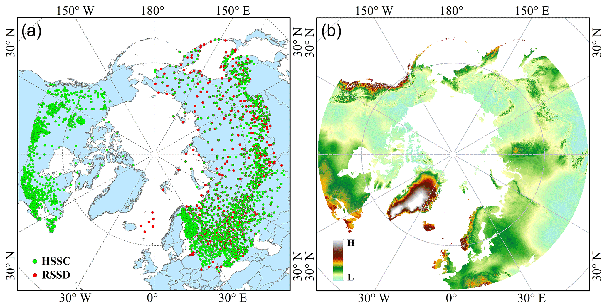
Figure 1The DEM and snow survey stations of the research region. The right panel (b) shows the DEM, and the left panel (a) shows the SWE observational stations. HSSC, hemispheric-scale snow course; RSSD, the Russian snow survey station. The spatial range of the RRM SWE product is consistent with that of the DEM.
2.2 Grid SWE data description
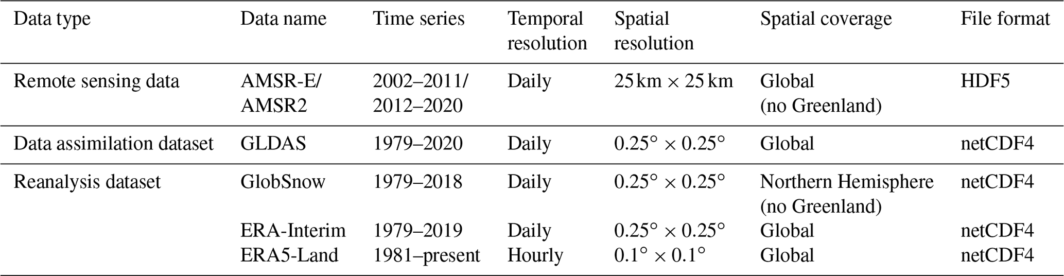
In this study, we utilized ERA-Interim SWE data (Dee et al., 2011), GLDAS SWE data (Rodell et al., 2004), GlobSnow SWE data (Luojus et al., 2021), AMSR-E/AMSR2 SWE data (Tedesco and Jeyaratnam, 2019), and ERA5-Land SWE data (Muñoz Sabater, 2019) as the original input datasets for the fusion data (Table 1).
GlobSnow is a dataset of global snow cover and SWEs for the Northern Hemisphere released by the European Space Agency (ESA) (http://www.globsnow.info/swe/,last access: 17 February 2022) (Luojus et al., 2021; Pulliainen et al., 2020). The SWE products in this dataset combine the Canadian Meteorological Center (CMC) daily snow depth analysis data (Walker et al., 2011), ground weather site observational data, and satellite microwave radiometer data. We obtained the L3A_daily_SWE product of this dataset. The temporal resolution of the L3A_daily_SWE product is daily, the spatial resolution is 0.25∘, and the data format is netCDF4.
ERA-Interim is the fourth generation reanalysis data of the European Centre for Medium-Range Weather Forecasts (ECMWF) (Dee et al., 2011). The data provide a global assimilated numerical product of various surface and top atmospheric parameters from January 1979 to the present (https://apps.ecmwf.int/datasets/data/interim-full-daily/levtype=sfc/, last access: 17 February 2022). We obtained the SWE dataset with a daily temporal resolution, a spatial resolution of 0.25∘, and netCDF4 data format. The spatial range of the data is the land region above 45∘ N.
The Advanced Microwave Scanning Radiometer-Earth Observation System (AMSR-E) is a microwave scanning radiometer on the Aqua satellite of the National Aeronautics and Space Administration (NASA) Earth Observation System (EOS) (Tedesco and Jeyaratnam, 2019). The AMSR-E provides a global daily SWE dataset from 19 June 2002 to 3 October 2011 (https://nsidc.org/data/ae_dysno, last access: 17 February 2022). AMSR2 is a microwave scanning radiometer on the GCOM-W1 satellite launched by the Japan Aerospace Exploration Agency (JAXA) in May 2012. AMSR2 provides a global SWE dataset from 2 July 2012 to the present (https://nsidc.org/data/AU_DySno/versions/1, last access: 17 February 2022). The spatial resolution of the AMSR-E SWE and AMSR2 SWE datasets is 25 km×25 km, the temporal resolution is daily, and the data formats are HDF-EOS and HDF-EOS5, respectively.
The GLDAS is a model used to describe global land information; it contains data, such as global rainfall, water evaporation, surface runoff, underground runoff, soil moisture, surface snow cover distribution, temperature, and heat flow distribution (Rodell et al., 2004). This assimilation system includes data with spatial resolutions of and and temporal resolutions of 3 h, 1 d, and 1 month. The GLDAS data are available for download from the Goddard Earth Sciences Data and Information Services Center (GES DISC). We obtain an SWE dataset with a daily temporal resolution, 0.25∘ spatial resolution, and netCDF4 data format.
ERA5-Land is a reanalysis dataset that provides the evolution of global land parameter data from 1981 onwards (Muñoz Sabater, 2019). The dataset provides eight types of snow parameter data, including snow albedo, snow cover, snow depth, snowfall, the temperature of the snow layer, snowmelt, snow density, and SWE. This dataset provides a global SWE dataset with an hourly spatial resolution, a temporal resolution of , a temporal coverage of January 1981 to the present, and data formats of GRIB (General Regularly-distributed Information in Binary form) and netCDF4.
To maintain consistency in the spatial and temporal resolutions of the fused data, we unified the ERA-Interim SWE data, GLDAS SWE data, GlobSnow SWE data, AMSR-E/AMSR2 SWE data, and ERA5-Land SWE data into a daily temporal resolution, with a spatial resolution of 0.25∘ and geographic projection of the North Pole Lambert azimuthal equal area.
2.3 Ridge regression machine learning algorithm for preparing the SWE
In this study, we utilize the ridge regression model of a machine learning algorithm to fuse ERA-Interim SWE data (Dee et al., 2011), GLDAS SWE data (Rodell et al., 2004), GlobSnow SWE data (Luojus et al., 2021), AMSR-E/AMSR2 SWE data (Tedesco and Jeyaratnam, 2019), and ERA5-Land SWE data (Muñoz Sabater, 2019) to generate a set of new RRM SWE datasets. The target reference data in this study are the HSSC dataset and Russian snow survey data. The digital elevation model (DEM) was used as an important environmental feature input to the ridge regression model and was included in the model training. The DEM is an auxiliary terrain feature variable in addition to the five SWE prediction feature variables: AMSR-E/AMSR2 SWE, ERA-Interim SWE, GLDAS SWE, GlobSnow SWE, and ERA5-Land SWE.
The ridge regression model is a biased estimate regression method for collinear data analysis (Friedman et al., 2010; Hoerl and Kennard, 1970b, a). By abandoning the unbiasedness of the ordinary least squares, this algorithm can obtain the regression method in which the regression coefficient is more practical and reliable at the cost of losing part of the information and reducing the accuracy. The ridge regression model is flexible in the choice of predictor variables and does not require the predictor and target variables to be independent of each other. It can effectively solve the multicollinearity problem of predictor and target variables, as well as reduce the impact of this problem on the training model (Duzan and Shariff, 2015; Saleh et al., 2019). Generally, reanalysis data based on SWE products cannot make the products and models independent of each other; i.e., they are prone to multicollinearity, which leads to distorted model estimation or difficulty in performing accurate estimations. In contrast, the ridge regression model can successfully solve the multicollinearity problem, i.e., the independence of training products and models. In addition, when integrating multiple SWE products, the accuracy of each SWE dataset is likely to differ. A small change in one of the SWE products involved in the training will cause a significant error in the final calculation results, while the ridge regression model has high accuracy and stability for these “ill-conditioned” SWE data. In addition, the main advantage of this model is that SWE products with long time series and large spatial scales are easy to prepare. The principle equation of the ridge regression model is defined as follows:
where is the extremum solution function of ridge regression; p is the number of gridded SWE product variables involved in training; xi are the prediction feature variables, which contain two parts: one set contains the main feature variables of the gridded SWE products, and the other part consists of the DEM auxiliary feature variables; yi is the observed SWE; λ, β, βj, and β0 are the parameters to be solved; is the sample of the training dataset; and is the penalty function term. The total number of samples N in the training dataset is 271 651. The sample sizes of the training dataset, validation dataset, and test dataset are divided according to the ratio of , where the numbers of training set, validation set and test set samples are 271 651, 77 614, and 38 807, respectively. The model is developed in Python3, and the model framework is based on the “scikit-learn” machine learning library (https://scikit-learn.org/stable/index.html, last access: 17 February 2022). The code is available upon request.
The integration process of the RRM SWE product (Fig. 2) is described as follows:
-
The original ERA-Interim SWE data, GLDAS SWE data, GlobSnow SWE data, AMSR-E/AMSR2 SWE data, ERA5-Land SWE data, DEM data, unified temporal resolution, spatial resolution, projection, spatial range, and unit are preprocessed.
-
The spatiotemporal interpolation method is used to fill in the missing data of AMSR-E/AMSR2 SWE, ERA-Interim SWE, and GlobSnow SWE in space and time. Based on this method, the missing AMSR-E/AMSR2 SWE data at low latitudes and the missing ERA-Interim SWE and GlobSnow SWE data in the time series are added.
-
The SWE data observed at stations from 1979 to 2014 are used as sample training data, and the AMSR-E/AMSR2 SWE, ERA-Interim SWE, GLDAS SWE, GlobSnow SWE, ERA5-Land SWE data, and DEM data are input into the ridge regression model of a machine learning algorithm for training. During the RRM model training process, we reconstructed the training data to try to extract training samples that are uniformly distributed spatially as much as possible. First, a scan window of 250 km×250 km (10×10 pixels) was created. Then, each gridded SWE data point participating in training is scanned, and the sample numbers in each scan window are counted. Finally, the mean value n of the sample numbers in all scan windows is taken as the number of training samples to be selected in each scan window. For the scan window with sample numbers higher than n, n samples are randomly selected from the scan window. For the scan window with sample numbers lower than n, all samples in the scan window are selected as training samples.
-
When the model was trained, ERA-Interim SWE, GLDAS SWE, GlobSnow SWE, and ERA5-Land SWE were used as the training data between 1979 and 2002 (AMSR-E/AMSR2 SWE data were not available before 2002), and AMSR-E/AMSR2 SWE, ERA-Interim SWE, GLDAS SWE, GlobSnow SWE, and ERA5-Land SWE were used as the training data after 2002.
-
Based on the S-fold cross-validation method, the SWE data are continuously trained and validated, and the optimal model and parameters are finally selected and evaluated by the loss function.
-
Based on the trained optimal model, multiple SWE data products are integrated into the time series, missing data are predicted, and a set of spatiotemporally seamless SWE datasets is generated.
-
SWE data observed at stations from 2015 to 2018 are used to evaluate the accuracy of the RRM SWE product.
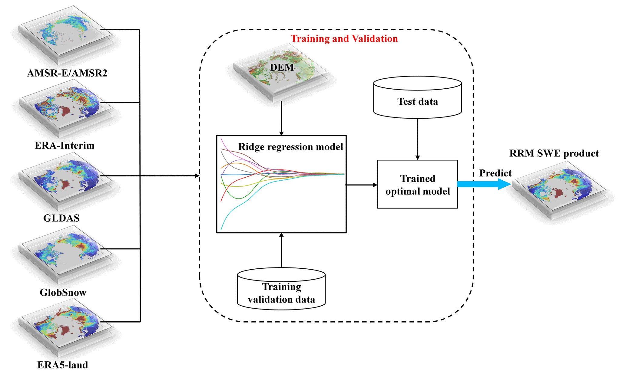
Figure 2Flow chart of the RRM SWE data preparation (preparation of spatiotemporal seamless SWE datasets mainly includes three processes: model training, model reasoning, and SWE data preparation).
2.4 Site data and evaluation metrics
2.4.1 Site SWE data for training, validation, and testing
Russian snow survey data (http://aisori.meteo.ru, last access: 17 February 2022) include the average snow depth data and the average snow density data of the station, and the SWE is the product of the measured average snow depth and average snow density (Bulygina et al., 2011). We obtained SWE data from 19 493 stations from 1979 to 2016 from this dataset.
Hemispheric-scale snow course (hereafter referred to as HSSC) observational data are contained in a hemispheric-scale SWE database based on SWE observational datasets from the former Soviet Union/Russia (FSU), Finland, and Canada developed by Pulliainen et al. (2020) (Bronnimann et al., 2018; Brown et al., 2019). This dataset is from the website of the Finnish Meteorological Institute (FMI) (https://www.globsnow.info/swe/archive_v3.0/auxiliary_data/, last access: 17 February 2022). The dataset provides data from 2687 distributed regional snow course observations and contains 343 241 SWE observational data points from 1979 to 2018. The snow courses of the HSSC dataset are transects in which SWE is sampled manually at multiple locations with typical conditions to eliminate uncertainty in the regional-scale spatial variability in SWE due to the influence of snowpack characteristics and land cover type (Pulliainen et al., 2020).
We carefully screened the Russian snow survey data and HSSC data and eliminated some abnormal observational data to ensure the high quality of the training, validation, and test sets. The null and zero values are removed during the HSSC data screening process. The null values, negative numbers, and extreme SWE values greater than 2000 mm are removed during the Russian snow survey data screening process.
2.4.2 Accuracy evaluation method for datasets
Mean absolute error (MAE), root mean square error (RMSE), Pearson's correlation coefficient (R), and coefficient of determination (R2) are used to evaluate the accuracies of AMSR-E/AMSR2 SWE, ERA-Interim SWE, GLDAS SWE, GlobSnow SWE, ERA5-Land SWE, multisource data-averaged SWE, and the RRM SWE product. The specific equations of accuracy evaluation error are described as follows:
where n is the number of samples in the validation dataset, fi is the SWE dataset product, yi is the measured SWE at the station, and are the averages of SWE products and measured SWEs, respectively, and σf and σy are the standard deviation of SWE products and measured SWEs, respectively.
To further evaluate the accuracy of the RRM SWE dataset at the spatial scale, we compared it with AMSR-E/AMSR2 SWE, ERA-Interim SWE, GLDAS SWE, GlobSnow SWE, and ERA5-Land SWE at different altitude gradients. We also evaluated MAE, RMSE, R, and R2 separately for 11 elevation intervals: <100, 100–200, 200–300, 300–400, 400–500, 500–600, 600–700, 700–800, 800–900, 900–1000, and >1000 m. In addition, we evaluated the performances of the RRM SWE product in three representative regions: Russia, Canada, and Finland.
We used the Mann–Kendall trend test (Mann, 1945; Kendall, 1990) method to evaluate the variation trend in the RRM SWE dataset from 1979 to 2019 and analyzed its reliability in terms of time series. Since the AMSR-E/AMSR2 SWE product and the GlobSnow SWE product lack SWE data for Greenland, we removed the Greenland data to maintain consistency in the spatial extent of the comparison data.
3.1 Overall accuracy evaluation of the RRM SWE product
In this study, the accuracies of the RRM SWE, AMSR-E/AMSR2 SWE, ERA-Interim SWE, GLDAS SWE, GlobSnow SWE, and ERA5-Land SWE were compared using test datasets from 2015 to 2018. MAE, RMSE, R, and R2 were used to reflect the data quality of each SWE product. In addition, we compared the RRM SWE product with the SWE dataset obtained by the multisource data average method.
According to the verification results in Fig. 3 and Table 2, the RRM SWE data have the best overall accuracy, and the MAE, RMSE, R, and R2 between the observed SWEs are 0.21, 25.37 mm, 0.89, and 0.79, respectively. The overall accuracy of the GlobSnow SWE and ERA5-Land SWE products is higher than that of other SWE products. The overall deviation of the ERA5-Land SWE products is the smallest except for the RRM SWE data, with MAE and RMSE values of 0.32 and 37.02 mm, respectively. The correlation between the ERA5-Land SWE and observed SWE is the highest except for the RRM SWE data, with R and R2 values of 0.84 and 0.71, respectively. Although the overall deviation between the GlobSnow SWE dataset and the measured SWE is small, its correlation with the measured value is low. The overall deviation between the ERA5-Land SWE dataset and the measured SWE is higher than that of the GlobSnow SWE dataset, but its estimation accuracy for the high-value region of the SWE is low. In addition, the overall accuracy of the ERA-Interim SWE dataset and GLDAS SWE dataset is relatively low, but their integrities are higher than those of the GlobSnow SWE dataset and AMSR-E/AMSR2 SWE dataset in terms of temporal and spatial series. The AMSR-E/AMSR2 SWE dataset has a higher estimation accuracy for the low-value SWE region. Moreover, in the land region above 45∘ N, most of the existing SWE data products with regard to temporal and spatial degrees are missing to various degrees. Obviously, the accuracies of the existing SWE products were uneven as no type of SWE dataset is perfect.
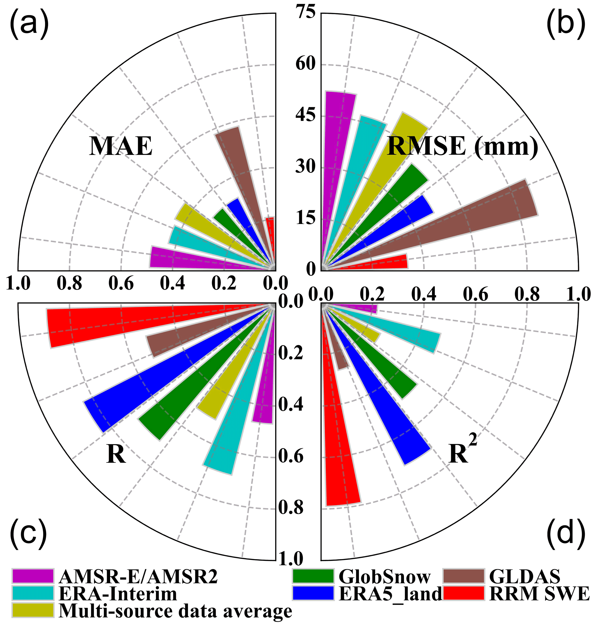
Figure 3Accuracy comparison of various SWE products. Sector (a) represents the MAE, sector (b) represents the RMSE, sector (c) represents R, and sector (d) represents R2. The sector axis represents the size of the error, and the color represents different SWE datasets.
Table 2Error list for the station data and grid snow water equivalent products.
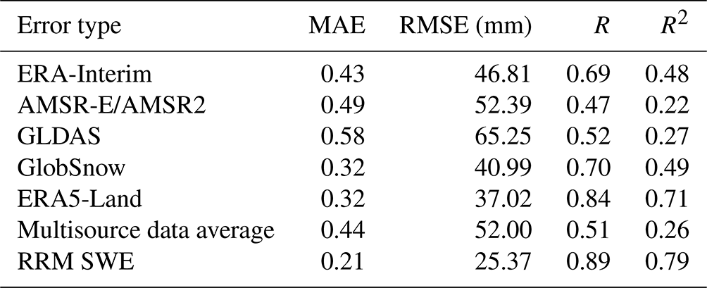
The verification results also indicate the following ranking orders.
The MAE ranking order is RRM SWE < GlobSnow SWE = ERA5-Land SWE < ERA-Interim SWE < multisource data average SWE < AMSR-E/AMSR2 SWE < GLDAS SWE.
The RMSE ranking order is RRM SWE < ERA5-Land SWE < GlobSnow SWE < ERA-Interim SWE < multisource data average SWE < AMSR-E/AMSR2 SWE < GLDAS SWE.
The R ranking order is RRM SWE > ERA5-Land SWE > GlobSnow SWE > ERA-Interim SWE > GLDAS SWE > multisource data average SWE > AMSR-E/AMSR2 SWE.
The R2 ranking order is RRM SWE > ERA5-Land SWE > GlobSnow SWE > ERA-Interim SWE > GLDAS SWE > multisource data average SWE > AMSR-E/AMSR2 SWE.
Compared with the ERA-Interim SWE, AMSR-E/AMSR2 SWE, GLDAS SWE, GlobSnow SWE, ERA5-Land SWE, and multisource data average SWE, the MAE of the RRM SWE and observed SWE is reduced by 0.22, 0.28, 0.37, 0.11, 0.11, and 0.23, respectively. The RMSE of the RRM SWE and observed SWE is reduced by 21.44, 27.02, 39.88, 15.62, 11.65, and 26.63 mm, respectively. The correlation coefficients of the RRM SWE and observed SWE are improved by 0.20, 0.42, 0.37, 0.19, 0.05, and 0.38, respectively. The coefficient of determination of the RRM SWE and observed SWE is improved by 0.31, 0.57, 0.52, 0.30, 0.08, and 0.53, respectively. Although the multisource data average method can improve the accuracy of SWE products to some extent (better than AMSR-E/AMSR2 SWE and GLDAS SWE), the improvement of this method is still very limited. The RRM SWE product has a significant advantage over the multisource data average method, and its accuracy is much higher than that of the simple multisource data average method (Table 2). Based on the above verification results, the accuracy of the RRM SWE is significantly improved; the RRM SWE dataset has higher accuracy than that of any single grid SWE dataset, and it also fills the gap in the original SWE data in terms of spatial and temporal resolutions.
Based on the kernel density estimation method, we analyzed the density distribution of different SWE datasets (Fig. 4). The results show that the RRM SWE dataset is closer to the 1:1 line and has the highest accuracy. The RRM SWE dataset is particularly accurate for SWE estimation in the low-value region, and the test data are concentrated near the 1:1 line in the high-density region (kernel density estimation >0.00015) (Fig. 4). In contrast, the high-density regions of the GLDAS SWE dataset, ERA-Interim SWE dataset, and AMSR-E/AMSR2 SWE dataset deviate significantly from the 1:1 line, resulting in poor accuracy. The AMSR-E/AMSR2 SWE, GLDAS SWE, and GlobSnow SWE are underestimated relative to the SWE measured at the site, among which GLDAS SWE underestimated the observed SWE the most seriously, while ERA5-Land SWE overestimated the observed SWE. Although the accuracies of GlobSnow SWE and ERA5-Land SWE are relatively high, their dispersion degrees are large (the kernel density estimation for most test data is less than 0.0001). Overall, the RRM SWE data have a higher overall estimation accuracy, especially for the low-value area of SWE. For an SWE above 400 mm, the MAE and RMSE of the RRM SWE product and the measured SWE are 0.35 and 43.57 mm, respectively. The estimation accuracy of the RRM SWE product for the high-value range of SWE (SWE>400 mm) is lower than that for the low-value range of SWE (SWE<400 mm) (Fig. 4). The main reason for this is that the training accuracy of the RRM model for the high-value range of SWE is affected by the small number of stations that observe the high-value range of SWE.
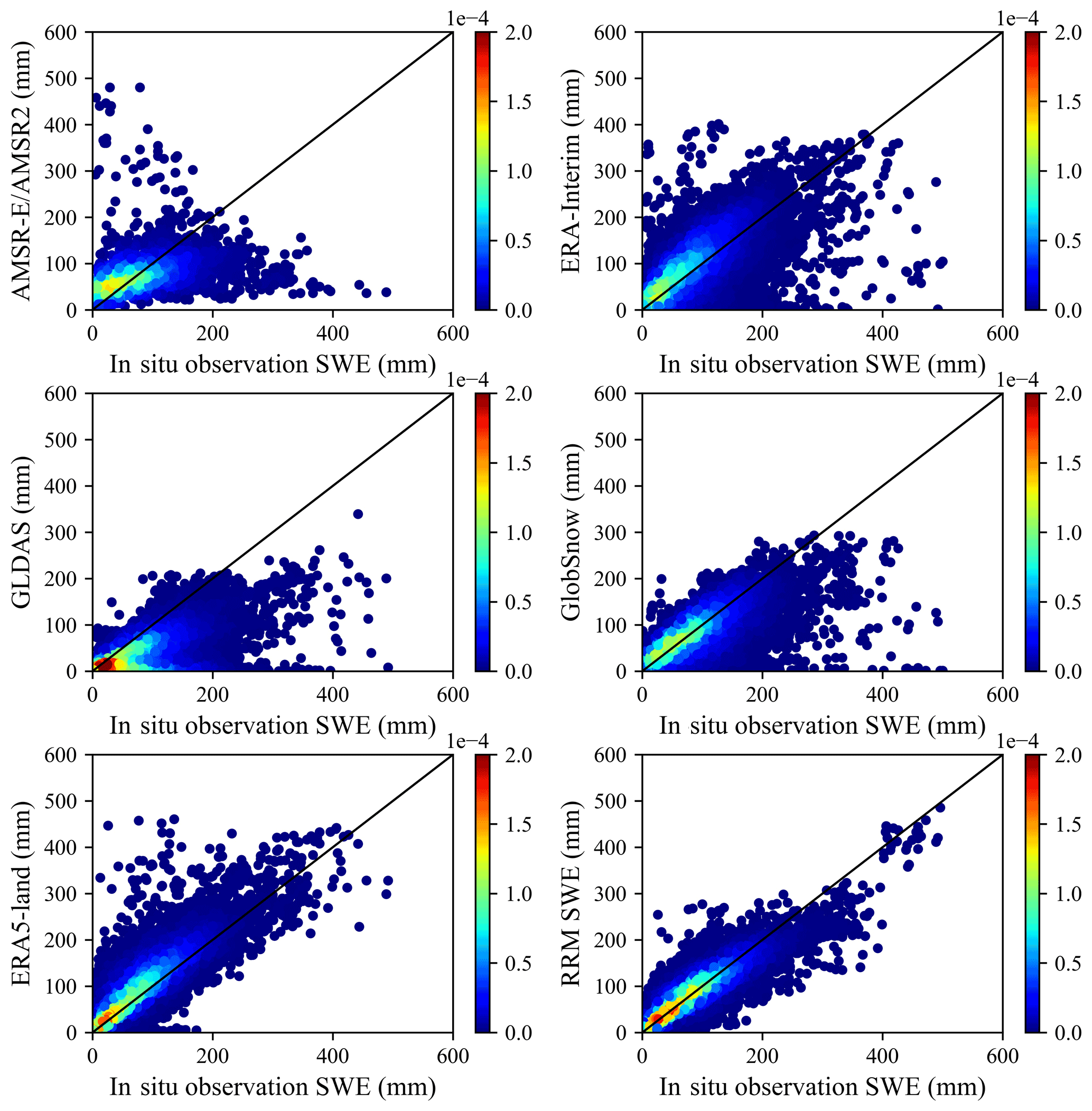
Figure 4Error verification density diagram (a total of 38 807 sample points were used for verification). The color bar represents the value of kernel density estimation. The closer the high-density area is to the 1:1 line, the higher the verification accuracy of the dataset is at most of the measuring stations.
However, in this study, there are still some uncertainties in the ridge regression machine learning algorithm that integrates SWE products. First, this model is strongly dependent on on-site observational data, and the fusion precision of SWE is poor in some areas with sparse observational stations. The fusion accuracy of SWE products will be affected to a certain extent without considering the prior snow cover information. The RRM SWE product is still underestimated in cases of high SWE. Then, in addition to the DEM, meteorological elements, Normalized Difference Vegetation Index (NDVI), land type, and other factors will affect the SWE estimation. Unfortunately, our current RRM presented here does not consider these factors as predictors, which is a limitation of the current RRM SWE product. Finally, in complex terrain with an elevation interval >1000 m, the RRM SWE product performed poorly, with an RMSE of 31.14 mm (Fig. 5), and the integration of SWE products remains challenging (Mortimer et al., 2020).
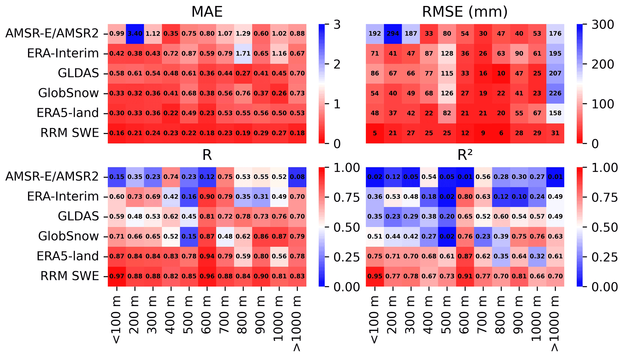
Figure 5Comparison of the error between the RRM SWE and AMSR-E/AMSR2 SWE, ERA-Interim SWE, GLDAS SWE, GlobSnow SWE, and ERA5-Land SWE at different altitudes (the abscissa represents the altitude gradient, and the ordinate represents different SWE datasets). The color bar indicates the error in each SWE dataset. The closer to red the color is, the higher the accuracy is. MAE: mean absolute error; RMSE: root mean square error; R: Pearson's correlation coefficient; R2: coefficient of determination.
3.2 Accuracy evaluation of the RRM SWE product at different altitudes and regions
The accuracy of each SWE product is not absolute at different altitude gradients based on evaluations of the AMSR-E/AMSR2 SWE, ERA-Interim SWE, GLDAS SWE, GlobSnow SWE, and ERA5-Land SWE product accuracies (Fig. 5). The accuracy of a single SWE product is different from its overall accuracy. We consider the influence of altitude in the algorithm and make full use of the accuracy advantage of each SWE data for different altitude gradients.
The above verification results show that the MAE, RMSE, R, and R2 between the RRM SWE product and measured SWE perform well at altitude gradients of <100, 100–200, 200–300, 300–400, 400–500, 500–600, 600–700, 700–800, 800–900, 900–1000, and >1000 m (Fig. 5). Overall, the RRM SWE product has the highest accuracy in the elevation intervals of <100, 100–200, 200–300, 400–500, 500–600, 600–700, 700–800, 800–900, and >1000 m. The RRM SWE product itself has the best performance in the elevation interval <100 m. The ERA5-Land product has the best performance in the elevation interval 300–400 m. The GlobSnow product has the best performance in the elevation interval 900–1000 m.
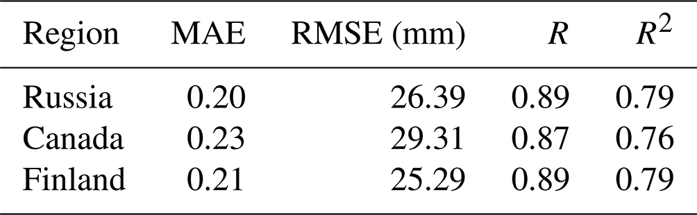
The RRM SWE product has good performance in different regions, and its RMSEs in Russia, Canada, and Finland are 26.39, 29.31, and 25.29 mm, respectively; additionally, the performance of the RRM SWE product in different regions is basically similar (Table 3). The RRM SWE product performs well not only at different altitudes but also in different regions, and it has good stability.
Table 3Error list for the station data and RRM SWE product in different regions.
3.3 Comparison of spatial distribution patterns between the RRM SWE product and traditional SWE products
A comparison of the spatially distributed annual average SWE distributions is made between the RRM SWE and AMSR-E/AMSR2 SWE, ERA-Interim SWE, GLDAS SWE, GlobSnow SWE, and ERA5-Land SWE in 2014, 2015, 2016, and 2017, and their spatial distribution patterns are shown in Fig. 6.
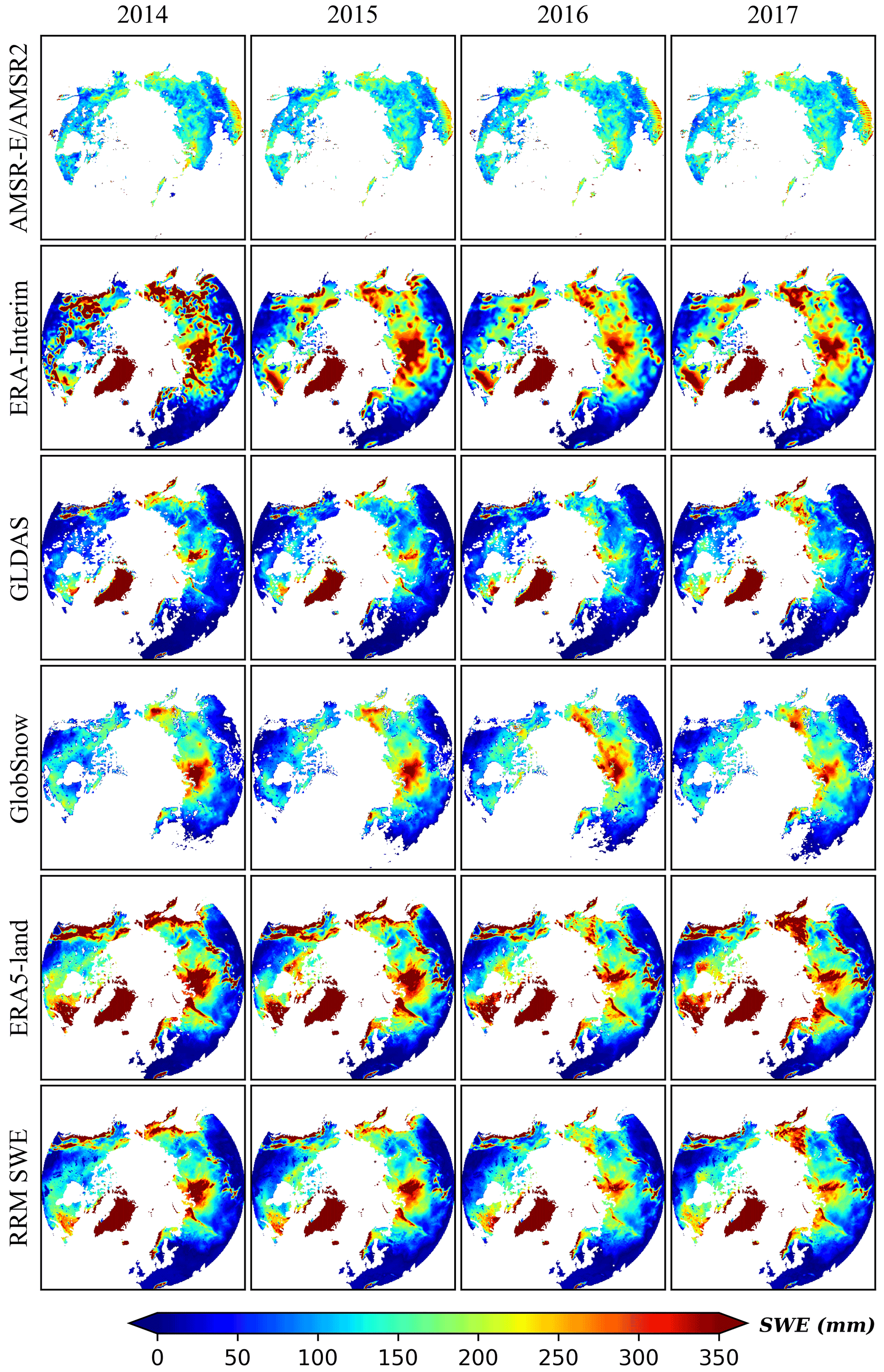
Figure 6Comparison of the spatial distribution characteristics between the RRM SWE and AMSR-E/AMSR2 SWE, ERA-Interim SWE, GLDAS SWE, GlobSnow SWE, and ERA5-Land SWE (the four columns of images represent the comparison results in 2014, 2015, 2016, and 2017).
Overall, the RRM SWE dataset, AMSR-E/AMSR2 SWE dataset, ERA-Interim SWE dataset, GLDAS SWE dataset, GlobSnow SWE dataset, and ERA5-Land SWE dataset have similar spatial distribution patterns in the land region above 45∘ N, showing a trend of lower SWE at low latitudes and higher SWE at high latitudes. The AMSR-E/AMSR2 SWE dataset covers a limited extent in the land region above 45∘ N, many data points are missing, and low SWE values exist at low latitudes. In northern Siberia, the ERA-Interim SWE product has a higher SWE, and there are many abnormal, extreme SWE values (SWE>500 mm) in this dataset. In low-latitude regions, such as Alaska, northern Siberia, and the easternmost region of Russia, the SWE of GLDAS SWE products is significantly lower. The GlobSnow SWE product lacks SWE data for Greenland, and this dataset has low SWEs in the regions of Baffin Island, Koryak Mountains, Kamchatka Peninsula, and Alaska. The ERA5-Land SWE products have low SWEs in northeastern Russia, Scandinavia, and northeastern Canada. The RRM SWE dataset is more reasonable for estimating the spatial distribution of SWE in the land region above 45∘ N, and the data integrity is higher. Moreover, based on the new machine learning algorithm, a variety of SWE data products in different time series are fused, which makes the RRM SWE dataset completely temporally and spatially continuous.
The relative difference between the RRM SWE data and GLDAS SWE data is the highest, and the relative difference is greater than 80 % in most low altitude regions (Fig. 7). The relative difference between the RRM SWE data and the GlobSnow SWE data is relatively small overall, especially in most high-latitude areas where the relative difference is less than 10 % (Fig. 7). Overall, the annual average relative differences in the RRM SWE data and AMSR2 SWE, ERA-Interim SWE, GLDAS SWE, GlobSnow SWE, and ERA5-Land SWE are 37 %, 41 %, 54 %, 25 %, and 29 %, respectively (Fig. 7). Previous studies have shown that the accuracy of the SWE in the Northern Hemisphere estimated by GlobSnow SWE data is higher (Pulliainen et al., 2020), while the spatial distribution pattern of the RRM SWE data is close to the estimation result of GlobSnow SWE. In addition, the single point verification results based on the measured SWE data of meteorological stations in Sect. 3.1 show that the RRM SWE dataset has higher accuracy than the GlobSnow SWE dataset. The RRM SWE dataset has good accuracy.
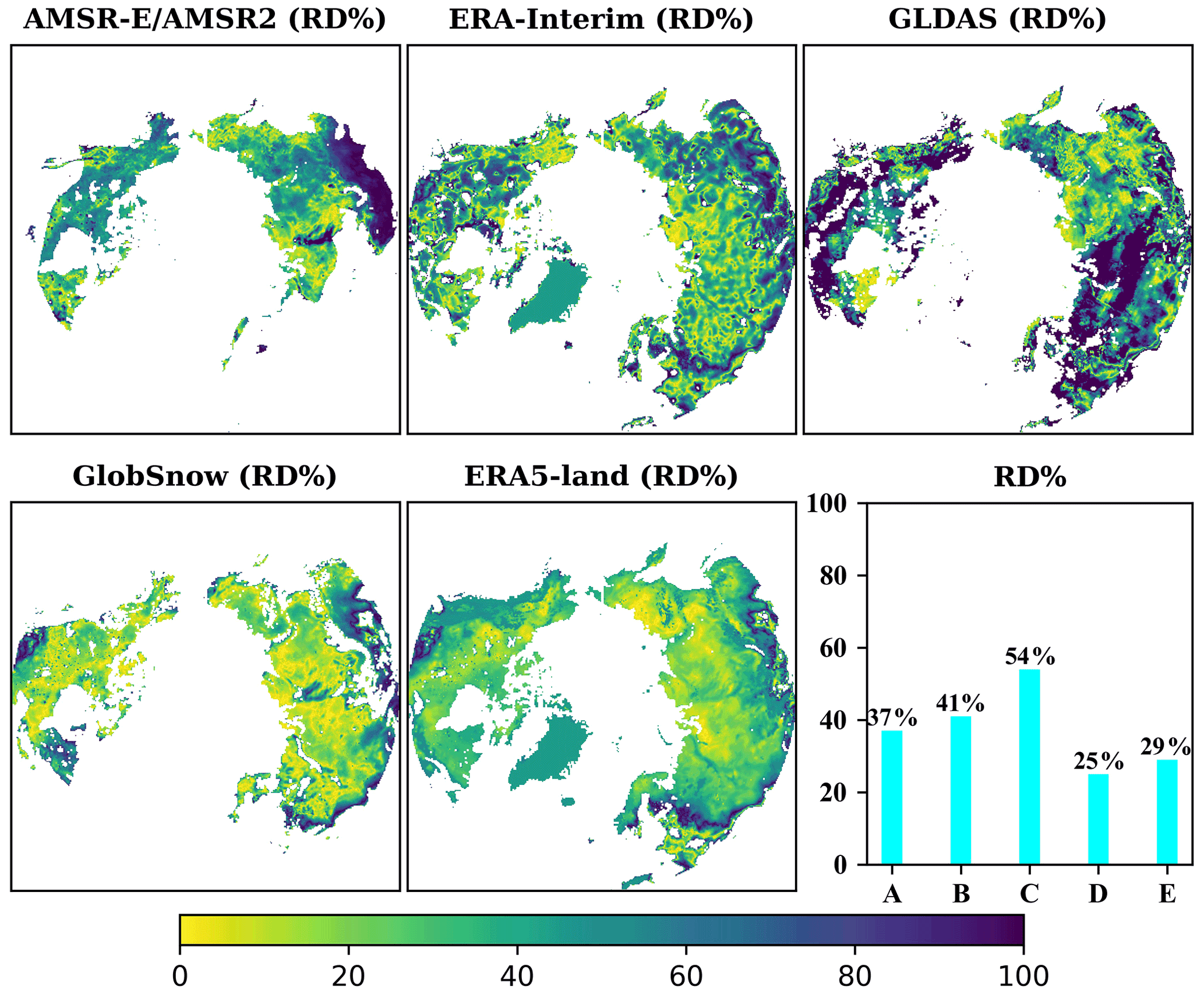
Figure 7Temporal and spatial distributions of relative differences (RD%) between the RRM SWE and AMSR-E/AMSR2 SWE, ERA-Interim SWE, GLDAS SWE, GlobSnow SWE, and ERA5-Land SWE. Lower-right panel: comparison of annual average relative differences between the RRM SWE and AMSR2 SWE (A), ERA-Interim SWE (B), GLDAS SWE (C), GlobSnow SWE (D), and ERA5-Land SWE (E).
3.4 Comparison of the annual variation tendencies of AMSR-E/AMSR2 SWE, ERA-Interim SWE, GLDAS SWE, GlobSnow SWE, and ERA5-Land SWE and the RRM SWE in the land region above 45∘ N
Based on the Mann–Kendall trend test, we analyzed the changing trend in the region-wide annual average SWE of the AMSR-E/AMSR2 SWE, ERA-Interim SWE, GLDAS SWE, GlobSnow SWE, ERA5-Land SWE, and RRM SWE in the land region above 45∘ N from 1979 to 2019.
Based on the Mann–Kendall trend test (see Fig. 8 and Table 4), from 1979 to 2019, the test value of the ERA-Interim region-wide annual average SWE is 1.08, and there is no significant change trend under the significance test level of 0.05. The test value of the GLDAS region-wide annual average SWE was 4.95 and showed a significant increasing trend at the significance test level of 0.05. The test values of the AMSR-E/AMSR2 annual average SWE, GlobSnow annual average SWE, ERA5-Land annual average SWE, and RRM annual average SWE are −3.26, −2.54, −3.43, and −3.00, respectively, and these four SWEs showed a significant decreasing trend at the significance test level of 0.05. Based on the analysis of the RRM SWE product, between 1979 and 2019, the region-wide annual average SWE in the land region above 45∘ N decreased by 15.1 %. In the Northern Hemisphere, spring snow cover extent has decreased significantly, according to the Fifth Assessment Report (AR5) of the IPCC. Between 1967 and 2010, the spring snow cover extent decreased by an average of 1.6 % per decade, while the June snow cover extent decreased by 11.7 % per decade (Stocker, 2014). Most studies have shown that the annual variation tendency of snow depth and snow cover extent showed a significant decreasing trend in the Northern Hemisphere (Brutel-Vuilmet et al., 2013), which is consistent with the annual variation tendency of the RRM SWE dataset. This dataset can reflect the characteristics of snow cover change in the land region above 45∘ N in light of climate change and can be used as the driving data for climate models to support climate-change-related research. In addition, this dataset is expected to provide a snow data basis for the study of “Arctic amplification”.

Figure 8Annual variation tendency of the AMSR-E/AMSR2 SWE, ERA-Interim SWE, GLDAS SWE, GlobSnow SWE, ERA5-Land SWE, and RRM SWE products from 1979 to 2019 (the dotted line is the trend line calculated based on the Mann–Kendall method).
Table 4Results of the Mann–Kendall trend test performed for various snow water equivalent products from 1979 to 2019.
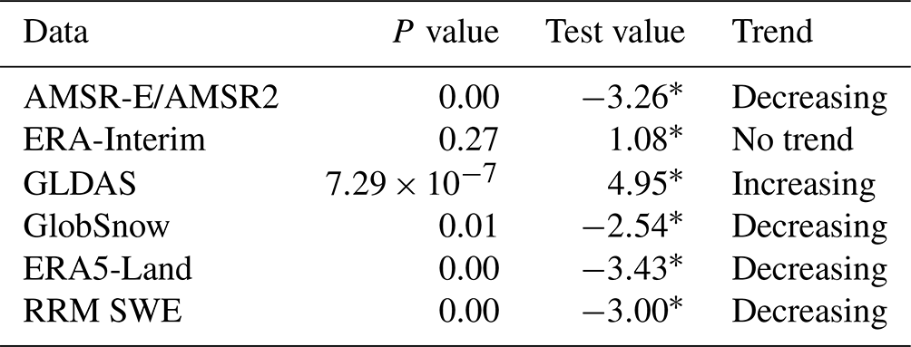
∗ Significance level alpha=0.05.
The RRM SWE product is available for free download from “A Big Earth Data Platform for Three Poles” (https://doi.org/10.11888/Snow.tpdc.271556, Li et al., 2021). The temporal resolution of the RRM SWE product is daily, and the spatial resolution is 10 km. It spans latitudes of 45–90∘ N and longitudes of 180∘ W–180∘ E. A brief summary and data description document (including data details, spatial range, and usage method) are also provided.
In this study, we propose a method to fuse multisource SWE data by a ridge regression model based on machine learning. A new method was utilized to prepare a set of spatiotemporally seamless SWE datasets of the RRM SWE, combined with the original AMSR-E/AMSR2 SWE, ERA-Interim SWE, GLDAS SWE, GlobSnow SWE, and ERA5-Land SWE datasets. In the RRM SWE dataset, the time series of the data is 1979–2019, the temporal resolution is daily, the spatial resolution is 10 km, and the spatial range is the land region above 45∘ N.
The RRM SWE data product has the best accuracy, especially for the estimation of low SWE. The accuracy ranking of the SWE dataset verified by the test dataset is described as follows: RRM SWE > ERA5-Land SWE > GlobSnow SWE > ERA-Interim SWE > multisource data average SWE > AMSR-E/AMSR2 SWE > GLDAS SWE. The accuracy of the RRM SWE dataset is higher than that of the existing SWE products at most elevation intervals. The RRM SWE product has good performance and stability in different regions. Moreover, the RRM SWE dataset spatiotemporally fills in the missing data of the original SWE dataset.
Compared with traditional fusion methods, machine learning methods have a strong advantage. We find that the simple machine learning algorithm has not only high efficiency but also good accuracy in the preparation of SWE products on a global scale. Without losing the advantages of existing SWE products, this method can also make full use of station observational data to integrate the advantages of various SWE products. The model training process does not rely too much on a specific sample, and this model has a strong generalization ability. In addition, the influence of altitude on the preparation scheme is considered in detail in the model. Compared with the SWE dataset prepared by the traditional method, the spatial resolution is only 25 km, while this new method obtains an SWE dataset with a higher spatial resolution of 10 km.
We propose that the RRM SWE dataset preparation scheme has good continuity and can prepare real-time and high-quality SWE datasets in the land region above 45∘ N. In addition, the new method proposed in this paper has the advantages of simplicity and high precision in preparing large-scale SWE datasets and can be easily extended to the preparation of other snow datasets. This dataset is an important supplement to the land region above the 45∘ N SWE database and is expected to provide data support for Arctic cryosphere studies and global climate change studies.
DS and HL designed the study and wrote the manuscript. JW, XH, and TC contributed to the discussions, edits, and revisions. DS and WJ compiled the model code.
The contact author has declared that neither they nor their co-authors have any competing interests.
Publisher's note: Copernicus Publications remains neutral with regard to jurisdictional claims in published maps and institutional affiliations.
This article is part of the special issue “Extreme environment datasets for the three poles”. It is not associated with a conference.
The authors would like to thank the European Space Agency (ESA) for providing the GlobSnow data, the European Centre for Medium-Range Weather Forecasts (ECMWF) for ERA-Interim data and ERA5-Land data, the National Aeronautics and Space Administration (NASA) for the AMSR-E/AMSR2 data, the Goddard Earth Sciences Data and Information Services Center (GES DISC) for the GLDAS data, the Russian Federal Service for Hydrometeorology and Environmental Monitoring (ROSHYDROMET) for the snow survey data, and the Finnish Meteorological Institute (FMI) for the hemispheric-scale snow course (HSSC) observational data.
This research has been supported by the Strategic Priority Research Program of the Chinese Academy of Sciences (grant no. XDA19070302), the National Science Fund for Distinguished Young Scholars (grant no. 42125604), and the National Natural Science Foundation of China (grant nos. 41971399, 41971325, 42171391).
This paper was edited by Baptiste Vandecrux and reviewed by two anonymous referees.
Bair, E. H., Abreu Calfa, A., Rittger, K., and Dozier, J.: Using machine learning for real-time estimates of snow water equivalent in the watersheds of Afghanistan, The Cryosphere, 12, 1579–1594, https://doi.org/10.5194/tc-12-1579-2018, 2018.
Balsamo, G., Albergel, C., Beljaars, A., Boussetta, S., Brun, E., Cloke, H., Dee, D., Dutra, E., Muñoz-Sabater, J., Pappenberger, F., de Rosnay, P., Stockdale, T., and Vitart, F.: ERA-Interim/Land: a global land surface reanalysis data set, Hydrol. Earth Syst. Sci., 19, 389–407, https://doi.org/10.5194/hess-19-389-2015, 2015.
Barnett, T. P., Adam, J. C., and Lettenmaier, D. P.: Potential impacts of a warming climate on water availability in snow-dominated regions, Nature, 438, 303–309, https://doi.org/10.1038/nature04141, 2005.
Bintanja, R. and Andry, O.: Towards a rain-dominated Arctic, Nat. Clim. Change, 7, 263–267, https://doi.org/10.1038/Nclimate3240, 2017.
Bronnimann, S., Allan, R., Atkinson, C., Buizza, R., Bulygina, O., Dahlgren, P., Dee, D., Dunn, R., Gomes, P., John, V. O., Jourdain, S., Haimberger, L., Hersbach, H., Kennedy, J., Poli, P., Pulliainen, J., Rayner, N., Saunders, R., Schulz, J., Sterin, A., Stickler, A., Titchner, H., Valente, M. A., Ventura, C., and Wilkinson, C.: Observations for Reanalyses, B. Am. Meteorol. Soc., 99, 1851–1866, https://doi.org/10.1175/Bams-D-17-0229.1, 2018.
Brown, R. D., Fang, B., and Mudryk, L.: Update of Canadian historical snow survey data and analysis of snow water equivalent trends, 1967–2016, Atmos.-Ocean, 57, 149–156, 2019.
Broxton, P. D., Van Leeuwen, W. J., and Biederman, J. A.: Improving snow water equivalent maps with machine learning of snow survey and lidar measurements, Water Resour. Res., 55, 3739–3757, 2019.
Brutel-Vuilmet, C., Ménégoz, M., and Krinner, G.: An analysis of present and future seasonal Northern Hemisphere land snow cover simulated by CMIP5 coupled climate models, The Cryosphere, 7, 67–80, https://doi.org/10.5194/tc-7-67-2013, 2013.
Bulygina, O. N., Groisman, P. Y., Razuvaev, V. N., and Korshunova, N. N.: Changes in snow cover characteristics over Northern Eurasia since 1966, Environ. Res. Lett., 6, 045204, https://doi.org/10.1088/1748-9326/6/4/045204, 2011.
Dee, D. P., Uppala, S. M., Simmons, A., Berrisford, P., Poli, P., Kobayashi, S., Andrae, U., Balmaseda, M., Balsamo, G., and Bauer, B, Beljaars, B. V., Bidlot, J., Bormann, N., Delsol, Dragani, R., Fuentes, M., and Vitart, F.: The ERA – Interim reanalysis: Configuration and performance of the data assimilation system, Q. J. Roy. Meteor. Soc., 137, 553–597, 2011.
Duzan, H. and Shariff, N. S. B. M.: Ridge regression for solving the multicollinearity problem: review of methods and models, J. Appl. Sci., 15, 392–404, https://doi.org/10.3923/jas.2015.392.404, 2015.
Friedman, J., Hastie, T., and Tibshirani, R.: Regularization Paths for Generalized Linear Models via Coordinate Descent, J. Stat. Softw., 33, 1–22, https://doi.org/10.18637/jss.v033.i01, 2010.
Gelaro, R., McCarty, W., Suarez, M. J., Todling, R., Molod, A., Takacs, L., Randles, C. A., Darmenov, A., Bosilovich, M. G., Reichle, R., Wargan, K., Coy, L., Cullather, R., Draper, C., Akella, S., Buchard, V., Conaty, A., da Silva, A. M., Gu, W., Kim, G. K., Koster, R., Lucchesi, R., Merkova, D., Nielsen, J. E., Partyka, G., Pawson, S., Putman, W., Rienecker, M., Schubert, S. D., Sienkiewicz, M., and Zhao, B.: The Modern-Era Retrospective Analysis for Research and Applications, Version 2 (MERRA-2), J. Climate, 30, 5419–5454, https://doi.org/10.1175/Jcli-D-16-0758.1, 2017.
Guilkey, D. K. and Murphy, J. L.: Directed Ridge Regression Techniques in Cases of Multicollinearity, J. Am. Stat. Assoc., 70, 769–775, 1975.
Henderson, G. R., Peings, Y., Furtado, J. C., and Kushner, P. J.: Snow-atmosphere coupling in the Northern Hemisphere, Nat. Clim. Change, 8, 954–963, https://doi.org/10.1038/s41558-018-0295-6, 2018.
Hoerl, A. E. and Kennard, R. W.: Ridge regression: applications to nonorthogonal problems, Technometrics, 12, 69–82, 1970a.
Hoerl, A. E. and Kennard, R. W.: Ridge regression: Biased estimation for nonorthogonal problems, Technometrics, 12, 55–67, 1970b.
Imaoka, K., Kachi, M., Fujii, H., Murakami, H., Hori, M., Ono, A., Igarashi, T., Nakagawa, K., Oki, T., Honda, Y., and Shimoda, H.: Global Change Observation Mission (GCOM) for Monitoring Carbon, Water Cycles, and Climate Change, P IEEE, 98, 717–734, https://doi.org/10.1109/Jproc.2009.2036869, 2010.
IPCC: Climate Change 2021: The Physical Science Basis. Contribution of Working Group I to the Sixth Assessment Report of the Intergovernmental Panel on Climate Change, edited by: Masson-Delmotte, V., Zhai, P., Pirani, A., Connors, S. L., Péan, C., Berger, S., Caud, N., Chen, Y., Goldfarb, L., Gomis, M. I., Huang, M., Leitzell, K., Lonnoy, E., Matthews, J. B. R., Maycock, T. K., Waterfield, T., Yelekçi, O., Yu, R., and Zhou, B., Cambridge University Press, https://www.ipcc.ch/report/ar6/wg1/downloads/report/IPCC_AR6_WGI_Full_Report.pdf (last access: 17 February 2022), in press, 2021.
Kelly, R.: The AMSR-E Snow Depth Algorithm: Description and Initial Results, J. Remote Sens. Soc. Jpn., 29, 307–317, https://doi.org/10.11440/rssj.29.307, 2009.
Kendall, M. G.: Rank Correlation Methods, Brit. J. Psychol., 25, 86–91, 1990.
Li, H., Shao, D., Li, H., Wang, W., Ma, Y., and Lei, H.: Arctic Snow Water Equivalent Grid Dataset (1979–2019), A Big Earth Data Platform for Three Poles [data set], https://doi.org/10.11888/Snow.tpdc.271556, 2021.
Luojus, K., Pulliainen, J., Takala, M., Lemmetyinen, J., Mortimer, C., Derksen, C., Mudryk, L., Moisander, M., Hiltunen, M., and Smolander, T.: GlobSnow v3.0 Northern Hemisphere snow water equivalent dataset, Sci. Data, 8, 1–16, 2021.
Mann, H. B.: Nonparametric test against trend, Econometrica, 13, 245–259, 1945.
Menne, M., Durre, I., Korzeniewski, B., McNeal, S., Thomas, K., Yin, X., Anthony, S., Ray, R., Vose, R., and Gleason, B.: Global Historical Climatology Network–Daily (GHCN-Daily), Version, 3, V5D21VHZ, https://doi.org/10.7289/V5D21VHZ, 2016.
Mortimer, C., Mudryk, L., Derksen, C., Luojus, K., Brown, R., Kelly, R., and Tedesco, M.: Evaluation of long-term Northern Hemisphere snow water equivalent products, The Cryosphere, 14, 1579–1594, https://doi.org/10.5194/tc-14-1579-2020, 2020.
Mudryk, L. R., Derksen, C., Kushner, P. J., and Brown, R.: Characterization of Northern Hemisphere Snow Water Equivalent Datasets, 1981–2010, J. Climate, 28, 8037–8051, https://doi.org/10.1175/Jcli-D-15-0229.1, 2015.
Muñoz Sabater, J.: ERA5-Land hourly data from 1981 to present, Copernicus Climate Change Service (C3S) Climate Data Store (CDS) [data set], https://doi.org/10.24381/cds.e2161bac, 2019.
Ntokas, K. F. F., Odry, J., Boucher, M.-A., and Garnaud, C.: Investigating ANN architectures and training to estimate snow water equivalent from snow depth, Hydrol. Earth Syst. Sci., 25, 3017–3040, https://doi.org/10.5194/hess-25-3017-2021, 2021.
Pan, M., Sheffield, J., Wood, E. F., Mitchell, K. E., Houser, P. R., Schaake, J. C., Robock, A., Lohmann, D., Cosgrove, B., and Duan, Q.: Snow process modeling in the North American Land Data Assimilation System (NLDAS): 2. Evaluation of model simulated snow water equivalent, J. Geophys. Res.-Atmos., 108, 8850, https://doi.org/10.1029/2003JD003994, 2003.
Pan, M., Fisher, C. K., Chaney, N. W., Zhan, W., Crow, W. T., Aires, F., Entekhabi, D., and Wood, E. F.: Triple collocation: Beyond three estimates and separation of structural/non-structural errors, Remote Sens. Environ., 171, 299–310, https://doi.org/10.1016/j.rse.2015.10.028, 2015.
Pulliainen, J.: Mapping of snow water equivalent and snow depth in boreal and sub-arctic zones by assimilating space-borne microwave radiometer data and ground-based observations, Remote Sens. Environ., 101, 257–269, https://doi.org/10.1016/j.rse.2006.01.002, 2006.
Pulliainen, J., Luojus, K., Derksen, C., Mudryk, L., Lemmetyinen, J., Salminen, M., Ikonen, J., Takala, M., Cohen, J., Smolander, T., and Norberg, J.: Publisher Correction: Patterns and trends of Northern Hemisphere snow mass from 1980 to 2018, Nature, 581, 294–298, https://doi.org/10.1038/s41586-020-2258-0, 2020.
Reichle, R. H., Koster, R. D., De Lannoy, G. J. M., Forman, B. A., Liu, Q., Mahanama, S. P. P., and Toure, A.: Assessment and Enhancement of MERRA Land Surface Hydrology Estimates, J. Climate, 24, 6322–6338, https://doi.org/10.1175/Jcli-D-10-05033.1, 2011.
Rodell, M., Houser, P., Jambor, U., Gottschalck, J., Mitchell, K., Meng, C.-J., Arsenault, K., Cosgrove, B., Radakovich, J., and Bosilovich, M.: The global land data assimilation system, B. Am. Meteorol. Soc., 85, 381–394, 2004.
Saleh, A. M. E., Arashi, M., and Kibria, B. G.: Theory of ridge regression estimation with applications, John Wiley & Sons, https://doi.org/10.1002/9781118644478, 2019.
Santi, E., Brogioni, M., Leduc-Leballeur, M., Macelloni, G., Montomoli, F., Pampaloni, P., Lemmetyinen, J., Cohen, J., Rott, H., Nagler, T., Derksen, C., King, J., Rutter, N., Essery, R., Menard, C., Sandells, M., and Kern, M.: Exploiting the ANN Potential in Estimating Snow Depth and Snow Water Equivalent From the Airborne SnowSAR Data at X-and Ku-Bands, IEEE T. Geosci. Remote, 1–16, https://doi.org/10.1109/TGRS.2021.3086893, 2021.
Snauffer, A. M., Hsieh, W. W., and Cannon, A. J.: Comparison of gridded snow water equivalent products with in situ measurements in British Columbia, Canada, J. Hydrol., 541, 714–726, https://doi.org/10.1016/j.jhydrol.2016.07.027, 2016.
Snauffer, A. M., Hsieh, W. W., Cannon, A. J., and Schnorbus, M. A.: Improving gridded snow water equivalent products in British Columbia, Canada: multi-source data fusion by neural network models, The Cryosphere, 12, 891–905, https://doi.org/10.5194/tc-12-891-2018, 2018.
Stocker, T.: Climate change 2013: the physical science basis: Working Group I contribution to the Fifth assessment report of the Intergovernmental Panel on Climate Change, Cambridge University Press, ISBN: 978-1-107-66182-0, https://www.ipcc.ch/site/assets/uploads/2017/09/WG1AR5_Frontmatter_FINAL.pdf (last access: 17 February 2022), 2014.
Tedesco, M. and Jeyaratnam, J.: AMSR-E/AMSR2 Unified L3 Global Daily 25 km EASE-Grid Snow Water Equivalent, Version 1, Boulder, Colorado USA, NASA National Snow and Ice Data Center Distributed Active Archive Center, https://doi.org/10.5067/8AE2ILXB5SM6, 2019.
Vuyovich, C. M., Jacobs, J. M., and Daly, S. F.: Comparison of passive microwave and modeled estimates of total watershed SWE in the continental United States, Water Resour. Res., 50, 9088–9102, 2014.
Walker, A., Brasnett, B., and Brown, R.: Canadian Meteorological Centre (CMC) daily gridded snow depth analysis for Northern Hemisphere, 1998–2008 [data set], https://doi.org/10.5443/10916, 2011.
Wang, J. W., Yuan, Q. Q., Shen, H. F., Liu, T. T., Li, T. W., Yue, L. W., Shi, X. G., and Zhang, L. P.: Estimating snow depth by combining satellite data and ground-based observations over Alaska: A deep learning approach, J. Hydrol., 585, 124828, https://doi.org/10.1016/j.jhydrol.2020.124828, 2020.
Xiao, X. X., Zhang, T. J., Zhong, X. Y., Shao, W. W., and Li, X. D.: Support vector regression snow-depth retrieval algorithm using passive microwave remote sensing data, Remote Sens. Environ., 210, 48–64, https://doi.org/10.1016/j.rse.2018.03.008, 2018.