the Creative Commons Attribution 4.0 License.
the Creative Commons Attribution 4.0 License.
 | 21 Dec 2022
A global dataset of daily maximum and minimum near-surface air temperature at 1 km resolution over land (2003–2020)
Tao Zhang
Kaiguang Zhao
Zhengyuan Zhu
Gang Chen
Jia Hu
Li Wang
Near-surface air temperature (Ta) is a key variable in global climate studies. A global gridded dataset of daily maximum and minimum Ta (Tmax and Tmin) is particularly valuable and critically needed in the scientific and policy communities but is still not available. In this paper, we developed a global dataset of daily Tmax and Tmin at 1 km resolution over land across 50∘ S–79∘ N from 2003 to 2020 through the combined use of ground-station-based Ta measurements and satellite observations (i.e., digital elevation model and land surface temperature) via a state-of-the-art statistical method named Spatially Varying Coefficient Models with Sign Preservation (SVCM-SP). The root mean square errors in our estimates ranged from 1.20 to 2.44 ∘C for Tmax and 1.69 to 2.39 ∘C for Tmin. We found that the accuracies were affected primarily by land cover types, elevation ranges, and climate backgrounds. Our dataset correctly represents a negative relationship between Ta and elevation and a positive relationship between Ta and land surface temperature; it captured spatial and temporal patterns of Ta realistically. This global 1 km gridded daily Tmax and Tmin dataset is the first of its kind, and we expect it to be of great value to global studies such as the urban heat island phenomenon, hydrological modeling, and epidemic forecasting. The data have been published by Iowa State University at https://doi.org/10.25380/iastate.c.6005185 (Zhang and Zhou, 2022).
- Article
(4655 KB) - Full-text XML
-
Supplement
(1459 KB) - BibTeX
- EndNote


Near-surface air temperature (Ta) refers to the atmospheric temperature 1.5–2 m above surfaces, and it is an important variable for numerous applications, especially those pertinent to climate and environment change (Huang et al., 2019; Zhang et al., 2018), terrestrial hydrology and phenology (Lin et al., 2012; Ren et al., 2019), public health (Lan et al., 2010, 2022; Zhang et al., 2019), disease vector propagation (Lowen et al., 2007; Petrova and Russell, 2018; Wu et al., 2020), and epidemic forecasting (Verma et al., 2017; Connor et al., 1998). Ta generally varies across space and time dramatically due to the spatial heterogeneity and temporal dynamics of environmental factors such as solar radiation, wind speed, land cover, cloud cover, and vegetation phenology (Benali et al., 2012; Chen et al., 2015, 2021; Prihodko and Goward, 1997). At the global scale, a Ta dataset will be of limited or no use if it does not characterize and capture such fine spatial details and continuous temporal coverage. A high-/medium-resolution global Ta dataset at the daily interval is highly desirable.
Many global or regional Ta datasets have been previously published (Chen et al., 2021; Crespi et al., 2021; Fang et al., 2021; Hersbach et al., 2018; Hooker et al., 2018; Kalnay et al., 1996; MacDonald et al., 2020; Meyer et al., 2019; Nashwan et al., 2019; Oyler et al., 2015; Thornton et al., 2021; Werner et al., 2019); however, these have either coarse spatiotemporal resolutions or only cover specific regions (Table S3 in the Supplement). For example, some global Ta datasets have daily frequencies but at coarse spatial resolutions (e.g., 0.05∘ or even coarser) (Hersbach et al., 2018; Hooker et al., 2018; Kalnay et al., 1996); other Ta datasets with medium spatial resolutions (∼ 1 km) are only available for specific regions such as North America and mainland China (MacDonald et al., 2020; Oyler et al., 2015; Thornton et al., 2021; Chen et al., 2021). There are also several Ta datasets at even finer spatial resolutions but generated only for much smaller spatial regions (Crespi et al., 2021; Meyer et al., 2019; Nashwan et al., 2019; Werner et al., 2019). Despite the increasing need for a global daily Ta at finer resolutions (e.g., 1 km), such global products do not exist yet – a gap still not filled yet.
Methodologically speaking, a range of techniques have been proposed and applied to generate Ta products; the majority of them rely on combining weather station data and gridded auxiliary datasets to simply make spatial interpolation or build empirical predictive models (Chen et al., 2015; Goward et al., 1994; Hengl et al., 2012; Hou et al., 2013; Hrisko et al., 2020; Li and Zha, 2019; Li et al., 2018; Nemani and Running, 1989; Rao et al., 2019; Shen et al., 2020; Shi et al., 2017; Sun et al., 2005; Yoo et al., 2018; Zhu et al., 2013). Common spatial interpolation algorithms, such as inverse distance weighting (IDW), spline, and kriging, are unlikely to be applicable at the global scale, for example, due to the relative sparsity of weather stations and the high spatial heterogeneity of Ta (Chai et al., 2011; Dodson and Marks, 1997; Li and Heap, 2011; Stahl et al., 2006). Model-based approaches are often a better choice to capture the true spatial variability in Ta; these methods are roughly divided into three groups. The first is the temperature–vegetation index (TVX) method, which estimates Ta from the maximum normalized difference vegetation index (NDVI) based on the assumption that the canopy temperature over fully covered vegetation approximates near-surface Ta (Goward et al., 1994; Nemani and Running, 1989; Zhu et al., 2013). An apparent weakness of the TVX method is its large uncertainty or unsuitability for regions with low vegetation cover. The second group is the energy balance method, leveraging the explicit modeling of surface energy balance and the quantification of net radiation (e.g., the sum of sensible, soil, and latent heat fluxes) (Sun et al., 2005; Zhang et al., 2015). Energy-based methods are physically based, requiring detailed characterization of surface biophysical conditions and thereby making it difficult to implement for large areas due to the lack of such detailed biophysical parameters.
Of the three groups, the third category is statistical methods that estimate Ta via statistical relationships empirically calibrated between Ta and other covariates. Common algorithms used include geographically weighted regression (GWR), cubist, random forests, and deep learning, among others (Chen et al., 2015, 2021; Hooker et al., 2018; Li et al., 2018; Rao et al., 2019; Shen et al., 2020; Yoo et al., 2018). Compared to physical-based methods, statistical methods have fewer restrictions on data requirements and better applicability for large spatial extents (Noi et al., 2017). However, direct applications of common statistical methods often fail to capture and preserve relationships between Ta and auxiliary covariates (e.g., an unrealistically positive relationship between Ta and elevation), thereby leading to large uncertainties or even incorrect results. To overcome such drawbacks, we recently proposed a class of Spatially Varying Coefficient Models with Sign Preservation (SVCM-SP) (Kim et al., 2021; Zhang et al., 2022b), which can capture and preserve relationships between Ta and explanatory variables. The SVCM-SP algorithm was originally implemented for estimating Ta over mainland China, with significant improvement in terms of both accuracies and computational efficiency compared to alternative methods such as GWR (Zhang et al., 2022b). The potential of SVCM-SP as a routine algorithm to generate global Ta products is still untapped and addressed here.
Here we aim to generate a global dataset of daily maximum and minimum Ta (Tmax and Tmin) at 1 km resolution across 50∘ S–79∘ N from 2003 to 2020 by integrating ground-station-based Ta measurements and gridded satellite-observed covariates (i.e., digital elevation model, DEM; land surface temperature, LST). We employed our newly developed SVCM-SP algorithm that, for example, can preserve negative and positive relationships with elevation and LST, respectively. Zhang et al. (2022b) successfully estimated and validated gridded Ta using the SVCM-SP algorithm and demonstrated its novelty through the comparison with the GWR model, while in this study, we developed the global product of gridded Ta, performed extensive model calibration and accuracy assessment at the global scale, and provided details on accuracy and spatial and temporal patterns of the global gridded Ta. Our dataset aims to provide the first ever 1 km resolution daily maximum and minimum Ta dataset with a global coverage.
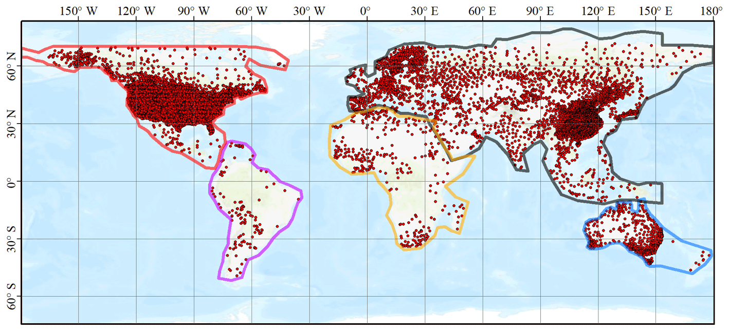
Figure 1Regions and locations of weather stations in this study. Red points are the locations of weather stations, and polygons are the boundaries of regions used in the SVCM-SP algorithm. Specifically, polygons of red, purple, orange, blue, and black represent the boundaries of North America, South America, Africa, Australia, and Europe and Asia, respectively.
Land areas covered by our global dataset span from 50∘ S to 79∘ N. We divided the global lands roughly into five regions: North America, South America, Europe and Asia, Africa, and Australia and New Zealand. To encompass all the land areas resolved at 1 km resolution, as well as to cover all the possible weather stations, the boundaries of the five regions were irregular. There also exist some overlaps between the regions. Our analysis considered three major data sources: ground-station-based Ta observations, satellite-derived LSTs, and elevation. In our algorithm, ground-station-based Ta is assumed to be statistically related to satellite LST and elevation. Details about each data source are further described below.
Ground-station-based daily Tmax and Tmin were compiled from a total of 103 156 weather stations from 2003 to 2020. These are obtained from two climatology networks: the Global Historical Climatology Network daily (GHCNd) across the world and the China Meteorological Data Service Centre (CMDC) across mainland China. The LST dataset is a global seamless 1 km resolution LST dataset at a daily (mid-daytime and mid-nighttime) frequency from 2003 to 2020, which was gap-filled from the MODIS LST products (Zhang et al., 2022a). Both the mid-daytime and mid-nighttime LSTs were considered in our analysis. The DEM layer we used is the SRTM30_PLUS product at 1 km resolution (Becker et al., 2009), which has been generated from the combination of the Shuttle Radar Topography Mission (SRTM30) topography (collected in 2000) (Hennig et al., 2001; Rosen, 2000) within a latitude of ± 55∘, ICESat-derived topography (collected from 1 February 2003 to 30 June 2005) (Dimarzio et al., 2007) in Antarctica, and the GTOPO30 topography (completed in late 1996) (Danielson and Gesch, 2011) in the Arctic. Besides, the Köppen–Geiger climate zones and MODIS land cover data (MCD12Q1) were acquired to divide the world into zones for accuracy assessment (Sulla-Menashe and Friedl, 2018). Specifically, our dataset covers a small portion of Greenland which is constrained by the extent of the global seamless 1 km daily LST dataset.
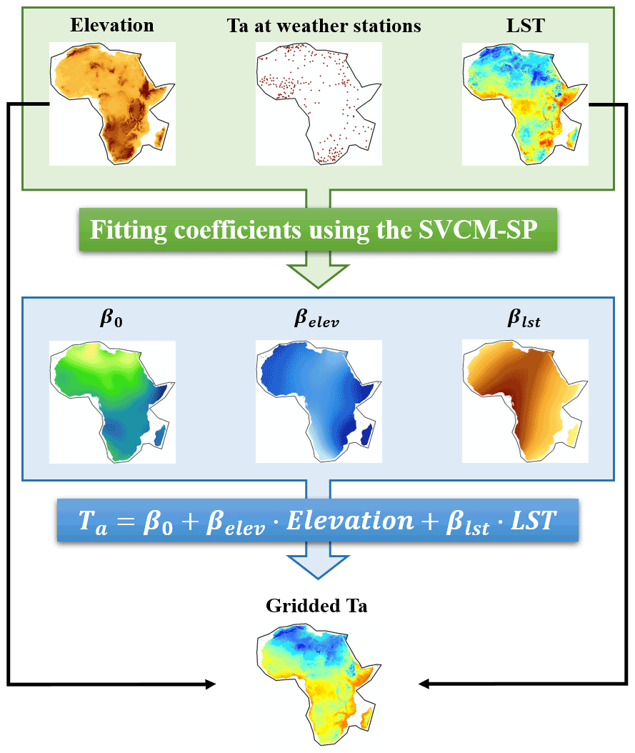
Figure 2Framework for implementing the SVCM-SP algorithm in a region (e.g., Africa). β0, βelev, and βlst are the intercept, coefficients of elevation, and LST, respectively.
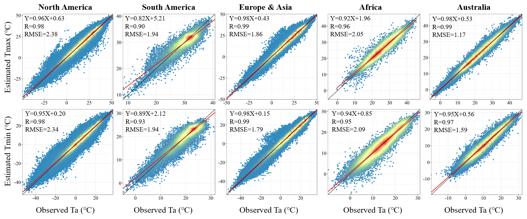
Figure 3Scatter plots between estimated and observed Ta in five regions in the year 2010. Each point represents the estimated and observed Ta (Tmax or Tmin) on a specific day at a weather station. The color of points represents the density, in which red and blue points represent the high and low densities, respectively. The red line is the regression line, and the black line is the 1:1 line.
The core of our methodological framework is the SVCM-SP algorithm that correlates ground-station-based Ta with satellite LST and elevation. We applied the SVCM-SP algorithm to estimate Tmax and Tmin separately. To capture potential non-stationarity, the algorithm was trained for each day of the period 2003–2020, as well as for each of the five regions. Before applying the SVCM-SP algorithm, weather station Ta data were first pre-processed and filtered for quality control to ensure the high fidelity of reference Ta observations.
Table 1Multi-year average accuracies for Tmax and Tmin in different regions from 2003 to 2020.
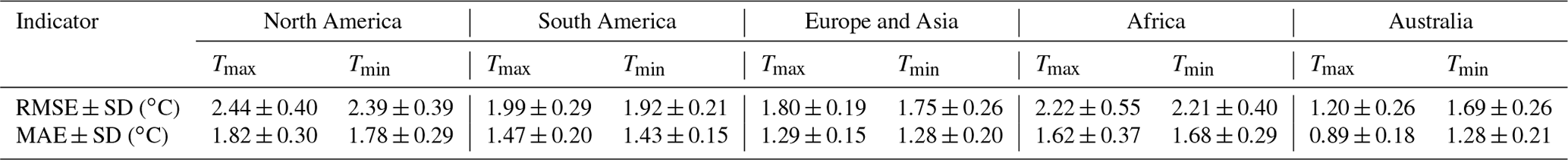
Note: the selected testing stations were within 50 km surrounding the training stations. SD represents the corresponding standard deviation.
Table 2Model performance for different land cover types in 2003–2020.
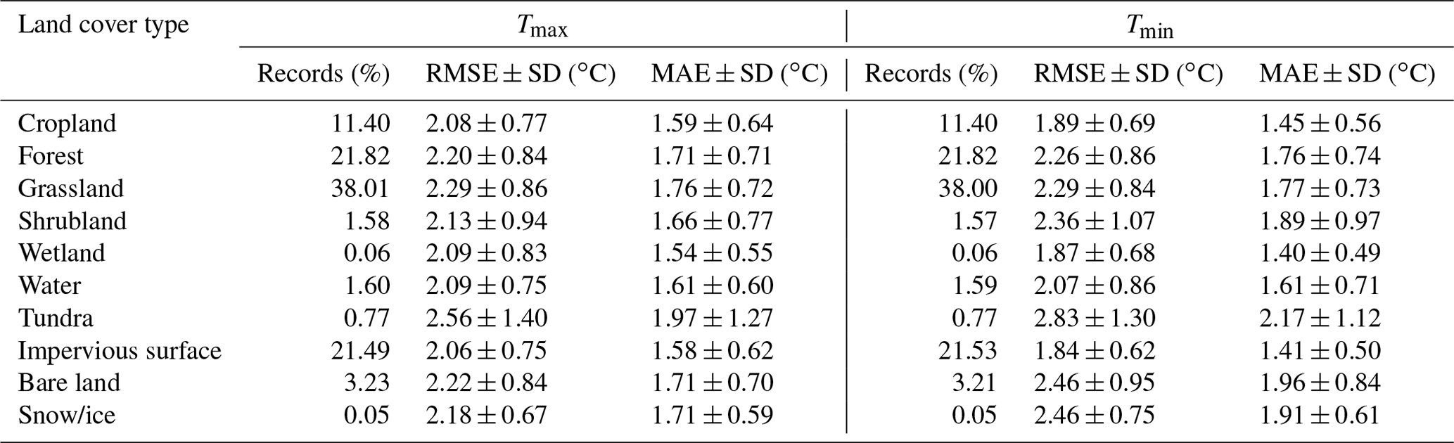
Note: SD represents the corresponding standard deviation.
Table 3Model performance for different elevation ranges in 2003–2020.
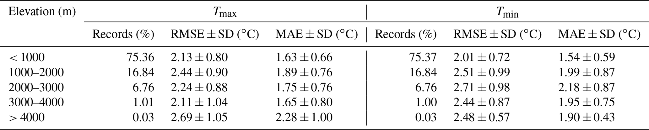
Note: SD represents the corresponding standard deviation.
More specially, we first processed the weather station data in three ways. First, the locations of many weather stations in China, especially those located in complex terrains, are not accurately documented, geo-referenced only at the level of arc degrees and minutes in the metadata. Such location errors have to be corrected, and we manually corrected the locations of those weather stations located over complex terrains by searching the meteorological observation fields near the reported locations of weather stations with the help of high-spatial-resolution images from ArcGIS base map or Google Maps (Zhang et al., 2022b). Second, there are missing values, especially in stations in Africa and South America (Fig. S1 in the Supplement). We filled these data gaps using a 5 d local moving window (Fig. S2 in the Supplement). Accordingly, the number of records largely increased (Figs. S3 and S4 in the Supplement) with reasonable error ranges (Fig. S5 in the Supplement). Third, the processed ground-station-based Ta data from the two steps were overlaid and matched with satellite LST and elevation to extract pairs of ground-station-based Ta and satellite covariates as inputs to the SVCM-SP algorithm. Specifically, mid-daytime and mid-nighttime LSTs were used to develop their relationship with air temperature to interpolate station Tmax and Tmin, respectively. The actual time of Tmax and Tmin may be slightly different from mid-daytime and mid-nighttime LSTs. Within the small difference in time between LST and , there will not be significant change in the spatial variations in LST. Therefore, the impact of time difference between LST and on the accuracy of the estimated Ta is minor as shown by shifting LST for time difference (Fig. S8 in the Supplement).
The SVCM-SP algorithm seeks to build a spatially varying relationship between ground-station-based Ta with LST and elevation with sign preservation (Kim et al., 2021; Zhang et al., 2022b). A salient feature distinguishing it from conventional regression approaches is the spatially varying nature with constraints of estimated coefficients in the predictive relationship:
where both the variables (e.g., Ta, elevation, and LST) and the model parameters are functions of locations/coordinates (uivi). More importantly, the two slope parameters (e.g., βelev and βlst) are constrained to be negative and positive, respectively. εi is the normal random error with mean zero and finite variance. These unknown parameters were estimated with a penalized bivariate spline method based on the triangulation technique under constraints. Details about the SVCM-SP algorithm are reported in Kim et al. (2021) and Zhang et al. (2022b). To estimate Ta across the globe, we applied the SVCM-SP algorithm to develop region-specific relationships for the five regions (Fig. 2). Also, two separate sets of equations were developed, one for Tmax using mid-daytime LST as the explanatory variable, and another for Tmin using midnight LST as the explanatory variable. The model performance for estimating gridded Ta was assessed based on root mean square error (RMSE) and mean square error (MAE) using the 10-fold cross-validation in these regions in each day. Taking the RMSE as an example, a RMSE was generated in each test of the 10-fold cross-validation, and all RMSEs from the 10 tests were averaged as the final RMSE on a specific day in a specific region. This accuracy assessment using the 10-fold cross-validation was implemented based on independent validation data and can provide a reliable evaluation of the accuracy. For each station, we can also calculate RMSE based on the time series of estimated and validation Ta from the 10-fold cross-validation. Accordingly, we can calculate mean RMSE and corresponding standard deviation in each land cover type, climate type, and elevation range. Specifically, this accuracy assessment represents conservative estimates of the uncertainties of our data because when producing the final results, we used all the available data, more than those in the 10-fold cross-validation.
Table 4Model performance for different climate types in 2003–2020.
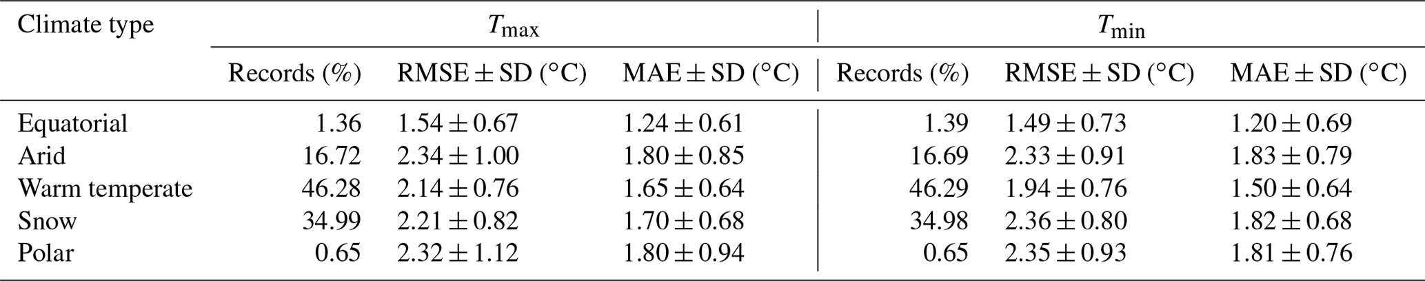
Note: SD represents the corresponding standard deviation.
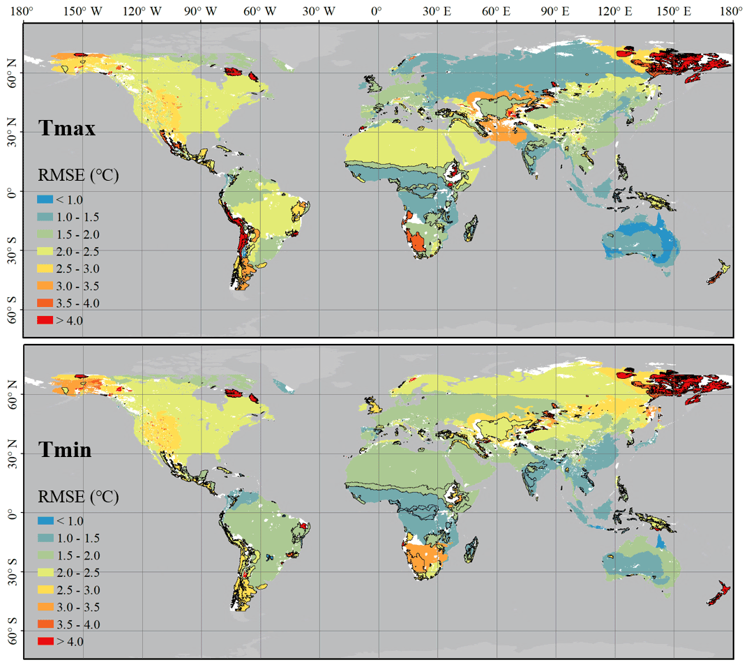
Figure 4Accuracy of estimated Ta in climate zones in 2003–2020. Climate zones with black boundaries are areas with low densities of weather stations (i.e., distances between training and validation sites are larger than 50 km). The white regions on land are areas without reliable evaluations due to the lack of weather stations.
4.1 Accuracy of the estimated Ta
The results of the 10-fold cross-validation indicate the accuracy of estimated Ta varies across regions within a reasonable range (Fig. 3 and Table 1). The estimated and observed Ta in different regions scattered along the 1:1 line with the RMSE ranging from 1.17 to 2.38 and 1.59 to 2.34 ∘C, respectively, for Tmax and Tmin in 2010 (Fig. 3). As shown in Table 1, the estimated average RMSE and MAE from 2003 to 2020 ranged from 1.20 to 2.44 and 0.89 to 1.82 ∘C, respectively. The highest accuracy was obtained in Australia for Tmax, with a RMSE and MAE of 1.20 and 0.89 ∘C, respectively. The lowest accuracy was obtained in North America for Tmax, with a RMSE and MAE of 2.44 and 1.82 ∘C, respectively. Meanwhile, the variation in accuracy across years in each region is smaller compared to spatial variations in the accuracy across regions (Tables S1 and S2 in the Supplement). The variations in accuracy may be caused by the differences in climate and topography in these regions (Hooker et al., 2018). For example, Australia is a continent with the gentlest undulations of terrains with about 87 % of the land below 500 m a.s.l. and is dominated by hot arid desert and steppe climates, leading to the smallest spatial variations in Ta. However, other regions contain a variety of dominant climate types and geomorphic types, contributing to the large spatial variability observed in Ta.
The accuracy of estimated Ta varied in different land cover types, elevation ranges, and climate types (Tables 2–4). RMSE and MAE for Tmax ranged from 2.06 to 2.56 and 1.54 to 1.97 ∘C, respectively, and these indicators for Tmin range from 1.84 to 2.83 and 1.40 to 1.96 ∘C, respectively. The model performs well for an impervious surface (with the lowest RMSE), cropland, water, and wetland, whereas RMSE values were higher for the tundra and bare land, which was generally consistent with the findings of existing studies in mainland China (Chen et al., 2021; Shen et al., 2020; Zhang et al., 2022b). As shown in Table 3, RMSE and MAE values vary with elevation ranges but did not increase with the increase in elevation ranges, which is different from existing findings (Chen et al., 2015; Rao et al., 2019). This is because we only used weather stations within the distance of 50 km from the training sites to evaluate the accuracy of estimated Ta in this study, which can mitigate the effects of sparse weather stations at high elevations on accuracy assessment, as reported in existing studies (Chen et al., 2015; Rao et al., 2019). RMSE and MAE values in equatorial climate zones are distinctly lower than those of other climate zones (Table 4), indicating the highest accuracies for both Tmax and Tmin possibly due to Ta near the Equator being generally warmer and less intra-annual variations compared to other climate zones (Legates and Willmott, 1990).
Spatial distributions of RMSE illustrate that most of the climate zones show reasonable accuracies (RMSE < 3.0 ∘C) for Tmax and Tmin (Fig. 4). The lower-accuracy climate zones (RMSE > 3.0 ∘C) mainly occur where there are low station densities (Fig. S6 in the Supplement), which is consistent with the finding of decreasing accuracy with the increase in station density (Shen et al., 2020). Meanwhile, these lower-accuracy climate zones are generally located at the boundary of regions where some directions have no weather stations.
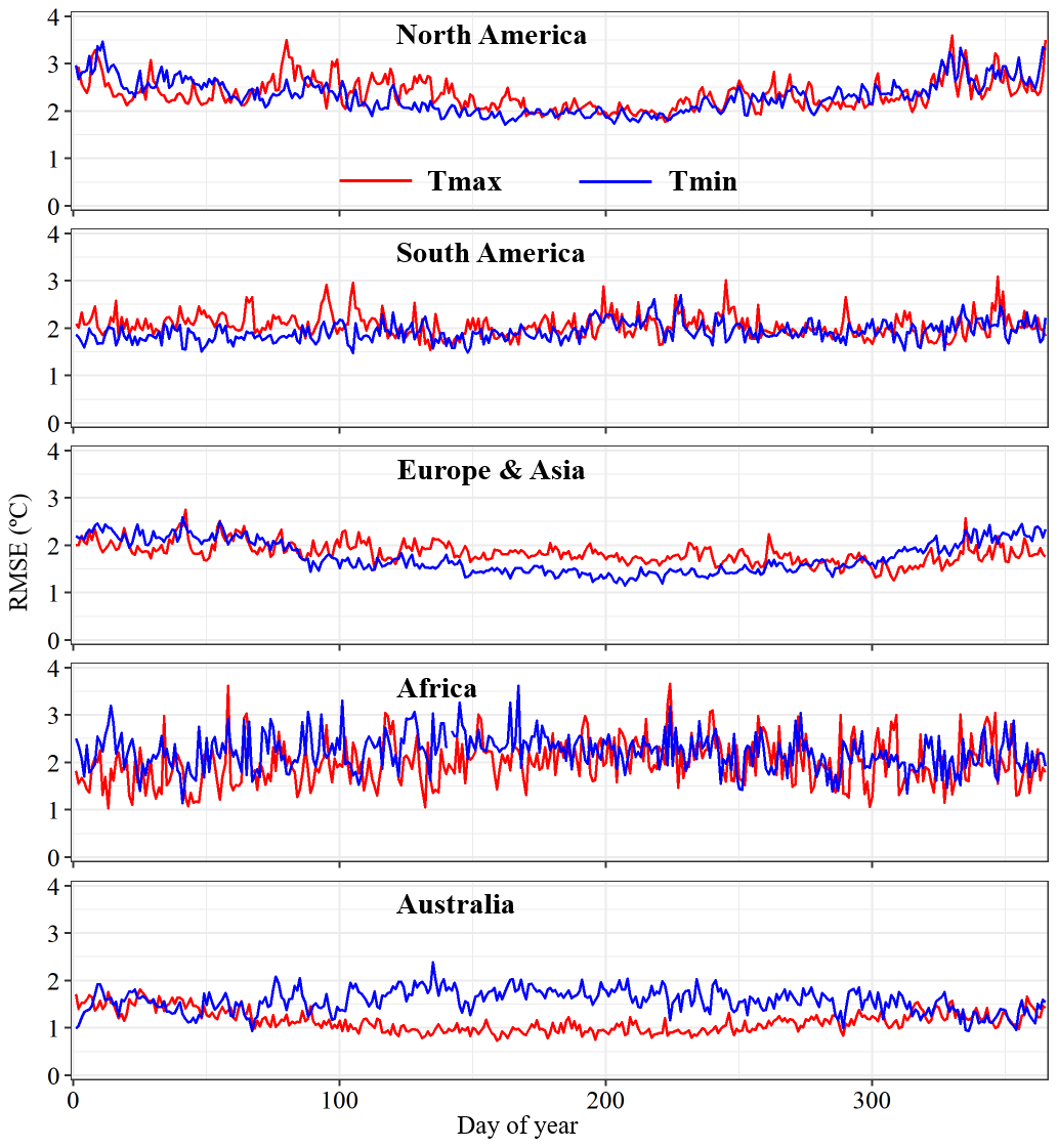
Figure 5Temporal patterns of accuracies in estimated Ta in different regions in the year 2010.
The RMSE values generally show distinctly seasonal patterns in the five regions within reasonable ranges (Fig. 5). Taking the year 2010 as an example, RMSEs in summer (June, July, and August) are generally lower than those in winter (December, January, and February) in North American, European, and Asian regions (Fig. 5) possibly due to plant phenology, which leads to a closer relationship between Ta and LST in the summer than in the winter (Benali et al., 2012; Cai et al., 2017; Lin et al., 2012). This seasonal variation is less obvious in Africa and South America possibly due to weaker correlations between plant phenology and air temperature in the two regions, which are located across the Equator (Adole et al., 2019; Sakai and Kitajima, 2019). Specifically, the Australian region, which is located in the Southern Hemisphere, shows higher RMSEs in summer (December, January, and February) than in winter (June, July, and August) for Tmax. This may be caused by more homogeneous spatial variations in Tmax in winter than in summer in the Australian region.
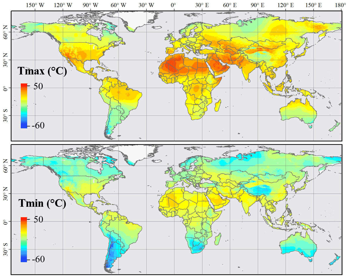
Figure 6Spatial pattern of estimated Ta at the global scale on an example day, day 200, in 2010.
4.2 Spatial and temporal patterns of Ta
The estimated Ta shows significant spatial variations at the global scale (Fig. 6). Taking the estimated Ta on one July day as an example, both Tmax and Tmin decrease from about 30∘ N to the North and South poles (Fig. 6). Meanwhile, lower Ta values also occur at higher-elevation regions such as the Tibetan Plateau in the center of Asia and the Andes Mountains in the west of South America. Therefore, the characteristics of Ta change with latitude and elevation (i.e., the trend of lower Ta in higher-latitude/elevation areas), which is consistent with the existing studies (Chen et al., 2015; Zhang et al., 2022b). The highest Ta values occur in northern Africa and the Arabian Peninsula, as these regions are mainly covered by the Gobi Desert.
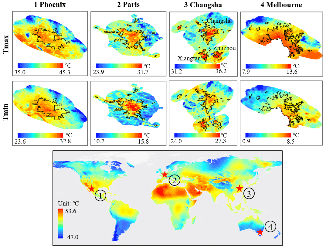
Figure 7Spatial pattern of estimated Ta in five representative cities on day 200 of the year 2010. A city shape includes the urban Ta extracted by using nighttime light data (Zhou et al., 2018) and a surrounding buffer of equal size. Black polygons are the urban extents extracted by using global 30 m resolution artificial impervious area data (Li et al., 2020).
The spatial patterns of estimated Ta in selected cities with clear weather around the world illustrate that the urban heat island (UHI) phenomenon (i.e., the higher temperature in urban than in the surrounding rural areas) has been well captured at the city scale (Fig. 7). On an example day of July in 2010, the estimated Ta in these cities shows an obvious UHI phenomenon, which is reasonable with the transition from urban centers to surrounding rural areas. The estimated Ta in Changsha, China, shows several hotspots because some nearby cities (such as Xiangtan and Zhuzhou) have also been included in the buffer of Changsha, indicating the effectiveness of the estimated Ta for presenting UHI in small urban areas. Specifically, as a coastal city, estimated Ta in Melbourne, Australia, shows decreasing trends from the coast, and the UHI phenomenon is not obvious in surrounding small cities. This is because there is also an increasing trend of elevation from the coast in Melbourne, leading to the mixed spatial patterns of Ta due to the UHI phenomenon and elevation changes.
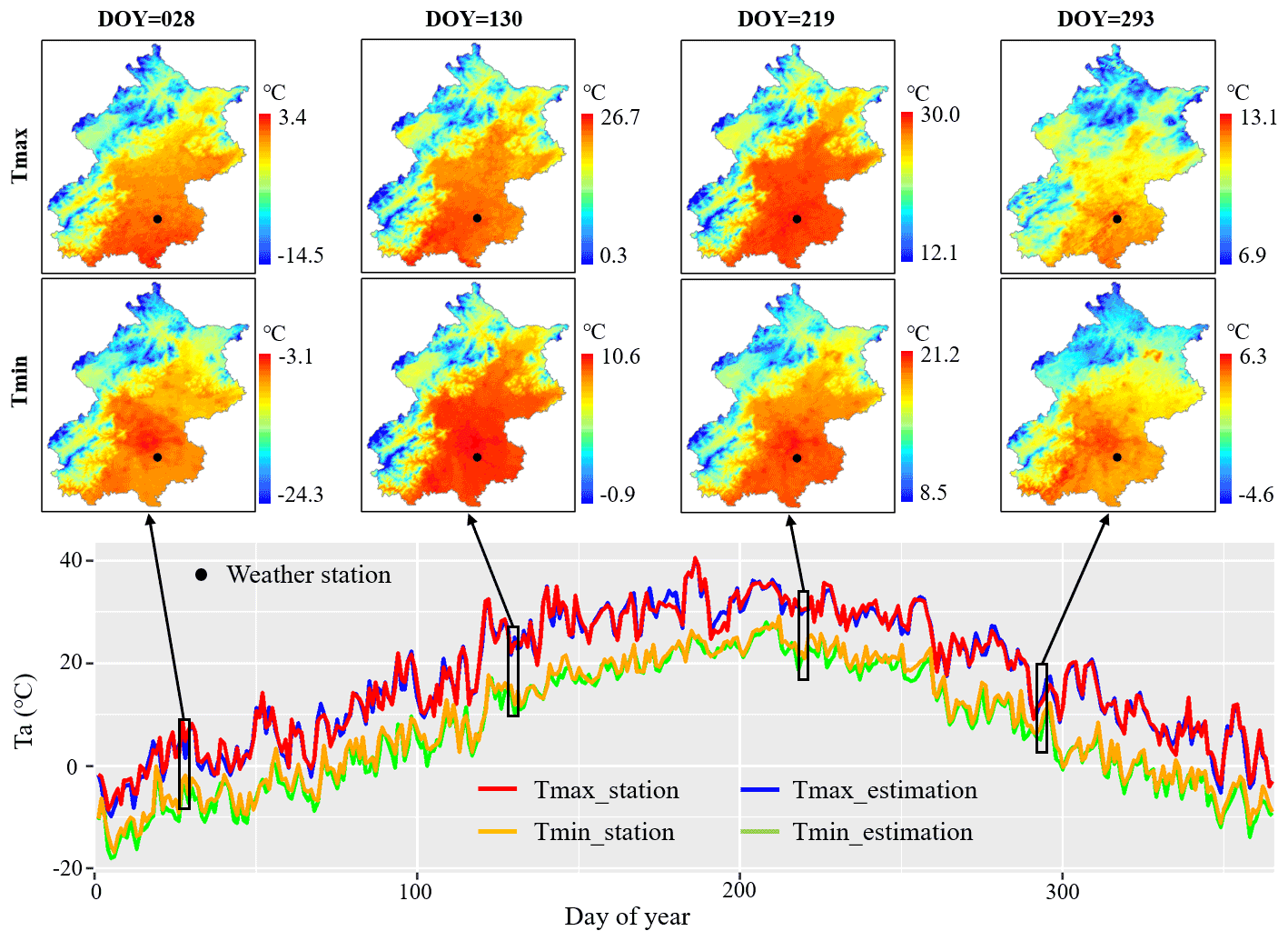
Figure 8Temporal pattern of estimated and observed Ta at the weather station of Beijing (black point) in the year 2010. The black rectangles are example days showing maps of estimated data in Beijing.
The comparison of the temporal pattern between estimated Ta and ground-station-based measurements from an example of weather stations in a mega-city (Fig. 8) illustrates that the SVCM-SP algorithm can effectively (RMSE of 1.25 ∘C and 1.53 ∘C, respectively, for Tmax and Tmin) estimate Ta for the entire period. As shown in Fig. 8, the estimated Ta based on 10-fold cross-validation and Ta observations from the weather station in Beijing, China, show similar temporal patterns and very close values for both Tmax and Tmin in 2010. For both clear weather (days 28 and 130 in Fig. 8) and overcast weather (days 219 and 293 in Fig. 8) (Zhang et al., 2022a), the gridded Ta can illustrate the UHI phenomenon. An existing study has found that the estimated Ta in urban areas was more accurate than those of other regions (Zhang et al., 2022b), specifically suggesting its great value for urban applications.
4.3 Comparison with existing Ta datasets
The gridded Ta data in this study have advantages regarding spatiotemporal resolutions (i.e., 1 km and daily maximum and minimum) and its global coverage (Table S3). The spatial resolution of existing global Ta datasets with daily frequencies and long-term coverage is generally low (e.g., 0.25∘) (Hersbach et al., 2018; Kalnay et al., 1996). Ta datasets with improved spatial resolutions (e.g., 1 km) are usually only available at the continental or national scales (Chen et al., 2021; Fang et al., 2021; MacDonald et al., 2020; Oyler et al., 2015; Thornton et al., 2021).
The gridded Ta in this study can effectively capture the spatial variation in Ta by preserving physical relationships between Ta and response variables (Fig. S7 in the Supplement). In other Ta datasets, such physical relationships (e.g., positive relationship between Ta and LST) cannot always be preserved in some situations because these datasets were created using methods without explicit constraints on the relationships between Ta and response variables. Efforts have been made to build vertical lapse models to estimate gridded Ta according to adiabatic lapse rate (ALR) (Dodson and Marks, 1997; Rhee and Im, 2014; Thornton et al., 2021; Zhu et al., 2017), but the generalization of these models is limited because it is difficult to accurately capture ALR due to its spatial change.
The accuracy of the resulting gridded Ta from this study is comparable to several other reported gridded Ta datasets (e.g., Chen et al., 2021; Oyler et al., 2015; Thornton et al., 2021). Among them, the 1 km daily Ta from Daymet (Thornton et al., 2021) reaches an MAE of 1.52 and 1.78 ∘C for Tmax and Tmin, respectively, and the 30 arcsec (∼ 800 m) daily Ta from TopoWx (Oyler et al., 2015) reaches 1.03 and 1.06 ∘C, while in this study, the average MAE is 1.82 and 1.78 ∘C in North America. However, Daymet failed to capture the UHI phenomenon due to the spatial interpolation of Ta being implemented based only on elevation (Menne et al., 2012) and did not consider the impact of biophysical and socioeconomic factors on spatial variations in Ta (Li et al., 2018). Therefore, Daymet has difficulties in capturing the spatial variation in Ta in urban areas, although its accuracy is comparable to our dataset. The estimated Ta from TopoWx can display the UHI phenomenon but tends to overestimate the impact of topographical features and show fewer temporal variations in the spatial pattern of Ta within a month than that in this study, as a 10-year average of monthly LSTs was used as a covariate in TopoWx (Li et al., 2018; Oyler et al., 2015) instead of daily LST data in this study. The 1 km daily average Ta data by Chen et al. (2021) reach a RMSE of 1.615 to 1.957 K using leave-location-out cross-validation in mainland China, while the average RMSE of estimated Tmax and Tmin is 1.80 and 1.75 ∘C, respectively, in Europe and Asia. While the accuracy of Ta obtained in this study is comparable to the other large-scale Ta datasets, our dataset is produced at the global scale using consistent modeling and assessment approaches.
There are some limitations in the SVCM-SP algorithm used in this study for creating the gridded Ta dataset, and future work can focus on improving the accuracy of the estimated Ta with an improved SVCM-SP algorithm. First, we only considered the linear relationship between Ta and covariates. However, nonlinear relationships may exist between Ta with elevation and LST when other factors, such as winds, clouds, snow, and land cover types, have non-negligible impacts on Ta (Cai et al., 2017; Good, 2016). Second, we only used two covariates in the SVCM-SP algorithm, although the potential of generalization of our framework is large. Additional covariates (e.g., other surface characters such as Geoscience Laser Altimeter System (GLAS)-derived canopy height and vegetation parameters) can be explored in the SVCM-SP algorithm to further improve the model performance. Third, the limited number of valid station observations on specific days might introduce larger uncertainties in interpolating Ta using the SVCM-SP algorithm. In future studies, station observations from neighboring days can be explored to improve the interpolation of Ta.
Data described in this paper can be accessed at Iowa State University's DataShare at https://doi.org/10.25380/iastate.c.6005185 (Zhang and Zhou, 2022). The dataset contains 36 sub-datasets. Each sub-dataset contains Tmax or Tmin of each year from 2003 to 2020 in five regions (i.e., North America, South America, Europe and Asia, Africa, and Australia and New Zealand). The data are in GeoTIFF with the georeferenced information embedded. The MODIS ellipse sinusoidal projection with a spatial resolution of 1 km is used in the data. The unit of LST in GeoTIFF is 0.1∘ Celsius (∘C), and the naming rule can be found in the file “README.pdf”.
We generated a global land (50∘ S–79∘ N) 1 km daily maximum and minimum Ta (i.e., Tmax and Tmin) dataset from 2003 to 2020 based on ground-station-based Ta measurements and gap-filled LST dataset using the Spatially Varying Coefficient Models with Sign Preservation (SVCM-SP) algorithm. The dataset showed acceptable accuracies based on the 10-fold cross-validation for five regions of the globe compared to existing Ta datasets. The RMSEs of estimated Tmax and Tmin ranged from 1.20 to 2.44 and 1.69 to 2.39 ∘C, respectively. The estimated Ta was affected by land cover types, elevation ranges, and climate types, with varying accuracies but within reasonable ranges. Our gridded Ta dataset effectively captured the spatial variation in Ta under clear physical meanings (i.e., negative and positive relationships with elevation and LST, respectively), which is not always true in other gridded Ta datasets. The new dataset is unique in terms of spatiotemporal resolutions (i.e., 1 km daily maximum and minimum), global coverage, and temporal span and should be useful for a wide range of applications such as the urban heat island phenomenon, hydrological modeling, and epidemic forecasting. Future work can focus on improving the accuracy of the gridded Ta dataset using the SVCM-SP algorithm by exploring more explanatory variables which are available over large areas.
The supplement related to this article is available online at: https://doi.org/10.5194/essd-14-5637-2022-supplement.
YZ designed the research, TZ implemented the research and wrote the original manuscript, and YZ and ZZ supervised the research. All co-authors revised the manuscript and contributed to the writing.
At least one of the (co-)authors is a member of the editorial board of Earth System Science Data. The peer-review process was guided by an independent editor, and the authors also have no other competing interests to declare.
Publisher's note: Copernicus Publications remains neutral with regard to jurisdictional claims in published maps and institutional affiliations.
This research was supported by the College of Liberal Arts and Science (LAS) Dean's Emerging Faculty Leaders award at the Iowa State University and the National Science Foundation (2041859, 1803920, and 2203207).
This paper was edited by Jing Wei and reviewed by three anonymous referees.
Adole, T., Dash, J., Rodriguez-Galiano, V., and Atkinson, P. M.: Photoperiod controls vegetation phenology across Africa, Commun. Biol., 2, 1–13, https://doi.org/10.1038/s42003-019-0636-7, 2019.
Becker, J. J., Sandwell, D. T., Smith, W. H. F., Braud, J., Binder, B., Depner, J., Fabre, D., Factor, J., Ingalls, S., Kim, S. H., Ladner, R., Marks, K., Nelson, S., Pharaoh, A., Trimmer, R., von Rosenberg, J., Wallace, G., and Weatherall, P.: Global Bathymetry and Elevation Data at 30 Arc Seconds Resolution: SRTM30_PLUS, Mar. Geod., 32, 355–371, https://doi.org/10.1080/01490410903297766, 2009.
Benali, A., Carvalho, A. C., Nunes, J. P., Carvalhais, N., and Santos, A.: Estimating air surface temperature in Portugal using MODIS LST data, Remote Sens. Environ., 124, 108–121, https://doi.org/10.1016/j.rse.2012.04.024, 2012.
Cai, Y., Chen, G., Wang, Y., and Yang, L.: Impacts of land cover and seasonal variation on maximum air temperature estimation using MODIS imagery, Remote Sens.-Basel, 9, 3, https://doi.org/10.3390/rs9030233, 2017.
Chai, H., Cheng, W., Zhou, C., Chen, X., Ma, X., and Zhao, S.: Analysis and comparison of spatial interpolation methods for temperature data in Xinjiang Uygur Autonomous Region, China, Nat. Sci., 03, 999–1010, https://doi.org/10.4236/ns.2011.312125, 2011.
Chen, F., Liu, Y., Liu, Q., and Qin, F.: A statistical method based on remote sensing for the estimation of air temperature in China, Int. J. Climatol., 35, 2131–2143, https://doi.org/10.1002/joc.4113, 2015.
Chen, Y., Liang, S., Ma, H., Li, B., He, T., and Wang, Q.: An all-sky 1 km daily land surface air temperature product over mainland China for 2003–2019 from MODIS and ancillary data, Earth Syst. Sci. Data, 13, 4241–4261, https://doi.org/10.5194/essd-13-4241-2021, 2021.
Connor, S. J., Flasse, S. P., Thomson, M. C., and Perryman, A. H.: Environmental information systems in malaria risk mapping and epidemic forecasting, Disasters, 22, 39–56, https://doi.org/10.1111/1467-7717.00074, 1998.
Crespi, A., Matiu, M., Bertoldi, G., Petitta, M., and Zebisch, M.: A high-resolution gridded dataset of daily temperature and precipitation records (1980–2018) for Trentino-South Tyrol (north-eastern Italian Alps), Earth Syst. Sci. Data, 13, 2801–2818, https://doi.org/10.5194/essd-13-2801-2021, 2021.
Danielson, J. J. and Gesch, D. B.: Global multi-resolution terrain elevation data 2010 (GMTED2010), Washington, DC, USA, US Department of the Interior, US Geological Survey, https://pubs.usgs.gov/of/2011/1073/pdf/of2011-1073.pdf (last access: 15 December 2022), 2011.
Dimarzio, J., Brenner, A., Fricker, H., Schutz, R., Shuman, C., and Zwally, H.: GLAS/ICESat 500 m laser altimetry digital elevation model of Antarctica, Version 1, [online] https://nsidc.org/data/NSIDC-0304/versions/1 (last access: 18 May 2021), 2007.
Dodson, R. and Marks, D.: Daily air temperature interpolated at high spatial resolution over a large mountainous region, Clim. Res., 8, 1–20, https://doi.org/10.3354/cr008001, 1997.
Fang, S., Mao, K., Xia, X., Wang, P., Shi, J., Bateni, S. M., Xu, T., Cao, M., Heggy, E., and Qin, Z.: Dataset of daily near-surface air temperature in China from 1979 to 2018, Earth Syst. Sci. Data, 14, 1413–1432, https://doi.org/10.5194/essd-14-1413-2022, 2022.
Good, E. J.: An in situ-based analysis of the relationship between land surface “skin” and screen-level air temperatures, J. Geophys. Res.-Atmos., 121, 8801–8819, https://doi.org/10.1002/2016JD025318, 2016.
Goward, S. N., Waring, R. H., Dye, D. G., and Yang, J.: Ecological Remote Sensing at OTTER: Satellite Macroscale Observations, Ecol. Appl., 4, 322–343, 1994.
Hengl, T., Heuvelink, G. B. M., Tadić, M. P., and Pebesma, E. J.: Spatio-temporal prediction of daily temperatures using time-series of MODIS LST images, Theor. Appl. Climatol., 107, 265–277, https://doi.org/10.1007/s00704-011-0464-2, 2012.
Hennig, T. A., Kretsch, J. L., Pessagno, C. J., Salamonowicz, P. H., and Stein, W. L.: The shuttle radar topography mission, in: Digital Earth Moving, edited by: Westort, C. Y., Lect. Notes Comput. Sci. (including Sub-ser. Lect. Notes Artif. Intell. Lect. Notes Bioinformatics), 2181, 65–77, https://doi.org/10.1007/3-540-44818-7_11, 2001.
Hersbach, H., Bell, B., Berrisford, P., Biavati, G., Horányi, A., Muñoz Sabater, J., Nicolas, J., Peubey, C., Radu, R., and Rozum, I.: ERA5 hourly data on single levels from 1979 to present, Copernicus Climate Change Service (C3S) Climate Data Store (CDS), ECMWF, 147, 5–6, 2018.
Hooker, J., Duveiller, G., and Cescatti, A.: Data descriptor: A global dataset of air temperature derived from satellite remote sensing and weather stations, Sci. Data, 5, 1–11, https://doi.org/10.1038/sdata.2018.246, 2018.
Hou, P., Chen, Y., Qiao, W., Cao, G., Jiang, W., and Li, J.: Near-surface air temperature retrieval from satellite images and influence by wetlands in urban region, Theor. Appl. Climatol., 111, 109–118, https://doi.org/10.1007/s00704-012-0629-7, 2013.
Hrisko, J., Ramamurthy, P., Yu, Y., Yu, P., and Melecio-Vázquez, D.: Urban air temperature model using GOES-16 LST and a diurnal regressive neural network algorithm, Remote Sens. Environ., 237, 111495, https://doi.org/10.1016/j.rse.2019.111495, 2020.
Huang, M., Piao, S., Ciais, P., Peñuelas, J., Wang, X., Keenan, T. F., Peng, S., Berry, J. A., Wang, K., Mao, J., Alkama, R., Cescatti, A., Cuntz, M., De Deurwaerder, H., Gao, M., He, Y., Liu, Y., Luo, Y., Myneni, R. B., Niu, S., Shi, X., Yuan, W., Verbeeck, H., Wang, T., Wu, J., and Janssens, I. A.: Air temperature optima of vegetation productivity across global biomes, Nat. Ecol. Evol., 3, 772–779, https://doi.org/10.1038/s41559-019-0838-x, 2019.
Kalnay, E., Kanamitsu, M., Kistler, R., Collins, W., Deaven, D., Gandin, L., Iredell, M., Saha, S., White, G., Woollen, J., Zhu, Y., Chelliah, M., Ebisuzaki, W., Higgins, W., Janowiak, J., Mo, K. C., Ropelewski, C., Wang, J., Leetmaa, A., Reynolds, R., Jenne, R., and Joseph, D.: The NCEP/NCAR 40-year reanalysis project, B. Am. Meteorol. Soc., 77, 437–472, https://doi.org/10.1175/1520-0477(1996)077<0437:TNYRP>2.0.CO;2, 1996.
Kim, M., Wang, L., and Zhou, Y.: Spatially varying coefficient models with sign preservation of the coefficient functions, J. Agr. Biol. Envir. St., 26, 367–386, https://doi.org/10.1007/s13253-021-00443-5, 2021.
Lan, L., Lian, Z., and Pan, L.: The effects of air temperature on office workers' well-being, workload and productivity-evaluated with subjective ratings, Appl. Ergon., 42, 29–36, https://doi.org/10.1016/j.apergo.2010.04.003, 2010.
Lan, L., Tang, J., Wargocki, P., Wyon, D. P., and Lian, Z.: Cognitive performance was reduced by higher air temperature even when thermal comfort was maintained over the 24–28 ∘C range, Indoor Air, 32, 1–15, https://doi.org/10.1111/ina.12916, 2022.
Legates, D. R. and Willmott, C. J.: Mean seasonal and spatial variability in global surface air temperature, Theor. Appl. Climatol., 41, 11–21, https://doi.org/10.1007/BF00866198, 1990.
Li, J. and Heap, A. D.: A review of comparative studies of spatial interpolation methods in environmental sciences: Performance and impact factors, Ecol. Inform., 6, 228–241, https://doi.org/10.1016/j.ecoinf.2010.12.003, 2011.
Li, L. and Zha, Y.: Estimating monthly average temperature by remote sensing in China, Adv. Space Res., 63, 2345–2357, https://doi.org/10.1016/j.asr.2018.12.039, 2019.
Li, X., Zhou, Y., Asrar, G. R., and Zhu, Z.: Developing a 1 km resolution daily air temperature dataset for urban and surrounding areas in the conterminous United States, Remote Sens. Environ., 215, 74–84, https://doi.org/10.1016/j.rse.2018.05.034, 2018.
Li, X., Gong, P., Zhou, Y., Wang, J., Bai, Y., Chen, B., Hu, T., Xiao, Y., Xu, B., Yang, J., Liu, X., Cai, W., Huang, H., Wu, T., Wang, X., Lin, P., Li, X., Chen, J., He, C., Li, X., Yu, L., Clinton, N., and Zhu, Z.: Mapping global urban boundaries from the global artificial impervious area (GAIA) data, Environ. Res. Lett., 15, 094044, https://doi.org/10.1088/1748-9326/ab9be3, 2020.
Lin, S., Moore, N. J., Messina, J. P., DeVisser, M. H., and Wu, J.: Evaluation of estimating daily maximum and minimum air temperature with MODIS data in east Africa, Int. J. Appl. Earth Obs., 18, 128–140, https://doi.org/10.1016/j.jag.2012.01.004, 2012.
Lowen, A. C., Mubareka, S., Steel, J., and Palese, P.: Influenza virus transmission is dependent on relative humidity and temperature, PLoS Pathog., 3, 1470–1476, https://doi.org/10.1371/journal.ppat.0030151, 2007.
MacDonald, H., McKenney, D. W., Papadopol, P., Lawrence, K., Pedlar, J., and Hutchinson, M. F.: North American historical monthly spatial climate dataset, 1901–2016, Sci. Data, 7, 1–11, https://doi.org/10.1038/s41597-020-00737-2, 2020.
Menne, M. J., Durre, I., Vose, R. S., Gleason, B. E., and Houston, T. G.: An overview of the global historical climatology network-daily database, J. Atmos. Ocean. Tech., 29, 897–910, https://doi.org/10.1175/JTECH-D-11-00103.1, 2012.
Meyer, H., Schmidt, J., Detsch, F., and Nauss, T.: Hourly gridded air temperatures of South Africa derived from MSG SEVIRI, Int. J. Appl. Earth Obs., 78, 261–267, https://doi.org/10.1016/j.jag.2019.02.006, 2019.
Nashwan, M. S., Shahid, S., and Chung, E. S.: Development of high-resolution daily gridded temperature datasets for the central north region of Egypt, Sci. Data, 6, 1–13, https://doi.org/10.1038/s41597-019-0144-0, 2019.
Nemani, R. R. and Running, S. W.: Estimation of Regional Surface Resistance to Evapotranspiration from NDVI and Thermal-IR AVHRR Data, J. Appl. Meteorol. Clim., 28, 276–284, https://doi.org/10.1175/1520-0450(1989)028{%}3C0276:EORSRT{%}3E2.0.CO;2, 1989.
Noi, P. T., Degener, J., and Kappas, M.: Comparison of multiple linear regression, cubist regression, and random forest algorithms to estimate daily air surface temperature from dynamic combinations of MODIS LST data, Remote Sens.-Basel, 9, 398, https://doi.org/10.3390/rs9050398, 2017.
Oyler, J. W., Ballantyne, A., Jencso, K., Sweet, M., and Running, S. W.: Creating a topoclimatic daily air temperature dataset for the conterminous United States using homogenized station data and remotely sensed land skin temperature, Int. J. Climatol., 35, 2258–2279, https://doi.org/10.1002/joc.4127, 2015.
Petrova, V. N. and Russell, C. A.: The evolution of seasonal influenza viruses, Nat. Rev. Microbiol., 16, 47–60, https://doi.org/10.1038/nrmicro.2017.118, 2018.
Prihodko, L. and Goward, S. N.: Estimation of air temperature from remotely sensed surface observations, Remote Sens. Environ., 60, 335–346, https://doi.org/10.1016/S0034-4257(96)00216-7, 1997.
Rao, Y., Liang, S., Wang, D., Yu, Y., Song, Z., Zhou, Y., Shen, M., and Xu, B.: Estimating daily average surface air temperature using satellite land surface temperature and top-of-atmosphere radiation products over the Tibetan Plateau, Remote Sens. Environ., 234, 111462, https://doi.org/10.1016/j.rse.2019.111462, 2019.
Ren, S., Qin, Q., and Ren, H.: Contrasting wheat phenological responses to climate change in global scale, Sci. Total Environ., 665, 620–631, https://doi.org/10.1016/j.scitotenv.2019.01.394, 2019.
Rhee, J. and Im, J.: Estimating high spatial resolution air temperature for regions with limited in situ data using MODIS products, Remote Sens.-Basel, 6, 7360–7378, https://doi.org/10.3390/rs6087360, 2014.
Rosen, P. A.: Synthetic aperture radar interferometry, P. IEEE, 88, 333–380, https://doi.org/10.1109/5.838084, 2000.
Sakai, S. and Kitajima, K.: Tropical phenology: Recent advances and perspectives, Ecol. Res., 34, 50–54, https://doi.org/10.1111/1440-1703.1131, 2019.
Shen, H., Jiang, Y., Li, T., Cheng, Q., Zeng, C., and Zhang, L.: Deep learning-based air temperature mapping by fusing remote sensing, station, simulation and socioeconomic data, Remote Sens. Environ., 240, 111692, https://doi.org/10.1016/j.rse.2020.111692, 2020.
Shi, Y., Jiang, Z., Dong, L., and Shen, S.: Statistical estimation of high-resolution surface air temperature from MODIS over the Yangtze River Delta, China, J. Meteorol. Res.-PRC, 31, 448–454, https://doi.org/10.1007/s13351-017-6073-y, 2017.
Stahl, K., Moore, R. D., Floyer, J. A., Asplin, M. G., and McKendry, I. G.: Comparison of approaches for spatial interpolation of daily air temperature in a large region with complex topography and highly variable station density, Agr. Forest Meteorol., 139, 224–236, https://doi.org/10.1016/j.agrformet.2006.07.004, 2006.
Sulla-Menashe, D. and Friedl, M. A.: User Guide to Collection 6 MODIS Land Cover Dynamics (MCD12Q2) Product, User Guid., 6, 1–18, https://modis-land.gsfc.nasa.gov/pdf/MCD12Q1_C6_Userguide04042018.pdf (last access: 15 December 2022), 2018.
Sun, Y. J., Wang, J. F., Zhang, R. H., Gillies, R. R., Xue, Y., and Bo, Y. C.: Air temperature retrieval from remote sensing data based on thermodynamics, Theor. Appl. Climatol., 80, 37–48, https://doi.org/10.1007/s00704-004-0079-y, 2005.
Thornton, P. E., Shrestha, R., Thornton, M., Kao, S. C., Wei, Y., and Wilson, B. E.: Gridded daily weather data for North America with comprehensive uncertainty quantification, Sci. Data, 8, 1–17, https://doi.org/10.1038/s41597-021-00973-0, 2021.
Verma, P., Sarkar, S., Singh, P., and Dhiman, R. C.: Devising a method towards development of early warning tool for detection of malaria outbreak, The Indian Journal of Medical Research, 146, 612–621, https://www.ncbi.nlm.nih.gov/pmc/articles/PMC5861472/ (last access: 15 December 2022), 2017.
Werner, A. T., Schnorbus, M. A., Shrestha, R. R., Cannon, A. J., Zwiers, F. W., Dayon, G., and Anslow, F.: A long-term, temporally consistent, gridded daily meteorological dataset for northwestern North America, Sci. Data, 6, 1–16, https://doi.org/10.1038/sdata.2018.299, 2019.
Wu, Y., Jing, W., Liu, J., Ma, Q., Yuan, J., Wang, Y., Du, M., and Liu, M.: Effects of temperature and humidity on the daily new cases and new deaths of COVID-19 in 166 countries, Sci. Total Environ., 729, 1–7, https://doi.org/10.1016/j.scitotenv.2020.139051, 2020.
Yoo, C., Im, J., Park, S., and Quackenbush, L. J.: Estimation of daily maximum and minimum air temperatures in urban landscapes using MODIS time series satellite data, ISPRS J. Photogramm., 137, 149–162, https://doi.org/10.1016/j.isprsjprs.2018.01.018, 2018.
Zhang, F., de Dear, R., and Hancock, P.: Effects of moderate thermal environments on cognitive performance: A multidisciplinary review, Appl. Energ., 236, 760–777, https://doi.org/10.1016/j.apenergy.2018.12.005, 2019.
Zhang, R., Rong, Y., Tian, J., Su, H., Li, Z. L., and Liu, S.: A remote sensing method for estimating surface air temperature and surface vapor pressure on a regional Scale, Remote Sens.-Basel, 7, 6005–6025, https://doi.org/10.3390/rs70506005, 2015.
Zhang, T. and Zhou, Y.: A global 1 km resolution daily near-surface air temperature dataset (2003–2020), Iowa State University [data set], https://doi.org/10.25380/iastate.c.6005185, 2022.
Zhang, T., Zhou, Y., Zhu, Z., Li, X., and Asrar, G. R.: A global seamless 1 km resolution daily land surface temperature dataset (2003–2020), Earth Syst. Sci. Data, 14, 651–664, https://doi.org/10.5194/essd-14-651-2022, 2022a.
Zhang, T., Zhou, Y., Wang, L., Zhao, K., and Zhu, Z.: Estimating 1 km gridded daily air temperature using a spatially varying coefficient model with sign preservation, Remote Sens. Environ., 277, 113072, https://doi.org/10.1016/j.rse.2022.113072, 2022b.
Zhang, Z., Chang, J., Xu, C. Y., Zhou, Y., Wu, Y., Chen, X., Jiang, S., and Duan, Z.: The response of lake area and vegetation cover variations to climate change over the Qinghai-Tibetan Plateau during the past 30 years, Sci. Total Environ., 635, 443–451, https://doi.org/10.1016/j.scitotenv.2018.04.113, 2018.
Zhou, Y., Li, X., Asrar, G. R., Smith, S. J., and Imhoff, M.: A global record of annual urban dynamics (1992–2013) from nighttime lights, Remote Sens. Environ., 219, 206–220, https://doi.org/10.1016/j.rse.2018.10.015, 2018.
Zhu, W., Lu, A., and Jia, S.: Estimation of daily maximum and minimum air temperature using MODIS land surface temperature products, Remote Sens. Environ., 130, 62–73, https://doi.org/10.1016/j.rse.2012.10.034, 2013.
Zhu, W., Lű, A., Jia, S., Yan, J., and Mahmood, R.: Retrievals of all-weather daytime air temperature from MODIS products, Remote Sens. Environ., 189, 152–163, https://doi.org/10.1016/j.rse.2016.11.011, 2017.