Location, biophysical and agronomic parameters for croplands in northern Ghana

Smallholder agriculture is the bedrock of the food production system in sub-Saharan Africa. Yields in Africa are significantly below potentially attainable yields for a number of reasons, and they are particularly vulnerable to climate change impacts. Monitoring of these highly heterogeneous landscapes is needed to respond to farmer needs, develop an appropriate policy and ensure food security, and Earth observation (EO) must be part of these efforts, but there is a lack of ground data for developing and testing EO methods in western Africa, and in this paper, we present data on (i) crop locations, (ii) biophysical parameters and (iii) crop yield, and biomass was collected in 2020 and 2021 in Ghana and is reported in this paper. In 2020, crop type was surveyed in more than 1800 fields in three different agroecological zones across Ghana (the Guinea Savannah, Transition and Deciduous zones). In 2021, a smaller number of fields were surveyed in the Guinea Savannah zone, and additionally, repeated measurements of leaf area index (LAI) and leaf chlorophyll concentration were made on a set of 56 maize fields. Yield and biomass were also sampled at harvesting. LAI in the sampled fields ranged from 0.1 to 5.24 m² m⁻², whereas leaf chlorophyll concentration varied between 6.1 and 60.3 µg cm⁻². Yield varied between 190 and 4580 kg ha⁻¹, with an important within-field variability (average per-field standard deviation 381 kg ha⁻¹). The data are used in this paper to (i) evaluate the Digital Earth Africa 2019 cropland masks, where 61 % of sampled 2020/21 cropland is flagged as cropland by the data set, (ii) develop and test an LAI retrieval method from Earth observation Planet surface reflectance data (validation correlation coefficient R=0.49, root mean square error (RMSE) 0.44 m² m⁻²), (iii) create a maize classification data set for Ghana for 2021 (overall accuracy within the region tested: 0.84), and (iv) explore the relationship between maximum LAI and crop yield using a linear model (correlation coefficient R=0.66 and R=0.53 for in situ and Planet-derived LAI, respectively). The data set, made available here within the context of the Group on Earth Observations Global Agricultural Monitoring (GEOGLAM) initiative, is an important contribution to understanding crop evolution and distribution in smallholder farming systems and will be useful for researchers developing/validating methods to monitor these systems using Earth observation data. The data described in this paper are available from https://doi.org/10.5281/zenodo.6632083 (Gomez-Dans et al., 2022).

1 Introduction

Agricultural production in sub-Saharan Africa is dominated by smallholder farms that support most households (Giller et al., 2021; Antonaci et al., 2014). In Ghana, agriculture contributes around 20 % of gross domestic product (GDP) and employs around half of the population (SRID, 2010). Maize accounts for more than half of the country's cereal production (Ragasa et al., 2014), and in the north of the country, the crop is grown in rain-fed conditions, with low inputs (limited use of fertiliser, low uptake of modern/hybrid varieties, low mechanisation) suffering additionally from considerable post-harvesting losses and nutrient-poor soils (Freduah et al., 2019; MacCarthy et al., 2017; Sánchez, 2010; SRID, 2010). These factors result in an important yield gap compared to potential attainable yields (van Loon et al., 2019; Cairns et al., 2013). This yield gap is exacerbated in a climate change context, where agricultural production in Ghana is likely to be further limited by increased temperature and more erratic rain regimes (Sultan and Gaetani, 2016; Chemura et al., 2020), with complex relationships with nitrogen use (Falconnier et al., 2020) and other social factors (Nyantakyi-Frimpong and Bezner-Kerr, 2015) adding further vulnerability to yields in the region.

Timely monitoring of smallholder maize production is important for understanding the developing food security situation but also for providing information to food producers and other value creators. Decision-makers at regional or national levels need this for planning policy, import–export requirements or other advance planning or support mechanisms for farmers (Nations, 2013; Nakalembe et al., 2021). Monitoring capabilities are also important for developing crop insurance and maximising the economic potential (and hence livelihoods) of smallholder farmers (Benami et al., 2021). At more local scales, such information can be used by extension workers to assist farmers in improving their practice. Carletto et al. (2013) argue that a lack of good-quality agricultural data in Africa has hampered innovation and growth in this crucial economic sector.

In Ghana, 60 % of farms have an area of less than 1.2 ha (SRID, 2010), giving rise to a highly heterogeneous landscape. Some factors that explain this heterogeneity are also common with the yield gap: limited access to e.g. irrigation, mechanisation and fertiliser use, workforce scarcity, low labour productivity, or limited access to finance (van Loon et al., 2019). Local patterns of crop yield are known to be impacted by local soil and meteorological conditions as well as farmer choices. For example, Freduah et al. (2019) note that maize planting occurs over a 3-month period, with further crop development variation depending on the use of fertiliser and other management practices. This, alongside the varying quality of seed inputs, results in very different inter- and intra-field crop evolution even for crops subject to very similar weather patterns. This complicates both monitoring and modelling efforts.

There is a strong need for better information on cropland area, crop productivity and the factors that affect crop production in Africa. Earth observation (EO) has been shown to provide a practical data source for monitoring croplands over large areas for much of the world and contributing to the collection of better agronomic statistics. This in turn can be used by decision-makers, agronomists and other parties to better understand and plan actions to improve food security and alleviating poverty (e.g. Baruth et al., 2008; Carletto et al., 2015; Brown, 2016).

To monitor agriculture, the first layer of information maps the areas of croplands to distinguish them from other land uses, but even this basic information is currently very uncertain for large parts of Ghana. To be able to estimate total production or even average productivity in some region, an additional level of sophistication is needed on top of that where the crop type is identified. While there have been some recent advances in cropland masks derived from Earth observation for the region (Burton et al., 2022; Estes et al., 2022; Xiong et al., 2017), accurate, timely data sets that allow the location of individual crops over large areas are still mainly lacking.

The advent of frequent, medium- to high-resolution EO data over the last ∼5 years from sensors such as Sentinel 2 (Drusch et al., 2012) and the Planet constellation (Planet, 2018) allows repeated data acquisitions over the growing season that give the potential to infer the status of crops at the field and sub-field levels, even for smallholders. This is currently mainly done using empirical relationships between satellite-derived indicators (such as spectral vegetation indices) and in situ measurements of yield and/or above-ground biomass. Typical approaches relate either the maximum value or the time integral of the signal over the season to yield or biomass (Becker-Reshef et al., 2010; Kouadio et al., 2012; Unganai and Kogan, 1998; Mkhabela et al., 2011; Franch et al., 2015; Petersen, 2018). The EO data act as indicators of green leaf biomass or green-up or senescence rates.

There is a concerted effort to provide a minimal set of so-called “Essential Agricultural Variables” (EAVs) that are required to monitor agriculture globally (Whitcraft et al., 2019). Some of the EAVs are more directly related to the status of the crop, e.g. leaf area index (LAI), the fraction of photosynthetically active radiation absorbed by the canopy (fAPAR), soil moisture, above-ground biomass and leaf pigment concentrations such as chlorophyll concentration. Some of these biophysical parameters have been successfully derived from EO data (Verrelst et al., 2018). The derivation of biophysical parameters is more involved than calculating a vegetation index but simplifies the interpretation of EO data, reducing the effect of extrinsic/nuisance processes on the EO signal, such as soil colour or brightness variations, acquisition geometry effects, or different sensor spectral configurations. As the derivation is indirect, careful validation and assessment of uncertainties in the inference of these parameters are critical (Loew et al., 2017).

LAI is an important indicator of crop development, and its use for yield estimation has been shown to be superior to using simple indices (Baez-Gonzalez et al., 2005; Lambert et al., 2018). Although the relationship between surface reflectance and LAI is complex, it is possible to develop empirical mappings between LAI and vegetation indices, although these mappings may not be very general. Having estimates of LAI allows us to leverage mechanistic crop growth models to e.g. train the relationship between modelled LAI (as a function of meteorological data, typical management and soils) EO observations (Jin et al., 2017, 2019; Azzari et al., 2017; Jain et al., 2016) or more sophisticated data assimilation methods, based on combining the uncertain evidence from the model predictions with the (incomplete) EO-derived observations of LAI (Huang et al., 2019).

Ultimately, all of these approaches rely on in situ data for method development and validation. The need for new data collection is particularly acute for smallholder croplands in sub-Saharan Africa, as most studies have concentrated on croplands and crops in the Global North (Pritchard et al., 2022). The contribution of this paper is to provide and describe a data set covering three main aspects: (i) location of crops; (ii) biophysical parameters over the growing season for maize; (iii) crop yield and biomass data. We demonstrate the application of the crop-type/location data to validate cropland data sets and to train a maize classifier using Sentinel 2 observations. This data set can be used to understand crop dynamics over three different regions. We describe a biophysical parameter and yield data set collected over a set of maize fields in northern Ghana between July and November 2021. An associated crop-type data set for Ghana is also introduced, covering the same area as the biophysical parameters for the 2021 season but with a wider-area mapping undertaken during 2020.

Estimating biophysical parameters from EO data is an indirect problem, and in situ data are needed to validate EO retrievals for particular environments. For croplands, tracking the vegetation over the entire growing season is particularly important. Here, we concentrate on LAI and leaf chlorophyll concentration as the parameters of interest. LAI was selected for its known relationship with yield and the use of LAI as a critical state variable in crop growth models. Leaf chlorophyll content has also been related to gross primary production (GPP) (Gitelson et al., 2006) and yield (Croft et al., 2019). Leaf chlorophyll has also been linked to the CO₂-saturated photosynthetic rate (Vmax) (Wang et al., 2020), which would provide an additional linkage to crop models to LAI as well as potential information on nitrogen stress. The biophysical parameter data set is enhanced by collecting additional data on grain yield and biomass, both fundamental for understanding food production and for allowing the development of models that link EO data to this.

Releasing the data set described in this paper is a contribution to data-sharing efforts championed by the Group on Earth Observations Global Agricultural Monitoring (GEOGLAM, https://www.earthobservations.org/geoglam.php, last access: 16 November 2022), an initiative launched by the G20 international forum in 2011 (Becker-Reshef et al., 2020). The crops in the fields surveyed in this data set are grown by smallholder farmers, represent a typical sample of the variability found in this region and provide a strong foundation for developing and assessing land cover or crop-type maps. The crop biophysical and agronomic parameters provide an important source of data to develop and adapt crop-monitoring methods to typical western African conditions as well as a useful source of data to validate the performance of crop growth models parameterised for maize in the region using typical fields.

The data are available from https://doi.org/10.5281/zenodo.6632083 (Gomez-Dans et al., 2022).

2 Materials and methods

2.1 Location

In this study we present a new data set of farm boundaries and biophysical parameter measurements in Ghana. The data set includes information on crop type, collected in an extensive campaign covering areas of 50 km by 50 km in three agroecological zones across the country in December 2020 (see Fig. 1 for locations) and an intensive maize-focused campaign in 2021 in the north of Ghana, specifically the Northern and Savannah zones (see Fig. 2).

In the intensive campaign, data were collected from the Tamale, Mion, Salaga North, Gushegu, Karaga and Nanton districts. The intensive study area covers around 55 km east to west and close to 70 km north to south. It is within the Guinea Savannah agroecological zone of the country. Rainfall patterns in the area are unimodal, with a rainy season starting in April/May and ending in September/October. Mean daily temperatures oscillate between 31^∘ C in the hottest month (February/March) and around 22^∘ C in the coolest month (August/September). Annual rainfall ranges between 900 and 1100 mm (see Fig. 3). During the rainy season, when most crops are grown, cloud cover is persistent, often making it difficult to acquire observations using optical EO sensors. Additional difficulties for remote sensing of crops in this area include the prevalence of trees within fields, inter-cropping practices, and often the presence of significant weed cover early in the season, all of which complicate the interpretation of EO signals (see Fig. 4 for an example of this).

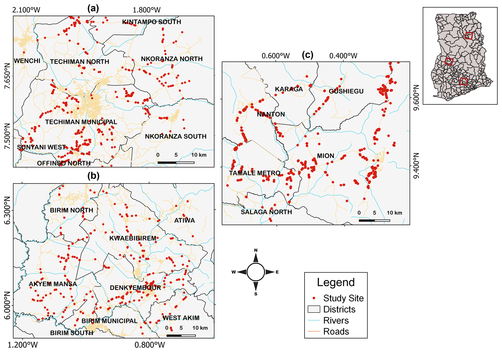
Figure 1 Locations of samples for crop-type mapping in the 2020 extensive campaign. (a) Transition zone and (b) Deciduous and (c) Northern Savannah sites. The top right sub-image shows the locations of these areas within Ghana.

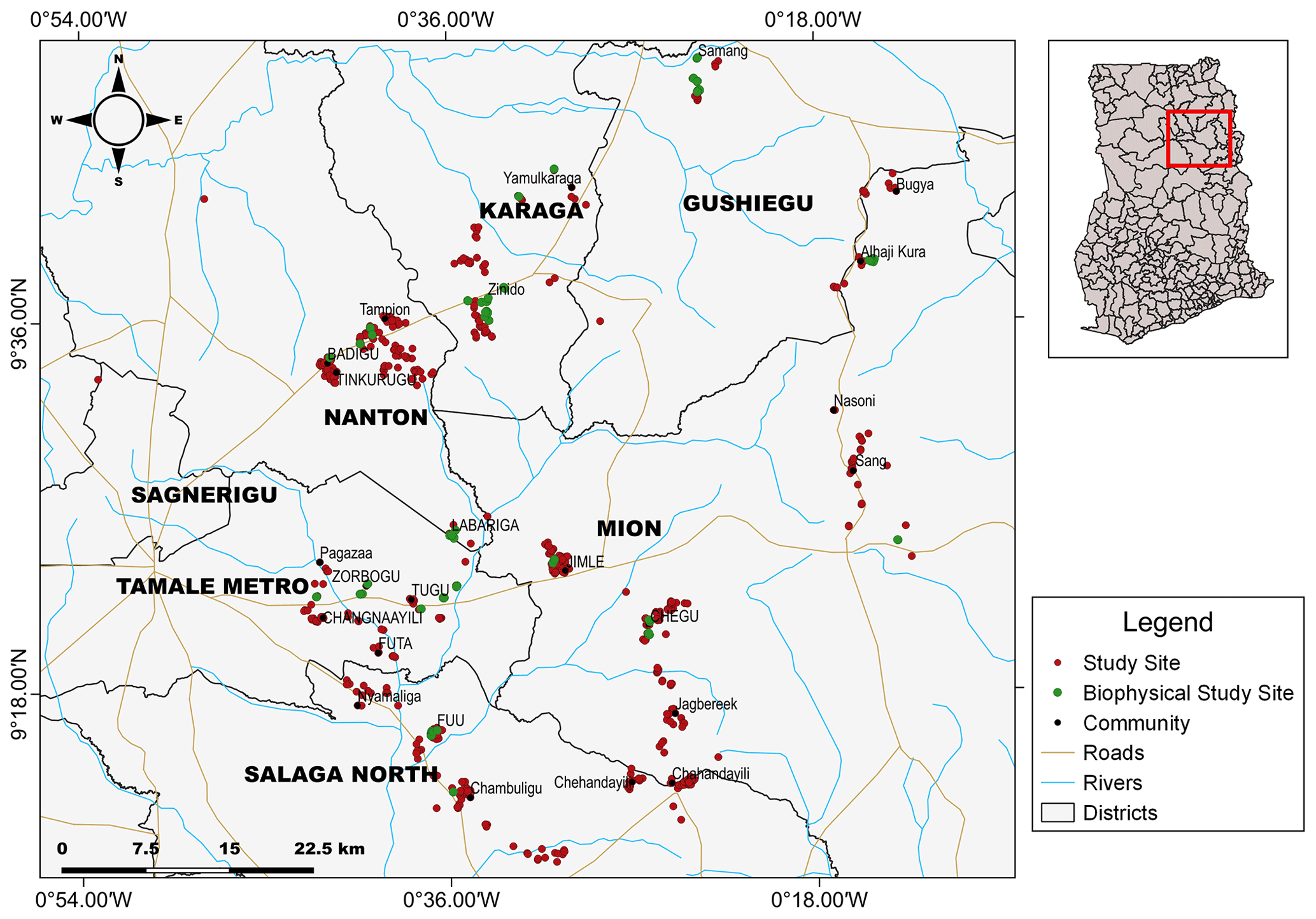
Figure 2 Location of the crop-type mapping for the 2021 campaign. Red dots show agricultural fields. Green dots show locations where biophysical parameters were collected. The top right sub-image shows the location of the area within Ghana.

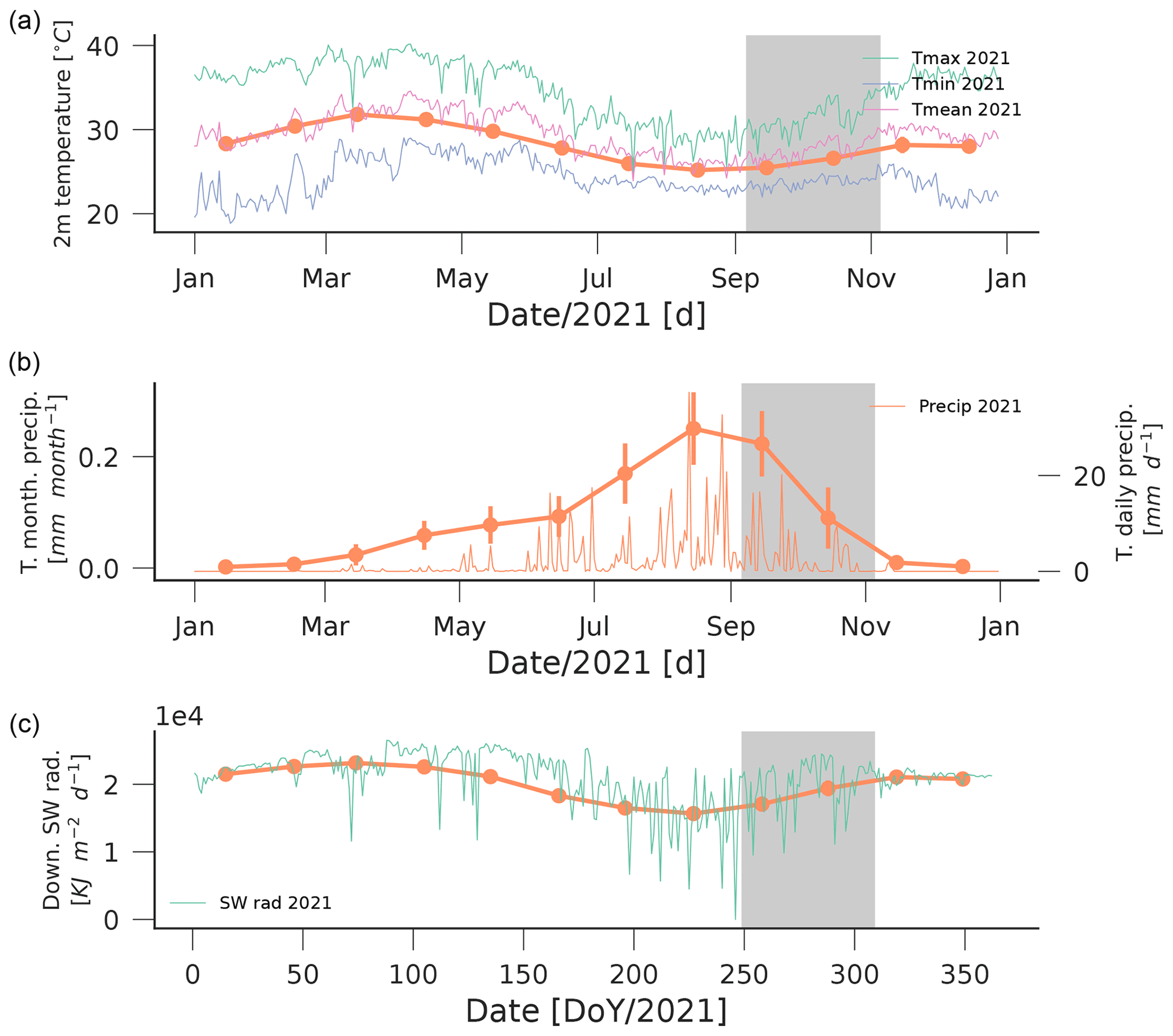
Figure 3 Monthly climatologies for temperature (a), precipitation (b) and shortwave downwelling radiation (c) over the Tamale area (derived from the ERA5/Land data set between 1990 and 2021) as well as daily temperatures, precipitation and downwelling radiation for 2021. The grey area indicates the biophysical parameter collection period.

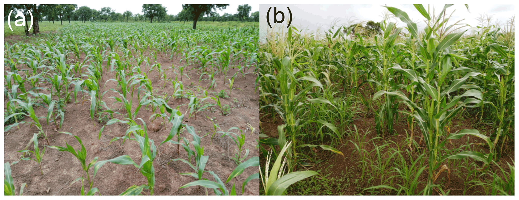
Figure 4 Pictures of two maize fields within the study area, showing the crop heterogeneity and presence of weeds and trees within fields. (a) Field 7071ZIN (17 September 2021) in situ LAI: 1.1 m² m⁻², chlorophyll conc.: 39.3 µg cm⁻². (b) Field 3075TAM (14 September 2021) LAI: 1.9 m² m⁻², chlorophyll conc.: 45.2 µg cm⁻².

2.2 Crop-type mapping

Two crop-type mapping campaigns were conducted: a preliminary campaign in December 2020, covering three agroecological zones, and a maize-focused campaign in 2021.

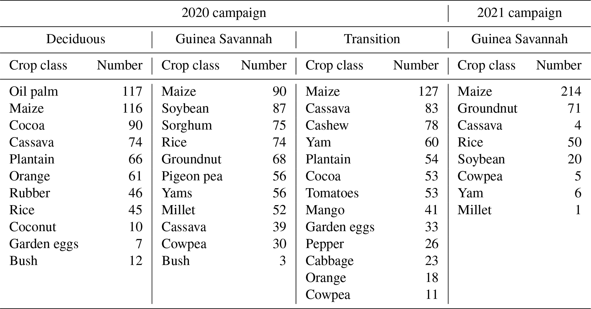
The 2020 campaign served partly as a training exercise for 2021 data collection but also to provide extensive sampling over different crops and cropping systems within Ghana. Three teams surveyed three ∼ 50 km × 50 km sites in the Guinea Savanna, Transition and Deciduous forest regions (see Fig. 1 for the locations) between 12 December and 21 December 2020. The site locations and main crops associated with each site were chosen based on previous knowledge and in discussion with local agricultural extension workers. Within each site, crop types were initially identified from a drive-through “windshield survey” (Defourny et al., 2014), and GPS locations and photographs were simultaneously gathered using mobile phones inside individual fields. Crop type was mapped at a point location within each field. Fields that were less than 0.25 ha were ignored, following the recommendations from Defourny et al. (2014). Fields were selected for cases where (i) a crop could be identified (the campaign took place in December, when many fields had already been harvested, so crop identification was sometimes based on crop residue inspection) and (ii) a single crop was present (so plots with evidence of intercropping were discarded). The crop types to map were selected as being the most representative of the region, with the goal of collecting around 600 points for each region. The crop distribution per region is shown in Table 1. For the Deciduous, Savannah and Transition zones, 644, 630 and 660 fields, respectively, were sampled.

A second crop-type campaign was carried out in August 2021, more focused on identifying maize fields. It was conducted near Tamale (Guinea Savannah region) (Fig. 2), with the primary aim of identifying maize fields to compare to the data collected in 2020 and the secondary aim of scoping fields that could be used for the biophysical parameter campaign. Fields were selected following the same considerations as the 2020 campaign, but rather than points, polygons of the field boundaries were collected. This required physical access to the fields, for which access permission was needed from the owners. This resulted in a smaller number of fields (375) being surveyed compared to the 2020 campaign (Table 1). Field boundaries were collected by walking around the field using a GPS tracker and taking care to exclude trees and buildings to ensure that the mapped field area was as homogeneous as possible and measurements in that area would relate to the crop. Only minor post-collection editing was performed (e.g. closing polygons).

Table 1 Number of mapped fields per crop-type class for the 2020 and 2021 campaigns.

2.3 Biophysical parameter collection

The collection of biophysical parameters in 2021 focused on maize farms around Tamale. These farms were selected from maize fields mapped in 2021 (Sect. 2.2) after permission was obtained from the farmers to allow repeated visits and harvesting at the end of the growing season. The field campaign was delayed by the arrival of the measurement equipment in Ghana and training requirements (Covid and related delays), so the fields that were selected were those that appeared to be less developed towards the start of the measurement campaign (August 2021). In the study area, maize is typically sown around June, so it is possible that the selected fields are sown later than what is usual for this area. As for the crop mapping, the selected fields show no intercropping, and the presence of trees is limited to the edges and has been masked out. These decisions limit the selection of fields but provide a simpler setting to validate EO-derived products and to test the link between biophysical parameters and crop production. Heterogeneous fields required different measurement strategies to characterise the nature of the crop combination, and the presence of several canopy layers (e.g. crop–tree) is not considered in most EO LAI products, so tree detection and masking using very high-resolution (VHR) data would be needed to make any comparison fair.

An initial set of 56 maize fields was selected for both biophysical parameters and yield characterisation. The field sizes ranged from 0.25 to 2.2 ha, with an average field size of 0.78 ha. From the initial 56 farms, 8 farms were dropped later in the season as the crop had been damaged by animals, flooded or abandoned by the farmer and overgrown with weeds. These fields are representative of typical maize fields grown in the Guinea Savannah region of Ghana.

Measurements were taken from 6 September 2021 to 5 November 2021. Measurement of LAI and leaf chlorophyll content was performed weekly on the sample farms using an Li-Cor LAI-2200-C device and a Minolta SPAD 500 device, respectively. The full field protocol for LAI and leaf chlorophyll is presented in Appendix A.

In each field visited, four locations were selected and marked and measurements taken at these. For the leaf chlorophyll measurements, the fifth and sixth leaves (relative to the bottom of the canopy) of individual plants in each sampling site were tagged on the first visit. Measurements were then repeatedly taken on these leaves in subsequent visits. At the time of measurements, the general state of the crop and its phenology were also noted.

2.4 Crop yield and biomass measurements

Crop yield was measured by crop cutting. For each farm, three 6 m × 6 m plots inside the field were harvested, cobs removed, and grain weighted. We report the quadrant yields as well as the field-averaged mean yield and associated standard deviation. For a subset of 10 farms, above-ground biomass was also sampled. The full protocol is given in Appendix B.

2.5 Satellite data

Together with the ground data described above, we have also produced a ready-processed data set of contemporaneous satellite observations to facilitate training and experimentation. We will use the ground data to develop an empirical estimation of LAI. Figure 5 shows time series of the field-averaged normalised difference vegetation index (NDVI) over four fields derived from Sentinel 2 and Planet. Sentinel 2 observations are restricted by clouds, whereas Planet data are more frequent, particularly towards the end of the growing season. When both sensors collect data, the NDVI value is comparable, although it is also clear that the Planet data show a larger instability in time as well as the presence of outliers. It would have been preferable to use Sentinel 2 observations to produce estimates of LAI as the data have a richer spectral information content, but given the scarcity of matchups with the ground measurements, we decided to use the Planet data and to develop a simple mapping using a vegetation index as a pragmatic trade-off.

We have used the Planet Surface Reflectance (SR) version 2 product (Planet, 2018) downloaded from Planet Explorer (https://www.planet.com/explorer/, last access: 16 November 2022). We calculate the NDVI as it is a commonly used vegetation index that is frequently used to describe crop condition and yield (Turner et al., 1999; Smith et al., 2002; le Maire et al., 2004; Ferwerda and Skidmore, 2007; le Maire et al., 2008). The Planet SR product is derived from the top-of-atmosphere (TOA) radiance images acquired by the PlanetScope constellation which collects data in the red, green, blue and near-infrared bands with a nominal resolution of ∼ 3.7 m. The SR product has a ground sampling distance of 3 m and a positional accuracy better than 10 m (Planet, 2018). The data are atmospherically corrected and have an associated cloud, cloud shadow, etc., pixel mask (Planet, 2018).

The vast changes in acquisition geometry, sensor properties, failure of the cloud and cloud/shadow mask and inconsistencies in the atmospheric correction result in the measurements from Planet being very noisy and contaminated with outliers, as is clear from Fig. 5 (see also Houborg and McCabe, 2016). Outliers and gaps in the time series (particularly at the start of the measurement period) require treatment: we develop here a robust smoothing and interpolation approach that allows us to achieve the desired NDVI-to-LAI mapping along with an estimate of LAI uncertainty.

We use an efficient and robust smoothing filter with a bi-square weighting to flag and remove gross outliers in the Planet NDVI time series (Heiberger and Becker, 1992; Garcia, 2010). An outlier is flagged if $\left|\frac{u_i}{\mathrm{4.685}}\right|\ge \mathrm{1}$, where u_i is the studentised residual for sample i (Garcia, 2010). An example application of the smoother is shown in Fig. 6a, where the Sentinel 2 field-averaged NDVI is also shown for comparison.

To further reduce the large remaining variability, we fit a double-logistic function (Zhang et al., 2003; Beck et al., 2006; Atkinson et al., 2012; Yang et al., 2019) (Eq. 1) to NDVI as a function of time t for each pixel, an effective way to both reduce the noise (Hird and McDermid, 2009; Jönsson and Eklundh, 2002) and allow temporal interpolation.

$$\begin{array}{}\text{(1)}& \begin{array}{rl}\text{NDVI}& =p_{\mathrm{0}}-p_{\mathrm{1}}\left[{\displaystyle \frac{\mathrm{1}}{\mathrm{1}+\exp \left(p_{\mathrm{2}}\right(t-p_{\mathrm{3}}\left)\right)}}\right.\\ & \left.+{\displaystyle \frac{\mathrm{1}}{\mathrm{1}+\exp (-p_{\mathrm{4}}(t-p_{\mathrm{5}}\left)\right)}}-\mathrm{1}\right]\end{array}\end{array}$$

We have implemented the double-logistic fitting as a two-stage process to account for both the large variability and the limited observational opportunity at the early start of the growing season. As a first stage, the six parameters p_i, i∈(0…5) in Eq. (1) are estimated for individual pixels over a field. Then, the per-field median values for the six parameters are calculated and used to define bounds in parameter values for the second pass. In the second pass, the double logistic is again fitted to the per-pixel NDVI time series, with all parameters except p₁ (the amplitude) being constrained to be within 5 % of the median field value. In this way, we ensure that the mapped timing information is spatially correlated at the field level and that the variation in the amplitude of the vegetation index will be greater.

Although the outlier filtering method described above is based on smoothing and statistical tests, the spatially aware field constraints and typical consistency in reconstructed VI trajectories (Fig. 6c) over a field suggest that the outlier filtering is appropriate and does not introduce large biases. The processing described above results in more stable estimates of NDVI over time, as can be seen in Fig. 6c, particularly tightening up the temporal trajectory towards the start of the time series.

We use the interpolated and smoothed NDVI data to develop the mapping to the LAI. The large uncertainty in the individual elemental sampling unit (ESU) LAI ground measurements suggests that the model is fitted at field level. Potential further issues with a mapping from NDVI to LAI are saturation effects with high LAI (Baret and Guyot, 1991). For maize in the study area, a very high LAI is never achieved, and the field measurements never exceed an LAI of 3, so we might suppose that saturation of the signal should not be a problem here. The limited range of the field LAI data also suggests that a linear model is an acceptable model choice. We estimate the value of NDVI on the day of the in situ observations from the smoothed/interpolated Planet data and average both the EO-estimated NDVI and the in situ LAI over the field. We randomly split the data set into 70 % for training and 30 % validation. We fit the linear model $\text{LAI}=m\cdot \text{NDVI}+c$ to the training data and test its performance on the validation samples. We repeat this fitting procedure using 20 random splits to avoid biases in the estimates of m and c and to provide an initial uncertainty in these parameters.

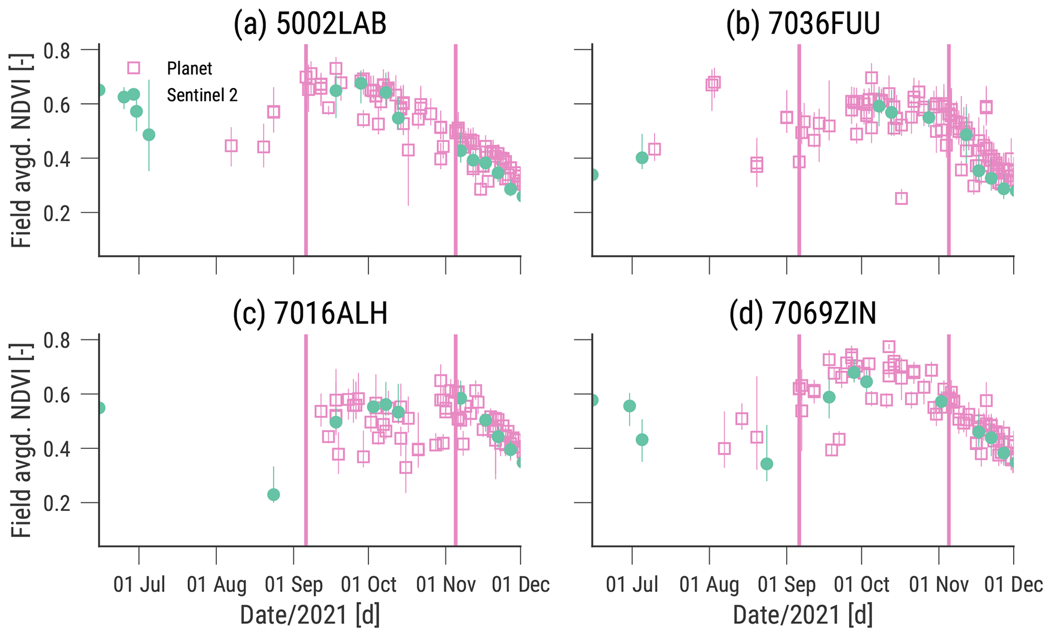
Figure 5 Field-averaged NDVI from Sentinel 2 (green dots) and Planet (purple squares) over four of the visited maize fields in 2021. Vertical purple lines indicate the extent of the in situ data-gathering campaign. Error bars indicated 2 %–98 % field NDVI percentiles.

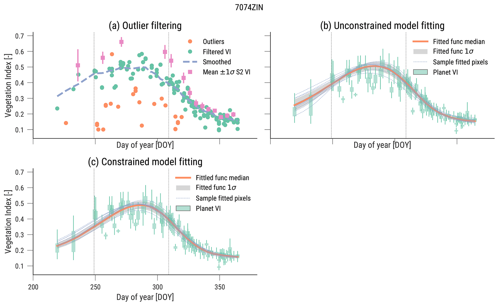
Figure 6 Planet VI time series processing step example for field 7074ZIN. (a) Outlier filtering. (b) First-pass single-pixel double-logistic fitting (unconstrained). (c) Second-pass single-pixel double-logistic fitting (phenology parameters constrained by the median field). The vertical lines show the extent of the ground campaign period.

2.6 Validation of cropland masks

We use the collected data to partially validate the Digital Earth Africa cropland mask (Burton et al., 2022). This binary (crop/no-crop) mask has been developed for 2019, but there are plans to extend it to other years. Using crop masks from prior years is a pragmatic choice to monitor the same region in the current season (Becker-Reshef et al., 2018). We can use the crop location data to assess the accuracy of the crop mask for other years and to test its suitability to enable within-season crop mapping. The Digital Earth Africa cropland mask is based on a random forest (RF) classifier, but as a binary mask of the cropland/non-cropland final product, it provides an estimate of the probability of each 10 m pixel being cropland. The final binary mask is derived from the pixel probability data set, and cropland is assumed if the pixel probability is greater than 0.5. We can assess the quality of the mask by testing the fraction of surveyed cropland locations (pixels) and their associated probability. A good mask would be characterised by a large proportion of the visited cropland pixels having a probability larger than 0.5. Conversely, a poor mask would show most visited pixels having a probability lower than 0.5.

2.7 Crop mask classification

The data sets collected in 2020 and 2021 can be used to extend previous efforts to provide cropland/crop-type maps (Xiong et al., 2017; Jolivot et al., 2021; Estes et al., 2022; Burton et al., 2022), but here we illustrate the use of the 2021 data set in developing a 10 m maize mask for the whole Northern zone in Ghana using data from Sentinel 2. The classification experiment is done using the Google Earth Engine platform (Gorelick et al., 2017). The approach taken was to collect Sentinel 2 observations of surface reflectance (atmospherically corrected with the sen2cor package, Louis et al., 2016, GEE data set “COPERNICUS/S2_SR”) between May and October 2021, when rain-fed crops are being grown. After applying a cloud mask and only processing pixels labelled “Crops” in the ESRI Sentinel 2 land cover map (Karra et al., 2021) (although the code provided is flexible and users can modify the base map and its classes easily), temporal series of a number of vegetation indices (NDVI, LSWI, IRECI and GCVI) and a subset of spectral bands (Red Edge 1, NIR, SWIR1 and SWIR2) are then smoothed/interpolated using a robust Whittaker smoother (Eilers, 2003; Garcia, 2010), with a smoothing strength parameter of 0.5. The classifier used was a random forest with 100 trees, and in order to train the classifier, the individual pixels underlying the field-surveyed polygons were used. The pixels were split into two sets: 70 % and 30 % of the points were used for training and validation (respectively). For the production of the final mask, all pixels were used to train the classifier.

3 Results

3.1 Biophysical parameter measurements

Pictures from two typical fields are shown in Fig. 4, which show the clear row structure and the low plant density that was common to most fields. Time series of the evolution of in situ measurements are shown in Figs. 7 and 8 for LAI and chlorophyll, respectively, for the sample fields.

LAI values ranged from 0.1 to 5.24 m² m⁻², with a mean value of 1.37. The 10th, 50th and 90th percentiles were 0.5281, 1.15 and 2.13 m² m⁻², respectively. LAI values are lower compared to other regions where irrigation and fertilisation are common but are in line with other studies for the area (Srivastava et al., 2016; MacCarthy et al., 2015). In some of the fields the decrease in LAI from around its maximum is obvious (e.g. fields labelled 1029ZIN, 5034TUG, 5036TUG and 1056ZIN). The pattern for other fields is not clear, with some having the LAI peak towards day of year (DoY) 275 (e.g. fields labelled 7021YAM, 7068ZIN and 7069ZIN), whereas other fields show no clear dynamics.

For leaf chlorophyll concentration, the values ranged between 6.1 and 60.3 µg cm⁻², with a mean value of 34.2 µg cm⁻² and the 10th, 50th and 90th percentiles given by 15.71, 35.9 and 49.39 µg cm⁻².

The trends for leaf chlorophyll concentration are clearer than those of the LAI. Most fields show an expected decay of chlorophyll as the season progresses, with most of the differences between fields relating to the timing and magnitude of the leaf chlorophyll reduction.

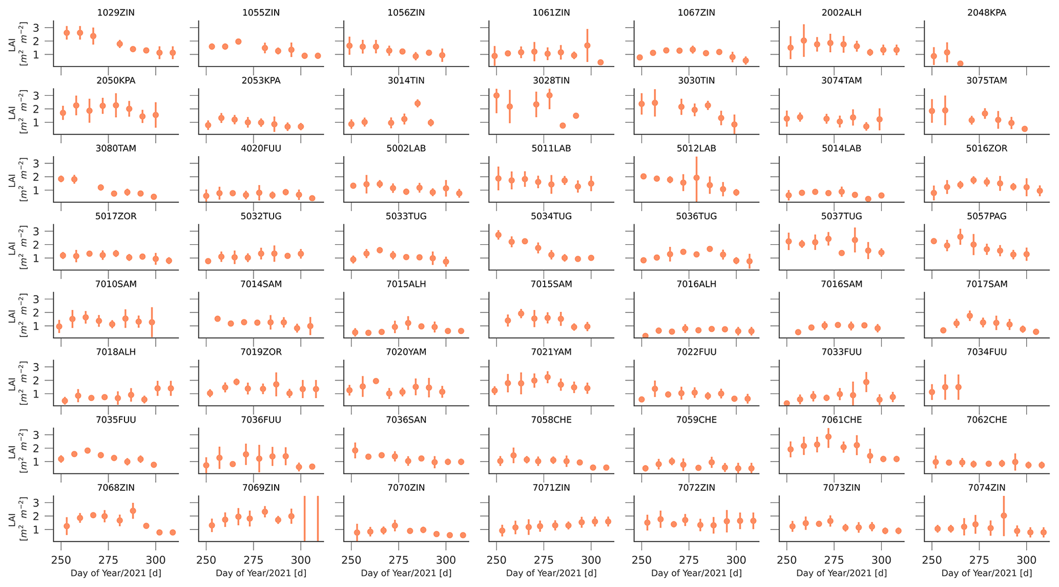
Figure 7 Per-field temporal evolution of the in situ leaf area index (LAI). For any date, the mean is shown, and error bars represent ±1σ.

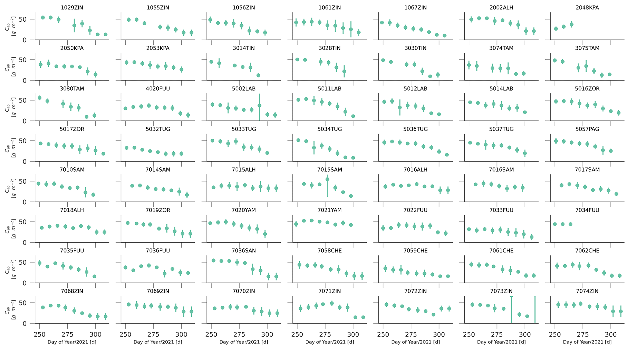
Figure 8 Per-field temporal evolution of in situ leaf area chlorophyll concentration (C_ab). For any date, the mean is shown, and error bars represent ±1σ.

3.2 Crop yield and biomass measurements

The distributions of measured yield are shown in Fig. 9a, c. Biomass and harvest index histograms are shown in Fig. 9b, d. For the individual quadrant measurements, yields varied between 35 and 5036 kg ha⁻¹. The per-field averaged values were between 190 (field 7033FUU) and 4580 kg ha⁻¹ (field 7021YAM), with an average of 1379 kg ha⁻¹ and a standard deviation of 872 kg ha⁻¹. The uncertainties within the fields were also important, with an average within-field standard deviation in yield of ∼350 kg ha⁻¹. Total above-ground biomass was between 1000 and 16 000 kg ha⁻¹, and the harvest index varied between 0.21 and 0.77.

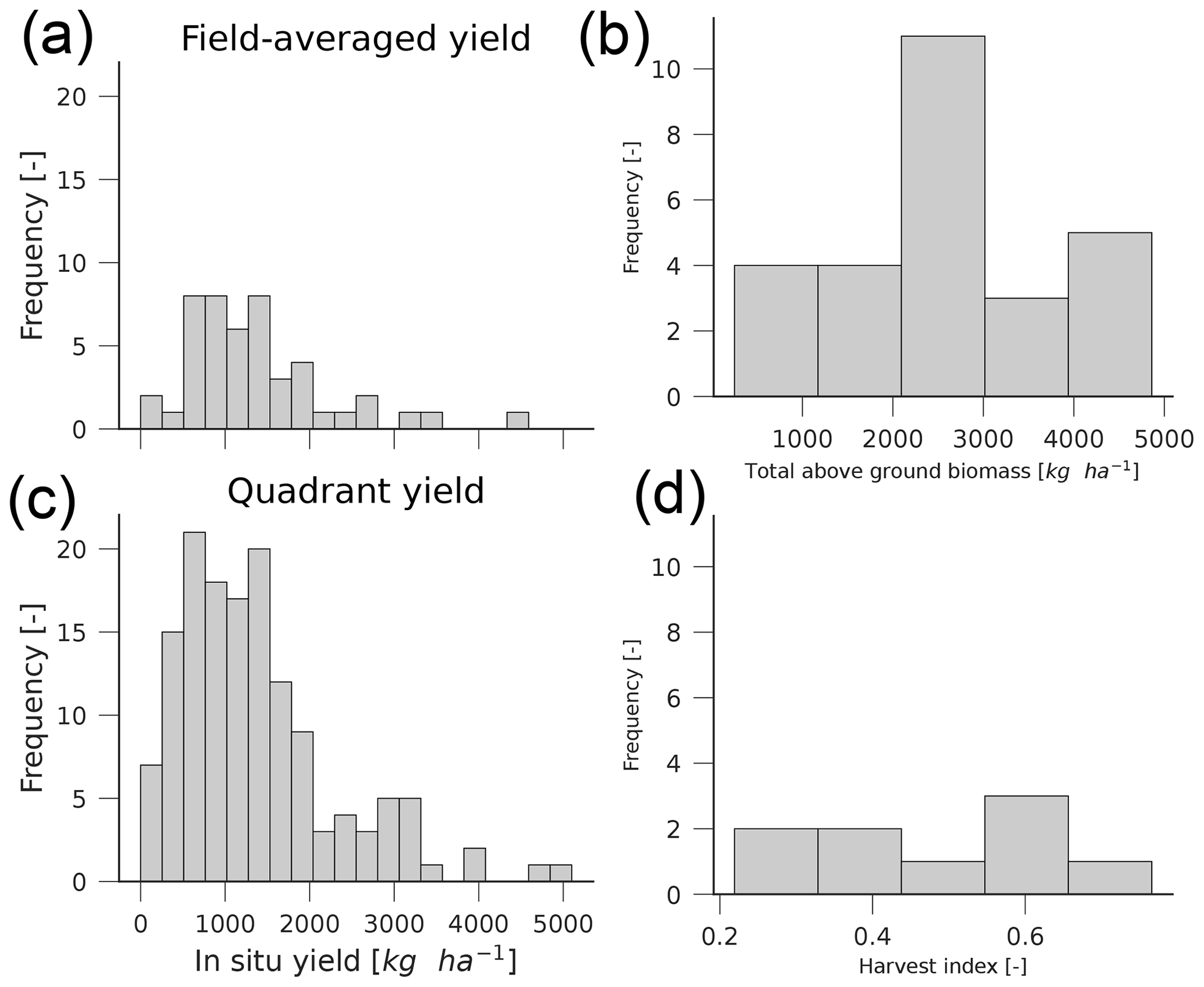
Figure 9 Crop yield distribution (a: field-averaged, c: individual quadrants), field-averaged above-ground biomass (b) and field-averaged harvest index (d).

3.3 EO-derived LAI

The approach described in Sect. 2.5 results in a simple transformation between Planet NDVI and LAI. The calibration and validation of this approach are shown in Fig. 10. The conversion equation is given by ${\text{LAI}}_{\mathrm{pred}}=\mathrm{3.95}\cdot \text{NDVI}-\mathrm{1.21}$, with the two coefficients having bootstrapped uncertainties of 0.16 and 0.09, respectively. In validation, the model shows a modest correlation (R=0.5, R²=0.25), but in absolute terms, the model performs in line with medium-resolution products (Fang et al., 2019), with a validation root mean squared error (RMSE) around 0.43 m² m⁻², a mean absolute error (MAE) of 0.35 m² m⁻² and a negligible bias (Fig. 10). Figure 10 clearly shows an underestimation of the Planet NDVI signal for LAI>1.5. A comparison of the field LAI measurements and the Planet-derived LAI time series is presented in Fig. 11, where a correspondence between the model-predicted LAI and the field measurements is shown.

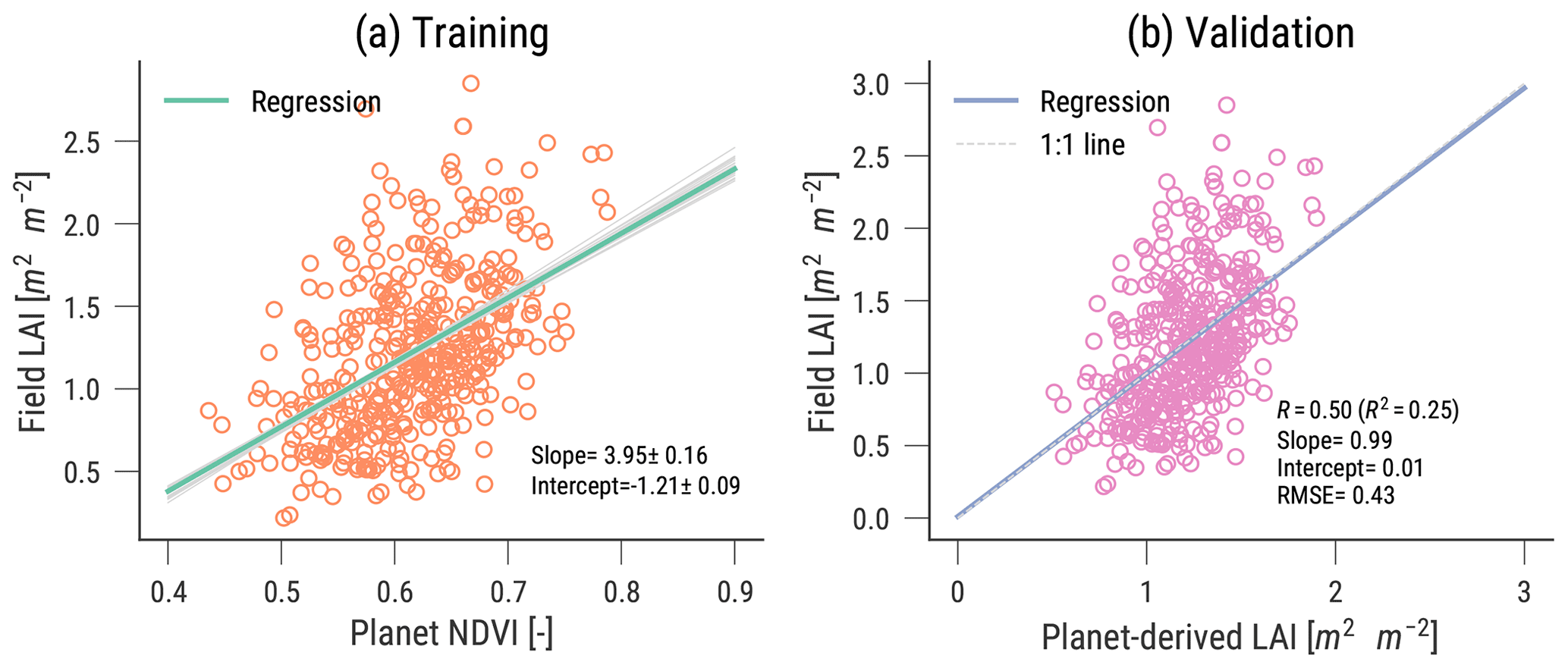
Figure 10 NDVI-to-LAI calibration (grey lines show bootstrap uncertainty) (a) and validation (b).

Figure 11 Predicted LAI time series and associated standard deviation (blue line and grey area) in comparison with field measurements (per-field mean and standard deviation, green lines).

3.4 Validation of cropland masks

Figure 12 shows the distribution of Digital Earth Africa's cropland mask probabilities for the surveyed pixels in 2020 and 2021. For a perfect mapping, one would expect the cumulative distribution to be a Heaviside step function changing from 0 to 1 for a high probability value, suggesting that all the pixels are detected as cropland with a high confidence. At the very least, the change point should be around 50. Any samples that appear with less than 50 % probability would be omission errors.

There are clear differences between years and sites. For the semi-deciduous zone in 2020, the vast majority of pixels are labelled non-crop, with the cropland mask consistently underreporting crop area. The best results are obtained for maize, cassava and plantain, where ≈12 % of the crop area is reported as such. For the Transition zone in 2020, the performance is better. For pepper, cowpea and cabbage, ≈50 % of the surveyed pixels are reported as cropland. For maize in this region, only 40 % of the pixels have a probability of more than 0.5. Results for the Savannah region in 2020 are better: ≈60 % of maize fields are labelled cropland, but for other popular crops such as sorghum, millet, groundnut and soybean, less than 40 % of the samples are labelled cropland. For the Savannah region in 2021, the results are similar to the same region in 2020, with rice and maize having around half of the pixels detected as cropland by the mask. Soybean is only detected in 20 % of the pixels. The conditions towards the south of Ghana (persistent cloud, mixing of crops and trees) make it harder to identify cropland. Towards the north, with fewer trees and (comparatively) less cloud, the cropland mask improves but still misses around half of the cropland area, and for some crops (soybean), the situation is even worse.

It is worth noting that, for 2020, each pixel belongs to a different field, whereas for 2021, all pixels belonging to the visited fields have been considered, and as such, pixels within a field are spatially correlated, which suggests that the result for this site is probably optimistic. An example of the cropland mask and the visited fields around a small area within the Mion district is shown in Fig. 13, where it is clear that the cropland mask misses many of the visited fields. The reported probabilities of cropland values are also fairly low (very few pixels have probabilities over 70 %), suggesting a large uncertainty for most pixels.

Our results are hard to compare with the official validation report from Burton et al. (2022), as we are considering using the mask for different periods than those used to develop the data set, but in our case, the results show a large omission error of more than 50 % for all the crops, with the results being markedly worse towards the south of Ghana. These figures are at least double the reported 25 % omission reported in Burton et al. (2022).

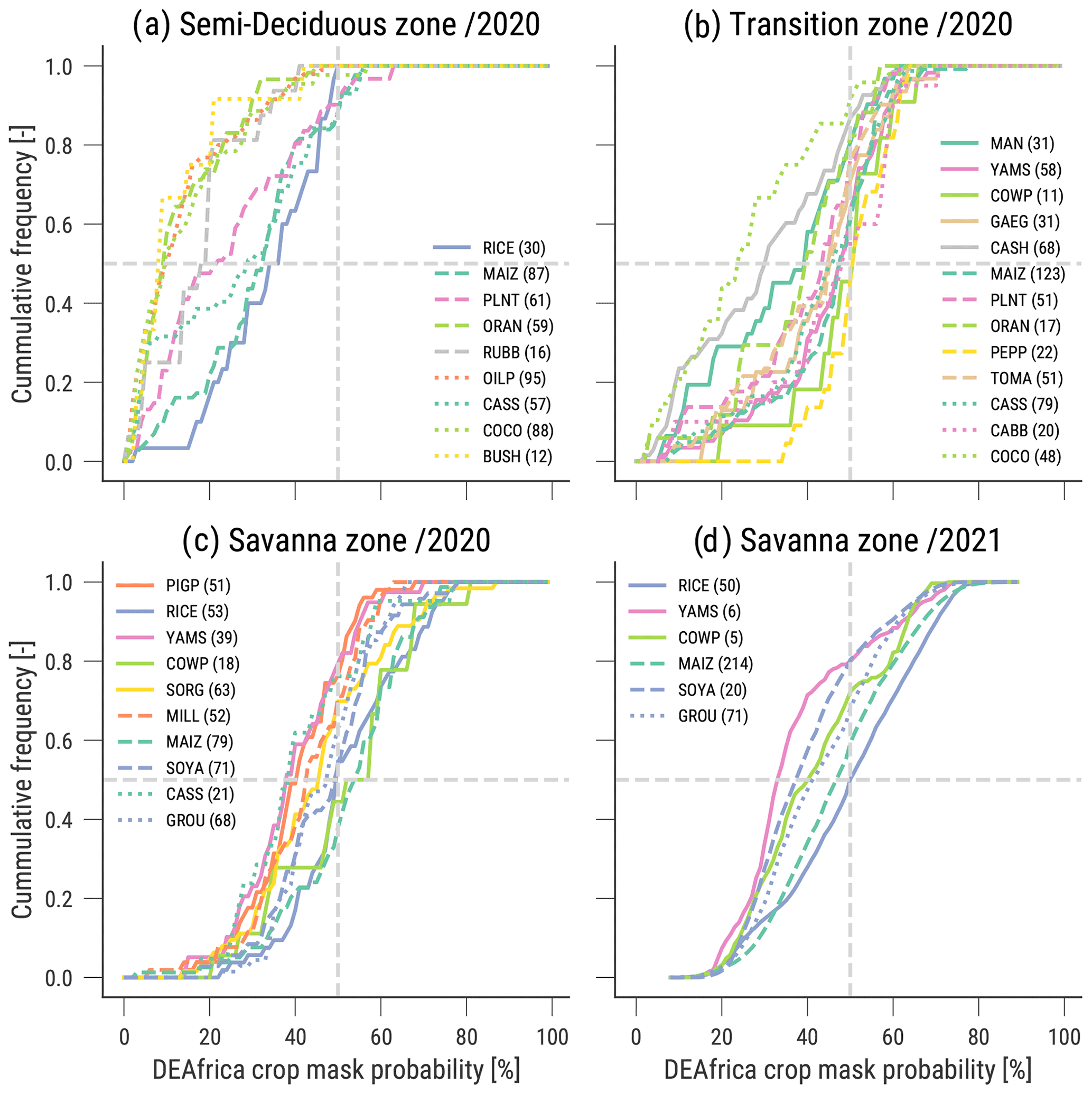
Figure 12 Cumulative frequency of surveyed pixels against the probability of cropland per Digital Earth Africa cropland probability mask for 2019. Horizontal dashed lines are 0.5, and the vertical line is a cropland probability of 50 %. Numbers between brackets in legends indicate the number of samples of each class included in the calculations.

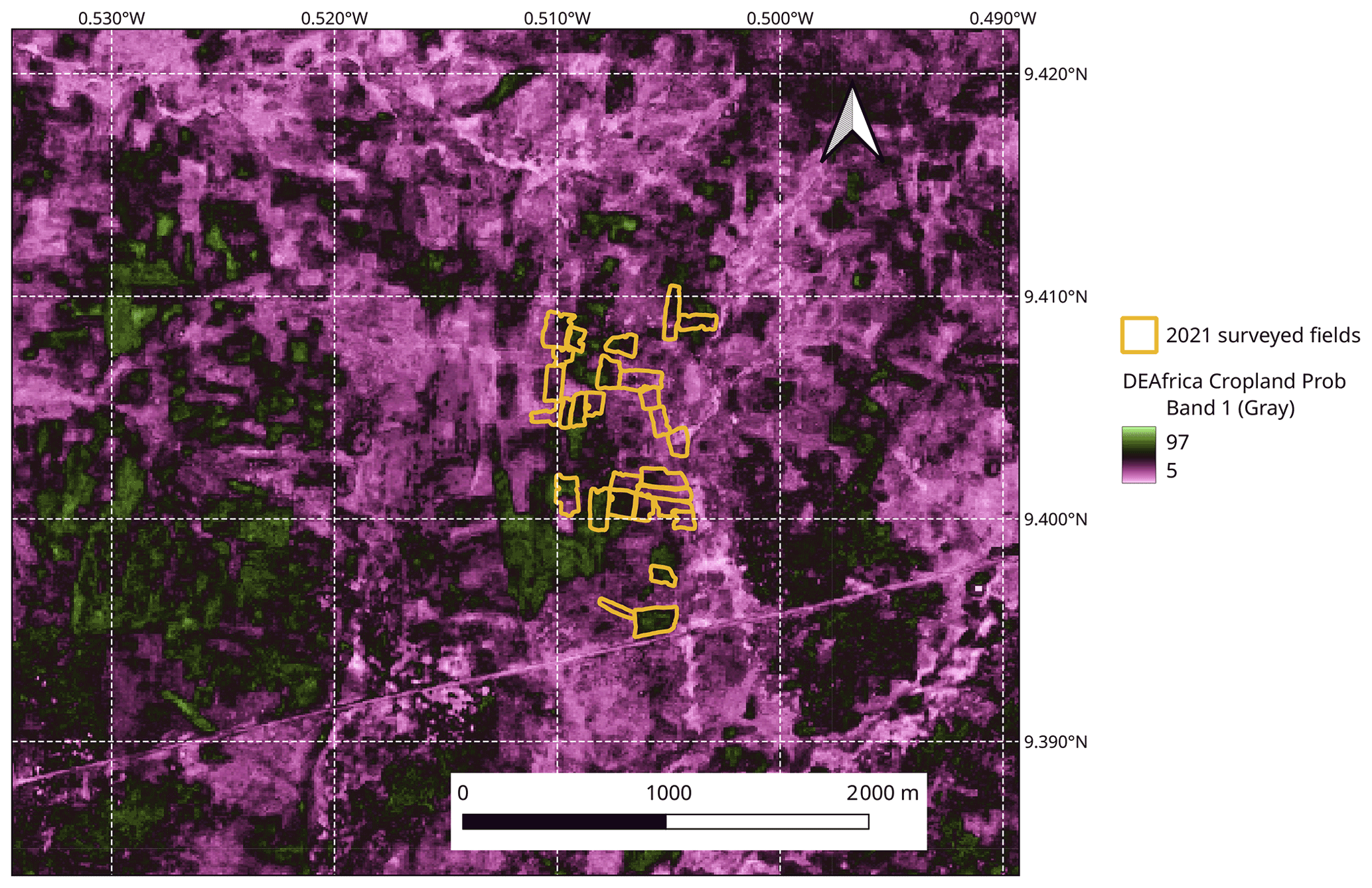
Figure 13 Detail of some of the visited field sites (yellow polygons) and the Digital Earth Africa cropland probability mask (Burton et al., 2022) around the Mion district in the Northern zone in 2021.

3.5 Crop-type classification

The maize mask derived as presented in Sect. 2.7 is shown in Fig. 14. The validation results (using the 70:30 data split introduced earlier) were an overall accuracy of 0.84 and a kappa score of 0.68 (see Table 2 for details). Five-fold cross-validation was also used to evaluate the robustness of the results shown in Table 2, which resulted in an overall accuracy of 0.72 (standard deviation 0.12). The importance of each considered feature is shown in the Gini index plot shown in Fig. 15, which ranks different features by classifier importance.

Table 2 Results from the crop classification for 2021.

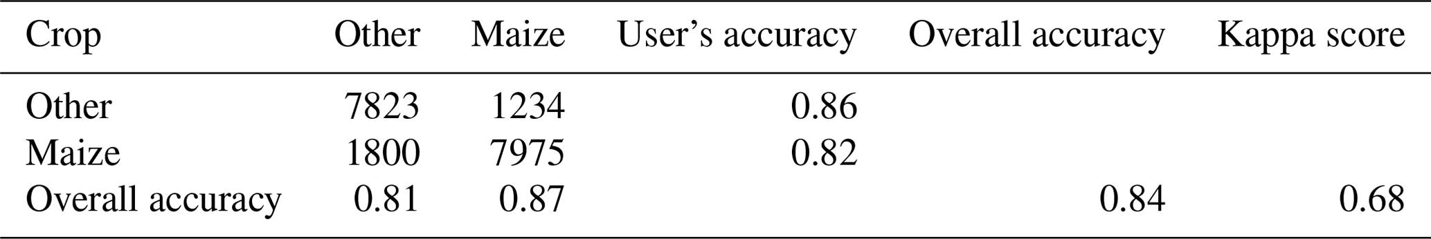
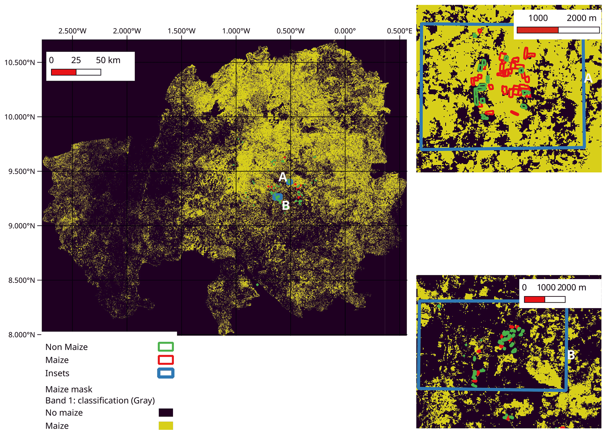
Figure 14 Left panel: maize mask (maize shown in orange). Insets (A) and (B) illustrate the field data. Maize fields are shown as green outlines and other crops as red outlines.

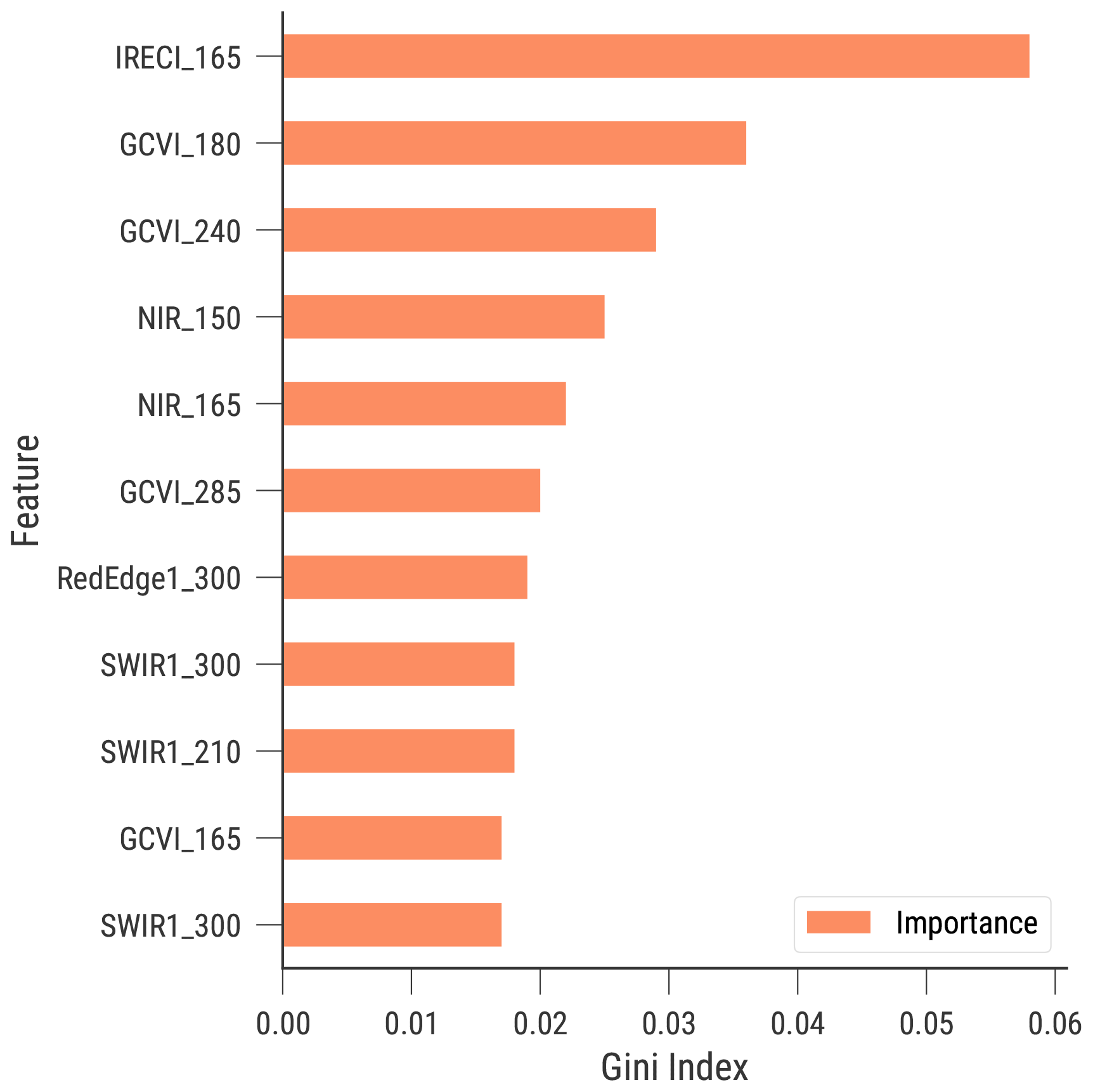
Figure 15 Gini index for the random forest maize mask classifier, showing the 10 highest-ranking features in the classifier. Features are given by their abbreviation, followed by time step. For example, IRECI_165 represents the IRECI at day of year 165.

3.6 Yield prediction testing

The relationship between leaf area and crop yield has been widely explored, often via vegetation indices (e.g. Becker-Reshef et al., 2010), and it usually follows that a green, healthy and dense canopy results in a higher yield. Many authors relate yield to the magnitude of the maximum value of the leaf area (or vegetation) index. This is a fairly crude relationship, but for regional applications in areas with large fields and monocultures, it can be quite effective (Mkhabela et al., 2011; Petersen, 2018; Kouadio et al., 2012). Here, we look at this relationship between maximum field-measured LAI and field-measured yield as well as Planet-derived LAI and field-measured yield. For in situ data, a linear relationship yields a reasonable fit (coefficient of correlation R=0.66, coefficient of determination R²=0.44) once fields 7021YAN, 7033FUU and 7036SAN are removed as outliers. The slope and intercept of the linear model are 866.44 and −180.45, respectively (Fig. 16a). Including the left-out fields reduces the coefficient of determination to R²=0.31. Using the maximum LAI value from the Planet data introduced in Sect. 2.5, the correlation degrades to R=0.53 (R²=0.29, ignoring fields 7021YAN, 7033FUU and 7036SAN) (Fig. 16b). Slope and intercept for the Planet-derived maximum LAI are 1606.51 and −893.10, respectively. The lower correlation from the satellite-derived relationship is probably explained by the underestimation of the maximum LAI for the higher yield fields (Fig. 10). For the in situ case, the value of the slope in the maximum LAI relationship is close to 900 kg ha⁻¹, suggesting that, with errors in the Planet LAI estimates of around 0.44 m² m⁻², the typical error in the estimate would be around 381 kg ha⁻¹, a value close to the average uncertainty in the field-measured yield.

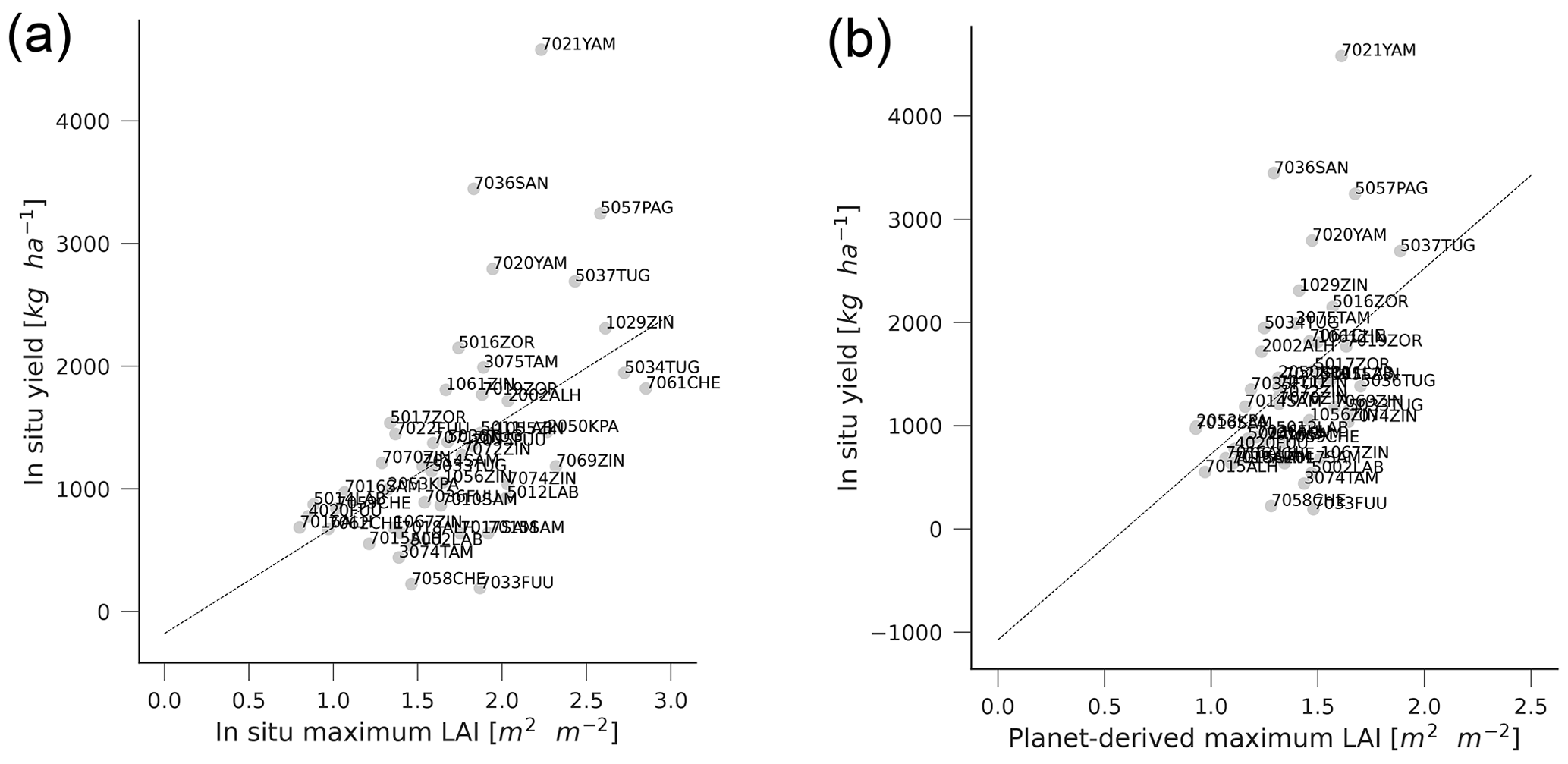
Figure 16 Relationship between maximum LAI estimates and yield. For in situ measured LAI vs. yield (panel a), and discarding fields 7021YAN, 7033FUU and 7036SAN, the linear fit has R²=0.44, and the linear fit is shown as the dotted line $y=\mathrm{866.33}\cdot x-\mathrm{180.45}.$. For Planet-derived LAI vs. yield (panel b), and discarding fields 7021YAN, 7033FUU and 7036SAN, the linear fit has R²=0.28, and the linear fit is shown as the dotted line $y=\mathrm{1606.51}\cdot x-\mathrm{893.10}$.

4 Discussion

4.1 Crop measurements

The in situ data gathered are a useful contribution to advancing crop-monitoring methods for smallholder farmers in western Africa. It is important to note that the data collection started when the crops were already established in the fields, as is clear from the satellite temporal trajectories (e.g. Figs. 6 and 4), so that the initial growth period after emergence was not captured. Additionally, due to logistical issues, the field campaign could only start towards the end of August/start of September 2021, when planting in this area started 3 months earlier. To capture the longest possible dynamics over the campaign, the chosen fields were all late-sown, which may result in them not being very representative of the majority of fields in the region. The choice of fields with the least amount of tree cover and no intercropping may also impact the generality of the data gathered with respect to other fields where these conditions are not met. The in situ LAI measurements show some variability (mean standard deviation for samples collected on the same date in the same field of ≈0.25 m² m⁻²). The effect of this variation is relatively more important here as the maximum LAI is quite small (≈2 m² m⁻² compared to e.g. the US, where the maximum LAI will be between around 5 and 6 m² m⁻² (Nguy-Robertson et al., 2012)).

The variation of leaf chlorophyll content appears different to the LAI trajectory but is broadly characterised by a plateau followed by a steady drop. Here, we have not looked at its use, either for EO-product validation or other applications, as the scarcity of Sentinel 2 reflectance data over the fields makes retrievals unreliable.

There is a large variability of yields within individual fields. This is due to differential management practices and small-scale soil and/or topography variations. Three crop cuts over a standardised area were used to determine yield, conforming to common practice. However, the spatial locations of these estimates were not surveyed, so the data limit us to answering whether EO data provide useful within-field yield variability. Yield estimates should also be co-located with the LAI/leaf chlorophyll measurement points to fully exploit the connection between canopy variables and yield.

Only limited data on above-ground biomass were collected, but the distribution of the harvest index between 0.2 and 0.7 suggests that the relationship between biomass and yield is not well established. Lambert et al. (2018) find a strong relationship between above-ground biomass (AGB) and yield for maize in Mali. Karlson et al. (2020) show that, for a range of cereals, the relationship varies from year to year in Burkina Faso. Hay and Gilbert (2001) show a harvest index (HI) ranging from 0.19 to 0.53 for maize in Malawi. It is interesting that Moser et al. (2006) point out that water stress can have an impact on HI in maize, which suggests that the relationship between AGB and yield may not be constant. This has important implications, as in many applications of EO, the target variable is AGB, which is then converted into yield assuming a fixed HI (Jin et al., 2017; Lambert et al., 2018).

4.2 LAI estimations

We presented a very simple approach to exploit the ground data set and calibrate a simple LAI relationship with satellite NDVI. The outlier filtering and logistic function fitting are fairly standard approaches and are necessary pre-processing stages to establish a linkage between ground and satellite measurements. While the results of the mapping appear in line with similar approaches (e.g. Fig. 4 in Fang et al., 2019 shows a median RMSE for an LAI around 0.5, although larger correlations are typical) and better than universal relationships for maize (Kang et al., 2016, report an RMSE of ∼1 m² m⁻² for maize, against our reported ∼0.5 m² m⁻²), there are issues with poor correlation and high LAI samples in Fig. 10. The small dynamic range of the field data and the large uncertainties of the measurements are behind both of these effects. Ground uncertainties arise from measurements in a heterogeneous, sparse and discontinuous canopy, whereas the low variability of the ground data is caused by the period of data gathering not providing a full description of all of the vegetation growth dynamics (see Fig. 7). A further potential source of uncertainty is the contribution of the soil to the NDVI signal (Baret and Guyot, 1991; Carlson and Ripley, 1997).

The evaluation metrics presented here and the suitability of these data and this method have to be evaluated for particular applications. In some applications, the low bias estimate of LAI and acceptable RMSE performance of the model will make these data useful, whereas for others, just using the filtered and smoothed NDVI trajectory may be more appropriate.

4.3 Cropland mask validation

We have used the crop location data to assess a continent-wide cropland mask and to derive a local maize mask. Both were developed with Sentinel 2 data, which in Ghana (and similar tropical regions) is challenging due to limited observation opportunity due to clouds. In Ghana, this is exacerbated as the vast majority of crops are grown during the wet season. Additionally, smallholder landscapes show a large within-class variability, due to large differences in management choices as well as the presence of trees and other non-crop vegetation. So, infrequent temporal sampling and most crops growing simultaneously make using Sentinel 2 challenging for developing a cropland mask. The task of developing a crop-type mask is even harder and in all likelihood would need vast numbers of crop labels covering different seasons and locations.

The Burton et al. (2022) cropland mask was assessed for the 2 subsequent years to that when it was produced. We found that in areas towards the south of Ghana (semi-deciduous agroecological zones), the cropland mask underestimates cropland area for most crops. Towards the Transition, Northern and Savannah zones, the performance improves, but in the best case, omission errors are larger than 50 %. This is in marked contrast to the validation report for western Africa, where omission errors are 50 %. It would be of great interest to repeat the exercise here for the cropland masks for the years 2020 and 2021 and to assert whether the performance is similar (suggesting that the issue is with the data source and method) or whether they improve, suggesting a very dynamic interannual cropland variation. As more of these data sets become available (e.g. Estes et al., 2022), the data we provided in this contribution can be used as a source of independent validation but also as a source of training data, with the important caveat that no non-cropland samples were collected. Non-cropland samples are needed to fully characterise the masks.

The maize mask that was developed in this paper demonstrates that the data can be used as an input to a classifier. However, the limited number of samples for 2021 (where the main aim of the field campaign was biophysical parameter collection) result in a crop mask that is probably only reliable around the collected data points. Also, since the surveyed fields were selected as late-sown, this may also bias the field selection. Figure 15 indicates that the classifier is mostly being driven by observations around the first half of June (DoYs 150-165), suggesting that early crop development may be more informative for crop discrimination than late crop development. We note that even methods based on more training data (>4000 samples), more complex classifiers and a very rich set of data combining Sentinel 1, Sentinel 2 and Planet (Rustowicz et al., 2019) still report overall accuracies for crops in Ghana of around 60 %.

It is instructive to compare the results for Ghana to those in Nigeria. In Nigeria, cropland and crop-type masks appear feasible, with accuracies of over 70 % for both cropland and crop type reported by Ibrahim et al. (2021) and even over 90 % (using Sentinel 1 and 2) (Abubakar et al., 2020). These two studies suggest that, if cloud cover is not an issue, Sentinel 2 is able to use the temporal signal to map different crops, and adding Sentinel 1 (as in Abubakar et al., 2020) only marginally improves on the Sentinel 2 results. The importance of the optical data suggests that there might be limited improvements in crop-type mapping using Sentinel 1 for Ghana.

4.4 Yield prediction

We show the effect of using maximum LAI to predict yield using both the in situ and satellite-derived LAI estimates at field level. After removing three outlier fields, we find that the relationships are quite weak (R²=0.44 and R²=0.28 for ground and EO-derived maximum LAI, respectively). The poor performance of the EO-derived method stems from the saturation effect, which strongly affects the maximum LAI estimation. For the ground data, the results still show a large dispersion. The slope of the regression is also large: 866.33 kg ha⁻¹ per unit of LAI. Any error in maximum LAI estimation will have a considerable error in yield estimation. Nevertheless, the results reported here compare favourably to more complex field-level studies done in the US corn belt (R²=0.45, RMSE 1850 kg ha⁻¹) using a more complex model and Landsat data (Deines et al., 2021). Kang and Özdoğan (2019) use a data assimilation system ingesting MODIS and Landsat data over the US corn belt and report yield estimates with a correlation of R²=0.41 and an RMSE of 2170 kg ha⁻¹.

The above discussion hints at some of the challenges of monitoring yield in smallholder landscapes: the large within and between field variations in yield only have a modest effect in LAI. Given that these variations occur over small areas with roughly the same meteo drivers, the variability of the system can only be studied by making use of wall-to-wall observations of e.g. LAI, as other sources of information (e.g. agrometeorological crop models) will not exhibit variation in its drivers over these spatial scales.

Our results suggest that extracting relationships between yield and EO-derived diagnostics such as maximum LAI is uncertain, in part due to yield showing a large spread even within single fields, indicating that the scale of analysis should be the point within the field rather than the field average. With precisely co-located yield and LAI ground measurements, a clearer understanding of the uncertainty of the canopy variable to LAI mapping could be developed.

5 Data availability

The following data are available from http://doi.org/10.5281/zenodo.6632083 (Gomez-Dans et al., 2022).

•  

  Detailed field sampling locations A GeoJSON file with the locations of maize fields where detailed measurements of biophysical parameters were made filenames: Biophysical_Data_Collection_Points_V1.geojson and Biophysical_Data_Collection_Polygons_V1.geojson.

•  

  Field location campaigns Four GeoJSON files with the locations of fields and the crop type.

  •  

    Transition/2020 Points located inside fields. Filename CropTypes_Transition_2020.geojson

  •  

    Deciduous/2020 Points located inside fields. Filename CropTypes_SemiDeciduous_2020.geojson

  •  

    Savannah/2020 Points located inside fields. Filename CropTypes_NSavannah_2020.geojson

  •  

    Savannah/2021 Field outline polygons (avoiding trees). Filename CropTypes_NSavannah_2021.geojson

•  

  In situ biophysical parameter time series Time series of repeated measurements of leaf area index and leaf chlorophyll concentration, as well as phenology observations and general comments. CSV format. Filename Ghana_ground_data_v5.csv

•  

  Crop yield and biomass Crop yield measured in three quadrants per field and biomass measurements on a reduced set of 10 fields. CSV format. Filename Yield_Maize_Biomass.csv

•  

  Planet-derived time series of LAI Per-field GeoTIFF files that have been derived from the original Planet data. Provided as a Zip archive. Filename PlanetDerivedLAI.zip

•  

  Maize mask A maize/no-maize mask for 2021 derived from Sentinel 2 data (Sect. 2.7) in GeoTIFF format. Filename CAU_maize_classification.tif

6 Code availability

Code for the classification introduced in Sect. 2.7 is available from https://code.earthengine.google.com/4795796bb1f47ff7e9ca9c0aae263c11 (last access: 16 November 2022).

7 Conclusions

We have gathered a rich data set to understand and develop crop-monitoring methods using EO for maize in northern Ghana. The data set includes the locations of crops, a comprehensive set of repeated biophysical parameters (LAI and leaf chlorophyll concentration) over the growing season and measurements of crop yield and biomass. These measurements were acquired in 2021 (with some crop locations also reported in 2020) and were taken from an agricultural area east of the city of Tamale. The collected data are novel in that they focus on smallholder maize farms, an important and understudied agricultural landscape that supports many farmers in Africa.

This data set has a number of uses, some of which we illustrate throughout this paper. The crop location data presented here complements recent contributions such as Jolivot et al. (2021) and can also be used to validate and create cropland/crop-type masks. We demonstrate both of these uses in the paper. In western Africa, producing these data sets faces important challenges due to similar timing of crop development, persistent cloud cover and huge heterogeneity in crop development within and between growing seasons. This points out for a need for more multi-location, multi-season in situ data, to which this paper is a small contribution.

The in situ collected biophysical parameters have been used to develop and validate a simple method to infer LAI from Planet data, which resulted in a local estimates having a low error (RMSE 0.44 m² m⁻², negligible bias) but a low coefficient of correlation R=0.49, due to an underestimation of high LAI. The measurements described in this contribution can also be used to validate biophysical parameters retrieved using other sensors and methods (Fang et al., 2019; Delegido et al., 2011; Clevers and Gitelson, 2013; Brown et al., 2021; Kganyago et al., 2020). The repeated temporal sampling is an important feature of this data set: as more sophisticated techniques are developed to fully use time series of data (Lewis et al., 2012), repeated measurements covering the entire development of the crop should be preferred over the traditional approach of data collected over a single or few dates. The multi-parameter nature of the data (LAI and chlorophyll concentration) is important in showing the dynamics of both and supporting efforts to define a rich set of Essential Agricultural Variables (Whitcraft et al., 2019).

The data show a large variation in yield within a relatively small area and a considerable yield variation within fields. This local variability cannot be attributed to coarse-scale weather patterns or broad soil classes, but rather to local soils variation, farming practices, etc. There are important implications for the use of crop growth models in these systems and the need to consider the sources of the underlying yield variability, in addition to usual climate and soil drivers (Beveridge et al., 2018).

The large yield variability also suggests that to truly understand food production, the real spatial distribution of yields needs to be measured. This will require the use of EO-based methods and an important data collection effort similar to the one presented here to understand their limitations. We show that there is a relationship between the in situ measured maximum LAI value and yield at the plot level, but the relationship deteriorates for the EO-derived maximum LAI, due to the additional uncertainty and bias of the EO-derived LAI estimate. Developing robust methods to infer LAI from EO data (in particular, high revisit frequency sensors) is critical to be able to monitor crop development.

Providing cropland and crop type maps for smallholder systems is challenging. We use our data to test a cropland mask, and find it underestimates cropland. We also use our data to demonstrate a local maize/non-maize mask. In the light of the limitations shown in both of these efforts, the collection of more extensive multi-site, multi-season crop location ground data is critical, as is the exploration of very dense time series, as in many tropical sites with dry/rainy season dynamics, most of the crop growing happens during the wet season, resulting in similar temporal dynamics and low opportunity of observation.

The data set has some limitations: it covers a single growing season over a small area. Similar efforts for other years and areas would greatly strengthen any study that makes use of these data. Second, field measurements were done preferentially in fields that were sown late in the season, and broader sampling of earlier and late-sown crops would be beneficial for an area where sowing occurs over a long period in the rainy season. Finally, while the data set allows us to consider yield as a function of LAI and/or chlorophyll, it does not allow us to understand what factors had a role in crop development, e.g. soil, fertiliser, management, etc. Finally, yield measurements within a field were not georeferenced, and this makes it hard to use EO data to understand the important within-field variability.

In the light of this, we suggest that campaigns looking at agricultural applications, should consider repeated measurements over the growing season, as well as considering multiple seasons or multiple geographical regions. In addition, measurements of crop yield should also be made to coincide with biophysical parameters, as well as detailed management information, as this would allow understanding of the variability in yield estimates even within and between fields.

Collecting the data outlined above is expensive and challenging in smallholder agricultural landscapes, and in many cases, it will require a close conversation and collaboration with the farmer. Providing useful satellite-derived data products for e.g. agricultural extension workers, who work closely with the farmers might encourage the collection and sharing of more data like that shown in this paper.

Appendix A: LAI and leaf chlorophyll measurement protocol

A1 Leaf area index measurements

1. Identify four locations in each of the fields to take the LAI measurements. Ensure that the selected locations capture the variability in plant stand in the field.

2. Identify the rows in which measurements will be made and mark the locations with pegs for subsequent measurements.

3. At each location, take one above-canopy reading and then four below-canopy readings diagonally as illustrated in the picture below.

4. Ensure that the direction of the view cap is consistent for all readings per location.

5. Follow the steps in using the LI-COR 2200C in measuring LAI to capture the data.

The following are important.

• The 4A measurements are necessary to deal with scattering corrections (generating K records) if the sun is out. Otherwise one above (A) reading and several below (B) readings are enough.

• Increasing number of below canopy (B) readings improves spatial average.

• In a canopy that is 1 m high, the optical sensor should be at least 3 m from the edge in any direction it can see.

• Be sure to take all B readings at the same height and in the same direction as the A reading.

A2 Leaf chlorophyll concentration measurement protocol

1. Select and tag five plants in each field for continuous measurements.

2. Tag the fifth and sixth leaves of each of the five plants.

3. On each leaf, take three measurements at $\mathrm{1}/\mathrm{4}$, $\mathrm{1}/\mathrm{2}$ and $\mathrm{3}/\mathrm{4}$ of the distance from the leaf base to its tip.

4. Take the readings on both leaves (six measurements per plant).

5. Press “Average” to generate the average SPAD reading for the plant.

The SPAD readings were taken from plants within the same four sections where the LAI readings were taken and from another section of the field (making five sections in all).

Appendix B: Biomass and yield measurement protocol

1. Measure a quadrant size of 6 m × 6 m diagonally in three different locations in the field.

2. Count the number of plants in each quadrant.

3. Count the number of cobs harvested from each quadrant.

4. Determine the number of cobs per square metre.

5. Remove the ears, leaving the husk intact on the plant.

6. Weigh the total cobs harvested from each quadrant separately.

7. Select 10 cobs and weigh and shell and weigh the grains.

8. Take 500 g of the grain sub-samples from each quadrant for moisture content determination.

9. Weigh all empty cobs and then 0.5 kg taken from each sample for oven drying.

10. Label the samples from each quadrant clearly with the quadrant number. Put all three samples from the farm into one poly bag and label the bag with the name of the farmer, community and district.

11. Submit the grain sample for moisture content determination within 24 h.

12. With a known moisture content, estimate the grain yield per square metre.

13. Cut plants in the harvested area just above the ground.

14. Select 10 representative plants (stover) into leaf blade, husk, leaf sheath and stem (including tassel).

15. Weigh each component and log weight (undried). Chop components separately and take a sub-sample of 0.5 kg of each of the undried components. Place in sampling bags and label.

16. Oven-dry each weighed undried sub-sample to a constant weight.

17. Find a ratio of the dried to undried sub-samples of each component and multiply them by their respective total undried weight to obtain the dry weight of each component.

18. Add all total dried weight of all components (leaf blade + leaf sheath + stem (including tassel and husk) + cob) to obtain total biomass.